Evaluation of high-resolution predictions of fine particulate matter and its composition in an urban area using PMCAMx-v2.0

Accurately predicting urban PM_2.5 concentrations and composition has proved challenging in the past, partially due to the resolution limitations of computationally intensive chemical transport models (CTMs). Increasing the resolution of PM_2.5 predictions is desired to support emissions control policy development and address issues related to environmental justice. A nested grid approach using the CTM PMCAMx-v2.0 was used to predict PM_2.5 at increasing resolutions of 36 km × 36 km, 12 km × 12 km, 4 km × 4 km, and 1 km × 1 km for a domain largely consisting of Allegheny County and the city of Pittsburgh in southwestern Pennsylvania, US, during February and July 2017. Performance of the model in reproducing PM_2.5 concentrations and composition was evaluated at the finest scale using measurements from regulatory sites as well as a network of low-cost monitors. Novel surrogates were developed to allocate emissions from cooking and on-road traffic sources to the 1 km × 1 km resolution grid. Total PM_2.5 mass is reproduced well by the model during the winter period with low fractional error (0.3) and fractional bias (+0.05) when compared to regulatory measurements. Comparison with speciated measurements during this period identified small underpredictions of PM_2.5 sulfate, elemental carbon (EC), and organic aerosol (OA) offset by a larger overprediction of PM_2.5 nitrate. In the summer period, total PM_2.5 mass is underpredicted due to a large underprediction of OA (bias = −1.9 µg m⁻³, fractional bias = −0.41). In the winter period, the model performs well in reproducing the variability between urban measurements and rural measurements of local pollutants such as EC and OA. This effect is less consistent in the summer period due to a larger fraction of long-range-transported OA. Comparison with total PM_2.5 concentration measurements from low-cost sensors showed improvements in performance with increasing resolution. Inconsistencies in PM_2.5 nitrate predictions in both periods are believed to be due to errors in partitioning between PM_2.5 and PM₁₀ modes and motivate improvements to the treatment of dust particles within the model. The underprediction of summer OA would likely be improved by updates to biogenic secondary organic aerosol (SOA) chemistry within the model, which would result in an increase of long-range transport SOA seen in the inner modeling domain. These improvements are obvious topics for future work towards model improvement. Comparison with regulatory monitors showed that increasing resolution from 36 to 1 km improved both fractional error and fractional bias in both modeling periods. Improvements at all types of measurement locations indicated an improved ability of the model to reproduce urban–rural PM_2.5 gradients at higher resolutions.

1 Introduction

Fine particulate matter with aerodynamic diameter less than 2.5 µm (PM_2.5) has been associated with public health concerns due to short- and long-term exposure. Some of the health effects of PM_2.5 include increased risk of heart disease, increased likelihood of heart attacks and strokes, impaired lung development, and increased risk of lung disease (Dockery and Pope, 1994). Chemical transport models are frequently used for supporting the development of air quality policies designed to protect public health. To evaluate these policies, chemical transport models (CTMs) must simulate PM_2.5 concentrations and their response to changes in emissions accurately.

Grid resolution is an important factor for CTM studies focusing on major urban areas since on-road traffic, commercial cooking, and biomass burning can have sharp gradients at the urban scale (Lanz et al., 2007; Allan et al., 2010). High-spatial-resolution measurements of PM₁ in the city of Pittsburgh in high-source-impact locations are on average 40 % higher than at urban background locations (Gu et al., 2018). Heightened organic aerosol concentrations have been observed in commercial districts containing multiple restaurants (Robinson et al., 2018). The demographic characteristics of the population can also have large variations at the neighborhood scale. High-resolution predictions of pollutant concentrations allow for exposure assessments that compare subpopulations within the same metropolitan area to answer environmental-justice-related questions (Anand, 2002). The benefits of high-resolution modeling must be balanced with the increased complexity in the development of accurate, high-resolution emission inventories and increased computational cost and storage requirements.

Previous studies have found small to modest improvements on the predictive ability of regional CTMs for ozone in the summers of 1995, 1996, and 1997 moving from 36 to 12 km resolution (Arunachalam et al., 2006) as well as in July 1988 using a dynamic grid system, with sizes varying from 18.5 to 4.625 km (Kumar and Russell, 1996). Stroud et al. (2011) found that the accurate simulation of urban and large industrial plumes required a grid resolution of 2.5 km in order to properly capture contributions from local sources of primary organic aerosol (POA) and volatile organic compounds (VOCs). Zakoura and Pandis (2019) investigated the effect of increasing grid resolution on PM_2.5 nitrate predictions and found that increasing the resolution to 4 km reduced bias by 65 %. Fountoukis et al. (2013) reported a reduction of the bias for black carbon (BC) concentrations in the northeastern US when the grid resolution was reduced from 36 km × 36 km to 4 km × 4 km. Pan et al. (2017) allocated county-based emissions at 4 km and 1 km grid resolution using the default approach from the National Emissions Inventory (NEI) and found small changes in model performance for NO_x and ozone. The 1 km simulation was able to resolve the detailed spatial variability of emissions in heavily polluted areas including highways, airports, and industrially focused subregions.

One of the weaknesses of several of the above studies has been that the gridded emissions used at the higher resolutions were the results of interpolation. It is not clear if the remaining discrepancies between model predictions and measurements were due to errors in the spatial distribution of the high-resolution emissions, errors in the overall magnitude of the emissions over an urban area, or other modeling errors in the simulation of various processes (chemistry and condensation/evaporation, etc.). It is also not clear if errors in previous simulations of urban PM_2.5 are due to inaccuracies in the transport of regional PM_2.5 to urban areas. In this work, we explore the impacts of increasing the resolution of emissions inputs and CTM output on PM_2.5 predictions in southwestern Pennsylvania during the months of February and July 2017, including the ability of the model to reproduce observed differences between urban and rural PM_2.5 at the various grid resolutions.

Garcia Rivera et al. (2022) investigated the effects of increasing grid resolution of model inputs and CTM output on source-resolved predictions of PM_2.5 concentration and population exposure at 36, 12, 4, and 1 km. Moving to 12 km × 12 km resolution resolved much of the urban–rural gradient. Increasing to 4 km × 4 km resolved stationary sources such as power plants, and the 1 km × 1 km resolution results revealed intra-urban variations and individual roadways. Regional pollutants with low spatial variability such as PM_2.5 nitrate showed modest changes when increasing the resolution to 4 km × 4 km and higher. Local pollutants such as black carbon and organic aerosol showed gradients that were only resolved at the finest resolution. The ability of these simulations to reproduce PM_2.5 concentrations at different resolutions is evaluated here against multiple measurement sources and types. The 2 months of February and July 2017 were chosen to maximize the information gained with regard to the effects of seasonal variability of major emissions sources and meteorology on predicted concentrations while keeping the resources required for emissions inventory development at a feasible level.

We apply the Particulate Matter Comprehensive Air quality Model with Extensions version 2.0 (PMCAMx-v2.0) to study the impact of increasing model resolution on the ability to reproduce observed PM_2.5 concentrations. We evaluate the PMCAMx predictions at various grid resolutions against regulatory measurements of PM_2.5 concentration and composition, as well as measurements from a network of low-cost sensors (Zimmerman et al., 2018) during February and July 2017, which provide a unique opportunity for comparison not available to previous studies. Aerosol mass spectrometer (AMS) measurements taken in Pittsburgh during February 2017 were also used to evaluate model predictions.

2 Model description

PMCAMx (Karydis et al., 2010; Murphy and Pandis, 2010; Tsimpidi et al., 2010) is a state-of-the-art atmospheric chemical transport model (CTM) that uses the framework of the CAMx model (ENVIRON, 2005) with advanced aerosol chemistry modules. This model uses detailed emissions and meteorology inputs to dynamically predict changes in pollutant concentrations due to emission, transport, chemical reaction, removal processes, and aerosol processes. To track the dynamic evolution of aerosol mass, 10 moving size sections are used (Gaydos et al., 2003). The chemical mechanism SAPRC99 (Carter, 2000) was used for gas-phase chemistry, including 237 individual chemical reactions involving 91 chemical species. Aqueous-phase chemistry is calculated with a variable size-resolution model (Fahey and Pandis, 2001). PMCAMx-v2.0 considers the formation of aerosol mass comprised of sulfate, nitrate, ammonium, sodium, chloride, water, and elemental carbon, as well as lumped organic species (both primary and secondary). Inorganic aerosol growth is modeled using an approach that assumes equilibrium between the bulk aerosol and gas phases. Partitioning of semivolatile inorganic aerosol is calculated using ISORROPIA-I (Nenes et al., 1998). The volatility basis set (VBS) was used to calculate partitioning of organic aerosol components across a distribution of species volatility (Donahue et al., 2006). Volatility bins (10) with effective saturation concentration from 10⁻³ to 10⁶ µg m⁻³ (at 298 K) are used for primary organic aerosol (POA). Secondary organic aerosol is split into anthropogenic (aSOA) and biogenic (bSOA) components, formed from a variety of SOA-forming volatile organic compounds (VOCs) from human activity and natural sources, respectively using NO_x-dependent SOA formation yields (Lane et al., 2008). Both aSOA and bSOA are split into four volatility bins with effective saturation concentration from 10⁰ to 10³ µg m⁻³ (at 298 K).

3 Model application

Air quality simulations of a 5184 km² area comprised of southwestern Pennsylvania and smaller parts of eastern Ohio and northern West Virginia were performed using PMCAMx. Two distinct simulation periods of February and July 2017 were investigated. The approach of Garcia et al. (2022) was used to produce speciated PM_2.5 concentration predictions at spatial resolution of 36, 12, 4, and 1 km. Surface-level boundary conditions for the 36 km × 36 km simulations are provided in Table  S1 in the Supplement.

Meteorological fields were calculated using the Weather Research and Forecasting model (WRF-v3.6.1) with horizontal resolution of 12 km × 12 km, providing wind components, eddy diffusivity, temperature, pressure, humidity, clouds, and precipitation inputs for use in PMCAMx. Meteorology initial and boundary conditions were retrieved from the ERA-Interim global climate reanalysis database. The United States Geological Survey database was used to obtain input data for terrain, land use, and soil type. When necessary, WRF output was interpolated to higher resolutions. An evaluation of interpolated meteorological inputs using data from METAR stations near the city of Pittsburgh in southwestern Pennsylvania determined that errors in the magnitude and phasing of diurnal cycles of temperature, relative humidity, and wind speed are appropriately small for use in air quality studies. These results are provided in the Supplement (Figs. S1 and S2).

Anthropogenic emissions are derived from the 2017 projections of the 2011 National Emissions Inventory (Eyth and Vukovich, 2015) modeling platform. The Sparse Matrix Operator Kernel Emissions modeling system (SMOKE) was used, along with meteorological inputs to calculate emissions at a horizontal resolution of 12 km × 12 km. Default spatial surrogates were used to allocate these emissions to higher resolutions. Custom surrogates were developed for commercial cooking and on-road traffic emissions sectors within the 1 km × 1 km grid and used for the primary analysis in this work. The use of these new surrogates results in different spatial distribution of emissions for cooking and on-road traffic sources than what would be observed with the default spatial surrogates. Additional simulations were performed to quantify the impact of these proposed surrogates on predicted PM_2.5 concentrations.

For commercial cooking, the normalized restaurant count was used to distribute the emissions from the sector in space within the 1 km × 1 km domain. This surrogate distributed commercial cooking emissions based on the density of restaurants identified by the Google Places application programming interface. To allocate on-road traffic emissions, the output from the traffic model of Ma et al. (2020) was used. This model simulates hourly traffic using data from the Pennsylvania Department of Transportation. Emissions from the on-road traffic sector were then allocated based on these values.

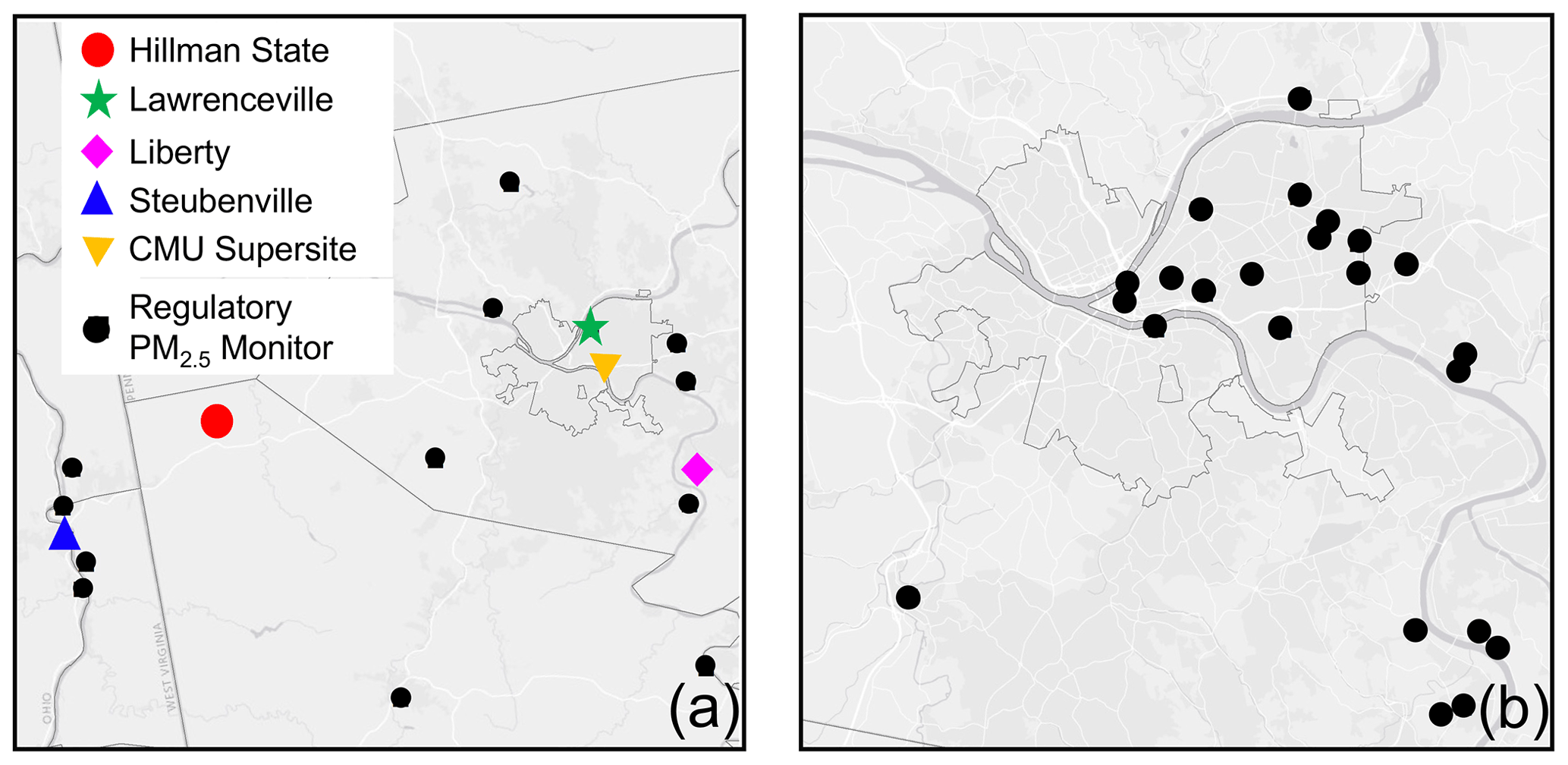
Figure 1 Monitoring sites. (a) Particulate matter speciation measurement sites from EPA-CSN and PM_2.5 regulatory monitors. The entire inner modeling domain is shown. (b) Low-cost sensor sites. City of Pittsburgh boundaries are shown in both panels for reference.

Model predictions of sulfate, nitrate, elemental carbon, and organic aerosol were compared with measurements from 4 sites from the EPA Chemical Speciation Network (EPA-CSN) (U.S. EPA, 2002). The locations of these four sites are shown in Fig. 1a. These sites include Lawrenceville, an urban background site 4 km northeast of downtown Pittsburgh; Hillman State Park, located in a state park in southwest Pennsylvania in a rural and remote location approximately 40 km upwind of Pittsburgh; Steubenville in the Ohio River valley, close to industrial installations and coal-fired power plants; and the Liberty–Clairton monitor, which is located close to the Clairton Coke Works in the Monongahela River valley, 14 km southeast of downtown Pittsburgh. Speciated PM_2.5 measurements from EPA-CSN sites are available every 3 d during the simulation periods. Daily non-speciated measurements of total PM_2.5 mass concentration are available from 17 sites within the inner simulation domain and are used to further evaluate total PM_2.5 mass concentration predictions. The locations of these sites are also shown in Fig. 1a.

For February 2017, high-resolution AMS measurements from the Carnegie Mellon University supersite (Gu et al., 2018) are used to evaluate the predicted chemical composition of PM_2.5 model predictions. Positive matrix factorization results are also used to investigate the breakdown of organic aerosol components. AMS measurements were taken continuously from 1 to 14 February 2017. Due to uncertainties with the AMS collection efficiency during this campaign, here we only use the fractional particle composition data.

PMCAMx predictions of PM_2.5 were also compared with measurements taken with a network of Real-time, Affordable, Multi-Pollutant (RAMP) monitors (Zimmerman et al., 2018) distributed in the city of Pittsburgh. During the winter period, measurements at seven sites were available, all located within the boundaries of the city of Pittsburgh, while 22 sites were in operation during the summer period, with a few sites also outside the city (Fig. 1b). Uncertainty in these low-cost measurements of PM_2.5 mass concentration is between 3–4 µg m⁻³ for hourly averaging times (Malings et al., 2019).

The model performance is assessed in terms of the mean bias (BIAS), the mean error (ERROR), the fractional bias (FBIAS), and the fractional error (FERROR):

$$\begin{array}{}\text{(1)}& {\displaystyle }\text{BIAS=}{\displaystyle \frac{\mathrm{1}}{N}}\sum _{i=\mathrm{1}}^N{P}_i-O_i\text{(2)}& {\displaystyle }\text{FBIAS}={\displaystyle \frac{\mathrm{2}}{N}}\sum _{i=\mathrm{1}}^N{\displaystyle \frac{P_i-O_i}{P_i+O_i}}\text{(3)}& {\displaystyle }\text{ERROR}={\displaystyle \frac{\mathrm{1}}{N}}\sum _{i=\mathrm{1}}^N\left|P_i-O_i\right|\text{(4)}& {\displaystyle }\text{FERROR}={\displaystyle \frac{\mathrm{2}}{N}}\sum _{i=\mathrm{1}}^N{\displaystyle \frac{\left|P_i-O_i\right|}{P_i+O_i}},\end{array}$$

where N is the number of valid measurements, P_i is the predicted concentration, and O_i is the corresponding observed concentration. The fractional error metric is bounded by 0 (perfect prediction performance) and 2.0 (extremely poor prediction performance). Fractional bias is bounded by −2.0 (extreme underprediction) and +2.0 (extreme overprediction).

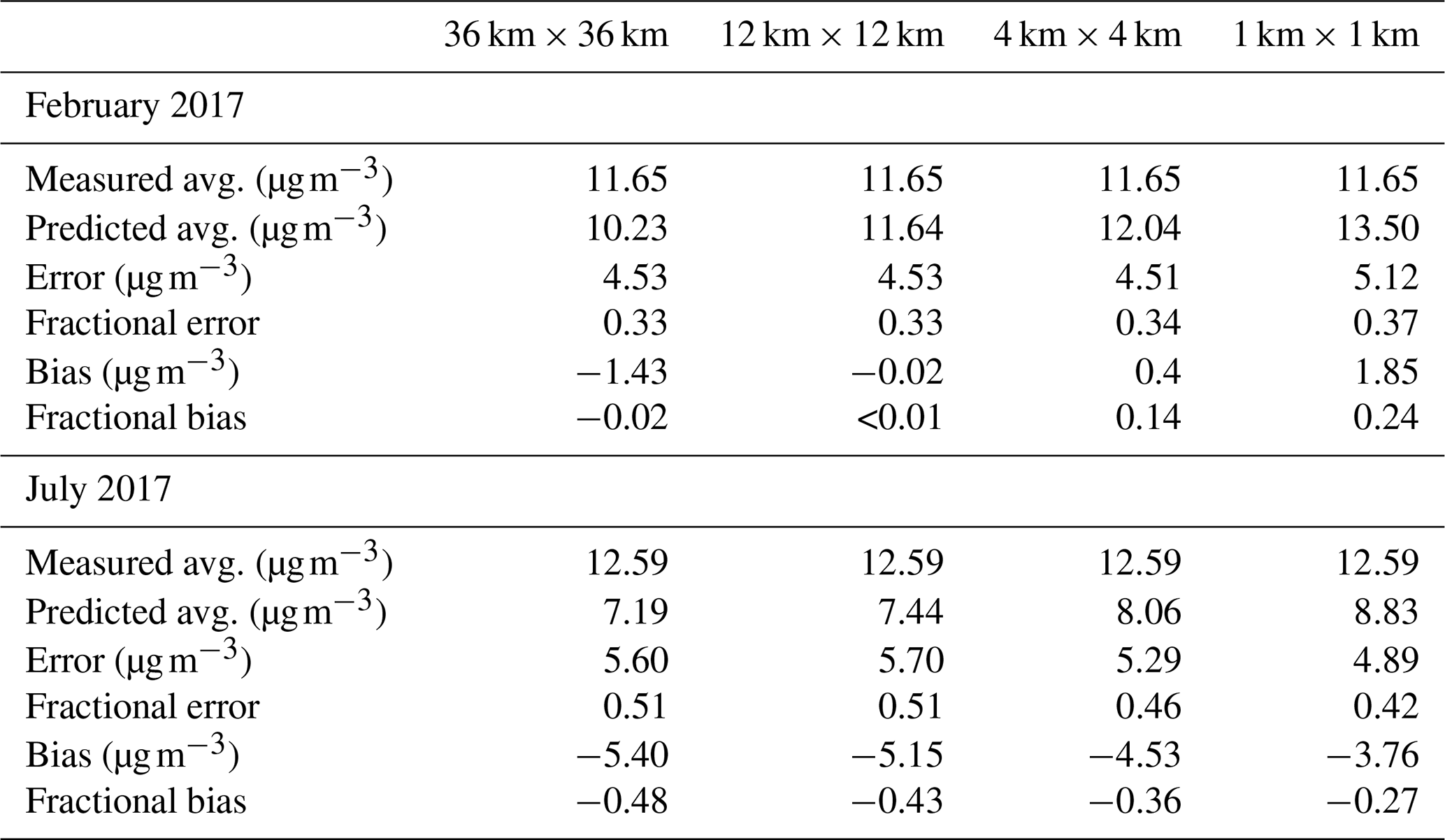
Table 1 Comparison of daily average high-resolution PMCAMx-v2.0 predictions with daily EPA-CSN measurements during February and July 2017.

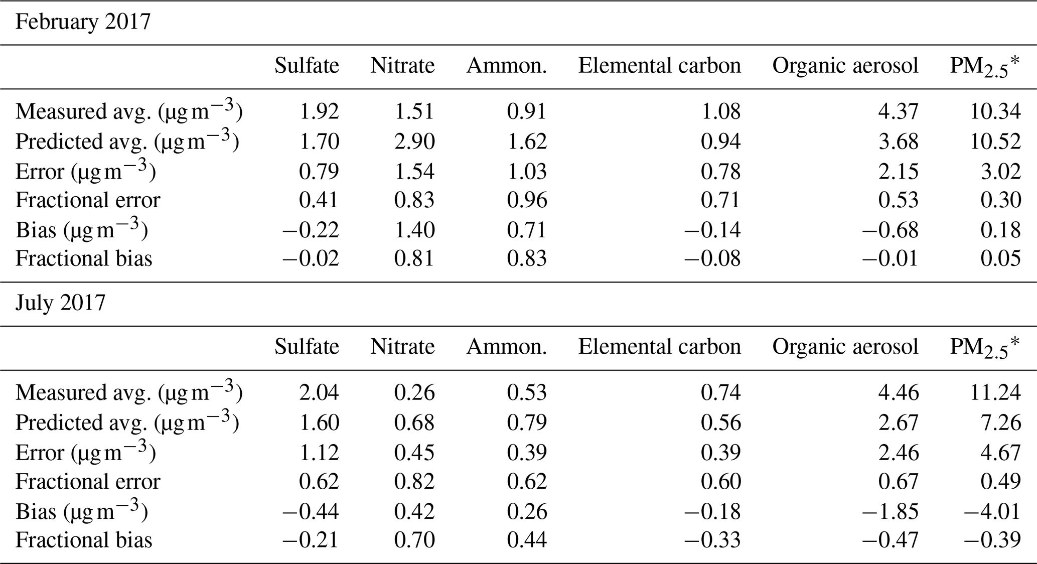
^∗ Measurements from the regulatory EPA monitors.

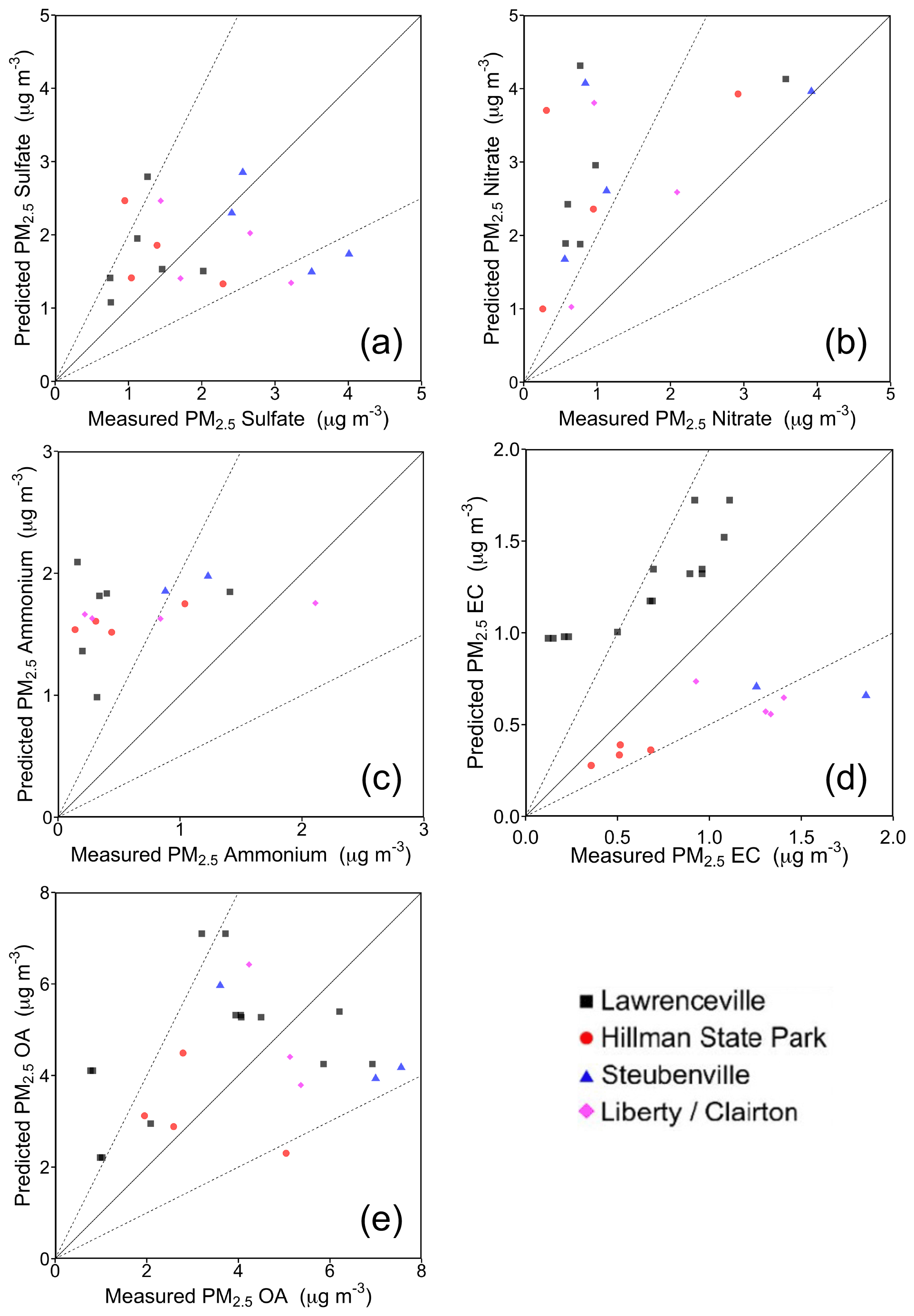
Figure 2 Comparison of daily average PMCAMx-v2.0-predicted concentrations of PM_2.5 (a) sulfate, (b) nitrate, (c) ammonium, (d) elemental carbon, and (e) organic aerosol with daily measurements from EPA-CSN sites during February 2017.

4 Evaluation of high-resolution model performance

4.1 Winter

Table 1 summarizes the performance metrics of daily average PMCAMx-v2.0 PM_2.5 predictions in the 1 km × 1 km resolution, when compared with daily measurements from EPA regulatory PM_2.5 monitors. The speciated performance is illustrated in Fig. 2. Predictions of total PM_2.5 mass perform well against regulatory measurements in the February simulation period, with a fractional error of 0.3 and fractional bias of +0.07.

Average measured PM_2.5 sulfate for this time period was 1.9 µg m⁻³. Lower sulfate levels were observed at the Lawrenceville site in Pittsburgh (1.2 µg m⁻³), while significantly higher levels were observed at the Steubenville site (3.1 µg m⁻³). Predicted domain-average PM_2.5 sulfate at 1 km × 1 km resolution was 1.3 µg m⁻³. Overall fractional error for sulfate predictions was 0.41, and no overall bias was observed (fractional bias of −0.02). PM_2.5 sulfate was slightly overpredicted at Hillman State Park (+0.18 fractional bias) and Lawrenceville (+0.25 fractional bias) and underpredicted at the industrial sites, Steubenville (−0.24 fractional bias), and Liberty/Clairton (−0.43 fractional bias), where observed PM_2.5 sulfate concentrations were higher.

Overpredictions were seen for PM_2.5 nitrate, with a fractional bias of +0.81. The average measured concentration at EPA-CSN sites within the simulation domain was 1.5 µg m⁻³, while the domain-average predicted concentration was 1.8 µg m⁻³. Observed average PM_2.5 nitrate concentrations at Hillman State Park and Lawrenceville were slightly lower at 1.1 µg m⁻³ and 1.2 µg m⁻³, respectively. Nitrate at the Steubenville location was observed to be higher on average at 2.2 µg m⁻³. This overprediction is seen at all sites but is particularly prevalent at Hillman State Park, Lawrenceville, and Liberty/Clairton, where errors are of the order of a factor of 2. Previous PMCAMx modeling studies have found similar overpredictions. Part of this overprediction was due to the use of coarse-grid resolution (Zakoura and Pandis, 2018), but this is unlikely to be the cause here because 81 % of the predicted domain-average nitrate is transported from outside of the inner modeling domain. These inconsistencies in PM_2.5 nitrate predictions are likely due to errors in the partitioning of nitrate between the fine (PM_2.5) and coarse (PM₁₀) modes, resulting in an overprediction of PM_2.5 nitrate. Resolving this modeling error likely requires improvements to the treatment of dust within the model and the use of a dynamic approach for inorganic aerosol calculations rather than the bulk equilibrium approach.

The behavior of PM_2.5 ammonium measurements is similar to that of nitrate as most of it is in the form of ammonium nitrate. The average measured concentration at the four EPA-CSN stations was 0.9 µg m⁻³. At Hillman State Park and Lawrenceville, the measured average was lower at 0.5 µg m⁻³ but higher at the Liberty/Clairton location at 2.1 µg m⁻³. PM_2.5 ammonium was overpredicted similarly to PM_2.5 nitrate, with +0.83 fractional bias.

The average measured concentration of PM_2.5 elemental carbon at EPA-CSN sites during February 2017 was 1.1 µg m⁻³. Elemental carbon concentrations are more localized than the inorganic PM_2.5 components. At Hillman State Park the average measured concentration was only 0.5 µg m⁻³, while at Liberty/Clairton the averaged measured concentration was 2.9 µg m⁻³. For elemental carbon, the predicted domain average was 0.4 µg m⁻³. Average elemental carbon concentration in the 4 km × 4 km simulation grid outside of the inner modeling domain was 0.3 µg m⁻³. Black carbon predictions at all sites had a fractional error of 0.71, with a fractional bias of −0.08. Elemental carbon was overpredicted at the urban site, with a fractional bias of 0.73, and underpredicted at the other sites.

Average measured organic aerosol (OA) during this period was 4.4 µg m⁻³ but with significant spatial variability. At Hillman State Park and Lawrenceville, measured OA was 3.1 µg m⁻³ and 3.4 µg m⁻³, respectively. At Liberty/Clairton and Steubenville, the average measured OA was 7 µg m⁻³ and 6.3 µg m⁻³, respectively. Domain-average predicted OA was 2.2 µg m⁻³. Outside of the inner 1 km × 1 km domain, average predicted OA was 1.6 µg m⁻³, suggesting that the majority of predicted OA is transported from outside of the 1 km × 1 km grid. Overall OA prediction performance in the winter is acceptable at 0.53 fractional error and low fractional bias (−0.01). At individual sites, performance varies. OA is predicted with low fractional bias (−0.10) at the rural Hillman State Park site. OA is overpredicted with +0.31 fractional bias at the urban site in Lawrenceville and underpredicted at both industrial sites. An added degree of uncertainty exists with the industrial sites within the inner domain. The emissions from these sources may be underestimated in the inventory, and these locations are also difficult to accurately model due to their geographic location in river valleys.

Average concentrations of PM_2.5 sulfate, nitrate, and ammonium in the 4 km × 4 km resolution domain were around 83 % of the average predicted concentrations in the inner 1 km × 1 km simulation grid. For elemental carbon and OA, the outer concentration was 64 % and 73 % of the inner concentration, respectively, indicating that these species had significant local sources. For these more local pollutants, the model appears to perform well in terms of capturing urban–rural gradients but with a tendency towards underprediction at the rural site in Hillman State Park and overprediction at the urban site in Lawrenceville. The model also underpredicts elemental carbon (EC) and OA at the industrial locations, especially elemental carbon (−0.67 and −1.02 fractional bias at Steubenville and Liberty/Clairton, respectively). This again suggests errors in the emissions inventory or problems in simulating atmospheric dispersion near the sources.

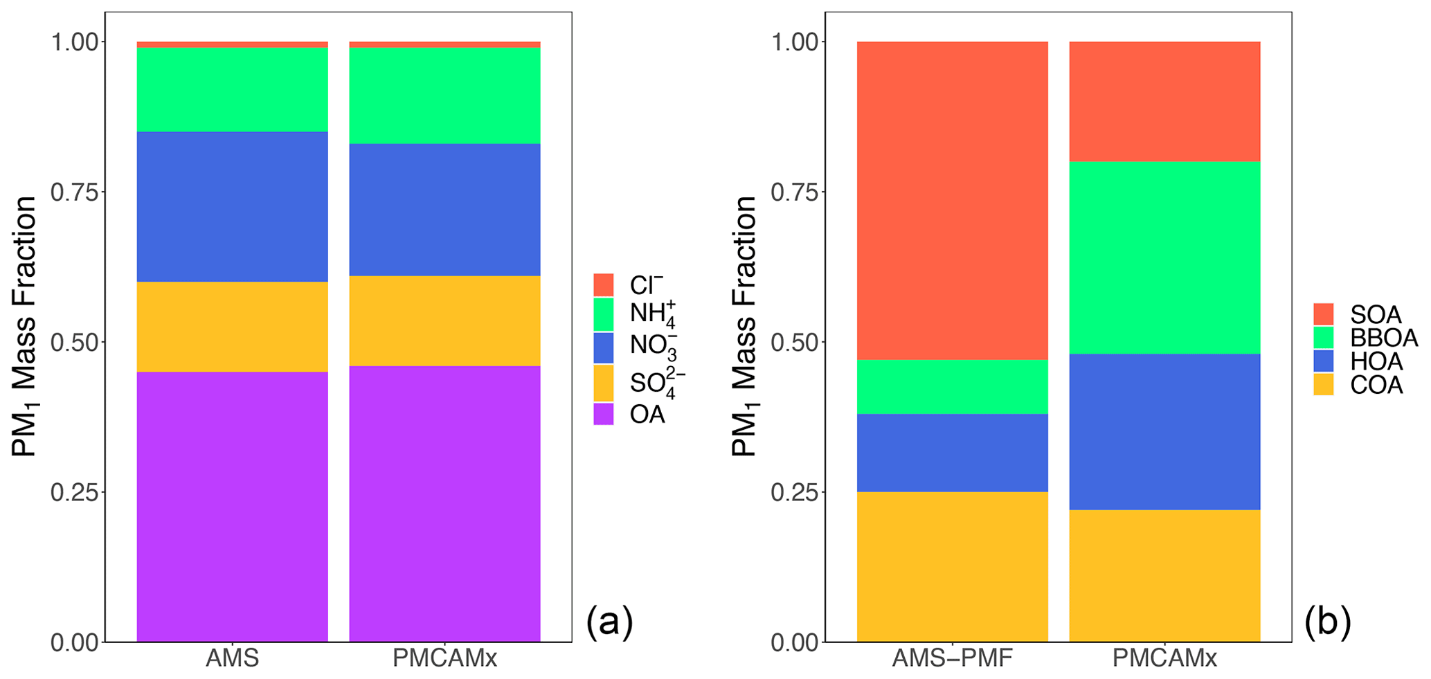
Figure 3 (a) Comparison of PMCAMx-v2.0-predicted composition of PM₁ with the corresponding AMS measurements at the CMU site and (b) organic aerosol composition based on the PMF analysis of the AMS measurements and predicted composition.

Comparisons with the PM₁ composition, as determined by the AMS from 3 through 14 February 2017, show excellent agreement for all species (Fig. 3a). Gu et al. (2018) used positive matrix factorization (PMF) analysis and allocated total measured OA into five factors. Three of them corresponded to primary organic aerosol, hydrocarbon-like OA (HOA), cooking OA (COA), and biomass burning OA (BBOA), and there were two secondary OA factors, more-oxidized organic aerosol (MO-OOA) and less-oxidized organic aerosol (LO-OOA). To compare PMCAMx predictions with the primary PMF factors, two additional simulations were performed in which emissions from biomass burning and commercial cooking were set to zero. The predicted concentrations were then subtracted from the base case to estimate the contribution from each respective source. The remaining primary OA was assigned to HOA. The LO-OOA and MO-OOA factors were added together and compared with the PMCAMx SOA predictions.

The predicted cooking OA (COA) at the CMU site is 25 % of the total OA and is in agreement with the PMF/AMS estimate of 22 % (Fig. 3b). This is encouraging given the small bias of the model for total OA levels. The predicted HOA and BBOA are higher than measured by a factor of 2 or more. At the same time, the measurements indicate a surprisingly high contribution of SOA (53 % of the total OA) during a period with little photochemical activity and low levels of OH radicals. SOA is predicted to be just 20 % of the total during this time period. These discrepancies may indicate transformation of the HOA and BBOA to OOA during this wintertime period that is not included in the model. Kodros et al. (2020) recently suggested that BBOA can react with the NO₃ radical during the winter and can be transformed to OOA.

4.2 Summer

Total PM_2.5 mass concentrations are underpredicted in the summer period. The average measured PM_2.5 value in the regulatory network in the area was 11.4 µg m⁻³, while the average predicted value at the regulatory sites was 4 µg m⁻³ lower.

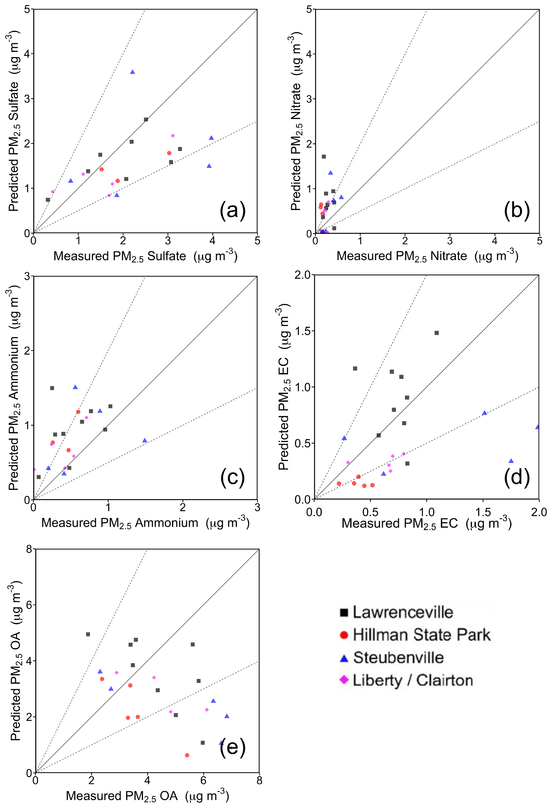
Figure 4 Comparison of PMCAMx-v2.0-predicted concentrations of PM_2.5 (a) sulfate, (b) nitrate, (c) ammonium, (d) elemental carbon, and (e) organic aerosol with measurements from EPA-CSN sites during July 2017.

Speciated PM_2.5 performance is illustrated in Fig. 4. Average measured PM_2.5 sulfate for the summer period was 2 µg m⁻³. Slightly lower levels were observed at the Lawrenceville site in Pittsburgh (1.9 µg m⁻³). Liberty/Clairton had higher measured sulfate concentrations (2.6 µg m⁻³), but this difference between locations is lower than what was observed in the winter period. Predicted domain-average PM_2.5 sulfate at 1 km × 1 km resolution was 1.3 µg m⁻³. Overall fractional error (0.62) and fractional bias (−0.21) for sulfate predictions was higher than in the winter simulation period. PM_2.5 sulfate was underpredicted at all sites but to the largest extent at Hillman State Park (−0.36 fractional error).

Overpredictions of PM_2.5 nitrate were also seen in the summer period and at all types of sites. Average measured PM_2.5 nitrate was 0.3 µg m⁻³, much lower than in the winter. The domain-average predicted PM_2.5 nitrate was 0.7 µg m⁻³. Again, predicted PM_2.5 nitrate in the inner domain is dominated by material transported from outside the boundaries (75 %), so the issue is not resolved by using a high-resolution grid. Improvements to PM_2.5 nitrate formation are needed in the form of dust models with increased complexity to resolve the issues with fine–coarse-mode partitioning of particulate nitrate. These issues have been highlighted by decreased concentrations of PM_2.5 pollution in recent years.

Observed PM_2.5 ammonium concentrations at EPA-CSN sites were also much lower in the summer, with an average value of 0.5 µg m⁻³. Slightly higher average concentrations were observed at Liberty/Clairton (0.7 µg m⁻³), and slightly lower concentrations were observed at Steubenville (0.4 µg m⁻³). The domain-average predicted PM_2.5 ammonium concentration was 0.6 µg m⁻³. The average concentration directly outside of the inner domain was 0.5 µg m⁻³. Overall performance was better for ammonium in the summer than in the winter, with a fractional error of 0.62 and fractional bias of +0.44. The strongest overprediction is seen at the Steubenville site (+0.57 fractional bias).

The average measured elemental carbon (EC) concentration in July was 0.7 µg m⁻³. Measured EC carbon was significantly higher at Liberty/Clairton (1 µg m⁻³) and lower at rural Hillman State Park (0.4 µg m⁻³). Domain-average predicted EC was 0.3 µg m⁻³. Outside of the inner domain, the average predicted concentration was 0.2 µg m⁻³. Elemental carbon predictions in July had a lower fractional error compared to the winter at 0.60 but showed a stronger negative fractional bias at −0.33. The model severely underpredicts at Hillman State Park (−0.86 fractional bias), where measured concentrations were lowest, but also at the industrial sites of Steubenville (−0.55 fractional bias) and Liberty/Clairton (−0.65 fractional bias). EC was slightly overpredicted at the urban Lawrenceville location (+0.14 fractional bias). While the urban–rural gradient in EC is slightly overpredicted, the model is still able to capture the variability between rural (Hillman State Park) and urban (Lawrenceville) sites well. The model struggles to reproduce high measurements of EC at the Steubenville site, reiterating the issues with industrial EC seen in the winter.

Table 2 Comparison of daily average PMCAMx-v2.0-predicted PM_2.5 concentrations during February and July 2017 with daily measurements from 17 EPA regulatory monitors.

Average measured OA concentration was 4.5 µg m⁻³ in July. Higher concentrations were observed at the industrial sites, Liberty/Clairton and Steubenville (5.0 µg m⁻³), respectively. The lowest observed concentration was in Hillman State Park (3.6 µg m⁻³). The average predicted concentration at CSN sites was 2.7 µg m⁻³. On average, OA is underpredicted, with a fractional bias of −0.47. This underprediction occurs at all sites but is less prevalent at the urban Lawrenceville location (−0.19 fractional bias) and is most dramatic in Steubenville (−0.65 fractional bias). Because such a large fraction of the OA in the summer is predicted to be secondary (50 % of local OA on average) and transported from outside of the inner modeling domain (84 % of total OA), treatment of SOA formation is likely a key factor contributing to the underprediction of PM_2.5 in the summer. While these improvements are necessary for overall model improvement, they do not have significant impact on the urban–rural gradients which are the focus of this work and are driven by primary species. The performance of EC predictions in various locations is encouraging with regard to primary PM_2.5 performance.

5 Effect of grid resolution on PM_2.5 performance

To determine the effect of grid resolution on the ability of the model to resolve geographical variations in PM_2.5 concentrations, daily average measurements from the 17 EPA regulatory sites were compared with PMCAMx predictions from simulations at 36, 12, 4, and 1 km. The PMCAMx performance metrics are summarized in Table 2.

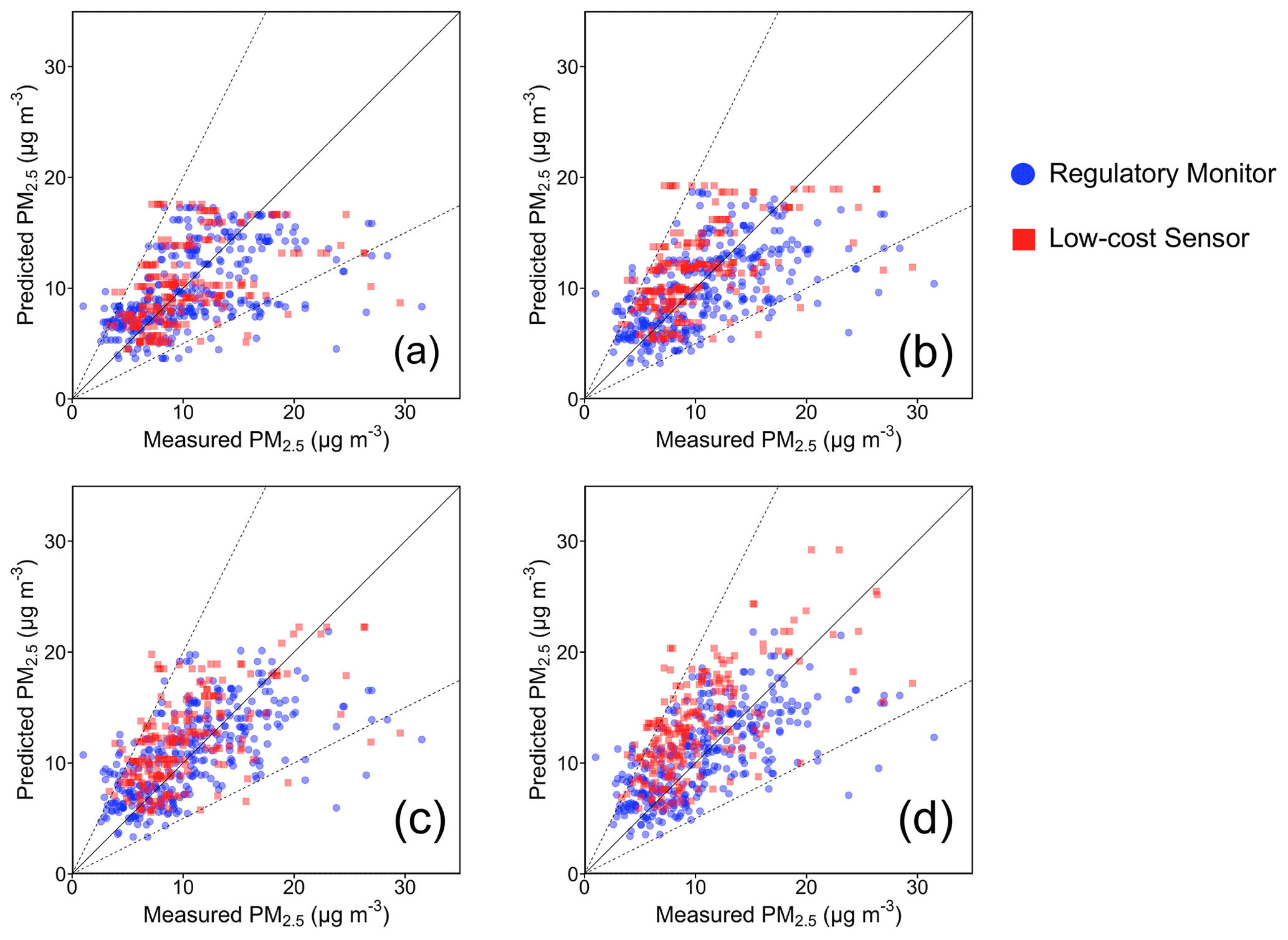
Figure 5 Comparison of daily average PMCAMx-v2.0-predicted concentrations of PM_2.5 with daily regulatory measurements and daily low-cost sensor measurements at (a) 36 × 36, (b) 12 × 12, (c) 4 × 4, and (d) 1 km × 1 km during February 2017.

5.1 Winter

During the winter period, increasing grid resolution reduces the average fractional error from 34 % at 36 km × 36 km to 30 % at 1 km × 1 km. The higher resolution also improved the fractional bias, from −0.09 at 36 km × 36 km to +0.05 at 1 km × 1 km. The performance is illustrated in Fig. 5. Performance at urban locations stayed steady in the winter, with fractional error changing from 0.30 to 0.26 and fractional bias changing from +0.02 to +0.08 moving from 36 to 1 km resolution (Fig. S3 in the Supplement). Rural performance improved to a greater extent, with fractional error improving from 0.33 to 0.28 and fractional bias lowering from +0.21 to +0.11.

Table 3 Comparison of daily average PMCAMx-v2.0-predicted PM_2.5 concentrations during February and July 2017 with daily low-cost sensor (RAMP) measurements.

The comparison with low-cost sensor measurements largely represents the performance of the model in terms of urban PM_2.5 predictions. The performance metrics of PMCAMx-v2.0 when compared to measurements from low-cost sensors are shown in Table 3. Moving from low to high resolution, the predictions go from no bias (−0.02) to a bias of +0.24. Due to the slight overprediction of the urban–rural gradient seen earlier (particularly with EC), the high resolution would likely lead to more positive biases when compared to a largely urban network. Fractional error increases slightly but still exhibits good performance moving from 0.33 to 0.37.

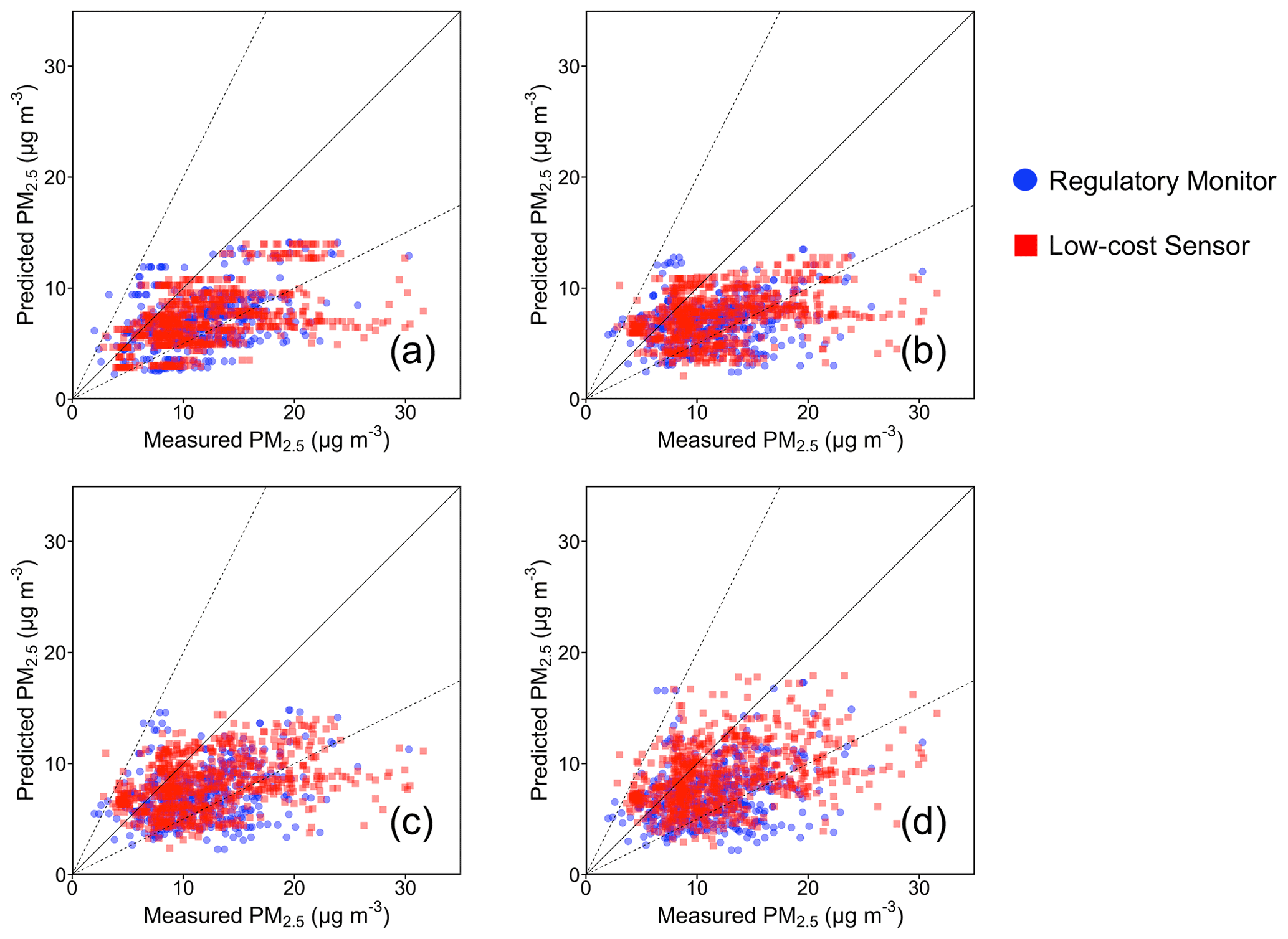
Figure 6 Comparison of daily average PMCAMx-v2.0-predicted concentrations of PM_2.5 with daily regulatory measurements and daily low-cost sensor measurements at (a) 36 × 36, (b) 12 × 12, (c) 4 × 4, and (d) 1 km × 1 km during July 2017.

5.2 Summer

In the summer period (Fig. 6), the model performance improved as the resolution increased from 36 to 1 km. Fractional error decreased from 0.53 to 0.48, while fractional bias increased from −0.46 to −0.39. In July, performance at the urban locations significantly increased with resolution (Fig. S4 in the Supplement). Fractional error decreased from 52 % at 36 km × 36 km to 0.42 at 1 km × 1 km. Fractional bias also improved from −0.46 at the coarse grid resolution to −0.39 at the finest scale. Rural predictions of PM_2.5 were also better, with increasing resolution in the summer. Fractional error decreased from 0.31 to 0.22, while fractional bias decreased from +0.05 to −0.05.

Larger improvements are seen with increasing resolution during the summer when compared to measurements from low-cost sensors. Starting from a large negative bias of −5.4 µg m⁻³ (fractional bias of −0.48) at the 36 km × 36 km resolution, performance consistently improved with each increasing resolution step, with the bias eventually reaching −3.7 µg m⁻³ (fractional bias of −0.27) at the 1 km × 1 km resolution. There was also a reduction in fractional error from 0.52 at the coarse resolution to 0.41 at the fine 1 km × 1 km resolution. These metrics are encouraging, although they are likely impacted by an overprediction of the urban–rural gradient, similar to winter. Improvement of the secondary PM_2.5 predictions is still the largest source of error between predictions and this source of measurements.

6 Evaluation of novel emissions surrogates

For commercial cooking, the normalized restaurant count was used to distribute the emissions from the sector in space within the 1 km × 1 km domain. Geographical information was collected for all restaurant locations in the inner domain from the Google Places application programming interface. This includes southwestern Pennsylvania as well as parts of eastern Ohio and northern West Virginia. To allocate on-road traffic emissions, the output from the traffic model of Ma et al. (2020) was used. This model simulated hourly traffic using data from the Pennsylvania Department of Transportation sites located throughout the inner modeling domain. The use of new surrogates resulted in a new spatial distribution of emissions for both cooking and on-road traffic sources when compared to those developed using default emissions surrogates. The changes in spatial distributions are illustrated in the Supplement (Figs. S5–S8). These novel emissions surrogates resulted in larger emissions of both traffic and cooking in the downtown area. In the case of on-road traffic, major highways in the inner domain are emphasized with the new surrogates.

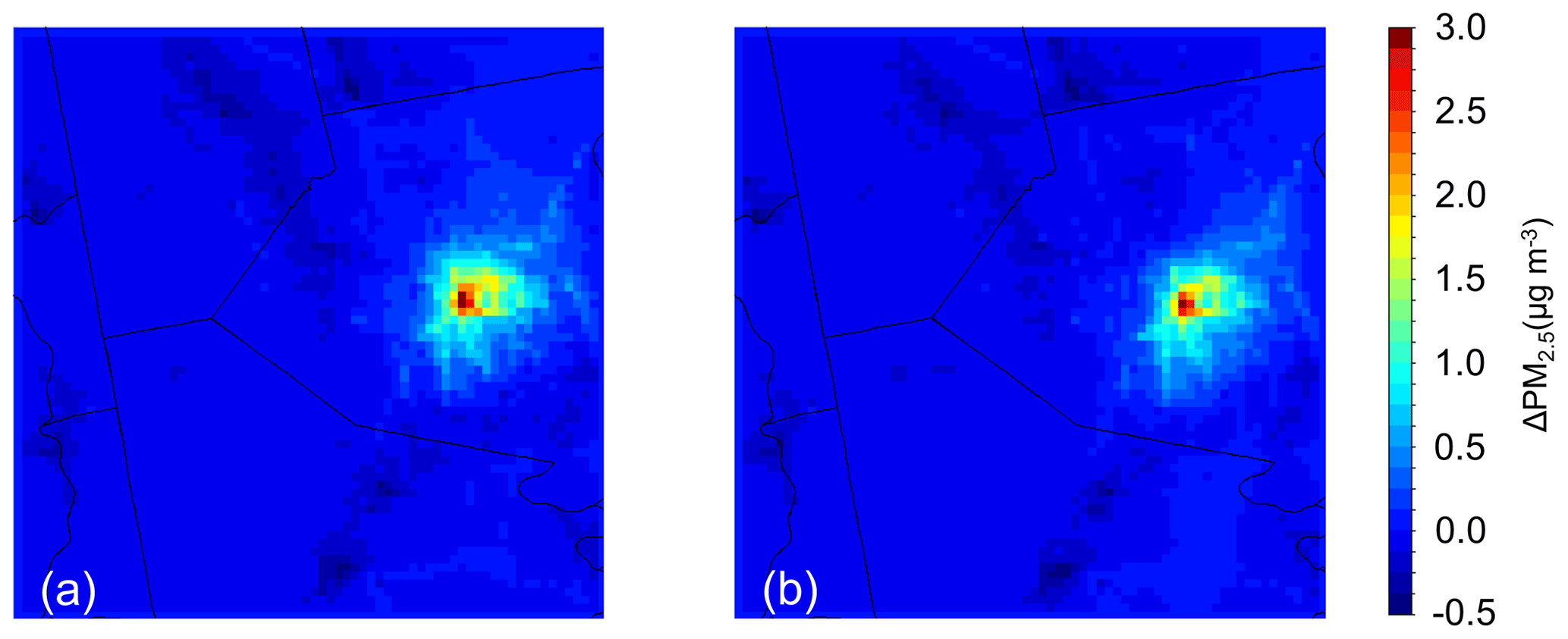
Figure 7 Difference between predicted monthly average PM_2.5 mass concentration when using novel surrogates and original surrogates in (a) February 2017 and (b) July 2017 for the 1 km × 1 km resolution simulation grid. A positive value indicates a higher concentration predicted with the novel surrogates.

For both February and July 2017, the largest observed change when using the novel surrogates is an increase in predicted PM_2.5 of around 3 µg m⁻³ in the downtown Pittsburgh area (Fig. 7). Differences in predicted PM_2.5 concentrations outside of the urban areas of the inner domain are very small (less than 0.5 µg m⁻³ in magnitude).

Table 4 Performance of daily average predicted total PM_2.5 concentrations compared to daily measurements from regulatory sites and low-cost sensors with the use of old surrogates and new surrogates for on-road traffic and commercial cooking within the 1 km × 1 km resolution grid.

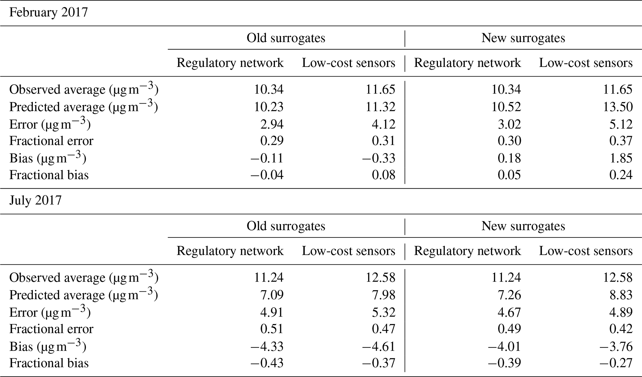
Model performance at 1 km × 1 km resolution is detailed in Table 4. Negligible changes in performance were seen using EPA regulatory PM_2.5 data in February 2017. Small improvements were seen at regulatory sites in July 2017, where fractional error was reduced from 51 % to 48 % and fractional bias increased from −43 % to −39 %. A positive shift in fractional bias was seen with the use of the new surrogates during both periods when compared to low-cost sensor measurements, resulting in a modest overprediction of PM_2.5 in the winter (+0.24 fractional bias) and a modest underprediction of PM_2.5 in the summer (−0.27 fractional bias). The larger changes when compared to the low-cost sensor measurements are a result of the location of the low-cost sensors in urban areas, where the new surrogates predicted elevated PM_2.5 mass concentrations.

7 Conclusions

We applied PMCAMx-v2.0 over southwestern Pennsylvania during February and July 2017 at grid resolutions of 36, 12, 4 and 1 km. Emissions were calculated for the relevant grids using the spatial surrogates provided along with the 2011 NEI for all emissions sectors except traffic and cooking, for which 1 km × 1 km spatial surrogates were developed.

PMCAMx predicts winter sulfate, elemental carbon, and organic aerosol concentrations with fractional biases below 10 % at high resolution. Nitrate concentrations are overpredicted (bias +1.4 µg m⁻³), following the trend of previous studies in both the US and Europe. Agreement with total PM_2.5 measurements is also encouraging, with a fractional bias of +5 %. Variability between urban and rural predictions of local pollutants EC and organic aerosol (OA) is reproduced well in the winter period. Underpredictions of summer OA concentrations led to underpredictions of total PM_2.5 mass. Summer sulfate is reproduced with a fractional bias of −21 %, and elemental carbon (EC) is predicted with a fractional bias of −33 %. Nitrate is similarly overpredicted in the summer, with a fractional bias of +70 %, although with a much smaller magnitude than in the winter (+0.4 µg m⁻³). Differences between urban and rural EC are also predicted well in the summer, while OA is predicted to vary little between urban and rural locations. This is indicative of a greater contribution of secondary species to OA during this period.

PM_2.5 prediction performance improved in almost all cases when increasing the resolution from 36 to 1 km. Underpredictions at urban sites and overpredictions at rural sites were reduced at the same time. This is true when comparing against measurements from regulatory sites as well as low-cost monitors. The improved performance here is evidence of the enhanced ability of the model to capture important urban–rural gradients in PM_2.5 pollution by increasing the resolution of predictions to 1 km × 1 km. Increasing resolution of predictions has been shown here to improve model performance when comparing predicted PM_2.5 concentrations with observations from regulatory monitors and low-cost sensors. However, these simulations highlight the need for specific improvements to some of the secondary PM_2.5 formation pathways in the model. Improvement of the treatment of dust in the model is required to better model the distribution of particulate nitrate between PM_2.5 and PM₁₀ modes. Additionally, improvements to SOA formation chemistry within the model, particularly from biogenic sources outside of the inner modeling domain, will likely have a significant impact on PM_2.5 predictions around the city of Pittsburgh.