the Creative Commons Attribution 4.0 License.
the Creative Commons Attribution 4.0 License.
 | 09 Dec 2022
Inclusion of a cold hardening scheme to represent frost tolerance is essential to model realistic plant hydraulics in the Arctic–boreal zone in CLM5.0-FATES-Hydro
Marius S. A. Lambert
Kjetil S. Aas
Frode Stordal
Rosie A. Fisher
Yilin Fang
Junyan Ding
Frans-Jan W. Parmentier
As temperatures decrease in autumn, vegetation of temperate and boreal ecosystems increases its tolerance to freezing. This process, known as hardening, results in a set of physiological changes at the molecular level that initiate modifications of cell membrane composition and the synthesis of anti-freeze proteins. Together with the freezing of extracellular water, anti-freeze proteins reduce plant water potentials and xylem conductivity. To represent the responses of vegetation to climate change, land surface schemes increasingly employ “hydrodynamic” models that represent the explicit fluxes of water from soil and through plants. The functioning of such schemes under frozen soil conditions, however, is poorly understood. Nonetheless, hydraulic processes are of major importance in the dynamics of these systems, which can suffer from, e.g., winter “frost drought” events.
In this study, we implement a scheme that represents hardening into CLM5.0-FATES-Hydro. FATES-Hydro is a plant hydrodynamics module in FATES, a cohort model of vegetation physiology, growth, and dynamics hosted in CLM5.0. We find that, in frozen systems, it is necessary to introduce reductions in plant water loss associated with hardening to prevent winter desiccation. This work makes it possible to use CLM5.0-FATES-Hydro to model realistic impacts from frost droughts on vegetation growth and photosynthesis, leading to more reliable projections of how northern ecosystems respond to climate change.
- Article
(4487 KB) - Full-text XML
-
Supplement
(1746 KB) - BibTeX
- EndNote


In the Arctic–boreal region, winters are dark, typically last over 6 months, and average temperatures are low (generally around −20 ∘C). To survive the harsh winters of this region, cold-adapted vegetation goes through a set of physiological and structural changes to avoid desiccation and frost mortality (Bansal et al., 2016; Chang et al., 2021). This capacity of plants to withstand freezing can be highly variable throughout the year – depending on the species and environmental factors such as light and temperature. In summer, the tolerance to freezing is low, but it slowly increases when exposed to a decrease in photoperiod and temperature (Beck et al., 2004) – a process known as cold acclimation (Li et al., 2004; Wisniewski et al., 2018). Cold acclimation triggers multiple physiological and biochemical responses which enable plants to (i) tolerate extracellular ice formation and the resulting cellular dehydration (Levitt, 1980; Janská et al., 2010), (ii) avoid the formation of interstitial ice crystals by keeping tissues isolated from the cold and/or by regulating nucleation. Ice nucleation can be suppressed down to −38 ∘C if biological anti-freeze proteins such as dehydrins and flavonoids are synthetized (Hanin et al., 2011) – a process called supercooling. Between −20 and −30 ∘C, the formation of intracellular glass (vitrification) further enables cold-acclimated woody plants to develop a resistance to much lower temperatures. Trees in northern latitudes have evolved resistance to naturally occurring temperatures as low as −70 ∘C (Sakai, 1983), whereas herbaceous plants can rarely tolerate < −25 ∘C. Experiments have demonstrated that trees can resist the temperature of liquid nitrogen (−196 ∘C) when regulating ice nucleation (Rinne et al., 1998).
Plants exposed to temperatures below their tolerance threshold (which varies as a function of time and environmental conditions) suffer from (1) mechanical stress due to the intercellular ice crystallization and fragility of the tissues and (2) osmotic dehydration due to the freezing of intercellular water. Therefore, the increased survival of plant cells and tissues is the evolutionary benefit of cold acclimation. The two strategies of tolerance and avoidance are often found simultaneously in the same plant. Cold acclimation strategies, rates, and ranges involve complex species-dependent physiological and gene expression changes (Chinnusamy et al., 2006; Welling and Palva, 2006).
The physiological adaptations induced by cold acclimation have a large impact on the hydraulics of plants. Apoplastic ice formation and the increased viscosity of protein-bound water particles are known to reduce water flow (Dowgert and Steponkus, 1984; Gusta et al., 2005; Smit-Spinks et al., 1984). In addition, water stress resulting from deeply frozen soils with low soil water potentials triggers slow developmental changes in the root structure to increase their impermeability and reduce water loss (Beck et al., 2007; Kreszies et al., 2019; North and Nobel, 1995). Other strategies include the creation of an air gap during root shrinkage (Carminati et al., 2009; North and Nobel, 1997) and the inhibition of conducting channels (Knipfer et al., 2011; Lee et al., 2005; Ye and Steudle, 2006). Since water transport is prohibited in cold-acclimatized tissues, growth is also affected and it is important that plants de-acclimate rapidly in spring to reactivate their metabolism.
Plant hydraulics, apart from their critical role in the survival of plants during droughts, are also a major driver of species distribution (Fontes, 2019; Lopez-Iglesias et al., 2014; Navarro et al., 2019; Rasztovits et al., 2014). Species distribution is shaped by mortality and recruitment, and the ability of species to survive under periods of low water availability depends on their hydraulic traits (Greenwood et al., 2017). Tolerance to and delay of desiccation, for example, involve traits such as greater resistance to embolism (i.e., interruption of water flow through plant conductive vessels), the ability of cells to remain alive at low water levels, and the reduction of water loss (Kursar et al., 2009; Tyree et al., 2003).
Despite their importance, terrestrial biosphere models typically rely on simple approaches to represent plant hydraulics, involving an extension of Darcy's law. Darcy stated that the flux of water anywhere in the soil–plant continuum was proportional to the hydraulic conductivity and the water potential gradient (Darcy, 1856). One of the simplest implementations of this is to model soil–root conductance as a function of soil moisture (Jarvis and Morison, 1981; Bonan et al., 2014). In more complex models, variable xylem conductance and water potential are added (Williams et al., 2001; Duursma and Medlyn, 2012). One of the most advanced approaches is the continuous porous media approach (Edwards et al., 1986; Sperry et al., 1998; Christoffersen et al., 2016; Mirfenderesgi et al., 2016), which extends the water mass balance in the soil–plant–atmosphere continuum by relating changes in water content directly to water potential and vice versa. Analogous to retention curves in soil physics, the model uses the explicit relationship between water content and potential in plant xylem (pressure–volume curves). The use of plant traits to parameterize such models, as well as their ability to predict measurable features of plant water relations (leaf water potential, sap flow), makes these models attractive from the perspective of both realism and connection to data. Furthermore, such models enable bidirectional water flow through root tissue. Reverse flow from roots to soil is an important process for hydraulic redistribution and tissue dehydration in the case of extreme drought (Oliveira et al., 2005; Nadezhdina et al., 2010; Prieto et al., 2012). A hydraulic model incorporating these advanced mechanisms has recently been included in the Functionally Assembled Terrestrial Ecosystem Simulator (FATES).
FATES is a size- and age-structured representation of vegetation dynamics, which can be coupled to a land surface model or an Earth system model (Christoffersen et al., 2016). CLM (Lawrence et al., 2019) and the Energy Exascale Earth System Model (E3SM) have both been coupled to FATES, and it is used by numerous scientists across the globe to simulate land surface processes (Koven, 2019).
The new plant hydraulics scheme in FATES was initially developed for specific sites in the tropics, and to our knowledge, porous media hydraulics models have not been applied extensively, if at all, in high-latitude or cold systems. Thus, the physiology of plant hydraulics in winter is generally not well represented in such schemes. In the default scheme, for example, stored plant water remains liquid even when temperatures drop below zero and plant gas exchange can continue in the event of frozen soils. In the cold regions of the world, extreme winters can cause soils to freeze to temperatures well below −20 ∘C. Such cases lead to extremely low water potentials in the soil compared to the plant, while the model assumes that water remains liquid inside the plant. Due to this difference in water potential, soils tend to pull water from vegetation, depleting plant storage pools and incurring large amounts of hydraulic failure mortality in the model.
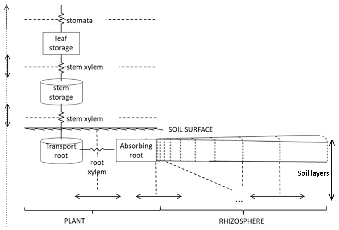
Figure 1Structure of the FATES-Hydro model (Xu et al., 2020).
In this study, we investigate how a model can represent the processes that lead to cold acclimation by implementing a hardening scheme into the CLM5-FATES-Hydro demographic land surface model. The scheme that represents hardening is configured such that cold-acclimated plants reduce conductances along the soil–plant–atmosphere continuum and the rate for hydraulic failure mortality. We explore additional configurations of the scheme wherein hardening of plants led to changing pressure–volume curves and a reduction of the carbon starvation mortality. The modification of these parameters is intended to mimic the physiological changes plants go through when acclimating to cold and the reduction in their metabolic and water transport capacities. Finally, we assess the sensitivity of the model to the parameters of the hardening scheme (maximum hardiness level and timing of dehardening). We hypothesize that the changes prescribed by the hardening scheme (a) are necessary to model realistic vegetation growth in cold climates and (b) make it possible to use CLM5-FATES-Hydro to model realistic impacts from frost droughts on vegetation growth and photosynthesis, leading to more reliable projections of how northern ecosystems respond to climate change.
2.1 The model
CLM5.0-FATES-Hydro stands for the fifth version of the Community Land Model, coupled to the Functionally Assembled Ecosystem Simulator (FATES) with the modified trait-based hydraulic scheme (Hydro-TFS). In this context, CLM5.0 represents the biogeophysical aspects of the land surface, including the energy balance, soil hydrology, biophysics, and cryospheric processes, as well as soil biogeochemistry and other land surface types (lakes, urban, glaciers, crops) (Lawrence et al., 2019).
2.1.1 FATES
FATES (Fisher et al., 2015; Koven, 2019) is a cohort-based vegetation demographic model. It has been integrated into CLM5.0 to represent vegetation processes and dynamics while tracking the vertical (in terms of plant height), spatial (in terms of successional age) and biological (in terms of plant functional type) heterogeneity of terrestrial ecosystems. When coupled to the CLM5.0 FATES handles all processes related to live vegetation (including photosynthesis, stomatal conductance, respiration, growth, and plant recruitment and mortality) as well as fire and litter dynamics.
2.1.2 Hydro
The “Hydro” configuration of FATES is a plant hydrodynamic model. Originally developed by Christoffersen et al. (2016), it follows a continuous porous media approach based on the soil–plant–atmosphere continuum described by Sperry et al. (1998). A single mass balance equation describes the coupled soil–plant system, and the relationship between plant water storage and plant water potential is explicitly described. It consists of a discretization of the soil–plant continuum in a series of water storage compartments with variable heights, volumes, water retention, and conducting properties (Fig. 1).
Trees are divided into four types of porous media (leaf, stem, transporting roots, and absorbing roots). Each aboveground plant medium and transporting root consists of a single storage pool, while absorbing roots are divided into vertical compartments by soil layer. The water pools are connected by pathways with defined lengths and conductances. The soil is divided in cylindrical “shells” around the absorbing roots (the rhizosphere), and hydraulic properties are constant across compartments within a given soil type.
The hydraulics in this scheme are governed by the relationships between content, potential, and conductivity of plant tissues. The model requires parameterization of (1) tissue water content vs. potential (the pressure–volume or PV curve), (2) water potential vs. conductivity of plant tissues, and (3) leaf water potential vs. stomatal conductance stress factor. The first two relationships concern every pool within the plant–soil continuum and follow specific equations for plant and soil porous media types. For the soil, we used the formulation of Clapp–Hornberger and Campbell to describe the first two relationships (Campbell, 1974; Clapp and Hornberger, 1978). For the plant, the first relationship (PV curve) is described by two terms: (a) the solute potential (< 0 due to the presence of solutes) and (b) the pressure potential (≥ 0 due to cell wall turgor) (Ding et al., 2014; Tyree and Hammel, 1972). The cell wall turgor pressure is the hydrostatic force that pushes the membrane against the cell wall in excess of ambient atmospheric pressure (Fricke, 2017). The equations to calculate the solute and pressure potentials depend on parameters such as the osmotic potential at full turgor (pinot) and the elastic bulk modulus (epsil). The second relationship (linking plant water potential and conductivity) is calculated using the inverse polynomial of Manzoni et al. (2013) for the xylem vulnerability curve. The fractional loss of total conductance retrieved from this equation is defined at each compartment boundary (Fig. 1) and used to calculate the maximum conductance, KMAX. This parameter depends on plant architectural properties and maximum xylem-specific conductivity, and it relates to the maximum attainable flow of water through the xylem. The fraction of maximum stomatal conductance is used to downregulate the non-water-stressed stomatal conductance (calculated using Ball–Berry, 1987, formulations).
All parameters involved in these relationships are biologically interpretable and measurable plant hydraulic traits. The numerical solution operates every half-hour (time step) and updates water contents and potentials throughout the plant soil continuum.
2.1.3 The 2D solver
A crucial component of the porous media hydrodynamics model is the solver used at each time step to find a solution for cohort-level water fluxes. The first solver implemented in FATES was a tridiagonal and one-dimensional (series of compartments) matrix solver solving the water transport in the plant and rhizosphere soil a layer at a time. Since the solver was not capable of quickly finding a solution during extreme winter conditions, a more efficient two-dimensional (2D) solver using Newton iterations has been implemented as a replacement. In this solution, the water potentials in plant and rhizosphere soils are solved together as prognostic variables. Although the new solver improves the quality of the solution and reduces errors, we ran into numerous solver errors when running simulations in Siberia. In very cold soils, extremely low water potentials (−40 000 MPa) lead to extremely high matric water gradients and prevent successful solution of the flow equations (despite increases in the time resolution and number of iterations). In the frozen soil scheme of CLM5, liquid water becomes absent when soils freeze, leading to infinitely small water potentials. Our solution to this problem was twofold.
-
The calculation of supercooling in soils is limited to −10 ∘C since soil temperature can decrease to −40 ∘C in the uppermost soil layers at extremely cold locations, i.e., eastern Siberia. This solution yields higher water potential values at all times.
-
We imposed a minimum value on the calculation of soil matric potential from liquid water content of −25 Mpa, and a linear interpolation was used from −25 to −35 Mpa. This implementation allows the solver to efficiently find a solution.
Large rates of water percolation and drainage from upper to deeper soil layers has been reported in earlier modeling simulations in Siberia (Sato et al., 2010). Our focus is on the physiology of hardening and not on the supply and demand dynamics of soil moisture; hence, we prescribed a depth to bedrock of 1 m in all simulations.
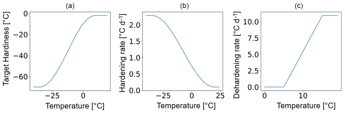
Figure 2Example of (a) the target hardiness (TH), (b) the hardening rate (HR, in ), and (c) the dehardening rate (DR) functions (in ) in relation to the ambient mean temperature corresponding to a site and a plant functional type with a maximum hardiness level (HMAX) of −70 ∘C.
2.2 The hardening scheme
The temporal dynamics of plant hardiness implemented in this study are based on the work by Rammig et al. (2010). In their model, the hardiness level (HD, in ∘C) is calculated on a daily basis using three functions: the target hardiness (TH, in ∘C), the hardening rate (HR, in ), and the dehardening rate (DR, in ) (Fig. 2). In this context, HD is variable throughout the year and represents the minimum temperature plants can withstand without incurring injury.
Once a value has been assigned to TH, HR, and DR, depending on the daily mean 2 m air temperature, the model operates as follows: if TH is lower than the HD of the previous day (HDP), then HR is removed from HDP. By contrast, if TH is higher than HDP, DR is added to HDP (Eq. 1). To illustrate Eq. (1) and the interrelation between HDP and HD, Fig. S14 in the Supplement shows the temporal evolution of TH and HD during 2 random years.
The parameters required for the hardening scheme by Rammig et al. (2010) are the minimum hardiness level (HMIN) of −2 ∘C, the maximum hardiness level (HMAX) of −30 ∘C, HR of 0.1–1 , DR of 0–5 , and several time-dependent parameters used to define the seasons for hardening and dehardening. This scheme was developed to fit the climate of central Sweden (Farstanäs) and measurements of Norway spruce (Picea Abies). Parameters for the hardening scheme (Table S1 in the Supplement) were retrieved from Kellomaki et al. (1995), Jönsson et al. (2004), and Bigras and Colombo (2013).
Due to the large climatic differences between Sweden and eastern Siberia, it is unlikely that the original scheme from Rammig et al. will perform well at Spasskaya Pad. To deal with this, in our adaptation of the hardening model, HMAX becomes site- and time-dependent (to function globally and account for evolution associated with changes in climate) and varies with the 5-year running mean of the annual minimum of daily mean air temperature at 2 m height (T5). An exception is made during the first 5 simulation years. During the first year, HMAX is based on the minimum temperature of the current year, while from the second to fifth years, it is based on the mean of the minimum temperature of the preceding years. HMAX can be anywhere between HMIN (−2 ∘C) and a maximum of −70 ∘C (typical in the Arctic and eastern Siberia) (Sakai, 1983). The functions used to calculate TH (Eq. 2), HR (Eq. 3), and DR (Eq. 4) were made dependent on HMAX so that vegetation can harden and deharden faster at colder sites where HMAX is lower (Fig. 2 shows the functions for HMAX = −70 ∘C).
-
Target hardiness (TH)
-
Hardening rate (HR)
-
Dehardening rate (DR)
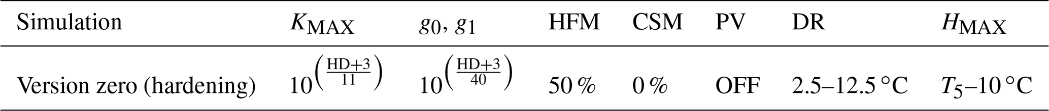
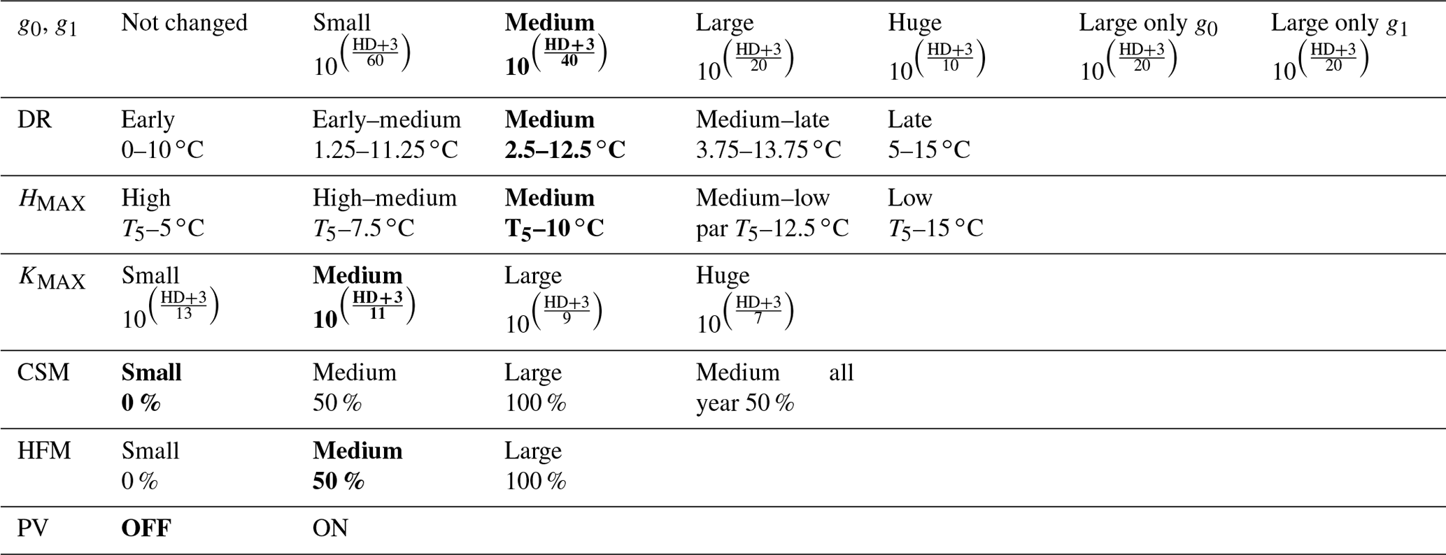
Table 1Configuration of the version zero simulation. This simulation was run at the sites of Spasskaya Pad and Farstanäs for evergreen needleleaf and deciduous broadleaf trees. T5 is the 5-year running mean of the minimum 2 m daily temperature of each year.
In Rammig et al. (2010), the hardening period is prevented until the 210th Julian day and a growing degree day threshold is reached. We instead use a site-specific day-length threshold (DaylThresh) depending on the temperature index T5 of the corresponding site (Eqs. 5 and 6). A site-dependent value for DaylThresh is essential since vegetation at colder sites must start to harden earlier, and the correlation between photoperiod and temperature is not the same at all locations. Finally, to avoid dehardening in autumn, we keep HD fixed during the hardening-only period of the year in cases in which TH is not below HDP (Eq. 6). In our version of the hardening scheme, if the requirements of Eq. (6) are met, the value given to HD in Eq. (1) will be overwritten.
At the end of the time step, values of HD outside the range between HMIN and HMAX will be redefined within these extremes according to Eq. (7).
2.3 Physiological impacts of hardening state on plants
Rammig et al. (2010) used the prognostic hardening state to directly modulate the degree to which frost damages plants. In this study, to enhance the mechanistic basis of the simulations, we used the “hardening” state to simulate the impact of hardening on the hydraulic functioning of the plant in terms of both the benefits of hardening (i.e., prevention of desiccation) and the physiological costs (reduced ability to conduct water and photosynthesize during the hardening and dehardening phases). We did this by modifying KMAX, g0, and g1 as well as the hydraulic failure mortality scalar (see the “version zero” simulation in Table 1). We then explore additional configurations of the scheme wherein hardening of plants led to changing PV curves and a reduction of the carbon starvation mortality.
2.3.1 Maximum conductance between plant compartments (KMAX)
In FATES-Hydro, KMAX is calculated on the upstream (towards the soil) and downstream (towards the atmosphere) sides of each water compartment connection along the soil–plant continuum. The water potential of the system impacts the direction of the flow and thereby the applicable root radial conductance.
During hardening and water stress, apoplastic ice formation, increased viscosity of protein-bound plant water particles, the increased impermeability of root structures, and the inhibition of conducting channels reduce water flow (Dowgert and Steponkus, 1984; Gusta et al., 2005; Smit-Spinks et al., 1984). Therefore, when the hardening scheme is turned on and the hardening level of plants (HD) is lower than −3 ∘C (−2 plus −1 ∘C as a margin), the level of hardening is used to exponentially reduce each of the calculated KMAX values along the soil–plant continuum. In “version zero” (Table 1), KMAX was reduced by (Eq. 7).
2.3.2 Stomatal conductance (g0 and g1)
The calculation of stomatal conductance in this version of FATES-Hydro is based on the Ball–Berry stomatal conductance model. This scheme is typically applied globally, and its parameters and function are not responsive to plant hardening status by default. This means that in winter, when soils are frozen, water loss can still deplete tissue water contents. To prevent desiccation in our scheme, we modify the parameters of the stomatal conductance model as a function of hardening status. The stomatal model has two parameters, the “minimum” conductance, g0, which is the stomatal conductance when photosynthesis reaches zero. In the default setup, g0 is fixed at 10 000 for both evergreen needleleaf and deciduous broadleaf trees. The second parameter, g1, is the slope of the Ball–Berry stomatal conductance model and is fixed at 8 for all C3 plant functional types (PFTs) in the default setup. In our simulations, if HD is lower than −3 ∘C, HD reduces g0 and g1 in a similar way as the reduction of KMAX (Eqs. 8 and 9). In the version zero simulation we reduced g0 and g1 by (Eqs. 8 and 9) (Table 1).

Figure 3Pressure–volume curves for soil (orange) and plant compartments. The PV curves used by the default CLM5-FATES-Hydro and non-hardened plants are the dashed lines, while the PV curves used by plants acclimated to −70 ∘C are the full lines.
2.3.3 Hydraulic failure mortality (HFM)
In the default version of FATES-Hydro, HFM (the hydraulic failure mortality) is triggered when the fractional loss of conductivity (flc) is larger than a predetermined threshold (flcThreshold, set at 0.5). The fractional loss of conductivity is multiplied by a scalar (MortScalar, 0.6 in default FATES) that converts the proximal cause of mortality (conductance loss) into a cohort-specific rate of mortality (fraction/year) (Eq. 10). As shown in the Results section, the default parametrization of HFM used at these cold climate sites leads to systematic, large, and uninterrupted mortality rates throughout the winter on account of desiccation. Since cold-acclimated plants are typically dormant (Chang et al., 2021), and dormant plants are known to have a slower or interrupted metabolism, we tested a scenario in which we reduced HFM with HRATE. HRATE is a version of HD normalized to the value of HMAX (Eq. 11). HRATE was preferred to HD in the reduction of HFM so that if HD is equal to HMAX, the reduction of HFM is at a maximum. In the control hardening simulation we reduced HFM by up to 50 % at HD equal HMAX Eq. (13). In the two sensitivity experiments conducted on HFM, we modified the occurrences of 50 % in Eq. (13) to obtain a reduction reaching 100 % and 0 %, respectively (Table 1).
2.3.4 Pressure–volume curve
PV curves describe the relationship between total water potential and relative water content in the soil and the plant compartments. The formulation of the plant compartment PV curves in FATES-Hydro relies on a set of parameters: osmotic water potential at full turgor and/or saturation (pinot), bulk elastic modulus (epsil), saturation volumetric water content, residual volumetric water content, capillary region parameters, and relative water content at full turgor (see the description of FATES-Hydro in the “Model description” subsection of the Methods section). Among these parameters, the literature has shown that pinot and epsil are highly variable, depending on water deficiency. Stressors that induce water deficiency (e.g., drought, cold, and frost) trigger similar responses at the cellular and molecular level. To maintain turgor during stress (Beck et al., 2007) or during hardening (Valentini et al., 1990), plant organs increase their solute concentration, which decreases pinot, and they increase the elasticity of their cell walls, which corresponds to a decrease in epsil (Bartlett et al., 2012; Kuprian et al., 2018). While research on desert shrubs has shown that epsil increased by roughly 10 Mpa during winter (Scholz et al., 2012), the literature reveals that pinot easily decreases by 0.5 MPa with hardening and during drought stress (Mart et al., 2016; Valentini et al., 1990).
In this section we describe how we made the PV curves for plant mediums vary throughout the year depending on HD (Fig. 3). We lowered the PV curves while daily-updating the osmotic potential at full turgor and the elastic bulk modulus (Eqs. 13 and 14). At an HD of −70 ∘C, we lower the default pinot values for leaves (−1.465984), stems (−1.22807), transporting roots (−1.22807), and absorbing roots (−1.043478) by 0.5 Mpa. The default epsil values (leaves: 12, stems: 10, absorbing roots: 10, transporting roots: 8) are increased by 10 MPa at an HD of −70 ∘C. Unless HD gets below −3 ∘C, the default Hydro PV curve is used, while at its lowest (−70 ∘C), the PV curves are maximally modified. The changes to pinot and epsil modify the shape of the PV curve so that a given water content is linked to a lower water potential.
2.3.5 Carbon starvation mortality (CSM)
Similarly to HFM, CSM (the carbon starvation mortality) is triggered when the carbon stored in the leaves is below a target level, and the fraction of carbon is multiplied by a fixed scalar (set at 0.6 for all plant functional types). CSM is incurred each winter, creating an annual cycle for living biomass of evergreen trees in temperate and boreal regions. In the version zero simulation, CSM is not reduced (Table 1). In the sensitivity experiments, CSM was reduced following the same method as for HFM (Eq. 12).
2.4 Experimental setup
Simulations were carried out using CLM5.0-FATES-Hydro, with fully prognostic state variables for vegetation, litter, and soil. The atmospheric forcing to drive the model simulations was derived from ERA5-Land data (ERA5L) (ERA5-Land monthly averaged from 1981 to present, Muñoz Sabater, 2019). ERA5L provides hourly global high-resolution (9 km) information on surface variables from January 1981 to present day, which makes it a valuable dataset for our hardening scheme analysis. In this study, we retrieved temperature at reference height, wind, humidity, surface pressure, precipitation, downward shortwave radiation, and downward longwave radiation for the entire period. Each simulation was run for 90 years in which the atmospheric forcing from the 30-year period between 1981 and 2011 was repeated three times. These three periods are depicted as the years 1921 to 2011 for convenience.
2.4.1 Site descriptions
We conducted site-specific simulations for Farstanäs (in Sweden) and near Spasskaya Pad (in Russia). These locations were selected to verify and illustrate the behavior of the hardening scheme in distinctly different climates.
Spasskaya Pad is a scientific research station in the taiga near Yakutsk, Russia (62∘ N, 129∘ E), the coldest large city in the world, with an annual average temperature of roughly −9 ∘C. Spasskaya Pad has never recorded a temperature above freezing between 10 November and 14 March, and the average winter temperature is below −20 ∘C. However, the warm summers (with a July average and highest daily mean temperatures of ∼ 20 and ∼ 25 ∘C, respectively) place Spasskaya Pad far south from the tree line. The total yearly precipitation is around 280 mm, and the snow depth typically reaches 40 cm. Spasskaya Pad is in the center of Yakutia, the largest republic of the Russian Federation, which is mostly covered by boreal vegetation (74 %) (Isaev et al., 2010). The forests are mainly composed of Larch (deciduous needleleaf), patches of Scots pine (evergreen needleleaf) on sandy soil (Sugimoto et al., 2002), dwarf Siberian pine (Pinus pumila) and to a lesser extent Siberian spruce (Picea omorika), and small stands of birch (Betula), fir (Abies), and aspen (Populus).
Farstanäs (59∘ N, 17∘ E) is slightly south of Stockholm and presents a cold temperate climate. The mean yearly temperature is around 5.5 ∘C, and the total yearly precipitation is around 800 mm. The vegetation at Farstanäs is a mixed forest with, among others, spruce, pine, beech, oak, elm, ash, and maple.
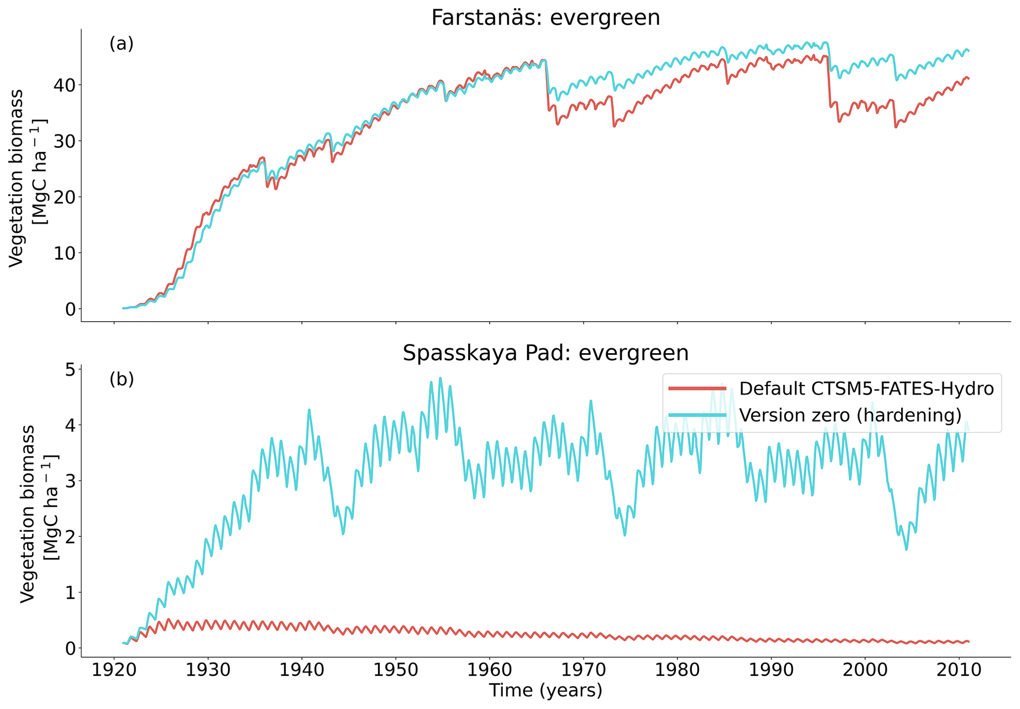
Figure 4Living biomass for needleleaf evergreen trees at the sites of (a) Farstanäs and (b) Spasskaya Pad during the period 1921–2011 (atmospheric forcing: 3 × [1981–2011]). The default simulation is shown in red, and the hardening simulation is shown in blue.
2.4.2 Plant functional type
To remove species competition and better understand the impacts of hardening on vegetation growth, we performed each simulation with only one plant functional type. We tested the scheme on two plant functional types: extratropical evergreen needleleaf trees and cold–deciduous broadleaf trees. Although evergreen needleleaf trees are not the dominant plant type at Spasskaya Pad (Petrov et al., 2011; Tatarinova et al., 2017; Hamada et al., 2004), we selected this location since it is one of the most extreme (cold and dry) climates wherein pine trees still exist. Therefore, we expect that the benefit from introducing a cold hardening scheme may be particularly apparent at this location. Results from broadleaf deciduous simulations are included in the Supplement (Fig. S3). Note that soil conditions, including matric potential, are similar in deciduous and evergreen simulations (Fig. 4).
Table 2Sensitivity experiments run from the version zero hardening simulation (cells and data highlighted in bold). The simulations were run at the sites of Spasskaya Pad and Farstanäs for evergreen needleleaf trees. HD is the hardiness level and T5 is the 5-year running mean of the minimum 2 m daily temperature of each year.
2.4.3 Main simulations
In the first part of our results we compare the implementation of the new hardening scheme (version zero) into CLM5-FATES-Hydro to the default version of the model. In the version zero of the hardening scheme, cold-acclimated plants reduce (I) the maximum conductance between plant tissues and between roots and soil (KMAX), (II) both the intercept and the slope of the stomatal conductance model, and (III) the rate for hydraulic failure mortality (HFM) (Table 1). For the version zero simulation, the values for the reductions of KMAX, g0 and g1, DR, and HMAX were selected based on preliminary testing to minimize winter water losses and to maximize vegetation biomass at Spasskaya Pad and Farstanäs. In the version zero hardening simulation, dehardening (DR) is described by a linear function that increases from 2.5 to 12.5 ∘C for evergreen trees (Eq. 4). For reasons discussed further down, the PV modifications were not selected in the version zero.
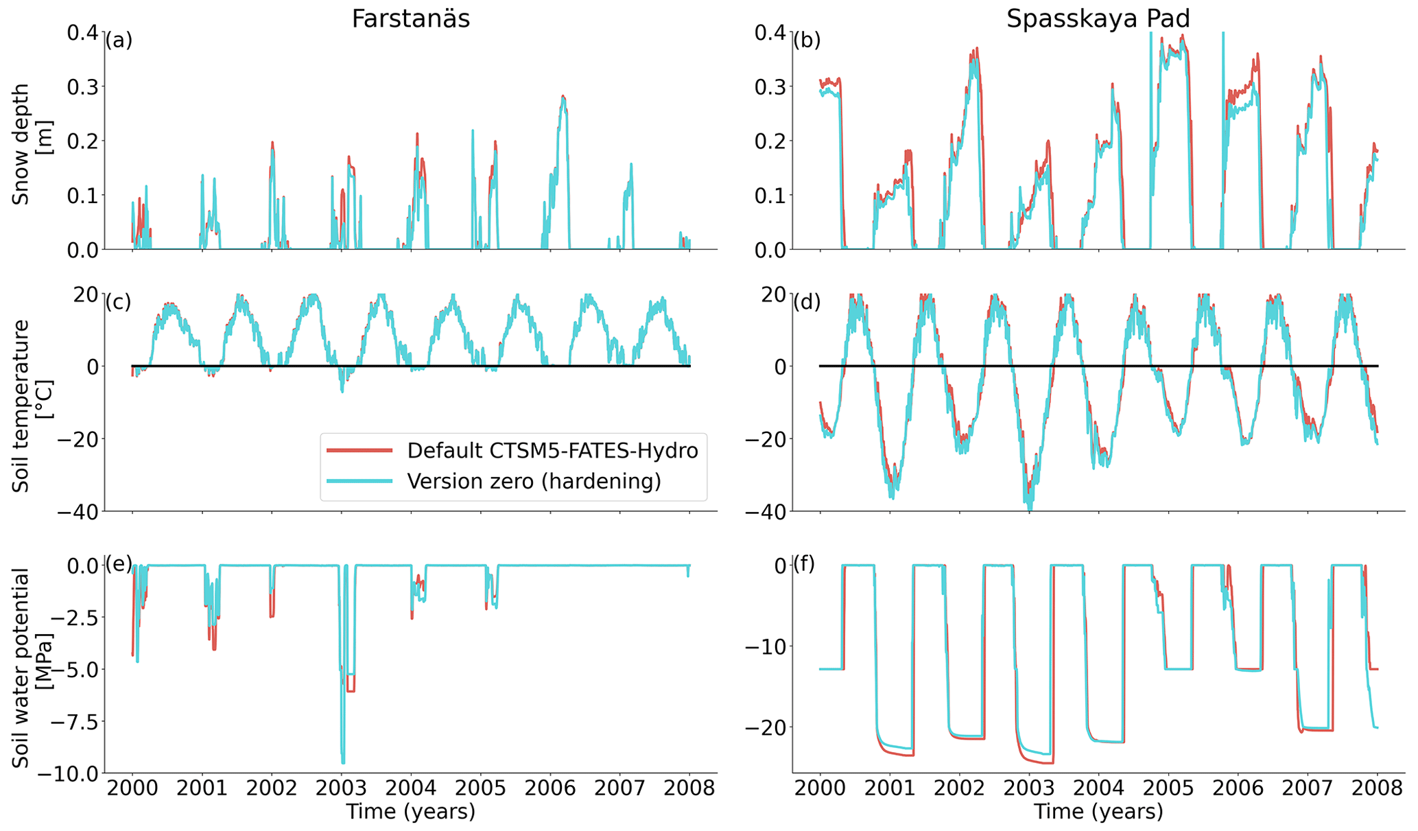
Figure 5Soil conditions for needleleaf evergreen trees at the sites of (a, c, and e) Farstanäs and (b, d, and f) Spasskaya Pad during the period 2000–2008. (a, b) Transpiration, (c, d) root water uptake, and (e, f) stored plant water. The default simulation is shown in red, and the hardening simulation is shown in blue.
2.4.4 Sensitivity experiments
To test the sensitivity of vegetation growth to the amplitude at which KMAX, g0 and g1, and HFM are modified by hardening, we tested individual modifications for each of these parameters (Table 2). Compared to the magnitude of the reductions selected in the version zero simulation, we selected both stronger and weaker reductions for the sensitivity experiments. Additional simulations were run to assess the impact of g0 and g1 independently from each other. We further tested extra implications which cold acclimation may have for processes in FATES-Hydro, such as the modification of PV curves and the reduction of CSM with hardening (Table 2). For CSM, the reductions with hardiness follow the same method as for HFM (Eq. 12). In contrast to the other CSM experiments, the one called “50 % all year” does not depend on the hardiness level but directly on HMAX instead. Two additional sensitivity experiments were performed on the temperature range of the dehardening rate (DR) and on the maximum hardiness level (HMAX) – parameters involved in the calculation of the hardiness level (Table 2). To evaluate the sensitivity of the hardening scheme to DR, we ran an experiment wherein the DR function increases between 0∘ and 10 ∘C and an experiment wherein DR increases between 5 and 15 ∘C (Table 2). While HMAX is defined as T5 minus 10 ∘C in the version zero simulation, we ran experiments wherein HMAX was defined by T5 minus 5 ∘C and T5 minus 15 ∘C.
3.1 Hardening to survive in the Arctic
At full spin-up, the default CLM5.0-FATES-Hydro model, without hardening, yielded evergreen tree biomass of ∼ 40 Mg C ha−1 at Farstanäs and only ∼ 0.2 Mg C ha−1 at Spasskaya Pad (Fig. 4a and b). After inclusion of the hardening scheme, larger biomass levels are simulated in Spasskaya Pad (∼ 4.5 Mg C ha−1) and similar levels at Farstanäs (∼ 42 Mg C ha−1).
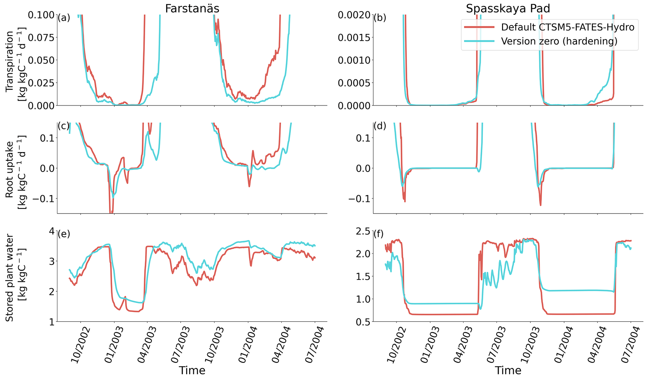
Figure 6Plant water fluxes for needleleaf evergreen trees at the sites of (a, c, and e) Farstanäs and (b, d, and f) Spasskaya Pad during the period September 2002–July 2004. (a, b) Transpiration, (c, d) root water uptake, and (e, f) stored plant water. The default simulation is shown in red, and the hardening simulation is shown in blue.

Figure 7Absorbing root water potential for needleleaf evergreen trees at the sites of (a) Farstanäs and (b) Spasskaya Pad during the period 2000–2008. The default simulation is shown in red, and the hardening simulation is shown in blue.
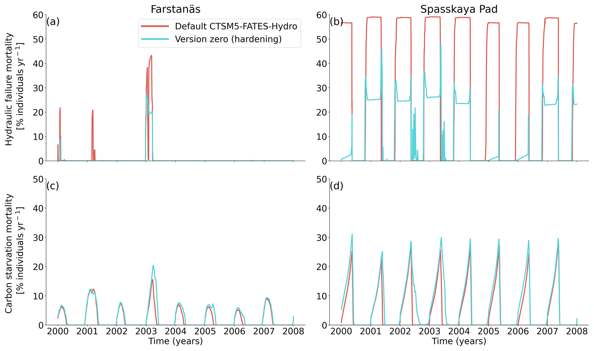
Figure 8Mortality rates for evergreen needleleaf trees at the sites of (a, c) Farstanäs and (b, d) Spasskaya Pad during the period 2000–2008. (a, b) Hydraulic failure mortality and (c, d) carbon starvation mortality. The default simulation is shown in red, and the hardening simulation is shown in blue.
In Spasskaya Pad, the temperature of the topsoil layers drops below −20 ∘C each winter (Fig. 5d). The resulting low liquid water content of the soil leads to such low matric potentials that the default model systematically simulates a release of water from the plant to the frozen soil (Fig. 6d). The root water release is strongest in autumn when soils start to freeze, but it can continue deep into the winter as long as plants still have stored water and the soil matric potential decreases further. If the topsoil temperature remains higher than −25 ∘C, our results show that winter dehydration typically leads to plant matric potentials higher than −15 MPa (Fig. 7b). During extreme years with topsoil temperatures below −25 ∘C, the matric potential in plant tissues can sometimes get as low as −28 MPa. The repetition of long-lasting low soil matric potentials one winter after the other resulted in large HFM rates (> 55 % individuals per year) (Fig. 8a and b). The sum of HFM, CSM, and other minor mortalities outweighs the summer productivity of needleleaf trees in Spasskaya Pad (Figs. 4b and S4b in the Supplement).
When the hardening model is employed in FATES-Hydro, low winter temperatures at Spasskaya Pad mean that HD quickly reaches the fixed limit of −70 ∘C (Fig. 10). This results in a strong reduction of (I) KMAX, (II) g0 and g1, and (III) HFM (see the Methods section above and “Sensitivity experiments” section below). The reduction of KMAX between tissues, and especially between absorbing roots and the first rhizosphere, greatly reduces the amplitude of reverse water flow through the roots when soils are frozen (Fig. 5c and d).
The temporal dynamics of the hardening model allow for cold-induced damage. For example, if temperatures abruptly drop below freezing in autumn, plants will not have acclimated yet and the amplitude of the reverse water flux will therefore be similar to the default model. However, as plants start acclimating, the resistance to water flux increases and root water exudation is inhibited by the hardening scheme. The second implication of hardening in our hydraulically adapted hardening scheme for plants is the reduction of g0 and g1. This reduces transpiration in spring and enables leaves to maintain their water potential while plants are still cold-acclimated. The reduction of the conductances (KMAX, g0, and g1) results in larger amounts of stored plant water (Fig. 6f). Levels of stored plant water are ∼ 2.4 kg (kg C)−1 during summer decrease to around ∼ 1.75 kg (kg C)−1 during warmer winters and reach as low as ∼ 1.1 kg (kg C)−1 during extremely cold winters. In the default model, stored water drops to ∼ 0.6 kg (kg C)−1 without major variation between years. By keeping larger amounts of water in hardened plants, the fractional loss of total conductance (flc) remains lower than in default simulations. The hardening scheme greatly reduces hydraulic failure mortality (HFM) at Spasskaya Pad (Fig. 8b), since HFM is a function of flc (Eq. 10), and an additional direct reduction of HFM was applied during cold acclimation (Fig. S12b in the Supplement). The contribution of hardiness to the reduction of KMAX, g0 and g1, and HFM can be seen by comparing Figs. 8b and S12. The changes imposed through hardening favors vegetation growth in northern regions, while the default model simulates almost nonexistent and declining vegetation (Fig. 4b).
At Farstanäs, temperatures in the topsoil layers usually remain between 0 and −5 ∘C during winter (Fig. 5c). This means that the water potential in plant compartments rarely drops below −3 MPa during typical winters. During cold winters, plant water potentials remain above −6 MPa in both the default and the hardening versions of the model (Fig. 7a). Therefore, the rate of HFM is lower at Farstanäs than at Spasskaya Pad, and episodes of mortality are shorter (Fig. 8a). In the simulations with hardening, plants have higher water potentials, reflective of the lower rates of water loss from winter root water exudation and stomatal transpiration. The main reason why the changes induced by hardening are small in Farstanäs – compared to Spasskaya Pad – is that changes are proportional to HD, which does not decrease much at Farstanäs (Fig. 10), and therefore the reductions applied to the conductance and mortality are smaller.
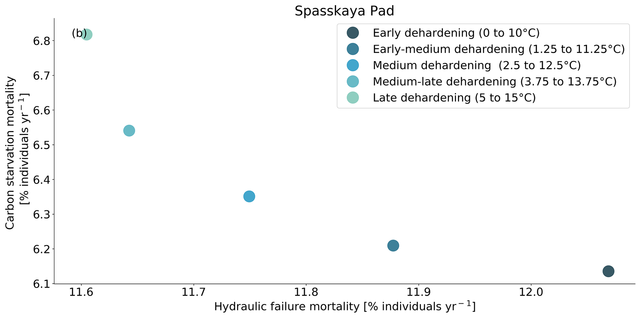
Figure 9Trade-off between hydraulic failure mortality and carbon starvation mortality for evergreen needleleaf trees at Spasskaya Pad for five dehardening sensitivity experiments. The mortality rates are averaged over the 30-year period 1981 to 2011.
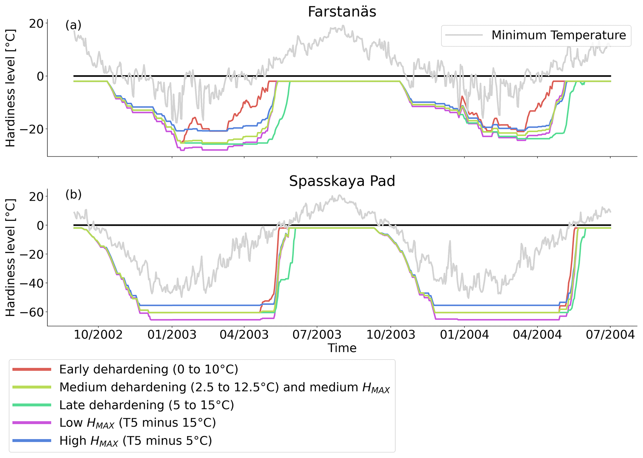
Figure 10Hardiness level from dehardening and maximum hardiness level sensitivity analysis simulations for needleleaf evergreen trees at the sites of (a) Farstanäs and (b) Spasskaya Pad during the period September 2002–July 2004. The grey line corresponds to the minimum daily temperature, the black line is 0 ∘C, and the colored lines are the dehardening and maximum level hardiness sensitivity experiments.
The simulations at Spasskaya Pad and Farstanäs both feature years with notably large drops in living biomass (Fig. 4a and b). These are related to low soil water potentials during winter (Fig. 7a and b). The unusually low soil matric potentials in these years contribute to an increase in dehydration and lead to higher mortality rates (Fig. 8). Our results show that a stronger reduction of KMAX with hardening, a lower HMAX, or a stronger reduction in HFM led to larger survival rates. At Spasskaya Pad, none of the sensitivity simulations prevented the strong mortality rates during extreme years (Fig. 11). While an even stronger reduction of KMAX and a later dehardening slightly helped survival, all simulations went through approximatively 50 % less mortality during the dry years. Figures S2b and 4b illustrate that during these extreme years, the total precipitation was low and the snow layer was thin. The water stored in plants and the matric potential of plants recovered only in the middle of the following summer (Figs. 6f and 7b).
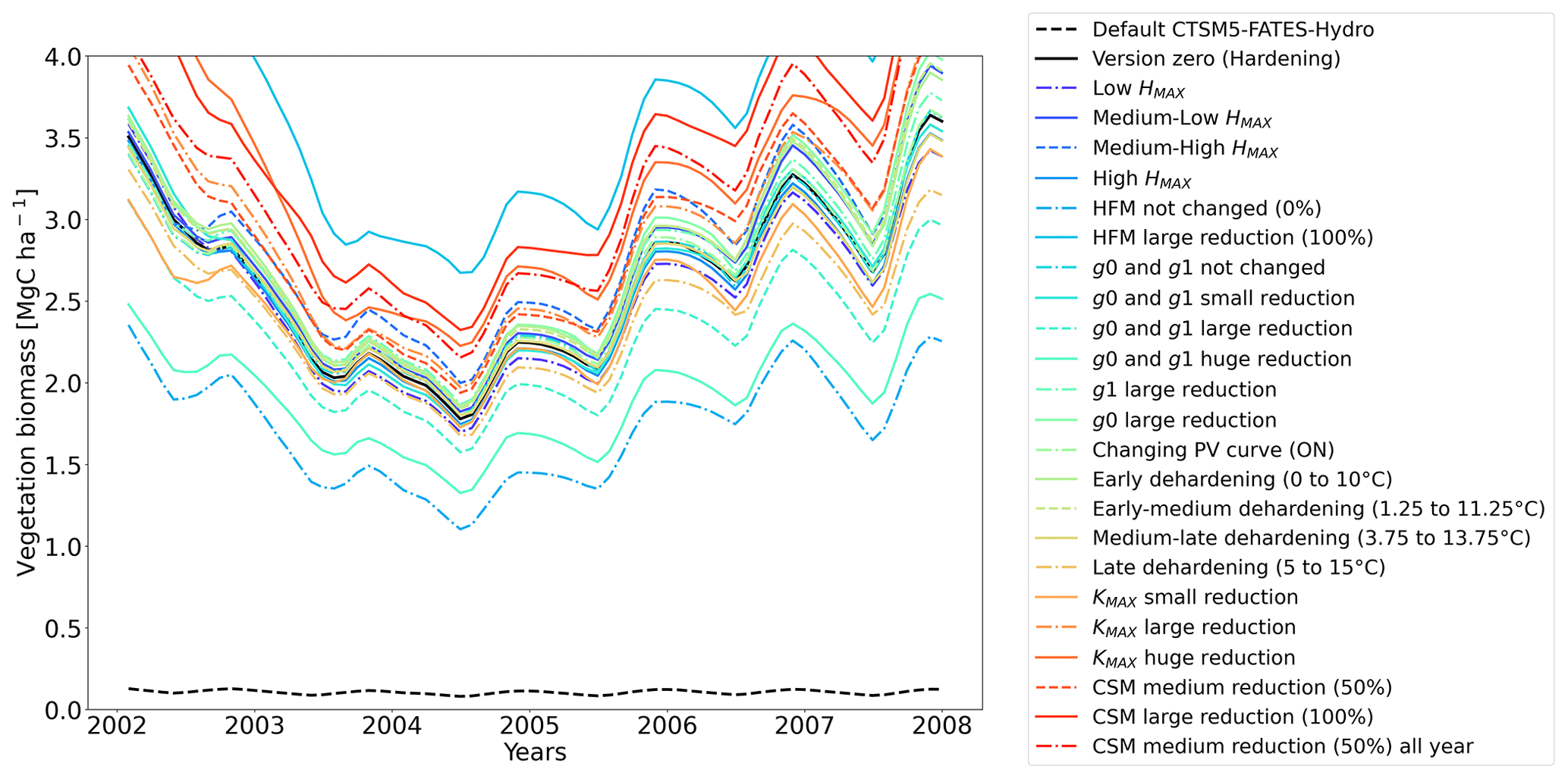
Figure 11Ensemble of living biomass simulations for needleleaf evergreen trees at the site of Spasskaya Pad during the period 2002–2008.
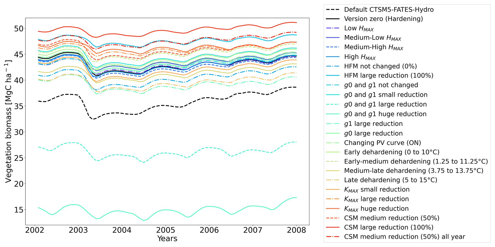
Figure 12Ensemble of living biomass simulations for needleleaf evergreen trees at the site of Farstanäs during the period 2002–2008.
3.2 Sensitivity experiments
3.2.1 Dehardening rate (DR)
At both sites (Farstanäs and Spasskaya Pad), the earlier dehardening starts, the better it is for vegetation growth (Figs. 11 and 12). There seem to be limited benefits in delaying hardening in autumn. At Spasskaya Pad, the modification of dehardening has little influence in the middle of the winter because of the extremely low hardiness levels (HD) (Fig. 10b). However, the “early dehardening simulation”, in which hardening decreases later and increases earlier (DR between 0 and 10 ∘C), shows root water efflux at the beginning and at the end of the winter season (Fig. S4d). This results in lower stored plant water and thereby higher hydraulic failure mortality (Figs. S4f and S5b in the Supplement). Interestingly, this results in a trade-off with carbon starvation mortality, since plant metabolism is activated earlier, reducing CSM (Fig. 9) and increasing gross primary productivity (Fig. S6 in the Supplement).
At Farstanäs, soils are rarely frozen in autumn and spring, and when they freeze it is never as much as in Spasskaya Pad (Fig. 5). This, combined with the shorter cold seasons and the higher hardiness levels during winter, results in a reduced occurrence of hydraulic failure mortality compared to Spasskaya Pad (Fig. S5). The 30-year atmospheric forcing period is too short and variable to show the trade-off between hydraulic failure mortality and carbon starvation mortality or even gross primary productivity.
3.2.2 Maximum hardiness level (HMAX)
At Spasskaya Pad, the HMAX sensitivity simulations (wherein HMAX is predicted by T5 minus variable Celsius degrees, see Table 1) are close to the hardening limit of −70 ∘C (Fig. 10b), which means that they yield similar results (Fig. 11).
At Farstanäs, lowering HMAX had large impacts on the total biomass (Fig. 12) because it increases survival during years with low soil water potentials and strong midwinter root water release (Fig. S5). Conversely, it reduces productivity during years with higher soil water potentials (Figs. S4 and 12).
In our model, a reduction in HMAX lowers conductivity, introducing a cost to plants in the form of decreased transpiration and photosynthesis (Fig. S4). Our results show the increase in CSM and decrease in HFM due to the lowering of HMAX at Spasskaya Pad (Fig. S7 in the Supplement).
3.2.3 Pressure–volume (PV) curve
PV curves were produced by making two of their parameters dependent on the hardening status HD (see the Methods section). Our implementation results in a shift in the PV curves when plants cold-acclimate and associates a lower matric potential with a given volumetric water content when they are hardened (Fig. 3). By decreasing the water potential in the plant, we effectively decrease the water gradient between freezing surface soil layers (generally surface layers). However, we simultaneously increase the water gradient between deep roots and unfrozen, usually deeper, soil layers. Since plants tend to establish equilibrium with the soil, stronger water uptake in deep roots decelerates the decrease in plant water potential.
Comparing Farstanäs and Spasskaya Pad reveals that the level of reduction of KMAX is crucial to the effective functioning of the dynamic PV curves. At Farstanäs (Fig. S8a in the Supplement), deep layers of the soil rarely freeze, and the weak reduction of KMAX enables water uptake, thereby offsetting the direct effect of HD on the PV curves. In Spasskaya Pad (Fig. S8b), the strong reduction in KMAX and the resulting prevention of water fluxes between roots and soil enabled lower water potential in the plant compartments. This led to slightly larger HFM rates and lower vegetation biomass (Fig. 11). We note that the higher leaf water potential in the dynamic PV simulation in Farstanäs in 2003 (Fig. S8a) is only due to differences in snow depths and changes to soil temperatures resulting from different biomasses between the two PV sensitivity simulations.
3.2.4 Maximum conductance between plant compartments (KMAX)
In this section, we show how sensitive evergreen trees are to the rate at which HD reduces KMAX (Eq. 7). In Farstanäs, weaker reductions of KMAX were favorable to vegetation productivity during “mild” winters, while stronger reductions became beneficial during “cold” winters (Fig. 12). During a cold year (e.g., first year of Fig. S9a, c, and e in the Supplement), the simulation with strong reduction in KMAX allows plants to lose less water to root exudation. Since trees hold onto more water, a larger exchange of water and carbon for photosynthesis is possible during early spring. By contrast, during a “mild” year (e.g., second year of Fig. S9a, c, and e), the strong reduction in KMAX does not provide an advantage for the plant since soil water potentials remain high and strong root water exudation is absent even in the default model run (Fig. 12). Again, our model captures the costs and benefits of hardening. Overall, it seems like the medium reduction of KMAX yields the highest biomass in Farstanäs (Fig. 12).
At Spasskaya Pad, large reductions in KMAX are always necessary to allow persistence of living biomass in our simulations (Fig. 11). Moreover, the simulations with the largest reductions of KMAX have the highest vegetation biomass.
3.2.5 Minimum stomatal conductance (g0 and g1)
Lowering g0 and g1 with hardening greatly reduces transpiration during winter (Fig. S10 in the Supplement). This allows leaf water potentials (Fig. S11 in the Supplement) to be maintained at values that do not trigger mortality. Reducing g0 and g1 also appears to lead to higher leaf water potentials during summer, especially at Farstanäs, potentially due to lower rates of transpiration resulting in larger water availability in the soil during summer (Fig. S10e and f). Overall, the reduction of g0 and g1 has a positive impact on the living biomass at both sites (Figs. 11 and 12).
Reducing only g0 leads to water loss when light levels increase the stomatal response, and reducing only g1 still allows substantial transpiration to occur when stomata are shut. Both need to be reduced to avoid a loss of internal plant water stores during wintertime (Fig. S11a and b).
3.2.6 Hydraulic failure mortality
If the rate scalar of HFM is not modified by the hardening scheme, high mortality rates are simulated for extended periods during winter at Spasskaya Pad (red line in Fig. S12b). When the rate of HFM is reduced by 50 % and 100 % at HMAX (green and light blue lines, respectively, in Fig. S12), this results in a large increase in vegetation biomass (Fig. 11). A 50 % reduction of HFM leads to almost a doubling of the biomass and a 100 % reduction (not realistic but included as an edge case) to almost a quadrupling.
On the other hand, the larger amounts of living biomass generated by the reduction of mortality imply that larger amounts of water are transpired and there is more competition for soil liquid water. During extreme years, it appears that vegetation in simulations with reduced HFM suffers from larger rates of CSM, which does not completely disappear during the following summer (Fig. S12d). In addition, while there was no HFM in the unchanged HFM simulation in spring, plants in reduced HFM simulations incur small amounts of HFM until later into the following summer (Fig. S12d).
3.2.7 Carbon starvation mortality
Implications of changing the rate of CSM are minor compared to HFM, although both scaling factors are identical (0.6 is the maximum mortality rate). HFM is parameterized in such a way that it quickly reaches 0.6 during strong water stress, while CSM remains at ∼ 0.3, even during the more extreme years (Fig. S13a and b in the Supplement). The biomass response of a reduction in CSM is similar at both sites: vegetation thrives best with reduced CSM (Figs. 11 and 12).
Much of the recent development of vegetation dynamics in land surface models has focused on representing advanced plant hydrodynamics (Christoffersen et al., 2016; Kennedy et al., 2019; Sperry et al., 2017; Xu et al., 2016). Usage of schemes that simulate the internal dynamics of plant moisture, however, has rarely been tested in cold systems – if at all, to our knowledge. By integrating a model of plant hardening with a porous media approach to plant hydrodynamics, we integrate a set of mechanisms that are both necessary for plants to avoid winter desiccation and capture the costs (in terms of reduced growth in spring) and benefits (in terms of reduced mortality rates) of winter “hardening”. Our analyses further highlight trade-offs between avoidance of “frost drought” mortality via hardening and avoidance of carbon starvation mortality via early-season photosynthesis.
The default version of the CLM5-FATES-Hydro model used here allows water to freeze in soils but not in plants. It does not include a mechanism to prevent liquid plant water from flowing from plants to soils when freezing strongly reduces soil water potential. We show that this results in a depletion of water in plant compartments and triggers large amounts of hydraulic failure and carbon starvation mortality.
The hydraulically mediated hardening scheme we propose in this paper consists of three modifications. The first is a reduction in the hydraulic conductivities of plant tissues, which inhibits or prevents water loss during freezing depending on the atmospheric temperatures and amount of hardening by the plants (Gusta et al., 2005; Smit-Spinks et al., 1984; Steponkus, 1984). While the benefit of hardening is the reduced hydraulic failure mortality during freezing soil events, its cost is a temporary reduction of photosynthesis due to reduced transpiration. The sensitivity experiments on the timing of dehardening (DR) and on the maximum hardiness level (HMAX) of this study highlight the considerable cost of hardening in cold sites which incur frequent hydraulic failure mortality (Figs. 9, S6 and S7). Previous field-based research has described the cost of hardening by showing that (1) cold acclimation causes a suppression of the rate of CO2 uptake (Krivosheeva et al., 1996), (2) low temperatures lead to the inhibition of sucrose synthesis and photosynthesis (Savitch et al., 2002; Stitt and Hurry, 2002), and (3) photosynthesis stops when needles freeze (Havranek and Tranquillini, 1995). In addition, growth cessation, dormancy, and cold acclimation are closely related to each other (Chang et al., 2021).
The second modification is to the stomatal model of Ball et al. (1987). Reducing g0 and g1 led to a slower decrease in leaf water potentials during late winter and spring, resulting in higher vegetation survival rates. We argue that the accompanying reduction in transpiration makes the model more realistic. Indeed, while photosynthesis is slightly influenced by cold in the default model, temperature is not taken into account in the calculation of transpiration, although the literature has shown that g0 and g1 are lower in cold-acclimated plants (Christersson, 1972; Duursma et al., 2019; James et al., 2008). A partial but not full reduction of g0 and g1 allows for some transpiration, thereby maintaining the capacity of the advanced hydraulic model to represent winter droughts. In contrast to summer droughts, typically caused by the absence of rainfall in summer, winter droughts or frost droughts are caused by the unavailability of water in frozen soils, preventing the replacement of transpired water during warm winter days.
The third modification that comprises our hardening scheme is the reduction in the rate of HFM. While the default formulation of HFM might be realistic when simulating summer droughts, it is not adapted to boreal and Arctic regions where winter droughts would cause extended periods of mortality (i.e., lasting until snowmelt in spring). At cold sites, the default CLM5-FATES-Hydro simulates a frost drought each winter due to root water exudation, which systematically results in maximum HFM rates from late autumn until spring snowmelt when soils finally thaw. The current parameterization of HFM in cold regions is such that summer productivity cannot balance the high winter mortality. In reality, high-latitude vegetation is dormant in winter and the metabolism of plants is reduced or completely interrupted (Volaire, 2018). When dormant, plants reduce or stop meristem activity to make it insensitive to growth and promote signals in order to enhance survival during seasons with life-threatening environmental conditions (Volaire, 2018). To quote Volaire (2018), “knowing when not to grow does not confer drought resistance but may well enhance drought survival”. Our results show that the reduction of HFM with hardening can lead to large increases in biomass in areas with cold winters. The large amounts of biomass, however, appear to be a limiting factor during dry years, when plants must compete for water. The larger amount of biomass caused by reduced HFM rates resulted in higher CSM rates, highlighting another trade-off emerging from the hardening scheme.
To tolerate freezing, plants undergo a set of physiological changes. The capacity to efficiently cold-acclimate and survive frost depends on a plant's genome and the presence of performant cold tolerance traits. Therefore, in reality different species may exhibit different maximum hardiness levels (HMAX), hardening rates (HR), dehardening rates (DR), and temperature ranges wherein hardening and dehardening occur (Mabaso et al., 2019; Oberschelp et al., 2020). In terrestrial biosphere models, species are aggregated in groups based on criteria for common functional characteristics. Therefore, it is likely that the measured maximum freezing tolerance of some species that are within the same plant functional type category in the model is variable in reality. (Sakai, 1983). A PFT's maximum freezing tolerance (as well as most parameters of terrestrial biosphere models) is a rough approximation of what has been measured for species belonging to that PFT. Common gardens are generally used to identify the genetic variations among populations in their ability to cope with stresses (Bansal et al., 2016; de Villemereuil et al., 2016). As the expression of physiological–morphological traits associated with stress tolerance is also dependent on the environmental conditions of a common garden, several gardens are required to quantify the relative influence of environment and genetics on the expression of stress tolerance traits (Greer and Warrington, 1982). Earlier studies used a HMAX of −30 ∘C and a DR initiated at 5 ∘C to model the hardiness of Norway spruce in Farstanäs (Bigras and Colombo, 2013; Jönsson et al., 2004; Rammig et al., 2010). However, Pinus sylvestris seedlings in Finland already start dehardening at temperatures as low as 3 ∘C (Repo and Pelkonen, 1986). Our hydraulically mediated hardening scheme captures both the costs and benefits of hardening, which in simulations with dynamic vegetation would likely lead to different competitive outcomes for plants with alternative hardening thresholds. Finer discretization of plant strategies along the axis of cold tolerance would provide an interesting extension to this study.
The physiological changes induced by cold acclimation result in modifications of the osmotic potential at full turgor and the bulk elastic modulus (Mart et al., 2016; Scholz et al., 2012; Valentini et al., 1990), i.e., two parameters that intervene in the calculation of the plant PV curves. In the changing PV curve simulation (see the Methods section for more details), lower winter root water exudation and transpiration fluxes were simulated. If KMAX is not low enough, larger root water uptake (especially in deeper layers that remain unfrozen longer in autumn) balances the decrease in plant water potential. While the PV curve modification should be a more realistic approach to model plant hydraulics, it also results in larger HFM and lower biomass.
Our study illustrated the potential for a trade-off between the avoidance of HFM in the spring and the avoidance of CSM triggered by low photosynthesis rates resulting from a long hardening season. This trade-off mirrors the one originally proposed by McDowell et al. (2008) for summer droughts (whereby stomatal closure avoids HFM but implies CSM). Mature trees store large amounts of mobile carbon, which decrease under water stress, but evidence to support this hypothesis is lacking (Hartmann, 2015; Sala, 2009). While HFM can be assessed by the percent loss of total conductance, CSM is much harder to infer. The limited understanding of the roles of non-structural carbohydrates suggests a link between CSM and HFM as sugars are not only a source of energy, but also regulate osmotic pressure and embolism repair following drought (McDowell and Sevanto, 2010). Our results show that changes in CSM result in relatively small changes in biomass compared to HFM reductions. This is mainly due to the fact that droughts typically cause larger HFM than CSM episodes.
In this study, we propose a hardening scheme adapted for use within the context of plant hydrodynamic simulations, which can simulate the physiological costs and benefits of plant cold acclimation in terms of water movement and gas exchange. Its impact on plant hydraulics as well as vegetation mortality and growth appears to be a promising improvement for the modeling of vegetation growth in cold environments. We present one parameterization of the hardening scheme, show how it performs at two sites with contrasting winter weather, and investigate the response of the scheme to variations to its key parameters. Although the understanding about cold acclimation processes is expanding at an accelerating rate, there are still large knowledge gaps. For example, the range of processes triggered by cold acclimation is poorly understood and we lack measurements to define the exact amplitude at which they are disturbed (Arora and Rowland, 2011; Chang et al., 2021; Shi et al., 2018; Shin et al., 2015). In addition, quantifying and generalizing hardiness levels and rates inside the scheme itself are in some respects broad approximations which remain to be optimized further. Future developments might, for example, consider a larger influence of photoperiod and the inclusion of plant phenological states in the calculation of the hardiness level. In this study, we primarily aim to discuss the role and impacts of major parameters as well as potential impacts of cold acclimation as a framework for further implementation in dynamic vegetation models with advanced plant hydraulics. We show (1) that this framework leads to more realistic vegetation biomass productivity at temperate and boreal sites, (2) that this framework influences winter root water release and mortality rates by lowering plant conductance, and (3) that hardening comes at a cost for photosynthesis (trade-off of hardening emerges from our scheme).
Recent observations of increasing vegetation mortality appear to be a result of climate change, in particular the increase in intensity and frequency of droughts caused by extreme weather conditions (Allen et al., 2010). This highlights the urgency to improve our understanding of plant survival and mortality mechanisms. To date, there are large gaps in our knowledge on plant hydraulics and their link to mortality rates. In this paper, we hope to provide new insights into modeling of plant hydraulics and their link to cold acclimation.
Future research is needed to better assess the implications of cold acclimation on plant hydraulics, especially conductivity. Understanding these processes in hampered by the logistical and technical difficulties involved in the observation of cold systems. Our work lays the foundation to use a hardening scheme to regulate frost damage and to study the link between different types of mortalities in terrestrial biosphere models in the Arctic region. The inclusion of cold hardiness is essential to model realistic plant hydraulics and vegetation dynamics within cold climates.
The modeling data that support the findings of this study are available at https://doi.org/10.11582/2022.00028 (Lambert, 2022). The code of CTSM5.0 can be found at https://doi.org/10.5281/zenodo.6559825 (CTSM Development Team, 2022) and the code of FATES at https://doi.org/10.5281/zenodo.6559840 (FATES Development Team, 2022).
The supplement related to this article is available online at: https://doi.org/10.5194/gmd-15-8809-2022-supplement.
MSAL, HT, KJA, FS, RAF, and FJWP designed the work; MSAL performed experiments and data analyses; MSAL drafted the paper; HT, KSA, FS, RAF, YF, JD, and FJWP revised the paper. All authors approved the final version of the paper for publication.
The contact author has declared that none of the authors has any competing interests.
Publisher's note: Copernicus Publications remains neutral with regard to jurisdictional claims in published maps and institutional affiliations.
This work is a contribution to the Strategic Research Initiative “Land Atmosphere Interactions in Cold Environments” (LATICE) of the University of Oslo. We gratefully acknowledge the support of the Research Council of Norway for WINTERPROOF (project no. 274711), the Swedish Research Council under registration no. 2017-05268, EMERALD (project no. 294948), and the Centre for Biogeochemistry in the Anthropocene at the Faculty of Mathematics and Natural Sciences at UiO. We would also like to thank the ECMWF for the ERA5L reanalysis product. Finally, we would like to acknowledge our colleagues at NCAR and Berkeley lab for their precious help during model setup and paper preparation. Rosie A. Fisher acknowledges the support of the US Department of Energy “Next Generation Ecosystem Experiment in the Tropics” project, and Rosie A. Fisher and Kjetil S. Aas acknowledge the support of the EUH2020 4C project. Yilin Fang acknowledges the support of the Energy Exascale Earth System Model (E3SM) project, funded by the US Department of Energy, Office of Science Biological and Environmental Research, through the Earth System Model Development program area. The Pacific Northwest National Laboratory is operated for DOE by Battelle Memorial Institute under contract DE-AC06-76RL01830. The simulations were performed on the FRAM supercomputer operated by Sigma2 (project number NN2806K).
This research has been supported by the Norges Forskningsråd (grant no. 274711), the Vetenskapsrådet (grant no. 2017-05268), EMERALD (project no. 294948), and the EUH2020 4C project (grant no. 821003).
This paper was edited by Hisashi Sato and reviewed by Tim Artlip and one anonymous referee.
Allen, C. D., Macalady, A., Chenchouni, H., Bachelet, D., McDowell, N., Vennetier, M., Gonzales, P., Hogg, T., Rigling, A., and Breshears, D.: Climate-induced forest mortality: a global overview of emerging risks, Forest Ecol. Manag., 259, 660–684, 2010.
Arora, R. and Rowland, L. J.: Physiological research on winter-hardiness: deacclimation resistance, reacclimation ability, photoprotection strategies, and a cold acclimation protocol design, HortScience, 46, 1070–1078, 2011.
Ball, J. T., Woodrow, I. E., and Berry, J. A.: A Model Predicting Stomatal Conductance and its Contribution to the Control of Photosynthesis under Different Environmental Conditions, in: Progress in Photosynthesis Research, edited by: Biggins, J., Springer, Dordrecht, https://doi.org/10.1007/978-94-017-0519-6_48, 1987.
Bansal, S., Harrington, C. A., and St. Clair, J. B.: Tolerance to multiple climate stressors: A case study of Douglas-fir drought and cold hardiness, Ecol. Evol., 6, 2074–2083, 2016.
Bartlett, M. K., Scoffoni, C., and Sack, L.: The determinants of leaf turgor loss point and prediction of drought tolerance of species and biomes: a global meta-analysis, Ecol. Lett., 15, 393–405, 2012.
Beck, E. H., Heim, R., and Hansen, J.: Plant resistance to cold stress: mechanisms and environmental signals triggering frost hardening and dehardening, J. Bioscience., 29, 449–459, 2004.
Beck, E. H., Fettig, S., Knake, C., Hartig, K., and Bhattarai, T.: Specific and unspecific responses of plants to cold and drought stress, J. Bioscience., 32, 501–510, 2007.
Bigras, F. J. and Colombo, S. J.: Conifer cold hardiness, edited by: Bigras, F. J. and Colombo S. J., Springer Dordrecht, https://doi.org/10.1007/978-94-015-9650-3, 2013.
Bonan, G. B., Williams, M., Fisher, R. A., and Oleson, K. W.: Modeling stomatal conductance in the earth system: linking leaf water-use efficiency and water transport along the soil–plant–atmosphere continuum, Geosci. Model Dev., 7, 2193–2222, https://doi.org/10.5194/gmd-7-2193-2014, 2014.
Campbell, G. S.: A simple method for determining unsaturated conductivity from moisture retention data, Soil Sci., 117, 311–314, 1974.
Carminati, A., Vetterlein, D., Weller, U., Vogel, H.-J., and Oswald, S. E.: When roots lose contact, Vadose Zone J., 8, 805–809, 2009.
Chang, C. Y.-Y., Bräutigam, K., Hüner, N. P., and Ensminger, I.: Champions of winter survival: cold acclimation and molecular regulation of cold hardiness in evergreen conifers, New Phytol., 229, 675–691, 2021.
Chinnusamy, V., Zhu, J., and Zhu, J.-K.: Gene regulation during cold acclimation in plants, Physiol. Plantarum, 126, 52–61, 2006.
Christersson, L.: The transpiration rate of unhardened, hardened, and dehardened seedlings of spruce and pine, Physiol. Plantarum, 26, 258–263, 1972.
Christoffersen, B. O., Gloor, M., Fauset, S., Fyllas, N. M., Galbraith, D. R., Baker, T. R., Kruijt, B., Rowland, L., Fisher, R. A., Binks, O. J., Sevanto, S., Xu, C., Jansen, S., Choat, B., Mencuccini, M., McDowell, N. G., and Meir, P.: Linking hydraulic traits to tropical forest function in a size-structured and trait-driven model (TFS v.1-Hydro), Geosci. Model Dev., 9, 4227–4255, https://doi.org/10.5194/gmd-9-4227-2016, 2016.
Clapp, R. B. and Hornberger, G. M.: Empirical equations for some soil hydraulic properties, Water Resour. Res., 14, 601–604, 1978.
CTSM Development Team: mariuslam/PAPER1_CTSM: PAPER1_CTSM (Version V1), Zenodo [code], https://doi.org/10.5281/zenodo.6559825, 2022. a
Darcy, H.: Les fontaines publiques de la ville de Dijon: exposition et application…, Victor Dalmont, Paris, France, 1856.
de Villemereuil, P., Gaggiotti, O. E., Mouterde, M., and Till-Bottraud, I.: Common garden experiments in the genomic era: new perspectives and opportunities, Heredity, 116, 249–254, 2016.
Ding, Y., Zhang, Y., Zheng, Q.-S., and Tyree, M. T.: Pressure–volume curves: revisiting the impact of negative turgor during cell collapse by literature review and simulations of cell micromechanics, New Phytol., 203, 378–387, 2014.
Dowgert, M. F. and Steponkus, P. L.: Behavior of the plasma membrane of isolated protoplasts during a freeze-thaw cycle, Plant Physiol., 75, 1139–1151, 1984.
Duursma, R. A. and Medlyn, B. E.: MAESPA: a model to study interactions between water limitation, environmental drivers and vegetation function at tree and stand levels, with an example application to [CO2] × drought interactions, Geosci. Model Dev., 5, 919–940, https://doi.org/10.5194/gmd-5-919-2012, 2012.
Duursma, R. A., Blackman, C. J., Lopéz, R., Martin-StPaul, N. K., Cochard, H., and Medlyn, B. E.: On the minimum leaf conductance: its role in models of plant water use, and ecological and environmental controls, New Phytol., 221, 693–705, 2019.
Edwards, W. R. N., Jarvis, P. G., Landsberg, J. J., and Talbot, H.: A dynamic model for studying flow of water in single trees, Tree Physiol., 1, 309–324, 1986.
FATES Development Team: The Functionally Assembled Terrestrial Ecosystem Simulator (FATES) (Version v1), Zenodo [code], https://doi.org/10.5281/zenodo.6559840, 2022. a
Fisher, R. A., Muszala, S., Verteinstein, M., Lawrence, P., Xu, C., McDowell, N. G., Knox, R. G., Koven, C., Holm, J., Rogers, B. M., Spessa, A., Lawrence, D., and Bonan, G.: Taking off the training wheels: the properties of a dynamic vegetation model without climate envelopes, CLM4.5(ED), Geosci. Model Dev., 8, 3593–3619, https://doi.org/10.5194/gmd-8-3593-2015, 2015.
Fontes, C.: Tropical plant hydraulics in a changing climate: importance for species distribution and vulnerability to drought, University of California, Berkeley, 2019.
Fricke, W.: Turgor pressure, in: eLS, Wiley & Sons, Ltd, Chichester, 1–6, https://doi.org/10.1002/9780470015902.a0001687.pub2, 2017.
Greenwood, S., Ruiz-Benito, P., Martínez-Vilalta, J., Lloret, F., Kitzberger, T., Allen, C. D., Fensham, R., Laughlin, D. C., Kattge, J., and Bönisch, G.: Tree mortality across biomes is promoted by drought intensity, lower wood density and higher specific leaf area, Ecol. Lett., 20, 539–553, 2017.
Greer, D. H. and Warrington, I. J.: Effect of photoperiod, night temperature, and frost incidence on development of frost hardiness in Pinus radiata, Funct. Plant Biol., 9, 333–342, 1982.
Gusta, L. V., Trischuk, R., and Weiser, C. J.: Plant cold acclimation: the role of abscisic acid, J. Plant Growth Regul., 24, 308–318, 2005.
Hamada, S., Ohta, T., Hiyama, T., Kuwada, T., Takahashi, A., and Maximov, T. C.: Hydrometeorological behaviour of pine and larch forests in eastern Siberia, Hydrol. Process., 18, 23–39, 2004.
Hanin, M., Brini, F., Ebel, C., Toda, Y., Takeda, S., and Masmoudi, K.: Plant dehydrins and stress tolerance: versatile proteins for complex mechanisms, Plant Signaling & Behavior, 6, 1503–1509, 2011.
Hartmann, H.: Carbon starvation during drought-induced tree mortality–are we chasing a myth?, Journal of Plant Hydraulics, 2, e005, https://doi.org/10.20870/jph.2015.e005, 2015.
Havranek, W. M. and Tranquillini, W.: Physiological processes during winter dormancy and their ecological significance, in: Ecophysiology of coniferous forests, edited by: Smith, W. K. and Hinckley, T. M., Elsevier, 95–124, ISBN 9780080925936, https://doi.org/10.1016/B978-0-08-092593-6.50010-4, 1995.
Isaev, A. P., Protopopov, A. V., Protopopova, V. V., Egorova, A. A., Timofeyev, P. A., Nikolaev, A. N., Shurduk, I. F., Lytkina, L. P., Ermakov, N. B., and Nikitina, N. V.: Vegetation of Yakutia: Elements of Ecology and Plant Sociology, in: The Far North. Plant and Vegetation, vol 3., edited by: Troeva, E., Isaev, A., Cherosov, M., and Karpov, N., Springer, Dordrecht, 143–260, https://doi.org/10.1007/978-90-481-3774-9_3, 2010.
James, A. T., Lawn, R. J., and Cooper, M.: Genotypic variation for drought stress response traits in soybean. I. Variation in soybean and wild Glycine spp. for epidermal conductance, osmotic potential, and relative water content, Aust. J. Agr. Res., 59, 656–669, 2008.
Janská, A., Maršík, P., Zelenková, S., and Ovesná, J.: Cold stress and acclimation – what is important for metabolic adjustment?, Plant Biol., 12, 395–405, 2010.
Jarvis, P. G. and Morison, J. I. L.: The control of transpiration and photosynthesis by the stomata, in: Stomatal physiology, vol. 8, edited by: Jarvis, P. G. and Mansfield, T. A., Cambridge University Press Cambridge, UK, 247–279, ISBN 0-521-23683-5 (hard cover), ISBN 0-521-23151-2 (paperback), 1981.
Jönsson, A. M., Linderson, M.-L., Stjernquist, I., Schlyter, P., and Bärring, L.: Climate change and the effect of temperature backlashes causing frost damage in Picea abies, Global Planet. Change, 44, 195–207, 2004.
Kellomaki, S., Hanninen, H., and Kolstrom, M.: Computations on frost damage to Scots pine under climatic warming in boreal conditions, Ecol. Appl., 5, 42–52, 1995.
Kennedy, D., Swenson, S., Oleson, K. W., Lawrence, D. M., Fisher, R., Lola da Costa, A. C., and Gentine, P.: Implementing plant hydraulics in the community land model, version 5, J. Adv. Model. Earth Sy., 11, 485–513, 2019.
Knipfer, T., Besse, M., Verdeil, J.-L., and Fricke, W.: Aquaporin-facilitated water uptake in barley (Hordeum vulgare L.) roots, J. Exp. Bot., 62, 4115–4126, 2011.
Koven, C.: FATES Parameters and Output for Parameter Sensitivity at the Panama Barro Colorado Island Testbed, Next-Generation Ecosystem Experiments Tropics; Lawrence Berkeley National, USA, https://doi.org/10.15486/ngt/1569647, 2019.
Kreszies, T., Shellakkutti, N., Osthoff, A., Yu, P., Baldauf, J. A., Zeisler-Diehl, V. V., Ranathunge, K., Hochholdinger, F., and Schreiber, L.: Osmotic stress enhances suberization of apoplastic barriers in barley seminal roots: analysis of chemical, transcriptomic and physiological responses, New Phytol., 221, 180–194, https://doi.org/10.1111/nph.15351, 2019.
Krivosheeva, A., Tao, D.-L., Ottander, C., Wingsle, G., Dube, S. L., and Öquist, G.: Cold acclimation and photoinhibition of photosynthesis in Scots pine, Planta, 200, 296–305, 1996.
Kuprian, E., Koch, S., Munkler, C., Resnyak, A., Buchner, O., Oberhammer, M., and Neuner, G.: Does winter desiccation account for seasonal increases in supercooling capacity of Norway spruce bud primordia?, Tree Physiol., 38, 591–601, 2018.
Kursar, T. A., Engelbrecht, B. M., Burke, A., Tyree, M. T., EI Omari, B., and Giraldo, J. P.: Tolerance to low leaf water status of tropical tree seedlings is related to drought performance and distribution, Funct. Ecol., 23, 93–102, 2009.
Lambert, M.: PAPER1: cold hardening scheme, Norstore [data set], https://doi.org/10.11582/2022.00028, 2022. a
Lawrence, D. M., Fisher, R. A., Koven, C. D., et al.: The Community Land Model version 5: Description of new features, benchmarking, and impact of forcing uncertainty, J. Adv. Model. Earth Sy., 11, 4245–4287, 2019.
Lee, S., Chung, G. C., and Steudle, E.: Low temperature and mechanical stresses differently gate aquaporins of root cortical cells of chilling-sensitive cucumber and-resistant figleaf gourd, Plant Cell Environ., 28, 1191–1202, 2005.
Levitt, J.: Responses of Plants to Environmental Stress, Volume 1: Chilling, Freezing, and High Temperature Stresses, Academic Press, ISBN 9780124455016, 1980.
Li, C., Junttila, O., and Palva, E. T.: Environmental regulation and physiological basis of freezing tolerance in woody plants, Acta Physiol. Plant., 26, 213–222, 2004.
Lopez-Iglesias, B., Villar, R., and Poorter, L.: Functional traits predict drought performance and distribution of Mediterranean woody species, Acta Oecol., 56, 10–18, 2014.
Mabaso, F., Ham, H., and Nel, A.: Frost tolerance of various Pinus pure species and hybrids, South. Forests, 81, 273–280, 2019.
Manzoni, S., Vico, G., Katul, G., Palmroth, S., Jackson, R. B., and Porporato, A.: Hydraulic limits on maximum plant transpiration and the emergence of the safety–efficiency trade-off, New Phytol., 198, 169–178, 2013.
Mart, K. B., Veneklaas, E. J., and Bramley, H.: Osmotic potential at full turgor: an easily measurable trait to help breeders select for drought tolerance in wheat, Plant Breeding, 135, 279–285, 2016.
McDowell, N., Pockman, W. T., Allen, C. D., Breshears, D. D., Cobb, N., Kolb, T., Plaut, J., Sperry, J., West, A., Williams, D. G., and Yepez, E. A.: Mechanisms of plant survival and mortality during drought: why do some plants survive while others succumb to drought?, New Phytol., 178, 719–739, 2008.
McDowell, N. G. and Sevanto, S.: The mechanisms of carbon starvation: how, when, or does it even occur at all?, New Phytol., 186, 264–266, 2010.
Mirfenderesgi, G., Bohrer, G., Matheny, A. M., Fatichi, S., de Moraes Frasson, R. P., and Schäfer, K. V.: Tree level hydrodynamic approach for resolving aboveground water storage and stomatal conductance and modeling the effects of tree hydraulic strategy, J. Geophys. Res.-Biogeo., 121, 1792–1813, 2016.
Muñoz Sabater, J.: ERA5-Land hourly data from 1981 to present, Copernicus Climate Change Service (C3S) Climate Data Store (CDS) [data set], https://doi.org/10.24381/cds.e2161bac, 2019.
Nadezhdina, N., David, T. S., David, J. S., Ferreira, M. I., Dohnal, M., Tesař, M., Gartner, K., Leitgeb, E., Nadezhdin, V., Cermak, J., Soledad Jimenez, M., and Morales, D.: Trees never rest: the multiple facets of hydraulic redistribution, Ecohydrology, 3, 431–444, 2010.
Navarro, M. Á. P., Sapes, G., Batllori, E., Serra-Diaz, J. M., Esteve, M. A., and Lloret, F.: Climatic suitability derived from species distribution models captures community responses to an extreme drought episode, Ecosystems, 22, 77–90, 2019.
North, G. B. and Nobel, P. S.: Hydraulic conductivity of concentric root tissues of Agave deserti Engelm. under wet and drying conditions, New Phytol., 130, 47–57, 1995.
North, G. B. and Nobel, P. S.: Root-soil contact for the desert succulent Agave deserti in wet and drying soil, New Phytol., 135, 21–29, 1997.
Oberschelp, G. P. J., Guarnaschelli, A. B., Teson, N., Harrand, L., Podestá, F. E., and Margarit, E.: Cold acclimation and freezing tolerance in three Eucalyptus species: A metabolomic and proteomic approach, Plant Physiol. Bioch., 154, 316–327, 2020.
Oliveira, R. S., Dawson, T. E., Burgess, S. S., and Nepstad, D. C.: Hydraulic redistribution in three Amazonian trees, Oecologia, 145, 354–363, 2005.
Petrov, K. A., Sofronova, V. E., Bubyakina, V. V., Perk, A. A., Tatarinova, T. D., Ponomarev, A. G., Chepalov, V. A., Okhlopkova, Z. M., Vasilieva, I. V., and Maximov, T. C.: Woody plants of Yakutia and low-temperature stress, Russ. J. Plant Physl.+, 58, 1011–1019, 2011.
Prieto, I., Armas, C., and Pugnaire, F. I.: Water release through plant roots: new insights into its consequences at the plant and ecosystem level, New Phytol., 193, 830–841, 2012.
Rammig, A., Jönsson, A. M., Hickler, T., Smith, B., Bärring, L., and Sykes, M. T.: Impacts of changing frost regimes on Swedish forests: incorporating cold hardiness in a regional ecosystem model, Ecol. Model., 221, 303–313, 2010.
Rasztovits, E., Berki, I., Mátyás, C., Czimber, K., Pötzelsberger, E., and Móricz, N.: The incorporation of extreme drought events improves models for beech persistence at its distribution limit, Ann For. Sci., 71, 201–210, 2014.
Repo, T. and Pelkonen, P.: Temperature step response of dehardening in Pinus sylvestris seedlings, Scand. J. Forest Res., 1, 271–284, 1986.
Rinne, P., Welling, A., and Kaikuranta, P.: Onset of freezing tolerance in birch (Betula pubescens Ehrh.) involves LEA proteins and osmoregulation and is impaired in an ABA‐deficient genotype, Plant Cell Environ., 21, 601–611, 1998.
Sakai, A.: Comparative study on freezing resistance of conifers with special reference to cold adaptation and its evolutive aspects, Can. J. Botany, 61, 2323–2332, 1983.
Sala, A.: Lack of direct evidence for the carbon-starvation hypothesis to explain drought-induced mortality in trees, P. Natl. Acad. Sci. USA, 106, E68–E68, 2009.
Sato, H., Kobayashi, H., and Delbart, N.: Simulation study of the vegetation structure and function in eastern Siberian larch forests using the individual-based vegetation model SEIB-DGVM, Forest Ecol. Manag., 259, 301–311, 2010.
Savitch, L. V., Leonardos, E. D., Krol, M., Jansson, S., Grodzinski, B., Huner, N. P. A., and Öquist, G.: Two different strategies for light utilization in photosynthesis in relation to growth and cold acclimation, Plant Cell Environ., 25, 761–771, 2002.
Scholz, F. G., Bucci, S. J., Arias, N., Meinzer, F. C., and Goldstein, G.: Osmotic and elastic adjustments in cold desert shrubs differing in rooting depth: coping with drought and subzero temperatures, Oecologia, 170, 885–897, 2012.
Shi, Y., Ding, Y., and Yang, S.: Molecular regulation of CBF signaling in cold acclimation, Trends Plant Sci., 23, 623–637, 2018.
Shin, H., Oh, Y., and Kim, D.: Differences in cold hardiness, carbohydrates, dehydrins and related gene expressions under an experimental deacclimation and reacclimation in Prunus persica, Physiol. Plantarum, 154, 485–499, https://doi.org/10.1111/ppl.12293, 2015.
Smit-Spinks, B., Swanson, B. T., and Markhart, A. I.: Changes in water relations, water flux, and root exudate abscisic acid content with cold acclimation of Pinus sylvestris L, Funct. Plant Biol., 11, 431–441, 1984.
Sperry, J., Adler, F., Campbell, G., and Comstock, J.: Limitation of plant water use by rhizosphere and xylem conductance: results from a model, Plant Cell Environ., 21, 347–359, 1998.
Sperry, J. S., Venturas, M. D., Anderegg, W. R., Mencuccini, M., Mackay, D. S., Wang, Y., and Love, D. M.: Predicting stomatal responses to the environment from the optimization of photosynthetic gain and hydraulic cost, Plant Cell Environ., 40, 816–830, 2017.
Steponkus, P. L.: Role of the plasma membrane in freezing injury and cold acclimation, Annu. Rev. Plant Physio., 35, 543–584, 1984.
Stitt, M. and Hurry, V.: A plant for all seasons: alterations in photosynthetic carbon metabolism during cold acclimation in Arabidopsis, Curr. Opin. Plant Biol., 5, 199–206, 2002.
Sugimoto, A., Yanagisawa, N., Naito, D., Fujita, N., and Maximov, T. C.: Importance of permafrost as a source of water for plants in east Siberian taiga, Ecol. Res., 17, 493–503, 2002.
Tatarinova, T. D., Perk, A. A., Bubyakina, V. V., Vasilieva, I. V., Ponomarev, A. G., and Maximov, T. C.: Dehydrin stress proteins in Pinus sylvestris L. needles under conditions of extreme climate of Yakutia, Dokl. Biochem. Biophys., 98–101, 2017.
Tyree, M. T. and Hammel, H. T.: The measurement of the turgor pressure and the water relations of plants by the pressure-bomb technique, J. Exp. Bot., 23, 267–282, 1972.
Tyree, M. T., Engelbrecht, B. M., Vargas, G., and Kursar, T. A.: Desiccation tolerance of five tropical seedlings in Panama. Relationship to a field assessment of drought performance, Plant Physiol., 132, 1439–1447, 2003.
Valentini, R., Mugnozza, G. S., Giordano, E., and Kuzminsky, E.: Influence of cold hardening on water relations of three Eucalyptus species, Tree Physiol., 6, 1–10, 1990.
Volaire, F.: A unified framework of plant adaptive strategies to drought: crossing scales and disciplines, Glob. Change Biol., 24, 2929–2938, 2018.
Welling, A. and Palva, E. T.: Molecular control of cold acclimation in trees, Physiol. Plantarum, 127, 167–181, 2006.
Williams, M., Bond, B. J., and Ryan, M. G.: Evaluating different soil and plant hydraulic constraints on tree function using a model and sap flow data from ponderosa pine, Plant Cell Environ., 24, 679–690, 2001.
Wisniewski, M., Nassuth, A., and Arora, R.: Cold Hardiness in Trees: A Mini-Review, Front. Plant Sci., 9, 1394, https://doi.org/10.3389/fpls.2018.01394, 2018.
Xu, C., Christoffersen, B., Knox, R., Wolfe, B., Wei, L., Chitra-Tarak, R., Slot, M., Fisher, R., Kueppers, L. M., and Chambers, J.: The Importance of Hydraulic Traits to Tropical Forest Dynamics, in: AGU Fall Meeting Abstracts, B127-05, 2020.
Xu, X., Medvigy, D., Powers, J. S., Becknell, J. M., and Guan, K.: Diversity in plant hydraulic traits explains seasonal and inter-annual variations of vegetation dynamics in seasonally dry tropical forests, New Phytol., 212, 80–95, 2016.
Ye, Q. and Steudle, E.: Oxidative gating of water channels (aquaporins) in corn roots, Plant Cell Environ., 29, 459–470, 2006.