the Creative Commons Attribution 4.0 License.
the Creative Commons Attribution 4.0 License.
 | 02 Dec 2022
ISMIP-HOM benchmark experiments using Underworld
Haibin Yang
Justin Lang
Paul D. Bons
Louis Moresi
Numerical models have become an indispensable tool for understanding and predicting the flow of ice sheets and glaciers. Here we present the full-Stokes software package Underworld to the glaciological community. The code is already well established in simulating complex geodynamic systems. Advantages for glaciology are that it provides a full-Stokes solution for elastic–viscous–plastic materials and includes mechanical anisotropy. Underworld uses a material point method to track the full history information of Lagrangian material points, of stratigraphic layers and of free surfaces. We show that Underworld successfully reproduces the results of other full-Stokes models for the benchmark experiments of the Ice Sheet Model Intercomparison Project for Higher-Order Models (ISMIP-HOM). Furthermore, we test finite-element meshes with different geometries and highlight the need to be able to adapt the finite-element grid to discontinuous interfaces between materials with strongly different properties, such as the ice–bedrock boundary.
- Article
(4851 KB) - Full-text XML
-
Supplement
(2752 KB) - BibTeX
- EndNote


Numerical modeling has become a standard tool in the prediction of ice flow in ice sheets and glaciers and has gained increasing importance due to the quest to predict sea-level rise (Goelzer et al., 2017). Ice sheets and glaciers on Earth consist of ice 1h, the crystallographic variant of water ice that is stable under the conditions at the Earth's surface. Ice 1h is a mineral with a hexagonal crystal symmetry that shows ductile or crystal–plastic behavior (McConnell and Kidd, 1888; Nye, 1953; Glen, 1955; Budd and Jacka, 1989) at differential stresses in the order of 0.01–0.1 MPa that are typical for ice sheets.
The flow law of ice is generally assumed to be a power law (Glen, 1955; Budd and Jacka, 1989), often termed “Glen's (flow) law” (Haefeli, 1961), in which the strain rate is proportional to the differential stress to the power n, the stress exponent. Usually modelers assume n=3 (see, e.g., Pattyn et al., 2008), although several studies – including the original study of Glen (1955) – assume that n≈4 probably best describes the rheology of ice. This is confirmed by more recent studies (Goldsby and Kohlstedt, 2001; Goldsby, 2006; Bons et al., 2018; Ranganathan et al., 2021).
Most rock-forming minerals also flow with a power-law rheology (Ranalli, 1987; Evans and Kohlstedt, 1995). Modelers of tectonic processes thus face the same challenges related to nonlinear flow as those in the glaciological community. Recent versions of the software package “Underworld” (Moresi et al., 2007; Mansour et al., 2020; code available at https://doi.org/10.5281/zenodo.1436039, Beucher et al., 2022a) provide a Python API originally developed to simulate geodynamics processes. Similar to Elmer/Ice (Gagliardini et al., 2013), it solves the full-Stokes equations for viscous–elastic–plastic deformation and is coupled to heat flow (Moresi et al., 2003; Mansour et al., 2020). The latter is relevant considering the potential impact geothermal heat flow may have on ice flow and ice streams (Smith-Johnsen et al., 2020; Bons et al., 2021).
As with most minerals, the rheology of ice 1h strongly depends on a range of factors, such as temperature and microstructure. In addition, ice 1h has a strongly anisotropic rheology (Duval et al., 1983; Azuma, 1994), and it is increasingly recognized that this plays a crucial role in the behavior of flowing ice, especially at ice streams (Rathmann and Lilien, 2022). In particular, airborne radar (Schroeder et al., 2020) has shown a rich diversity in fold structures inside the ice sheets (NEEM community members, 2013; Wolovick et al., 2014; MacGregor et al., 2015; Bons et al., 2016; Cavitte et al., 2016; Leysinger-Vieli et al., 2018). Radar data also allow for direct measurements of the crystallographic and, hence, mechanical anisotropy in ice (e.g., Young et al., 2021; Ershadi et al., 2022). As the mechanical anisotropy, together with processes such as basal melting, is thought to actively influence flow of ice and folding, there is an urgent need to include it in ice flow models on various scales (Rathmann and Lilien, 2022).
Underworld includes mechanical anisotropy (Moresi and Mühlhaus, 2006; Sharples et al., 2016). It employs the material point method (MPM) (Sulsky et al., 1994; Moresi et al., 2003), where Lagrangian material points are combined with a finite-element (FE) mesh. First and foremost, these material points allow for tracking of the strain history and rheological or physical changes on distinct Lagrangian points. Further, tracking of the material points allows us to understand the deformation of individual volumes or layers within the ice sheet and the evolution of the surface. Particles can also be used to record the crystallographic preferred orientation (CPO) and thus the local mechanical anisotropy of the material. This way, the mechanical anisotropy can evolve as a result of the local deformation. The combination of both anisotropic rheology and particle tracking has potential for the modeling of large-scale folds of stratigraphic layers observed in ice sheets (Wolovick et al., 2014; NEEM community members, 2013; Bons et al., 2016; Cavitte et al., 2016; Leysinger-Vieli et al., 2018), in particular when the folding is a result of the anisotropic rheology of ice (Bons et al., 2016).
Finally, Underworld can be coupled with other models to investigate surface effects, such as sedimentation and erosion, and processes that affect the base of the model, such as mantle deformation and heat flux (Salles et al., 2018; Bahadori et al., 2022). These have their equivalents at the surface of ice sheets in the form of snow precipitation, ablation, and both surface and basal melting (e.g., Jacobson and Raymond, 1998; Smith-Johnsen et al., 2020). For all these reasons, Underworld, which is already well established for the simulation of complex tectonic processes (for instance, Sandiford et al., 2020; Carluccio et al., 2019; Capitanio et al., 2019; Korchinski et al., 2018), surface processes (Bahadori et al., 2022) and long-term ground water motion (Mather et al., 2022), also seems well suited to simulate ice-sheet and glacier flow.
Any numerical model needs to be validated or benchmarked. The Ice Sheet Model Intercomparison Project for Higher-Order Models (ISMIP-HOM; Pattyn et al., 2008, and Supplement or https://frank.pattyn.web.ulb.be/ismip/welcome.html, last access: 30 May 2022) provides tests for the comparison of computational ice-sheet flow models for different purposes. “Higher-order” here refers to models that go beyond the shallow-ice approximation (SIA) up to full-Stokes solutions (as Underworld does).
ISMIP-HOM includes both 2D and 3D experiments. The flow law is Glen's law with a stress exponent n=3 and, in one experiment, Newtonian flow. In this paper we publish the results for the full suite of experiments of the benchmark. We focus on three issues: (i) the viability of the results as compared to solutions provided by other models, (ii) the computation time and (iii) the influence of the geometry of the underlying finite-element grid. The tests are performed using the 2.10 release of the software package Underworld. Finally, we provide one example of how mechanical anisotropy and tracking of the stratigraphy can be incorporated in Underworld to illustrate the potential of Underworld to simulate mechanically complex systems and the resulting structures within a glacier or ice sheet.
2.1 Governing equations
The solution in Underworld is based on the Stokes equation of slow flow of a Newtonian incompressible fluid:
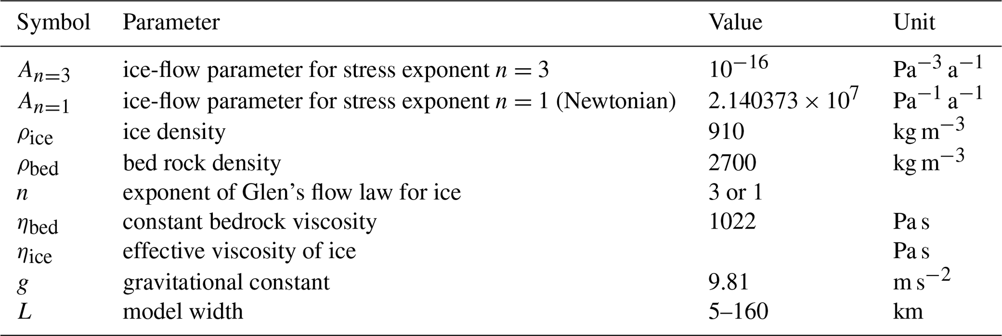
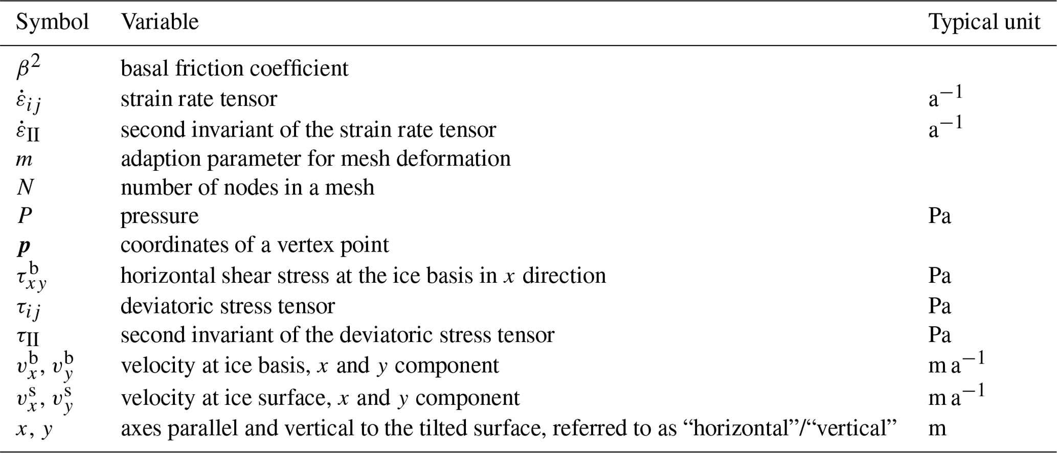
Here τij is the deviatoric stress tensor, P the pressure, g the gravitational acceleration and v the velocity (see Tables 1 and 2 for symbols used). Simulations are based on Glen's flow law for viscous flow (Glen, 1955), according to which the strain rate () is proportional to the deviatoric stress (τij) to the power n, the stress exponent. This flow law can be written as
where A is the temperature-dependent rate factor and τII the second invariant of the deviatoric stress tensor τij (Nye, 1953).
Based on Newtonian flow, where , we define an effective viscosity ηice after Eq. (3) as
Table 1Parameters and their values, as prescribed by Pattyn et al. (2008) for the intercomparison project.
2.2 Characteristics of Underworld with regard to specific challenges in the modeling of ice flow
Underworld is designed to solve some of the special problems relevant to modeling geodynamic processes. Identical problems arise in the modeling of ice. Some of these challenges are as follows:
-
the modeling of discontinuities in the material properties at layer boundaries, for instance, at the ice–rock and ice–air interfaces;
-
gradients within the ice, for instance, due to strain softening or thermal effects;
-
the tracking of the strain history;
-
the often extreme spatial extent of the modeled systems;
-
the very strong deformation of the material.
Underworld addresses these issues with the so-called material point method (MPM) (Sulsky et al., 1994; Moresi et al., 2003), which is closely related to the venerable particle-in-cell (PIC) method. MPM uses a Eulerian finite-element mesh in order to calculate the incremental development of the velocity field and other field variables, such as, temperature and pressure. In the MPM method, Lagrangian material points (“particles”) carry the density, viscosity, thermal conductivity and other relevant material parameters. They thereby record the history at their current location at every time step and some historical properties like the stress at previous time step for simulations of viscoelastic deformations (Farrington et al., 2014). The underlying mesh provides solutions for the incremental movement of the material points. The method is advantageous in the modeling of the emergence of structures (e.g., folding; see Mühlhaus et al., 2002) or where very strong deformation is involved, as in the deformation across shear zones or near the base of an ice sheet. In MPM, the mesh does not carry any history information other than deformation of the boundary and therefore can be re-meshed at any time as required and without loss of accuracy.
There is an unavoidable smoothing which comes from the coarseness of the computational mesh relative to the material point density (Moresi et al., 2003). While material boundaries are represented by a continuous interpolant on the grid, they are necessarily discrete in the case of particles. This can lead to fluctuations in the solution close to sharp rheological or mechanical boundaries (Yang et al., 2021), for instance, at the interface between ice and underlying rock. In the ice itself, a change in mechanical parameters is usually more gradual and is controlled, for example, by the temperature gradient.
Another complication in the numerical modeling of ice flow is the highly anisotropic behavior of ice, created by the near-orthotropic properties of the ice crystal. The possibility to model anisotropic flow is built into Underworld (Mühlhaus et al., 2004). Like any other local material property, the orientation of the anisotropy can be stored on the particle level.
Underworld offers a variety of possible solvers, including the well-known MUMPS, LU and multi-grid methods. We have carried out brief comparative precision tests with these solvers and could not find any difference in precision to the standard solver which is based on the multi-grid method. Throughout this study we will generally use MUMPS for 2D models and multi-grid for 3D models. The exception is tests of the computation time, for which we contrast a variety of solvers.
The ISMIP-HOM benchmark experiments have been described in detail in Pattyn and Payne (2006) and Pattyn et al. (2008). We perform all the experiments as described in these publications. For simplicity we also apply the same alphabetical numbering scheme and refer to the experiments as Experiment A to Experiment F. As we strive to focus on the essentials in the following descriptions, we refer to the original publications for further technical details if needed.
Experiments A, B, C and F are three-dimensional. Experiments D and E only consider two spatial dimensions, and Experiment B has an additional version in 2D. Experiments A through D are performed for a variety of horizontal system dimensions L, with L=5, 10, 20, 40, 80 or 160 km. Experiments A through E use a flow law based on n=3, and Experiment F applies Newtonian flow where n=1 (Table 1).
We tested the influence of the mesh geometry on the results and the CPU time consumption as a function of the total degree of freedom using Experiment D and the 2D version of Experiment B.
3.1 Experiments A and B
A and B consider a slab of ice with a mean ice thickness H=1000 m, lying on a sloping bed with a mean slope α=0.5∘. The bedrock topography consists of a series of sinusoidal bumps (Experiment A) or ripples (Experiment B) with an amplitude of 500 m (Fig. 1). The minimum thickness of the rock layer is 500 m, and the total height of the model is 2000 m. The flow of ice is governed by Eq. (3). The bedrock viscosity is constant, and ice is frozen to the bedrock. Relevant material parameters are compiled in Table 1.
The surface elevation is described by the formula
Bedrock topography for Experiment A is described using zs by
and for Experiment B by
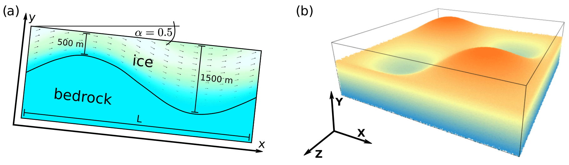
Figure 1(a) 2D geometry of Experiment B. This is identical to a section parallel X located at in Experiment A (right). Sloping angle α is given in degrees. Also depicted is the velocity field of the flowing ice, resulting for a model width L of 5000 m from the simulations described below. Color and arrow length visualize the amount of velocity. (b) Bedrock topography for Experiment A and general naming scheme for the axes of 3D experiments.
3.2 Experiments C and D
Experiments C and D are similar to Experiments A and B, although the topography of the bedrock is flat. Instead, the coefficient of basal friction β2 varies in a sinusoidal manner. The ice thickness H is constant at 1000 m. The slope angle α of the ice surface and of the underlying bedrock is 0.1∘. Ice flow is governed by Eq. (3), and the material parameters are summarized in Table 1. According to the benchmark specifications, Experiment C is run exclusively in 3D and Experiment D exclusively in 2D.
The basal friction coefficient relates the basal drag τb to the basal velocity vb by
With the coefficient of basal friction β2 for Experiment C is defined as
and for Experiment D by
Figure 2 shows the basal drag and the basal velocity calculated from Eq. (10) (Experiment D) and Eq. (8). Here, the velocity is calculated for a constant basal shear stress τb=ρicegHsin (α), according to the shallow-ice approximation (SIA) (Hutter, 1983). Notice the singularity in the velocity field (Fig. 2b), which develops because β2=0 at .
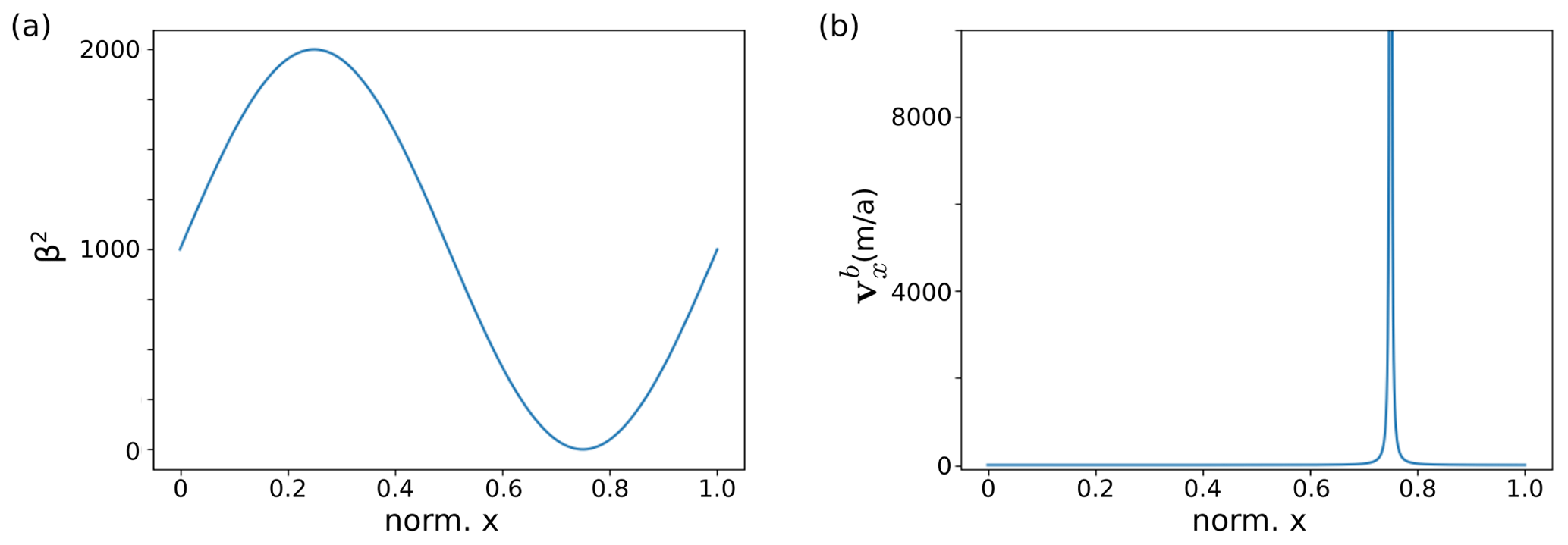
Figure 2(a) Basal drag β2 and (b) basal velocity plotted according to Eqs. (9) and (10) and applying the SIA, plotted for L=5000 m. Notice the singularity in the velocity field, which develops because β2=0 at , which is within the modeled domain.
3.3 Experiment E
Experiment E is a two-dimensional diagnostic experiment along the central flowline of a glacier in the European Alps (Haut Glacier d'Arolla). The basic experiment and geometry are described in Blatter et al. (1998) and by Pattyn et al. (2008). The general geometry of the glacier profile as used in the experiment is shown in Fig. 3. The experiment is run with two different basal conditions: (1) the ice is frozen to the ground everywhere (β2=∞), or (2) a zone of zero traction (β2=0) between x=2200 m and x=2500 m exists. Compare Eq. (8) for the meaning of the basal friction coefficient β2.
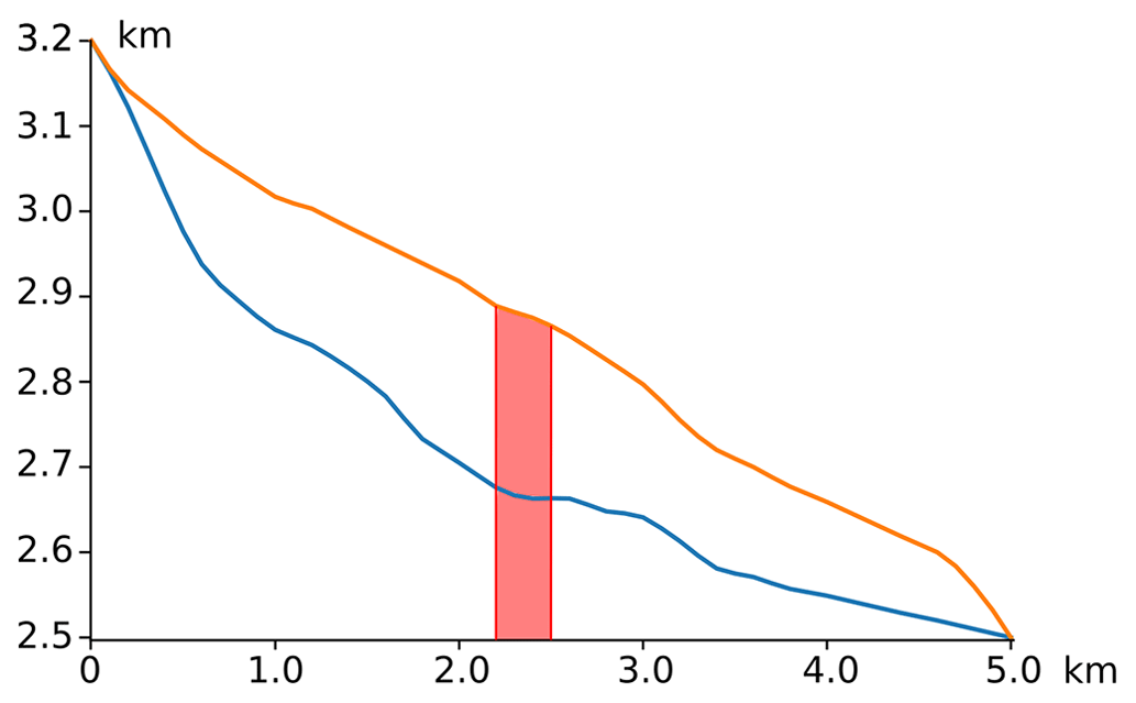
Figure 3Longitudinal profile of Haut Glacier d'Arolla (Pattyn et al., 2008). Blue line: contact ice–rock. Orange line: contact ice–air. Red zone: area of varying basal conditions, with either β2=∞ or β2=0.
3.4 Experiment F
Experiment F is a prognostic experiment in which a free ice surface relaxes until a steady state is reached for a zero surface mass balance. The slab of ice is resting on a bed with a mean slope α=3∘. The bedrock plane parallels the surface but is perturbed by a Gaussian bump. The initial bedrock (B0) and surface (S0) elevation are described by
where σ=10H0.
Experiment F applies a Newtonian (n=1) flow law, given in Table 1, so that the effective viscosity . The experiment is run with two different values for the slip ratio c, so that c=1 and c=0 is applied. c is used to describe the basal friction coefficient β2 (see Eq. 8) by
The model domain is discretized by quadrilateral Q1/P0 elements, where velocity is continuously linear, and pressure is discontinuously constant. The pressure grid is offset from the velocity grid. A direct comparison of the pressure at fixed locations to the results of other models is therefore prone to some interpolation error. Periodicity of the in- and outflow boundaries is applied in all experiments except Experiment E.
The ice–rock interface is defined by either of the two following methods, depending on the type of experiment: (i) by particles or (ii) directly by the mesh geometry.
4.1 FE grids with a rectangular hull
In most experiments we assume that the bedrock is identical to the basal grid boundary. In experiments with a flat bedrock topography (C, D and F), this means that the resulting shape of the mesh is rectangular.
An exception is the 2D version of Experiment B: in order to evaluate the impact of the mesh geometry and of a particle representation of the bedrock material, we define the sinusoidal bedrock topography using particles on a FE grid with a rectangular hull. Different materials are represented by particles with different rheological properties. Particles are assigned to either ice or bedrock depending on whether their depth exceeds the local ice thickness H. As pointed out, the material point method can lead to spurious fluctuations in gradients at material boundaries, if particles of different materials are both located in one element.
In order to test and improve this behavior, we define three different internal grid geometries and compare the smoothness of the resulting basal shear stress τb. These geometries are (i) a classic rectangular grid, (ii) a grid where the grid resolution increases in the vicinity of the ice–bedrock interface and (iii) a grid where the mesh perfectly fits the rock surface (Fig. 4).
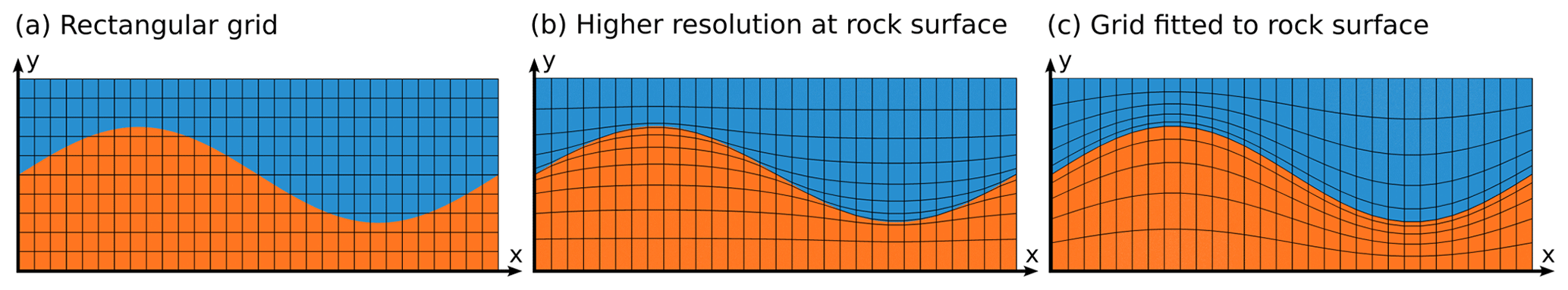
Figure 4(a) Rectangular mesh. (b) Structurally conforming mesh, with increased resolution at the ice–rock interface. (c) Mesh perfectly fits the rock surface. Blue: ice. Red: bedrock. For visualization purposes, both mesh resolution and distortion are reduced compared to the actual experiments. The structure parameter m=0.5 for both adapted grids (see Eqs. 14, 15). Mesh resolution: x=128, y=64. In the case of the rectangular mesh, it is additionally 256×128.
4.1.1 Rectangular grid geometry
The benchmark assumes a constant height of the model for each experiment, while the width is varied in a series of runs during such an experiment. It is typically expected that the accuracy of the solution and the computation time are most optimal if the aspect ratio of cells is close to 1.
4.1.2 Structurally conforming grid
We adapt the rectangular mesh to the underlying topography defined by the ice–rock boundary by vertically shifting its vertices, so that the model resolution is significantly increased close to the bedrock surface. Using the vertices of the regular rectangular grid as input, the new vertical y coordinate of a vertex point from the regular mesh becomes
We assume here that the grid in y direction originates at Y0=0 and ends in Y1=1. The rock surface is defined by a function s(x). is the vertical distance between the rock surface and p2. Both resolution and the geometry of individual cells are adapted to the interface line as shown in Fig. 3b. m is a structural adaption parameter, controlling the intensity of the mesh deformation. It is worth pointing out that the resolution in x is not affected by this geometry.
4.1.3 Grid fitted to ice–rock interface
The mesh defined by Eq. (14) does not guarantee that the ice–rock interface is aligned perfectly with finite-element edges. This may still introduce stress perturbations in elements containing different materials with strong viscosity contrasts (Yang et al., 2021). Therefore it makes sense to apply another mesh structure whose mesh edges fit the ice–rock interface exactly.
We define the new vertical y coordinate of a vertex point from the regular mesh by
The variable n denotes the nth node in the vertical y direction; n0 is a predefined node, which is relocated exactly to the rock surface; and nt is the total number of vertical vertexes. The difference between the equations above is that we fix n0 in Eq. (14), while n0 varies along the x direction for the case discussed in Eq. (15). As before, m is an adaption parameter which controls the intensity of the mesh deformation. The adaption of the grid geometry does not affect the position of nodes in the x direction.
4.2 FE grids with a non-rectangular hull
In all other experiments with an uneven bedrock topography (Experiments A and E and the 3D version of Experiment B) we apply Eq. (15) with m=0 to the lower system boundary. In the case of Experiment D, the ice–air interface is not flat; therefore particles represent ice and overlying air (Fig. 5).
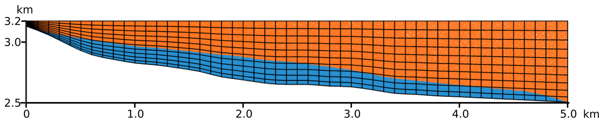
Figure 5Grid geometry and particle distribution used for Experiment E, representing Haut Glacier d'Arolla. Particles carry the rheological properties of ice and air. Blue: ice. Red: air.
4.3 Basal conditions
Underworld pre-implements no-slip and free-slip boundary conditions for flat system boundaries. However, Experiments C through E require the usage of a friction law. We realize the basal drag requirement by a basal layer with Newtonian viscosity, whose viscosity is dependent on the basal friction coefficient β2.
In the following, the relation between the Newtonian viscosity of this basal layer (ηb) and β2 is derived. For the sake of simplicity, we assume a flat horizontal surface, so that the usual notation can be used. In the case of an uneven base, x and y correspond to directions parallel or perpendicular to the lower system boundary.
Combining and integrating the relations (Newtonian flow) and (definition of the strain rate) leads to , with h the layer height. This relation is then used to define the local viscosity of the Newtonian layer. At the top of this layer, the velocity condition defined in Eq. (8) is satisfied.
Below, we will first examine the CPU time consumption as a function of the grid resolution and the effect of the grid geometry on the smoothness of results.
5.1 CPU time consumption
The mesh resolution is one of the most important parameters that controls the precision of the solution. Since computation time increases with resolution, it is desirable to establish a relationship between these two quantities. Below we test and display the CPU time of the initial solution of the 2D version of Experiment B. The computation time is not directly linked to the mesh resolution but instead to the degrees of freedom (DOF) of the system. For 2D-Stokes problems with quadrilateral elements, the degrees of freedom are 3N, with N the total number of nodes (Gagliardini and Zwinger, 2008). Figure 6 shows the relationship between the DOF and the computation time in a log–log plot for a series of 13 simulations with different resolutions and for different solvers (MUMPS, LU and multi-grid). The ratio of width to height of the grid cells remains constant in all experiments. On the hardware side, the simulations ran on a system with an Intel Xeon E5 processor with eight cores and 32 GB RAM. Of these eight cores, only one core was assigned to a trial run, and only one experiment was calculated at a time.
The interpolation between N and the computation time (s) expressed by a power regression is 0.00014N1.21 (multi-grid), 0.00037N1.06 (MUMPS) and 0.00013N1.15 (LU). In the case of the multi-grid method, outliers from the generally linear relation exist, which are related to the recursive refinement of the grid. Outliers do not exist for the direct solvers MUMPS and LU.
It is important to note, that – theoretically – the direct solvers should not scale better than N2. Therefore, the power regression cannot be used in order to extrapolate these results to an arbitrary DOF. It can be seen in Fig. 6 that a slight upward curvature of the data with regard to the interpolation exists.
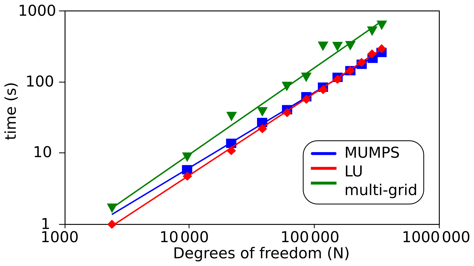
Figure 6Computation time for Experiment B plotted vs. the degrees of freedom and using different solvers. Blue: Mumps (0.00037N1.06). Red: LU (0.00013N1.15). Green: multi-grid (0.00014N1.212).
5.2 Impact of the grid geometry
We tested the impact of the grid geometry based on using the flow law parameters n=3 and Pa−3 a−1 (Pattyn et al., 2008). In order to increase effects related to the geometry, the mesh resolution is intentionally relatively small, at 128×64. Only for the rectangular grid is a larger resolution applied. The non-rectangular meshes use an adaption parameter m=0.25.
The results for the surface velocity are generally smooth and virtually identical in the three grid geometries. However, fluctuations of the shear stress can become considerable, especially close to the ice–bedrock interface (Fig. 7), depending on the type of FE grid. These fluctuations are largest if a low-resolution rectangular mesh is used. Increasing the resolution of the rectangular mesh does not fully eliminate the fluctuations but is a way to reduce the problem (as highlighted in Fig. 7c). A more conforming grid with an increased resolution around the rock surface (Eq. 1) reduces the fluctuations significantly but does not completely eliminate them (Fig. 7b). The unambiguously smoothest results are achieved using a grid fully fitted to the rock surface after Eq. (15) (see Fig. 7a). This confirms that fluctuations become smaller when there is less mixing of materials with different properties within an element.
The absence of fluctuations in the stress field is a measure for the ability of the model to deal with discontinuous material boundaries. In the following simulations for Experiment B, we will therefore exclusively apply the fitted mesh. This is in line with the original benchmark paper by Pattyn et al. (2008), who suggested testing the models with optimized settings.
The boundary between ice and the bedrock is usually the only nonplanar material boundary in glaciers and ice sheets. The other material boundary, between ice and air, can often be considered almost planar in the modeling of large ice sheets, while rheological changes within the ice itself can usually be treated as gradual, controlled, for instance, by the temperature field or the crystallographic fabric. It is an important conclusion from these results that a FE mesh fitted (even approximately) to the underlying bedrock topography can significantly improve the accuracy of ice flow simulations based on the material point method.
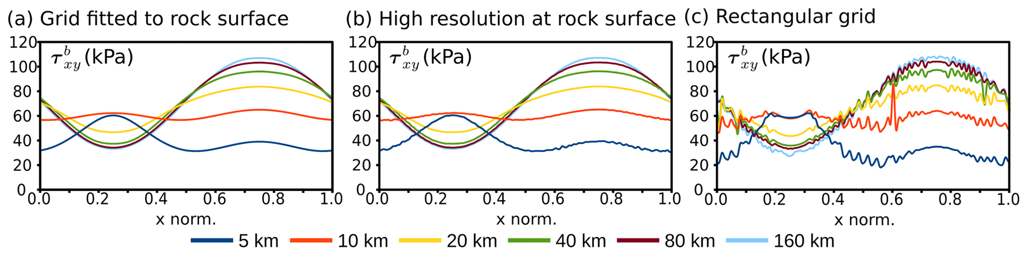
Figure 7The basal shear stress (in kPa), calculated on (a) a grid fitted to the rock surface, and (b) a structurally more conforming grid, which increases mesh resolution at the rock surface and (c) a rectangular grid. The experiments are based on a grid resolution of 128×64.
5.3 Impact of the grid resolution
Choosing a well-suited mesh resolution is always a balance between precision requirements and computational limitations. The computation limits can be related either to the hardware or to general time constraints, which do not allow for very long computation times. Also mesh geometry has an impact on the accuracy and may or may not require a larger resolution.
Given the existing time constraints and the number of simulations, this allowed us to test resolutions of 64×32 and 128×64 up to 256×128. Even at the relatively small resolution of 64×32, the solution for stress and velocity at the surface of the model is smooth and virtually identical to the results obtained with higher resolutions, independent of the mesh geometry (Sect. 5.2). This was different in the case of the interface between the ice and the underlying bedrock. While performance was good enough or very good with a resolution of 128×64 for grids adapted to the interface, a resolution of 256×128 was necessary to obtain usable results in the case of a rectangular mesh. Two grid points above the interface, the solution was smooth for all mesh geometries at 128×64 and did not differ from higher resolutions.
The highest-resolution 3D simulations ran mostly on a high-performance computer (HPC) cluster. Accuracy was systematically tested for Experiment B using a fitted grid, by comparing the results of the 2D and 3D experiments. Under perfect conditions, 2D and 3D simulations should yield identical results. We found that the necessary resolution is highly dependent on the system size, i.e., on the aspect ratio of the cells. For small system sizes of up to 20 km, we found that a minimum resolution of was necessary to produce similar results as for the 2D model. Larger systems already produced satisfactory results with a resolution of .
Below we will compare the results of the individual benchmark experiments generated by Underworld to the results of alternative codes. Where applicable, we run both the three-dimensional and the two-dimensional version of the benchmark experiments. This applies to Experiments B and C. For the latter, Experiment D is the associated 2D setup. All results are compiled in the Supplement to this paper. Concerning the output parameter Δp, which is the difference between the isotropic and the hydrostatic pressure, the curve progression is very similar to that of other full-Stokes models of the ISMIP but shows stronger fluctuations between adjacent evaluation points. This is due to the internal architecture of Underworld experiments, where the mesh used for the calculation of pressure is a sub-mesh of the velocity mesh with a staggered geometry. Fluctuations are a product of internal interpolation.
6.1 Experiments A and B
We fit the lower system boundary to the topography of the underlying bedrock in the 3D experiments by applying Eq. (15) with m=0.2 to the lower system boundary. The 2D version of Experiment B is based on a rectangular grid, which is internally fitted to the rock surface as in Sect. 5.2 above. Other relevant parameters are given in Table 1.
Results of Experiment A are shown in Figs. S1 and S2 in the Supplement and display the surface velocity and the basal shear stress. Results of Experiment B are shown in Fig. S3 to S6 in the Supplement and show surface velocity and basal shear stress in a 2D version of the experiment and at an arbitrary section paralleling the x axis of the 3D experiment. Diagrams include the results of full-Stokes solutions published in Pattyn et al. (2008) for comparison.
The surface velocity is controlled by the model width L and is in the range from a few meters per year to more than 100 m a−1. Figure 8 compares our results for Experiment B to results compiled from eight full-Stokes models that were previously published (Pattyn et al., 2008). A full comparison of the results is in the Supplement to this paper.
In Experiment B, the shape of the horizontal surface velocity for L=5 km differs significantly from that for the other cases. The surface velocity is larger over the bump and thus anti-correlated with the ice thickness. Gagliardini and Zwinger (2008) explain this as a mass conservation effect: horizontal flux cannot be balanced by vertical flux because the vertical velocity would be too large for the given system size. This phenomenon does not occur in Experiment A, with the same system size, although the section is identical at the chosen location. This can be explained because ice can flow around the sides of the bump.
Figure 8 shows the maximum and minimum surface velocity vx(ys) and the maximum basal shear stress τxy(yb) calculated by the 2D version of Experiment B and compares it to other full-Stokes solutions compiled by Pattyn et al. (2008). Maxima of both the shear stress and the surface velocity show a tendency to be at the lower end of the spectrum, while minima are virtually identical to the results from the comparison models. However, a full comparison (compare Supplement) shows a more diverse distribution of the results than the minima–maxima comparison in Fig. 6 implies. The results of our Experiments show generally a very good agreement with the majority of models, while some of the comparison models display large deviations with regard to the entire curve.
Figures S5 and S6 in the Supplement compare the results of the 2D and the 3D setup, which should be ideally identical. The results for the surface velocity are virtually identical, with exception of the L=5 km case, where a deviation of ∼2 % for the maximum and the minimum velocity exists if comparing 2D and 3D results. A similar effect exists regarding the extrema of the basal shear stress, which are most notable for L=5 km and L=10 km.
To shed some light on the difference between 2D and 3D results, we ran 3D simulations with a resolution of and of for these system sizes and compared them to the results of the 2D simulation (256×128). Regarding the surface velocity, the higher-resolution 3D mesh indeed yields results closer to the 2D result than the lower-resolution simulation (Fig. S6 in the Supplement). This is not the case for the basal shear stress, where the deviation from the 2D result is comparable for both resolutions.
Possible reasons are (a) different hardware, the 2D experiment, and the low-resolution 3D experiment running on the same machine while the high-resolution 3D experiment ran on a HPC cluster and (b) differences in the mesh geometry. The low-resolution simulations use an exponent m=0.25 in Eq. (15). For technical reasons m is set to 0 for experiments on the cluster.
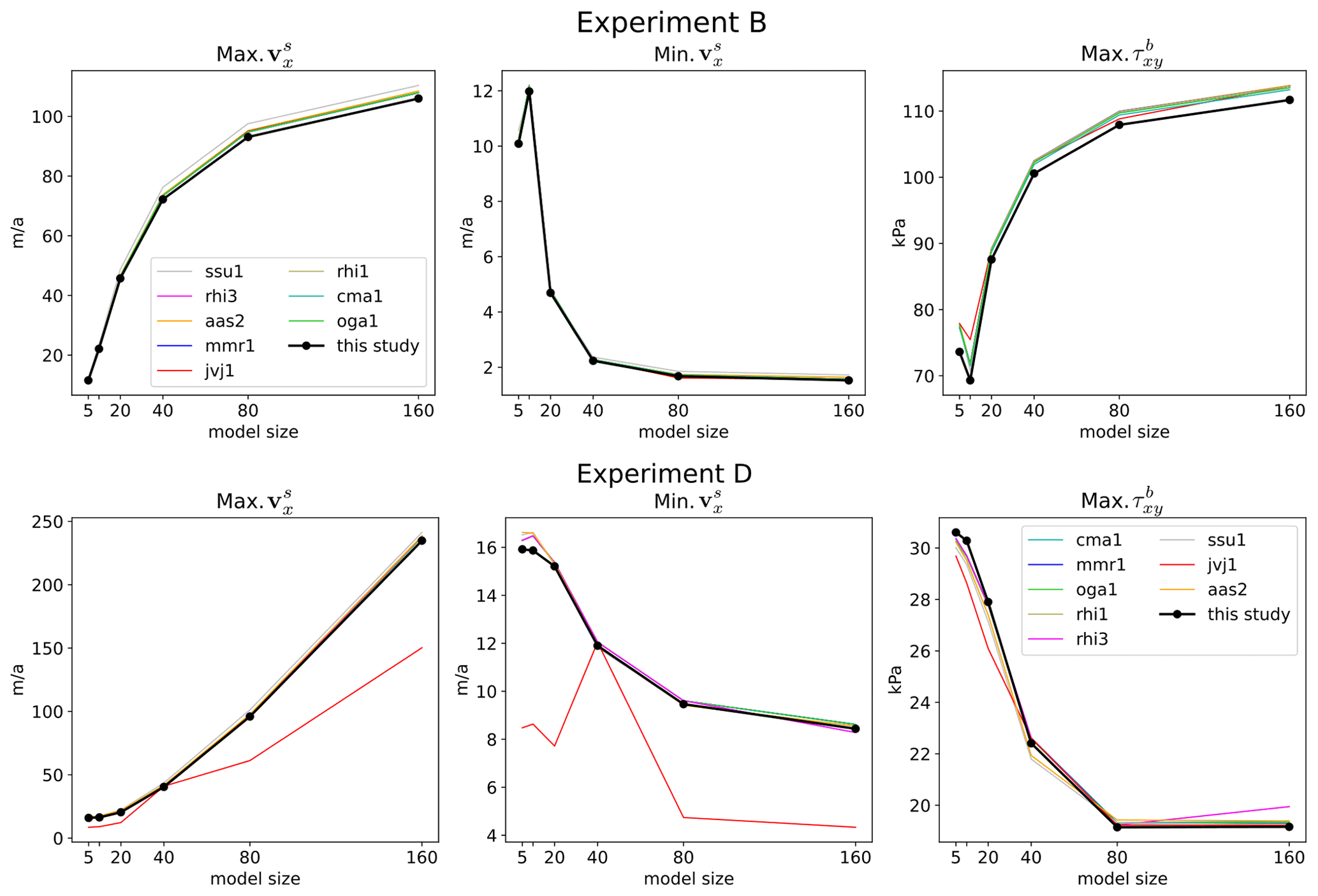
Figure 8Maximum and minimum values of the horizontal surface velocity (vx(ys)) and of the maximum basal shear stress (τxy(yb)) in Experiment B and D, plotted for every model size. The underlying FE mesh is fitted to the rock–ice interface. Results are compared to the results of eight full-Stokes models (compiled and published by Pattyn et al., 2008). Abbreviations of the comparison experiments are compiled in Table 3.
Table 3Model abbreviations used in the diagrams, taken from Pattyn et al., 2008. “Dimensions”: model dimensions. “Method”: numerical method: FE: finite element, Sp: spectral method, MPM: material point method.

6.2 Experiments C and D
Parameters for Experiments C and D are given in Table 1 for n=3. Results are summarized in Figs. S6 and S7 (Experiment C) and Figs. S8 and S9 (Experiment D) in the Supplement.
In Experiment C, the surface velocity is strongly dependent on the system size L. In the case of the smallest system size (L=5 km), the surface velocity is close to constant at ∼16 m a−1. With L=160 km it ranges from 8.8 up to 122.5 m a−1 (Fig. S7, Supplement). The shear stress results of the Underworld simulations line up well with the comparison simulations. They show a sinusoidal curve with a maximum at and a minimum at . With increasing model size, the maximum gets progressively flattened. The peak downwards at the singularity value is far less impacted by model size, which means it gets more dominant for bigger values of L.
In Experiment D, the maximum surface velocity increases with model width L and is in the range from 16 m a−1 to more than 235 m a−1. Figure 9 shows the maximum and minimum surface velocity and the maximum shear stress τxy. Results are generally in good agreement with the majority of model results they are compared to. However, the general variation between the results of the comparison models is generally larger than in the 2D version of Experiment B, the only other 2D experiment of the benchmark. The same statement applies to basal shear stress. Again, a full comparison of the results is included in the Supplement to this paper.
6.3 Experiments E and F
Experiment E is calculated for two different setups, where either the entire glacier is frozen to the underlying bedrock or where a traction-free section close to the center exists. In both cases, the results of Underworld lie within the range of the comparison models (see Figs. S10 and S11 in the Supplement). Both the calculated surface velocity and the basal shear stress are in the lower range of this range, which is true for the majority of models. In particular, extreme values of the curve are a bit smoother than in some of the other full-Stokes models.
The prognostic Experiment F calculates the surface velocity and the surface topography. Results are compiled in Figs. S12 and S13 in the Supplement. Since the majority of potential comparison models are not capable of calculating a free surface, the results of Underworld can be compared to only two other software packages. Due to the special properties of the software, we only model the version of the experiment with a basal no-slip condition. Other values for the basal traction would either involve a very complex implementation or yield questionable results. We ran the model until no further change in topography or velocity occurred and interpreted this as the stable state.
When we compare our results with those of the two reference models with respect to an analytical sample solution (Frank Pattyn, personal communication, 2022), qualitatively similar results are obtained. One of the reference models shows very good agreement with the theoretical surface elevation but shows lower accuracy with respect to surface velocity. Underworld predicts the surface velocity the best of the three models but tends to develop a slightly less extreme topography than the analytical solution.
Ice is assumed to deform mostly by dislocation creep at natural strain rates (Budd and Jacka, 1989), whereby slip along the basal planes is much easier than slip along the other slip planes (Duval et al., 1983). This makes an ice single crystal mechanically effectively transversely isotropic, with the c axis that is oriented perpendicular to the basal plane as the symmetry axis. The anisotropy of ice single crystals leads to a crystallographic preferred orientation (CPO) in a deforming aggregate of ice crystals (Alley, 1988; Llorens et al., 2017). The mechanical anisotropy of an aggregate may be of a lower symmetry than that of a single crystal but can be approximated to a first order as orthotropic (Gillet-Chaulet et al., 2006).
One of the features of Underworld which makes it interesting for the modeling of ice is its capability to model linear orthotropic viscosity, which includes transverse isotropy as a special case. In order to demonstrate its effect, we set up comparison experiments with anisotropic and isotropic ice rheology, based on the setup of Experiment B: ice flows over a sinusoidal surface, driven by a general 0.5∘ tilt of the model. Isotropic flow is governed by Eq. (4), using the parameters given in Table 1.
The orientation of the anisotropy is stored as the c axis orientation on the level of the particles in Underworld. The aggregate anisotropy of one mesh element is calculated from the individual c axis orientations of the cloud of particles in an element. Fabric evolution is simulated using the rotation of the c axes in the flow field after, e.g., Gillet-Chaulet et al. (2006) or Richards et al. (2021). However, for simplicity, in our example here we assume that all basal planes are and remain horizontal. The anisotropy of ice, in terms of the ratio of resistance to slip parallel to crystallographic non-basal and basal planes, is about 60–80 in a single ice crystal (Duval et al., 1983). However, as we simulate aggregates of crystals here, we set the viscosity for shear non-parallel to the basal planes only 10 times higher than the viscosity for shear parallel to the basal planes, which we assume equal to that used for the isotropic flow law.
Figure 9 shows the shape of marker lines prior to deformation and after 750 years of flow for both iso- and anisotropic ice models. Marker lines inherit their sinusoidal shape from the shape of the underlying topography and are then folded according to the localization of the highest shear rates. In isotropic ice (Fig. 9b), the axial plane of the shear fold is mostly controlled by the underlying topography. In the case of anisotropic ice (Fig. 9c), the folding is more intense, and the axial plane is subhorizontal, showing that the anisotropy has a distinct effect on resulting fold structures.
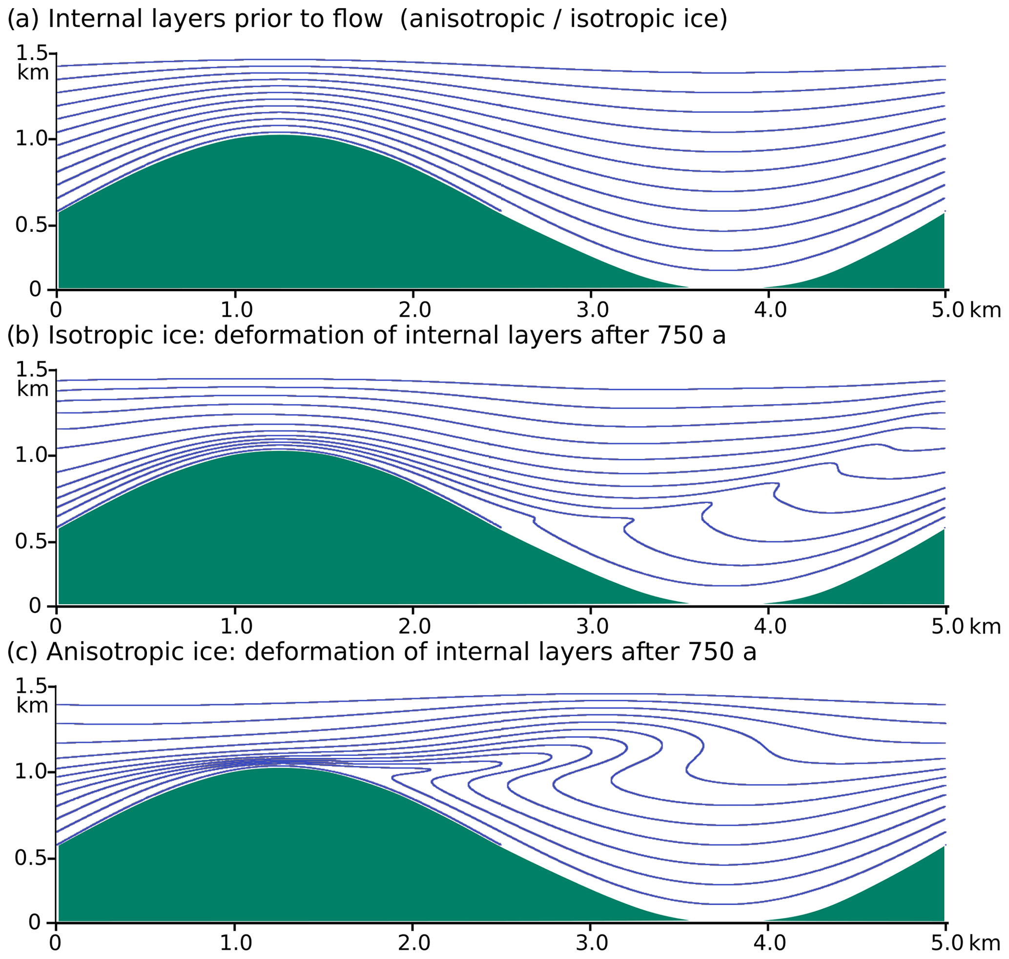
Figure 9Marker lines prior to (a) and after 750 years of flow of (b) isotropic and (c) anisotropic ice. The axial plane of the resulting shear fold in isotropic ice mimics the bedrock topography, while it is controlled by shearing along a horizontal shear zone in the case of anisotropic ice. Green: bedrock, flow to the right.
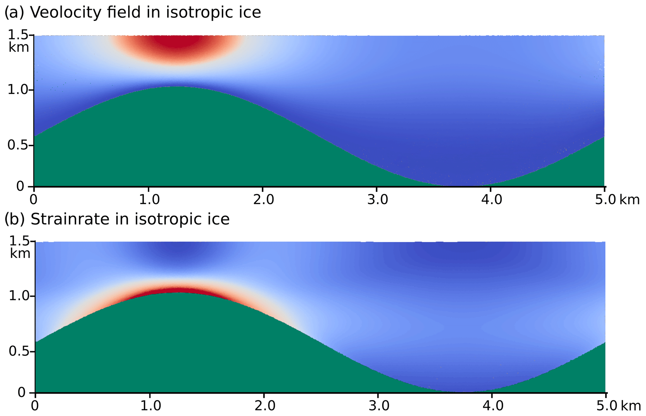
Figure 10Velocity field and strain rate field in isotropic ice. Large strain rates and velocities occur in the vicinity of the bottleneck formed by the crest of the hill. Green: bedrock. For velocity, red is 70 m a−1 and blue is 0 m a−1. For strain rate, red is 0.032 a−1, and blue is 0 a−1.
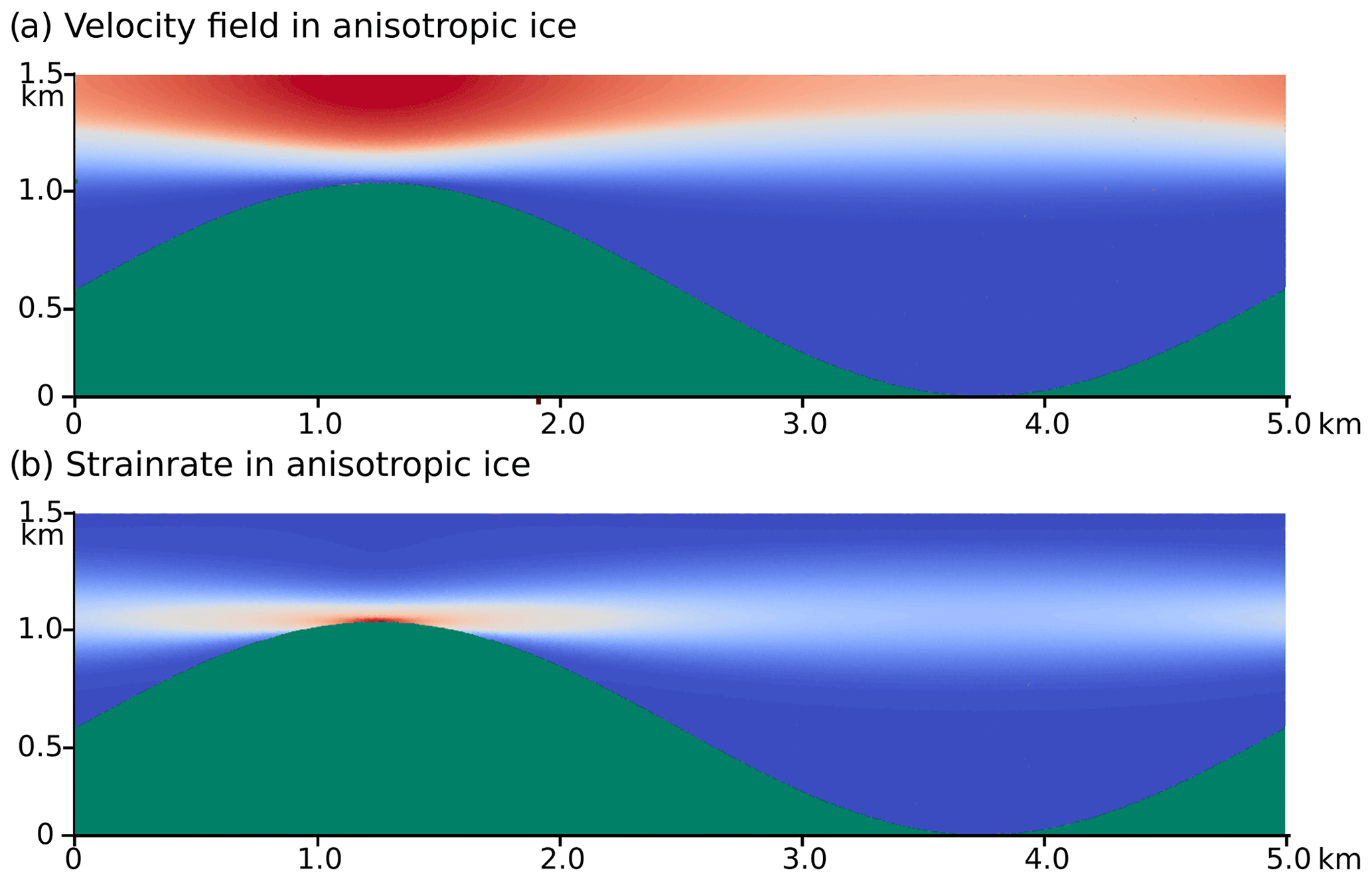
Figure 11Velocity field and strain rate field in anisotropic ice. The velocity field is vertically subdivided into a fast-flowing upper and an almost stagnant lower part. The strain rate is thus at its maximum in the horizontal shear zone that spans from crest to crest of the bedrock undulations. Green: bedrock, velocity: red: 6.6 m a−1, blue: 0 m a−1, strain rate: red: 0.031 a−1, blue: 0 a−1.
Figures 10 and 11 that show the velocity field and the strain rate field in both materials allow for a better understanding of the deformation process. In the case of isotropic ice, the flow field is controlled by the underlying topography. Hence the hill on the left acts as a bottleneck for the ice flow, and the hill sides funnel ice in and out of the bottleneck region. Consequently, the zone of high shear strain at the ice–rock interface extends across the crest of the bedrock bump (Fig. 10a) and the maximum velocity above it. Outside the bottleneck region, flow is comparatively evenly distributed.
In the case of anisotropic ice, the flow regime and thus the shear folding is quite different. Here, flow is strongly controlled by the inherent anisotropy and far less by the bedrock topography. Looking at the velocity field (Fig. 11a), it becomes clear that the flow field is internally subdivided into a fast-flowing upper part and slow-flowing “dead ice” in the lower part. Decoupling of the shallow and deep ice develops because the anisotropy facilitates shear along the horizontal basal planes. The resulting horizontal high-strain zone spans the entire system and produces the distinct shear fold.
One of the great advantages of the Underword2 software package from the standpoint of the modeler is its great flexibility and traceability due to its hybrid nature as both a particle and a finite-element model. Another contribution to its flexibility is the easy extensibility of the core code and the interactive development thanks to the existence of a Python API. The compatibility of the API with the mathematical–scientific packages NumPy and SciPy provides easy access to a wide range of numerical resources. Anisotropic flow and heat flow are already part of the core package.
Given the current debates in the ice community about the role of the anisotropy and hence of the fabric evolution of ice or the ideas for improvements of the flow laws for ice (e.g., Kennedy et al., 2013; Llorens et al., 2017; Richards et al., 2021; Martín et al., 2009), this type of flexibility is an important precondition for a future proof numerical model for glacier ice. One example was the implementation of the orthotropic rheology and the fabric evolution in deformed ice following Gödert (2003) and Gillet-Chaulet et al. (2006) by the authors of this text. Possible improvements to the fabric evolution models – for instance, by the SpecCAF model (Richards et al., 2021) – can be easily implemented and tested.
A few desirable features are currently still missing but are on the road map for future versions of Underworld. The soon-to-be-released Underworld3, for instance, allows for greater flexibility of the mesh geometry, including the triangulation of shapes and areas with arbitrary geometry.
The Underworld software is designed to solve deformation in complex geodynamic systems with nonlinear elastic–viscous–plastic materials, for which it provides a full-Stokes solution. It is therefore well suited for the modeling of glacier and ice-sheet flow, as it includes heat flow and anisotropic rheology. The combination of Lagrangian mass points (particles) and a Eulerian finite-element solution allows for the tracking of individual points as well as of inner and outer surfaces, such as deforming stratigraphic layers, but also of the thermal–mechanical properties in deforming materials. In the case of large rheological differences across interfaces, the possibility to fit the grid to the interface greatly improves the accuracy of stress field, compared to other grid types. In the case of ice flow experiments, it makes sense to fit the grid to the bedrock–ice boundary.
We compared results of Underworld simulations with those of other modeling approaches for the set of benchmark experiments provided by Pattyn et al. (2008). Our results match the full-Stokes solutions that are compiled in that study. This means that Underworld is a viable alternative to other full-Stokes models, in particular where the material point method is advantageous, such as when accurate tracking of material volumes or stratigraphic layers is desired. A further advantage is that, owing to the built-in Python API, Underworld is very flexible and can be extended to be applied to even the more complex processes which are involved in the flow of ice sheets and glaciers.
The program code that defines the experiments discussed in this article is included in the Supplement to this article, along with graphical representations and text files of the results. They are also available through Yang and Giordani (2022; https://doi.org/10.5281/zenodo.7384424). Underworld is fully open-source. The version (v2.12.0b) used for this paper is available through Mansour et al. (2022; https://doi.org/10.5281/zenodo.5935717). The most recent version is available through Beucher et al. (2022b; https://doi.org/10.5281/zenodo.6820562).
The supplement related to this article is available online at: https://doi.org/10.5194/gmd-15-8749-2022-supplement.
TS and PB discussed and designed the first implementation of the benchmark experiments. HY provided the code and the concept behind the applied mesh geometries. TS and HY developed and tested the code and performed some simulations. JL performed most of the 3D experiments and compiled the related data files and data plots. TS performed the 2D simulations and compiled the related data files and data plots. TS prepared the manuscript with many contributions, corrections and revisions from all authors. PB and LM provided important guidance.
The contact author has declared that none of the authors has any competing interests.
Publisher's note: Copernicus Publications remains neutral with regard to jurisdictional claims in published maps and institutional affiliations.
This open-access publication was funded by the University of Tübingen.
This paper was edited by Mauro Cacace and reviewed by Frank Pattyn and one anonymous referee.
Alley, R. B.: Fabrics in polar ice sheets: development and prediction, Science, 240, 493–495, 1988
Azuma, N.: A flow law for anisotropic ice and its application to ice sheets, Earth Planet. Sc. Lett., 128, 601–614, https://doi.org/10.1016/0012-821X(94)90173-2, 1994.
Bahadori, A., Holt. W. E., Feng, R., Austermann, J., Loughney, K. M., Salles, T., Moresi, L., Beucher, R., Lu, N., Flesch, L. M., Calvelage, C. M., Rasbury, E. T. Davis, D. M., Potochnik, A. R., Ward, W. B., Hatton, K., Haq, S. S. B., Smiley T. M., Wooton, K. M., and Badgley, C.: Coupled influence of tectonics, climate, and surface processes on landscape evolution in southwestern North America, Nat. Commun., 13, 4437, https://doi.org/10.1038/s41467-022-31903-2, 2022.
Beucher, R., Giordani, J., Moresi, L., Mansour, J., Kaluza, O., Velic, M., Farrington, R., Quenette, S., Beall, A., Sandiford, D., Mondy, L., Mallard, C., Rey, P., Duclaux, G., Laik, A., Morón, S., Beall, A., Knight, B., and Lu, N.: Underworld2: Python Geodynamics Modelling for Desktop, HPC and Cloud (v2.13.0b), Zenodo [code], https://doi.org/10.5281/zenodo.6820562, 2022a.
Beucher, R., Giordani, J., Moresi, L., Mansour, J., Kaluza, O., Velic, M., Farrington, R., Quenette, S., Beall, A., Sandiford, D., Mondy, L., Mallard, C., Rey, P., Duclaux, G., Laik, A., Morón, S., Beall, A., Knight, B., and Lu, N.: Underworld2: Python Geodynamics Modelling for Desktop, HPC and Cloud (v2.13.0b), Zenodo [code], https://doi.org/10.5281/zenodo.6820562, 2022b.
Blatter, H., Clarke, G., and Colinge, J.: Stress and velocity fields inglaciers: Part II.sliding and basal stress distribution, J. Glaciol., 44, 457–466, 1998.
Bons, P. D., Jansen, D., Mundel, F., Bauer, C. C., Binder, T., Eisen, O., Jessell, M.-G., Llorens, M., Steinbach, F., Steinhage, D., and Weikusat, I.: Converging flow and anisotropy cause large-scale folding in Greenland's ice sheet, Nat. Commun., 7, 11427, https://doi.org/10.1038/ncomms11427, 2016.
Bons, P. D., Kleiner, T., Llorens, M.-G., Prior, D. J., Sachau, T., Weikusat, I., and Jansen, D.: Greenland Ice Sheet: Higher nonlinearity of ice flow significantly reduces estimated basal motion, Geophys. Res. Lett., 45, 6542–6548, https://doi.org/10.1029/2018GL078356, 2018.
Bons, P. D., de Riese, T., Franke, S., Llorens, M.-G., Sachau, T., Stoll, N., Weikusat, I., Westhoff, J., and Zhang, Y.: Comment on “Exceptionally high heat flux needed to sustain the Northeast Greenland Ice Stream” by Smith-Johnsen et al. (2020), The Cryosphere, 15, 2251–2254, https://doi.org/10.5194/tc-15-2251-2021, 2021.
Budd, W. and Jacka, T.: A review of ice rheology for ice sheet modelling, Cold Reg. Sci. Technol., 16, 107–144, 1989.
Capitanio, F. A., Nebel, O., Cawood, P. A., Weinberg, R. F., and Clos, F.: Lithosphere differentiation in the early Earth controls Archean tectonics, Earth Planet. Sc. Lett., 525, 115755, https://doi.org/10.1016/j.epsl.2019.115755, 2019.
Carluccio, R., Kaus, B., Capitanio, F. A., and Moresi, L. N.: The Impact of a Very Weak and Thin Upper Asthenosphere on Subduction Motions, Geophys. Res. Lett., 46, 11893–11905, https://doi.org/10.1029/2019GL085212, 2019.
Cavitte, M. G. P., Blankenship, D. D., Young, D. A., Schroeder, D. M., Parrenin, F., Lemeur, E., Macgregor, J. A., and Siegert, M. J.: Deep radiostratigraphy of the East Antarctic plateau: connecting the Dome C and Vostok ice core sites, J. Glaciol., 62, 323–334, https://doi.org/10.1017/jog.2016.11, 2016.
Duval, P., Ashby, M. F., and Anderman, I.: Rate-controlling processes in the creep of polycrystalline ice, J. Phys. Chem., 87, 4066–4074, https://doi.org/10.1021/j100244a014, 1983.
Ershadi, M. R., Drews, R., Martín, C., Eisen, O., Ritz, C., Corr, H., Christmann, J., Zeising, O., Humbert, A., and Mulvaney, R.: Polarimetric radar reveals the spatial distribution of ice fabric at domes and divides in East Antarctica, The Cryosphere, 16, 1719–1739, https://doi.org/10.5194/tc-16-1719-2022, 2022.
Evans, B. and Kohlstedt, D. L.: Rheology of Rocks, in: Rock Physics and Phase Relations: a handbook of Physical Constants, Ref. Shelf, vol. 3, edited by: Ahrens, T. J., 148–165, AGU, Washington D.C., 1995.
Farrington, R. J., Moresi, L. N., and Capitanio, F. A.: The role of viscoelasticity in subducting plates, Geochem. Geophys. Geosyst., 15, 4291–4304, 2014.
Gagliardini, O. and Zwinger, T.: The ISMIP-HOM benchmark experiments performed using the Finite-Element code Elmer, The Cryosphere, 2, 67–76, https://doi.org/10.5194/tc-2-67-2008, 2008.
Gagliardini, O., Zwinger, T., Gillet-Chaulet, F., Durand, G., Favier, L., de Fleurian, B., Greve, R., Malinen, M., Martín, C., Råback, P., Ruokolainen, J., Sacchettini, M., Schäfer, M., Seddik, H., and Thies, J.: Capabilities and performance of Elmer/Ice, a new-generation ice sheet model, Geosci. Model Dev., 6, 1299–1318, https://doi.org/10.5194/gmd-6-1299-2013, 2013.
Gillet-Chaulet, f., Gagliardini, O., Meyssonnier, J., Zwinger, T., and Ruokolainen, J.: Flow-induced anisotropy in polar ice and related ice-sheet flow modelling, J. Non-Newtonian Fluid Mech., 134, 33–43, 2006.
Glen, J. W.: The Creep of Polycrystalline Ice, P. Roy. Soc. A, 228, 519–538, https://doi.org/10.1098/rspa.1955.0066, 1955.
Gödert, G.: A Mesoscopic Approach for Modelling Texture Evolution of Polar Ice Including Recrystallization Phenomena, Ann. Glaciol., 37, 23–28, https://doi.org/10.3189/172756403781815375, 2003.
Goelzer, H., Robinson, A., Seroussi, H., and van de Wal, R. S. W.: Recent progress in Greenland Ice Sheet modelling, Current Climate Change Reports, 3, 291–302, https://doi.org/10.1007/s40641-017-0073-y, 2017.
Goldsby, D. L.: Superplastic flow of ice relevant to glacier and ice-sheet mechanics, in: Glacier Science and Environmental Change, edited by: Knight, P. G., Blackwell, Oxford, 308–314, https://doi.org/10.1002/9780470750636.ch60, 2006.
Goldsby, D. L. and Kohlstedt, D. L.: Superplastic deformation of ice: Experimental observations, J. Geophys. Res., 106, 11017–11030, https://doi.org/10.1029/2000JB900336, 2001.
Haefeli, R.: Contribution to the movement and the form of ice sheets in the Arctic and Antarctic, J. Glaciol., 3, 1133–1151, 1961.
Hindmarsh, R. C. A.: A numerical comparison of approximations to the Stokes equations used in ice sheet and glacier modeling: HIGHER-ORDER GLACIER MODELS, J. Geophys. Res.-Earth Surf., 109, F1, https://doi.org/10.1029/2003JF000065, 2004.
Hutter, K. (Ed.): Theoretical glaciology: material science of ice and the mechanics of glaciers and ice sheets, D. Reidel Publishing Co., Dordrecht, 1983.
Jacobson, H. P. and Raymond, C. E. Thermal effects on the location of ice stream margins, J. Geophys. Res., 103, 12111–12122, 1998.
Johnson, J. V. and Staiger, J. W.: Modeling long-term stability of the Ferrar Glacier, East Antarctica: Implications for interpreting cosmogenic nuclide inheritance, J. Geophys. Res., 112, F03S30, https://doi.org/10.1029/2006JF000599, 2007.
Kennedy, J. H., Pettit, E. C., and Di Prinzio, C. L.: The evolution of crystal fabric in ice sheets and its link to climate history, J. Glaciol., 59, 357–373, https://doi.org/10.3189/2013JoG12J159, 2013.
Korchinski, M., Rey, P. F., Mondy, L., Teyssier, C., and Whitney, D. L.: Numerical investigation of deep-crust behavior under lithospheric extension, Tectonophysics, 726, 137–146. https://doi.org/10.1016/j.tecto.2017.12.029, 2018.
Leysinger-Vieli, G. J.-M. C., Martín, C., Hindmarsh, R. C. A., and Lüthi, M. P.: Basal freeze-on generates complex ice-sheet stratigraphy, Nat. Commun., 9, 4669, https://doi.org/10.1038/s41467-018-07083-3, 2018.
Llorens, M.-G., Griera, A., Steinbach, F., Bons, P. D., Gomez-Rivas, E., Jansen, D., Roessiger, J., Lebensohn, R. A., and Weikusat, I.: Dynamic recrystallization during deformation of polycrystalline ice: insights from numerical simulations, Philos. T. R. Soc. Math. Phys. Eng. Sci., 375, 20150346, https://doi.org/10.1098/rsta.2015.0346, 2017.
MacGregor, J. A., Fahnestock, M. A., Catania, G. A., Paden, J. D., Prasad Gogineni, S., Young, S. K., Rybarski, S. C., Mabrey, A. N., Wagman, B. M., and Morlighem, M.: Radiostratigraphy and age structure of the Greenland Ice Sheet, J. Geophys. Res.-Earth Surf., 120, 212–241, https://doi.org/10.1002/2014JF003215, 2015.
Mansour, J., Giordani, J., Moresi, L., Beucher, R., Kaluza, O., Velic, M., Farrington, R., Quenette, S., and Beall, A.: Underworld2: Python Geodynamics Modelling for Desktop, HPC and Cloud, JOSS, 5, 1797, https://doi.org/10.21105/joss.01797, 2020.
Mansour, J., Giordani, J., Moresi, L., Beucher, R., Kaluza, O., Velic, M., Farrington, R., Quenette, S., and Beall, A.: Underworld2: Python Geodynamics Modelling for Desktop, HPC and Cloud (v2.12.0b), Zenodo [code], https://doi.org/10.5281/zenodo.5935717, 2022.
Martín, C., Navarro, F., Otero, J., Cuadrado, M. L., and Corcuera, M. I.: Three-dimensional modelling of the dynamics of Johnsons Glacier, Livingston Island, Antarctica, Ann. Glaciol., 39, 1–8, https://doi.org/10.3189/172756404781814537, 2004.
Martín, C., Gudmundsson, G. H., Pritchard, H. D., and Gagliardini, O.: On the effects of anisotropic rheology on ice flow, internal structure, and the age-depth relationship at ice divides, J. Geophys. Res., 114, F04001, https://doi.org/10.1029/2008JF001204, 2009.
Mather, B., Müller, R.D., O'Neill, C., Beall, A., Vervoort, R. W., and Moresi, L.: Constraining the response of continental-scale groundwater flow to climate change, Sci. Rep.-UK, 12, 1–16, 2022.
McConnell, J. C. and Kidd, D. A.: On the plasticity of glacier and other ice, P. Roy. Soc. London, 44, 331–367, 1888.
Moresi, L. and Mühlhaus, H. B.: Anisotropic viscous models of large-deformation Mohr–Coulomb failure, Philosophical Magazine, 86, 3287–3305, 2006.
Moresi, L., Dufour, F., and Mühlhaus, H.-B.: A Lagrangian integration point finite element method for large deformation modeling of viscoelastic geomaterials, J. Comput. Phys., 184, 476–497, https://doi.org/10.1016/S0021-9991(02)00031-1, 2003.
Moresi, L., Quenette, S., Lemiale, V., Meriaux, C., and Appelbe, B.: Computational approaches to studying non-linear dynamics of the crust and mantle, Phy. Earth Planet. Int., 15, 69–82, 2007.
Mühlhaus, H.-B., Moresi, L., Hobbs, B., and Dufour, F. D. R.: Large Amplitude Folding in Finely Layered Viscoelastic Rock Structures, Pure Appl. Geophys., 159, 23, https://doi.org/10.1007/s00024-002-8737-4, 2002.
Mühlhaus, H.-B., Moresi, L., and Cada, M.: Emergent Anisotropy and Flow Alignment in Viscous Rock, Pure Appl. Geophys., 161, 2451–2463, https://doi.org/10.1007/s00024-004-2575-5, 2004.
NEEM community members: Eemian interglacial reconstructed from a Greenland folded ice core, Nature, 493, 489–494, https://doi.org/10.1038/nature11789, 2013.
Nye, J. F.: The Flow Law of Ice from Measurements in Glacier Tunnels, Laboratory Experiments and the Jungfraufirn Borehole Experiment, P. Roy. Soc. A, 219, 477–489, https://doi.org/10.1098/rspa.1953.0161, 1953.
Pattyn, F. and Payne, T.: Benchmark experiments for numerical Higher-Order ice-sheet Models, https://frank.pattyn.web.ulb.be/ismip/welcome.html (last access: 30 May 2022), 2006.
Pattyn, F., Perichon, L., Aschwanden, A., Breuer, B., de Smedt, B., Gagliardini, O., Gudmundsson, G. H., Hindmarsh, R. C. A., Hubbard, A., Johnson, J. V., Kleiner, T., Konovalov, Y., Martin, C., Payne, A. J., Pollard, D., Price, S., Rückamp, M., Saito, F., Souček, O., Sugiyama, S., and Zwinger, T.: Benchmark experiments for higher-order and full-Stokes ice sheet models (ISMIP–HOM), The Cryosphere, 2, 95–108, https://doi.org/10.5194/tc-2-95-2008, 2008.
Ranalli, G.: Rheology of the Earth., 366 pp., Allen and Unwin, Concord, Mass., 1987.
Ranganathan, M., Minchew, B., Meyer, C. R., and Peč, M.: Recrystallization of ice enhances the creep and vulnerability to fracture of ice shelves, Earth Planet. Sc. Lett., 576, 11721, https://doi.org/10.1016/j.epsl.2021.117219, 2021.
Rathmann, N. M. and Lilien, D. A.: Inferred basal friction and mass flux affected by crystal-orientation fabrics, J. Glaciol., 68, 236–252, https://doi.org/10.1017/jog.2021.88, 2022.
Richards, D. H. M., Pegler, S. S., Piazolo, S., and Harlen, O. G.: The evolution of ice fabrics: A continuum modelling approach validated against laboratory experiments, Earth Planet. Sci. Lett., 556, 116718, https://doi.org/10.1016/j.epsl.2020.116718, 2021.
Salles, T., Ding, X., and Brocard, G.: pyBadlands: A framework to simulate sediment transport, landscape dynamics and basin stratigraphic evolution through space and time, edited by: Borazjani, I., PLoS ONE, 13, e0195557, https://doi.org/10.1371/journal.pone.0195557, 2018.
Sandiford, D., Moresi, L. M., Sandiford, M., Farrington, R., and Yang, T.: The Fingerprints of Flexure in Slab Seismicity, Tectonics, 39, e2019TC005894, https://doi.org/10.1029/2019TC005894, 2020.
Schroeder, D. M., Bingham, R. G., Blankenship, D. D., Christianson, K., Eisen, O., Flowers, G. E., Karlsson, N. B., Koutnik, M. R., Paden, J. D., and Siegert, M. J.: Five decades of radioglaciology, Ann. Glaciol., 61, 1–13, 2020.
Sharples, W., Moresi, L. N., Velic, M., Jadamec, M. A., and May, D. A.: Simulating faults and plate boundaries with a transversely isotropic plasticity model, Phys. Earth Planet. Int., 252, 77–90, 2016.
Smith-Johnsen, S., Schlegel, N.-J., Fleurian, B., and Nisancioglu, K. H.: Sensitivity of the Northeast Greenland Ice Stream to Geothermal Heat, J. Geophys. Res.-Earth Surf., 125, e2019JF005252, https://doi.org/10.1029/2019JF005252, 2020.
Sugiyama, S., Gudmundsson, G. H., and Helbing, J.: Numerical investigation of the effects of temporal variations in basal lubrication on englacial strain-rate distribution, Ann. Glaciol., 37, 49–54, https://doi.org/10.3189/172756403781815618, 2003.
Sulsky, D., Chen, Z. and Schreyer, H. L.: A particle method for history-dependent materials, Comput. Meth. Appl. Mech. Eng., 118, 179–196, https://doi.org/10.1016/0045-7825(94)90112-0, 1994.
Wolovick, M. J., Creyts, T. T., Buck, W. R., and Bell, R. E.: Traveling slippery patches produce thickness-scale folds in ice sheets: Traveling slippery patches, Geophys. Res. Lett., 41, 8895–8901, https://doi.org/10.1002/2014GL062248, 2014.
Yang, H. and Giordani, J.: underworld-community/sachau-et-al-ice-sheet: v1.1 (v1.1), Zenodo [data set], https://doi.org/10.5281/zenodo.7384424, 2022.
Yang, H., Moresi, L. N., and Mansour, J.: Stress recovery for the particle-in-cell finite element method, Phys. Earth Planet. Int., 311, 106637, https://doi.org/10.1016/j.pepi.2020.106637, 2021.
Young, T. J., Schroeder, D. M., Jordan, T. M., Christoffersen, P., Tulaczyk, S. M., Culberg, R., and Bienert, N. L.: Inferring ice fabric from birefringence loss in airborne radargrams: Application to the eastern shear margin of Thwaites Glacier, West Antarctica, J. Geophys. Res.-Earth Surf., 126, e2020JF006023, https://doi.org/10.1029/2020JF006023, 2021.
- Abstract
- Introduction
- Method
- Description of experiments
- The FE mesh
- General performance tests
- Specific results
- Comparison experiments with anisotropic and isotropic ice
- Outlook
- Conclusions
- Code and data availability
- Author contributions
- Competing interests
- Disclaimer
- Financial support
- Review statement
- References
- Supplement