Assessment of JSBACHv4.30 as a land component of ICON-ESM-V1 in comparison to its predecessor JSBACHv3.2 of MPI-ESM1.2

We assess the land surface model JSBACHv4 (Jena Scheme for Biosphere Atmosphere Coupling in Hamburg version 4), which was recently developed at the Max Planck Institute for Meteorology as part of the effort to build the new Icosahedral Nonhydrostatic (ICON) Earth system model (ESM), ICON-ESM. We assess JSBACHv4 in simulations coupled with ICON-A, the atmosphere model of ICON-ESM, hosting JSBACHv4 as land component to provide the surface boundary conditions. The assessment is based on a comparison of simulated albedo, land surface temperature (LST), leaf area index (LAI), terrestrial water storage (TWS), fraction of absorbed photosynthetic active radiation (FAPAR), net primary production (NPP), and water use efficiency (WUE) with corresponding observational data. JSBACHv4 is the successor of JSBACHv3; therefore, another purpose of this study is to document how this step in model development has changed model biases. This is achieved by also assessing, in parallel, the results of coupled land–atmosphere simulations with the preceding model ECHAM6 hosting JSBACHv3.

Large albedo biases appear in both models over ice sheets and in central Asia. The temperate to boreal warm bias observed in simulations with JSBACHv3 largely remained in JSBACHv4, despite the very good agreement with observed LST in the global mean. For the assessment of changes in land water storage, a novel procedure is suggested to compare the gravitational data from the Gravity Recovery And Climate Experiment (GRACE) satellites to simulated TWS. It turns out that the agreement of the changes in the seasonal cycle of TWS is sensitive to the representation of precipitation in the atmosphere model. The LAI is generally too high, which is partly caused by too high soil moisture and also by the parameterization of the phenology itself. The pattern of WUE is, for both models, largely as observed. In India, WUE is too high, probably because JSBACH does not incorporate irrigation in our simulations. WUE differences between the two models can be traced back to differences in precipitation patterns in the two coupled land–atmosphere simulations. For both models, most NPP biases can be associated with biases in water stress, LAI, and FAPAR. In particular, the NPP bias of the Eurasian steppes has switched from positive in JSBACHv3 to negative in JSBACHv4. This difference is mainly caused by weaker precipitation and lower FAPAR of ICON-A–JSBACHv4 in July, which is most probably caused by a feedback loop between too little soil moisture, evaporation, and clouds. While the size and patterns of biases in albedo and LST are largely similar between the two model versions, they are less well correlated for precipitation- and vegetation-related variables like FAPAR. Overall, the biases found in the different assessment variables are either already known from the previous implementation in the Max Planck Institute Earth System Model (MPI-ESM) or have changed because of the coupling with the new atmospheric component ICON-A. Accordingly, this study demonstrates the technically successful completion of the re-implementation of JSBACH into ICON-ESM-V1. As discussed, there is a good perspective on mitigating the biases by an improved representation of the processes.

1 Introduction

With the massively increasing parallelism in high-performance computing during the last 2 decades (TOP500 project, 2021), unstructured grids became a favoured choice for the general circulation models of the atmosphere and the ocean. Their usage offers good scalability, the prevention of grid singularities at the poles, the exact conservation of mass, and flexibility in resolution (e.g. for local refinements). Accordingly, the utilization of unstructured grids was the primary motivation for building the Icosahedral Nonhydrostatic (ICON) modelling framework for a unified next-generation numerical weather prediction and climate modelling system, which is a joint development of the German Weather Service (DWD) and the Max Planck Institute for Meteorology (MPI-M).

ICON was successfully introduced into the operational forecast system of the DWD in 2015 (Zängl et al., 2015; DWD, 2014). The atmosphere model, ICON-A (Giorgetta et al., 2018), and the ocean model, ICON-O (Korn, 2017; Korn and Linardakis, 2018), were established for climate simulations. Furthermore, a complex Earth system model (ESM) named ICON-ESM is currently assembled based on ICON and a coupled version of ICON-A and ICON-O (Jungclaus et al., 2022a).

As part of this major effort, the ICON-Land framework was developed at MPI-M to facilitate the implementation of complex land surface models not only in ICON-ESM but also into other modelling environments for global simulations. ICON-Land has a code structure following object-oriented programming concepts. It offers the management of processes and a hierarchical handling of tiles that represent different types of land cover within a grid box. As a first application of this framework, it now hosts JSBACHv4 (Jena Scheme for Biosphere Atmosphere Coupling in Hamburg version 4). As a consequence, JSBACHv4 is the land component of ICON-A and thus also an integral part of the first version of ICON-ESM. Technically, JSBACHv4 is a subroutine of ICON-A and part of its scheme for the implicit solution of vertical diffusion. Because of this intimate connection, the assessment of JSBACHv4 performed in the present study is done by means of coupled atmosphere–land simulations.

The base version of ICON-ESM – of which JSBACHv4 is part – has been described and evaluated in a recent study by Jungclaus et al. (2022a). Their evaluation focuses on the characterization of the main features of the new ICON-ESM and its performance in simulating the Earth system in its historical development. Our paper is a companion study to amend this evaluation by a more detailed investigation of the ability of its land component JSBACHv4 to represent land surface processes for climate modelling and for Earth system modelling. For this purpose, we focus on variables that are, on the one hand, meaningful for the physical and biological aspects of the overall model result and, on the other hand, are available as an observation-based dataset for comparison. For these reasons, we selected albedo, land surface temperature (LST), terrestrial water storage (TWS), leaf area index (LAI), fraction of absorbed photosynthetic active radiation (FAPAR), net primary production (NPP), and water use efficiency (WUE) for our assessment. These variables represent processes that are fast compared to the cycling of carbon between land storage pools or climate-induced biogeographical changes in land cover. Modules of JSBACHv4 representing the latter two are switched off in our simulations and are thus not part of the assessment.

JSBACHv4 is the successor of JSBACHv3 (Brovkin et al., 2013; Reick et al., 2013; Schneck et al., 2013; Reick et al., 2021), the land component of the Max Planck Institute Earth System Model, MPI-ESM 1.2 (Mauritsen et al., 2019), that participated in the Coupled Model Intercomparison Project (CMIP) phase 5 (Giorgetta et al., 2013) and phase 6 (Tebaldi et al., 2021). Most of the parameterizations of JSBACHv4 are re-implementations from JSBACHv3. One aim of the present study is to check if the new ICON-Land framework encompassing the implementation of JSBACHv4 is free of defects. At the same time, we want to document the changes in the quality of simulation results when stepping from ECHAM6–JSBACHv3 to ICON-A–JSBACHv4. This is achieved by performing the same assessment done for JSBACHv4 for JSBACHv3 as well, so that simulation biases can be compared. Hence, the present study is in fact a parallel assessment of the two JSBACH versions, although our main interest lies in JSBACHv4.

We base our assessment on simulations with atmosphere coupling performed in the AMIP configuration (Atmospheric Model Intercomparison Project; Gates, 1992; Taylor et al., 2000). For JSBACHv4, we perform AMIP simulations of the last 3 decades with ICON-A that hosts JSBACHv4. For JSBACHv3, we use an existing AMIP simulation that was performed for the same period with the atmosphere model ECHAM6.3 that hosts JSBACHv3 as a land component. The key characteristic of the AMIP simulations is that the observed historical development of monthly sea surface temperature and sea ice cover is prescribed. Thereby, most of the simulated interannual variability (e.g. related to the El Niño–Southern Oscillation or the Pacific Decadal Oscillation) is in phase with the real climate. Moreover, such a model configuration prevents biases that arise in full ESM simulations from internal variability and biases in the ocean model; such biases would impede our discussion of land model performance. Besides, alternatively driving the considered land surface models by observed climate data in standalone mode would not permit their assessment as proper ESM components; such simulations would lack the interaction of the land surface with the atmosphere and thereby presumably lead to smaller biases than those that have to be coped with in ESM simulations for which JSBACHv4 and JSBACHv3 were designed. For JSBACHv3, such biases arising from the coupling to atmosphere and ocean have been discussed for some variables in Dalmonech et al. (2015).

The structure of the paper is as follows. First, we describe in Sect. 2 our methodology by introducing the considered models and the simulation set-ups, and then we describe each assessment variable, how it is calculated in JSBACH, by which observational data it is assessed, and how observational data are pre-processed for this purpose. The subsequent section, Sect. 3, contains our main results. There we compare, for each assessment variable, simulation results from the two JSBACH versions with observational data and investigate the differences in the simulation results from the two models. These results are summarized in Sect. 4, with emphasis on the potential reasons for the emergence of simulation biases and their potential mitigation.

2 Methods

2.1 The models ICON-A–JSBACHv4 and ECHAM6–JSBACHv3

To document the advancement from JSBACHv3 to JSBACHv4, we compare ICON-A–JSBACHv4 with ECHAM6–JSBACHv3 simulation results. As ICON-A (Giorgetta et al., 2018) is the atmospheric component of the Icosahedral Nonhydrostatic Earth System Model (ICON-ESM), so ECHAM6 (Stevens et al., 2013; Giorgetta et al., 2013) is the atmospheric component of the Max Planck Institute Earth System Model (MPI-ESM), while JSBACHv4 and JSBACHv3 are the respective land components. ICON-A is the successor of ECHAM6 in the sense that it is based on the ECHAM6 physics package with only slight modifications (see Giorgetta et al., 2018). Besides the technical infrastructure, the major difference concerns their dynamical cores. While ICON-A employs a nonhydrostatic solver for the primitive equations on an icosahedral grid (Zängl et al., 2015), ECHAM6 invokes a spectral solver for the hydrostatic approximation on a latitude–longitude grid (Stevens et al., 2013). In both models, the dynamical core solves for atmospheric motion, temperature, density, and concentrations of water in the forms of vapour, clouds, and cloud ice. The parameterizations of the physical processes, like radiation and cloud condensation, alter these dynamical variables. Crueger et al. (2018) found that, compared to ECHAM6.3, the representation of climate has slightly improved in ICON-A.

JSBACHv4 (Jena Scheme for Biosphere Atmosphere Coupling in Hamburg) is the land component of ICON-A. It was developed at MPI-M as the successor of JSBACHv3 (Reick et al., 2013, 2021), with a completely renewed technical infrastructure. However, it applies the same parameterizations as JSBACHv3 did (documented in Reick et al., 2021) and includes the additional feature of frozen soil water and a five-layer snow scheme (Ekici et al., 2014; de Vrese et al., 2021). It comprises processes that are important for a land surface scheme, including the surface energy balance, terrestrial water budget and runoff, surface exchange fluxes (moisture, heat, and carbon), phenology, surface albedo and roughness, radiation in the canopy, plant productivity (photosynthesis and gross and net primary productivity), anthropogenic land cover change, and land cover disturbances by wind and fire. The radiation fluxes in the canopy that are needed in the photosynthesis routines to determine the fraction of absorbed photosynthetically active radiation (FAPAR) are calculated by employing a two-stream approximation (Sellers, 1985). The hydrological soil scheme uses five soil layers ranging 9.8 m below the surface with increasing thickness towards the bottom. The coupling to the atmosphere is identical in ICON-A–JSBACHv4 and ECHAM6–JSBACHv3 and happens via the calculation of albedo, surface roughness, and the surface fluxes of sensible and latent heat, where the latter are obtained as part of the implicit numerical scheme solving for the vertical diffusion of dry static energy and humidity in the atmosphere (Reick et al., 2021).

2.2 Simulation set-up

For our assessment, we perform simulations with ICON-A–JSBACHv4 and compare the results with data from an existing simulation with ECHAM6–JSBACHv3. For the present study, we ran ICON-A–JSBACHv4 in the R2B4 resolution (grid spacing ∼ 160 km) using 47 layers for the atmosphere. The simulation employs the 11 plant functional types (PFTs) of tropical broadleaf evergreen, tropical broadleaf deciduous, extratropical evergreen, extratropical deciduous, raingreen shrubs, deciduous shrubs, C₃ grass, C₄ grass, C₃ pasture, C₄ pasture, and C₃ crops. Land cover change is prescribed by annual maps for the fractional cover of the PFTs within each grid cell. These maps are derived, as described in Mauritsen et al. (2019), from the Land-Use Harmonization (LUH) project (Hurtt et al., 2011) version LUH2v2h (Hurtt et al., 2020) dataset.

Both simulations were performed for the years 1979 to 2014 in a set-up according to the AMIP II protocol (Taylor et al., 2000, 2012), prescribing monthly sea surface temperatures (SSTs), sea ice concentrations (Durack and Taylor, 2017), observed solar irradiance, and historical greenhouse gas concentrations (Meinshausen et al., 2017). The AMIP simulations were started from the state of an existing historical simulation with the respective full ESM (see below).

For ICON-A–JSBACHv4, the particular model versions used are ICON-A of ICON-ESM-V1 and JSBACHv4.30. For ECHAM6–JSBACHv3, we used published CMIP6 simulations performed with the atmospheric component ECHAM-6.3.05 of MPI‐ESM1.2‐HR that hosts JSBACHv3.20 as a land model (Mauritsen et al., 2019; Müller et al., 2018). These latter data are published as Max Planck Institute for Meteorology (2020). We used ensemble member r1i1p1f1. The ECHAM6–JSBACHv3 AMIP set-up is similar to our ICON-A–JSBACHv4 run, except for the model grid (T127 ∼ 100 km and 95 vertical levels), integer lake mask, no frozen soil, one snow layer, and the additional use of a C₄ crop PFT (Table 1). In particular, it applies the same land cover change scheme and input maps as our ICON-A experiment.

In case of ICON-A–JSBACHv4, data from the year 1980 were taken for initialization from the respective historical simulation (Jungclaus et al., 2022a), while the initialization of ECHAM6–JSBACHv3 is based on the state of the year 1979 of the associated historical CMIP6 simulation (Max Planck Institute for Meteorology, 2020). After model start, the atmosphere equilibrates within days. Because land carbon and biogeographical components are not active in our AMIP simulations, the slowest land variable in this set-up is soil moisture. By the initialization from a historical simulation, the soil water reservoirs are, upon starting, already filled to a realistic level. Soil water memory is typically a few months, and only in desert regions does it lasts up to a year (Hagemann and Stacke, 2015). But soil water memory stems (in our model) mostly from below the root zone (Hagemann and Stacke, 2015), so that it is largely decoupled from the active water cycle at the monthly scale that we consider for our assessment.

Table 1 Simulation differences between JSBACHv4 and JSBACHv3.

2.3 Assessed variables and their representation in JSBACH

Here we introduce the variables that we selected for our model assessment. Only variables describing fast processes (seconds to years) are considered. Slow processes (decades and longer; e.g. climate-induced changes in biogeography and wood or soil carbon turnover) are also implemented in JSBACHv4 but are not activated in our simulations and are thus not subject to assessment here. To shed some more light on the origin of biases in the selected assessment variables, we consider also some auxiliary variables. These are introduced below together with the respective assessment variable. As process descriptions are largely similar in JSBACHv4 and JSBACHv3, in the following we distinguish between those two versions only when necessary.

2.3.1 Albedo

Land surface albedo controls the balance of shortwave radiation at the surface and thus the land energy uptake. It plays a role for the land biosphere and for the climate of the lower atmosphere. Its changes are shown to have positive feedback effects with climate (e.g. Claussen, 1997). Changes are driven by natural seasonal and diurnal alterations and human interventions like vegetation changes due to land use (Forster et al., 2007). Surface albedo depends on the canopy properties (e.g. LAI), soil colour, the colour of litter covering the soil, and on snow cover and changes in snow colour when ageing. As all these properties and the surface albedo itself are typically calculated by the land surface scheme (land model), and the albedo is one of the most common variables for its evaluation. This is especially true in the consideration that albedo results vary strongly among land models. For example, Levine and Boos (2017) show, for the Northern Hemisphere summer, that intermodel albedo variance in CMIP5 (Coupled Model Intercomparison Project Phase 5) simulations is large compared to interannual albedo variance. Wang et al. (2016) also show a strong intermodel albedo variability in the CMIP5 simulations but for Northern Hemisphere winter.

The albedo scheme of JSBACH computes temporal and spatial albedo changes. The scheme differentiates between the near-infrared (NIR) and visible range (VIS) albedo; only for lakes is this differentiation not done. On lakes, the fraction of lake ice and snow on lake ice is taken into account. The albedos for PFTs and bare soil and for snow are computed separately. Snow albedo decreases with increasing snow age and surface temperature. The overall albedo on land is then calculated from the fractions of soil, canopy, and the corresponding overlaying snow, considering the influence of the incoming solar radiation angle on their fractions. Thereby, the coverage of the soil by stems and branches within forest is considered. JSBACHv4 uses the same albedo scheme as JSBACHv3, which is described in detail in Otto et al. (2011).

As a benchmark for our assessment of the JSBACH albedo results, we use the MODIS MCD43C3 Climate Modelling Grid (CMG) Collection 6 Albedo product (Schaaf and Wang, 2015), which is suitable for climate model comparisons (Cescatti et al., 2012; Schaaf et al., 2002). For our comparison, we exclude data flagged for minor quality from inversion (quality flags 4 and 5).

The contributions from snow cover make a large contribution to the albedo values in the extratropics. Therefore, as part of the discussion of albedo results, we also discuss the simulated distribution of snow cover and compare it with observed snow cover from the same MODIS dataset.

2.3.2 Land surface temperatures (LSTs)

Virtually all land processes depend directly or indirectly on LST. It is a key variable in the surface energy balance and thus takes part in the control of thermal, radiative, and hydrological exchange fluxes at the interface between land and atmosphere that shape the local climate and the state of the lower atmosphere. It plays a central role in cryospheric processes (amount and duration of snow cover and formation of soil ice) and determines local living conditions for fauna and flora.

Atmospheric temperature is one of the most regarded prognostic variables in climate models. Its calculation depends over land on LST as lower boundary condition that is provided by the respective land component. In JSBACH, land surface temperature is obtained from the surface energy balance equation, whose solution is embedded in the vertical diffusion scheme for heat and moisture fluxes in the atmosphere (implicit coupling). LST is also used as an upper boundary condition to determine the vertical temperature profile within the five-layer soil model that assumes vanishing heat fluxes at the bottom (10 m depth).

For a comparison of the simulated LST with observations, we use the MOD11C1 Moderate Resolution Imaging Spectroradiometer (MODIS) Terra Land Surface Temperature/Emissivity V006 dataset (Wan et al., 2015). We excluded data points where the quality flags indicate no retrieval because of clouds.

As a part of the LST analysis, we regard the modelled total cloud cover (TCC) as compared to observed TCC from the Collection 6.1 EOS-TERRA MODIS Atmosphere Level 3 Daily product (Platnick, 2017).

2.3.3 Terrestrial water storage (TWS)

TWS influences many surface properties connected to climate. In particular, its representation in land surface schemes has a major impact on calculated evaporation, transpiration (root water uptake), NPP, and LAI (water limitation). As a result, the latent heat flux into the atmosphere heavily depends on TWS. On a global scale, its seasonality peaks in about April and is lowest around September (Swenson and Milly, 2006). Due to the local seasonality of precipitation and evapotranspiration, TWS has a strongly site-dependent seasonality (Feng et al., 2012; Hickel and Zhang, 2006; Settin et al., 2007). Even when TWS has a strong dependency on the atmosphere through precipitation and air temperature, it is still determined by surface properties like the soil type and vegetation. Therefore, its depiction in climate models depends largely on the particular land model. Koster et al. (2009) drove a number of land surface models with the same atmospheric forcing and concluded that soil moisture is highly dependent on the particular land surface model.

TWS encompasses water in snow, vegetation, soil, runoff, and aquifers. In JSBACH, TWS is the sum of water stored as snow and water on the surface and the canopy, as soil water and soil ice, and as runoff. Aquifer water impacts climate only when it emerges as open water (runoff, lake, or ocean). Therefore, aquifer water is not explicitly represented in JSBACH (as in most land models). JSBACH also has no explicit store for water in vegetation. Formally, this water is part of the soil water pool because, for transpiration, the water is taken directly from the soil water pool. The water budget in JSBACH is calculated from processes aboveground, the soil hydrology, and the river runoff. Aboveground processes are the snow and water that fall on the surface or that are intercepted by the canopy. The water that reaches the surface (as rain, snowmelt, and dew) can infiltrate the soil. From that only a part is taken up by the soil, and the remaining part enters the surface runoff. Vertical movements of water in the soil are the result of its vertical diffusion and its gravitational percolation. Water in- and output occur at the surface in form of rain, evaporation, and snowmelt (on the surface and the canopies). Water transpired by the vegetation is extracted from the soil water reservoir. The size of transpiration depends on primary production, root depth, and specific humidity of the lowest atmospheric layer. At the bottom of the soil, water is lost as drainage which is added to the overall runoff. Because TWS could not be calculated from the ECHAM6–JSBACHv3 simulation output, we only assess JSBACHv4.

The Gravity Recovery And Climate Experiment (GRACE) is a project to accurately determine the Earth's gravitational field with detailed measurements from satellites. For our assessment of simulated TWS, we use the ITSA_Grace2018s unconstrained monthly TWS dataset (Kvas et al., 2019; Mayer-Gürr et al., 2018). It is derived from the GRACE satellite sensing of changes in the gravitational field of the Earth. These changes are reprocessed to reduce the effects of mass trends originating from glacial isostatic adjustment, postseismic deformation after large earthquakes, and atmospheric mass variability. Therefore, the dataset essentially senses water mass anomalies independently of their surface exposure and thus integrates all water mass changes in snow cover, vegetation, soil, runoff, and aquifers.

Here we are mainly interested in the question of how JSBACHv4 performs in the context of climate and Earth system modelling. For the fluxes to the atmosphere, a correct reproduction of the seasonal cycle in TWS is essential. Thus, only changes in TWS in the course of the year are analysed and not long-term trends. Our comparison is based on the assumption that the additional signal from the hydrology below 10 m that is present in the observational data but not in JSBACH does only contribute negligibly to monthly TWS changes. We assume that, below 10 m depth, the hydrological processes are already so slow that they do not add to the phasing of the overall seasonal signal. This pertains in particular to potential signals from aquifers, whose recharging times are much larger than the monthly timescale considered in our comparison (typically decades to millennia).

As model results and GRACE data are derived by totally different methods, we expect that the size of monthly TWS change will systematically differ. For example, both datasets are expected to have different standard deviations. Before comparison, we therefore normalize the observed and simulated data according to their own size of the variation. For the normalization, we use averaged absolute values instead of the standard deviation. Using the standard deviation would put more weight on extreme values, which makes sense as it lowers the impact of statistical outliers. However, here statistical outliers are unlikely as we regard multiyear averages. Therefore we use, for each particular grid cell, the following:

$$\begin{array}{}\text{(1)}& \stackrel{\mathrm{‾}}{\mathrm{\Delta }x}={\displaystyle \frac{\mathrm{1}}{\mathrm{12}}}\sum _{m=\mathrm{1}}^{\mathrm{12}}\left|{\stackrel{\mathrm{‾}}{x}}_m\right|,\end{array}$$

where ${\stackrel{\mathrm{‾}}{x}}_m$ is the average of observed TWS change for month m calculated over the period of available observation data (years 2003 to 2014). From this we calculate the normalized month-to-month differences as follows:

$$\begin{array}{}\text{(2)}& \mathrm{\Delta }{\mathrm{TWS}}_m:={\displaystyle \frac{{\stackrel{\mathrm{‾}}{x}}_{m+\mathrm{1}}-{\stackrel{\mathrm{‾}}{x}}_m}{\stackrel{\mathrm{‾}}{\mathrm{\Delta }x}}},\end{array}$$

with $m=\mathrm{1},\mathrm{2},\mathrm{\dots }\mathrm{11}$. Denoting simulated values by TWS^′ and applying to them the same calculations, we measure the average mismatch between simulated and observed TWS in month-to-month changes across a year by the following:

$$\begin{array}{}\text{(3)}& Q_{\mathrm{TWS}}:=\sum _{m=\mathrm{1}}^{\mathrm{11}}|\mathrm{\Delta }{\mathrm{TWS}}_m^{\prime }-\mathrm{\Delta }{\mathrm{TWS}}_m|.\end{array}$$

This value can reach a maximum of 22, and the closer to zero it is, the more synchronous the observed and simulated month-to-month changes will be.

Only the average seasonal changes in TWS are evaluated by this method. The amplitude of TWS variations and long-term trends in TWS are not considered. Therefore, a low value of Q_TWS does not necessarily mean that variations in TWS are simulated realistically in a quantitative sense, but it shows that the seasonal phasing of TWS is captured by the model.

2.3.4 Leaf area index (LAI)

The LAI strongly affects the exchange of energy and matter with the atmosphere through its impact on albedo and the fluxes of water and carbon (Chase et al., 1996; Betts et al., 1997; Piao et al., 2007). A high LAI typically enhances the transpiration of water and, in general, also the primary productivity. The LAI depends primarily on the climatic conditions for a given biome. With the onset and eventual loss of leaves at the beginning and end of the growing season, the LAI reveals a strong seasonality. However, in contrast to soil moisture, it remains unaffected by short precipitation spells. In climate models, the LAI is time dependent and either prescribed from observations or calculated by the corresponding land surface scheme. How it is calculated strongly depends on the particular land model (see, e.g., Wang et al., 2016).

JSBACHv3 provides different schemes to compute the LAI (Reick et al., 2021). The default scheme, which is also implemented in JSBACHv4, is the LoGro-P model (Logistic Growth Phenology). In LoGro-P, the LAI is only coupled to climate and not to a specific carbon allocation in leaves. The advantage of this simplified approach is that, due to the missing feedback of the carbon pools to the LAI, it is possible to run the carbon and vegetation dynamics submodels in different configurations without the phenology model and with the same NPP. Each PFT is assigned to one of the following phenology types, i.e. evergreen, summergreen, raingreen, grasses, and tropical and extratropical crops. Each phenology type has a maximum LAI, which represents its physiological limit. Changes in the summergreen phenology are based on three phases, namely growth (in spring), vegetative (in summer), and rest phases (in autumn and winter). The raingreen, grasses, and tropical crop phenology types only have a growth phase; they grow whenever the environmental conditions (soil moisture, temperature, and NPP) are favourable. The evergreen and extratropical crop phenologies have no vegetative phase. Dependent on the phenology type, different environmental conditions determine the advancement from one phase to the next. For example, the evergreen, summergreen, and extratropical crop phenologies use accumulated temperatures (heat sum) for entering the growth phase when it reaches a PFT-specific threshold value. Overall, the LAI increases when the soil is wet and temperatures and NPP are high. A detailed description of the LoGro-P model is given in Böttcher et al. (2016).

For the assessment, we compare our simulation results for LAI with the MODIS MOD15A2Hv006 LAI product (Myneni et al., 2015). We use only data where the primary or secondary quality flag reveal more than a 50 % fraction of measurements with the best or good quality (primary/secondary quality flags of 51–100 and 251–300).

2.3.5 Fraction of absorbed photosynthetic active radiation (FAPAR)

The fraction of absorbed photosynthetically active radiation (FAPAR) quantifies the fraction of the photosynthetically active radiation (PAR; solar radiation in the 400–700 nm spectral domain) absorbed by leaves for photosynthesis. FAPAR depends on the LAI, the optical properties of the leaves and their orientation, atmospheric conditions, the angle of incoming radiation, and the albedo of the underlying soil. It determines the gross primary productivity (GPP) and plays a key role in plant respiration and transpiration.

To solve the complicated radiation problem, JSBACH uses a so-called two-stream approximation approach. This approximation requires that the leaves are distributed homogeneously in the canopy and the radiation distribution within the canopy is horizontally invariant. Hence, for closed canopies, it is sufficient within the canopy to consider vertically up- and downward radiation fluxes. However, the concrete implementation of this approach into JSBACH is rather complex, and we refer the reader to Loew et al. (2014) for details.

For our assessment of FAPAR, we regard the differences between our model and the MODIS MOD15A2Hv006 product. We only took the data where the primary or secondary quality flag have more than a 50 % fraction with the best or good quality measurements.

2.3.6 Net primary production (NPP)

The exchanges of carbon between terrestrial ecosystems and the atmosphere are dominated by GPP and plant respiration (Houghton, 2007). NPP, as the net carbon flux from these two, is therefore very important for the carbon balance between atmosphere and land. It depends on LAI, TWS, and WUE, as well as on temperature and radiation. It varies seasonally and annually, depending on the climatic conditions (precipitation, temperature, and radiation). Globally, it peaks in Northern Hemisphere summer and has its low point in winter. As shown in Cramer et al. (1999), its representation strongly depends on the land model.

In JSBACH, GPP is calculated from FAPAR under the consideration of water stress. Water stress is quantified by calculating the relative amount of water found in the root zone, taking into account the wilting point below which plants cannot extract any more water from the soils and above which transpiration is largely unhindered. In JSBACH, carbon is respired, on the one hand, as maintenance respiration (to cover the basic plant functions like photosynthesis, nutrient and water transport, repairs, and defence) and, on the other hand, as growth respiration (to cover plant growth). Note that autotrophic respiration is calculated as a prescribed fraction of GPP instead of carbon allocated in the different plant tissues. Accordingly, NPP belongs, as do the other variables considered here, to the fast variables of JSBACH that can be assessed without considering the cycling of carbon between different storage pools. In JSBACH, the net balance of GPP and respired carbon is called potential NPP. In times when more carbon is respired than gained from the assimilation, potential NPP is negative. In this case, as much carbon as possible is taken from the reserve pool (representing carbon in plants stored in sugars and starches) to obtain the actual NPP. If potential NPP is positive and can be allocated to the plant carbon pools or through root exudates to the soil carbon, potential NPP equals actual NPP. However, if potential NPP cannot be allocated because of structural limits of the plants (plants cannot grow infinitely large), then as much carbon as possible is allocated (actual NPP is smaller than the potential NPP), and the remaining carbon is added as root exudates to the soil carbon.

We use the MODIS-C006_MOD17A2Hv006 dataset as a benchmark for our actual NPP assessment (Running and Zhao, 2019). We use only data with a confidence flag having the values 0 (very best possible) and 1 (good, very usable, but not the best).

2.3.7 Water use efficiency (WUE)

Continuous water uptake is a prerequisite for plant growth. But how much they need to photosynthesize a unit of organic carbon is different between different plants and, at a larger scale, different between ecosystems. This efficiency by which plants use water is closely related to the way plants operate their leaf stomata. By closing them, less leaf water evaporates into the surrounding air, which reduces the risk of desiccation, while their opening facilitate access to atmospheric CO₂ and thereby assimilation and growth. In dry areas, the growth of plants is typically limited by lack of water, and they have developed means to use water to assimilate carbon more efficiently than plants in wet regions (e.g. C₄ instead of C₃ carbon fixation). But even under the same climate conditions water use efficiency (WUE) can differ, depending on the species (Niu et al., 2011), stand age, and ecosystem structure. Overall, WUE strongly defines carbon and water exchanges with the atmosphere (Sun et al., 2016).

WUE can be characterized in different ways (Beer et al., 2009). In the context of land surface models with their large grid cells, only a definition at biome or ecosystem level is useful. Here we define WUE as the ratio between annual GPP and annual evapotranspiration (ET) integrated over all the PFTs in a grid cell. This characterizes WUE at ecosystem level, as it employs evapotranspiration that not only includes transpiration but also evaporation from the ground. Moreover, this definition has the advantage that, for GPP and ET, global observational datasets exist from which this WUE can be calculated.

In JSBACH, GPP is derived in a two-step approach. First, potential GPP is calculated, assuming absence of water stress, so that the plants photosynthesize at maximum rate. Then the soil hydrology model computes the corresponding potential water loss from transpiration. In a second step, actual GPP is calculated, accounting for a possible lack of soil water. JSBACH differentiates between C₃ and C₄ photosynthesis. For C₃ plants, an implementation of the Farquhar et al. (1980) model is used, and for C₄ plants, an implementation of the Collatz et al. (1992) model is used. Both models take into account that the carboxylation and electron transport rate depend on temperature.

We calculate the JSBACH WUE for each grid cell as the total actual GPP from all PFTs divided by total evapotranspiration in that grid cell and average these quotients over the years 2001 to 2014. We compare the JSBACH results with the WUE calculated from MODIS data. For that, we divide the MODIS-C006_MOD17A2Hv006 GPP (Running and Zhao, 2019) with MODIS MOD16A3GF.061 evapotranspiration (Running and Zhao, 2019). For evapotranspiration, we excluded data flagged with a minor quality above 80 % (bad days/total days). We also compare the JSBACH results with the global distribution of WUE published by Sun et al. (2016), which was partially calculated from different observation-based data. To ease the visual comparison, we plotted our figures such that contour levels and colours are as seen in Sun et al. (2016).

2.4 Data preparation

Table 2 summarizes the variables that are compared with corresponding observational data. The spatial resolution of the MODIS data is 0.05^∘ × 0.05^∘ (about 5.6 km at the Equator), of the GRACE data is 2^∘ × 2^∘ (about 220 km at the Equator), and of the Global Precipitation Climatology Project (GPCP) data is 2.5^∘ × 2.5^∘ (about 280 km at the Equator). The observational data and our model results are interpolated with a first-order conservative remapping to a Gaussian 96 × 192 long–lat grid (T63; about 1.88^∘, which is 210 km at the Equator). In the MODIS data, quality flags are included and indicate issues from elicitation arising from atmospheric scattering and absorption, anisotropy, inadequate temporal, spatial and spectral sampling, and narrowband to broadband conversions. For the MODIS data, the interpolation is done after the data points with minor quality are excluded (see the subsections above for details). Except for TWS, we average our model results, the MODIS data, and the GPCP data over the years 2001 to 2014. The TWS and the corresponding model data are averaged over the years 2003 to 2014 because the GRACE dataset is missing 2001 and parts of 2002. For our precipitation results, we use only grid cells where the differences between JSBACH and GPCP are larger than the GPCP error bar. For the assessment of the seasonality, we selected January and July to represent deep winter and high summer in the two hemispheres. The respective maps were obtained by averaging all Januaries and Julies in the considered time range from 2001 to 2014. All presented spatial correlations are weighted with the grid cell area.

Schaaf and Wang (2015)Wan et al. (2015)Platnick (2017)Adler et al. (2003)Mayer-Gürr et al. (2018)Myneni et al. (2015)Myneni et al. (2015)Running and Zhao (2019)Sun et al. (2016)Running and Zhao (2019)Running et al. (2021)

Table 2 Variables and the observational data used for their assessment. Assessment variables are plotted in bold.

Note: land surface temperature – LST; total cloud cover – TCC; terrestrial water storage – TWS; leaf area index – LAI; fraction of absorbed photosynthetic active radiation – FAPAR; net primary production – NPP; water use efficiency – WUE; Moderate Resolution Imaging Spectroradiometer – MODIS; Gravity Recovery And Climate Experiment – GRACE; and Global Precipitation Climatology Project – GPCP.

To give a general overview of the agreement between the model results and the observation data, we use the normalized mean error (NME) of Kelley et al. (2013). It is calculated as follows:

$$\begin{array}{}\text{(4)}& \mathrm{NME}={\displaystyle \frac{{\sum }_{i=\mathrm{1}}^n|X_{\mathrm{model},i}-X_{\mathrm{obs},i}|}{{\sum }_{i=\mathrm{1}}^n|X_{\mathrm{obs},i}-\stackrel{\mathrm{‾}}{X_{\mathrm{obs}}}|}},\end{array}$$

where n is the number of land grid cells, X is the actual value of the assessment variable for the model or the observations, and $\stackrel{\mathrm{‾}}{X_{\mathrm{obs}}}$ is the mean value of the observations over the grid cells. The higher the value of NME, the stronger the model bias as compared to the spatial variability in the observations. Zero means a perfect agreement between the model and observations. One means that the model bias is as strong as the spatial variability in the observations.

3 Results

Here we present our results from ICON-A–JSBACHv4 and ECHAM6–JSBACHv3 simulations. One general tendency is that simulation results from the two models are quite similar, so that the discussion of the results often applies to both models, and in such cases we simply talk of JSBACH without a version number. In all other cases, when we discuss specifics of the results from a particular model version, the full model name will be used. Because biospheric variables strongly depend on environmental conditions, we discuss physical variables first.

3.1 General performance

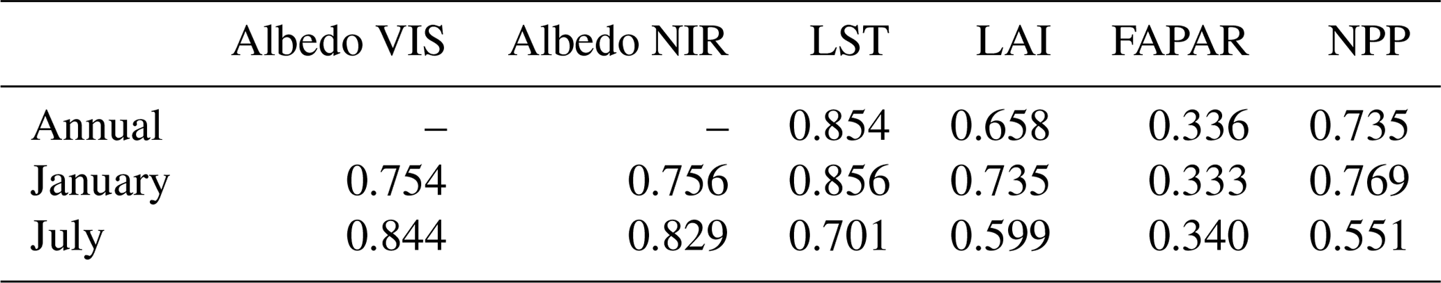
Taylor (2001) proposed a graphical way to depict the overall performance of a model. The corresponding Taylor diagram for JSBACHv4 and JSBACHv3 is shown in Fig. 1. The LST achieved by far the best agreement of the statistical metrics with observations. These metrics remained nearly unchanged from JSBACHv3 to JSBACHv4. Except for the LST, all standard deviations are reduced in JSBACHv4 (especially FAPAR). Overall, some statistical metrics of JSBACHv4 improved, while others worsened as compared to JSBACHv3. Thus, the overall performance remained more or less the same. This is also visible in the NME in Tables A1 and A2, where the NME magnitude is very similar between the assessment variables of both models.

Figure 1 Taylor diagram (Taylor, 2001) of the normalized pattern statistics for annual means of our main evaluation variables of LST, LAI, FAPAR, NPP, and WUE. The diagram contains no values for albedo because, during polar winters, observations are missing. JSBACHv3 is shown with small dots and JSBACHv4 with big darker dots. Arrows indicate the change from JSBACHv3 to JSBACHv4. The centred pattern root mean square error (RMSE) and standard deviations have been normalized by the observed standard deviation of each field before plotting. Correlations are depicted by lines from the origin representing angles relative to the horizontal base line. Standard deviations are represented as arcs around the origin. Normalized centred pattern RMSE values are seen as circular arcs around the value 1 of the baseline (normalization on standard deviation 1.0).

3.2 Albedo

Figure 2 shows, for both JSBACH versions, the albedo biases, which are given separately for the visible (VIS) and near-infrared (NIR) range. The bias pattern is very similar for JSBACHv3 and JSBACHv4, with exceptions only found in central North America and some regions in northeastern Europe (e.g. in the January values of the VIS albedo). The similarity of bias patterns between the two model versions is visible in Table 3. It is also visible from the scatterplots in Fig. B2. The correlations (r and rho) are about 0.7 and higher, except for r∼0.6 for VIS albedo in January when a larger scatter arises from polar regions.

Figure 2 Bias in white sky albedo (WSA) for JSBACHv4 (left) and JSBACHv3 (right) compared to MODIS data averaged over the years 2001 to 2014. Shown are the biases in the near-infrared (NIR) and visible (VIS) range for January and July. Because of polar night, no observation data are available for the Arctic and Antarctic winter. Note that significance is not shown because nearly all differences are significant (p=0.05), according to an independent two-sample t test.

Table 3 Spatial Spearman rank correlations (rho) between the biases of JSBACHv4 against those of JSBACHv3 for all grid cells.

For the biases seen in Fig. 2, three main causes can be identified. First, the too low VIS albedo and the too high NIR albedo over glaciers (Antarctica and Greenland) is likely a direct result of the fixed minimum and maximum albedo values used in the JSBACH calculations of glacier albedo. Second, the strong negative VIS and NIR albedo bias seen for January in western North America, eastern Europe, and large parts of central Asia is most probably a result of the bias in the dynamically calculated snow cover fraction (compare Fig. 3). And third, the biases in all other regions that are not covered by glacier or snow are at least partly caused by old canopy and soil albedo maps used in JSBACH. These biases will be explained in the next paragraph.

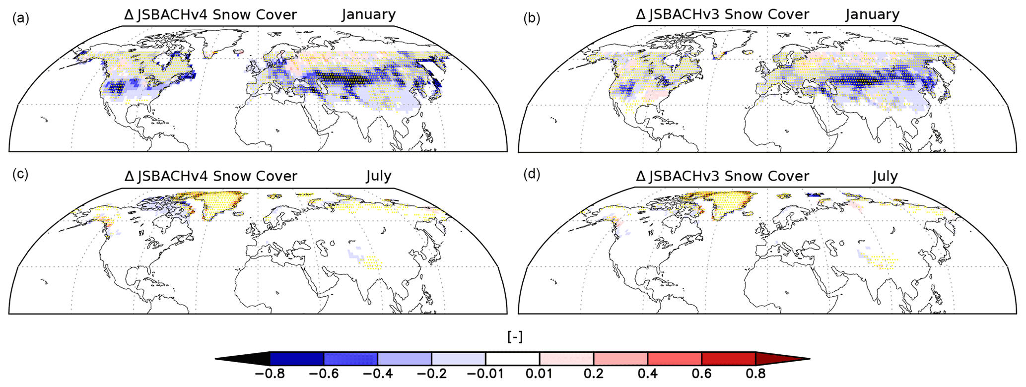
Figure 3 Bias in snow cover for JSBACHv4 (a, c) and JSBACHv3 (b, d) compared to MODIS data. Shown are the averages of January (a, b) and July (c, d), which have been averaged over the years 2001 to 2014. The yellow dots indicate the grid boxes where the bias is significant (p=0.05) according to an independent two-sample t test.

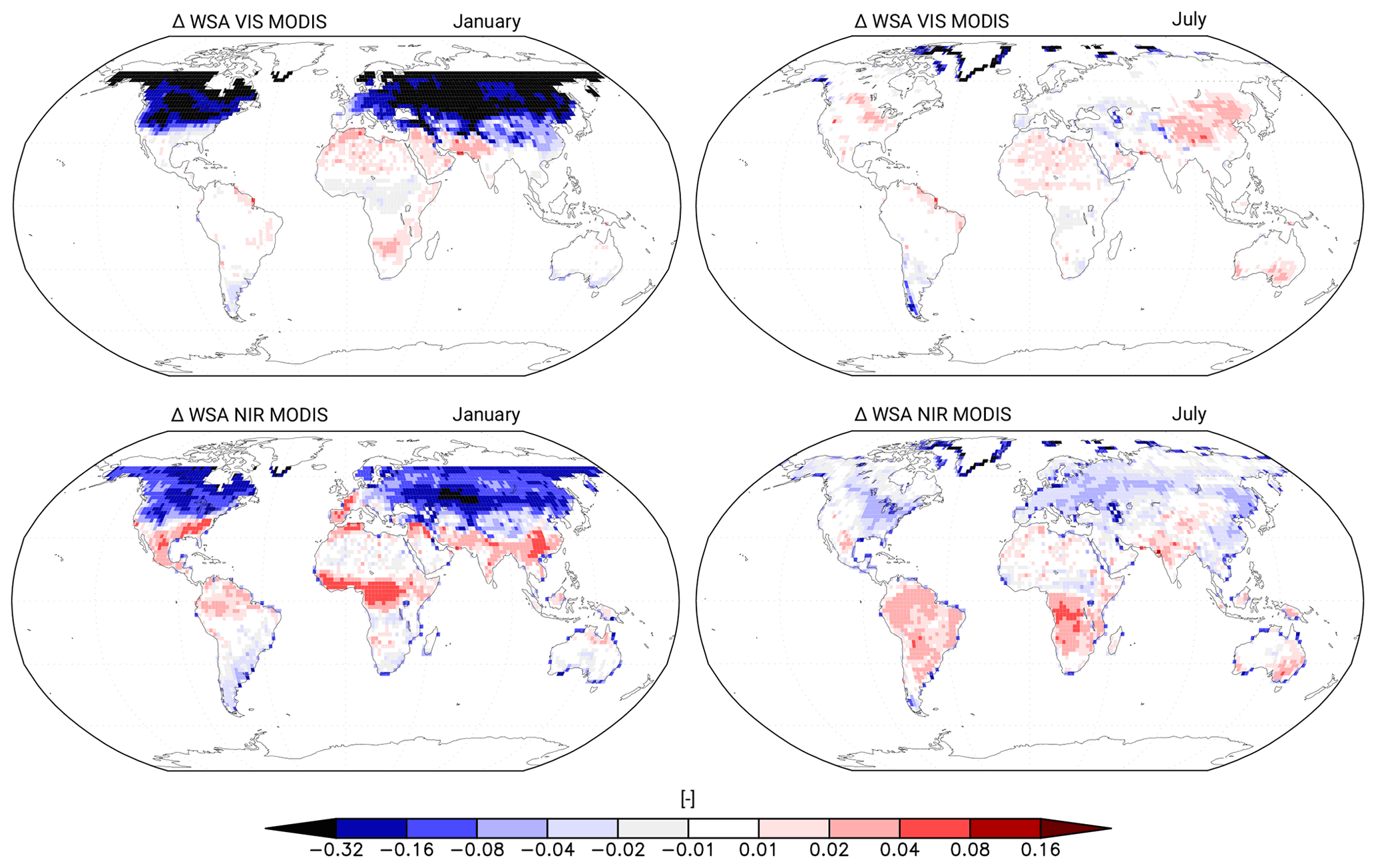
Figure 4 Difference in white sky albedo (WSA) between the two versions of MODIS data averaged over the years 2001 to 2014. The older one, from which the soil albedo maps used in JSBACH were derived, and the newer one, used for our bias analysis in Fig. 2, are shown. Also shown are NIR and VIS. As JSBACH does not account for seasonality in the soil albedo maps, the old version is a yearly mean. From this version, we subtracted the January and July values of the newer version. The differences shown here can be interpreted as the bias of JSBACH compared to the observations for January and July.

Our analyses reveals that the reason for the too low NIR albedo obtained for northern midlatitudes summer is the static map used for soil albedo. The origin of the mostly too large albedo values in other regions (South America, Africa, India, and Australia) are not traceable to single causes but must be a geographically complex result of the calculated superposition of the assumed values for canopy albedo (which depend on vegetation type) and the static map for soil albedo. A closer inspection (not shown) indicates that, in the NIR range, JSBACH has too high a canopy and too low a soil albedo, while, for VIS albedo, the converse must be suspected. JSBACH uses the same canopy and soil albedo maps for the whole year and does not incorporate seasonality. The canopy and soil albedo maps used in JSBACH are derived from a fit (see the discussion in Sect. 4.2 for details) to the 2001 to 2004 mean of an older MODIS product (MODIS MOD43C1 CMG Collection 4 Albedo product; Strahler et al., 2021; Gao et al., 2005). As the version used internally in JSBACH is a yearly mean, one would expect strong differences in observations for January and July. In Fig. 4 we show the difference between the version used internal in JSBACH and the MODIS observations for January and July that we use here for our bias analysis. These differences explain a considerable part of the albedo biases seen in Fig. 2. In Africa, for example, for both months considered and both spectral ranges analysed, large parts of the JSBACH biases are already visible as the bias of the older compared to the newer MODIS product. The same holds for southeastern Asia and for the NIR albedo in India. Accordingly, a considerable part of the biases in albedo arises from the maps for canopy and soil albedo. Note that the rather large differences between the two albedo products seen in Fig. 4 at high latitudes in the Northern Hemisphere winter in the visible range are irrelevant for our analysis here because, in these regions at that time of the year, the values from the static maps of soil and canopy albedo do not enter the calculated albedo value in JSBACH because of the snow there.

3.3 Land surface temperature (LST)

Global mean LST of 9.6 ^∘C simulated by JSBACHv4 matches well with observational data (see Fig. 5 top). The lower Northern Hemisphere winter values found for JSBACHv4 (Fig. 5 bottom) are the main reason for the overall about 1 ^∘C colder climate compared to JSBACHv3 and the better fit with the MODIS data. For JSBACHv4, the values for January are up to 2 ^∘C lower than for JSBACHv3, otherwise the seasonality is very similar for the two model versions, and the phasing is consistent with MODIS observations.

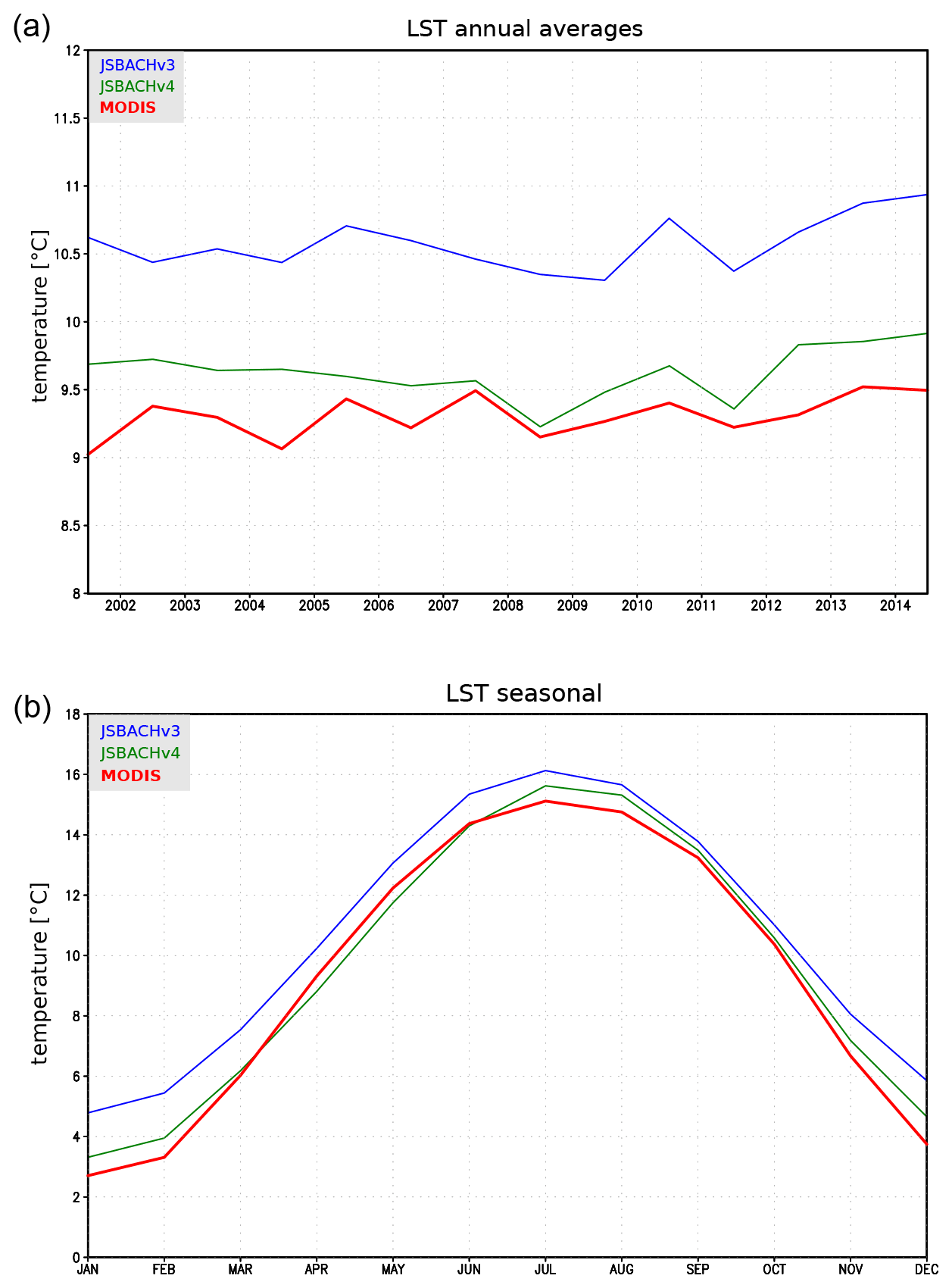
Figure 5 Global mean LST for JSBACHv3, JSBACHv4, and observation values from MODIS. (a) Annual averages from 2001 to 2014. The vertical grid lines indicate 15 January of the respective year. (b) Monthly mean values over the time period form 2001 to 2014. The vertical grid lines indicate the 15th of the respective month.

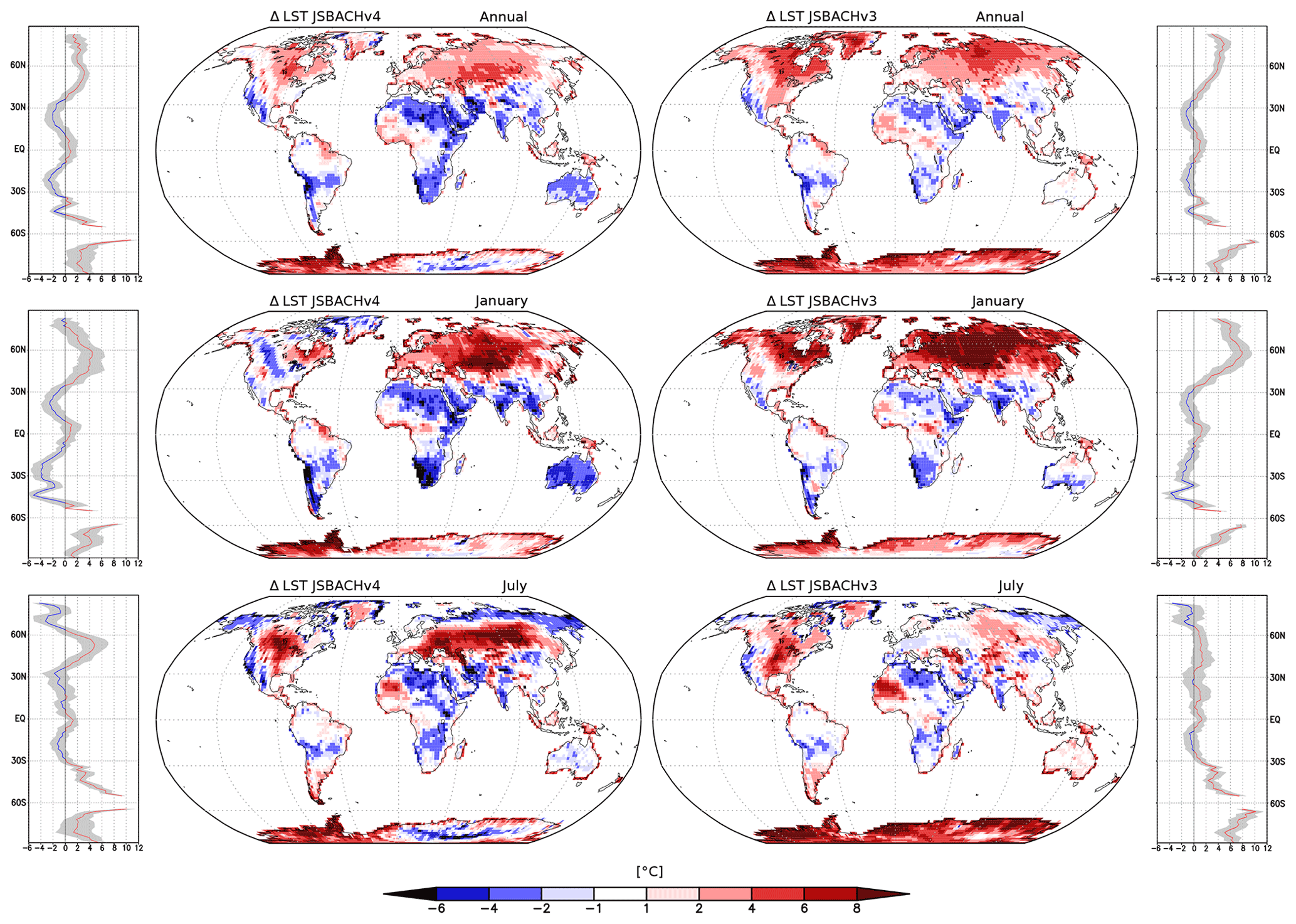
Figure 6 Bias in land surface temperature (LST) compared to MODIS data averaged over the years 2001 to 2014. Shown are the annual averages (top row) and the averages of the Januaries (middle row) and Julies (bottom row). The zonal and spatial plots in the left two columns refer to JSBACHv4, while those in the right two columns refer to JSBACHv3. The grey range in the zonal plots indicates the 95 % uncertainty range calculated from a Student t distribution, so that zonal values are significantly different when the zero-bias line is found outside this grey range. Note that the significance for the grid cells, from an independent two-sample t test, is not shown because nearly all biases are significant worldwide (p=0.05).

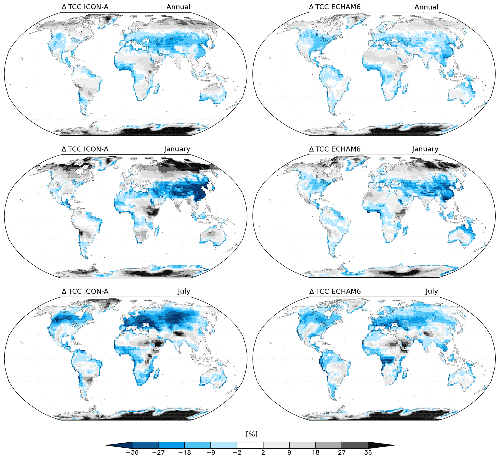
Figure 7 Bias in total cloud cover (TCC) for ICON-A (JSBACHv4) and ECHAM6 (JSBACHv3) compared to MODIS data. Shown are the annual, January, and July means over the years 2001 to 2014.

Figure 8 Bias in precipitation for JSBACHv4 (left) and JSBACHv3 (right) compared to GPCP precipitation. Shown are the annual, January, and July means over the years 2001 to 2014. Note that land areas, where the bias is smaller than the GPCP error bar, are not plotted. The yellow dots indicate grid boxes where the bias is significant (p=0.05), according to an independent two-sample t test.

In Fig. 6, we show the geographic distribution of temperature biases with respect to MODIS; to the left we show the biases for JSBACHv4 and to the right those for JSBACHv3. For both models, the strong regional biases cancel each other out in the global mean, leading to the relatively weak biases in Fig. 5 (top). At the annual mean (Fig. 6; top row plots), the geographic distribution of temperature biases is very similar for the two models, and their difference is typically smaller than the bias. The zonal plots to the left and right reveal that the higher northern latitudes warm bias is also significant when considered to be a large-scale phenomenon (for regions north of 45^∘ N, the uncertainty range seen in the zonal plots lies off the line of the zero bias). This temperate to boreal warm bias is, for both model versions, visible during Northern Hemisphere winter (see the middle row plots for January) but less strong for JSBACHv4. In July, the bias is much more pronounced in JSBACHv4 (mainly around 50^∘ N; also visible in Fig. B3) and, in contrast to JSBACHv3, significant in the zonal mean (see Fig. 6). In January, the above-named snow–albedo feedback surely contributes to the warm bias in JSBACH. In July, the negatively biased JSBACHv4 precipitation (Fig. 8) obviously supports the warm bias in Eurasia through the associated evaporation reduction (Table A3 shows a correlation of ∼ −0.6). Table 4 also shows a high correlation (∼ −0.8) between the JSBACHv4 July LST bias in Eurasia and a weaker total cloud cover (TCC; see Fig. 7). It seems obvious that the JSBACHv4 biases in this area are the result of a feedback loop, as too few clouds and too little precipitation result in too low soil moisture (SM) and evaporation, which feeds back to precipitation and is associated with the too high LST. In the following, this will be called the precipitation–SM feedback. It is probably caused by the frozen soil and five-layer snow scheme implemented in JSBACHv4 (see the discussion in Sect. 4.3 for details). In contrast, in JSBACHv3, the precipitation–SM feedback seems to have no importance in this region. Instead, the January warming effect of the TCC is more pronounced in JSBACHv3 (see Table 4). However, for both models, a higher TCC has a warming effect in January – as expected from the general rule that a cloud cover tends to warm the surface in winter (Chen et al., 2000).

The Antarctic and Greenland ice sheets tend to be warm biased (see the annual averages in Fig. 6). Only JSBACHv4 in January in Greenland shows no uniform pattern. Cold biases are seen in the northern and southern subtropics and are more evident for JSBACHv4. These two observations together – lower high-latitude warm bias and stronger subtropical cold bias – are the reason for the globally lower temperature seen for JSBACHv4 in the plot of Fig. 5 (top). This is somewhat more pronounced for January, which is visible in the zonal averages and in Fig. 5 (bottom).

The differences in bias patterns between the two model versions are also visible in the scatterplots of Fig. B3. The low July correlation (r=0.653) is caused by JSBACHv4 being warmer in the temperate zone and colder in the polar zone (for a definition of the zones, see Fig. B1). For January and also for the whole year, LSTs are much more strongly correlated (r>0.84). This is also true when we regard the corresponding rank correlations of Spearman (Table 3).

Overall, for both models, the bias pattern is very zonal, showing a warm bias at northern and southern higher latitudes, a cold bias in the northern and southern subtropics, and an insignificant bias in the equatorial regions (Fig. 6). The north–south symmetry of this zonal bias pattern hints at an atmospheric origin in the simulated climate, since, for biases caused by land processes, one would not expect a north–south symmetry because of the very different continental distribution in the two hemispheres.

In summary, we find that (1) the global mean LSTs of JSBACH only fit the MODIS data because regional biases cancel each other out. The global mean LSTs of JSBACHv4 fit better with the MODIS data because of its lower January values in the subtropics. (2) Because of the overall zonal bias pattern of both models, a strong atmospheric contribution has to be assumed. (3) Both models exhibit a higher northern latitude warm bias. In January, especially in JSBACHv3, the TCC partly causes this warming, and both models show a strong amplification by the snow–albedo feedback. In July, but only in JSBACHv4, a feedback between precipitation and SM causes a warm bias. (4) Except for Greenland in January for JSBACHv4, the Antarctic and Greenland ice sheets tend to be warm biased.

Table 4 Spatial Spearman rank correlations (rho) between the JSBACHv4 and JSBACHv3 biases of TCC against those of LST and FAPAR.

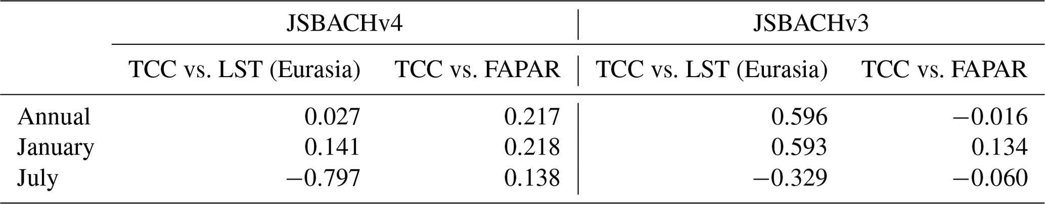
Eurasia refers to the square between longitude 0–184^∘ and latitude 35–90^∘.

3.4 Terrestrial water storage (TWS)

Figure 9 shows the agreement between JSBACHv4 and GRACE in the alterations in TWS changes in the course of the year. The strongest differences occur in dry regions with small TWS changes. In these regions, precipitation is very sensitive to the exact atmosphere dynamics, and thus, small shortcomings result in strong effects in Fig. 9. At the same time, in regions where precipitation is not very sensitive to exact atmospheric conditions, the model is in better agreement. For example, this includes the inner tropics with strong deep convection (central Africa, central South America, and northern Australia), regions that are strongly affected by the monsoon (India and Africa), and regions that are dominated by the westerlies (Europe and eastern Europe). Also northeastern Asia reveals relatively good agreements, despite the fact that the amount of TWS change is not high there. In contrast to this general rule, quite the opposite applies for the Indonesian islands. This is probably due to the resolution of the model, which cannot depict precipitation very exactly for small land areas surrounded by ocean. We find the same problem also for all extratropical islands.

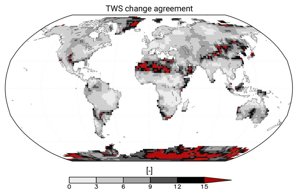
Figure 9 Normalized TWS change differences in the course of the year between the JSBACHv4 and GRACE data. Note that, due to the statistics, only the relative agreement between different regions can be rated but not the amount of water mass change agreement in absolute terms. However, the higher the value, the stronger the difference in the course of the year between JSBACHv4 and GRACE will be.

3.5 Leaf area index (LAI)

In Fig. 10, we show the bias in LAI for JSBACHv4 and JSBACHv3 compared to MODIS LAI data. The bias patterns between both models are strongly correlated (see Table 3). In the tropics, the bias pattern is quite similar. Differences between the models are mainly seen in the northern extratropics, where in July the LAI is too large for JSBACHv4 across the high northern latitudes (Canada, Alaska, and Norway) and for JSBACHv3 too large along the Eurasian steppe belt. For the latter region, this may be related to the slightly longer growth period in JSBACHv3 because of the earlier rise in Northern Hemisphere spring temperatures (see Fig. 5 bottom). The widespread and very similar significance pattern between the JSBACH versions reveals that JSBACH is systematically biased independent of the atmosphere model.

Overall, the bias is small in regions that are only sparsely covered with vegetation (e.g. northern Africa, Middle East, northeastern Asia, and central North America), and in regions with strong bias, the LAI is generally too large, as is also seen in the scatterplots of Fig. B5, where the centre data cloud is at an LAI bias of about 1. Clearly visible, particularly for JSBACHv3, is a positive LAI bias in tropical and subtropical regions with high relative soil water levels (compare Fig. 11), which is plausible insofar as it is only for good growing conditions that the LAI may overshoot. In other regions, a spatial correlation between LAI bias and relative soil water level is not as clear. The general higher relative soil moisture (RSM) in JSBACHv3 as compared to JSBACHv4 is obviously a consequence of its higher precipitation (Fig. 8).

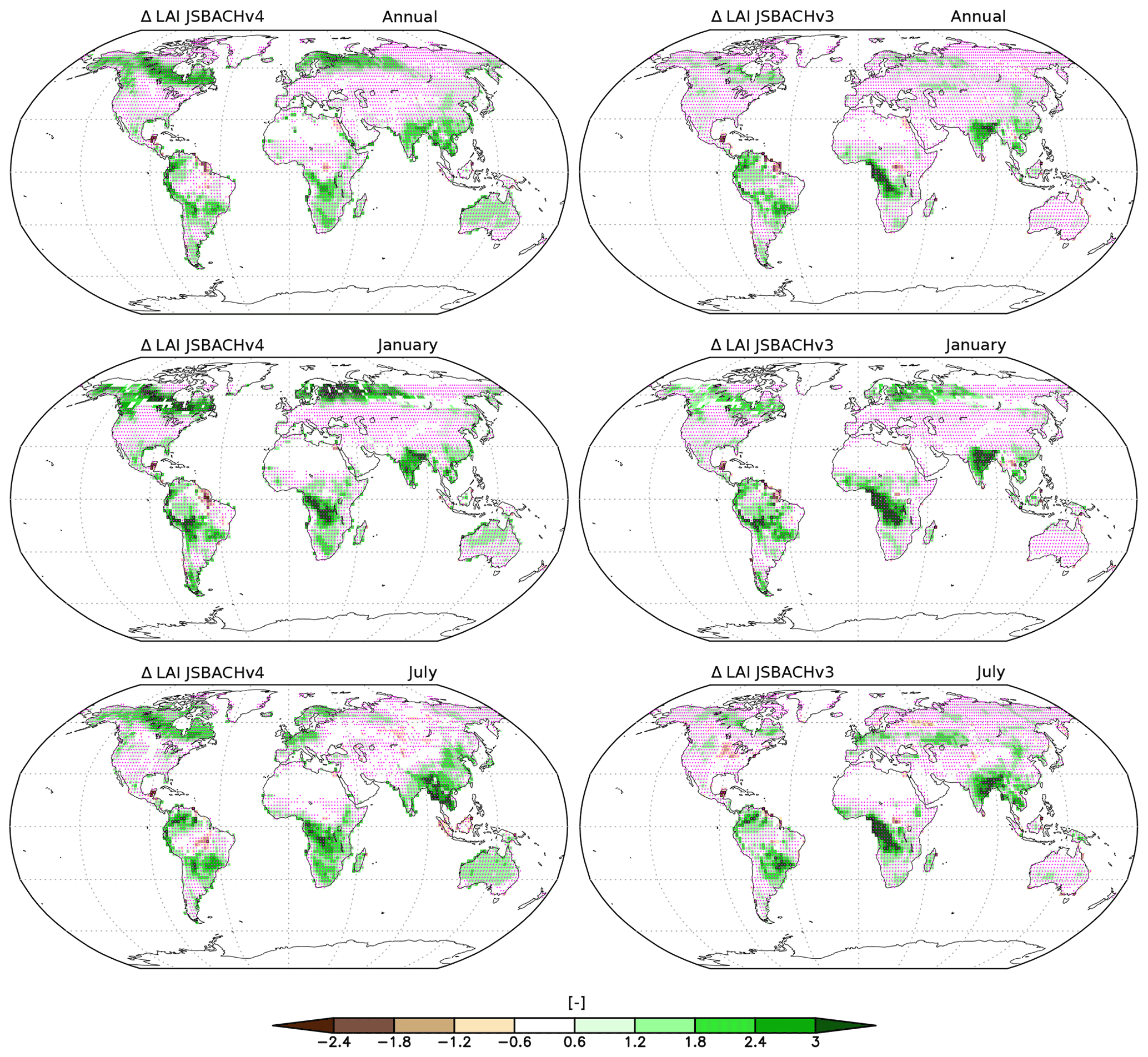
Figure 10 Bias in leaf area index (LAI) compared to MODIS data for JSBACHv4 (left) and JSBACHv3 (right) averaged over the years 2001 to 2014. Shown are the annually averaged bias and those for January and July. Pink dots indicate grid boxes where the bias is significant (p=0.05), according to an independent two-sample t test.

For a more detailed analysis of the bias patterns, one must note that JSBACH uses different parameterizations for its vegetation types to calculate the seasonal and multiannual dynamics of the LAI, i.e. to describe their phenology. These parameterizations differ in particular by their dependence on growth conditions (temperature, relative soil water, and NPP). To analyse the origin of the biases, it is therefore necessary to consider each region with its prevailing vegetation types separately. Such analysis (not shown) reveals only weak correlations between growth conditions and the diagnosed LAI biases (except for the above-named RSM). It seems unlikely that this is caused by several environmental conditions affecting the LAI dynamics simultaneously in a way that correlations cancel. It is more likely that the LAI biases are caused by shortcomings in the parameterizations of the phenology, for example, by an unlucky choice for the combination of the many parameter values, like spring growth rate for LAI and maximum length of growth season, or by more structural deficiencies, like the missing coupling between LAI and leaf biomass in this type of phenology model.

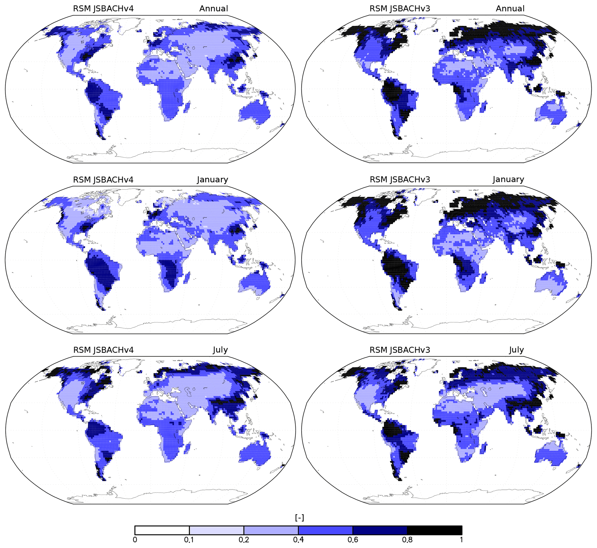
Figure 11 Relative soil moisture (RSM) in JSBACHv4 (left) and JSBACHv3 (right). Shown are the annual, January, and July means over the years 2001 to 2014. RSM is calculated as the ratio between the amount of soil water above wilting point and the amount of water between field capacity and wilting point. RSM thus characterizes the soil conditions concerning water stress of plants (the plant usable field capacity).

However, for the LAI bias of JSBACHv4 in Australia, we can indeed identify environmental causes. Australia's canopy is, especially in the areas with too high LAI, dominated by shrubs and C₄ pasture, whose phenology is calculated by the parameterizations of raingreen phenology and grass phenology, respectively. The LAI of both phenology parameterizations depends on the relative soil water level and the NPP of the model vegetation. The grass phenology additionally depends on the air temperature of the lowest atmospheric level. As the surface temperature in this area is too low throughout the year (Fig. 6), this is most likely not the cause for the positive LAI bias. In terms of simulated relative soil moisture (Fig. 11), Australia is not particularly dry. There is sufficient soil water available for plant growth in the annual average and for January and July (values range between 0.4 and 0.5). Particularly in July, the dry season of central and northern Australia is not at all represented in the simulations. As the model bias in NPP is rather weak for July (see Fig. 13), the overly wet soils should be the main reason for the too high LAI. For January, however, in reality the soil water does not limit plant growth as in July. Therefore, even though our models exhibit too much soil moisture in January, this might not cause the too high LAI. Hence, in this case, the positive NPP bias could be the cause for the LAI bias, and not vice versa.

In summary, we find that (1) the LAI bias pattern are strongly correlated between JSBACHv4 and JSBACHv3. (2) The LAI is, in general, highly biased, which occurs in regions with strong vegetation cover. (3) In Australia, for JSBACHv4, the main reasons for the high biases might be the overly wet soils in July and the too high NPP in January. (4) Except for Australia, the LAI biases are probably caused by shortcomings in the parameterizations of the phenology themselves and not by the growth conditions.

3.6 Fraction of absorbed photosynthetic active radiation (FAPAR)

In general, FAPAR biases are strongly correlated with the LAI biases (see Table 5). For JSBACHv3, the FAPAR bias pattern follows in the tropics and in regions of austral and boreal summer largely the bias pattern of LAI (compare Figs. 10 and 12), as can be expected due to the FAPAR being typically larger for deeper canopies. For JSBACHv4, this correlation is weaker but still strong in the yearly average (see Table 5). Other possible sources of FAPAR deviations are clouds because they might alter the incoming PAR or the fraction between its direct and diffuse parts. However, the comparison with the bias in total cloud cover (TCC; see Fig. 7 and Table 4) reveals no general clues for that. FAPAR deviations could also be caused by the VIS soil albedo, which is used in the JSBACH canopy radiation model as the lower boundary condition. (The biases in the JSBACH soil albedo maps were already discussed above).

Table 5 Spatial Spearman rank correlations (rho) between the JSBACHv4 and JSBACHv3 biases of LAI against those of FAPAR. The corresponding Pearson coefficients are in parentheses.

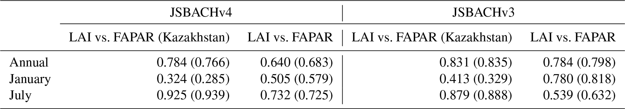
Kazakhstan refers to the square between longitude 46–87^∘ and latitude 40–54^∘ N.

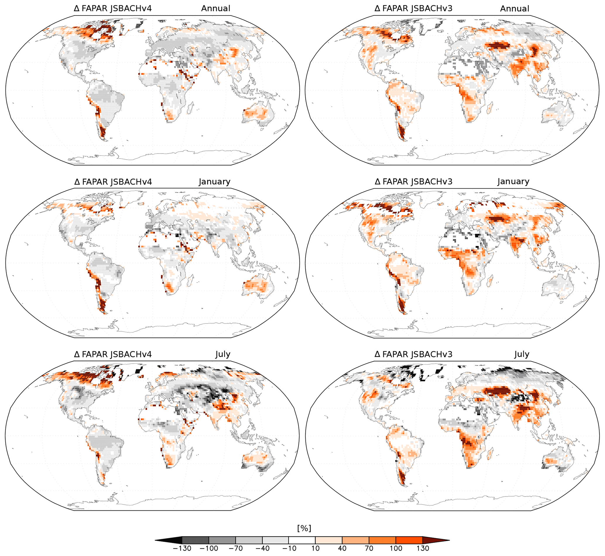
Figure 12 Bias in the fraction of absorbed photosynthetic active radiation (FAPAR) of JSBACHv4 (left) and JSBACHv3 (right) compared to the MODIS FAPAR. Shown are the annual, January, and July means over the years 2001 to 2014 (in percent) to MODIS FAPAR.

The deviations in FAPAR of the two JSBACH versions (Fig. 12) clearly differ from each other, as also reflected in the medium correlation values around 0.4 (see Fig. B6). The main differences occur over Kazakhstan, India, southern China, and central Africa. The difference over Kazakhstan (around 50^∘ N) is obviously caused by the above-described precipitation–SM feedback in July. Differences in India, southern China, and central Africa occur because the high biased LAI in JSBACHv4 does not cause the same FAPAR high bias in these regions as in JSBACHv3. As the VIS soil albedo is the same in both model versions, this cannot be the explanation. Unfortunately, our simulation outputs do not provide the necessary information about incoming PAR to verify an atmospheric origin.

3.7 Net primary production (NPP)

Except for the northern mid latitudes in the Northern Hemisphere summer, the patterns in NPP biases are very similar between the two JSBACH versions (Figs. 13 and B7). This is also demonstrated by the rather high correlations in Table 3 for the Januaries (∼ 0.8) and throughout the year (∼ 0.75), while there are lower correlation values for the Julies (∼ 0.5). In general, NPP shows strong correlations with relative soil moisture (RSM; Table 6). Only for JSBACHv3 in January are they nearly uncorrelated, which is due to the fact that, north of 60^∘, there is no NPP at that time, but JSBACHv3 has a lot of RSM. However, in general, the bias correlation between NPP and LAI is much weaker.

Table 6 Spatial Spearman rank correlations (rho) between the JSBACHv4 and JSBACHv3 biases of NPP against those of LAI, FAPAR, and RSM.

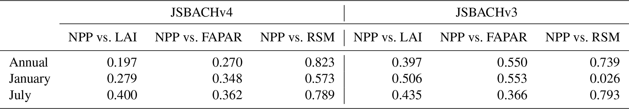
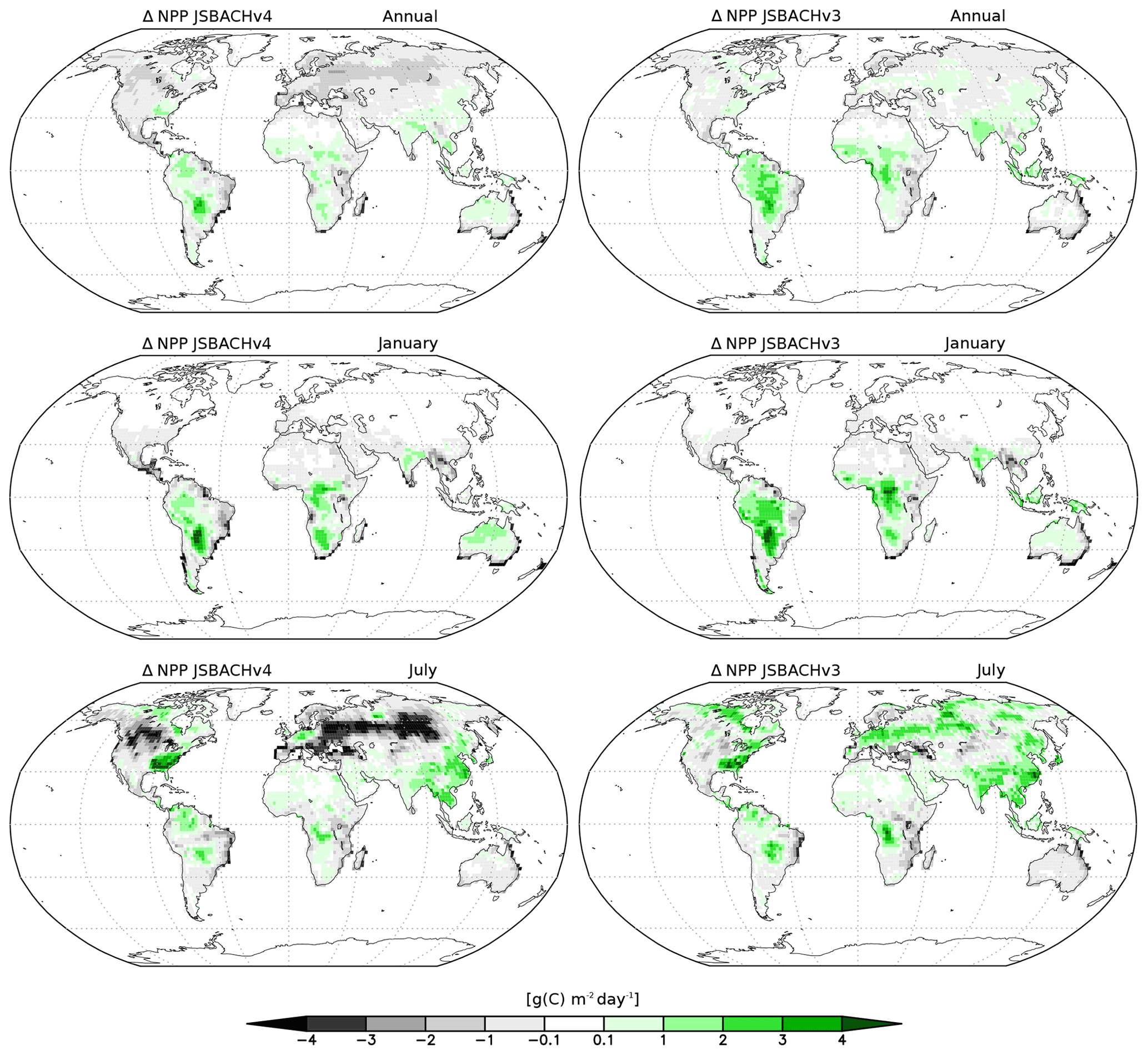
Figure 13 Bias in net primary production (NPP) for JSBACHv4 (left) and JSBACHv3 (right) compared to MODIS NPP. Shown are the annual, January, and July means over the years 2001 to 2014. Note that significance is not shown because, except for the Sahara region, all biases are significant worldwide (p=0.05), according to an independent two-sample t test.

The shift in NPP bias from JSBACHv3 to JSBACHv4 seen in northern mid latitudes in July has several reasons. For JSBACHv4, it is obvious that too low precipitation and FAPAR lead to the strong negative NPP bias (compare with Figs. 8 and 12). This bias is a side effect of the precipitation–SM feedback already explained above (similar to the LST bias for this region and time). For JSBACHv3, the bias is caused by too high LAI leading to too high FAPAR (compare with Figs. 10 and 12).

That the NPP bias is vanishing in winter for regions with seasonal vegetation is trivial, so only the patterns in summer need an explanation. For both JSBACHv4 and JSBACHv3 in the tropics and in the regions of boreal and austral summer, the bias pattern in NPP largely follows that of LAI (compare Figs. 10 and 13), which is plausible in view of the already-diagnosed positive LAI bias. The correlations between the NPP and LAI biases are not high (Table 6), as there are no correlations for the respective winter part of the globe (compare Figs. 10 and 13). The same accounts for the correlations between the NPP and FAPAR biases, although primary production directly depends on FAPAR.

In summary, we find that (1) the NPP bias pattern highly agree between JSBACHv4 and JSBACHv3, and the strongest mismatch is caused by the July precipitation–SM feedback of JSBACHv4. (2) The NPP deviations are strongly correlated with RSM.

3.8 Water use efficiency (WUE)

To discuss WUE as simulated by JSBACHv3 and JSBACHv4, we show simulation results in two ways, namely as geographic distribution (Fig. 14) and in climate space (Fig. 15). In both plots, colours are chosen to be consistent with the colour coding of the respective Figs. 1 and 2 of Sun et al. (2016) that show WUE obtained from observation data and also from simulations with other land models.

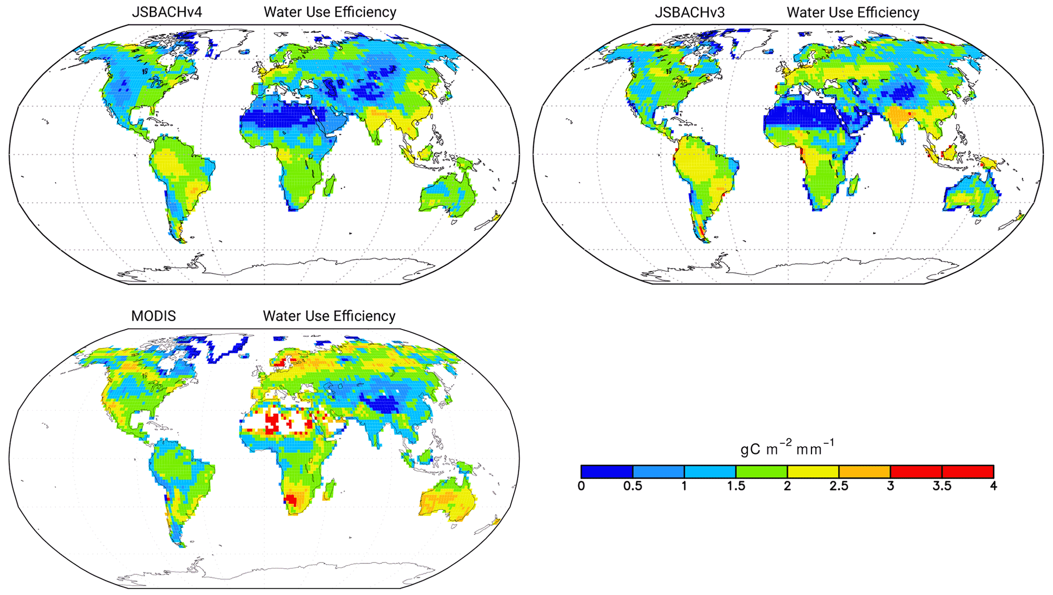
Figure 14 Water use efficiency (WUE). JSBACHv4 (top left), JSBACHv3 (top right), and MODIS (bottom left) are shown. All values are averaged over the years 2001 to 2014. The colour scale is chosen to match the one used in Figs. 1 and 2 in the study by Sun et al. (2016).

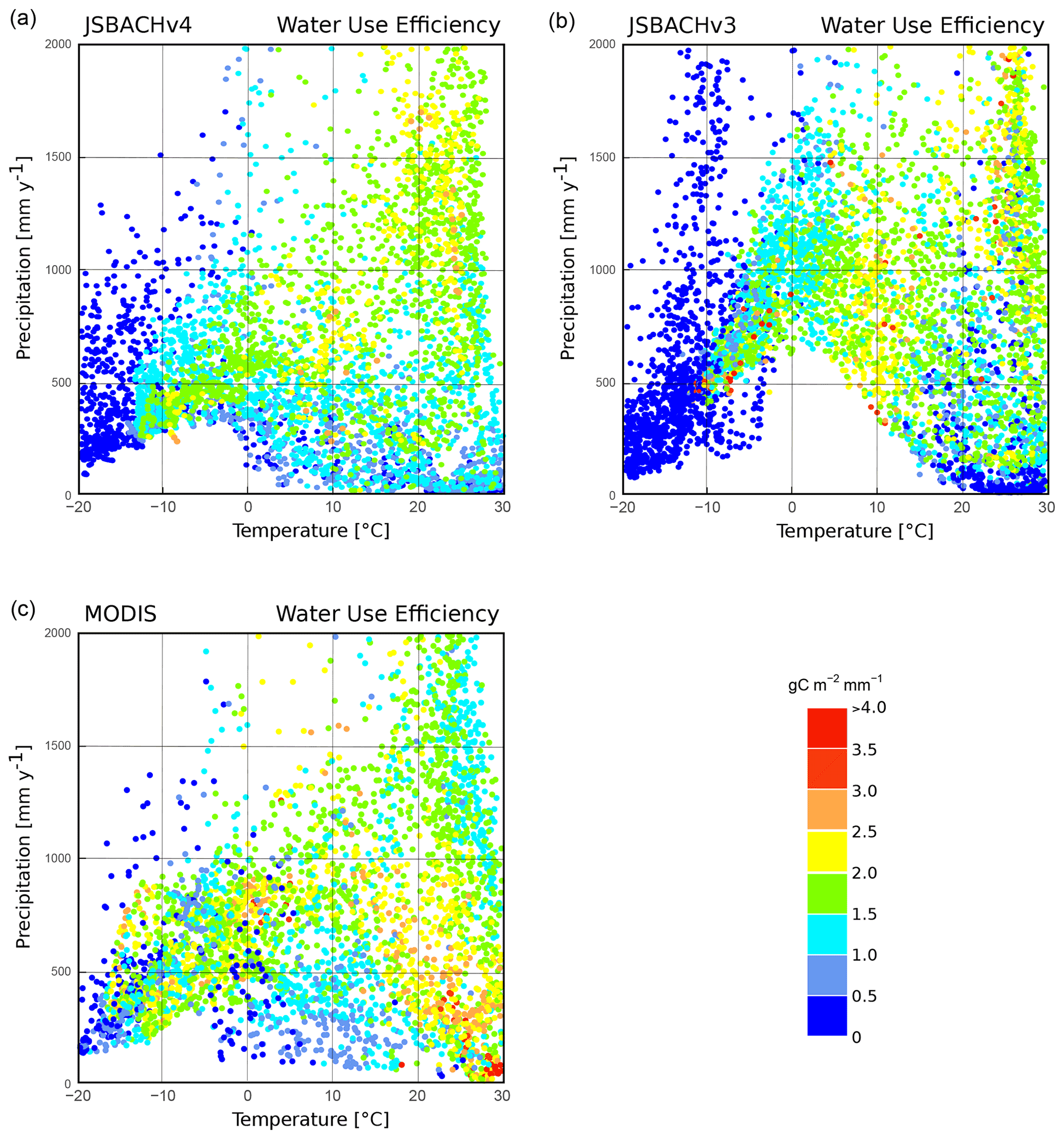
Figure 15 Water use efficiency (WUE). JSBACHv4 (a), JSBACHv3 (b), and MODIS (c) are shown for each grid cell plotted against annual 2 m temperature and precipitation. All values are averaged over the years 2001 to 2014. Colour scale as in Fig. 14.

Looking first at the geographical distribution (Fig. 14), WUE turns out to be slightly weaker worldwide in JSBACHv4 than in JSBACHv3, but otherwise, the pattern is similar. A major difference between the model versions is the rather low WUE of JSBACHv4 found in the agricultural belt along the Eurasian steppe regions, where, in the models, vegetation consists of crops. (Note that there is no correlation with the additional C₄ crops PFT of JSBACHv3.) Causal for this is the lower GPP of JSBACHv4 in this region (not shown but also visible and somewhat less pronounced in NPP; Fig. 13).

The large-scale pattern is best characterized by noting that JSBACH reveals low values for WUE in western North America, northeastern Canada, and in the broad belt ranging from the Sahara deep into inner Eurasia; elsewhere, WUE is considerably larger. The reason for this pattern is obvious from Fig. 11, showing the relative soil water content above wilting point. RSM is therefore a measure of the water stress experienced by the vegetation in JSBACH, and regions of high water stress broadly match the regions of low WUE. Accordingly, it is the low plant productivity that determines the regions of low WUE. Nevertheless, in the hot deserts – which make up large parts of the regions of low WUE – high potential evaporation surely adds to WUE being small there.

This large-scale pattern is also broadly consistent with the MODIS WUE (Fig. 14 bottom left). In contrast to JSBACH MODIS exhibits the highest global values over the dry areas in northern and southern Africa and in Australia. Sun et al. (2016) calculated the WUE from MODIS GPP and JUNG GPP (their Fig. 1a and b; the invoked evapotranspiration data are the same). The WUE calculated from their MODIS dataset is unsurprisingly very similar to our MODIS WUE and shows the same high values in these dry areas. However, the JUNG data (Sun et al., 2016; Fig. 1b) show rather low values for these regions and are therefore in much better agreement with JSBACH. A general disagreement between all observation-based datasets and JSBACH occurs in India. The too high WUE simulated for India is caused by the PFT C₃ crops. In this region, C₃ types (C₃ grass, C₃ pasture, and C₃ crops) are the most productive PFTs, and among these C₃ crops are, in terms of area, the most dominant PFTs.

Regarding the distribution of our WUE in a climate space spanned by temperature and precipitation (Fig. 15), the results of JSBACHv3 are very similar to JSBACHv4. ECHAM6 (JSBACHv3) shows much higher precipitation in the temperature range around −15 and 15 ^∘C. As a consequence, JSBACHv4 fits much better in this range than JSBACHv3 when compared to our MODIS data or to Sun et al. (2016, their Fig. 2a and b). The above-mentioned much higher global values over dry areas in MODIS as compared to JSBACH are also visible here. MODIS has its highest values in the high temperature low precipitation corner, which is the opposite in both JSBACH versions. The JSBACH Indian high bias is visible at 25 ^∘C and precipitation above 1000 mm yr⁻¹.

4 Summary and conclusions

4.1 General performance

The Taylor diagram shown in Fig. 1 and the comparison of the NME for our assessment variables (see Appendix A1 and A2) reveal that the overall performance of JSBACHv4 remains more or less as in JSBACHv3. In the context of its totally new infrastructure and the new ICON-A atmosphere, this is a good achievement and lays the groundwork for a further development of JSBACH.

4.2 Albedo

As compared to the JSBACHv3 results, JSBACHv4 shows very similar biases (and significances). Overall, the representation of the albedo in JSBACHv4 is as good as for JSBACHv3.

Nearly all albedo deviations of JSBACH are significant. In Antarctica and Greenland, the albedo deviations are uniformly too high for NIR and uniformly too low for VIS. Therefore, these deviations can be mitigated without side effects within the JSBACH calculations of the glacier albedo. For glacier albedo, values are used that vary as a function of temperature continuously between fixed minimum and maximum values. Adapting these minimum and maximum values alone should already reduce the bias, and tuning the temperature dependency could further improve the results. In the northern mid latitudes, the January albedo of JSBACH is low biased and is largely caused by a too small snow cover. It is probable that the already existing initial warm bias of ICON-A in these areas (see LST) is enhanced by the snow–albedo feedback. Tuning the snow scheme in JSBACH towards more snow might compensate the warm bias of ICON-A. However, there could be undesired side effects, such as a cold bias in eastern North America, a delay of the spring point, or too little soil water.

The JSBACH albedo bias in other regions is at least partly caused by canopy or soil albedo biases. Another source could be that the scheme merging them to the overall albedo causes additional deviations. For example, this may be related to the wrong fractions of bare ground below vegetation that are visible for the Sun or the wrong fraction of soil below the vegetation which is covered by stems but not by the LAI. However, we found that the JSBACH albedo bias in these regions can be largely explained by the canopy and soil albedo of the model. In the present model configuration, the values for the canopy are calculated from PFT-specific leaf albedo values, which themselves do not account for seasonality. The NIR and VIS soil albedos in the present model configuration are taken from prescribed maps, which also do not account for seasonality. The albedo values for the leaves and for the soil are derived by the linear regression of the FAPAR on total surface albedo (described in Otto et al., 2011). Thus, both the canopy and soil albedo values within JSBACH are based on the 2001 to 2004 average of the MODIS MOD43C1 CMG Collection 4 Albedo product. We showed that the differences between this product and the January/July values of the MODIS product used for our assessment already explain large parts of the JSBACHv4 albedo deviations. Therefore, as a first mitigation step, the MODIS database for JSBACH should be updated, and a seasonality for leaves and soil should be introduced in the JSBACH albedo scheme. Only after that would it make sense to investigate improvements in the scheme that merges snow, canopy, and soil albedo to the overall albedo.

4.3 Land surface temperatures

Overall, JSBACHv3 and JSBACHv4 show very similar temperature biases. The global mean LST simulated by JSBACH match well with observational data, especially for JSBACHv4 (see Fig. 5 top). However, this is only because strong regional biases mutually cancel each other out. The overall zonal bias pattern of both models hints at a strong atmospheric bias contribution. We find, for both models, a large-scale warm bias throughout the year over central Asia, which is also significant in the zonal averages. One reason for this is the warming effect of the TCC in January, which is enforced by too small snow cover and the snow–albedo feedback in this region. For JSBACHv4, an additional feedback between low precipitation and low RSM causes a strong warm bias in July. It is almost certain that this feedback is caused by the combination of the five-layer snow and soil water freezing schemes implemented in JSBACHv4. The effect of this scheme on the JSBACH results is analysed in detail by Hagemann et al. (2016) and is in very good agreement with our results. For the predecessor model ECHAM5, similar Northern Hemisphere winter and summer warm biases to those in our results are already shown in Ozturk et al. (2012), while the January and July biases shown in Piani et al. (2010) agree only partly (Kazakhstan and northern China). We also find too high temperatures over the Antarctic and Greenland ice sheets and cold-biased regions in South America, northern and southern Africa, Australia, India, and China (all significant). These biases are at least partly caused by albedo deviations. As the central Asian, Antarctic, and Greenland warm biases are directly connected to albedo deviations, they might be mitigated by the model adaptations proposed above for the albedo.

4.4 Terrestrial water storage

We analysed the agreement of the alterations in TWS changes in the course of the year between JSBACHv4 and GRACE. We found that the agreement is best for regions where precipitation is not very sensitive to the exact representation of atmospheric conditions in the model (i.e. regions where precipitation underlies dominant atmospheric processes like deep convection). An implication of this result is that the representation of TWS changes in the course of the year is less dependent on soil properties like field capacity or porosity than on the atmospheric conditions. Thus, from this point of view, the enhancement of soil properties is not a main focus for the development of JSBACHv4.

4.5 Leaf area index

The patterns in LAI biases are very similar between both model versions. In general, the LAI is significantly too high in JSBACH. This is not unique for our model (see Seiler et al., 2022). For JSBACHv4 in Australia, the LAI deviations for July are probably caused by too much soil moisture and for January by too high NPP. Therefore, for July, when our model does not represent a dry season in Australia, the LAI bias would be fixed by improving relative soil moisture. For January, the LAI bias might be reduced with a mitigation of the NPP bias. Except for JSBACHv4 in Australia and the general too high RSM, the LAI biases and the corresponding growth conditions are correlated only weakly. However, as our growth conditions (temperature, relative soil water, and NPP) exhibit strong shortcomings, a first step is to enhance them. As a second step, one could reduce the LAI by adapting the parameters for the phenology growth and death rates. As the LAI has a strong influence on other processes (sensible and latent heat flux, GPP and dark respiration, canopy albedo), it would be at the same time necessary to adapt these processes to the lower LAI. Nabel et al. (2020) show that the introduction of forest age classes in JSBACHv4 also reduces the LAI bias. However, this comes with additional computational costs for the model.

4.6 Fraction of absorbed photosynthetic active radiation and net primary production

We find, for both model versions, that FAPAR deviations are mainly caused by LAI biases. Overall, all NPP deviations in JSBACHv4 can be associated with water stress problems, FAPAR, and LAI. The high biased NPP would be bettered nearly everywhere with the above-named reduction in the LAI. With this reduction, the FAPAR biases would also be reduced and contribute to an improved NPP (e.g. in southern Africa and India). Our NPP biases are strongly correlated with RSM, respectively, with water stress. Higher water stress in southern and eastern North America and central Africa would further reduce our NPP deviations. However, to avoid the strong JSBACH4 low bias in July for the mid latitudes, it would be necessary to enhance the ICON-A precipitation in this area, which is a consequence of the above-named precipitation–SM feedback.

4.7 Water use efficiency

Overall, the WUE of our models looks very reasonable. In the Sahel zone, JSBACH WUE seems to be too low compared to MODIS data, but it is possible that MODIS is too high here, especially as neither the JUNG data nor the models used in Sun et al. (2016) show the same high bias. In India, our WUE is too high. One reason for this is the strong assimilation from C₃ crops. This is also visible in the NPP high bias for India. However, a high biased productivity of C₃ crops cannot be found elsewhere. Another reason might be that JSBACH does not incorporate irrigation in our simulations, which is substantial in India, and enhances evapotranspiration. As a result, WUE in JSBACH should be higher than observed. For JSBACHv3, an irrigation scheme was already implemented (de Vrese and Stacke, 2020) and could be transferred to JSBACHv4. JSBACHv4 WUE is low biased in central Asia, which is probably caused by our low biased FAPAR. WUE in JSBACHv4 is generally somewhat weaker than in JSBACHv3, but the geographical patterns are similar. The overall temperature and precipitation range of ICON-A–JSBACHv4 and ECHAM6–JSBACHv3 is similar to the observational data, but especially ECHAM6–JSBACHv3 reveals too high precipitation in the temperature range −15 to 15 ^∘C. Therefore, JSBACHv4 performs better than JSBACHv3 when compared to observations. With a general reduction in the LAI, as proposed above, and the associated reduction in GPP, the WUE of JSBACH might become low biased.

4.8 Perspectives of JSBACHv4

Our comparison with JSBACHv3 shows that the performance of JSBACHv4 is overall quite similar to JSBACHv3. Differences can partly be attributed to the different atmospheric conditions generated from and in interaction with the atmospheric host models ICON-A and ECHAM6, e.g. differences in WUE could be traced back to differences in precipitation. In terms of process descriptions, JSBACHv3 and JSBACHv4 are almost identical. The only notable difference in simulation results arising from such structural differences concerns regional differences in surface temperature via modified feedbacks with the atmosphere that we attribute to the implementation of a multilayer snow model and freezing soil water in JSBACHv4. A few options to improve JSBACHv4 have been outlined in this paper. It should be noted that the versions of ICON-A and ICON-Land/JSBACHv4 used for this study constitute the first milestone in the development of the new ICON-ESM. The flexibility of the ICON-Land infrastructure provides the basis for further developments and improvements as the land component of ICON-ESM. The model configuration of the AMIP experiments described in this paper only use the physical and biogeophysical components of JSBACHv4. The carbon cycle and dynamic vegetation processes of JSBACHv3 have also already been ported to JSBACHv4 and can already be used to model the fully closed carbon cycle within ICON-ESM, together with the ocean biogeochemistry module. The evaluation of these processes will be addressed in future work.

Appendix A

This section provides additional tables with statistical information.

Table A1 Normalized mean error (NME) of JSBACHv4 relative to observations.

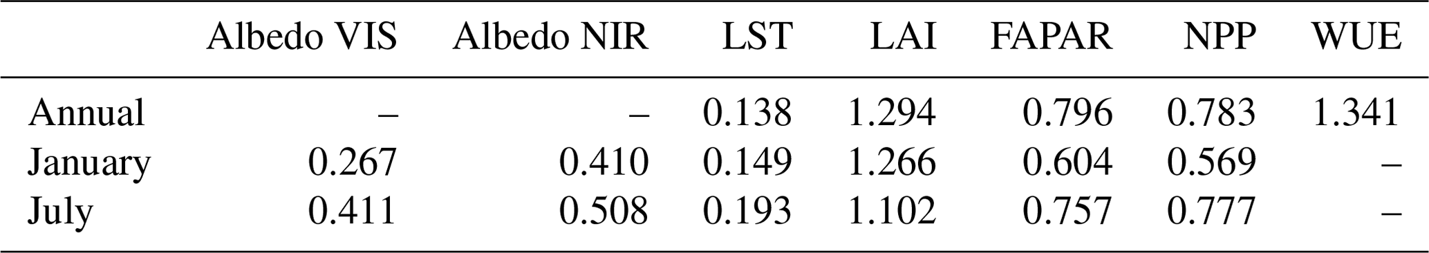
Table A2 Normalized mean error (NME) of JSBACHv3 relative to observations.

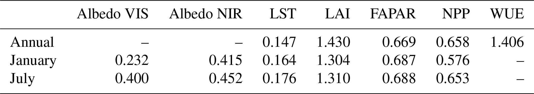
Table A3 Spatial Spearman rank correlations (rho) between the JSBACHv4 and JSBACHv3 biases of precipitation against those of LST.

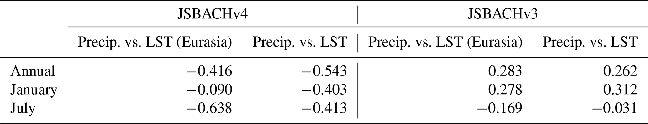
Eurasia refers here to the square between longitude 0 to 184^∘ and latitude 35 to 90^∘.

Appendix B

For a direct comparison of the simulation bias of the two model versions, we plot the difference in the observations of the various assessment variables for each grid cell of one model against that of the other here (see, e.g., the scatterplot in Fig. B3). The statistical values noted in these plots are the intercept and slope of the linear regression, the Pearson correlation r, its square R² (also called the coefficient of determination), and the Spearman rank correlation (rho). In addition, to obtain a rough idea of how the differences in simulation bias vary with region, we colourize the data points according to their broad geographical origin. For this, we distinguish the following four regions (Fig. B1):

• Polar zone (black), which is 90 to 60^∘ and −90 to −60^∘

• Temperate zone (red), which is 59.9 to 37.9^∘ and −59.9 to −37.9^∘

• Subtropical zone (yellow), which is 38 to 15^∘ and −38 to $-\mathrm{15}{}^{\circ }$

• Tropical zone (green), which is 14.9 to −14.9^∘.

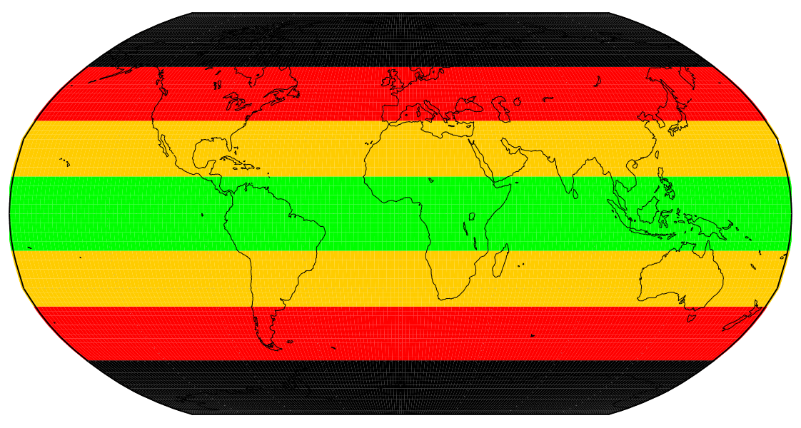
Figure B1 Zones of the scatterplots.

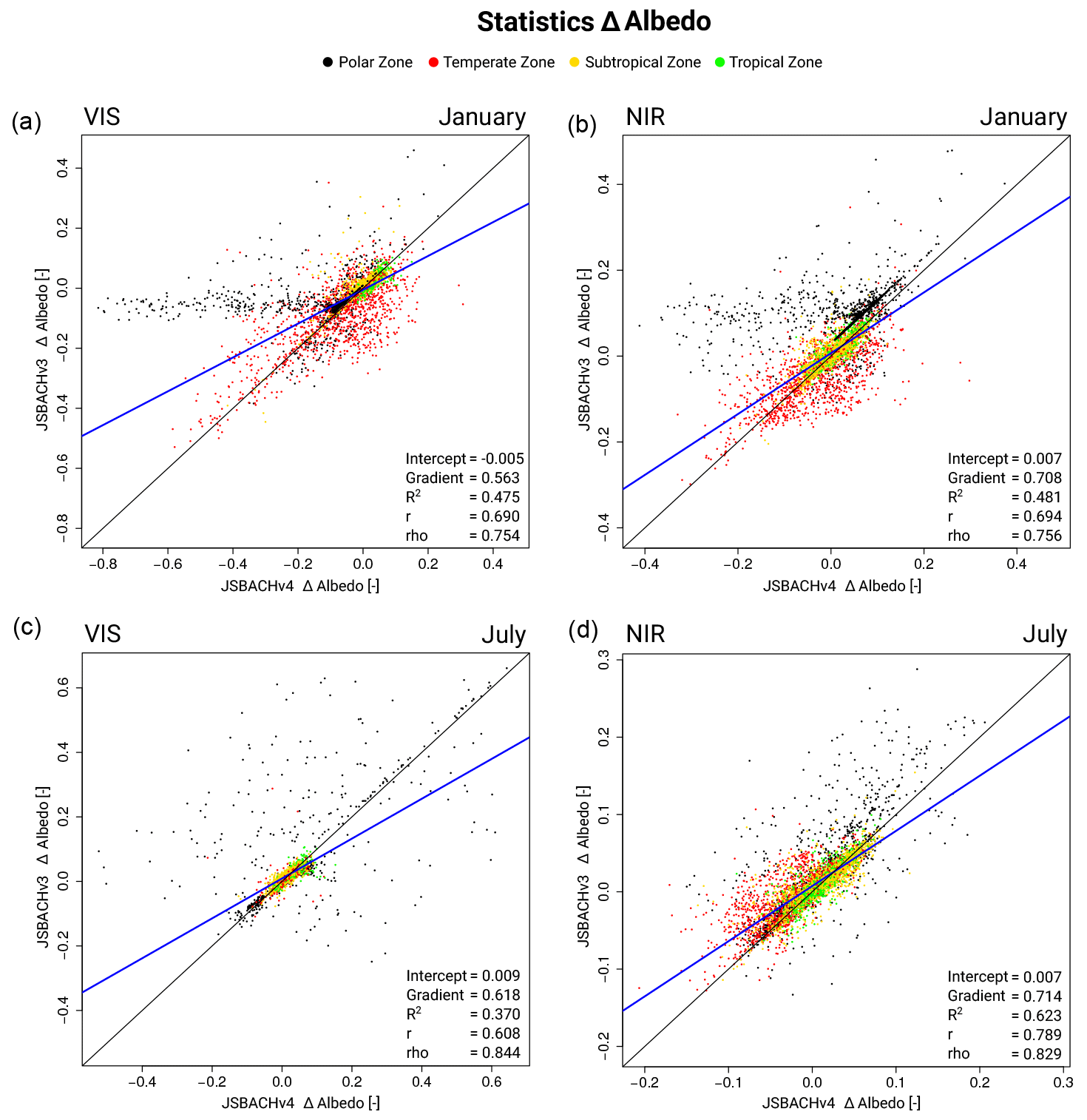
Figure B2 Comparison of simulated albedo bias (Δ albedo) between the two JSBACH versions. Plotted for each grid cell is the albedo bias of JSBACHv3 against that of JSBACHv4. The bias data are the same as in Fig. 2. Shown are the averages of the Januaries (a, b) and Julies (c, d) for VIS (a, c) and NIR (b, d) albedo. For more details, see Sect. 2.4.

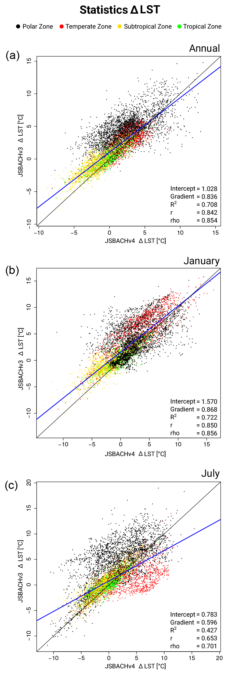
Figure B3 Comparison of simulated LST bias (ΔLST) between the two JSBACH versions. Plotted for each grid cell is the LST bias of JSBACHv3 against that of JSBACHv4. The bias data are the same as in Fig. 6. Shown are the annual averages (a) and the averages of the Januaries (b) and Julies (c). For more details, see Sect. 2.4.

Figure B4 Comparison of simulated precipitation bias (Δ precipitation) between the two JSBACH versions. For each grid cell, the precipitation bias of JSBACHv3 is plotted against that of JSBACHv4. The bias data are the same as in Fig. 8. Shown are the annual averages (a) and the averages of the Januaries (b) and Julies (c). For more details, see Sect. 2.4.

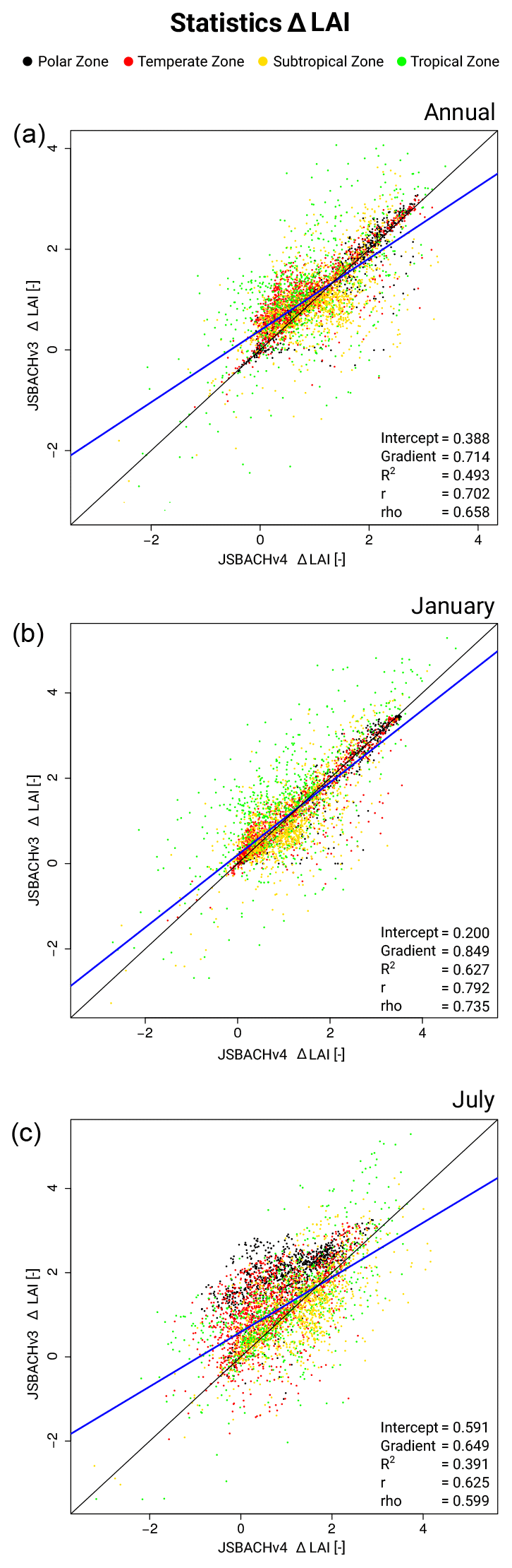
Figure B5 Comparison of simulated LAI bias (Δ LAI) between the two JSBACH versions. For each grid cell, the LAI bias of JSBACHv3 is plotted against that of JSBACHv4. The bias data are the same as in Fig. 10. Shown are the annual averages (a) and the averages of the Januaries (b) and Julies (c). For more details, see Sect. 2.4.

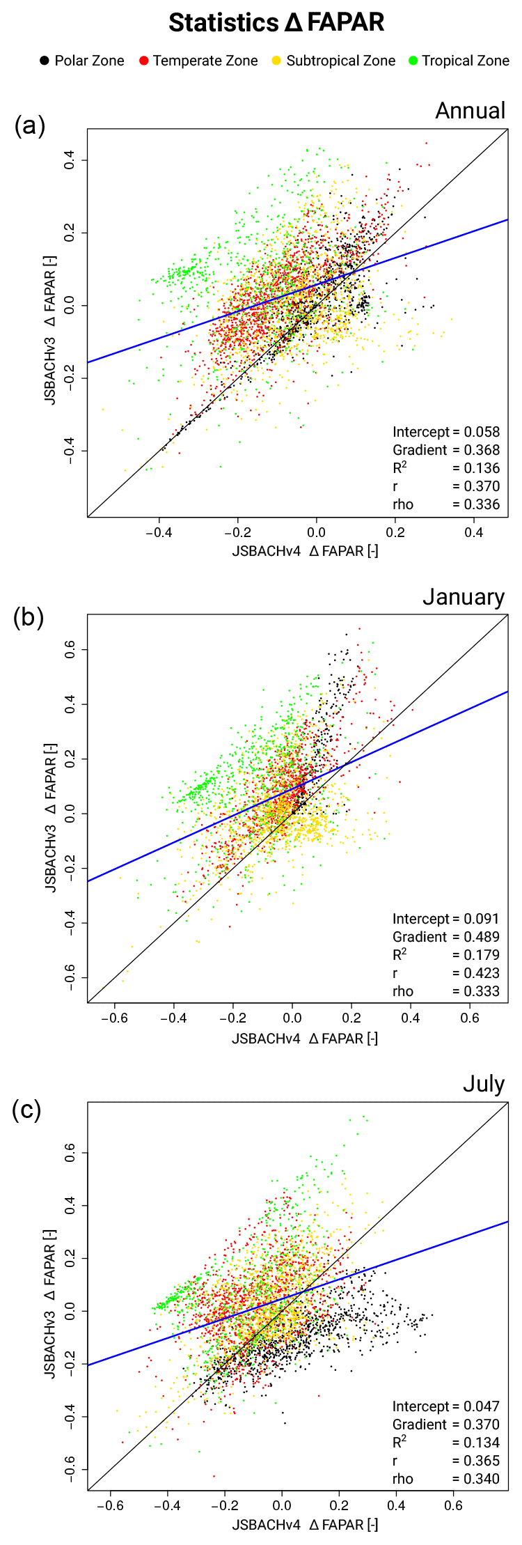
Figure B6 Comparison of simulated FAPAR bias (Δ FAPAR) between the two JSBACH versions. For each grid cell, the FAPAR bias of JSBACHv3 is plotted against that of JSBACHv4. The bias data are the same as in Fig. 12. Shown are the annual averages (a) and the averages of the Januaries (b) and Julies (c). For more details, see Sect. 2.4.

Figure B7 Comparison of simulated NPP bias (Δ NPP) between the two JSBACH versions. For each grid cell, the NPP bias of JSBACHv3 is plotted against that of JSBACHv4. The bias data are the same as in Fig. 13. Shown are the annual averages (a) and the averages of the Januaries (b) and Julies (c). For more details, see Sect. 2.4.