the Creative Commons Attribution 4.0 License.
the Creative Commons Attribution 4.0 License.
 | 21 Nov 2022
Implementation of a new crop phenology and irrigation scheme in the ISBA land surface model using SURFEX_v8.1
Simon Munier
Anthony Mucia
Clément Albergel
Jean-Christophe Calvet
With an increase in the number of natural processes represented, global land surface models (LSMs) have become more and more accurate in representing natural terrestrial ecosystems. However, they are still limited with respect to the impact of agriculture on land surface variables. This is particularly true for agro-hydrological processes related to a strong human control on freshwater. While many LSMs consider natural processes only, the development of human-related processes, e.g. crop phenology and irrigation in LSMs, is key. In this study, we present the implementation of a new crop phenology and irrigation scheme in the ISBA (interactions between soil–biosphere–atmosphere) LSM. This highly flexible scheme is designed to account for various configurations and can be applied at different spatial scales. For each vegetation type within a model grid cell, three irrigation systems can be used at the same time. A limited number of parameters are used to control (1) the amount of water used for irrigation, (2) irrigation triggering (based on the soil moisture stress), and (3) crop seasonality (emergence and harvesting). A case study is presented over Nebraska (USA). This region is chosen for its high irrigation density and because independent observations of irrigation practices can be used to verify the simulated irrigation amounts. The ISBA simulations with and without the new crop phenology and irrigation scheme are compared to different satellite-based observations. The comparison shows that the irrigation scheme improves the simulated vegetation variables such as leaf area index, gross primary productivity, and land surface temperature. In addition to a better representation of land surface processes, the results point to potential applications of this new version of the ISBA model for water resource monitoring and climate change impact studies.
- Article
(4294 KB) - Full-text XML
-
Supplement
(2853 KB) - BibTeX
- EndNote


Amongst the global water withdrawal from rivers, reservoirs, and groundwater, the share used for agriculture is estimated to reach 69 % on average, with some regional heterogeneity – over 90 % in some regions (Hoekstra and Mekonnen, 2012; FAO, 2014). This amount of water is likely to increase in the future in relation to climate warming and population growth (UNDESA, 2022; Field et al., 2014). The historical evolution of irrigation also points to increasing water consumption; the area equipped for irrigation nearly doubled from 1900 to 1950, while it tripled from 1950 to 2005 (Siebert et al., 2015).
Irrigation is used to increase crop yields by mitigating the soil water stress (Fraiture et al., 2007). Several studies indicate that yields can be higher by a factor of 2 or more when the fields are irrigated (Bruinsma, 2009; Colaizzi et al., 2009; Siebert and Döll, 2010; FAO, 2014). However, freshwater is already a limited resource, and the current evolution of irrigation has a substantial impact on (1) river discharge, with a decrease in their lower reaches due to diversions and impoundments for irrigation (Tang et al., 2008; Piao et al., 2010; Grafton et al., 2018), (2) groundwater level, with critical low levels observed in case of intensive irrigation (Rodell et al., 2009; Döll et al., 2012; Pfeiffer and Lin, 2014), and (3) the surface energy budget through an increase in evapotranspiration, which can lead to surface cooling (Kueppers et al., 2007; Lobell et al., 2008; Jiang et al., 2014; de Vrese et al., 2016). Water vapour originating from large-scale irrigation water supply can be recycled to rainfall (Moore and Rojstaczer, 2002; DeAngelis et al., 2010; Carrillo-Guerrero et al., 2013; Harding et al., 2013). It can also affect the dynamics of the monsoon (Douglas et al., 2006; Saeed et al., 2009; Shukla et al., 2014) and influence climate at both regional and global scales (Sacks et al., 2009; Puma and Cook, 2010). These findings show a gradual and significant influence of changes in irrigated areas on the hydrological cycle (e.g. Adegoke et al., 2003; Haddeland et al., 2006; Rost et al., 2008; Döll et al., 2009; Hanasaki et al., 2010; Biemans et al., 2011). The ability of numerical models to reproduce these different impacts and feedbacks is thus essential in order to understand the role of irrigation in the Earth climate system at different spatial scales (Zaitchik et al., 2005). Representing irrigation could potentially improve weather and climate forecast skill (Ozdogan et al., 2010). However, as presented below, irrigation is generally represented in models in a overly simplistic way.
Land surface models (LSMs) provide lower boundary conditions to climate and weather forecast atmospheric models. The new generation of LSMs is able to represent land surface biophysical processes and variables, including soil moisture and vegetation biomass, in a way that is fully consistent with the representation of carbon, water, and energy fluxes. LSMs differ from crop models in the sense that they neither explicitly represent all the agricultural practices nor crop yields. While most crop models have implemented irrigation, irrigation is not represented by all LSMs. Current LSMs have to improve the representation of anthropogenic factors and their interactions with natural processes (Verburg et al., 2016). In particular, LSMs need to represent the complexity of irrigation practices as much as possible, in addition to their impact on the atmosphere and on the environment. For example, efforts are made to achieve this goal in the Community Land Model (CLM), in the Noah land surface model with multi-parameterisation options (Noah-MP), in Accelerated Climate Modeling for Energy (ACME), and in ORganising Carbon and Hydrology in Dynamic EcosystEms (ORCHIDEE) LSMs (Felfelani et al., 2020; Zhang et al., 2020; Leng et al., 2017; Yin et al., 2020, respectively). As highlighted by Chukalla et al. (2015), a number of large-scale LSMs currently represent only one type of irrigated vegetation (mostly C4 crops, i.e. crops with a C4 photosynthesis carbon fixation type, such as corn and sorghum), with only one type of irrigation practice (e.g. sprinkling or flooding), for one season per year, and no interannual variability in vegetation density (Perry, 2007; Perry et al., 2009). Among others, this is the case in the current version of the ISBA (interactions between soil–biosphere–atmosphere; Noilhan and Planton, 1989) LSM, with C4 crops irrigated with sprinkling (Voirin-Morel, 2003; Calvet et al., 2008). In reality, there are a lot of different vegetation types which can be irrigated, from orchards to pastures (FAO, 2014), and different irrigation techniques with different ways to apply water (above the vegetation or directly on the ground for sprinkling and flooding irrigation techniques, respectively). Different irrigation types vary in (1) irrigation efficiency (Evans and Sadler, 2008; Jägermeyr et al., 2015), (2) the amount of freshwater used for irrigation per surface unit (FAO, 2014), and (3) impact on water resources (Khan and Abbas, 2007). Moreover, some specificities of irrigation such as the timing and frequency of water application can affect the ecosystem and atmospheric responses to irrigation (Sorooshian et al., 2012). Some models include a representation of irrigation without having an interactive vegetation scheme and using climatological values instead (such as with the Land Information System (LIS)-Noah model, a NASA land information system and LSM combination, used in Lawston et al., 2015), thereby precluding interannual variability in vegetation density and the impact of irrigation on vegetation growth. Having a more complete irrigation description is needed to reproduce the irrigation seasonality and to represent possible changes in crop phenology such as emergence and harvest dates. The impact of changing irrigation characteristics in a context of climate change could thereby be evaluated, such as increasing irrigation efficiency (currently around 56 %; FAO, 2014) and freshwater saving potential (Perry et al., 2017; Koech and Langat, 2018).
The objective of this work is to develop and evaluate a more detailed representation of crop phenology and irrigation practices into the ISBA LSM within the SURFEX (SURFace EXternalisée) modelling platform; Masson et al., 2013). The new scheme is designed to work on a global scale. We focus on a densely irrigated area in Nebraska where validation data are available.
Section 2 presents a description of the ISBA LSM, the new crop phenology, irrigation scheme, and the validation protocol, followed by a description of the observational datasets. Section 3 illustrates the impact of the new scheme when compared to simulations without crop phenology and without irrigation. An evaluation of the performance of the model is made over Nebraska. Section 4 discusses the added value and the limits of the newly implemented irrigation scheme. Finally, Sect. 5 presents the conclusions and future research directions.
2.1 The ISBA land surface model
The ISBA model (originally described in Noilhan and Planton, 1989) is a LSM developed by the research department of Météo-France (Centre National de Recherches Météorologiques, CNRM). It is embedded into the SURFEX modelling platform (Masson et al., 2013; Voldoire et al., 2017; Le Moigne et al., 2018) and can provide initial land surface conditions to various atmospheric models (e.g. ALADIN in Fischer et al., 2005) or be driven by atmospheric conditions in offline (i.e. standalone) mode. SURFEX integrates different models describing ocean and terrestrial surfaces. Over land, specific models are used to represent waterbodies, cities, and the soil–plant system. The latter is modelled by the ISBA LSM. The ISBA model can be coupled to the CTRIP model (Decharme et al., 2019; Munier and Decharme, 2022), which is specifically designed to represent water dynamics within rivers and aquifers. Only offline ISBA simulations are considered in this study.
2.2 Crop phenology and irrigation modelling concept
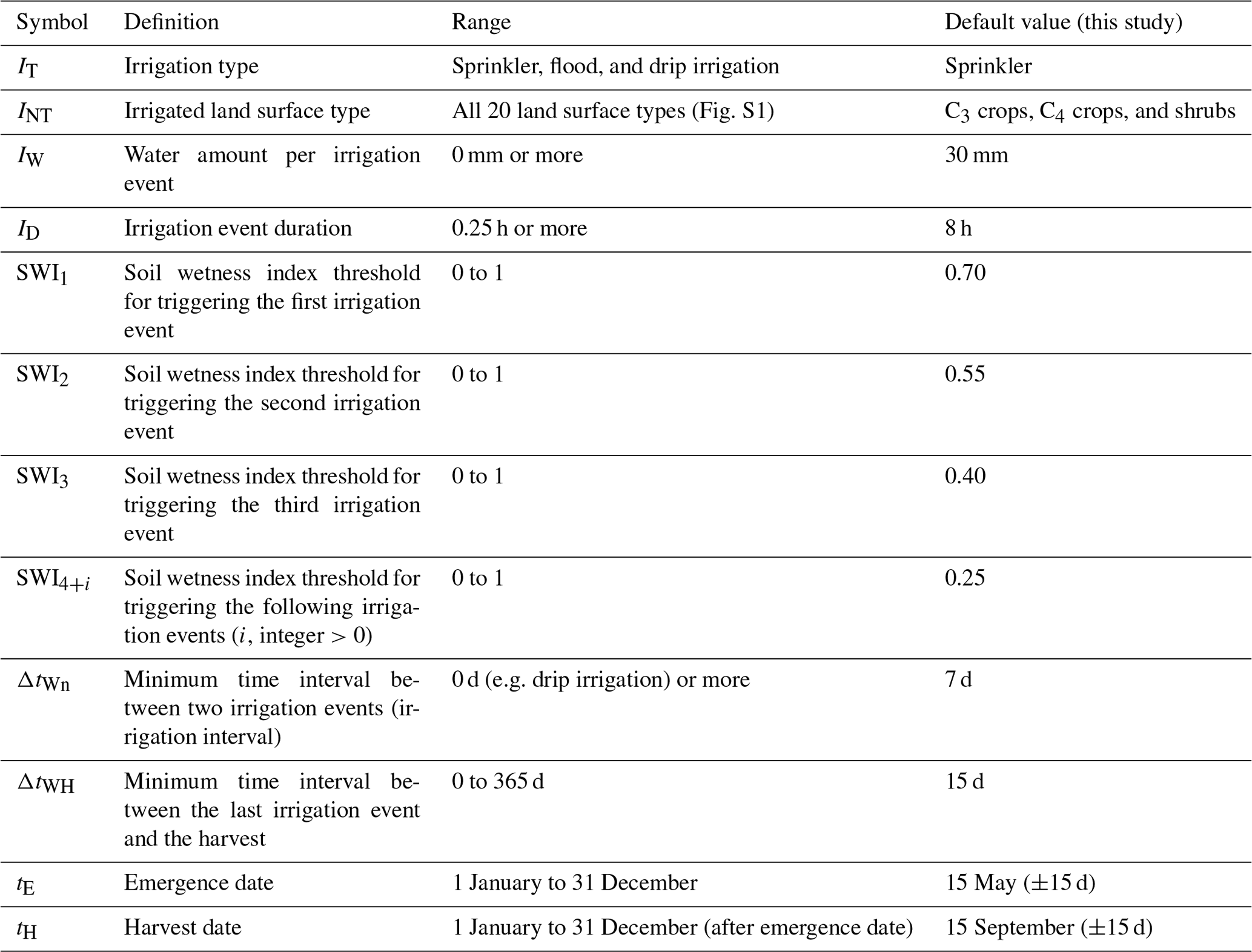
An old irrigation scheme working at a local scale (Calvet et al., 2008) is available in the ISBA LSM. Major limitations of the old scheme are the lack of (1) spatialisation on a global scale, (2) representation of harvest, (3) diversity of irrigation types and irrigated vegetation types, and (4) interoperability with the multi-layer soil hydrology scheme. Key processes implemented in this scheme are briefly described below. The irrigation can be activated for ISBA versions able to simulate photosynthesis, interactive vegetation biomass, and leaf area index (LAI; ISBA-A-gs; Calvet et al., 1998; Gibelin et al., 2006). Sprinkler irrigation is represented by imposing an additional water flux forcing to the soil–plant system. Water is applied at a given time and over a certain period of time. A number of irrigation parameters need to be assigned, such as the irrigation amount, the irrigation interval, and the irrigation start and end times. A parsimonious approach is used in order to limit the number of parameters of the model. Table 1 lists the parameters and the values used by default in the model. Using these values allows the model to predict a realistic amount of irrigation water over irrigated corn in southern France (Bonnemort et al., 1996; Voirin-Morel, 2003; Calvet et al., 2008). Irrigation is triggered using thresholds of the simulated extractable soil moisture content when vegetation growth is limited by a soil moisture deficit. The plant water stress level is evaluated using a unitless soil wetness index along the root profile (SWIroot_zone). A SWIroot_zone value close to 1 corresponds to a well-watered soil, while a value close to 0 indicates extreme stress. In order to trigger irrigation, the SWIroot_zone value is compared to predefined SWI thresholds given as input parameters. These SWI thresholds are evolving during the irrigation season, and default values are fixed to 0.7 for the first irrigation, 0.55 for the second irrigation, 0.4 for the third irrigation, and 0.25 thereafter. The use of these values was validated by Bonnemort et al. (1996), Voirin-Morel (2003), and Calvet et al. (2008). The idea behind this approach is that irrigation does not completely refill the soil, especially at the end of the growing season. Mechanical harvest requires relatively dry conditions to avoid soil compaction. The crop is allowed to use rainwater together with the initial available water content of the soil. This irrigation strategy allows the optimisation of water withdrawal according to plant water extracting abilities at different crop growing stages. When a SWI threshold is reached, irrigation is triggered with a predefined quantity of water of 30 mm (by default), following Calvet et al. (2008).
2.2.1 New crop phenology processes
In this study, ISBA-A-gs is used together with the multi-layer soil hydrology scheme described in Decharme et al. (2019). In ISBA-A-gs, phenology is entirely driven by photosynthesis, and no growing degree day model is used. The only phenology parameter is a minimum LAI value of 0.3 m2 m−2 for low vegetation. In the new scheme, specific crop phenology parameters such as emergence and harvest dates are used for irrigated crops. In practice, two dates are prescribed, namely emergence and harvest. This is a simple way to represent specific crop phenology attributes of irrigated crops. Between these two dates, irrigation is possible. Before the emergence and after the harvest, LAI is fixed at the model's minimum value (LAI =0.3 m2 m−2). The new scheme provides the option to support up to three plant growth seasons per year. The crop phenology parameters are not applied to wooded vegetation (trees and shrubs) and can be applied without irrigation.
2.2.2 New irrigation processes
In the new scheme, three irrigation types are considered, namely sprinkler irrigation, flood irrigation, and drip irrigation. The same irrigation types as in Lawston et al. (2015) are represented but a different modelling approach is used.

For sprinkler irrigation settings, the irrigation water flux is evenly distributed over a period of time of 8 h (by default) and is applied on top of the vegetation canopy like precipitation. The irrigation water can be intercepted by the vegetation canopy. The new irrigation algorithm is based on several steps described below and in Fig. 1.
First, the model determines whether fields within the grid cell can be irrigated, i.e. they are equipped for irrigation (e.g. water supply, valves, and pipes). This information is given by the irrigation map described in Sect. 2.4.1.
Second, the model checks whether the vegetation growth stage is compatible with irrigation. For crops, irrigation can be triggered after the emergence and until a few days before the harvest (by default 2 weeks).
The availability of resources (equipment or local water distribution) is taken into account through a default minimum time gap between two successive irrigations (Zhang et al., 2019). This default irrigation interval parameter value is a constant (7 d by default), but maps of irrigation intervals could be used when available.
Since a multi-layer soil hydrology scheme is used in the new irrigation model, the root zone SWI (SWIroot_zone) is a weighted average SWI value based on the soil volumetric water content profile (Wci; m3 m−3), the field capacity volumetric water content profile (Wfci; m3 m−3), and the wilting point profile (Wwilti, depending on clay and sand fraction; m3 m−3), for each soil layer i. The root fraction inside each soil layer () is used as a weighting factor as follows:
where nsoil is the total number of soil layers in the root zone. This value depends on the considered vegetation type. For example, nsoil=9 for crops with a rooting depth of 1.5 m.
In addition to sprinkler irrigation, the new model is able to represent drip or flood irrigation. In this case, the water flux is applied directly to the soil surface, without leaf interception. Considering the static equipment used for drip irrigation, there is no irrigation interval (ΔtWn=0 d). In this study, only sprinkler irrigation is considered to be the dominant irrigation type in Nebraska. Drip and flood irrigation will be evaluated in future works. The activation of a given irrigation method is described in Sect. S5 in the Supplement. Irrigation simulations are illustrated in Sects. S2 and S3 over southwestern France and over the Hampton irrigated area in Nebraska (Figs. 2e, S2, and S3), respectively. Observed monthly precipitation in Nebraska is presented for contrasting years in Sect. S4.
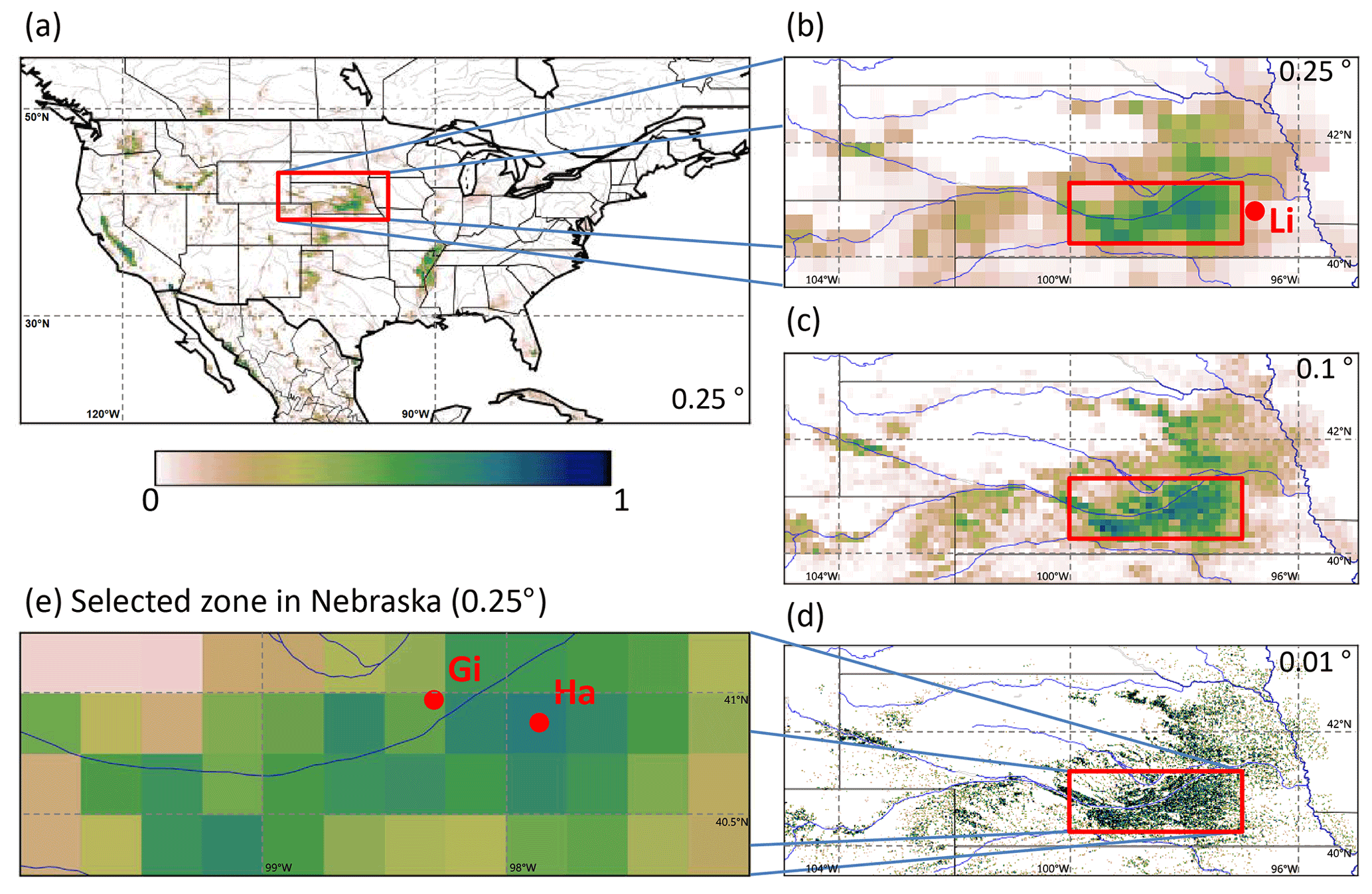
Figure 2Irrigation fractional coverage, derived from Meier et al. (2018a), over (a) the continental United State (CONUS) and (b–e) Nebraska, at (b) 0.25∘ × 0.25∘, (c) 0.1∘ × 0.1∘, and (d) 0.01∘ × 0.01∘ spatial resolutions, and (e) over the selected zone in southern Nebraska considered in this study (100–97∘ W, 40.25–41.25∘ N). The red boxes show the location of the different zooms. The Li, Gi, and Ha red dots correspond to the Lincoln weather station, Grand Island weather station, and Hampton irrigated area, respectively.
All the values of the model parameters in Table 1 have been set within a default configuration. These values can be user-defined for each land surface type and for each grid cell, including, when possible, seasonal variations. See Sect. S5 for configuration details and possibilities.
2.2.3 New aggregation rules of irrigated and rainfed vegetation
The new crop phenology and irrigation scheme is operated using ECOCLIMAP-SG to prescribe land cover (Calvet and Champeaux, 2000; Sect. S1). The best achievable spatial resolution of ECOCLIMAP-SG is 300 m × 300 m. In contrast to previous versions of ISBA, there is no specific irrigated land surface type in the new ECOCLIMAP-SG vegetation description. On the other hand, irrigation of all the 20 land surface types listed in Fig. S1 and Table S2 is possible. By default, six vegetation types are considered, i.e. three crop and three woody vegetation types (Fig. S1). The new scheme is able to represent the sub-grid heterogeneity of the irrigation fractional coverage. For example, distinct maps of the fraction of irrigated C4 and C3 crops can be produced over North America (Figs. S2 and S3, respectively). For each land surface type, an irrigated and a non-irrigated fraction are considered at the simulation resolution. In order to prevent an excessive increase in the number of simulated land surface types (potentially 20 non-irrigated and 20 irrigated × 3 irrigation types, i.e. a total of 80 types) involving a large increase in complexity, memory, and computing cost, some choices are made for the implementation.
-
Selection of a limited number of irrigated land surface types. The default implementation consists of six irrigated land surface types. Temperate deciduous and evergreen trees types (nos. 8 and 10 in Table S2, respectively) can be used to represent fruits trees or olive trees, for example, respectively. Shrub type (no. 15) can be used to represent, among others, vine plants, and types nos. 19, 20, and 21 may represent irrigated crops (e.g. wheat, soybean, and corn, respectively).
-
Selection of the main irrigation method used for each grid cell and land surface type. This option considers that, in one grid cell there is only one dominant method for a given land surface type (e.g. flooded rice in China or sprinkled corn in France).
Finally, the system state variables (soil water content, surface and soil temperature, vegetation biomass, etc.) differ in the irrigated and non-irrigated parts of the cell. This requires (1) duplicating a land surface type if it is partially irrigated, (2) attributing to the considered grid cell the corresponding fraction of irrigated surface, and (3) selecting the irrigation type for the irrigated fraction. Last, the two irrigated and non-irrigated land surface types are treated separately, but the same rooting depth and secondary parameters (see Table S1) are used.
In order to limit the computing time, vegetation types can (optionally) be gathered. In this case, vegetation patches are created (see Sect. S1 and Fig. S4). First, irrigated land surface types are duplicated in order to ensure the distinction of irrigated and rainfed soil water budgets. Then, patch aggregation rules are used to merge the land surface types. Finally, model parameter values are computed following the new patch fraction map.
2.3 Experimental design
The simulations and the evaluation of the new scheme are made over the state of Nebraska (United States of America, USA). This area presents a high density of irrigated fields (Fig. 2) and large, freely available observational datasets for evaluation. In this area, most irrigated fields consist of corn (Zhang et al., 2020). In particular, we focus on a region where the irrigation is prominent, i.e. the south of the state of Nebraska (100–97∘ W, 40.25–41.25∘ N, Fig. 2e). The objective of the model evaluation is to demonstrate that the model is able to reproduce irrigation activities and that the irrigation scheme improves vegetation modelling and the associated surface fluxes as compared to observations. It must be noticed that the new irrigation module represents the water demand for irrigation only, and irrigation is not explicitly limited by the lack of water resources. This has consequences on water conservation. Water used for irrigation is usually withdrawn from aquifers, rivers, or reservoirs. These compartments are not represented in ISBA, but a new module dedicated to dam/reservoirs is currently under development.
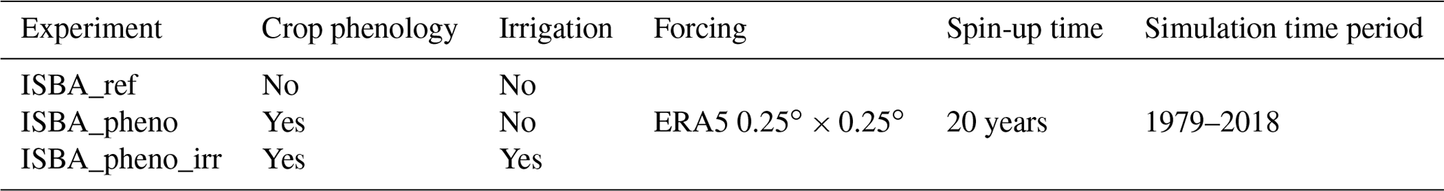
The SURFEX v8.1 version (Le Moigne et al., 2018) is used to do the simulations. Since this study focuses on irrigation, only the tile of natural and cultivated lands is simulated with ISBA, representing the evolution of soil (temperature and water profiles), vegetation (leaf-level and canopy-level photosynthesis, biomass, LAI, and carbon fluxes), surface hydrology (runoff and drainage), and snow conditions. To represent the global-scale diversity of continental natural surfaces, 20 different land surface types can be used in ECOCLIMAP-SG (see Fig. S1 and Table S2). The ISBA LSM simulations are made at a spatial resolution of 0.25∘ × 0.25∘ over a 40-year period from 1979 to 2018. The initial values of the soil moisture and soil temperature profiles are derived from a 20-year spin-up simulation by repeating year 1979. The same initial conditions are used for all the simulations, with and without crop phenology and irrigation modelling. All land surface types are grouped into 15 patches, including three irrigated ones, namely shrubs (orchards), C3 crops (typically wheat and rice), and C4 crops (corn). This study focuses on the results of these last two land surface types because there are hardly any irrigated orchards in Nebraska in the irrigation map described in Sect. 2.4.1. The dates of the irrigation season for corn are chosen in accordance with the literature (USDA and NASS, 2010) from May (emergence) to September (harvest), with a random picking of the day within those specific months. Three types of simulations are performed (Table 2), i.e. ISBA_ref, without irrigation or crop phenology (the benchmark), ISBA_pheno, with only crop phenology attributes (emergence and harvest dates), and the complete ISBA_pheno_irr simulation, with irrigation and crop phenology attributes. For the intercomparison of the simulations, we select areas where the irrigation fractional coverage is larger than 50 %, as determined from the irrigation map, in order to better assess the local effects of irrigation in offline simulations.
Table 2Main set-up of the three 40-year evaluation experiments driven by ERA5 atmospheric variables over Nebraska. Crop phenology is defined by emergence and harvest dates, while irrigation corresponds to additional water supply.
The reference ISBA_ref LAI simulations are compared with those from ISBA_pheno and ISBA_pheno_irr experiments and with the 0.01∘ × 0.01∘ LAI satellite observations over areas in Nebraska where the vegetation is considered to be C3 or C4 irrigated crops by ECOCLIMAP-SG. In addition to LAI, other variables are considered, including gross primary production (GPP) and land surface temperature (LST). In order to compare the time series simulations with observations, the Pearson correlation coefficient (r) and the root mean square difference (RMSD) scores are used. For water and carbon fluxes, they are calculated using daily values.
where y and x stand for observations and model simulations, respectively, and
are observation and model simulation means, respectively.
N represents the number of observations interpolated or aggregated to the considered model grid cell, which is used in the calculation of the scores.
The significance of r, r differences, and RMSD differences is tested using Fisher's test, Fisher's z test, and a paired sample Student's t test, respectively. Significance levels of 0.01, 0.05, and 0.05 are used to reject the null hypothesis of the tests, respectively.
2.4 Data
2.4.1 Irrigation map
One of the main challenges of this study is to obtain an upgraded map of irrigation at the global scale to be consistent with the resolution (300 m × 300 m) of the European Space Agency Climate Change Initiative (ESA-CCI) land cover map used in ECOCLIMAP-SG. The 1 km × 1 km resolution global irrigation map, proposed by Meier et al. (2018a) and based on a statistical approach and satellite data, is used. A reason to choose this product is that its development process is based (amongst other factors) on the ESA-CCI land cover product (v1.6.1), which is the same as the one used to develop the ECOCLIMAP-SG vegetation map (Sect. S1).
In order to transfer the Meier et al. (2018a) irrigation map (1 km × 1 km) to ECOCLIMAP-SG (300 m × 300 m), a spatial resampling of the Meier et al. (2018a) map is performed (https://doi.org/10.5281/zenodo.7221291; Druel, 2022). A simple majority rule is used by assigning, to each 300 m × 300 m grid point of ECOCLIMAP-SG, the irrigation status (irrigated or rainfed) of the main corresponding grid cell of the Meier et al. (2018a) 1 km × 1 km map. An irrigation map at a spatial resolution of 300 m × 300 m is obtained, with a single vegetation type attributed to each grid cell together with the irrigation status. The main limitation of this map is that there is no information on the type of irrigation. In this study, we consider that all irrigation is of sprinkler type, as this is the most common irrigation type in the USA and in Nebraska (AQUASTAT and FAO, 2019), where the test bed area of this study is located. This entails that irrigation water is added to the precipitation forcing over the irrigated agricultural parcels.
2.4.2 Atmospheric forcing
The simulations presented in this study are not coupled with the atmosphere. They are driven by a simulated atmospheric dataset of the European Centre for Medium-Range Weather Forecasts (ECMWF), which is the ERA5 atmospheric reanalysis at 0.25∘ × 0.25∘ (Hersbach et al., 2018, 2020). This global dataset was successfully used to force the ISBA LSM in previous studies (e.g. Albergel et al., 2019; Bonan et al., 2020). Beck et al. (2019) show that the ERA5 precipitation dataset is reasonably consistent with gauge–radar data over CONUS, except for mountainous areas. A subset of the ERA5 forcing over Nebraska is used for the time period from 1979 to 2018. This period is chosen in order to encompass various validation datasets. The following atmospheric variables are used to force the ISBA LSM and are taken from ERA5 at an hourly time step: air temperature, wind speed, air specific humidity, atmospheric pressure, shortwave and longwave downwelling radiation, and precipitation (liquid and solid).
2.4.3 Validation datasets
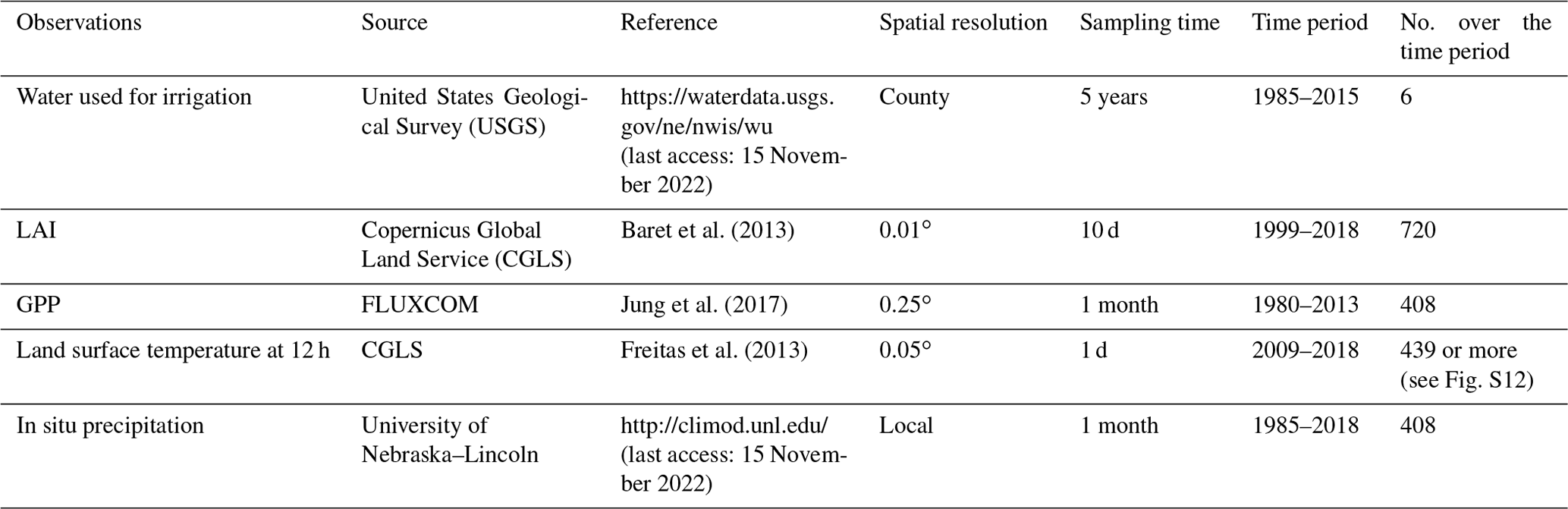
Five observation datasets are used (Table 3) to evaluate the simulations over Nebraska, namely the water used for irrigation, satellite-derived leaf area index (LAI), gross primary production (GPP), land surface temperature (LST), and precipitation.
Precipitation data from the Grand Island and Lincoln weather stations (40.96∘ N–98.31∘ W, 40.83∘ N–96.76∘ W; Gi dot in Fig. 2e and Li dot in Fig. 2b, respectively) are used to evaluate the ERA5 precipitation forcing over Nebraska. The two weather stations are within 170 km of each other and correspond to contrasting environmental conditions. While the Grand Island station is located within a densely irrigated area, the Lincoln station is located at Lincoln Airport, which is surrounded by rainfed agricultural fields.
The water use records are provided by the U.S. Geological Survey (USGS) through the National Water Information System (available at https://waterdata.usgs.gov/ne/nwis/wu, last access: 15 November 2022). Every 5 years, from 1985 onward, the annual raw amount of water collected for irrigation is available by county, together with conveyance loss and with the surface area of the irrigated vegetation. This allows us to compute the amount of water used for irrigation per unit surface area (mm) over the specific studied zone in Nebraska (Fig. 2e). The USGS data we use cover the 1985–2019 time period. Because conveyance loss data are not available for 1995, this year is not taken into account. In order to assess the consistency of the simulated irrigation process with observations, the simulated irrigation water amount on irrigated areas in Nebraska is compared with the USGS irrigation water amount estimates. Irrigation water amount is obtained from the simulated number of irrigation events using the model default irrigation water amount of 30 mm per irrigation event. Values of the mean and standard deviation of the yearly irrigation amount are compared. The comparison is made for the irrigated croplands (either C3 or C4 crops) as defined using the irrigation map (Sect. 2.4.1) within the studied irrigated area in Nebraska (Fig. 2e).
The simulated LAI is compared with a satellite-derived LAI product at 0.01∘ × 0.01∘ spatial resolution derived from SPOT-VGT and PROBA-V satellite data (up to May 2014 and after May 2014, respectively) by the European Copernicus Global Land Service (CGLS). This LAI product is described in Baret et al. (2013). We use version 2 of this product (GEOV2). It is available every 10 d from 1999 onward. It does not cover the whole simulation time period (1979 to 2018).
The simulated GPP is compared to an upscaled estimate of GPP available at 0.5∘ from 1980 to 2013, from the FLUXCOM project (Jung et al., 2017). Al-Yaari et al. (2021) show that the FLUXCOM daily evapotranspiration product can be used as a benchmark over irrigated areas. Since evapotranspiration and GPP fluxes are closely connected to each other, it can be assumed that the FLUXCOM GPP product is also sensitive to irrigation. The FLUXCOM product is based on a global machine learning model that does not have to be locally trained. However, it seems that three flux stations in Nebraska are used in the training, as their data are included in the La Thuile dataset used to build FLUXCOM (Tramontana et al., 2016). These stations are located at 45 km at the northeast of the Lincoln weather station (e.g. Suyker and Verma, 2009) in a region where irrigation is present but not dominant.
The simulated LST at 12:00 (local solar time) is compared to the LST derived from geostationary meteorological satellites by CGLS at 12:00 (local solar time). This product has a spatial resolution of 0.05∘ × 0.05∘ and is available from 2009 to 2018 (Freitas et al., 2013). It must be noticed that, in the version of the model used in this study, a single composite soil vegetation energy budget is used, and the thermal effect of crop residues is not represented. This means that, over croplands, the simulated LST can differ from the vegetation temperature as seen from space.
In addition to the validation datasets, corn LAI observations at the field scale for various agricultural management conditions are available in Boedhram et al. (2001).
The results presented below are focused on the impacts of the crop phenology and irrigation implementation on the simulated land surface variables over Nebraska. In addition to these results, illustrations of the response to irrigation of simulated key land surface variables (SWI, LAI, GPP, evapotranspiration, and LST) are shown over southwestern France and over the Hampton area in Nebraska in Sects. S2 and S3, respectively. In the case of Hampton, it can be noticed that the simulated irrigation mainly occurs in July and August (Fig. S7).
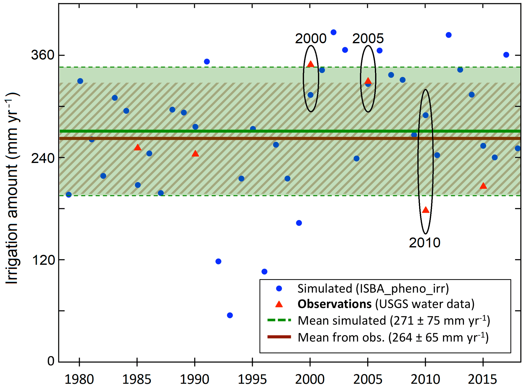
Figure 3Yearly cumulated irrigation amounts simulated by the model for the studied area in Nebraska from 1979 to 2018 (blue dots). The six USGS observations from 1985 to 2015 are shown (red triangles). The mean and standard deviation of the yearly values are shown for the model (green solid and dashed lines, respectively) and for the USGS data (brown lines). The 2000 and 2005 dry years are indicated, together with the 2010 wet year.
3.1 Irrigation: water use
In Fig. 3, the mean yearly irrigation amount for C3 and C4 crops for the ISBA_pheno_irr experiment is compared to the values derived from the observations from the USGS. The simulated irrigation amount presents a large interannual variability, with a minimum of 60 mm in 1993 and a maximum close to 390 mm in 2002. It must be noted that 1993 is one of the wettest year recorded at the Lincoln weather station (https://lincolnweather.unl.edu/records/annual.asp, last access: 15 November 2022). The mean simulated value of the yearly irrigation water amount used for irrigation (271±75 mm yr−1) slightly overestimates the observed one (264±65 mm yr−1), with a difference of +2.7 %. This difference could be explained by the availability of the water resource, which is not explicitly accounted for by the model yet. The large observed irrigation amounts in 2000 and 2005, larger than 300 mm yr−1, are relatively well represented by the model. On the other hand, the observed small irrigation amount for the 2010 wet year is overestimated by about 110 mm yr−1. In situ precipitation observations over Grand Island indicate that year 2010 is wetter than 2005 and 2000 during the growing season, with 575, 508, and 277 mm from May to September, respectively. In 2010, the ERA5 precipitation bias from July to September triggers a cumulated precipitation gap of 103 mm (Fig. S18a). The model responds to this water deficit by triggering irrigation at the end of the growing season, especially in August (Fig. S18c). On the other hand, ERA5 is unbiased at the beginning of the growing period (May–June 2010).
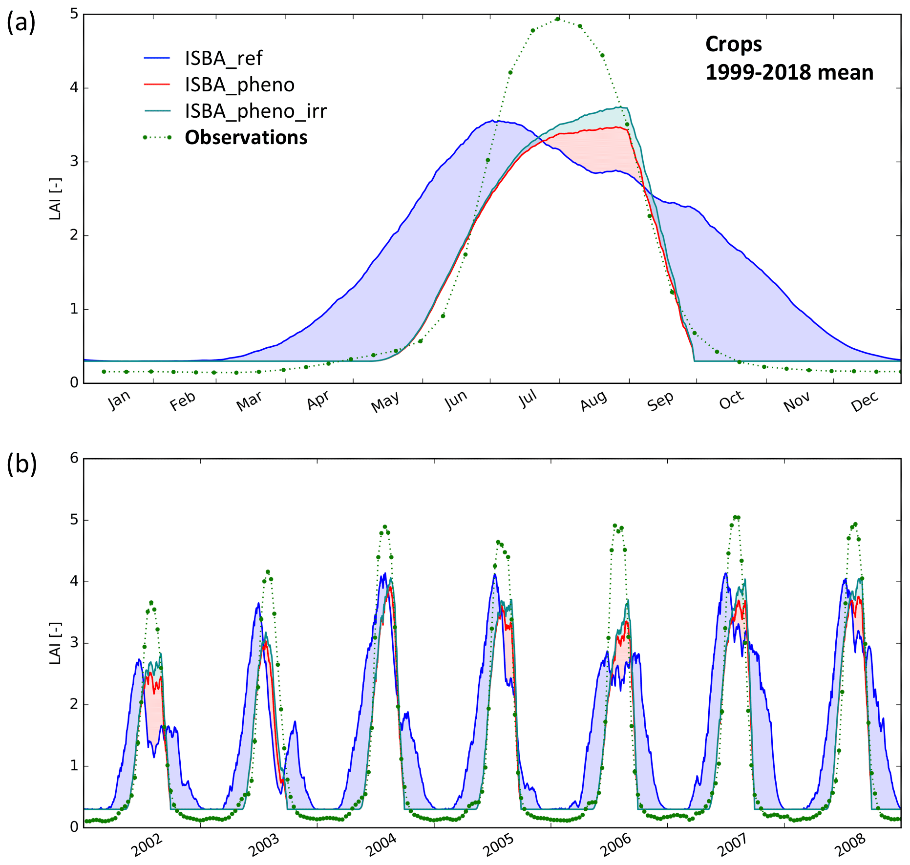
Figure 4LAI (m2 m−2) of irrigated crops (C3 or C4) in the most densely irrigated part of Nebraska (Fig. 2e). (a) Seasonal variation for the time period from 1999 to 2018. (b) Daily time series from 2002 to 2008. Simulated LAI is shown for the irrigated fraction, from the reference simulation (ISBA_ref, blue line), and from the simulations with only agricultural practices and with agricultural practices and irrigation (ISBA_pheno, red line, and ISBA_pheno_irr, cyan line, respectively). Satellite-derived LAI observations (green dots) are for areas where the fraction of C3 or C4 irrigated crops is larger than 50 %.
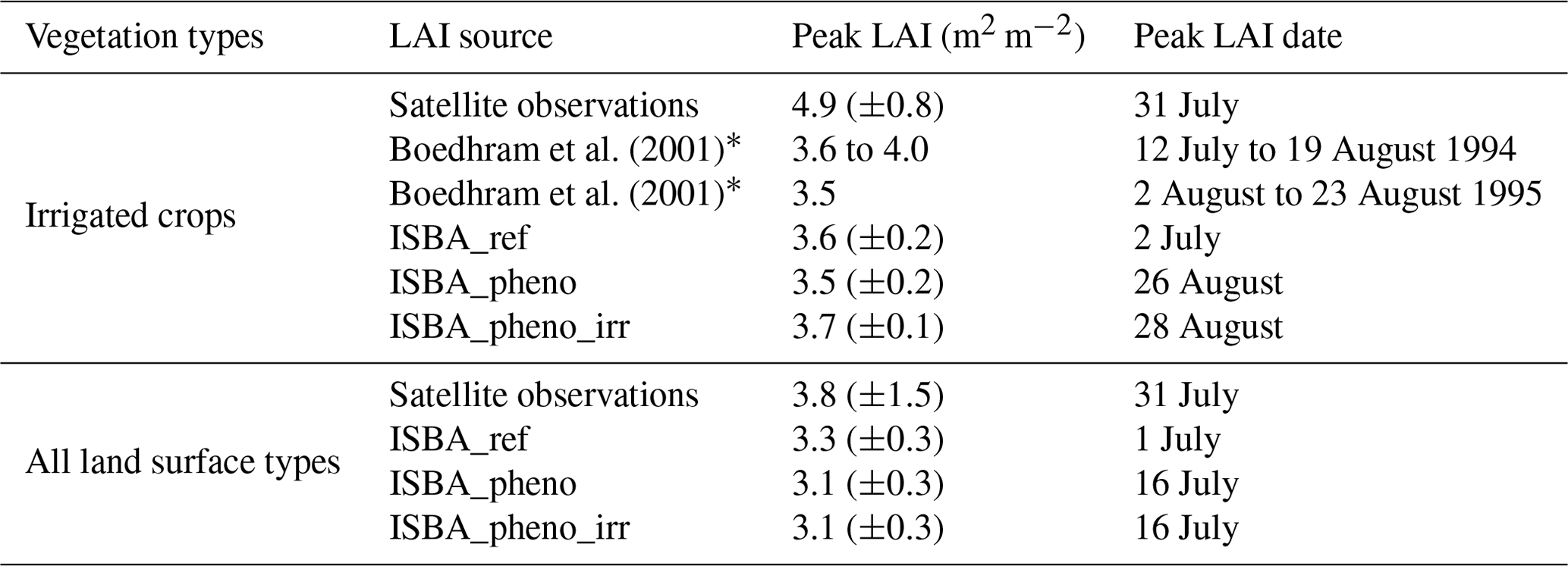
Table 4Observed and simulated mean LAI peak characteristics over Nebraska for the 1999–2018 time period for irrigated crops (see Fig. 4) and all land surface types (see Fig. 5).
* Boedhram et al. (2001) data are for fertilised irrigated corn in 1994 and 1995.
3.2 Irrigation: plant growth
Figure 4 illustrates the mean seasonal and interannual variability in LAI of irrigated crops (either C3 or C4) in the most densely irrigated part of Nebraska for areas with a fraction of irrigated crops larger than 50 % in Fig. 2e, from 1999 to 2018. Table 4 presents the peak LAI characteristics. While the satellite LAI observations present a peak at the end of July, the modelled LAI is plateauing in August (Fig. 4). Figure 2 in Boedhram et al. (2001) shows that the modelled LAI plateau in August at LAI values of about 3.7 m2 m−2 is realistic for irrigated corn. The satellite LAI observations are sensitive to both rainfed and irrigated vegetation. A comparison across all vegetation types is presented in Sect. 3.3. In all ISBA LAI simulations, the start of the growing season corresponds to a gradual increase in LAI from the initial value of LAI = 0.30 m2 m−2 imposed to the model in winter. The observed LAI presents a smaller, minimum LAI value of 0.15 m2 m−2, which starts increasing in April, and a value of 0.30 m2 m−2 is reached at the end of April. Then, plant growth continues at about the same low rate till the end of May. The LAI growth rate increases in June and LAI reaches a mean peak value of 4.9 (±0.8) m2 m−2 on 31 July (Table 4). The observed LAI then sharply decreases to reach its minimum value at about the end of September.
The ISBA_ref LAI simulations do not mirror the observed late growing season and rapid senescence. The ISBA_ref vs. observations comparison shows that, without crop phenology and without irrigation, the simulated LAI generally starts increasing in March. On average, a peak LAI value of 3.6 (±0.2) m2 m−2 is simulated by ISBA_ref on 2 July, before slowly decreasing until the end of December. The ISBA_ref growing season is much longer than observed. It starts 2 months before the observations and stops 3 months after the observations. The simulated LAI peaks 1 month before the observations. The simulated yearly LAI amplitude is 28 % smaller than observed.
The ISBA_pheno LAI simulation is much more consistent with the LAI observations. The growing season starts in mid-May, and the senescence ends at the end of September. However, the simulated peak LAI is still 30 % smaller than observed (LAI = 3.5 (±0.2) m2 m−2). The peak LAI is reached on 26 August, much later that the ISBA_ref peak LAI, and about 1 month after the observed peak. The sharp decrease in LAI in September results from harvests at random dates in September. Adding irrigation (ISBA_pheno_irr) does not change the general pattern of the LAI curve but increases the LAI amplitude, with a mean peak LAI value of 3.7 (±0.1) m2 m−2 on 28 August, which is larger (+8 %) than for ISBA_pheno but still below the observation (−24 %).
The interannual variability in simulated and observed LAI values is illustrated in Fig. 4b, from 2002 to 2008. The ISBA_ref LAI presents a systematic drop in summer, which is neither present in the observations nor simulated by the ISBA_pheno and ISBA_pheno_irr experiments. Without the regular seasonality imposed by crop phenology parameters, the model may simulate a regrowth of vegetation in autumn (e.g. in 2003) that is not present in the observations. The ISBA_pheno and ISBA_pheno_irr simulations are more consistent with the observed seasonality.
3.3 Impact of crop phenology and irrigation on LAI at a regional scale
This section is focused on the impact of irrigation practices for the southern Nebraska zone (as defined in Fig. 2e), and all land surface types are considered for the comparison with observations at a spatial resolution of 0.25∘ × 0.25∘.
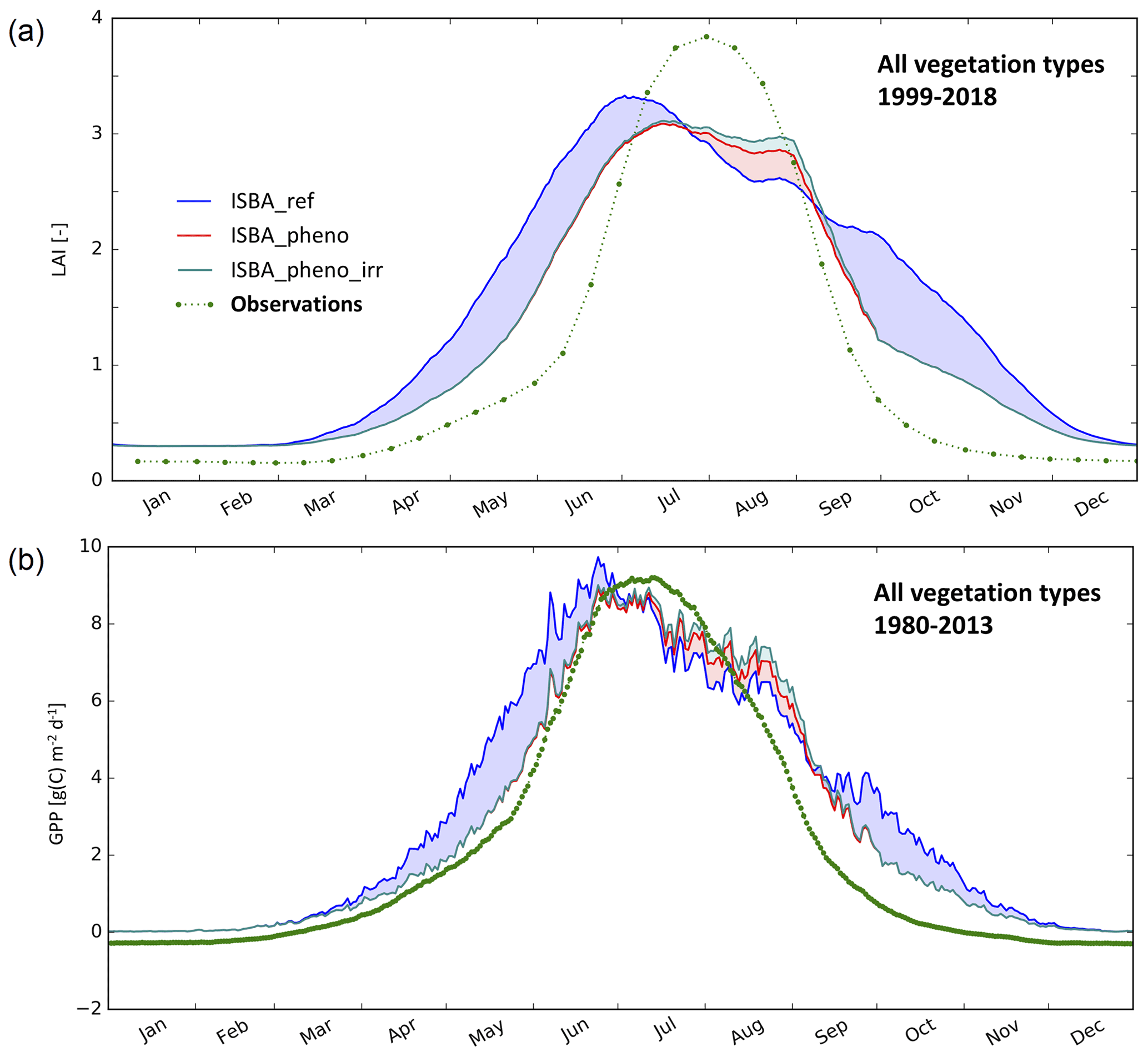
Figure 5Simulated vs. observed LAI and GPP of all vegetation types in the most densely irrigated part of Nebraska (Fig. 2e). (a) Seasonal variation in mean LAI (m2 m−2) from 1999 to 2018. (b) Seasonal variation in mean GPP (g C m−2 d−1) 1980 to 2013. ISBA_ref, ISBA_pheno, and ISBA_pheno_irr simulations are represented by blue, red, and cyan lines and satellite-derived observations by green dots.
Figure 5a shows the seasonal mean LAI variations from 1999 to 2018. This figure is similar to Fig. 4a, but all land surface types are considered. Peak LAI characteristics are given in Table 4. They differ from the irrigated crop LAI peaks. While the observed LAI peaks at 3.8 (±1.5) m2 m−2 on 31 July, LAI peaks at 3.3 (±0.3) m2 m−2 on 1 July for ISBA_ref, 3.1 (±0.3) m2 m−2 on 16 July for ISBA_pheno, and 3.1 (±0.3) m2 m−2 on 16 July for ISBA_pheno_irr. Compared to irrigated crop simulations, the experiments with crop phenology (ISBA_pheno and ISBA_pheno_irr) present earlier peak LAI dates because they include rainfed crops and natural vegetation. Emergence dates are not imposed on rainfed crops and natural vegetation. This allows earlier leaf onset. The irrigated crop signature is visible in the second peak of the annual LAI cycle simulated by ISBA_pheno and ISBA_pheno_irr experiments at the end of August. More often than not (83 % and 88 % of the grid cells for r and RMSD, respectively), the LAI score differences between ISBA_pheno_irr and ISBA_ref shown in Fig. 6 correspond to an improvement in the LAI simulation with the representation of irrigation. A month-by-month analysis of the scores (Fig. 7) shows a significant improvement in r values in June and September. The r value can be increased by 30 %. Lower RMSD values are observed from April to November but more frequently in May and in October. In July, RMSD differences are not significant. In April, October, and November, the main cause of the reduction in RMSD values is the imposed minimum value of 0.3 m2 m−2 before the emergence (in May) and the harvest (in September). The ISBA_pheno correlation and RMSD differences with respect to ISBA_ref are nearly identical to those shown for ISBA_pheno_irr in Figs. 6–7 (not shown).
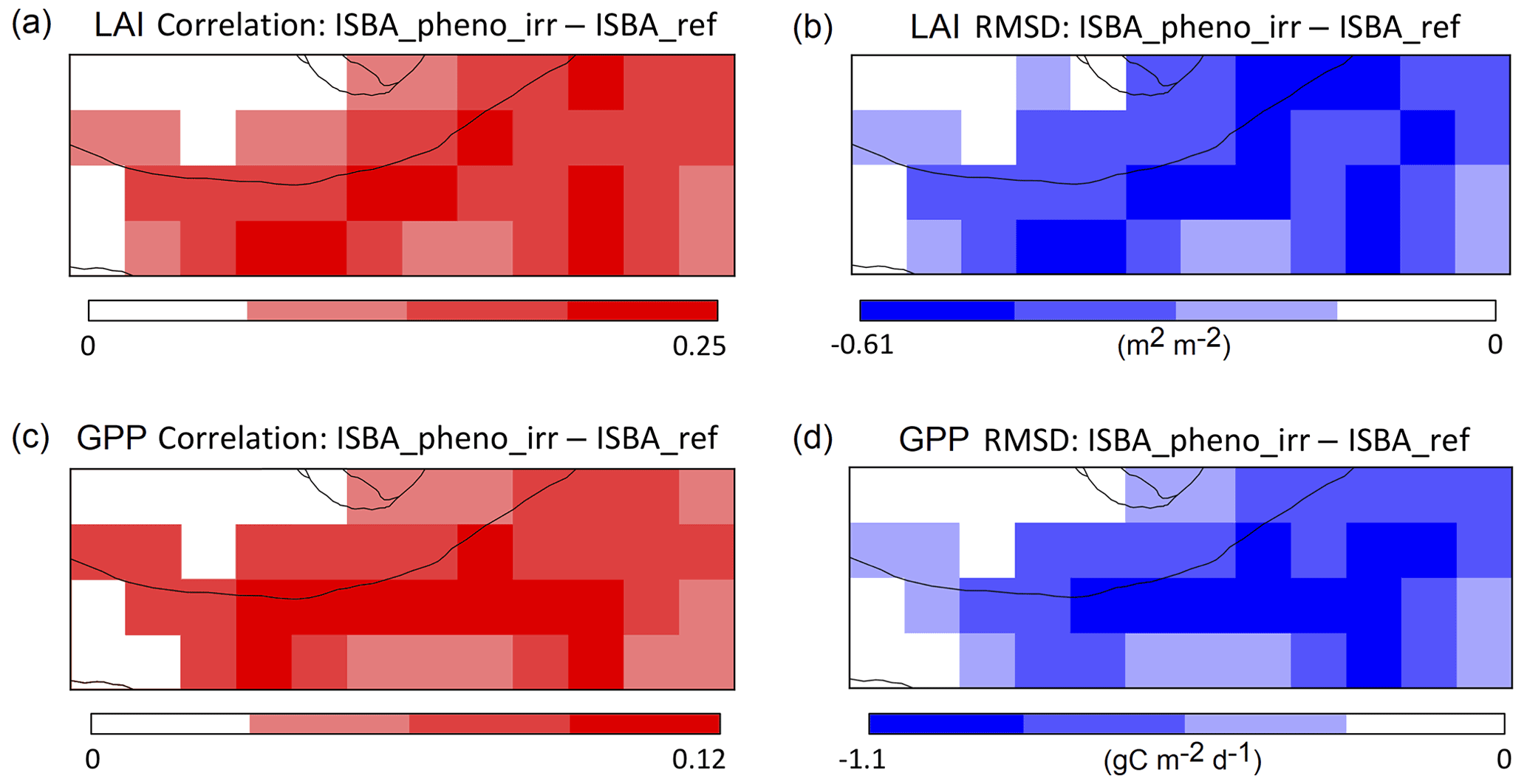
Figure 6Simulated vs. observed LAI and GPP of all vegetation types in the most densely irrigated part of Nebraska (Fig. 2e). (a, c) Temporal correlation and (b, d) RMSD score difference maps of (a, b) LAI and (c, d) GPP. White is used to mask the non-significant score difference values.
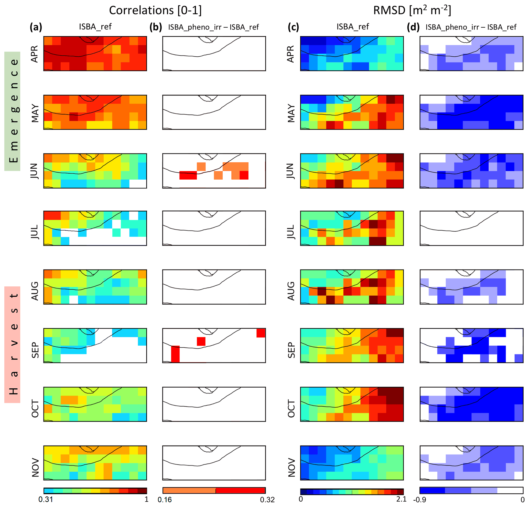
Figure 7Comparison of simulated LAI with CGLS LAI observations in the most densely irrigated part of Nebraska (Fig. 2e) from 1999 to 2018 during the vegetation growing and senescence time period from April to November. Monthly temporal correlation (a, b) and RMSD (c, d) maps are shown for the reference simulation without a representation of irrigation ISBA_ref (a, c). The added value of the ISBA_pheno_irr simulation with respect to ISBA_ref is shown through score difference maps (b, d). White is used to mask non-significant correlation and score difference values.
3.4 Impact on the GPP flux
As the vegetation productivity is linked to LAI, the seasonality pattern of GPP (Fig. 5b) is comparable to the one of LAI (Fig. 5a), but the observed GPP peak (9.2±2.1 g [C] m−2 d−1) occurs in mid-July while the observed LAI peaks on 31 July. During the plant growth period, the smallest differences between all the simulations and the observations occur at about the same time as the observed GPP peak. For all simulations, a GPP plateau with a value of 9.0±1.8 g [C] m−2 d−1 is reached at the beginning of July and lasts until mid-July. Finally, the simulated GPP decreases in September with a delay of about 2 weeks with respect to the observations.
Before July, the ISBA_ref photosynthetic activity is well in advance, as compared to the observations, of about 20 d in May. This is consistent with the very large LAI values simulated by ISBA_ref in May, with about 2 m2 m−2, while the mean LAI observation hardly exceeds 0.5 m2 m−2. The simulated GPP maximum (9.7±2.0 g [C] m−2 d−1) is reached before the end of June. After a sharp decrease at the end of June, the ISBA_ref GPP decreases at a slower rate than the observations. From mid-September to the end of October, the simulated GPP is much larger than the observed GPP.
The ISBA_ref flaws are much less pronounced in ISBA_pheno and ISBA_pheno_irr experiments. In the latter simulations, the increase in the GPP occurs at about the same time as in the observations. The GPP values are systematically larger with irrigation in July and August than for other simulations. As for LAI, the GPP, r, and RMSD scores (Fig. 6c and d, respectively) are better for ISBA_pheno_irr than for ISBA_ref, with an improvement of 87 % and 81 % over the domain, respectively.
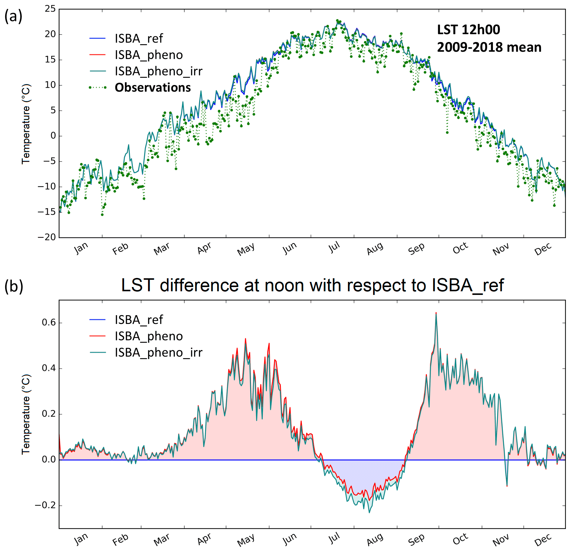
Figure 8Seasonal variation in surface temperature daily values at 12:00 local solar time (∘C) in the most densely irrigated part of Nebraska (Fig. 2e) from 2009 to 2018 (a), as derived from the reference simulation ISBA_ref (blue line), ISBA_pheno (red line), ISBA_pheno_irr (cyan), and the CGLS product (green dotted line). The surface temperature differences at 12:00 local solar time (b) of ISBA_pheno_irr and ISBA_pheno simulations with respect to the ISBA_ref simulations are shown.
3.5 Impact on LST
In order to evaluate the impact of irrigation on the land surface energy budget, Fig. 8 shows the land surface temperature at 12:00 local solar time simulated by the three model configurations and derived from the CGLS product. Overall, ISBA tends to overestimate the LST at noon, especially in April–May, by up to 7 ∘C (Fig. 8a). The bias is reduced during the summer.
Due to the difficulty of observing the differences between the simulations, Fig. 8b presents differences in ISBA_pheno and ISBA_pheno_irr vs. ISBA_ref. With crop phenology (with or without irrigation), the simulated LST is globally higher from April to June and from mid-September to November. The maximum difference with respect to ISBA_ref is ∘C. It is observed for ISBA_pheno in September. During the summer (July and August), the new model versions tend to present lower LST values with temperature differences close to ∘C in ISBA_pheno_irr. Moreover, from May to mid-September, the temperature in ISBA_pheno_irr is lower than in ISBA_pheno, and this difference can reach −0.9 ∘C locally in summer.
The results presented in Sect. 3 show that the new version of ISBA is able to produce a realistic mean yearly irrigation water amount (Fig. 3). It also markedly improves the LAI and GPP simulations (Figs. 4, 5, and 6, respectively). On the other hand, it has a limited impact on the LST simulations and is not able to significantly reduce the strong model biases that are observed for this variable before and after the irrigation time period (Fig. 8).
4.1 Could the new crop phenology and irrigation scheme be further improved?
The crop phenology model is very simple, and adding more parameters related to phenology could be a way to further improve the model performance. Integrating satellite LAI observations in ISBA, using sequential data assimilation, is also an option (Mucia et al., 2020). The results of our numerical experiments over Nebraska show that considering crop phenology improves the consistency of the simulations with LAI and GPP observations. The corresponding correlation and RMSD scores are improved. The crop phenology parameters used to force emergence and harvest dates reduce the length of the growing season, delay spring growth, and avoid a regrowth in the autumn. It seems that irrigation only plays an additive role in improving the vegetation seasonal cycle as compared to the role of including crop phenology (Sect. 3.3). Both crop phenology and irrigation models have shortcomings, and their performance is limited by difficulties in simulating processes that are not directly related to irrigation.
First, the same emergence and harvest dates are imposed for all years, while in reality crop phenology may present an interannual variability related to climate conditions. This is particularly the case for Nebraska because the start of the growing season depends on the snowmelt and soil thawing dates. These processes are represented in ISBA and crop phenology parameters could be related to snow melting and soil thawing, but this would require extensive developments to be implemented on a global scale. Moreover, the representation of the cold season processes is not perfect in ISBA (Decharme et al., 2019), and the model tends to underestimate snow depth and the length of the snow season. This could explain biases in soil temperature and LST simulations before and after the irrigation time period. Figure 8 shows that LST values below the freezing level can be observed in April, and that their model counterparts are about 7 ∘C warmer. The earlier thawing in model simulations is reflected in the much earlier leaf onset in LAI simulations. Figure 5 shows that, while the observed LAI does not exceed 0.5 m2 m−2 at the end of April, the ISBA_ref LAI reaches the same value about 1 month earlier. The unrealistically early leaf onset is consistent with the warm model bias at the end of the cold season. This shows that improving the representation of the cold season by assimilating satellite-derived or in situ snow cover fraction observations could improve the simulation of the crop growing period in this area. Also, emergence and harvest dates could be derived from the LAI observation in order to better represent the interannual variation. However, the currently used random approach to establish the crop season provides robust results over the irrigated grid cells (Fig. 4).
Second, the irrigation itself is based on fixed parameter values such as the minimum period between two consecutive irrigations (1 week) and SWI levels triggering irrigation events. The simulations over the Hampton grid cell show that the first irrigation can start at quite low levels of the SWI (Fig. S7), even below the second irrigation threshold of 0.55 defined in Sect. 2.2. Suppressing the 1-week constraint of irrigation events improves the simulation of the peak LAI, which otherwise is rather poorly simulated (Fig. 4). However, this change triggers unrealistic large irrigation water amounts (not shown). A lack of irrigation water amount cannot explain the excessive soil water deficit. A possible explanation could be that the initial soil water storage value between the end of the cold season and the first irrigation event is withdrawn too quickly from the soil by the model. One could also challenge the quality of the ERA5 precipitation. ERA5 precipitation compares rather well with in situ observations, and the seasonal and interannual variability is fairly represented (Figs. S13 and S14). The comparison with in situ precipitation observations at the Grand Island station shows that ERA5 tends to markedly overestimate precipitation in April by 0.57 mm d−1, i.e. 27 % on average from 1985 to 2018 (Fig. S15). This is rather systematic, i.e. 8 years out of 10 (Fig. S16). In July, ERA5 precipitation can be much smaller than the observations, for example, in 1991 and 2007 (Fig. S17).
A possible limitation of using a global low-resolution reanalysis such as ERA5 is that changes to the local climatic conditions caused by irrigation may not be represented. Over Nebraska, Szilagyi and Franz (2020) show that the decadal increase in irrigated land tends to trigger a reduction in precipitation over the most densely irrigated areas of about −10 mm per decade. The largest precipitation suppression is observed in spring, in March, before the corn growing season, in relation to larger soil water content values. In our simulations, ISBA_pheno_irr presents larger soil moisture values than ISBA_ref in March (see Fig. S7), but this is mainly due to crop phenology. The ERA5 screen-level 2 m air temperature and relative humidity are analysed together with soil moisture by assimilating in situ observations from ground weather stations (Hersbach et al., 2020). In large irrigated areas where weather stations are present, the assimilation should be able to represent the soil moisture effect on these variables, even at coarse spatial resolution. A large-scale experiment involving ground and airborne measurements was recently performed in northeastern Spain to assess the impact of irrigation on atmospheric model simulations (Boone et al., 2021). In this context, high-resolution atmospheric data from the Application of Research at the Operational Mesoscale (AROME) numerical weather forecast model are available to drive the ISBA model. AROME is run operationally at 1.3 km over western Europe. Future developments will focus on the intercomparison of ISBA simulations at various spatial resolutions and under different conditions, as the choice of spatial resolution may affect the simulation of the smaller irrigation variabilities.
4.2 Are evaporation components simulated well?
All evaporation terms (plant transpiration, soil evaporation, and interception) are simulated by ISBA. Under given environmental conditions, the simulated plant transpiration is not proportional to LAI. A simple canopy radiative transfer model is used to simulate the available photosynthetically active radiation (PAR) within the vegetation canopy. The response of GPP and transpiration to PAR and to LAI is controlled by this radiative transfer model. Photosynthesis and transpiration are calculated for three layers and summed to calculate canopy-level values. For large LAI values, the mean leaf-level GPP and transpiration simulations are reduced in relation to smaller vegetation transmittance to solar radiation. The impact of changes in LAI on mean leaf-level GPP and transpiration is large at intermediate LAI values ranging from 1 to 3 m2 m−2. It is much reduced for LAI values larger than 3 m2 m−2. An improved version of this radiative transfer model able to represent 10 canopy layers, and a more realistic response to solar zenith angle will be available in the next version of SURFEX (Delire et al., 2020). Over the Hampton irrigated area, total evapotranspiration of ISBA_ref and ISBA_pheno_irr is quite similar (Fig. S9). On the other hand, soil evaporation and plant transpiration differ. In the ISBA_pheno_irr simulation, transpiration is reduced in spring by more than 30 % compared to ISBA_ref. The lower transpiration is offset by larger soil evaporation values (Fig. S9c). As a result, total evapotranspiration does not change much. Also, the new crop phenology and irrigation module does not affect interception much (Fig. S10). The soil evaporation component could be overestimated because (1) the soil is too warm in relation to a poor representation of thawing or because (2) crop residues at the soil surface are not represented. Wortmann et al. (2012) show that, in this area, not harvesting crop residues tends to reduce soil evaporation and increase crop yield, limit water runoff, soil erosion, and contributes to maintaining soil fertility. Suyker and Verma (2009) show that increasing surface mulch dry mass from 50 to 150 g m−2 can decrease the non-growing season evapotranspiration by more than 20 %. The ISBA model includes a representation of litter in forests (Napoly et al., 2017) that will be generalised to low vegetation in the next version of SURFEX. Using this new capability could improve our simulations.
The use of independent evapotranspiration datasets is investigated in Sect. S3. In particular, in situ observations over an irrigated corn field (Suyker and Verma, 2009) are used. During the non-growing season, the ISBA_pheno_irr model overestimates evapotranspiration by 48 % (Table S4). The ISBA_pheno_irr evapotranspiration peak (in June) tends to happen too early (Table S5; Fig. S11). This bias in spring could be caused by too large soil evaporation values. Mean values of near-surface wind speed are particularly large over Nebraska, especially during wintertime and springtime (Chen, 2020). This feature could exacerbate the impact of a misrepresentation of soil evaporation.
4.3 Is the irrigation scheme flexible enough?
In this study, sprinkler irrigation is considered. The model is able to represent other irrigation systems such as flooding irrigation but more developments are needed to limit the runoff to the irrigated plot, and this options needs to be validated. The newly implemented irrigation processes, along with the new ECOCLIMAP-SG vegetation description, let users choose which land surface type should be irrigated. Irrigation can be represented at various spatial scales, ranging from the field scale for agricultural studies to the global scale for climate studies. Model parameters can be specified using new datasets or local characteristics. For example, in this article we use a unique date for starting and ending the crop growing season with a random variability, but more accurate dates can be prescribed (varying spatially and from one vegetation type to another or using crop calendars). Moreover, the better spatial resolution of ECOCLIMAP-SG allows the use of high-resolution atmospheric forcing. This provides new opportunities for assessing the impact of irrigation on local climate and water resource conditions.
This study is mainly focused on a zone in the south of Nebraska where the irrigation density is relatively high (Fig. 2), and results could differ in other regions. Except for the fixed emergence and harvesting dates corresponding to regional crop phenology (from USDA and NASS, 2010), default values are used for all the other parameters (Sect. 2.4). Tests performed in southwestern France (Sect. S2) allow us to ensure that the model is able to work in contrasting climate conditions.
In this study, the ISBA simulations are neither coupled to the atmosphere nor to the CTRIP river routing system. Such coupled numerical experiments can be performed thanks to the SURFEX modelling platform. However, more developments are needed in order to ensure water conservation in the hydrological system. In particular, irrigation water amounts should be consistent with the available water resource in rivers, groundwater, and dams.
A new uncalibrated crop phenology and irrigation scheme able to work on a global scale is implemented within the ISBA land surface model in order to improve the representation of vegetation over agricultural areas. A case study over an irrigated area in the state of Nebraska (USA) is performed to validate the new scheme. Simple crop phenology rules represent emergence and harvesting and improve the seasonality of plant growth, while the additional water supply from the irrigation mostly impacts the peak LAI value. The model is able to produce a realistic yearly irrigation water amount and markedly improves the LAI and GPP. It is shown that model performance can be limited by processes not directly related to irrigation, such as thawing or crop residues. The irrigation scheme has many possible configurations, and the code is highly flexible. With this capability, ancillary data on farming practices, such as emergence and harvest dates or the amount of water per irrigation event, can be used. This flexible crop phenology and irrigation scheme can take the spatial heterogeneity of irrigation activities into account and detect irrigation-induced impacts on Earth system simulations. Our results show that crop phenology parameters modify the seasonal pattern of the simulation of LAI, soil moisture, evapotranspiration, and plant carbon uptake and that irrigation affects their magnitude. This provides the basis for further development in offline and online applications of the ISBA model.
SURFEX can be downloaded freely at http://www.umr-cnrm.fr/surfex/data/OPEN-SURFEX/open_surfex_v8_1_20210914.tar.gz (last access: 15 November 2022; CNRM, 2016). It is provided under a CECILL-C License (French equivalent to the L-GPL licence). The version developed and used for the experiment in this study is available at https://doi.org/10.5281/zenodo.5718063 (Druel, 2021). It based on the SURFEX version 8.1 (ref f70f6457). For future use, it is strongly recommended to use the newest version of ISBA within the SURFEX version 9.0 (scheduled for release in 2022) in which the irrigation model will be included by default.
Global irrigation data are available from https://doi.org/10.1594/PANGAEA.884744, (Meier et al., 2018b), ERA5 data from https://doi.org/10.24381/cds.adbb2d47 (Hersbach et al., 2018), USGS water use data for Nebraska from https://waterdata.usgs.gov/ne/nwis/wu (last access: 15 November 2022; USGS, 2018), CGLS LAI data from https://land.copernicus.vgt.vito.be/PDF/portal/Application.html#Browse;Root=512260;Collection=1000083;Time=NORMAL,NORMAL,-1,,,-1,, (last access: 15 November 2022; Copernicus, 2020), GPP from https://www.fluxcom.org/, last access: 15 November 2022; FluxCom, 2020), CGLS hourly LST data from https://land.copernicus.vgt.vito.be/PDF/portal/Application.html#Browse;Root=520752;Collection=1000300;Time=NORMAL,NORMAL,-1,,,-1,, (last access: 15 November 2022; Copernicus, 2019). Initialisation files are available at https://doi.org/10.5281/zenodo.7221291 (Druel, 2022).
The supplement related to this article is available online at: https://doi.org/10.5194/gmd-15-8453-2022-supplement.
AD and CA designed the experiments. AD carried out the implementation of the irrigation scheme and performed the simulations. AD wrote the paper. Both co-authors participated in the analysis of the results and the revision of the paper.
The contact author has declared that none of the authors has any competing interests.
Publisher's note: Copernicus Publications remains neutral with regard to jurisdictional claims in published maps and institutional affiliations.
The work presented here has been supported by the project URCLIM (advancement of URban CLIMate services, part of ERA4CS, an ERA-NET initialised by JPI Climate with co-funding of the European Union; grant no. 690462). The authors would like to thanks Stephanie Faroux and Marie Minvielle, in charge of the SURFEX code support, for technical assistance, Deborah Verfaillie, for her careful reading of the paper, and Jinkyu Hong, Fabian Stenzel, and the anonymous reviewers, for their helpful comments.
This research has been supported by the H2020 Environment (grant no. 690462).
This paper was edited by Jinkyu Hong and reviewed by Fabian Stenzel and four anonymous referees.
Adegoke, J. O., Pielke, R. A., Eastman, J., Mahmood, R., and Hubbard, K. G.: Impact of Irrigation on Midsummer Surface Fluxes and Temperature under Dry Synoptic Conditions: A Regional Atmospheric Model Study of the U.S. High Plains, Mon. Weather Rev., 131, 556–564, https://doi.org/10.1175/1520-0493(2003)131<0556:IOIOMS>2.0.CO;2, 2003.
Albergel, C., Dutra, E., Bonan, B., Zheng, Y., Munier, S., Balsamo, G., de Rosnay, P., Munoz-Sabater, J., and Calvet, J.-C.: Monitoring and forecasting the impact of the 2018 summer heatwave on vegetation, Remote Sens., 11, 520, https://doi.org/10.3390/rs11050520, 2019.
Al-Yaari, A., Ducharne, A., Tafasca, S., Mizuochi, H., and Cheruy, F.: Influence of irrigation on the bias between ORCHIDEE and FLUXCOM evapotranspiration products, 2021 IEEE International Geoscience and Remote Sensing Symposium IGARSS, 6552–6555, https://doi.org/10.1109/IGARSS47720.2021.9554734, 2021.
AQUASTAT and FAO: Country Fact Sheet, United States of America, http://www.fao.org/nr/water/aquastat/data/cf/readPdf.html?f=USA-CF_eng.pdf (last access: 15 November 2022), 2019.
Baret, F., Weiss, M., Lacaze, R., Camacho, F., Makhmara, H., Pacholcyzk, P., and Smets, B.: GEOV1: LAI and FAPAR essential climate variables and FCOVER global time series capitalizing over existing products. Part1: Principles of development and production, Remote Sens. Environ., 137, 299–309, https://doi.org/10.1016/j.rse.2012.12.027, 2013.
Beck, H. E., Pan, M., Roy, T., Weedon, G. P., Pappenberger, F., van Dijk, A. I. J. M., Huffman, G. J., Adler, R. F., and Wood, E. F.: Daily evaluation of 26 precipitation datasets using Stage-IV gauge-radar data for the CONUS, Hydrol. Earth Syst. Sci., 23, 207–224, https://doi.org/10.5194/hess-23-207-2019, 2019.
Biemans, H., Haddeland, I., Kabat, P., Ludwig, F., Hutjes, R. W. A., Heinke, J., von Bloh, W., and Gerten, D.: Impact of reservoirs on river discharge and irrigation water supply during the 20th century, Water Resour. Res., 47, W03509, https://doi.org/10.1029/2009WR008929, 2011.
Boedhram, N., Arkebauer, T. J., and Batchelor, W. D.: Season-long characterization of vertical distribution of leaf area in corn, Agron. J., 93, 1235–1242, https://doi.org/10.2134/agronj2001.1235, 2001.
Bonan, B., Albergel, C., Zheng, Y., Barbu, A. L., Fairbairn, D., Munier, S., and Calvet, J.-C.: An ensemble square root filter for the joint assimilation of surface soil moisture and leaf area index within the Land Data Assimilation System LDAS-Monde: application over the Euro-Mediterranean region, Hydrol. Earth Syst. Sci., 24, 325–347, https://doi.org/10.5194/hess-24-325-2020, 2020.
Bonnemort, C., Bouthier, A., Deumier, J.-M., and Specty, R.: Conduire l'irrigation avec Irritel ; intérêts et limites, La Météorologie, 14, 36–43, https://doi.org/10.4267/2042/51182, 1996.
Boone, A., Bellvert, J., Best, M., Brooke, J., Canut-Rocafort, G., Cuxart, J., Hartogensis, O., Le Moigne, P., Miró, J. R., Polcher, J., Price, J., Quintana Seguí, P., and Wooster, M.: Updates on the international Land Surface Interactions with the Atmosphere over the Iberian Semi-Arid Environment (LIAISE) Field Campaign, GEWEX News, 31, 16–21, 2021.
Bruinsma, J.: The resource outlook to 2050: By how much do land, water use and crop yields need to Increase by 2050?, FAO Expert meeting on How to Feed the World in 2050, 24–26 June 2009, Rome, Italy, https://www.fsnnetwork.org/sites/default/files/the_resource_outlook_to_2050by_how_much_do_land_water_and_crop_yields_need_to_increase_by_2050_.pdf (last access: November 2022), 2009.
Calvet, J.-C. and Champeaux J.-L.: L'apport de la télédétection spatiale à la modélisation des surfaces continentales, La Météorologie, 108, 52–58, https://doi.org/10.37053/lameteorologie-2020-0016, 2020.
Calvet, J.-C., Noilhan, J., Roujean, J.-L., Bessemoulin, P., Cabelguenne, M., Olioso, A., and Wigneron, J.-P.: An interactive vegetation SVAT model tested against data from six contrasting sites, Agric. For. Meteorol., 92, 73–95, https://doi.org/10.1016/S0168-1923(98)00091-4, 1998.
Calvet, J.-C., Gibelin, A.-L., Roujean, J.-L., Martin, E., Le Moigne, P., Douville, H., and Noilhan, J.: Past and future scenarios of the effect of carbon dioxide on plant growth and transpiration for three vegetation types of southwestern France, Atmos. Chem. Phys., 8, 397–406, https://doi.org/10.5194/acp-8-397-2008, 2008.
Carrillo-Guerrero, Y., Glenn, E. P., and Hinojosa-Huerta, O.: Water budget for agricultural and aquatic ecosystems in the delta of the Colorado River, Mexico: Implications for obtaining water for the environment, Ecol. Eng., 59, 41–51, https://doi.org/10.1016/j.ecoleng.2013.04.047, 2013.
Chen, L.: Impacts of climate change on wind resources over North America based on NA-CORDEX, Renewable Energy, 153, 1428–1438, https://doi.org/10.1016/j.renene.2020.02.090, 2020.
Chukalla, A. D., Krol, M. S., and Hoekstra, A. Y.: Green and blue water footprint reduction in irrigated agriculture: effect of irrigation techniques, irrigation strategies and mulching, Hydrol. Earth Syst. Sci., 19, 4877–4891, https://doi.org/10.5194/hess-19-4877-2015, 2015.
Colaizzi, P. D., Gowda, P. H., Marek, T. H., and Porter, D. O.: Irrigation in the Texas High Plains: a brief history and potential reductions in demand, Irrig. Drain., 58, 257–274, https://doi.org/10.1002/ird.418, 2009.
Copernicus: CGLS LAI, Copernicus, Copernicus [data set], https://land.copernicus.vgt.vito.be/PDF/portal/Application.html#Browse;Root=512260;Collection=1000083;Time=NORMAL,NORMAL,-1,,,-1,, (last access: 15 November 2022), 2020.
Copernicus: CGLS hourly LST, Copernicus, Copernicus [data set], https://land.copernicus.vgt.vito.be/PDF/portal/Application.html#Browse;Root=520752;Collection=1000300;Time=NORMAL,NORMAL,-1,,,-1,, (last access: 15 November 2022), 2019.
CNRM: SURFEX code, CNRM, http://www.umr-cnrm.fr/surfex/data/OPEN-SURFEX/open_surfex_v8_1_20210914.tar.gz (last access: 15 November 2022), 2016.
DeAngelis, A., Dominguez, F., Fan, Y., Robock, A., Kustu, M. D., and Robinson, D.: Evidence of enhanced precipitation due to irrigation over the Great Plains of the United States, J. Geophys. Res., 115, D15115, https://doi.org/10.1029/2010JD013892, 2010.
Decharme, B., Delire, C., Minvielle, M., Colin, J., Vergnes, J., Alias, A., Saint-Martin, D., Séférian, R., Sénési, S., and Voldoire, A.: Recent Changes in the ISBA-CTRIP Land Surface System for Use in the CNRM-CM6 Climate Model and in Global Off-Line Hydrological Applications, J. Adv. Model. Earth Syst., 11, 1207–1252, https://doi.org/10.1029/2018MS001545, 2019.
Delire, C., Séférian R., Decharme B., Alkama R., Calvet J.-C., Carrer D., Gibelin A.-L., Joetzjer E., Morel X., Rocher M., and Tzanos, D.: The global land carbon cycle simulated with ISBA-CTRIP: impro-vements over the last decade, J. Adv. Model. Earth Sy., 12, e2019MS001886, https://doi.org/10.1029/2019MS001886, 2020.
de Vrese, P., Hagemann, S., and Claussen, M.: Asian irrigation, African rain: Remote impacts of irrigation, Geophys. Res. Lett., 43, 3737–3745, https://doi.org/10.1002/2016GL068146, 2016.
Döll, P., Fiedler, K., and Zhang, J.: Global-scale analysis of river flow alterations due to water withdrawals and reservoirs, Hydrol. Earth Syst. Sci., 13, 2413–2432, https://doi.org/10.5194/hess-13-2413-2009, 2009.
Döll, P., Hoffmann-Dobrev, H., Portmann, F. T., Siebert, S., Eicker, A., Rodell, M., Strassberg, G., and Scanlon, B. R.: Impact of water withdrawals from groundwater and surface water on continental water storage variations, J. Geodyn., 59–60, 143–156, https://doi.org/10.1016/j.jog.2011.05.001, 2012.
Douglas, E. M., Niyogi, D., Frolking, S., Yeluripati, J. B., Pielke, R. A., Niyogi, N., Vörösmarty, C. J., and Mohanty, U. C.: Changes in moisture and energy fluxes due to agricultural land use and irrigation in the Indian Monsoon Belt, Geophys. Res. Lett., 33, L14403, https://doi.org/10.1029/2006GL026550, 2006.
Druel, A.: ArseneD/OPEN_SURFEX_V81_IRR: SURFEX_v8.1_IRR_v1.0 (SURFEX_v8.1_IRR_v1.0), Zenodo [code], https://doi.org/10.5281/zenodo.5718063, 2021.
Druel, A.: IrrigationMapV0, initial files and scripts to reproduce the simulation of Druel et al., 2022, Zenodo [data set], https://doi.org/10.5281/zenodo.7221291, 2022.
Evans, R. G. and Sadler, E. J.: Methods and technologies to improve efficiency of water use, Water Resour. Res., 44, W00E04, https://doi.org/10.1029/2007WR006200, 2008.
FAO: Food and Agriculture Organization of the United Nations: Water withdrawal and pressure on water resources, http://www.fao.org/nr/water/aquastat/infographics/Withdrawal_eng.pdf (last access: 15 November 2022), 2014.
Felfelani, F., Lawrence, D. M., and Pokhrel, Y.: Representing intercell lateral groundwater flow and aquifer pumping in the community land model, Water Resour. Res., 56, e2020WR027531, https://doi.org/10.1029/2020WR027531, 2020.
Field, C. B., Barros, V. R., Dokken, D. J., Mach, K. J. and Mastrandrea, M. D. (Eds.): Climate Change 2014 Impacts, Adaptation, and Vulnerability: Working Group II Contribution to the Fifth Assessment Report of the Intergovernmental Panel on Climate Change, Cambridge University Press, Cambridge, 2014.
Fischer, C., Montmerle, T., Berre, L., Auger, L., and Ştefănescu, S. E.: An overview of the variational assimilation in the ALADIN/France numerical weather-prediction system, Q. J. Roy. Meteor. Soc., 131, 3477–3492, https://doi.org/10.1256/qj.05.115, 2005.
FluxCom: Carbon fluxes, FluxCom [data set], https://www.fluxcom.org/, last access: 15 November 2022.
Fraiture, C. de, Wichelns, D., Rockström, J., Kemp-Benedict, E., Eriyagama, N., Gordon, L. J., Hanjra, M. A., Hoogeveen, J., Huber-Lee, A., and Karlberg, L.: Looking ahead to 2050: scenarios of alternative investment approaches, in: Water for food, water for life: a Comprehensive Assessment of Water Management in Agriculture, edited by: Molden, D., International Water Management Institute (IWMI), London, UK, Earthscan, Colombo, Sri Lanka, 91–145, https://hdl.handle.net/10568/36869 (last access: 15 November 2022.), 2007.
Freitas, S. C., Trigo, I. F., Macedo, J., Barroso, C., Silva, R., and Perdigão, R.: Land surface temperature from multiple geostationary satellites, Int. J. Remote Sens., 34, 3051–3068, https://doi.org/10.1080/01431161.2012.716925, 2013.
Gibelin, A.-L., Calvet, J.-C., Roujean, J.-L., Jarlan, L., and Los, S. O.: Ability of the land surface model ISBA-A-gs to simulate leaf area index at the global scale: Comparison with satellites products, J. Geophys. Res., 111, D18102, https://doi.org/10.1029/2005JD006691, 2006.
Grafton, R. Q., Williams, J., Perry, C. J., Molle, F., Ringler, C., Steduto, P., Udall, B., Wheeler, S. A., Wang, Y., Garrick, D., and Allen, R. G.: The paradox of irrigation efficiency, Science, 361, 748–750, https://doi.org/10.1126/science.aat9314, 2018.
Haddeland, I., Skaugen, T., and Lettenmaier, D. P.: Anthropogenic impacts on continental surface water fluxes, Geophys. Res. Lett., 33, L08406, https://doi.org/10.1029/2006GL026047, 2006.
Hanasaki, N., Inuzuka, T., Kanae, S., and Oki, T.: An estimation of global virtual water flow and sources of water withdrawal for major crops and livestock products using a global hydrological model, J. Hydrol., 384, 232–244, https://doi.org/10.1016/j.jhydrol.2009.09.028, 2010.
Harding, R. J., Blyth, E. M., Tuinenburg, O. A., and Wiltshire, A.: Land atmosphere feedbacks and their role in the water resources of the Ganges basin, Sci. Total Environ., 468–469, S85–S92, https://doi.org/10.1016/j.scitotenv.2013.03.016, 2013.
Hersbach, H., Bell, B., Berrisford, P., Biavati, G., Horányi, A., Muñoz Sabater, J., Nicolas, J., Peubey, C., Radu, R., Rozum, I., Schepers, D., Simmons, A., Soci, C., Dee, D., and Thépaut, J.-N.: ERA5 hourly data on single levels from 1979 to present, Copernicus Climate Change Service (C3S) Climate Data Store (CDS) [data set], https://doi.org/10.24381/cds.adbb2d47, 2018.
Hersbach, H., Bell, B., Berrisford, P., Hirahara, S., Horányi, A., Muñoz-Sabater, J., Nicolas, J., Peubey, C., Radu, R., Schepers, D., Simmons, A., Soci, C., Abdalla, S., Abellan, X., Balsamo, G., Bechtold, P., Biavati, G., Bidlot, J., Bonavita, M., De Chiara, G., Dahlgren, P., Dee, D., Diamantakis, M., Dragani, R., Flemming, J., Forbes, R., Fuentes, M., Geer, A., Haimberger, L., Healy, S., Hogan, R. J., Hólm, E., Janisková, M., Keeley, S., Laloyaux, P., Lopez, P., Lupu, C., Radnoti, G., de Rosnay, P., Rozum, I., Vamborg, F., Villaume, S., and Thépaut, J.-N.: The ERA5 Global Reanalysis, Q. J. Roy. Meteor. Soc., 146, 730, 1999–2049, https://doi.org/10.1002/qj.3803, 2020.
Hoekstra, A. Y. and Mekonnen, M. M.: The water footprint of humanity, P. Natl. Acad. Sci. USA, 109, 3232–3237, https://doi.org/10.1073/pnas.1109936109, 2012.
Jägermeyr, J., Gerten, D., Heinke, J., Schaphoff, S., Kummu, M., and Lucht, W.: Water savings potentials of irrigation systems: global simulation of processes and linkages, Hydrol. Earth Syst. Sci., 19, 3073–3091, https://doi.org/10.5194/hess-19-3073-2015, 2015.
Jiang, L., Ma, E., and Deng, X.: Impacts of Irrigation on the Heat Fluxes and Near-Surface Temperature in an Inland Irrigation Area of Northern China, Energies, 7, 1300–1317, https://doi.org/10.3390/en7031300, 2014.
Jung, M., Reichstein, M., Schwalm, C. R., Huntingford, C., Sitch, S., Ahlström, A., Arneth, A., Camps-Valls, G., Ciais, P., Friedlingstein, P., Gans, F., Ichii, K., Jain, A. K., Kato, E., Papale, D., Poulter, B., Raduly, B., Rödenbeck, C., Tramontana, G., Viovy, N., Wang, Y.-P., Weber, U., Zaehle, S., and Zeng, N.: Compensatory water effects link yearly global land CO2 sink changes to temperature, Nature, 541, 516–520, https://doi.org/10.1038/nature20780, 2017.
Khan, S. and Abbas, A.: Upscaling water savings from farm to irrigation system level using GIS-based agro-hydrological modelling, Irrig. Drain., 56, 29–42, https://doi.org/10.1002/ird.284, 2007.
Koech, R. and Langat, P.: Improving Irrigation Water Use Efficiency: A Review of Advances, Challenges and Opportunities in the Australian Context, Water, 10, 1771, https://doi.org/10.3390/w10121771, 2018.
Kueppers, L. M., Snyder, M. A., and Sloan, L. C.: Irrigation cooling effect: Regional climate forcing by land-use change, Geophys. Res. Lett., 34, L03703, https://doi.org/10.1029/2006GL028679, 2007.
Lawston, P. M., Santanello, J. A., Zaitchik, B. F., and Rodell, M.: Impact of Irrigation Methods on Land Surface Model Spinup and Initialization of WRF Forecasts, J. Hydrometeorol., 16, 1135–1154, https://doi.org/10.1175/JHM-D-14-0203.1, 2015.
Le Moigne, P., Albergel, C., Belamari, S., Boone, A., Brun, E., Calvet, J.-C., Decharme, B.,Dumont, M., Faroux, S., Gibelin, A.-L., Giordani, H., Lafont, S., Lebeaupin, C., Mahfouf, J.-F., Martin, E., Masson, V., Mironov, D., Morin, S., Noilhan, J., Tulet, P., Van Den Hurk, B., and Vionnet, V.: SURFEX scientific documentation – V8.1, Sci. Doc. – SURFEX, http://www.umr-cnrm.fr/surfex/spip.php?rubrique11 (last access: 15 November 2022), 2018.
Leng, G., Leung, L. R., and Huang, M.: Significant impacts of irrigation water sources and methods on modeling irrigation effects in the ACME Land Model, J. Adv. Model. Earth Sy., 9, 1665–1683, https://doi.org/10.1002/2016MS000885, 2017.
Lobell, D. B., Bonfils, C. J., Kueppers, L. M., and Snyder, M. A.: Irrigation cooling effect on temperature and heat index extremes, Geophys. Res. Lett., 35, L09705, https://doi.org/10.1029/2008GL034145, 2008.
Masson, V., Le Moigne, P., Martin, E., Faroux, S., Alias, A., Alkama, R., Belamari, S., Barbu, A., Boone, A., Bouyssel, F., Brousseau, P., Brun, E., Calvet, J.-C., Carrer, D., Decharme, B., Delire, C., Donier, S., Essaouini, K., Gibelin, A.-L., Giordani, H., Habets, F., Jidane, M., Kerdraon, G., Kourzeneva, E., Lafaysse, M., Lafont, S., Lebeaupin Brossier, C., Lemonsu, A., Mahfouf, J.-F., Marguinaud, P., Mokhtari, M., Morin, S., Pigeon, G., Salgado, R., Seity, Y., Taillefer, F., Tanguy, G., Tulet, P., Vincendon, B., Vionnet, V., and Voldoire, A.: The SURFEXv7.2 land and ocean surface platform for coupled or offline simulation of earth surface variables and fluxes, Geosci. Model Dev., 6, 929–960, https://doi.org/10.5194/gmd-6-929-2013, 2013.
Meier, J., Zabel, F., and Mauser, W.: A global approach to estimate irrigated areas – a comparison between different data and statistics, Hydrol. Earth Syst. Sci., 22, 1119–1133, https://doi.org/10.5194/hess-22-1119-2018, 2018a.
Meier, J., Zabel, F., and Mauser, W.: Global Irrigated Areas, PANGAEA [data set], https://doi.org/10.1594/PANGAEA.884744, 2018b.
Moore, N. and Rojstaczer, S.: Irrigation's influence on precipitation: Texas High Plains, U.S.A., Geophys. Res. Lett., 29, 1755, https://doi.org/10.1029/2002GL014940, 2002.
Mucia, A., Bonan, B., Zheng, Y., Albergel, C., and Calvet, J.-C.: From monitoring to forecasting land surface conditions using a land data assimilation system: Application over the contiguous United States, Remote Sens., 12, 12, https://doi.org/10.3390/rs12122020, 2020.
Munier, S. and Decharme, B.: River network and hydro-geomorphological parameters at ∘ resolution for global hydrological and climate studies, Earth Syst. Sci. Data, 14, 2239–2258, https://doi.org/10.5194/essd-14-2239-2022, 2022.
Napoly, A., Boone, A., Samuelsson, P., Gollvik, S., Martin, E., Seferian, R., Carrer, D., Decharme, B., and Jarlan, L.: The interactions between soil–biosphere–atmosphere (ISBA) land surface model multi-energy balance (MEB) option in SURFEXv8 – Part 2: Introduction of a litter formulation and model evaluation for local-scale forest sites, Geosci. Model Dev., 10, 1621–1644, https://doi.org/10.5194/gmd-10-1621-2017, 2017.
Noilhan, J. and Planton, S.: A Simple Parameterization of Land Surface Processes for Meteorological Models, Mon. Weather Rev., 117, 536–549, https://doi.org/10.1175/1520-0493(1989)117<0536:ASPOLS>2.0.CO;2, 1989.
Ozdogan, M., Rodell, M., Beaudoing, H. K., and Toll, D. L.: Simulating the Effects of Irrigation over the United States in a Land Surface Model Based on Satellite-Derived Agricultural Data, J. Hydrometeorol., 11, 171–184, https://doi.org/10.1175/2009JHM1116.1, 2010.
Perry, C.: Efficient irrigation; Inefficient communication; Flawed recommendations, Irrig. Drain., 56, 367–378, 2007.
Perry, C., Steduto, P., Allen, R. G., and Burt, C. M.: Increasing productivity in irrigated agriculture: Agronomic constraints and hydrological realities, Agr. Water Manage., 96, 1517–1524, 2009.
Perry, C., Steduto, P., and Karejeh, F.: Does Improved Irrigation Technology Save Water? A Review of the Evidence, Food and Agriculture Organization, Cairo, Egypt, ISBN 978-92-5-109774-8, 2017.
Pfeiffer, L. and Lin, C.-Y. C.: Does efficient irrigation technology lead to reduced groundwater extraction? Empirical evidence, J. Environ. Econ. Manag., 67, 189–208, https://doi.org/10.1016/j.jeem.2013.12.002, 2014.
Piao, S., Ciais, P., Huang, Y., Shen, Z., Peng, S., Li, J., Zhou, L., Liu, H., Ma, Y., Ding, Y., Friedlingstein, P., Liu, C., Tan, K., Yu, Y., Zhang, T., and Fang, J.: The impacts of climate change on water resources and agriculture in China, Nature, 467, 43–51, https://doi.org/10.1038/nature09364, 2010.
Puma, M. J. and Cook, B. I.: Effects of irrigation on global climate during the 20th century, J. Geophys. Res., 115, D16120, https://doi.org/10.1029/2010JD014122, 2010.
Rodell, M., Velicogna, I., and Famiglietti, J. S.: Satellite-based estimates of groundwater depletion in India, Nature, 460, 999–1002, https://doi.org/10.1038/nature08238, 2009.
Rost, S., Gerten, D., Bondeau, A., Lucht, W., Rohwer, J., and Schaphoff, S.: Agricultural green and blue water consumption and its influence on the global water system, Water Resour. Res., 44, W09405, https://doi.org/10.1029/2007WR006331, 2008.
Sacks, W. J., Cook, B. I., Buenning, N., Levis, S., and Helkowski, J. H.: Effects of global irrigation on the near-surface climate, Clim. Dynam., 33, 159–175, https://doi.org/10.1007/s00382-008-0445-z, 2009.
Saeed, F., Hagemann, S., and Jacob, D.: Impact of irrigation on the South Asian summer monsoon, Geophys. Res. Lett., 36, L20711, https://doi.org/10.1029/2009GL040625, 2009.
Shukla, S. P., Puma, M. J., and Cook, B. I.: The response of the South Asian Summer Monsoon circulation to intensified irrigation in global climate model simulations, Clim. Dynam., 42, 21–36, https://doi.org/10.1007/s00382-013-1786-9, 2014.
Siebert, S. and Döll, P.: Quantifying blue and green virtual water contents in global crop production as well as potential production losses without irrigation, J. Hydrol., 384, 198–217, https://doi.org/10.1016/j.jhydrol.2009.07.031, 2010.
Siebert, S., Kummu, M., Porkka, M., Döll, P., Ramankutty, N., and Scanlon, B. R.: A global data set of the extent of irrigated land from 1900 to 2005, Hydrol. Earth Syst. Sci., 19, 1521–1545, https://doi.org/10.5194/hess-19-1521-2015, 2015.
Sorooshian, S., Li, J., Hsu, K., and Gao, X.: Influence of irrigation schemes used in regional climate models on evapotranspiration estimation: Results and comparative studies from California's Central Valley agricultural regions, J. Geophys. Res.-Atmos., 117, D06107, https://doi.org/10.1029/2011JD016978, 2012.
Suyker, A. E. and Verma, S. B.: Evapotranspiration of irrigated and rainfed maize–soybean cropping systems, Agric. For. Meteorol., 149, 443–452, https://doi.org/10.1016/j.agrformet.2008.09.010, 2009.
Szilagyi, J. and Franz, T. E.: Anthropogenic hydrometeorological changes at a regional scale: observed irrigation–precipitation feedback (1979–2015) in Nebraska, USA, Sustain. Water Resour. Manag. 6, 1, https://doi.org/10.1007/s40899-020-00368-w, 2020.
Tang, Q., Oki, T., Kanae, S., and Hu, H.: Hydrological Cycles Change in the Yellow River Basin during the Last Half of the Twentieth Century, J. Climate, 21, 1790–1806, https://doi.org/10.1175/2007JCLI1854.1, 2008.
Tramontana, G., Jung, M., Schwalm, C. R., Ichii, K., Camps-Valls, G., Ráduly, B., Reichstein, M., Arain, M. A., Cescatti, A., Kiely, G., Merbold, L., Serrano-Ortiz, P., Sickert, S., Wolf, S., and Papale, D.: Predicting carbon dioxide and energy fluxes across global FLUXNET sites with regression algorithms, Biogeosciences, 13, 4291–4313, https://doi.org/10.5194/bg-13-4291-2016, 2016.
UNDESA: World population prospects 2022: Summary of results, UN DESA/POP/2022/TR/NO. 3, https://www.un.org/development/desa/pd/sites/www.un.org.development.desa.pd/files/wpp2022_summary_of_results.pdf, last access: 15 November 2022.
USDA and NASS: Field Crops, Usual Planting and Harvesting Dates, United States Department of Agriculture – National Agricultural Statistics Service, https://downloads.usda.library.cornell.edu/usda-esmis/files/vm40xr56k/dv13zw65p/w9505297d/planting-10-29-2010.pdf (last access: 15 November 2022), 2010.
USGS: Water Use Data for Nebraska, USGS [data set], https://waterdata.usgs.gov/ne/nwis/wu (last access: 15 November 2022), 2018.
Verburg, P. H., Dearing, J. A., Dyke, J. G., van der Leeuw, S., Seitzinger, S., Steffen, W., and Syvitski, J.: Methods and approaches to modelling the Anthropocene, Glob. Environ. Change, 39, 328–340, https://doi.org/10.1016/j.gloenvcha.2015.08.007, 2016.
Voirin-Morel, S.: Modélisation distribuée des flux d'eau et d'énergie et des débits à l'échelle régionale du bassin Adour-Garonne, PhD Thesis, 292 pp., Université de Toulouse, https://www.theses.fr/2003TOU30047 (last access: 15 November 2022), 2003.
Voldoire, A., Decharme, B., Pianezze, J., Lebeaupin Brossier, C., Sevault, F., Seyfried, L., Garnier, V., Bielli, S., Valcke, S., Alias, A., Accensi, M., Ardhuin, F., Bouin, M.-N., Ducrocq, V., Faroux, S., Giordani, H., Léger, F., Marsaleix, P., Rainaud, R., Redelsperger, J.-L., Richard, E., and Riette, S.: SURFEX v8.0 interface with OASIS3-MCT to couple atmosphere with hydrology, ocean, waves and sea-ice models, from coastal to global scales, Geosci. Model Dev., 10, 4207–4227, https://doi.org/10.5194/gmd-10-4207-2017, 2017.
Wortmann, C. S., Klein, R. N., and Shapiro, C. A.: Harvesting crop residues, University of Nebraska-Lincoln, Institute of Agriculture and Natural Resouces, G1846, NebGuide Series, 4 pp., https://extensionpubs.unl.edu/publication/9000016365924/harvesting-crop-residues/ (last access: 15 November 2022), 2012.
Yin, Z., Wang, X. H., Ottlé, C., Zhou, F., Guimberteau, M., Polcher, J., Peng, S. S., Piao, S. L., Li, L., Bo, Y., Chen, X. L., Zhou, X. D., Kim, H., and Ciais, P.: Improvement of the irrigation scheme in the ORCHIDEE land surface model and impacts of irrigation on regional water budgets over China, J. Adv. Model. Earth Syst., 12, 1–20, https://doi.org/10.1029/2019MS001770, 2020.
Zaitchik, B. F., Evans, J., and Smith, R. B.: MODIS-Derived Boundary Conditions for a Mesoscale Climate Model: Application to Irrigated Agriculture in the Euphrates Basin, Mon. Weather Rev., 133, 1727–1743, https://doi.org/10.1175/MWR2947.1, 2005.
Zhang, G., Shen, D., Ming, B., Xie, R., Jin, X., Liu, C., Hou, P., Xue, J., Chen, J., Zhang, W., Liu, W., Wang, K., and Li, S.: Using irrigation intervals to optimize water-use efficiency and maize yield in Xinjiang, northwest China, The Crop J., 7, 322–334, https://doi.org/10.1016/j.cj.2018.10.008, 2019.
Zhang, Z., Barlage, M., Chen, F., Li, Y., Helgason, W., Xu, X., Liu, X., and Li, Z.: Joint modeling of crop and irrigation in the central United States using the Noah-MP land surface model, J. Adv. Model. Earth Sy., 12, e2020MS002159, https://doi.org/10.1029/2020MS002159, 2020.