the Creative Commons Attribution 4.0 License.
the Creative Commons Attribution 4.0 License.
 | 16 Nov 2022
Assessing Responses and Impacts of Solar climate intervention on the Earth system with stratospheric aerosol injection (ARISE-SAI): protocol and initial results from the first simulations
Jadwiga H. Richter
Daniele Visioni
Douglas G. MacMartin
David A. Bailey
Nan Rosenbloom
Brian Dobbins
Walker R. Lee
Jean-Francois Lamarque
Solar climate intervention using stratospheric aerosol injection is a proposed method of reducing global mean temperatures to reduce the worst consequences of climate change. A detailed assessment of responses and impacts of such an intervention is needed with multiple global models to support societal decisions regarding the use of these approaches to help address climate change. We present a new modeling protocol aimed at simulating a plausible deployment of stratospheric aerosol injection and reproducibility of simulations using other Earth system models: Assessing Responses and Impacts of Solar climate intervention on the Earth system with stratospheric aerosol injection (ARISE-SAI). The protocol and simulations are aimed at enabling community assessment of responses of the Earth system to solar climate intervention. ARISE-SAI simulations are designed to be more policy-relevant than existing large ensembles or multi-model simulation sets. We describe in detail the first set of ARISE-SAI simulations, ARISE-SAI-1.5, which utilize a moderate emissions scenario, introduce stratospheric aerosol injection at ∼21.5 km in the year 2035, and keep global mean surface air temperature near 1.5 ∘C above the pre-industrial value utilizing a feedback or control algorithm. We present the detailed setup, aerosol injection strategy, and preliminary climate analysis from a 10-member ensemble of these simulations carried out with the Community Earth System Model version 2 with the Whole Atmosphere Community Climate Model version 6 as its atmospheric component.
- Article
(5108 KB) - Full-text XML
- BibTeX
- EndNote


Solar climate intervention (SCI), or solar radiation modification, is a proposed strategy that could potentially reduce the adverse effects on weather and climate associated with climate change by increasing the reflection of sunlight by particles and clouds in the atmosphere. The recent National Academies of Sciences, Engineering and Medicine (NASEM) report on solar geoengineering research and governance (National Academies of Sciences, Engineering, and Medicine, 2021) calls for increased research to understand the benefits, risks, and impacts of various SCI approaches. Stratospheric aerosol injection (SAI), which aims to mimic the effects of volcanic eruptions on the climate, has been shown to be a promising method of global climate intervention in terms of restoring the climate to present-day conditions in global climate or Earth system models (e.g., Tilmes et al., 2018; MacMartin et al., 2019; Simpson et al., 2019). However, large uncertainties still exist in climate response and impacts (National Academies of Sciences, Engineering, and Medicine, 2021, Kravitz and MacMartin, 2020), as well as ensuing human and ecological impacts (Carlson and Trisos, 2018). Due to the large internal variability of Earth's climate, the evaluation of SCI risks and impacts requires large ensembles of simulations (Deser et al., 2012; Kay et al., 2015; Maher et al., 2021) and Earth system models (ESMs) capable of simulating the key processes and interactions between multiple Earth system components, including prognostic aerosols, interactive chemistry, and coupling between the atmosphere, land, ocean, and sea ice. For studies of climate intervention using SAI, an accurate representation of the entire stratosphere, including dynamics and chemistry, is needed to capture the transport of aerosols and their interactions with stratospheric constituents such as water vapor and ozone (e.g., Pitari et al., 2014).
The Geoengineering Model Intercomparison Project (GeoMIP) for many years has facilitated inter-model comparisons of possible climate responses to SCI to examine where model responses to geoengineering were robust and identify areas of large uncertainty. However, in order to ensure participation from multiple ESMs, the design of GeoMIP simulations has often been simplified by utilizing solar constant reduction (Kravitz et al., 2013, 2021) or prescription of an aerosol distribution (Tilmes et al., 2015) or a spatially uniform injection rate of SO2 (i.e., continuous injection from 10∘ N to 10∘ S in the most recent G6sulfur experiments; Visioni et al., 2021b). Visioni et al. (2021a) showed that solar dimming does not produce the same surface climate effects as simulating aerosols in the stratosphere. Kravitz et al. (2017) showed that strategically injecting SO2 at multiple locations to maintain more than one climate target may reduce some of the projected side effects by more evenly cooling at all latitudes; hence, model experiments with plausible implementation of SCI are needed in order to assess risks and benefits of these strategies.
The Geoengineering Large Ensemble (GLENS, Tilmes et al., 2018), which used version 1 of the Community Earth System Model with the Whole Atmosphere Community Climate Model as its atmospheric component CESM1(WACCM) (Mills et al., 2017), was the first large-ensemble (20-member) set of climate intervention simulations carried out with a single ESM that interactively represented many of the key processes relevant to SAI and has provided a community dataset for the examination of the potential impact of SAI on mean climate and variability. GLENS utilized sulfur dioxide (SO2) injections that were strategically placed every year to keep the global mean temperature, Equator-to-pole, and pole-to-pole temperature gradients near 2020 levels in an effort to minimize the surface temperature impacts of this intervention. However, GLENS has several experimental design issues that are not aligned with realistic projections for Earth system outcomes that would provide more accurate representation of possible real-world effects and impacts. Firstly, GLENS adopted the high emission scenario RCP8.5 (Representative Concentration Pathway 8.5) until 2100, requiring a very large amount of stratospheric aerosol by the end of the century to offset the continuously increasing emissions. Estimates for future emissions based on current commitments are lower than RCP8.5 (Hausfather and Peters, 2020), and thus impact analyses, especially based on the last 2 decades of GLENS, are likely to overestimate the risks and adverse impacts of SAI. Additionally, in the GLENS simulations, intervention commenced in 2020, adding another unrealistic element from a real-world standpoint. Furthermore, SO2 injections were at 23–25 km altitude, which is technologically more difficult to achieve than a lower-altitude injection (Bingaman et al., 2020).
Tilmes et al. (2020) has carried out simulations with SO2 injections with CESM2(WACCM6) and a GLENS-like setup for the Shared Socioeconomic Pathway SSP5–8.5 and SSP5–3.4-OS scenarios (O'Neill et al., 2016). Here we propose a new SAI modeling protocol for a suite of simulations designed to simulate a more plausible implementation scenario of SCI using SAI that can be replicated by other modeling centers. We denote the entire set of current and future simulations conducted under this protocol as Assessing Responses and Impacts of Solar climate intervention on the Earth system, or ARISE, with simulations of SAI denoted ARISE-SAI. We anticipate that in the future similar simulations utilizing other climate intervention methods such as marine cloud brightening (MCB) or carbon dioxide removal (CDR) will result in ARISE-MCB or ARISE-CDR simulations, respectively. In addition, we present preliminary results from the first set of these simulations carried out with the Community Earth System Model version 2 with the Whole Atmosphere Community Climate Model version 6 as its atmospheric component CESM2(WACCM6). The paper is structured as follows: Sect. 2 provides an overview of the ARISE-SAI protocol including ARISE-SAI-1.5, Sect. 3 describes the model used to describe the realization of ARISE-SAI-1.5 with CESM2(WACCM6), Sect. 4 shows surface temperature and precipitation in these simulations, and Sect. 5 offers a summary and conclusions.
2.1 Reference simulations
Evaluation of impacts of SCI requires a set of non-SCI reference simulations to enable comparison of impacts with and without SAI. As motivated by MacMartin et al. (2022), we use the moderate Shared Socioeconomic Pathway scenario of SSP2–4.5 for our simulations, which more closely captures current policy scenarios compared to higher emission scenarios such as SSP5–8.5 (Burgess et al., 2020). SSP2–4.5, which marks a continuation of the Representative Concentration Pathway 4.5 (RCP4.5) scenario, is a “middle-of-the-road”, intermediate mitigation scenario in which “the world follows a path in which social, economic, and technological trends do not shift markedly from historical patterns” (O'Neill et al., 2017), representing the medium range of future forcing pathways (O'Neill et al., 2016).
2.2 Protocol overview
The ARISE-SAI simulations are designed to simulate a plausible implementation scenario of SCI using SAI for evaluation of potential climate intervention risks and impacts. MacMartin et al. (2022) described in detail the need for various scenarios to evaluate impacts of SCI and five dimensions of SCI deployment options which include the background climate change scenario, desired target of cooling, start date of deployment, how cooling is achieved, and other factors that could affect decisions. The proposed default ARISE-SAI protocols closely follow the recommended scenario choices described in MacMartin et al. (2022) and describe details of implementation in Earth system models, although different choices can be made in the future to expand the simulation set. In particular, the proposed ARISE-SAI simulations utilize a moderate emission scenario, SSP2–4.5 (O'Neill et al., 2016), and cool the Earth to a global mean temperature target (TT) above pre-industrial levels denoted in the specific name of the simulations (e.g., ARISE-SAI-TT). For example, ARISE-SAI-1.5 and ARISE-SAI-1.0 simulations aim to maintain global surface temperatures at ∼1.5 and ∼1.0 ∘C above pre-industrial levels, respectively.
The protocol in the first ARISE-SAI simulations (without a delayed start) simulates deployment beginning in 2035 after the global surface temperature reaches ∼1.5 ∘C above pre-industrial levels, which is the target proposed in the 2015 Paris Agreement and described by the IPCC as an important threshold for climate safety (IPCC, 2018). Simulations are carried out for 35 years (2035–2069), which is sufficient to consider both a transition period of ∼10 years and a quasi-equilibrium of at least 20 years after the controller converges. Minimum recommended ensemble size is three, although more members will allow for more thorough evaluation of impacts on variability.
2.3 ARISE-SAI-1.5
The first ARISE-SAI simulations, ARISE-SAI-1.5 presented here, aim to keep the global mean temperature at ∼1.5 ∘C above pre-industrial levels. There is uncertainty among Earth system models with regard to when Earth's global mean surface temperature (T0) will reach 1.5 ∘C above pre-industrial levels. The recent Intergovernmental Panel on Climate Change (IPCC) Sixth Assessment Report (AR6) (IPCC, 2021) finds that 1.5 ∘C over pre-industrial will very likely be exceeded in the near term (2021–2040) under the very high greenhouse gas (GHG) emission scenario (SSP5–8.5) and is likely to be exceeded under the intermediate and high GHG emissions scenarios (SSP2–4.5 and SSP3–7.0). The IPCC AR6 defines 1.5 ∘C as the time at which T0 will reach 0.65 ∘C above the historical reference period of 1995–2014. The T0 between 1995 and 2014 is 0.85 ∘C above the pre-industrial (PI) value defined as the 1850–1900 average in the observational record. Using 31 global models, Tebaldi et al. (2021) found that the average across models of when 1.5 ∘C will be reached is 2028 under the SSP2–4.5 scenario (using 1995–2014 as 0.84 ∘C rather than 0.85 ∘C above PI), but with considerable variation across models. To simplify future model intercomparisons, we choose the time period of 2020–2039 (or ∼2030 levels) as our reference period of when T0 is ∼1.5 ∘C above PI values and make that the target T0 in the ARISE-SAI-1.5 climate intervention simulations. We acknowledge that different climate models with different baseline temperatures and rates of warming might have different time periods in which they reach 1.5. Nonetheless, we recommend that the best way to achieve a meaningful and easy comparison between different models would be to always use the model's 2020–2039 SSP2–4.5 period as a baseline over which to calculate the targets of ARISE-SAI-1.5 simulations. This way, the reference period is the same between models and the 2035 start date remains meaningful in every case.
In addition to keeping T0, the ARISE-SAI simulations aim to keep the north–south temperature gradient (T1) and Equator-to-pole temperature gradient (T2) to those corresponding to the temperature target. This is achieved by utilizing a “controller” algorithm (MacMartin et al., 2014; Kravitz et al., 2017) that specifies the amount of SO2 injection. This approach was used in GLENS and the simulations presented in Tilmes et al. (2020). The controller algorithm is freely available as described in the “Code availability” section. Sulfur dioxide injections in the ARISE-SAI simulations are placed at four injection locations (15∘ S, 15∘ N, 30∘ S, 30∘ N) into one grid box at ∼21.5 km altitude. The injection latitudes are the same as used in GLENS and in previous studies examining the model's responses to single-point SO2 injections (Tilmes et al., 2017; Richter et al., 2017). These four injection locations are sufficient to independently control the targets that we are trying to achieve (Kravitz et al., 2017). These four injection locations have also been demonstrated to be sufficient to produce the optical depth patterns that independently control the targets that we are trying to achieve in various versions of CESM(WACCM) (MacMartin et al., 2017; Zhang et al., 2022; MacMartin et al., 2022). The prescribed injection altitude is estimated to be achievable by existing aircraft technologies that could be adapted for climate intervention use (Bingaman et al., 2020). After each year of simulation, the algorithm calculates the global mean temperature (T0), north–south temperature gradient (T1), and Equator-to-pole temperature gradient (T2), and based on the deviation from the goal, it specifies the annual values of injections at the four locations for the subsequent year. T1 and T2 were defined in Kravitz et al. (2017) in Eq. (1).
2.4 Recommended output
Comprehensive monthly output as well as high-frequency output for analysis of high-impact events (described in detail in the “Data records” section) are needed for analysis of SCI impacts on the Earth system. Acknowledging limitations of various modeling centers, we recommended a minimum set of monthly mean output fields in Table A1 in the “Data records” section and include the full comprehensive output list that was created with the CESM2(WACCM) simulations based on input from the broader community. All model output for the simulations should be provided in NetCDF format. All variables should be in time series format, with one variable per file. Three-dimensional atmospheric output should be on the original model levels or on standard CMIP6 levels. For monthly atmospheric output, information on aerosol microphysics (which is not a standard CMIP6 output) is also very relevant for diagnostics of the aerosols' behavior under SAI; for instance, CESM2(WACCM6) includes as standard output the mass and number concentration for all aerosol modes and the aerosol effective radius. Other modeling centers should consider providing this (model specific) information as well. In addition, higher-frequency (daily averaged, 3-hourly averaged, 3-hourly instantaneous, and 1-hourly mean) output is desired for the atmospheric model that will enable analysis of extreme events (e.g., Tye et al., 2022). The atmospheric output at various time frequencies is described in Appendix A in Tables A2–A5. Daily averaged output of land model variables is shown in Tables A6 and A7, whereas 6-hourly output from the land model is listed in Table A8. Tables A9 and A10 show the daily output from the ocean and sea ice models, respectively. The table captions describe which output is specific to ARISE-SAI-1.5 and the five new SSP2–4.5 CESM2(WACCM6) ensemble members and which is common to all simulations. An online table showing all the output fields for the simulations, along with their description and units, is at https://www.cgd.ucar.edu/ccr/strandwg/WACCM6-TSMLT-SSP245/ (last access: 11 November 2022).
2.5 Additional ARISE-SAI simulations
The ARISE-SAI-1.5 simulations described above are likely to be most relevant to policy makers, and hence reproduction of the experiments in multiple models is desired. ARISE-SAI simulations are already being performed with the UKESM. ARISE-SAI-1.0 simulations and ARISE-SAI-1.5-2045, with the start of intervention delayed by 10 years, are in progress with CESM2(WACCM). A subset of simulations describing these different initial conditions and targets is discussed in MacMartin et al. (2022) using a slightly more simplified version of CESM2(WACCM6).
We present the details of the implementation of ARISE-SAI-1.5 simulations in CESM2(WACCM6) here.
3.1 Model description
CESM2(WACCM6) is the most comprehensive version of the NCAR whole-atmosphere ESM and is described in detail in Gettelman et al. (2019) and Danabasoglu et al. (2020). CESM2(WACCM6) was used to contribute climate change projection simulations to the Coupled Model Intercomparison Project Phase 6 (CMIP6) (Eyring et al., 2016). CESM2(WACCM6) is a fully coupled ESM with prognostic atmosphere, land, ocean, sea ice, land ice, and river and wave components. The atmospheric model, WACCM6, uses a finite-volume dynamical core with a horizontal resolution of 1.25∘ longitude by 0.9∘ latitude. WACCM6 includes 70 vertical levels with a model top at 4.5×10⁶ hPa (∼140 km). Tropospheric physics in WACCM6 are the same as in the lower top configuration, the Community Atmosphere Model version 6 (CAM6). CESM2(WACCM6) includes a parameterization of non-orographic waves which follows Richter et al. (2010) with changes to tunable parameters described in Gettleman et al. (2019). Parameterized gravity waves are a substantial driver of the quasi-biennial oscillation (QBO), which is internally generated in CESM2(WACCM6). CESM2(WACCM6) includes prognostic aerosols which are represented using the Modal Aerosol Model version 4 (MAM4) as described in Liu et al. (2016). This includes four modes, only three of which are used for sulfate: Aitken, accumulation, and coarse mode. In the stratosphere, CESM(WACCM6) includes a comprehensive interactive sulfur cycle, as described, for instance, in Mills et al. (2016); this allows for SO2 oxidation (with interactive OH concentration) and subsequent nucleation and coagulation of H2SO4 into sulfate aerosol (allowing for inter-mode transfer), which are then removed from the stratosphere through gravitational settling and large-scale circulation. A more in-depth analysis of the size distribution and vertical distribution of sulfate aerosols under SO2 injections has been performed in Visioni et al. (2022) (for single-point injections at the same latitudes and altitudes as those described in these simulations), also compared with results from other models with similar aerosol microphysics (UKESM1 and GISS), highlighting that in CESM2(WACCM6) the produced stratospheric aerosol is mainly found in the coarse mode. CESM2(WACCM6) also includes a comprehensive chemistry module with interactive tropospheric, stratospheric, mesospheric, and lower thermospheric chemistry (TSMLT) with 228 prognostic chemical species, as described in detail in Gettleman et al. (2019).
The ocean model in CESM2(WACCM6) is based on the Parallel Ocean Program version 2 (POP2; Smith et al., 2010; Danabasoglu et al., 2012, 2020). The horizontal resolution of POP2 is uniform in the zonal direction (1.125∘) and varies from 0.64∘ (occurring in the Northern Hemisphere) to 0.27∘ at the Equator. The ocean biogeochemistry is represented using the Marine Biogeochemistry Library (MARBL), which is an updated implementation of the Biochemistry Elemental Cycle (Moore et al., 2002, 2004, 2013). CESM2 uses version 3.14 of the NOAA WaveWatch-III ocean surface wave prediction model (Tolman, 2009). Sea ice in CESM2(WACCM6) is represented using CICE version 5.1.2 (CICE5; Hunke et al., 2015) and uses the same horizontal grid as POP2.
CESM2(WACCM6) uses the Community Land Model version 5 (CLM5) (Lawrence et al., 2019). CLM5 includes a global crop model that treats planting, harvest, grain fill, and grain yields for six crop types (Levis et al., 2018), a new fire model (F. Li et al., 2013; Li and Lawrence, 2017), multiple urban classes and an updated urban energy model (Oleson and Feddema, 2019), and improved representation of plant dynamics. The river transport model used is the Model for Scale Adaptive River Transport (MOSART; H. Y. Li et al., 2013).
3.2 Reference simulations
A five-member reference ensemble with CESM2(WACCM6) and the SSP2–4.5 scenario was carried out as part of the CMIP6 project for the years 2015–2100. Surface temperature evolution and equilibrium climate sensitivity in these simulations are described in detail in Meehl et al. (2020). We carried out an additional five-member ensemble of these simulations from the years 2015–2069 with augmented high-frequency output for high-impact event analysis, as well as additional output for the land model to match the SCI simulations (Richter and Visioni, 2022a). The additional five-member ensemble was branched from the three existing historical CESM2(WACCM6) simulations in the same manner as the first five-member ensemble, but with an addition of small temperature perturbations for each ensemble member ([6, 7, 8, 9, 10] × 10−14 K, respectively) at the first model time step. CESM2 ranks highly against other CMIP6 models in the ability to represent large-scale circulations and key features of tropospheric climate over the historical time period (e.g., Simpson et al., 2020; DuVivier et al., 2020; Coburn and Pryor, 2021).
3.3 ARISE-SAI-1.5 simulations
In CESM2(WACCM6) SO2 injections were placed at 180∘ longitude and bounded by two pressure interfaces: 47.1 and 39.3 hPa (approximate geometric altitude at grid box midpoint of 21.6 km). Based on the 2020–2039 mean of the SSP2–4.5 simulations with CESM2(WACCM6), the surface temperature targets for the ARISE-SAI-1.5 ensemble for T0, T1, and T2 are 288.64, 0.8767, and −5.89 K, respectively. As noted in Sect. 2.3, we recommend that T0, T1, and T2 targets for other models reproducing ARISE-SAI-1.5 simulations be based on the 2020–2039 average from their SSP2–4.5 simulations.
The first five members of ARISE-SAI-1.5 simulations were initialized in 2035 from the first five members (001 to 005) of the SSP2–4.5 simulations carried out with CESM2(WACCM6); hence, all had different initial ocean, sea ice, land, and atmospheric initial conditions on 1 January 2035. Similarly to the SSP2–4.5 simulations, subsequent ensemble members (006 through 010) were initialized from the same initial conditions as members 001 through 005, respectively, with an addition of a small temperature perturbation to the atmospheric initial condition to create ensemble spread (Richter and Visioni, 2022b).
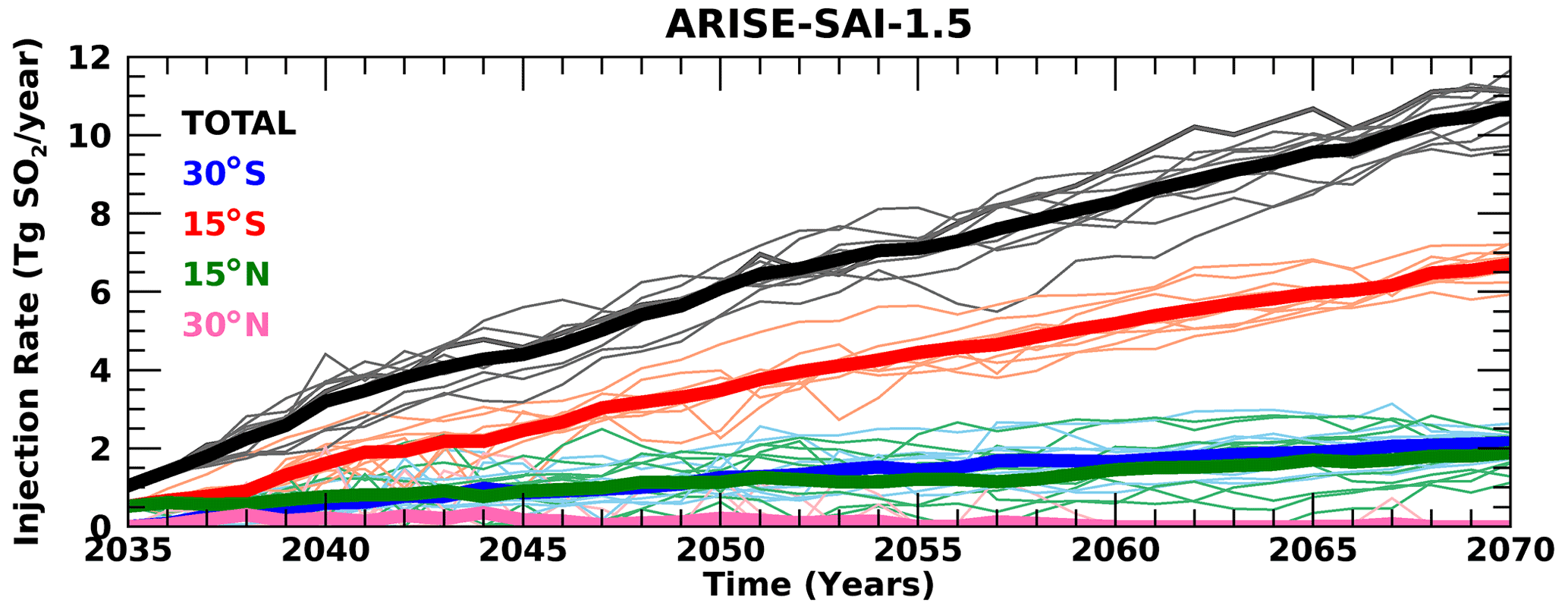
Figure 1SO2 injection rate as a function of time in ARISE-SAI-1.5 simulations at 30∘ S (blue), 15∘ S (red), 15∘ N (green), 30∘ N (pink), and total (black). Thin lighter-colored lines represent individual ensemble members, whereas thick lines show the 10-member ensemble mean.
The amount of SO2 injection in the ARISE-SAI-1.5 simulations chosen by the controller algorithm is shown in Fig. 1. The majority of SO2 is injected at 15∘ S, with an approximate linear increase from 0.5 Tg SO2 per year in 2035 to 6 Tg SO2 per year in 2069. SO2 injections at 30∘ S and 15∘ N are about of that injected at 15∘ S. Throughout all the ARISE-SAI-1.5 simulations, the amount of SO2 injection at 30∘ N is very small at less than 0.5 Tg SO2 per year, diminishing to nearly zero by the end of the simulations. The distribution of SO2 across the four injection latitudes in ARISE-SAI-1.5 is very different from that in GLENS (Tilmes et al., 2018) despite having the same goals for the controller. In GLENS, the majority of SO2 was injected at 30∘ S and 30∘ N, with a significant amount at 15∘ N and almost none at 15∘ S; that is, GLENS required more injection in the Northern Hemisphere than the Southern Hemisphere in order to maintain the interhemispheric temperature gradient T1, whereas ARISE-SAI-1.5 requires more injection in the Southern Hemisphere to maintain T1. GLENS also required more SO2 injection at 30∘ N, 30∘ S to maintain T2 than is required in ARISE-SAI-1.5. It is unclear at this time how much of this difference is a result of the different model version and how much is a result of changes in the forcing between RCP8.5 and SSP2–4.5.
One of the intents of ARISE-SAI simulations is to provide the broader community with a dataset for examining various impacts of SCI on the multiple components of the Earth system. Below we present basic diagnostics that verify that the SO2 injections and controller are working as intended, and we describe how well the temperature targets are being met in CESM2(WACCM6). Detailed analysis of the simulations is left for future work.

Figure 2Zonal mean stratospheric SO4 concentration increase (in µg S kg−1 of air) in (a) 2035–2054 and (c) 2050–2069 relative to the 2020–2039 mean. Black contour lines show the background concentration in 2020–2039. Blue line shows the annual mean tropopause height in the control period; the red line shows the annual mean tropopause height in the ARISE simulation in 2035–2054 and 2050–2069. Gray shading indicates the grid boxes where SO2 is injected. The zonal mean total increase in the column burden of sulfate (in mg SO4 m−2) for (b) 2035–2054 and (d) 2050–2069. The contribution to the column increase is shown in dark red for the fraction located in the stratosphere and in orange for the fraction located in the troposphere.
4.1 Stratospheric aerosols
Injection of sulfur dioxide into the stratosphere results in the formation of sulfate aerosols, which are transported by the stratospheric Brewer–Dobson circulation (Andrews et al., 1987; Tilmes et al., 2017). The dominance of SO2 injections at 15∘ S in ARISE-SAI-1.5 results in a stratospheric sulfate (SO4) increase that primarily occurs in the Southern Hemisphere, with the majority of SO4 concentrated near the primary injection location (Fig. 2a and b). Averaged over the 2035–2054 period, there is a peak SO4 increase of 25 mg S kg−1 air (Fig. 2a) relative to the 2020–2039 mean, and averaged over 2050–2069 an SO4 increase of 48 mg S kg−1 air is found near 15∘ S at 40 hPa (Fig. 2b). The zonally averaged latitudinal distribution of the increase in the column of SO4 is shown in Fig. 2c and d; both show the strong hemispheric asymmetry as well as a double peak at around 15∘ S and one near 50∘ S. The peak near 15∘ S is due to the predominant location of the injection and matches the peak in concentration; the latter is due to the largest vertical stratospheric layer over which SO4 is spread out (between 10 and 22 km) compared to the layer in the tropical stratosphere (between 18 and 26 km). Integrated over 20-year periods of ARISE-SAI-1.5 simulations, there is little difference in the latitudinal distribution of column SO4 between the various ensemble members, but amplitude differences of up to 15 % exist (not shown), reflecting variability in the amount of SO2 injection at each location and small differences in the stratospheric circulation.
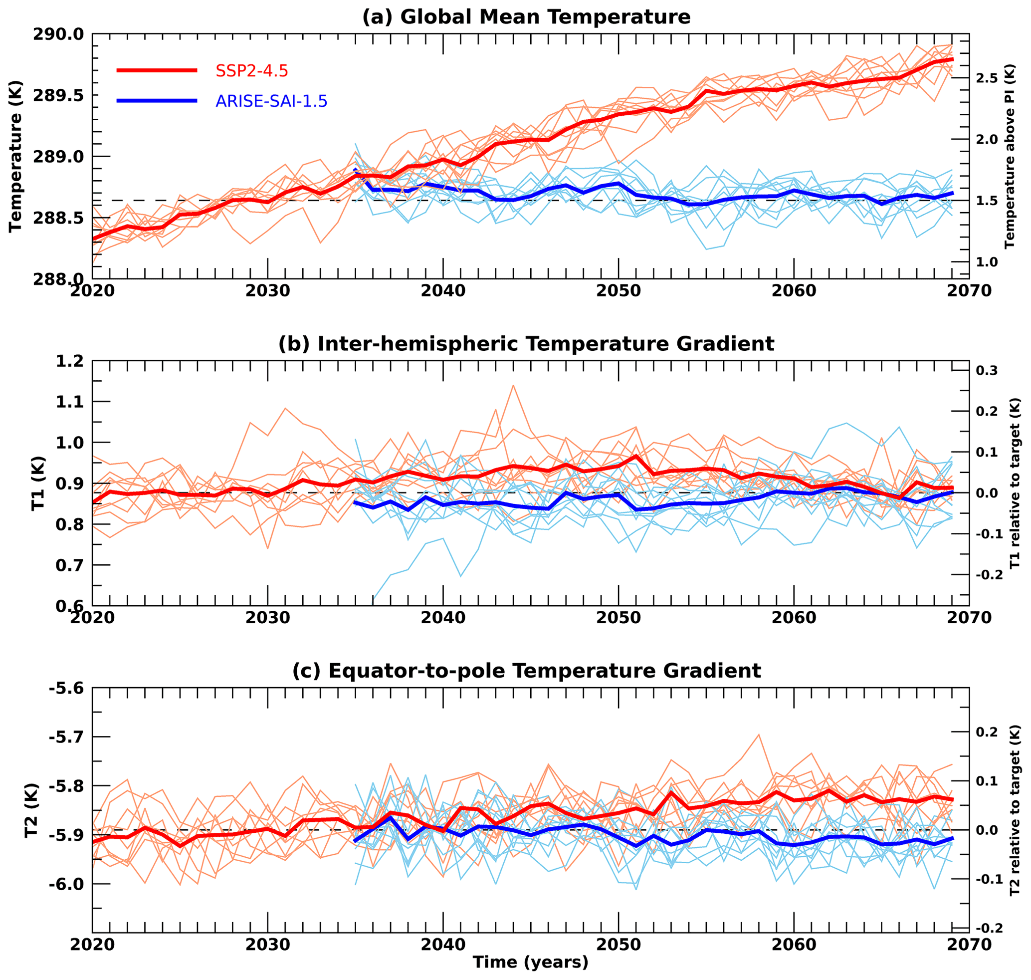
Figure 3Global mean (a) surface temperature, (b) interhemispheric temperature gradient, T1, and (c) Equator-to-pole temperature gradient, T2, for SSP2–4.5 (red) and ARISE-SAI-1.5 (blue) simulations. Thin lines represent individual ensemble members, whereas the thick lines show the ensemble mean.
4.2 Meeting temperature targets
Global mean surface temperature, the interhemispheric temperature gradient, and Equator-to-pole temperature gradients for the SSP2–4.5 and ARISE-SAI-1.5 simulations are shown in Fig. 3. There is a notable difference in behavior of T1 and T2 in the SSP2–4.5 simulations compared to the RCP8.5 simulations with CESM1(WACCM) (not shown). In the CESM1(WACCM) simulations with RCP8.5, T1 and T2 increased steadily with time of simulation, reaching a change in T1 of nearly 0.45 K and a T2 change of 0.3 K by 2070 relative to the ∼2020–2039 mean (Tilmes et al., 2018). In contrast, T1 and T2 in the SSP2–4.5 simulation increase much more slowly by less than 0.05 K for T1 and less than 0.1 K for T2 between the reference period (2020–2039) and 2070. The more moderate (SSP2–4.5) emission scenario used in the CESM2(WACCM6) control simulations partially explains the slower increase in T1 and T2 with time, but not all. Simulations with CESM2(WACCM6) and SSP5–8.5 scenarios also show a much slower increase in T1 and T2 compared to CESM1(WACCM) with RCP8.5. Differing modeling physics, in particular cloud feedbacks, between CESM1 and CESM2 are key differences that could lead to the differences in projected spatial patterns of surface warming between the two model configurations, as well as changes in the Atlantic Meridional Overturning Circulation as discussed in Tilmes et al. (2020). Additional simulations with CESM2 and RCP emissions have been performed to understand the relative role of differences in forcing and differences in model physics in projected spatial patterns of global mean temperature and other variables between CESM1 and CESM2. A detailed discussion of the reasons behind the model dependence on injection strategy in GLENS, CESM1(WACCM), and ARISE-SAI-1.5, CESM2(WACCM6) simulations can be found in Fasullo and Richter (2022). They show that the main contributors to the differences are rapid adjustment of clouds and rainfall to elevated levels of carbon dioxide, dynamical responses in the Atlantic Meridional Overturning Circulation (AMOC), and differences in future climate forcing scenarios.
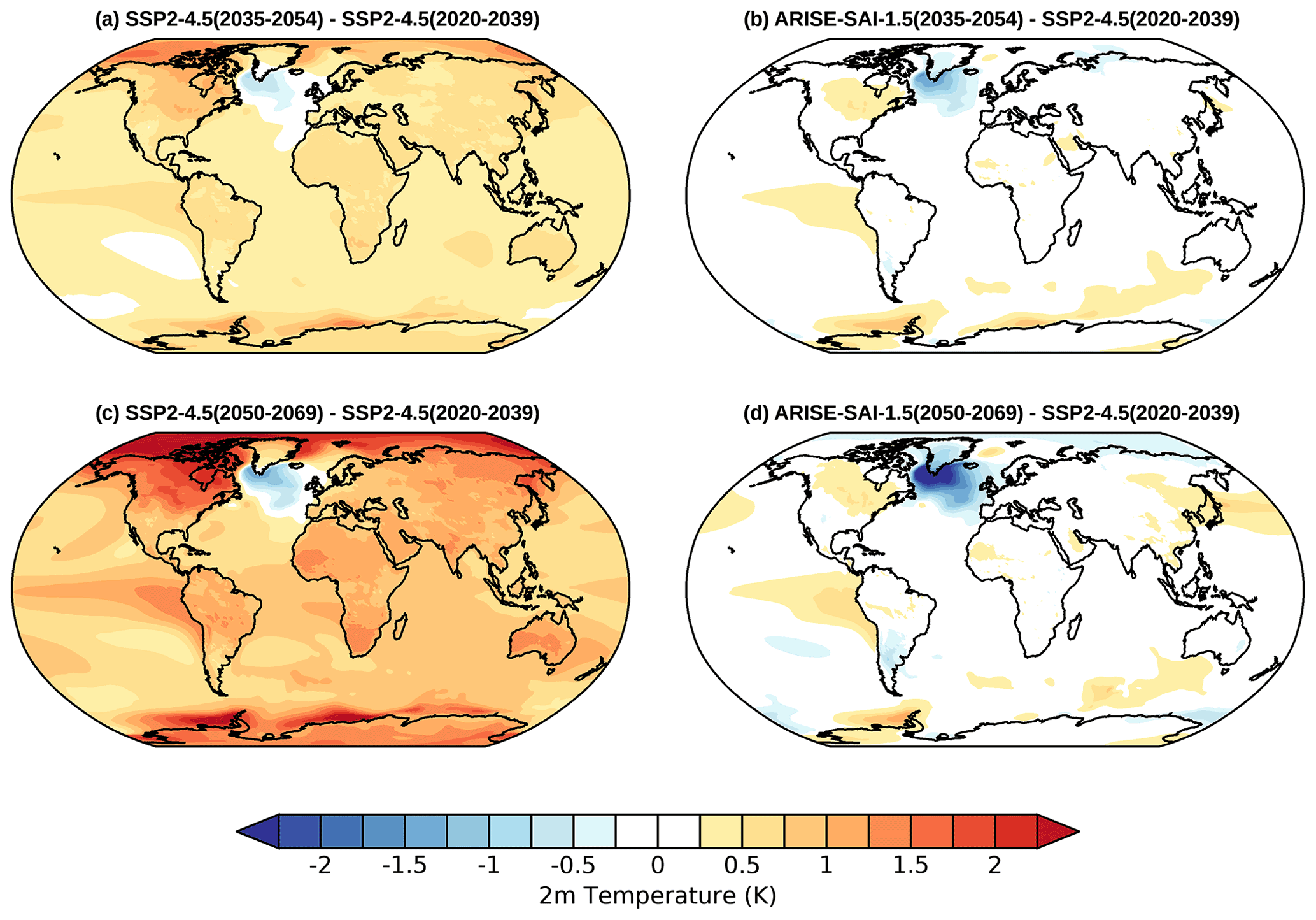
Figure 4Ensemble and annual mean surface (2 m) temperature differences between (a) SSP2–4.5 (2035–2054) and SSP2–4.5 (2020–2039), (b) ARISE-SAI-1.5 (2035–2054) and SSP2–4.5 (2020–2039), (c) SSP2–4.5 (2050–2069) and SSP2–4.5 (2020–2039), and (d) ARISE-SAI-1.5 (2050–2069) and SSP2–4.5 (2020–2039). Gray shading indicates regions where the differences are not statistically significant at the 95 % level using a two-sided Student's t test.
The differences between the projected surface temperature patterns in CESM2 compared to CESM1 have implications for climate intervention. Since the changes in T1 and T2 targets differ between the CESM1(WACCM) and CESM2(WACCM6) future simulations, the controller selects different SO2 injection locations to best counteract these changes. Injections needed to offset increasing T1 and T2 in CESM1(WACCM) required primarily injections at 30∘ S and 30∘ N, whereas for a small change in T1 and T2 relative to the 2020–2039 period in CESM2(WACCM6), SSP2–4.5 requires injections primarily at 30∘ S. The SO2 injections applied in ARISE-SAI-1.5 do a very good job at keeping the global mean temperature, T1, and T2 at the target levels. This is demonstrated by the blue lines in Fig. 2. There is a fair amount of variability among the individual ensemble members (thin light blue lines) in their ability to meet the global mean T1 and T2 targets; however, the ensemble mean (thick blue line) shows very good agreement between these variables and their target values.
4.3 Surface temperature and precipitation
Figure 4 shows the ensemble and annual mean surface temperature changes for two time periods, 2035–2054 and 2050–2069, during the SSP2–4.5 and ARISE-SAI-1.5 simulations relative to the 2020–2039 period. Figure 4a and c show the steady increase in surface temperature with time over the majority of the globe, with the largest warming occurring in the Northern Hemisphere high latitudes. The North Atlantic is the only region of the globe that is cooling in the 21st century. This “warming hole” in the North Atlantic is a feature of several recent-generation Earth system models and is attributed to the AMOC (Drijfhout et al., 2012; Chemke et al., 2020; Keil et al., 2020). Specifically, in a warming climate with a reduction in deepwater formation, the AMOC weakens. This results in less heat transport into the northern North Atlantic, producing cooler temperatures that oppose the anticipated effects of global warming. Figure 4b and d demonstrate the success of the SAI strategy in keeping the global temperatures near the 2020–2039 average, or at ∼1.5 K above pre-industrial values. In ARISE-SAI-1.5, near-surface annual mean temperature throughout the entire simulation is within 0.5 K of that goal over the majority of the globe. The largest exception to that is the North Atlantic warming hole, where surface temperatures remain cooler relative to the northern North Atlantic than in the present day; while AMOC strength is partially recovered under SAI relative to SSP2–4.5, it is not fully restored back to present-day conditions. In addition, in the ensemble mean, ARISE-SAI-1.5 simulations show residual warming over North America, as well as over eastern South Pacific Ocean (off the coast of South America) and in parts of Antarctica compared to the 2020–2039 period. Residual changes relative to the target period from the application of SAI are expected, as SAI cannot perfectly reverse the effects of increasing greenhouse gases.
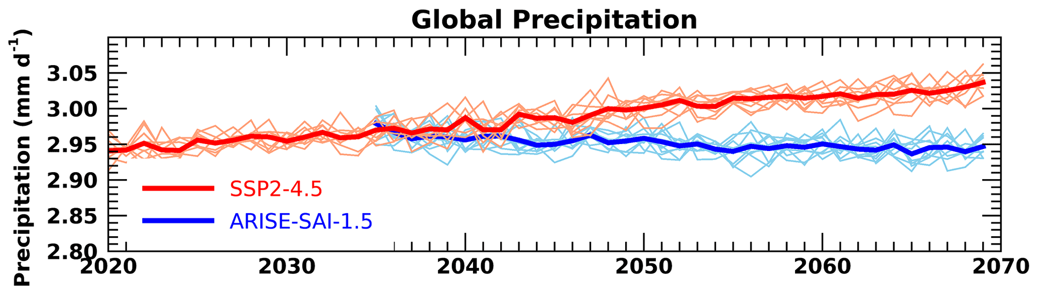
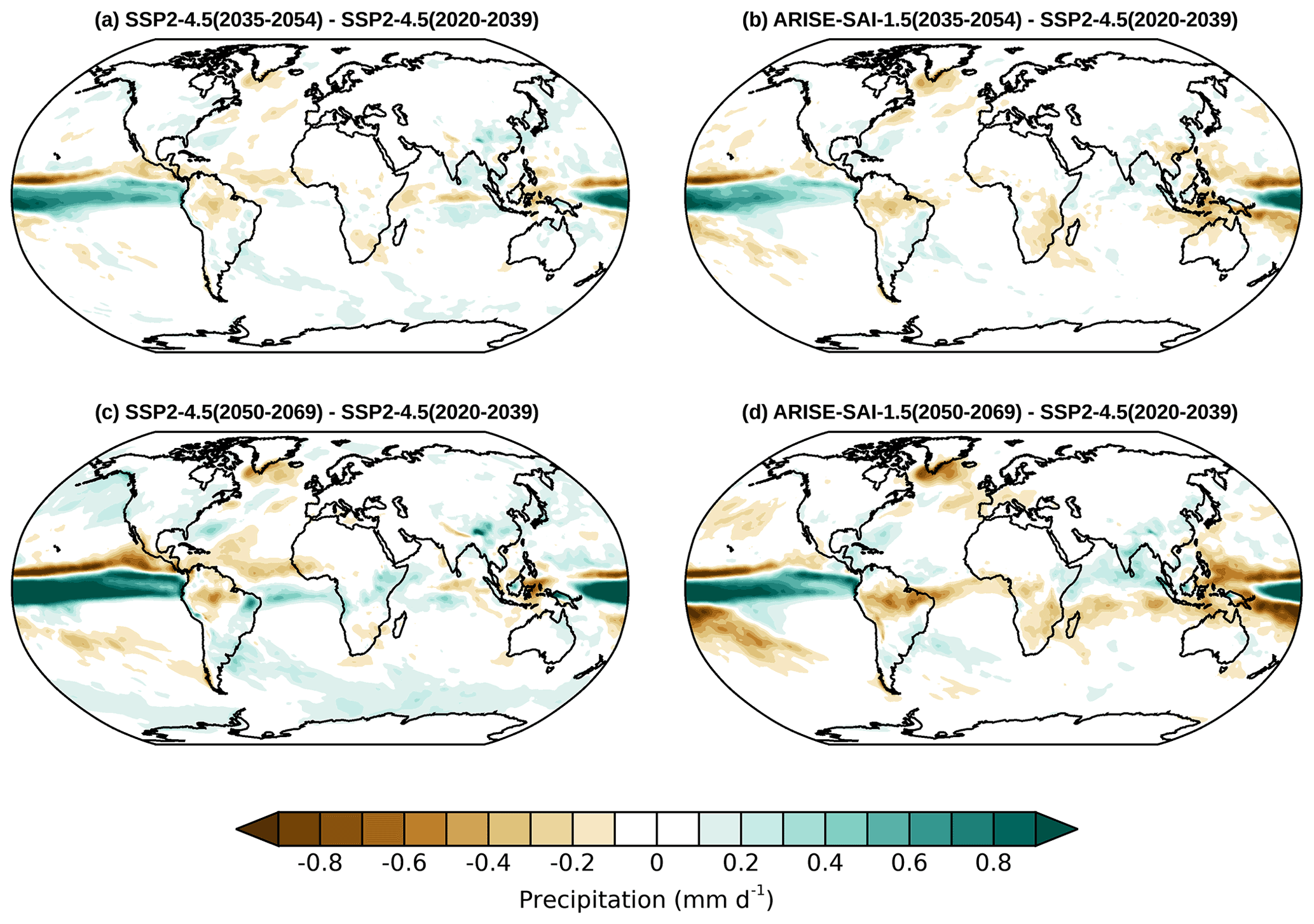
Figure 6Same as Fig. 4 but for annual mean precipitation.
The precipitation changes in SSP2–4.5 and ARISE-SAI-1.5 simulations for the same time periods examined for surface temperature changes are shown in Figs. 5 and 6. Consistent with prior similar studies, SSP2–4.5 simulations primarily show an increase in precipitation in a warming climate, with the largest increases along the equatorial Pacific Ocean and a strong drying region northward of that (Figs. 5, 6a and c). In ARISE-SAI-1.5, consistent with previous studies (Kravitz et al., 2017; Lee et al., 2020), restoring global mean temperature is associated with an overall decrease in annual mean precipitation (Fig. 5); however, regionally both increases and decreases occur. In ARISE-SAI-1.5, the increased precipitation across the equatorial Pacific seen in SSP2–4.5 decreases in magnitude but is still a persistent feature. ARISE-SAI-1.5 also shows drying north and south of that region as well as intensified drying over northern South America, South Africa, the Indian Ocean south of the Equator, and northernmost Australia. The Indian Ocean north of the Equator and India are projected to be wetter in ARISE-SAI-1.5 compared to the 2020–2039 period of SSP2–4.5.
We have described a detailed new modeling protocol and the first set of simulations of Assessing Responses and Impacts of Solar climate intervention on the Earth system with stratospheric aerosol injection (ARISE-SAI) for studies of impacts of climate intervention using stratospheric aerosols. We have carried out the ARISE-SAI-1.5 simulations utilizing CESM2(WACCM6) and provided extensive output for community analysis. The protocol for simulations described here can be easily implemented in other Earth system models with similar capabilities; furthermore, the protocol can easily be adapted to explore different climate intervention scenarios considering other climate targets, such as different global mean cooling targets, and in the future extended to other types of climate intervention, such as marine cloud brightening. The SAI strategy defined by the protocol builds on the approach used in GLENS that was carried out with CESM1(WACCM), but uses a more moderate background emissions scenario, a start date of 2035 rather than 2020, and a target temperature of 1.5 ∘C over pre-industrial following the AR6 definition; the set of simulations presented here also uses a newer version of CESM, which is the same as used for CMIP6 (Gettelman et al., 2019). In these new simulations, the SO2 injections required to keep the global mean temperature, interhemispheric temperature gradient, and pole-to-pole temperature gradient at the target level in ARISE-SAI-1.5 are needed primarily at 15∘ S, in contrast to GLENS, which utilized SO2 injections primarily at 30∘ N and 30∘ S. The reasons for these differences are currently being investigated in detail, and it highlights the need to reproduce such experiments with other climate models to understand their sources. Surface climate in ARISE-SAI-1.5 is very similar to that during the reference period (2020–2039); however, residual changes still remain, in particular in the North Atlantic, where surface temperature is cooler than in the reference period. The robustness of these projected regional residuals in other climate models, or under different climate targets, would also be of extreme interest. Consistent with prior studies, global mean precipitation in ARISE-SAI-1.5 is smaller than during the reference period.
The output for the ARISE-SAI-1.5 simulations is extensive and includes variables from multiple Earth system components, enabling the community analysis of changes in many variables that are crucial to making decisions about the implementation of SCI including weather and climate extremes, crops, and ozone changes. To enable broad access to the data, output from the ARISE-SAI-1.5 simulations is available on the Amazon Web Services Open Data portal.
Table A1Minimum recommended monthly mean output for ARISE-SAI simulations and corresponding reference simulations.
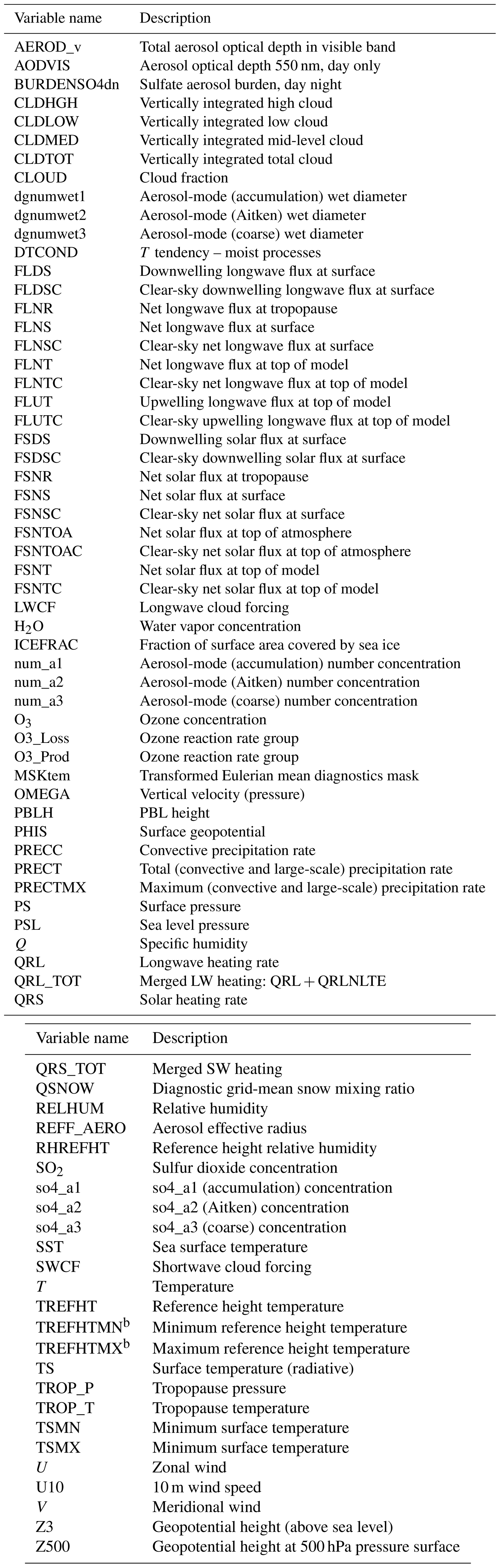
Table A2Available daily averaged output from the atmospheric model in ARISE-SAI-1.5 simulations and SSP2–4.5 CESM2(WACCM6) simulations. a Variables not available from the first five members of CESM2(WACCM6) SSP2–4.5 simulations. b Variables that are available (but erroneous) in the first five members of CESM2(WACCM6) SSP2–4.5 simulations. Variables in bold are used to calculate indices of extremes such as those presented in Tye et al. (2022).
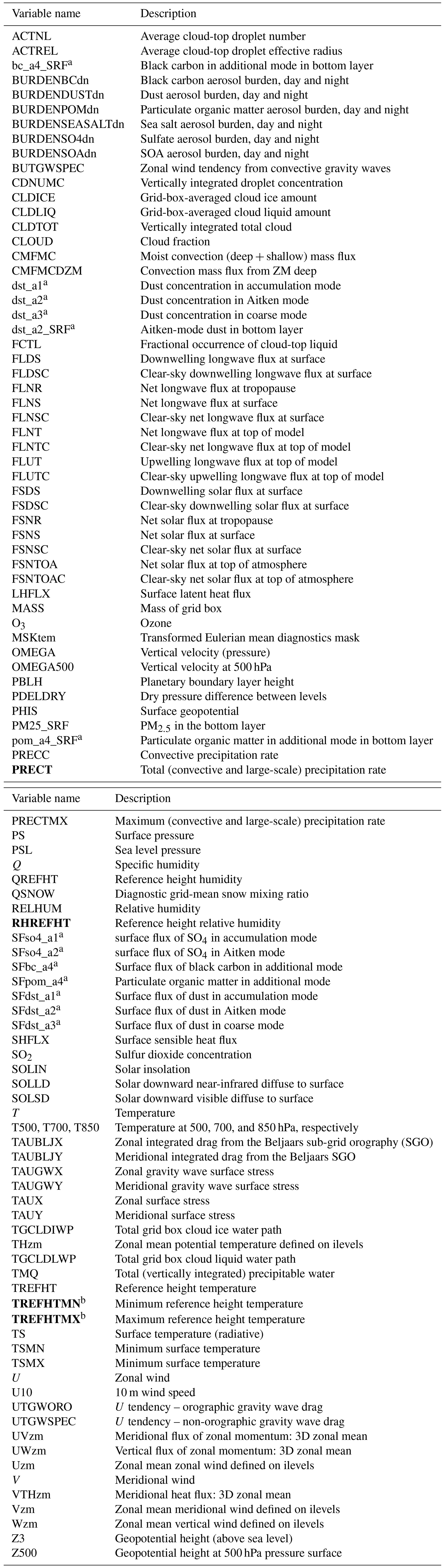
Table A33-hourly averaged output from the atmospheric model in ARISE-SAI-1.5 simulations and five additional SSP2–4.5 CESM2(WACCM6) simulations. None of the above output is contained in the first five ensemble members of CESM2(WACCM6) SSP2–4.5 simulations.
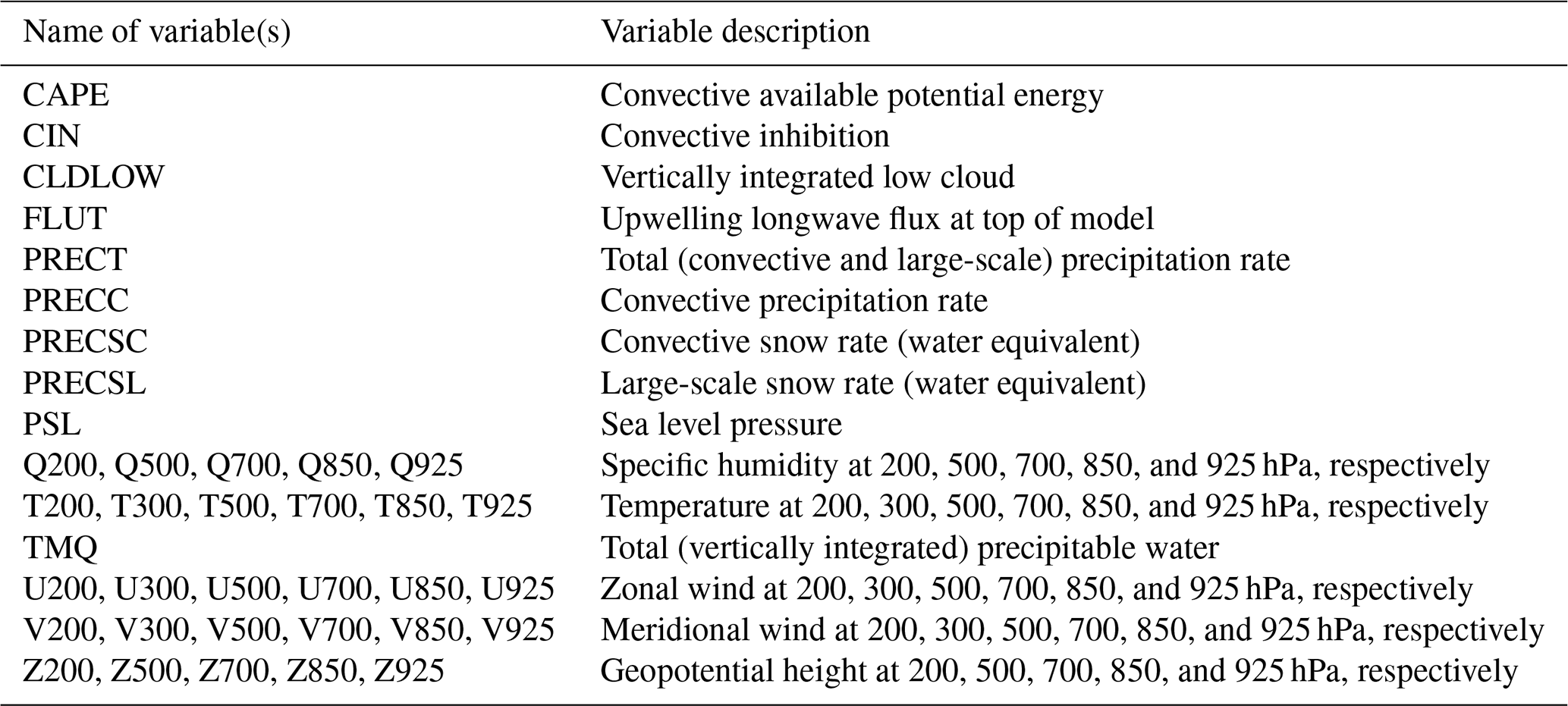
Table A43-hourly instantaneous output from the atmospheric model in ARISE-SAI-1.5 simulations and five additional SSP2–4.5 CESM2(WACCM6) simulations. For the variables marked with an asterisk (∗), only the bottommost 22 levels were retained; hence, levels for those variables range from 1000 to 103 hPa. None of the above output is contained in the first five ensemble members of CESM2(WACCM6) SSP2–4.5 simulations.
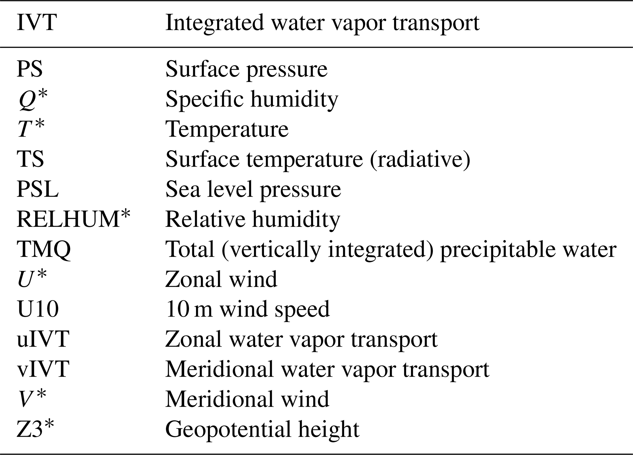
Table A51-hourly instantaneous output from the atmospheric model in ARISE-SAI-1.5 simulations and five additional SSP2–4.5 CESM2(WACCM6) simulations. None of the above output is contained in the first five ensemble members of CESM2(WACCM6) SSP2–4.5 simulations.

Table A6Available daily averaged output from the land model at land unit level in ARISE-SAI-1.5 simulations and five additional SSP2–4.5 CESM2(WACCM6) simulations. None of the above output is contained in the first five ensemble members of CESM2(WACCM6) SSP2–4.5 simulations.
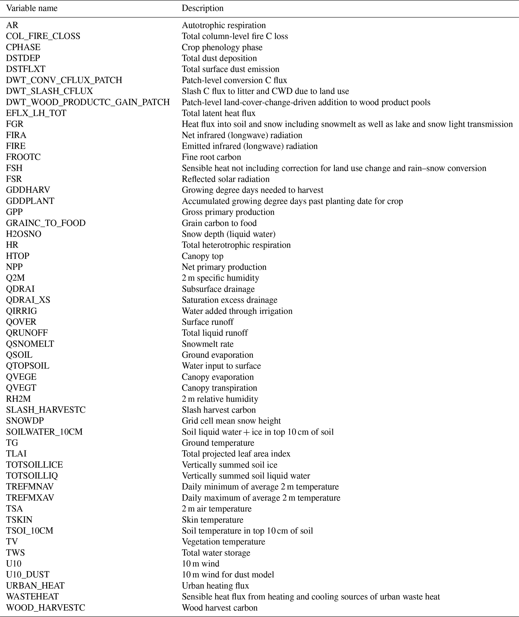
Table A7Available daily averaged output from the land model at grid cell level in ARISE-SAI-1.5 simulations and five additional SSP2–4.5 CESM2(WACCM6) simulations. None of the above output is contained in the first five ensemble members of CESM2(WACCM6) SSP2–4.5 simulations.
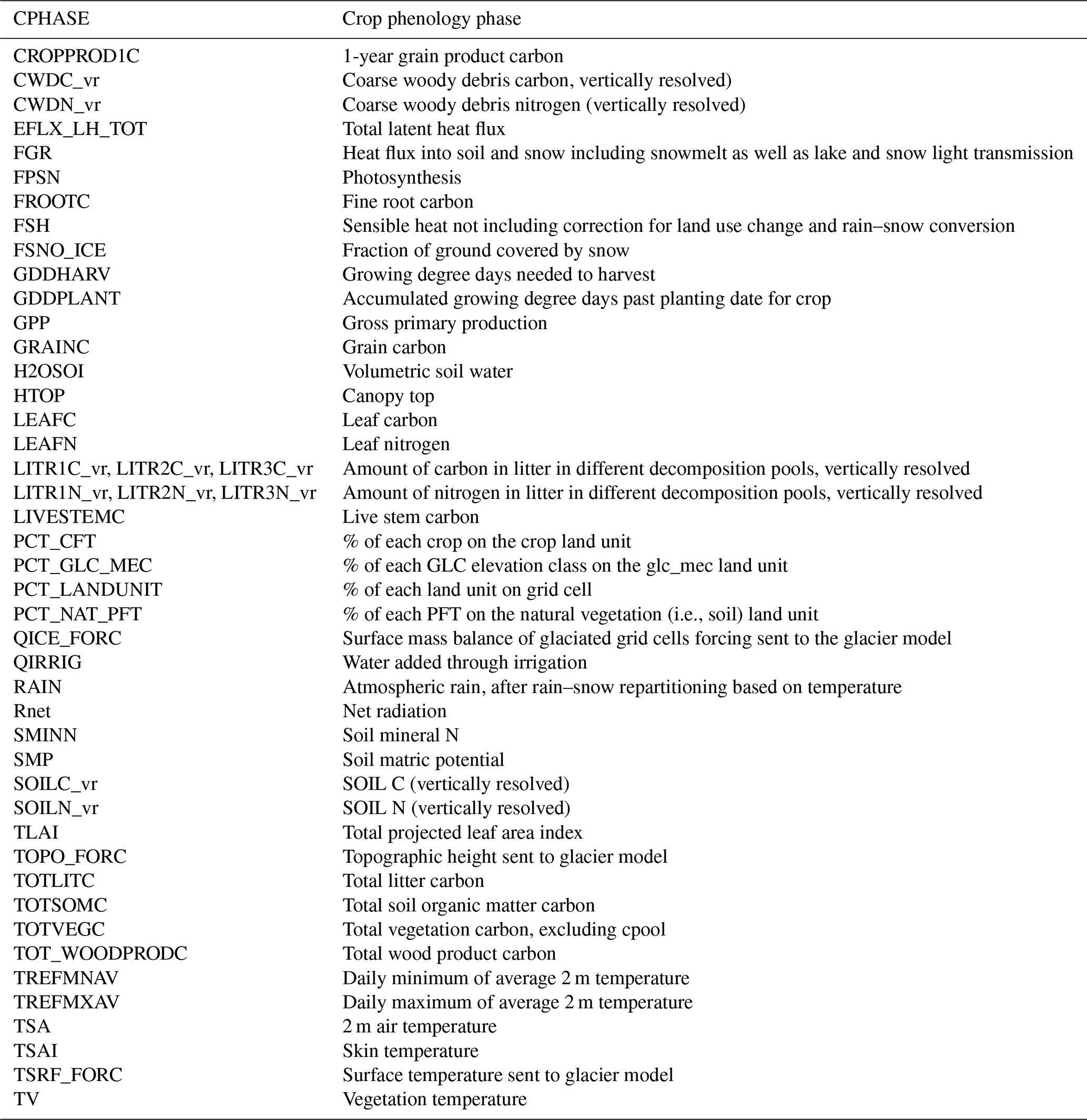
Table A86-hourly averaged output from the land model in ARISE-SAI-1.5 simulations and five additional SSP2–4.5 CESM2(WACCM6) simulations. None of the above output is contained in the first five ensemble members of CESM2(WACCM6) SSP2–4.5 simulations.
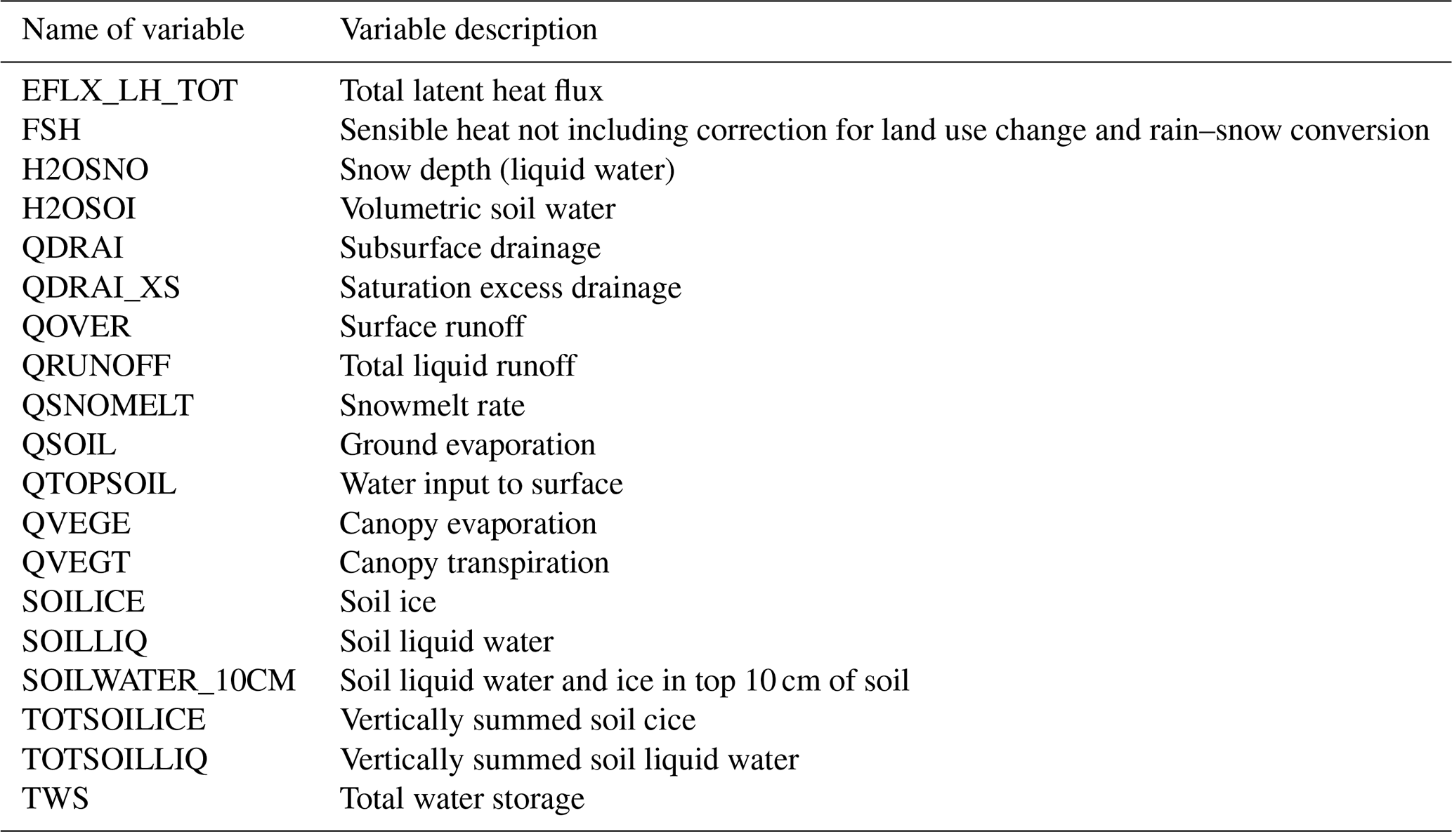
Table A9Daily averaged output from the ocean model in ARISE-SAI-1.5 simulations and all SSP2–4.5 CESM2(WACCM6) simulations.

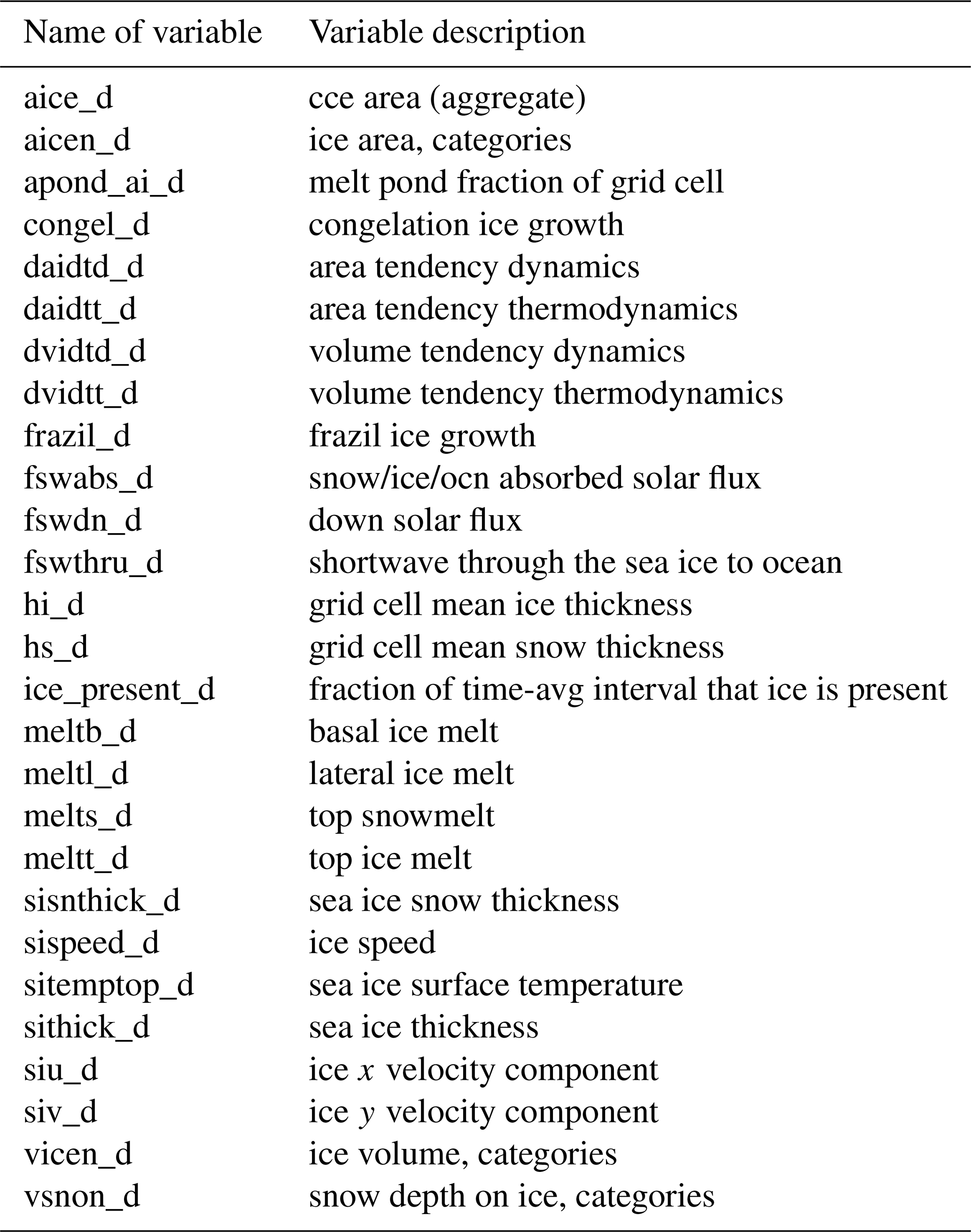
Table A10Daily averaged output from the sea ice model in ARISE-SAI-1.5 simulations and all SSP2–4.5 CESM2(WACCM6) simulations.
CESM tag cesm2.1.4-rc.08 was used to carry out the simulations and is also available at https://doi.org/10.5281/zenodo.7271743 (CESM Team, 2022). Python scripts to generate the case directories with appropriate model tags and output can be found at https://doi.org/10.5281/zenodo.6474201 (Rosenbloom, 2022). The code for the SO2 injection controller can be downloaded from https://doi.org/10.5281/zenodo.6471092 (Kravitz and Visioni, 2022).
All the data presented in this paper are available at https://doi.org/10.5281/zenodo.6473954 (Richter and Visioni, 2022a) from the CESM2(WACCM6) SSP2–4.5 simulations and at https://doi.org/10.5281/zenodo.6473775 (Richter and Visioni, 2022b) from the ARISE-SAI-1.5 simulations. Complete output from all 10 members of CESM2(WACCM6) SSP2–4.5 simulations and ARISE-SAI-1.5 simulations is freely available the NCAR Climate Data Gateway at https://doi.org/10.26024/0cs0-ev98 (Mills et al., 2022) and https://doi.org/10.5065/9kcn-9y79 (Richter, 2021), respectively. The ARISE-SAI-1.5 and SSP-4.5 datasets are additionally available for free download through the Amazon/AWS Open Data program. These can be accessed at https://registry.opendata.aws/ncar-cesm2-arise/ (Richter et al., 2022). We anticipate community analysis of various aspects of the Earth system of the ARISE-SAI-1.5 simulations. There is no obligation to inform the project authors about the analysis you are performing, but it would be helpful to reach out to DV in order to coordinate analysis and avoid duplicate efforts.
JHR designed and carried out simulations, compiled output requests, created most of the figures, and drafted the paper. DV set up the injection controller, carried out simulations, created a figure, and wrote parts of the paper. DGM co-designed the simulations and helped with interpretation of results. DAB created the time series of and archived all the data. NR created namelists with desired output and scripts to easily set up the simulations. BD set up the AWS data hosting site and transferred all the output there. WRL analyzed the control simulations and provided targets for the controller. MT and JFL gave input to simulation design and data output requests. All authors reviewed the paper.
The contact author has declared that none of the authors has any competing interests.
Publisher's note: Copernicus Publications remains neutral with regard to jurisdictional claims in published maps and institutional affiliations.
This material is based upon work supported by the National Center for Atmospheric Research, which is a major facility sponsored by the National Science Foundation under cooperative agreement no. 1852977 and by SilverLining through its Safe Climate Research Initiative. The Community Earth System Model (CESM) project is supported primarily by the National Science Foundation. Computing and data storage resources, including the Cheyenne supercomputer (https://doi.org/10.5065/D6RX99HX; NCAR CISL Advanced Research Computing, 2021), were provided by the Computational and Information Systems Laboratory (CISL) at NCAR. Cloud storage support is provided through the Amazon Sustainability Data Initiative. We thank two anonymous reviewers for their comments that improved the paper.
This research has been supported by the National Science Foundation (grant no. 1852977) and by SilverLining through its Safe Climate Research Initiative.
This paper was edited by Juan Antonio Añel and reviewed by two anonymous referees.
Andrews, D. G., Holton, J. R., and Leovy, C. B.: Middle atmosphere dynamics, Academic Press, San Diego, CA, xi + 489, 1987.
Bingaman, D. C., Rice, C. V., Smith, W., and Vogel, P.: A Stratospheric Aerosol Injection Lofter Aircraft Concept: Brimstone Angel, AIAA 2020-0618, AIAA Scitech 2020 Forum, January 2020.
Burgess, M. G., Ritchie, J., Shapland, J., and Pielke Jr., R.: IPCC baseline scenarios have over-projected CO2 emissions and economic growth, Environ. Res. Lett., 16, 014016, https://doi.org/10.1088/1748-9326/abcdd2, 2020.
Carlson, C. J. and Trisos, C. H.: Climate engineering needs a clean bill of health, Nat. Clim. Change, 8, 843–845, https://doi.org/10.1038/s41558-018-0294-7, 2018.
CESM Team: CESM2.1.4-rc.07, Zenodo [code], https://doi.org/10.5281/zenodo.7271743, 2022.
Chemke, R., Zanna, L., and Polvani, L. M.: Identifying a human signal in the North Atlantic warming hole, Nat. Commun., 11, 1–7, 2020.
Coburn, J. and Pryor, S. C.: Differential Credibility of Climate Modes in CMIP6, J. Climate, 34, 8145–8164, 2021.
Danabasoglu, G., Bates, S. C., Briegleb, B. P., Jayne, S. R., Jochum, M., Large, W. G., Peacock, S., and Yeager, S. G.: The CCSM4 ocean component, J. Climate, 25, 1361–1389. https://doi.org/10.1175/JCLI-D-11-00091.1, 2012.
Danabasoglu, G., Lamarque, J.-F., Bacmeister, J., Bailey, D. A., DuVivier, A. K., Edwards, J., Emmons, L. K., Fasullo, J., Garcia, R., Gettelman, A., Hannay, C., Holland, M. M., Large, W. G., Lauritzen, P. H., Lawrence, D. M., Lenaerts, J. T. M., Lindsay, K., Lipscomb, W. H., Mills, M. J., Neale, R., Oleson, K. W., Otto-Bliesner, B., Phillips, A. S., Sacks, W., Tilmes, S., van Kampenhout, L., Vertenstein, M., Bertini, A., Dennis, J., Deser, C., Fischer, C., Fox-Kemper, B., Kay, J. E., Kinnison, D., Kushner, P. J., Larson, V. E., Long, M. C., Mickelson, S., Moore, J. K., Nienhouse, E., Polvani, L., Rasch, P. J., and Strand, W. G.: The Community Earth System Model Version 2 (CESM2), J. Adv. Model. Earth Sy., 12, e2019MS001916, https://doi.org/10.1029/2019MS001916, 2020.
Deser, C., Phillips, A., Bourdette, V., and Teng, H.: Uncertainty in climate change projections: the role of internal variability, Clim. Dynam., 38, 527–546, https://doi.org/10.1007/s00382-010-0977-x, 2012.
Drijfhout, S., van Oldenborgh, G. J., and Cimatoribus, A.: Is a Decline of AMOC Causing the Warming Hole above the North Atlantic in Observed and Modeled Warming Patterns?, J. Climate, 25, 8373–8379, https://doi.org/10.1175/JCLI-D-12-00490.1, 2012.
DuVivier, A. K., Holland, M. M., Kay, J. E., Tilmes, S., Gettelman, A., and Bailey, D. A.: Arctic and Antarctic sea ice mean state in the Community Earth System Model Version 2 and the influence of atmospheric chemistry, J. Geophys. Res.-Oceans, 125, e2019JC015934, https://doi.org/10.1029/2019JC015934, 2020.
Eyring, V., Bony, S., Meehl, G. A., Senior, C. A., Stevens, B., Stouffer, R. J., and Taylor, K. E.: Overview of the Coupled Model Intercomparison Project Phase 6 (CMIP6) experimental design and organization, Geosci. Model Dev., 9, 1937–1958, https://doi.org/10.5194/gmd-9-1937-2016, 2016.
Fasullo, J. T. and Richter, J. H.: Scenario and Model Dependence of Strategic Solar Climate Intervention in CESM, EGUsphere [preprint], https://doi.org/10.5194/egusphere-2022-779, 2022.
Gettelman, A., Mills, M. J., Kinnison, D. E., Garcia, R. R., Smith, A. K., Marsh, D. R., Times, S., Vitt F., Bardeen, C. G., McInerny, J., Liu, H.-L., Solomon, S. C., Polvani, L. M., Emmons, L. K., Lamarque, J.-F., Richter, J. H., Glanville, A. S., Bacmeister, J. T., Philips, A. S., Neale, R. B., Simpson, I. R., DuVivier, A. K., Hodzic, A., and Randel, W. J.: The whole atmosphere community climate model version 6 (WACCM6), J. Geophys. Res.-Atmos., 124, 12380–12403, https://doi.org/10.1029/2019JD030943, 2019.
Hausfather, Z. and Peters, G. P.: Emissions – “business as usual” story is misleading, Nature, 577, 618–620, https://doi.org/10.1038/d41586-020-00177-3, 2020.
Hunke, E. C., Lipscomb, W. H., Turner, A. K., Jeffery, N., and Elliott, S.: CICE: The Los Alamos Sea Ice Model. Documentation and Software User's Manual. Version 5.1, T-3 Fluid Dynamics Group, Los Alamos National Laboratory, Tech. Rep. LA-CC-06-012, 2015.
IPCC: Global Warming of 1.5 ∘C. An IPCC Special Report on the impacts of global warming of 1.5 ∘C above pre-industrial levels and related global greenhouse gas emission pathways, in the context of strengthening the global response to the threat of climate change, sustainable development, and efforts to eradicate poverty, edited by: Masson-Delmotte, V., Zhai, P., Pörtner, H.-O., Roberts, D., Skea, J., Shukla, P. R., Pirani, A., Moufouma-Okia, W., Péan, C., Pidcock, R., Connors, S., Matthews, J. B. R., Chen, Y., Zhou, X., Gomis, M. I., Lonnoy, E., Maycock, T., Tignor, M., and Waterfield, T., Cambridge University Press, Cambridge, UK and New York, NY, USA, 616 pp., https://doi.org/10.1017/9781009157940, 2018.
IPCC: Climate Change 2021: The Physical Science Basis. Contribution of Working Group I to the Sixth Assessment Report of the Intergovernmental Panel on Climate Change, edited by: Masson-Delmotte, V., Zhai, P., Pirani, A., Connors, S. L., Péan, C., Berger, S., Caud, N., Chen, Y., Goldfarb, L., Gomis, M. I., Huang, M., Leitzell, K., Lonnoy, E., Matthews, J. B. R., Maycock, T. K., Waterfield, T., Yelekçi, O., Yu, R., and Zhou, B., Cambridge University Press, 2391 pp., https://doi.org/10.1017/9781009157896, 2021.
Kay, J. E., Deser, C., Phillips, A., Mai, A., Hannay, C., Strand, G., Arblaster, J. M., Bates, S. C., Danabasoglu, G., Edwards, J., Holland, M., Kushner, P., Lamarque, J.-F., Lawrence, D., Lindsay, K., Middleton, A., Munoz, E., Neale, R., Oleson, K., Polvani, L., and Vertenstein, M.: The Community Earth System Model (CESM) Large Ensemble Project: A Community Resource for Studying Climate Change in the Presence of Internal Climate Variability, B. Am. Meteorol. Soc., 96, 1333–1349, 2015.
Keil, P., Mauritsen, T., Jungclaus, J. Hedemann, C., Olonscheck, D., and Ghosh, R.: Multiple drivers of the North Atlantic warming hole, Nat. Clim. Chang., 10, 667–671, https://doi.org/10.1038/s41558-020-0819-8, 2020.
Kravitz, B. and MacMartin, D. G.: Uncertainty and the basis for confidence in solar geoengineering research, Nat. Rev. Earth Environ., 1, 64–75, https://doi.org/10.1038/s43017-019-0004-7, 2020.
Kravitz, B. and Visioni, D.: Explicit Feedback for Climate Modeling, Zenodo [code], https://doi.org/10.5281/zenodo.6471092, 2022.
Kravitz, B., Caldeira, K., Boucher, O., Robock, A., Rasch, P. J., Alterskjær, K., Karam, D. B., Cole, J. N. S., Curry, C. L., Haywood, J. M., Irvine, P. J., Ji, D., Jones, A., Kristjánsson, J. E., Lunt, D. J., Moore, J. C., Niemeier, U., Schmidt, H., Schulz, M., Singh, B., Tilmes, S., Watanabe, S., Yang, S., and Yoon, J.-H.: Climate model response from the Geoengineering Model Intercomparison Project (GeoMIP), J. Geophys. Res.-Atmos., 118, 8320–8332, https://doi.org/10.1002/jgrd.50646, 2013.
Kravitz, B., MacMartin, D. G., Mills, M. J., Richter, J. H., Tilmes, S., Lamarque, J.-F., Tribbia, J. J., and Vitt, F.: First simulations of designing stratospheric sulfate aerosol geoengineering to meet multiple simultaneous climate objectives, J. Geophys. Res.-Atmos., 122, 12616–12634, https://doi.org/10.1002/2017JD026874, 2017.
Kravitz, B., MacMartin, D. G., Visioni, D., Boucher, O., Cole, J. N. S., Haywood, J., Jones, A., Lurton, T., Nabat, P., Niemeier, U., Robock, A., Séférian, R., and Tilmes, S.: Comparing different generations of idealized solar geoengineering simulations in the Geoengineering Model Intercomparison Project (GeoMIP), Atmos. Chem. Phys., 21, 4231–4247, https://doi.org/10.5194/acp-21-4231-2021, 2021.
Lawrence, D. M., Fisher, R. A., Koven, C. D., Oleson, K. W., Swenson, S. C., Bonan, G., Collier, N., Ghimire, B., van Kampenhout, L., Kennedy, D., Kluzek, E., Lawrence, P. J., Li, F., Li, H., Lombardozzi, D., Riley, W. J., Sacks, W. J., Shi, M., Vertenstein, M., Wieder, W. R., Xu, C., Ali, A. A., Badger, A. M., Bisht, G., van den Broeke, M., Brunke, M. A., Burns, S. P., Buzan, J., Clark, M., Craig, A., Dahlin, K., Drewniak, B., Fisher, J. B., Flanner, M., Fox, A. M., Gentine, P., Hoffman, F., Keppel-Aleks, G., Knox, R., Kumar, S., Lenaerts, J., Leung, L. R., Lipscomb, W. H., Lu, Y., Pandey, A., Pelletier, J. D., Perket, J., Randerson, J. T., Ricciuto, D. M., Sanderson, B. M., Slater, A., Subin, Z. M., Tang, J., Thomas, R. Q., Val Martin, M., and Zeng, Z: The Community Land Model Version 5: Description of new features, benchmarking, and impact of forcing uncertainty, J. Adv. Model. Earth Sy., 11, 4245–4287, https://doi.org/10.1029/2018MS001583, 2019.
Lee, W., MacMartin, D., Visioni, D., and Kravitz, B.: Expanding the design space of stratospheric aerosol geoengineering to include precipitation-based objectives and explore trade-offs, Earth Syst. Dynam., 11, 1051–1072, https://doi.org/10.5194/esd-11-1051-2020, 2020.
Levis, S., Badger, A., Drewniak, B., Nevison, C., and Ren, X. L.: CLMcrop yields and water requirements: Avoided impacts by choosing RCP 4.5 over 8.5, Clim. Change, 146, 501–515, https://doi.org/10.1007/s10584-016-1654-9, 2018.
Li, F., Levis, S., and Ward, D. S.: Quantifying the role of fire in the Earth system – Part 1: Improved global fire modeling in the Community Earth System Model (CESM1), Biogeosciences, 10, 2293–2314, https://doi.org/10.5194/bg-10-2293-2013, 2013.
Li, F. and Lawrence, D. M.: Role of fire in the global land water budget during the twentieth century due to changing ecosystems, J. Climate, 30, 1893–1908, https://doi.org/10.1175/JCLI-D-16-0460.1, 2017.
Li, H. Y., Wigmosta, M. S., Wu, H., Huang, M. Y., Ke, Y. H., Coleman, A. M., and Leung, L. R.: A physically based runoff routing model for land surface and Earth system models, J. Hydrometeorol., 14, 808–828, https://doi.org/10.1175/Jhm-D-12-015.1, 2013.
Liu, X., Ma, P.-L., Wang, H., Tilmes, S., Singh, B., Easter, R. C., Ghan, S. J., and Rasch, P. J.: Description and evaluation of a new four-mode version of the Modal Aerosol Module (MAM4) within version 5.3 of the Community Atmosphere Model, Geosci. Model Dev., 9, 505–522, https://doi.org/10.5194/gmd-9-505-2016, 2016.
MacMartin, D. G., Kravitz, B., Keith, D. W., and Jarvis, A.: Dynamics of the coupled human-climate system resulting from closed-loop control of solar geoengineering, Clim. Dynam., 43, 243–258, 2014.
MacMartin, D. G., Wang, W., Kravitz, B., Tilmes, S., Richter, J. H., and Mills, M. J.: Timescale for detecting the climate response to stratospheric aerosol geoengineering, J. Geophys. Res.-Atmos., 124, 1233–1247, https://doi.org/10.1029/2018JD028906, 2019.
MacMartin, D. G., Kravitz, B., Tilmes, S., Richter, J. H., Mills, M. J., Lamarque, J.-F., Tribbia, J. J., and Vitt, F.: The climate response to stratospheric aerosol geoengineering can be tailored using multiple injection locations, J. Geophys. Res.-Atmos., 122, 12574–12590, https://doi.org/10.1002/2017JD026868, 2017.
MacMartin, D. G., Visioni, D., Kravitz, B., Richter, J. H., Felgenhauer, T., Lee, W., Morrow, D., and Sugiyama, M.: Scenarios for modeling solar geoengineering, P. Natl. Acad. Sci. USA, 119, e2202230119, https://doi.org/10.1073/pnas.2202230119, 2022.
Maher, N., Milinski, S., and Ludwig, R.: Large ensemble climate model simulations: introduction, overview, and future prospects for utilising multiple types of large ensemble, Earth Syst. Dynam., 12, 401–418, https://doi.org/10.5194/esd-12-401-2021, 2021.
Meehl, G. A, Arblaster, J. M., Bates, S., Richter, J. H., Tebaldi, C., Gettleman, A., Medeiros, B., Bacmeister, J., DeRepentigny, P., Rosenbloom, N., Shields, C., Hu, A., Teng, H., Mills, M. J., and Strand, G.: Characteristics of future warmer base states in CESM2, Earth Space Sci., 7, e2020EA001296, https://doi.org/10.1029/2020EA001296, 2020.
Mills, M. J., Schmidt, A., Easter, R., Solomon, S., Knnison, D. E., Ghan, S. J., Neely, R. R., Marsch, D. R., Conley, A., Bardeen, C. G., and Gettelman, A.: Global volcanic aerosol properties derived from emissions, 1990–2014, using CESM1(WACCM), J. Geophys. Res.-Atmos., 121, 2332–2348, https://doi.org/10.1002/2015JD024290, 2016.
Mills, M. J., Richter, J. H., Tilmes, S., Kravitz, B., MacMartin, D. G., Glanville, A. A., Tribbia, J. T, Lamarque, J.-F., Vitt, F., Schmidt, A., Gettelman, A., Hannay, C., Bacmeister, J. T., and Kinnison, D. E.: Radiative and chemical response to interactive stratospheric sulfate aerosols in fully coupled CESM1(WACCM), J. Geophys. Res.-Atmos., 122, 13061–13078, https://doi.org/10.1002/2017JD027006, 2017.
Mills, M., Visioni, D., and Richter, J.: CESM2-WACCM6-SSP245, NCAR [data set], https://doi.org/10.26024/0cs0-ev98, 2022.
Moore, J. K., Doney, S. C., Kleypas, J. A., Glover, D. M., and Fung, I. Y.: An intermediate complexity marine ecosystem model for the global domain, Deep-Sea Res., 49, 403–462, https://doi.org/10.1016/S0967-0645(01)00108-4, 2002.
Moore, J. K., Doney, S. C., and Lindsay, K.: Upper ocean ecosystem dynamics and iron cycling in a global three-dimensional model, Global Biogeochem. Cycles, 18, GB4028, https://doi.org/10.1029/2004GB002220, 2004.
Moore, J. K., Lindsay, K., Doney, S. C., Long, M. C., and Misumi, K.: Marine Ecosystem Dynamics and Biogeochemical Cycling in the Community Earth System Model [CESM1(BGC)]: Comparison of the 1990s with the 2090s under the RCP4.5 and RCP8.5 scenarios, J. Climate, 26, 9291–9312, https://doi.org/10.1175/JCLI-D-12-00566.1, 2013.
National Academies of Sciences, Engineering, and Medicine: Reflecting Sunlight: Recommendations for Solar Geoengineering Research and Research Governance, The National Academies Press, Washington, D.C., https://doi.org/10.17226/25762, 2021.
NCAR CISL Advanced Research Computing: Cheyenne supercomputer, NCAR CISL Advanced Research Computing, https://doi.org/10.5065/D6RX99HX, 2021.
Oleson, K. W. and Feddema, J. : Parameterization and surface data improvements and new capabilities for the Community Land Model Urban (CLMU), J. Adv. Model. Earth Sy., 12, e2018MS001586, https://doi.org/10.1029/2018MS001586, 2019.
O'Neill, B. C., Tebaldi, C., van Vuuren, D. P., Eyring, V., Friedlingstein, P., Hurtt, G., Knutti, R., Kriegler, E., Lamarque, J.-F., Lowe, J., Meehl, G. A., Moss, R., Riahi, K., and Sanderson, B. M.: The Scenario Model Intercomparison Project (ScenarioMIP) for CMIP6, Geosci. Model Dev., 9, 3461–3482, https://doi.org/10.5194/gmd-9-3461-2016, 2016.
O'Neill, B. C., Kriegler, E., Ebi, K. L., Kemp-Benedict, E., Riahi, K., Rothman, D. S., van Ruijven, B. J., van Vuuren, D. P., Birkmann, J., Kok, K., Levy, M., and Solecki, W.: The roads ahead: Narratives for shared socioeconomic pathways describing world futures in the 21st century, Global Environ. Change, 42, 169–180, https://doi.org/10.1016/j.gloenvcha.2015.01.004, 2017.
Pitari, G., Aquila, V., Kravitz, B., Robock, A., Watanabe, S., Cionni, I., De Luca, N., Di Geonva, G., Mancini, E., and Tilmes, S.: Stratospheric ozone response to sulfate geoengineering: Results from the Geoengineering Model Intercomparison Project (GeoMIP), J. Geophys. Res.-Atmos., 119, 2629–2653, https://doi.org/10.1002/2013JD020566, 2014.
Richter, Y.: ARISE-SAI-1.5, NCAR [data set], https://doi.org/10.5065/9kcn-9y79, 2021.
Richter, J. and Visioni, D.: SSP2-4.5 Simulations with CESM2(WACCM6), Zenodo [data set], https://doi.org/10.5281/zenodo.6473954, 2022a.
Richter, J. and Visioni, D.: ARISE-SAI-1.5: Assessing Responses and Impacts of Solar climate intervention on the Earth system with Stratospheric Aerosol Injection, with cooling to 1.5C, Zenodo [data set], https://doi.org/10.5281/zenodo.6473775, 2022b.
Richter, J. H., Sassi, F., and Garcia, R. R.: Toward a Physically Based Gravity Wave Source Parameterization in a General Circulation Model, J. Atmos. Sci., 67, 136–156, https://doi.org/10.1175/2009JAS3112.1, 2010.
Richter, J. H., Tilmes, S., Mills, M. J., Tribbia, J., Kravitz, B., MacMartin, D. G., Vitt, F., and Lamarque, J.-F.: Stratospheric dynamical response and ozone feedbacks in the presence of SO2 injections, J. Geophys. Res.-Atmos., 122, 12557–12573, https://doi.org/10.1002/2017JD026912, 2017.
Richter, J., Visioni, D., MacMartin, D., and Dobbins, B.: ARISE-SAI, https://registry.opendata.aws/ncar-cesm2-arise/, last access: 1 November 2022.
Rosenbloom, N.: ARISE-SAI scripts, Zenodo [code], https://doi.org/10.5281/zenodo.6474201, 2022.
Simpson, I. R., Tilmes, S., Richter, J. H., Kravitz, B., MacMartin, D. G., Mills, M. J., Fasullo, J. T., and Pendergrass, A. G.: The regional hydroclimate response to stratospheric sulfate geoengineering and the role of stratospheric heating, J. Geophys. Res.-Atmos., 124, 12587–12616, https://doi.org/10.1029/2019JD031093, 2019.
Simpson, I. R., Bacmeister, J., Neale, R. B., Hannay, C., Gettelman, A., Garcia, R. R., Lauritzen, P. H., March, D. R., Mills, M. J., Medeiros, B., and Richter, J. H.: An evaluation of the large-scale atmospheric circulation and its variability in CESM2 and other CMIP models, J. Geophys. Res.-Atmos., 125, e2020JD032835, https://doi.org/10.1029/2020JD032835, 2020.
Smith, R., Jones, P., Briegleb, B., Bryan, F., Danabasoglu, G., Dennis, J., Dukowicz, J., Eden, C., Fox-Kemper, B., Gent, P., Hecht, M., Jayne, S., Jochum, M., Large, W., Lindsay, K., Maltrud, M., Norton, N., Peacock, S., Vertenstein, M., and Year, S.: The Parallel Ocean Program (POP) reference manual, Ocean component of the Community Climate System Model (CCSM), LANL Technical Report, LAUR-10-01853, 141 pp., 2010.
Tebaldi, C., Debeire, K., Eyring, V., Fischer, E., Fyfe, J., Friedlingstein, P., Knutti, R., Lowe, J., O'Neill, B., Sanderson, B., van Vuuren, D., Riahi, K., Meinshausen, M., Nicholls, Z., Tokarska, K. B., Hurtt, G., Kriegler, E., Lamarque, J.-F., Meehl, G., Moss, R., Bauer, S. E., Boucher, O., Brovkin, V., Byun, Y.-H., Dix, M., Gualdi, S., Guo, H., John, J. G., Kharin, S., Kim, Y., Koshiro, T., Ma, L., Olivié, D., Panickal, S., Qiao, F., Rong, X., Rosenbloom, N., Schupfner, M., Séférian, R., Sellar, A., Semmler, T., Shi, X., Song, Z., Steger, C., Stouffer, R., Swart, N., Tachiiri, K., Tang, Q., Tatebe, H., Voldoire, A., Volodin, E., Wyser, K., Xin, X., Yang, S., Yu, Y., and Ziehn, T.: Climate model projections from the Scenario Model Intercomparison Project (ScenarioMIP) of CMIP6, Earth Syst. Dynam., 12, 253–293, https://doi.org/10.5194/esd-12-253-2021, 2021.
Tilmes, S., Mills, M. J., Niemeier, U., Schmidt, H., Robock, A., Kravitz, B., Lamarque, J.-F., Pitari, G., and English, J. M.: A new Geoengineering Model Intercomparison Project (GeoMIP) experiment designed for climate and chemistry models, Geosci. Model Dev., 8, 43–49, https://doi.org/10.5194/gmd-8-43-2015, 2015.
Tilmes, S., Richter, J. H., Mills, M. J., Kravitz, B., MacMartin, D. G., Vitt, F., Tribbia, J. T., and Lamarque, J.-F.: Sensitivity of aerosol distribution and climate response to stratospheric SO2 injection locations, J. Geophys. Res.-Atmos., 122, 12591–12615, https://doi.org/10.1002/2017JD026888, 2017.
Tilmes, S., Richter, J. H., Kravitz, B., MacMartin, D. G., Mills, M. J., Simpson, I. R., Glanville, A. S., Fasullo, J. T., Phillips, A. S., Lamarque, J., Tribbia, J., Edwards, J., Mickelson, S., and Ghosh, S.: CESM1(WACCM) Stratospheric Aerosol Geoengineering Large Ensemble Project, B. Am. Meteorol. Soc., 99, 2361–2371, 2018.
Tilmes, S., MacMartin, D. G., Lenaerts, J. T. M., van Kampenhout, L., Muntjewerf, L., Xia, L., Harrison, C. S., Krumhardt, K. M., Mills, M. J., Kravitz, B., and Robock, A.: Reaching 1.5 and 2.0 ∘C global surface temperature targets using stratospheric aerosol geoengineering, Earth Syst. Dynam., 11, 579–601, https://doi.org/10.5194/esd-11-579-2020, 2020.
Tolman, H. L.: User manual and system documentation of WAVEWATCH III TM version 3.14, Technical note, MMAB Contribution, 276, p. 220, 2009.
Tye, M. R., Dagon, K., Molina, M. J., Richter, J. H., Visioni, D., Kravitz, B., and Tilmes, S.: Indices of extremes: geographic patterns of change in extremes and associated vegetation impacts under climate intervention, Earth Syst. Dynam., 13, 1233–1257, https://doi.org/10.5194/esd-13-1233-2022, 2022.
Visioni, D., MacMartin, D. G., and Kravitz, B.: Is Turning Down the Sun a Good Proxy for Stratospheric Sulfate Geoengineering?, J. Geophys. Res.-Atmos., 126, e2020JD033952, https://doi.org/10.1029/2020JD033952, 2021a.
Visioni, D., MacMartin, D. G., Kravitz, B., Boucher, O., Jones, A., Lurton, T., Martine, M., Mills, M. J., Nabat, P., Niemeier, U., Séférian, R., and Tilmes, S.: Identifying the sources of uncertainty in climate model simulations of solar radiation modification with the G6sulfur and G6solar Geoengineering Model Intercomparison Project (GeoMIP) simulations, Atmos. Chem. Phys., 21, 10039–10063, https://doi.org/10.5194/acp-21-10039-2021, 2021b.
Visioni, D., Bednarz, E. M., Lee, W. R., Kravitz, B., Jones, A., Haywood, J. M., and MacMartin, D. G.: Climate response to off-equatorial stratospheric sulfur injections in three Earth System Models – Part 1: experimental protocols and surface changes, EGUsphere [preprint], https://doi.org/10.5194/egusphere-2022-401, 2022.
Zhang, Y., MacMartin, D. G., Visioni, D., and Kravitz, B.: How large is the design space for stratospheric aerosol geoengineering?, Earth Syst. Dynam., 13, 201–217, https://doi.org/10.5194/esd-13-201-2022, 2022.