Modeling demographic-driven vegetation dynamics and ecosystem biogeochemical cycling in NASA GISS's Earth system model (ModelE-BiomeE v.1.0)

We developed a demographic vegetation model, BiomeE, to improve the modeling of vegetation dynamics and ecosystem biogeochemical cycles in the NASA Goddard Institute of Space Studies' ModelE Earth system model. This model includes the processes of plant growth, mortality, reproduction, vegetation structural dynamics, and soil carbon and nitrogen storage and transformations. The model combines the plant physiological processes of ModelE's original vegetation model, Ent, with the plant demographic and ecosystem nitrogen processes that have been represented in the Geophysical Fluid Dynamics Laboratory's LM3-PPA. We used nine plant functional types to represent global natural vegetation functional diversity, including trees, shrubs, and grasses, and a new phenology model to simulate vegetation seasonal changes with temperature and precipitation fluctuations. Competition for light and soil resources is individual based, which makes the modeling of transient compositional dynamics and vegetation succession possible. Overall, the BiomeE model simulates, with fidelity comparable to other models, the dynamics of vegetation and soil biogeochemistry, including leaf area index, vegetation structure (e.g., height, tree density, size distribution, and crown organization), and ecosystem carbon and nitrogen storage and fluxes. This model allows ModelE to simulate transient and long-term biogeophysical and biogeochemical feedbacks between the climate system and land ecosystems. Furthermore, BiomeE also allows for the eco-evolutionary modeling of community assemblage in response to past and future climate changes with its individual-based competition and demographic processes.

1 Introduction

Terrestrial ecosystems play a critical role in climate systems by regulating exchanges of energy, moisture, and carbon dioxide between the land surface and the atmosphere (Sellers, 1997; Pielke et al., 1998; Meir et al., 2006). In turn, climate change has significantly affected vegetation photosynthesis, water use efficiency, mortality, regeneration, and structure through gradual changes in the temperature and atmospheric CO₂ concentration together with shifts in climate extremes (Keenan et al., 2013; Huang et al., 2015; Brando et al., 2019; McDowell et al., 2020). These responses have triggered structural and compositional shifts in global vegetation. For example, global forest mortality has increased in recent years (Allen et al., 2010; Anderegg et al., 2012), tree sizes have decreased (Zhou et al., 2014; McDowell et al., 2020), and species composition has shifted to more opportunistic species (Clark et al., 2016; Brodribb et al., 2020). The shifts in vegetation function, composition, and structure can change the boundary conditions of the land surface and affect the climate system (Nobre et al., 1991; Avissar and Werth, 2005; Garcia et al., 2016; Green et al., 2017; Zeng et al., 2017). Realistic simulation of these processes is therefore critical for Earth system models (ESMs).

The vegetation dynamics in ESMs are usually simulated using dynamic global vegetation models (DGVMs; Prentice et al., 2007), most of which are simplified in their representation of ecological processes. The core assumptions of many vegetation models are a big-leaf canopy, vegetation represented by only a few plant functional types (PFTs), single-cohort-based vegetation dynamics (or single-cohort assumption, where the vegetation community at a land unit are simulated as a collection of identical plants), lumped-pool-based biogeochemical cycles, and first-order decay of soil organic matter. The competition of plant individuals and vegetation types is approximately simulated as a function of productivity or Lotka–Volterra equations to predict fractional PFT coverage (e.g., SDVGM, HYBRID, and TRIFFID; Friend et al., 1997; Woodward et al., 1998; Sitch et al., 2003). These simplifying assumptions make it possible to simulate the complex interactions of biological and ecological processes at the global scale.

These models are generally successful in reproducing land surface carbon, energy, and water fluxes after extensive tuning against data from sites, observational networks, and satellite remote sensing. However, the uncertainty in model predictions is high, and predictions can diverge substantially across different models (Friedlingstein et al., 2014; Arora et al., 2020). Lack of functional diversity and community assembly processes is one of the key issues in the vegetation modeling of ESMs, which makes the models unable to predict transient dynamics of vegetation composition and structure. A more mechanistic design that uses the fundamental principles of ecology to simulate the emergent properties of ecosystems for predicting ecosystem dynamics may therefore be necessary (Scheiter et al., 2013; Weng et al., 2017).

To this end, extensive efforts have been made to improve the representation of transient vegetation dynamics based on ecological theories and conceptual models. Two pivotal advances have been made in ecological vegetation modeling. (1) Demographic processes and trait-based representation of processes have been developed to improve the representation of functional diversity and size (Pavlick et al., 2013; Fisher et al., 2015; Weng et al., 2015; Argles et al., 2020), and (2) eco-evolutionary optimal and game theoretical approaches have been proposed to predict the flexibility of parameters and processes (McNickle et al., 2016; Weng et al., 2017). These concepts are mainly applied in modeling photosynthesis (Prentice et al., 2014; Wang et al., 2017), allocation (Farrior et al., 2013; Dybzinski et al., 2015), and evolutionarily stable strategy of plant traits (Falster et al., 2017; Weng et al., 2017). These ideas for incorporating ecological and evolutionary principles into ESMs have been summarized in several recent review papers (Franklin et al., 2020; Harrison et al., 2021; Kyker-Snowman et al., 2022).

There are still formidable challenges to integrating the sophisticated ecological modeling approaches into land models, which explicitly simulate energy, water, and carbon fluxes at high-frequency time steps for interacting with the atmosphere and climate systems. Including highly complex processes does not necessarily increase model predictive skills (Forster, 2017; Hourdin et al., 2017; Famiglietti et al., 2021). On the contrary, it may greatly complicate the model structure, obscure model transparency, and increase model uncertainty; positive feedbacks in these processes may result in large and unanticipated shifts in vegetation states. Any small differences in model settings or parameters can result in distinct predictions, especially for vegetation structure, which is supposed to be predicted by these types of models. Additionally, the long history of model development and the requirements of backward compatibility (i.e., reversing the model to its previous versions) mean developers often build their new functions on top of previous modeling assumptions and coding structure (Fisher and Koven, 2020), adding up to multiple adjustments of previous processes and making the model untraceable.

To explicitly simulate ecosystem transient dynamics in ESMs while preserving model traceability, we need clear assumptions, detailed physical processes, and a traceable model structure. The details of vegetation processes, including plant physiological processes (e.g., photosynthesis and respiration), phenology, plant growth, reproduction, mortality, competition for different resources, and community assembly, must be well-organized hierarchically and computed efficiently (Fisher and Koven, 2020; Franklin et al., 2020). For the best chance of accurate predictions outside of the model's testing data, model processes should be based on the fundamental biological and ecological principles to predict ecosystem-emergent properties, instead of fitting the emergent patterns directly, as many models currently do.

To achieve this, we need to properly represent plant functional diversity and the tradeoffs of plant traits and balance the complexity of the model structure and priority for the processes that are required by ESMs (e.g., surface reflectance, drag coefficient, and carbon and water cycles) and also make model assumptions transparent and processes robust. These requirements make it difficult to fully implement the modeling approaches that are well-developed in the ecological modeling community (e.g., Falster et al., 2016; Berzaghi et al., 2019; Weiskopf et al., 2022). A parsimonious approach is necessary in the modeling of vegetation demographic processes and population dynamics in ESMs.

In this paper, we describe a parsimonious terrestrial biosphere model that incorporates the vegetation demographic and soil biogeochemical processes into the NASA Goddard Institute for Space Studies (GISS) Earth system model, ModelE (Kelley et al., 2020). The major ecosystem processes, such as plant growth, demography, community assembly, and ecosystem carbon and nitrogen cycles, are included in this model. These processes set up a framework for solving the major challenges of modeling ecological mechanisms in ESMs and allow ModelE to simulate the ecological dynamics of terrestrial ecosystems. In this paper, we describe this model in detail and evaluate its performance compared to both observations and other state-of-the-art DGVMs.

2 Model description

2.1 GISS ModelE and BiomeE overview

ModelE has a land model for representing land surface hydrology (TerraE; Rosenzweig and Abramopoulos, 1997; Schmidt et al., 2014) and a vegetation biophysics scheme (from the Ent Terrestrial Biosphere Model – Ent TBM; Kim et al., 2015; Ito et al., 2020; Kelley et al., 2020), with fixed vegetation traits (e.g., leaf mass per area and C:N ratio), fixed biomass, canopy height, and plant density and seasonal leaf area index prescribed from a satellite-derived dataset (Ito et al., 2020). The Ent TBM calculates canopy radiative transfer (Friend and Kiang, 2005), canopy albedo, canopy conductance, photosynthesis, autotrophic respiration, and phenological behaviors (Kim et al., 2015). The carbon allocation scheme of Kim et al. (2015) is used in ModelE with the prescribed canopy structure and leaf area index (LAI), routing the carbon that would otherwise be allocated to plant tissues via growth instead directly as litter into soil carbon pools, thus conserving carbon for fully coupled carbon cycle simulations but resulting possibly in imbalanced plant carbon reserve pools where the prescribed canopy structure is not in equilibrium with the simulated climate (Ito et al., 2020).

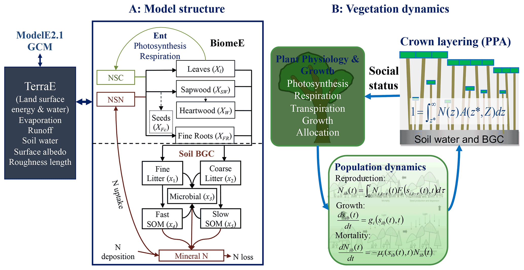
Figure 1 Schematic diagram of the coupling of BiomeE into ModelE. Panel (a) shows the structure of carbon and nitrogen pools and fluxes and the interactions of BiomeE with TerraE, the land surface model in ModelE. The lines are the flows of carbon (green), nitrogen (brown), and coupled carbon and nitrogen (black). The green box is for carbon only. The brown boxes are nitrogen pools. The black boxes are for both carbon and nitrogen pools. Panel (b) shows the processes of plant physiology, demography, and crown organization in BiomeE.

The Biome Ecological strategy simulator (BiomeE) is derived from the Geophysical Fluid Dynamics Laboratory's vegetation model, LM3-PPA (Weng et al., 2015, 2017, 2019). It simulates plant physiology, vegetation demography, adaptive dynamics (eco-evolutionary adaptation), and ecosystem carbon, nitrogen, and water cycles (Fig. 1). In this model, the PFTs are defined by a set of combined plant traits, with their values sampled from the observed ranges to represent a specific plant type. Individual plants are categorized into cohorts and arranged in different vertical canopy layers according to their height and crown area, following the rules of the perfect plasticity approximation model (PPA; Strigul et al., 2008). Sunlight is partitioned into canopy crown layers according to Beer's law (Beer, 1852; Swinehart, 1962). The cohort is the basic unit to carry out physiological and demographic activities, e.g., photosynthesis, respiration, growth, reproduction, mortality, and competition with other individuals.

The demographic processes generate and remove cohorts and change the size and density of plant individuals in the cohorts. With explicit the representation of cohort size and crown organization, the model simulates competition for light and soil resources, community assembly, and vegetation structural dynamics. These processes are hierarchically organized in this model and run at various time steps, namely half-hourly or hourly for plant physiology and soil organic matter decomposition, daily for growth and phenology, and yearly for demography.

For extending this model to the global scale, we designed a new set of PFTs to represent the functional diversity of global vegetation and a new phenological scheme to deal with temperature and water seasonality in coupling BiomeE into ModelE. Leaf photosynthesis processes are taken from ModelE's existing vegetation model, Ent (Kim et al., 2015), and used to calculate the carbon budget that drives vegetation dynamics. Plant growth, demographic processes, and soil organic matter decomposition and nitrogen cycle processes are from BiomeE (Fig. 1). The land surface energy and water fluxes are calculated by TerraE with land surface characteristics jointly defined by the vegetation model.

2.2 Plant functional types

In this model, we use a set of continuous plant traits to define plant functional types, so that the model is able to predict vegetation-emergent properties (such as dominant plant types, size structure, and compositional dynamics) in different climatic conditions based on the underlying plant physiological properties and ecological principles through eco-evolutionary modeling in the future. For example, life forms are defined by the continuums characterized by wood density (woody vs. herbaceous), height growth coefficient (tree vs. shrub), and leaf mass per unit area (LMA; for evergreen vs. deciduous). Deciduousness is defined by cold resistance (evergreen vs. cold deciduous) and drought resistance (evergreen vs. drought deciduous). Grasses are simulated as tree seedlings with all stems senescent along with leaves at the end of a growing season. The individuals are reset back to their initial sizes each year, and the population density is also reset by conserving current total biomass. The photosynthesis pathway is predefined as C₃ or C₄.

Table 1 Plant functional types used in BiomeE.

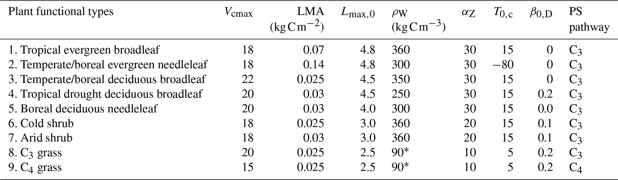
V_cmax is the leaf maximum carboxylation rate, LMA is the leaf mass per unit area, L_max,0 is the crown maximum leaf area index, ρ_W is the wood density, α_Z is the height coefficient, T_0,c is the critical temperature for phenology offset, β_0,D is the critical soil moisture index for the offset of phenology, and PS is the photosynthesis pathway. ^∗ Grass stem carbon density is calculated as tissue carbon divided by stem volume. The tissue density of the grass stems can be as high as wood.

We defined nine PFTs for our test runs in this paper to roughly represent global natural vegetation functional diversity (Table 1) according to their life form (tree, shrub, and grass), photosynthesis (C₃ and C₄), and leaf phenology (evergreen and deciduous). Crop PFTs were not included because the purpose of this paper is to describe the baseline processes of natural vegetation and soil biogeochemical cycle. These PFTs have the same physiological and demographical processes, with different parameters (except C₃ and C₄ photosynthesis pathways) representing varied strategies in different environments. Thus, for eco-evolutionary and ecological community assembly simulations, one PFT can switch to another by changing its parameters for searching competitively optimal plant traits in different environments.

2.3 Phenology

The phenology types are defined by two parameters, i.e., a critical low temperature and a critical soil moisture index, that are used to trigger leaf fall. These two parameters define four phenological types with their possible factorial combinations, i.e., evergreen, drought deciduous, cold deciduous, and drought–cold deciduous. Evergreen PFTs have high resistances to cold (i.e., very low critical temperature) and drought (very low soil drought). Cold and drought deciduous PFTs have low critical temperature and soil drought index, respectively. These phenological types represent different strategies of dealing with environmental stresses and the pressure of competition. It is possible that the evergreen would be more competitive in high seasonality regions (e.g., evergreen needleleaf trees in boreal regions), though the first response of plants to harsh environments (e.g., cold or dry) is to shed their leaves. Our definition of phenology is designed to allow the model to evaluate the competitively optimal strategy in future studies.

For the cold deciduous PFTs (temperate/boreal deciduous broadleaf and cold shrub), we use the growing degree days above 5 ^∘C (GDD₅) to trigger the phenological onset and a critical low temperature (T_m) for the offset. GDD₅ is calculated from the days that temperature starts to increase from the coldest days in the non-growing season. The critical GDD for a plant to initiate growth (GDD_c) is defined as a function of chilling days in the non-growing season, as follows (Prentice et al., 1992):

$$\begin{array}{}\text{(1)}& {\text{GDD}}_{\mathrm{c}}=a_{\mathrm{0}}+d\cdot e^{-b\cdot N_{\text{CD}}},\end{array}$$

where N_CD is the days of the cold period in non-growing season before bud burst, a₀ is the minimum GDD_c (50) when the cold period is sufficiently long, d is the maximum addition of GDD_c (800) when there is no cold period (i.e., N_CD=0), and b is a shape coefficient (0.025). These parameters are tunable and should change with the acclimation of plants to new climates.

The running mean temperature that represents the mean temperatures over a short period of time is calculated as follows:

$$\begin{array}{}\text{(2)}& \left\{\begin{array}{l}{T}_{\mathrm{m}}\left(i\right)=T_d\left(i\right),\text{ when }i=\mathrm{1}\\ T_{\mathrm{m}}\left(i\right)=\mathrm{0.8}{T}_{\mathrm{m}}(i-\mathrm{1})+\mathrm{0.2}{T}_d\left(i\right),\text{ when }i\ge \mathrm{2}.\end{array}\right.\end{array}$$

The critical temperature of triggering leaf senescence (T_c) is calculated as a function of the number of growing days (N_GD).

$$\begin{array}{}\text{(3)}& T_{\mathrm{c}}=T_{\mathrm{0},\mathrm{c}}-s\cdot e^{-c\cdot (max(\mathrm{0},N_{\text{GD}}-L_{\mathrm{0}}\left)\right)},\end{array}$$

where T_0,c is the highest critical temperature when N_GD is sufficiently long, s is the range that a critical temperature can change, c is a shape parameter, and L₀ defines the lowest critical temperature ($T_{\mathrm{0},\mathrm{c}}-s$) when N_GD is smaller than L₀. The rationale in this equation is that, when a growing period is not long enough, plants need a lower T_c to trigger leaf fall so that they can have a growing season that is not too short. This setting is based on the thermal adaptation analysis of Yuan et al. (2011). It balances the growing season length and frost risks by adjusting critical GDD_c and T_c according to chilling days and growing days to reduce the frost risk in warm regions and increase growing season length in cold regions. In this way, leaf senescence is also a function of growing season length and leaf aging. For example, in a region with a longer growing season, plants will have a higher T_c and initiate senescence when it is still relatively warm.

For the drought deciduous PFTs (tropical drought deciduous broadleaf, arid shrub, and C₄ grass), we used a soil moisture index (s_D) to start and end a growing season.

$$\begin{array}{}\text{(4)}& s_{\mathrm{D}}={\sum }_{i=\mathrm{1}}^n\text{Min}\left(\mathrm{1.0},\text{max}\left({\displaystyle \frac{{\mathit{\theta }}_i-{\mathit{\theta }}_{\text{WP},i}}{{\mathit{\theta }}_{\text{HC},i}-{\mathit{\theta }}_{\text{WP},i}}},\mathrm{0.0}\right)\right),\end{array}$$

where i is the soil layer in the root zone, θ is soil water content ($\text{vol.}/\text{vol.}$), θ_WP is the wilting point, and θ_HC is soil water holding capacity. The critical soil moisture values that trigger new leaf growth and leaf fall are defined as PFT-specific parameters. We slightly tuned these two parameters according to the soil moisture where the deciduous PFTs' leaves start to grow or fall. Usually, the critical soil moisture for starting new leaf growth is higher than the soil moisture that triggers leaf senescence so that the plants can have a stable growing season.

2.4 Plant allometry and demography

Allometry and plant architecture

The plant allometry and architecture are critical for plant resources allocation, light capture, and soil water and nutrients uptake. The allometry equations are the same as those used in LM3-PPA (Farrior et al., 2013; Weng et al., 2015):

$$\begin{array}{}\text{(5)}& \left\{\begin{array}{l}{A}_{\mathrm{C}}={\mathit{\alpha }}_{\mathrm{C}}{D}^{{\mathit{\theta }}_{\mathrm{C}}}\\ Z={\mathit{\alpha }}_{\mathrm{Z}}{D}^{{\mathit{\theta }}_{\mathrm{Z}}}\\ S=\mathrm{0.25}\mathit{\pi }\mathit{\rho }\mathrm{\Lambda }{\mathit{\alpha }}_{\mathrm{Z}}{D}^{\mathrm{2}+{\mathit{\theta }}_{\mathrm{Z}}}\\ A_{\mathrm{L}}^{\ast }=l_{\text{max}}{A}_{\mathrm{C}}\\ A_{\text{FR}}^{\ast }={\mathit{\phi }}_{\text{RL}}{l}_{\text{max}}{A}_{\mathrm{C}}\end{array}\right.,\end{array}$$

where D is tree diameter, A_C is crown area, Z is plant height, S is woody biomass (sapwood plus heartwood), and α_C and α_Z are the scaling factors for crown area and plant height, respectively. θ_C and θ_Z are the exponents for crown area and tree height, respectively, π is ratio of a circle's circumference to its diameter, ρ is wood density (kg C m⁻³), and Λ is the taper factor from a cylinder to a tree with the same D. $A_{\mathrm{L}}^{\ast }$ and $A_{\text{FR}}^{\ast }$ are the target surface area of leaves and fine roots, respectively, and φ_RL is the area ratio of leaves to roots. l_max is the maximum leaf area per unit crown area, which is defined as a function of plant height (Z) as follows:

$$\begin{array}{}\text{(6)}& l_{\text{max}}\left(Z\right)=L_{\text{max},\mathrm{0}}(Z+h_{\mathrm{0}})/(Z+H_{\mathrm{0}}),\end{array}$$

where L_max,0 is the maximum crown LAI when a tree is sufficiently tall, h₀ is a small number that makes a minimum l_max when the tree height is close to zero, and H₀ is a curvature parameter.

Plant growth and allocation of carbon and nitrogen to plant tissues

The allocation of carbon to wood, leaves, and roots is affected by climate and forest age (Litton et al., 2007; Xia et al., 2019). However, vegetation models cannot capture these patterns well at large spatial scales, even if the adaptive responses to climate and forest ages are considered (Xia et al., 2019, 2017), partly because of the absence of the explicit representation of shifts in species composition and competition between individuals (Franklin et al., 2012; Dybzinski et al., 2015). BiomeE has an optimal growth scheme that drives the allocation of carbon and nitrogen to leaves, fine roots, and stems based on the optimal use of resources and light competition (Weng et al., 2019). In this scheme, the growth of new leaves and fine roots follows the growth of woody biomass (i.e., stems), and the area ratio of fine roots to leaves is kept constant during the growing season. The allocation of available carbon between structural (e.g., stems) and functional (e.g., leaves and fine roots) tissues is optimal for light competition at given nitrogen availability.

Mathematically, differentiating the stem biomass allometry in Eq. (5) with respect to time, using the fact that $\mathrm{d}S/\mathrm{d}t$ equals the carbon allocated for wood growth (G_W), gives the following diameter growth equation:

$$\begin{array}{}\text{(7)}& {\displaystyle \frac{\mathrm{d}D}{\mathrm{d}t}}={\displaystyle \frac{G_{\mathrm{W}}}{\mathrm{0.25}\mathit{\pi }\mathrm{\Lambda }{\mathit{\rho }}_{\mathrm{W}}{\mathit{\alpha }}_{\mathrm{Z}}(\mathrm{2}+{\mathit{\theta }}_{\mathrm{Z}})D^{\mathrm{1}+{\mathit{\theta }}_{\mathrm{Z}}}}}.\end{array}$$

This equation transforms the carbon gain from photosynthesis to the diameter growth that results from wood allocation and allometry (Eq. 5). With an updated tree diameter, we can calculate the new tree height and crown area using allometry equations and the targets of leaf and fine root biomass (Eq. 5). Generally, the growing season average allocations of carbon and nitrogen to different tissues are governed by two parameters, namely the maximum leaf area per unit crown area (l_max) and fine root area per unit leaf area (φ_RL) (Eq. 5). The optimal growth allocation scheme combined with explicit competition for light and soil resources in our model makes it possible to simulate the underlying processes that determine emergent allocation patterns (Dybzinski et al., 2011; Farrior et al., 2013; Farrior, 2019; Weng et al., 2019).

Reproduction and mortality

At a yearly time step, the cumulative carbon and nitrogen allocated for reproduction by a canopy cohort over the growing season length, T, is converted to seedlings according to the initial plant biomass (S₀) and germination and establishment probabilities (p_g and p_e, respectively). Generally, the population dynamics can be described by a variant of the von Foerster (1959) equation:

$$\begin{array}{}\text{(8)}& \begin{array}{rl}& N(S_{\mathrm{0}},t)={\displaystyle \frac{p_{\mathrm{g}}{p}_{\mathrm{e}}}{S_{\mathrm{0}}}}{\int }_{\mathrm{0}}^{\mathrm{T}}N\left(\mathit{\tau }\right)G_{\mathrm{F}}\left(\mathit{\tau }\right)\mathrm{d}\mathit{\tau }\\ & {\displaystyle \frac{\mathrm{d}N(s,t)}{\mathrm{d}t}}=-\mathit{\mu }(s,t)N(s,t),\end{array}\end{array}$$

where N(S₀,t) is the spatial density of newly generated seedlings, N(τ) is the spatial density of this cohort of trees at time τ, G_F is the carbon allocation to seeds, and μ is PFT-specific mortality parameter.

Each PFT has a background mortality rate that is assigned from the literature. These background rates are assumed to be size-independent for the canopy layer trees but size-dependent for understory trees. Many factors affect tree mortality, such as light, size, competition crown damage, hydraulic failure, and trunk damage (Lu et al., 2021; Zuleta et al., 2022). These factors result in high mortality rates of seedlings and old trees (i.e., a U-shaped mortality curve). We use the following equation to delineate a mortality rate that varies with social status (crown layers), shade effects, and tree sizes:

$$\begin{array}{}\text{(9)}& \mathit{\mu }(s,t)={\mathit{\mu }}_{\mathrm{0}}(\mathrm{1}+f_{\mathrm{L}}{f}_{\mathrm{S}})f_{\mathrm{D}},\end{array}$$

where f_L is the shade effects on mortality ($f_{\mathrm{L}}=\sqrt{L-\mathrm{1}}$), f_S is seedling mortality when a tree is small ($f_{\mathrm{S}}=A_{\text{SD}}{e}^{-B_{\text{SD}}\cdot D}$), and f_D represents the size effect on the mortality of adult trees ($f_{\mathrm{D}}=m_{\mathrm{s}}\frac{e^{A_{\mathrm{D}}(D-D_{\mathrm{0}})}}{\mathrm{1}+e^{A_{\mathrm{D}}(D-D_{\mathrm{0}})}}$). L is the layer this plant is in (L=1 for the canopy layer, 2 for the second, and so on), A_SD is the maximum multiplier of mortality rate for the seedlings in the understory layers, B_SD is the rate of mortality decreasing as tree diameter (D) increases, m_s is the maximum multiplier of mortality rate for large-sized trees, D₀ is the diameter at which the mortality rate increases by $m_{\mathrm{s}}/\mathrm{2}$, and A_D is a shape parameter (i.e., the sensitivity to tree diameter).

2.5 Crown self-organization and layering

Tree crowns are arranged into different vertical canopy layers according to tree height and crown area if their total crown area is greater than the land area following the rules of the PPA model (Strigul et al., 2008). In PPA, individual tree height is defined as the height at the top of the crown, and all leaves of a given cohort are assumed to belong to a single canopy layer. The height of canopy closure for the top layer is referred to as the critical height (Z^∗; the height of the shortest tree in the layer) and is defined implicitly by the following equation:

$$\begin{array}{}\text{(10)}& k(\mathrm{1}-\mathit{\eta })={\sum }_i{\int }_{Z^{\ast }}^{\mathrm{\infty }}{N}_i(Z,t)A_{\text{CR},i}(Z^{\ast },Z)\mathrm{d}Z,\end{array}$$

where N_i(Zt) is the density of PFT i trees of height Z per unit ground area, $A_{\text{CR},i}\left(Z^{\ast }Z\right)$ is the crown area of an individual PFT i tree of height Z, η is the proportion of each canopy layer that remains open on average due to wind and imperfect spacing between individual tree crowns, and k is the ground area. The top layer includes the tallest cohorts of trees whose collective crown area sums to 1−η times the ground area, and lower layers are similarly defined.

All the trees taller than the critical height can receive full sunlight, and all trees below this height are shaded by the upper-layer trees. Trees within the same layer do not shade each other, but there is self-shading among the leaves within individual crowns. Cohorts in a sub-canopy layer are shaded by the leaves of all taller canopy layers. In each canopy layer, all cohorts are assumed to have the same incident radiation on the top of their crowns. Note that the gap fraction η is necessary to allow additional light penetration through each canopy layer for the persistence of understory trees in monoculture forests in which the upper-layer crowns build a physiologically optimal number of leaf layers (Farrior et al., 2013). The grasses only form one layer. Those individuals who cannot stay in that layer because of limited space will be killed (i.e., when the total grass crown area is larger than the land area).

2.6 Ecosystem carbon and nitrogen biogeochemical cycles

There are seven pools in each plant, i.e., leaves, fine roots, sapwood, heartwood, fecundity (seeds), and non-structural carbohydrates and nitrogen (NSC and NSN, respectively). The carbon and nitrogen in the plant pools enter the soil pools with the mortality of individual trees and the turnover of leaves and fine roots. Soil has a mineral nitrogen pool for mineralized nitrogen and five soil organic matter (SOM) pools for carbon and nitrogen, with metabolic litter (x₁), structural litter (x₂), microbial (x₃), and fast- (x₄) and slow-turnover (x₅) SOM pools.

The decomposition processes are simulated by a model modified from Manzoni et al. (2010). It was described in Weng et al. (2019, 2017). The decomposition rate of a SOM pool is determined by the basal turnover rate together with soil temperature and moisture, following the formulation of the CENTURY model (Parton et al., 1988, 1987). The microbial pool transfers carbon and nitrogen among SOM pools and releases mineralized nitrogen. Microbial carbon use efficiency (CUE; carbon transfer from litter to microbial matter) is a function of litter nitrogen content, following the model of Manzoni et al. (2010).

The N mineralization in decomposition is determined by microbial nitrogen demand, which is the SOM C:N ratio, and decomposition rate. In the high C:N ratio SOM, microbes must consume excess carbon to obtain enough nitrogen for growth. By contrast, in the low C:N ratio SOM, microbes must release excess nitrogen to obtain enough carbon for energy. Depending on the C:N ratios of SOM, soil microbes may be limited by either C or N.

The out-fluxes of C and N from the ith pool (dC_i and dN_i, respectively) are calculated by the following:

$$\begin{array}{}\text{(11)}& \begin{array}{rl}& \mathrm{d}{C}_i=\mathit{\xi }(T,\mathit{\theta }){\mathit{\rho }}_i{\mathrm{QC}}_i,\\ & \mathrm{d}{N}_i=\mathit{\xi }(T,\mathit{\theta }){\mathit{\rho }}_i{\mathrm{QN}}_i,\end{array}\end{array}$$

where ξ is the response function of decomposition to soil temperature (T) and moisture (θ), ρ_i is the basal turnover rate of the ith litter pool at reference temperature and moisture, QC_i is the C content in ith pool, and QN_i is the N content in the ith pool.

The microbial growth (dM) is calculated as the co-limit of available carbon and nitrogen mobilized at this step:

$$\begin{array}{}\text{(12)}& \mathrm{d}{M}_i=\text{Min}({\mathit{\epsilon }}_{\mathrm{0}}\cdot \mathrm{d}{C}_i,{\mathrm{\Lambda }}_{\text{microbe}}\cdot \mathrm{d}{N}_i),\end{array}$$

where ε₀ is default carbon use efficiency of the litter decomposition (0.4), and Λ_microbe is a microbe's C:N ratio, which is a fixed value (10 in this model). The soil heterotrophic respiration (R_h) is the microbial respiration (i.e., the difference between carbon consumption and new microbial growth), and the total N mineralization rate (N_mineralized) is calculated as the sum of mineralized N in the SOM pools and microbial turnover, as follows:

$$\begin{array}{}\text{(13)}& \begin{array}{rl}& R_{\mathrm{h}}={\sum }_{i=\mathrm{3}}^{\mathrm{5}}\mathrm{d}{C}_i-{\sum }_{i=\mathrm{4}}^{\mathrm{5}}{m}_i,\\ & {\mathrm{N}}_{\mathrm{mineralized}}={\sum }_{i=\mathrm{3}}^{\mathrm{5}}\mathrm{d}{N}_i-{\sum }_{i=\mathrm{3}}^{\mathrm{5}}{m}_i/{\mathrm{\Lambda }}_{\text{microbe}}.\end{array}\end{array}$$

The R_h releases to atmosphere as CO₂. Mineralized N enters the mineral N pool for plants to use. The dynamics of the mineral N pool is represented by the following equation:

$$\begin{array}{}\text{(14)}& {\displaystyle \frac{\mathrm{d}{\mathrm{N}}_{\text{mineral}}}{\mathrm{d}t}}={\mathrm{N}}_{\mathrm{deposition}}+{\mathrm{N}}_{\mathrm{mineralized}}-U-{\mathrm{N}}_{\mathrm{loss}},\end{array}$$

where N_deposition is the N deposition rate, assumed to be constant over the period of simulation, N_m is the N mineralization rate of the litter pools (fast and slow SOM and microbes), U is the N uptake rate ($\mathrm{kg}\mathrm{N}{\mathrm{m}}^{-\mathrm{2}}{\mathrm{h}}^{-\mathrm{1}}$) of plant roots, and N_loss includes the loss of mineralized N by denitrification and runoff. The N deposition (N_deposition) is the only N input to ecosystems, and we set nitrogen fixation as zero in this version of the model.

3 Model test

For our comparison of the model performance against observations and other models, we used the full demographic version of BiomeE (described above) and also designed a single-cohort version of the model to benchmark our demographic implementations. In the single-cohort model, the mortality of trees is simulated as the turnover of woody biomass, and the fecundity resources (carbon and nitrogen) are used to build the same-sized parent trees, instead of seedlings growing from understory layers. If the total crown area of the trees in this cohort is greater than the land area, then the extra trees will be removed to make the total crown area less than or equal to the land area. At equilibrium, the turnover of woody biomass is equal to the new growth each year, and the new trees generated from fecundity resources are killed by self-thinning. The single-cohort model uses the mean state of the canopy layer trees to represent the characteristics of the whole community. This single-cohort model performs like the traditional biogeochemical models and simplifies vegetation computation.

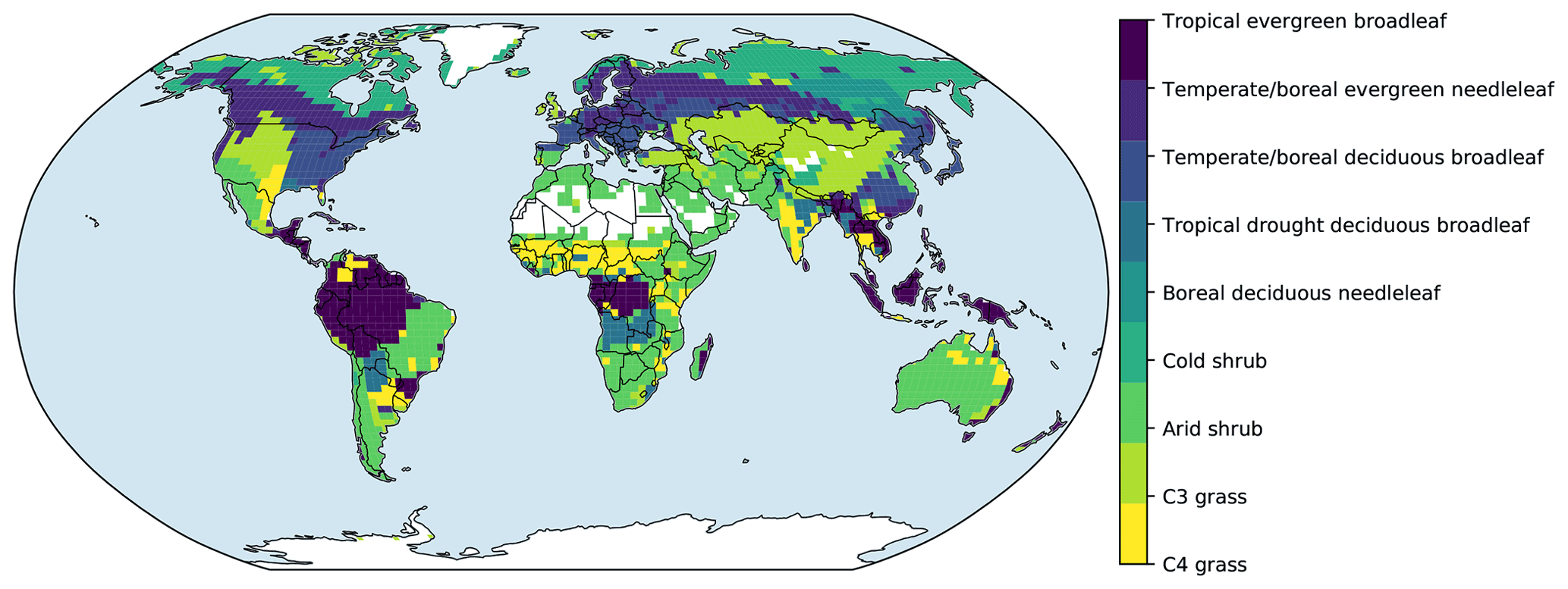
Figure 2 Prescribed global distribution of plant functional types. Data are from the Ent global vegetation structure map.

In the test runs, the distribution of PFTs was obtained from the Ent vegetation map (Ito et al., 2020), which was derived from 2004 MODIS land cover and PFT data products (Friedl et al., 2010) and climate data (Fig. 2). For these simulations, croplands and pastures were replaced by the potential natural vegetation types. We slightly tuned the leaf maximum carboxylation rate (V_cmax) to fit the general pattern of global gross primary productivity (GPP), while keeping other parameters unchanged.

Forcing data are from the TRENDY project CRU-NCEP data (Sitch et al., 2015) and have a 6 h time step at a spatial resolution of 0.5^∘ × 0.5^∘. These data are available at https://www.uea.ac.uk/web/groups-and-centres/climatic-research-unit/data (last access: 27 October 2022).

We aggregated these data into 2.0^∘ × 2.5^∘ grid cells and used 30 years of data (1988–2017) to force the model to run for 600 years, which is long enough for the model to approach equilibrium states for both vegetation and soil carbon pools. These data include temperature, precipitation, shortwave radiation, longwave radiation, specific humidity, and wind speed (U and V directions). We interpolated the radiation data (R_S) into half-hour time steps based on the sun zenith angle (θ_S) and the radiation penetration rate calculated from the data.

$$\begin{array}{}\text{(15)}& R_{\mathrm{S}}\left(t\right)=\left({\displaystyle \frac{R_{\text{H6}}}{S^{\ast }\text{cos}{\mathit{\theta }}_{\mathrm{S}}\left(\text{H6}\right)}}\right)S^{\ast }\text{cos}{\mathit{\theta }}_{\mathrm{S}}\left(t\right),\end{array}$$

where S^∗ is solar constant (1362 W m⁻²). Other variables are linearly interpolated to the model run time step, which is a half-hour in this study. Atmospheric CO₂ concentration is set at the model default level (350 ppm; parts per million).

3.1 Data sources for model evaluation

The LAI data were from the Ent vegetation dataset (Ito et al., 2020), where the LAI was derived from 2004 MODIS LAI data (Tian et al., 2003, 2002). Gross primary productivity (GPP) data are from a global retrieval of GPP, using remote sensing observations. These data are on a 1^∘ × 1^∘ geographic grid at a monthly time step, based on an artificial neural network retrieval algorithm (Alemohammad et al., 2017). This algorithm uses six remotely sensed observations as input, i.e., solar-induced fluorescence (SIF), air temperature, precipitation, net radiation, soil moisture, and snow water equivalent. The data are available from 2007 to 2015. The tree height data are from spaceborne light detection and ranging (lidar) global map of canopy height at 1 km spatial resolution, as developed by Simard et al. (2011). These authors used the 2005 data from the Geoscience Laser Altimeter System (GLAS) aboard ICESat (Ice, Cloud, and land Elevation Satellite) to derive global forest canopy heights. Biomass data are from Global 1^∘ Maps of Forest Area, Carbon Stocks, and Biomass, 1950–2010 developed by Hengeveld et al. (2015). Soil carbon data are from the Food and Agriculture Organization (FAO) Harmonized World Soil Database (version 1.2), updated by Wieder et al. (2014).

MsTMIP model simulation data

We selected six model simulations (BiomeBGC, CTEM, CLM4, LPJ, ORCHIDEE, and VEGAS) from the Multi-scale Synthesis and Terrestrial Model Intercomparison Project (MsTMIP; Huntzinger et al., 2013) to compare against our model simulations. These models are well-developed and widely used in Earth system models, representing the state-of-art of current land vegetation model development. MsTMIP provided prescribed land use types for all participant models. However, it is up to the participant models to simulate disturbance impacts on ecosystems (Huntzinger et al., 2013). MsTMIP conducted five sets of experimental runs with different climate forcing, land use history, atmospheric CO₂ concentration, and nitrogen deposition. In this study, we compared to the SG1 simulation experiment because it is driven by the 1901–2010 climate forcing data with constant CO₂ concentration and constant land cover (Huntzinger et al., 2013), which are the closest to our model runs.

Table 2 Sites for simulated ecosystem development illustration.

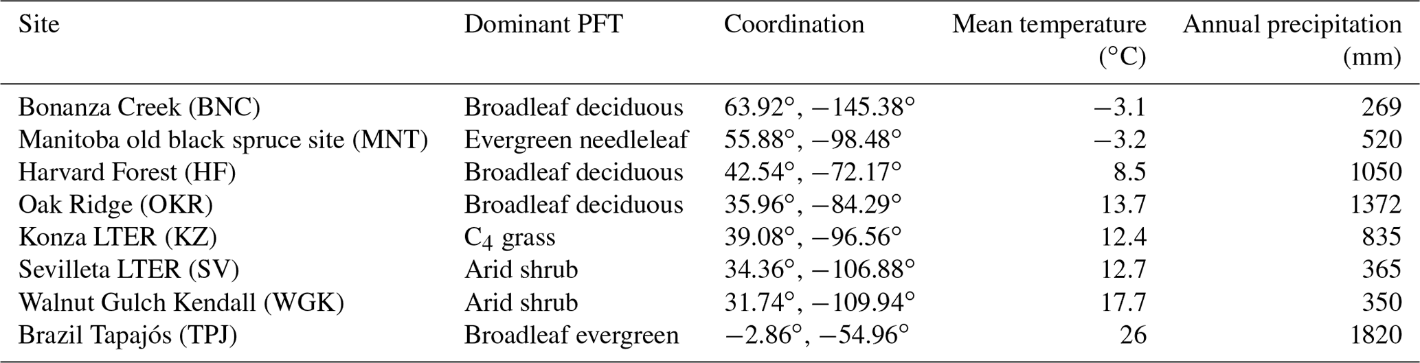
3.2 Selected grid cells for comparison

To illustrate model behavior, we selected eight grid cells that cover boreal forests, temperate forests, tropical forests, C₄ grasslands, and arid shrublands to show the simulated ecosystem development patterns across the climate zones with different dominant PFTs (Table 2). Brazil Tapajós (TPJ), Oak Ridge (OKR), Harvard Forest (HF), Manitoba old black spruce site (MNT), and Bonanza Creek (BNC) are covered by tree PFTs. The Konza long-term ecological research station (LTER; KZ) is C₄ grass. Walnut Gulch Kendall (WGK) and Sevilleta LTER (SV) are covered by arid shrubs. These sites were chosen because they have extensive data on vegetation and climate conditions for future comparisons.

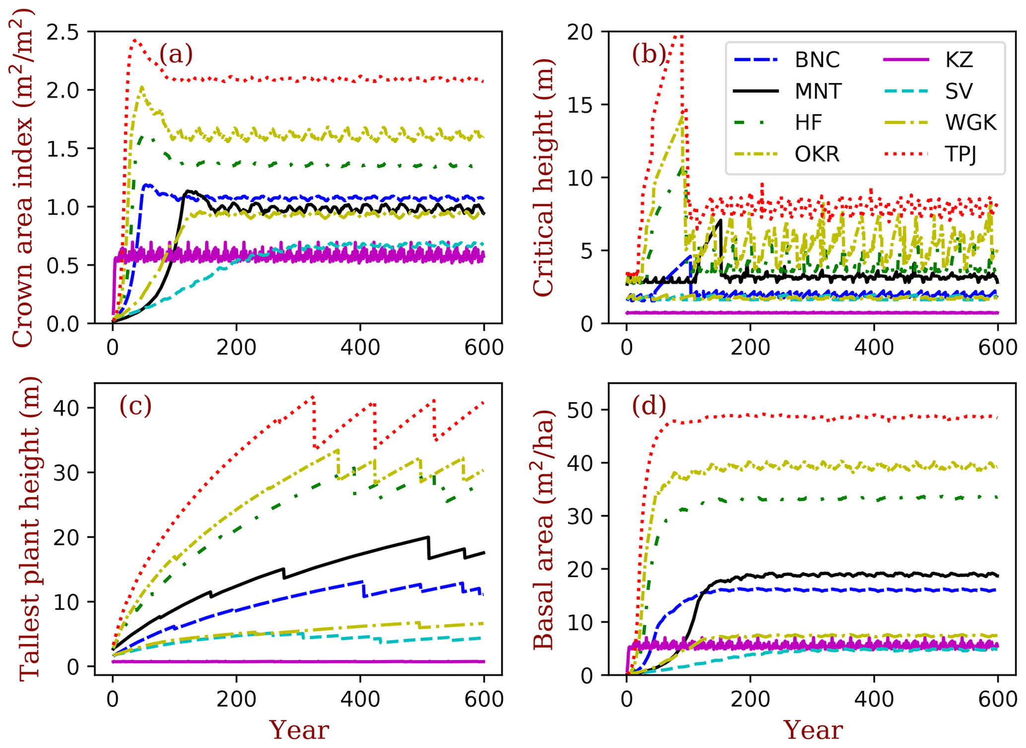
Figure 3 Vegetation structural dynamics with the full demographic BiomeE at the field sites listed in Table 2. Critical height (b) is an index of the model PPA, which separates the trees that are in full sunlight if taller than critical height and those that are fully shaded if shorter than critical height.

4 Results

4.1 Simulated vegetation structural and ecosystem carbon dynamics

In the forest sites, the simulated vegetation structure by the full demographic model changes with the growth, regeneration, and mortality processes (Fig. 3). The temporal dynamics of the canopy development can be separated into three stages according to the following canopy crown dynamics: (1) open forest stage, (2) self-thinning stage, and (3) stabilizing stage.

In the open forest stage, the crown area index (CAI) is less than 1.0, and all the individuals are in full sunlight. The tree crowns grow rapidly to occupy the open space (Fig. 3: a). In the self-thinning stage, the open space is filled by the crowns of similar sized trees (i.e., the forest is closed), canopy trees are continuously pushed to the lower layer(s) (i.e., self-thinning), and the CAI continues to increase due to the limited space with growing tree crowns (i.e., the new spaces vacated from the canopy tree mortality cannot meet the space demand from crown growth). The sizes of trees in the canopy layer are still similar (Fig. 3b and c), and the critical height (the shortest tree height in top layer) keeps increasing in this period.

In the stabilizing stage, when the space generated by the mortality of canopy trees is larger than the growth of canopy tree crown area, no trees are pushed to the lower layer, and the lower-layer trees start to enter the canopy layer, leading to a sharp decrease in critical height (Fig. 3b) and the mixing of different sized trees in the canopy layer. The CAI is decreasing as well because of the high mortality rates of the understory layer trees. The growth, regeneration, mortality, and space-filling processes are eventually equilibrated with model run, and the forest structure is then stabilized.

The tallest plant height (Fig. 3c), the height the tallest cohort, keeps increasing as this cohort exists. The sharp decrease indicates a replacement by or merging with another shorter cohort because the density of trees in this cohort is low (1.0 ha⁻¹ in this case), or the similarity between the tallest and the second tallest is high. The total basal area (Fig. 3d) is an index of the sum of all trees at a site. It keeps increasing during forest development and is equilibrated earlier than height and crown structure.

In these sites, at equilibrium, the tropical forest site (TPJ) has the highest crown area index (around 2.2), followed by warm temperate forest at OKR, mixed forest at HF, and boreal forests at BNC and MNT (Fig. 3). The shrubs and grasslands in arid regions have the lowest crown area index (CAI), with the basal area following similar patterns. For forested sites, tree height is tallest at TPJ, followed by OKR, HF, MNT, and BNC. The shrubs are short, according to their allometry parameters, and the height of grasses during non-growing season is zero. The critical height, which separates canopy layer trees from the understory layers, follows the same order as that of tree height with high fluctuations with cohort changes. (More cohort details are shown in Figs. S1–S8 in the Supplement)

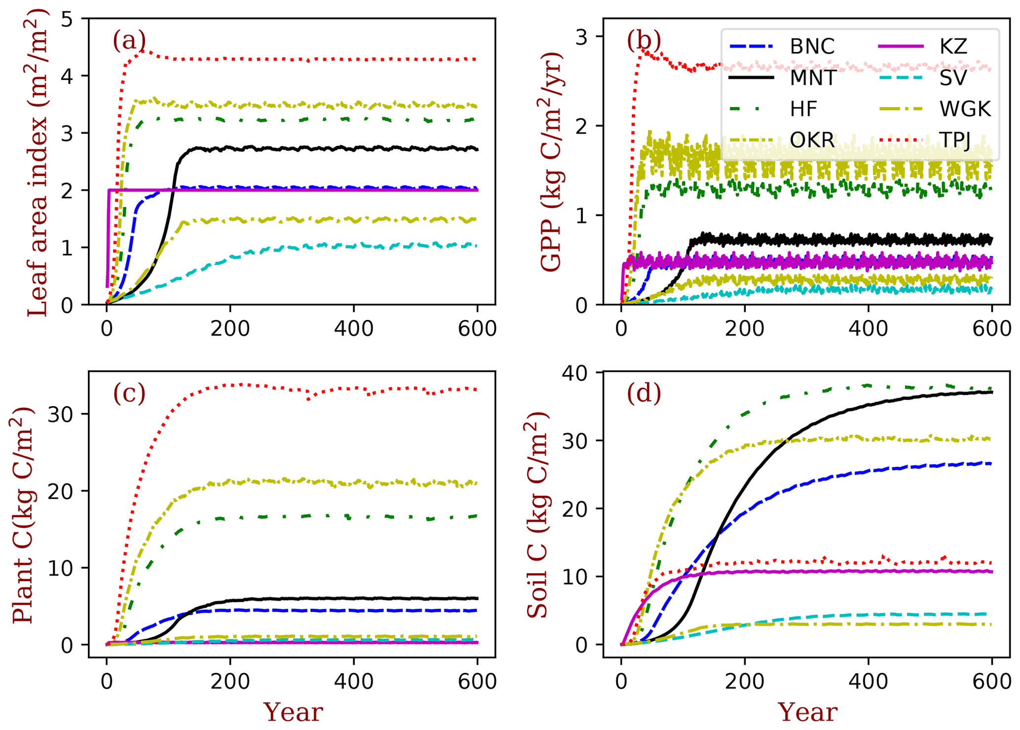
Figure 4 Site ecosystem development simulated by BiomeE with full demography for the field sites listed in Table 2. GPP is the gross primary production ($\mathrm{kg}\mathrm{C}{\mathrm{m}}^{-\mathrm{2}}{\mathrm{yr}}^{-\mathrm{1}}$), plant C is the vegetation biomass (kg C m⁻²), and soil C is the soil organic matter (kg C m⁻²).

For the temporal dynamics in the full demographic simulation (Fig. 4), the simulated GPP aligns closely with LAI, and they reach their equilibrium states at similar times across sites (Fig. 4a and b). According to the definition of maximum crown LAI (l_max) in Eq. (6), the grass LAI (i.e., Konza) reaches the maximum each year, except for the first year, due to the low initial density (Fig. 4a). The biomass accumulation is much slower in forests because of the longer time needed for forest structure (size distribution) to reach equilibrium. Soil carbon equilibration is faster in the warm regions than in cold regions overall because of the higher turnover rate of SOM pools in warm regions. At equilibrium, forested sites have higher LAI, biomass, and carbon stocks per area compared to the shrub and grass sites overall. Vegetation biomass is lowest at the grassland site, Konza LTER, because, within the model, the grassland ecosystems cannot accumulate persistent biomass.

The PFTs at TPJ and MNT are evergreen trees. Their LAI does not change over the whole year (Fig. 5a). The forest in OKR has the longest growing season in the three deciduous forest grids, followed by HF and BNC. BNC's growing season is only around 120 d, which is about half of OKR's growing season. The growing season of grasses in KZ starts in late May and ends in September. The two arid-adapted shrub sites (SV and WGK) are controlled by water availability. In TPJ (tropical evergreen forest), the trees have photosynthesis throughout the entire year (Fig. 5b). In MNT, photosynthesis only happens in warm seasons with the leaves kept in the crowns because of the dominant PFT is evergreen needleleaf tree. The deciduous trees in OKR and HF have high photosynthesis rates during the growing season. The photosynthesis rates in SV and WGK are generally low because of the dry environments. However, the precipitation events can drive photosynthesis rates high in these arid regions.

Figure 5 Seasonal patterns of LAI and gross primary production (GPP) in the sample grids. In total, 2 years of data are shown in this figure. The key to the location abbreviations is given in Table 2.

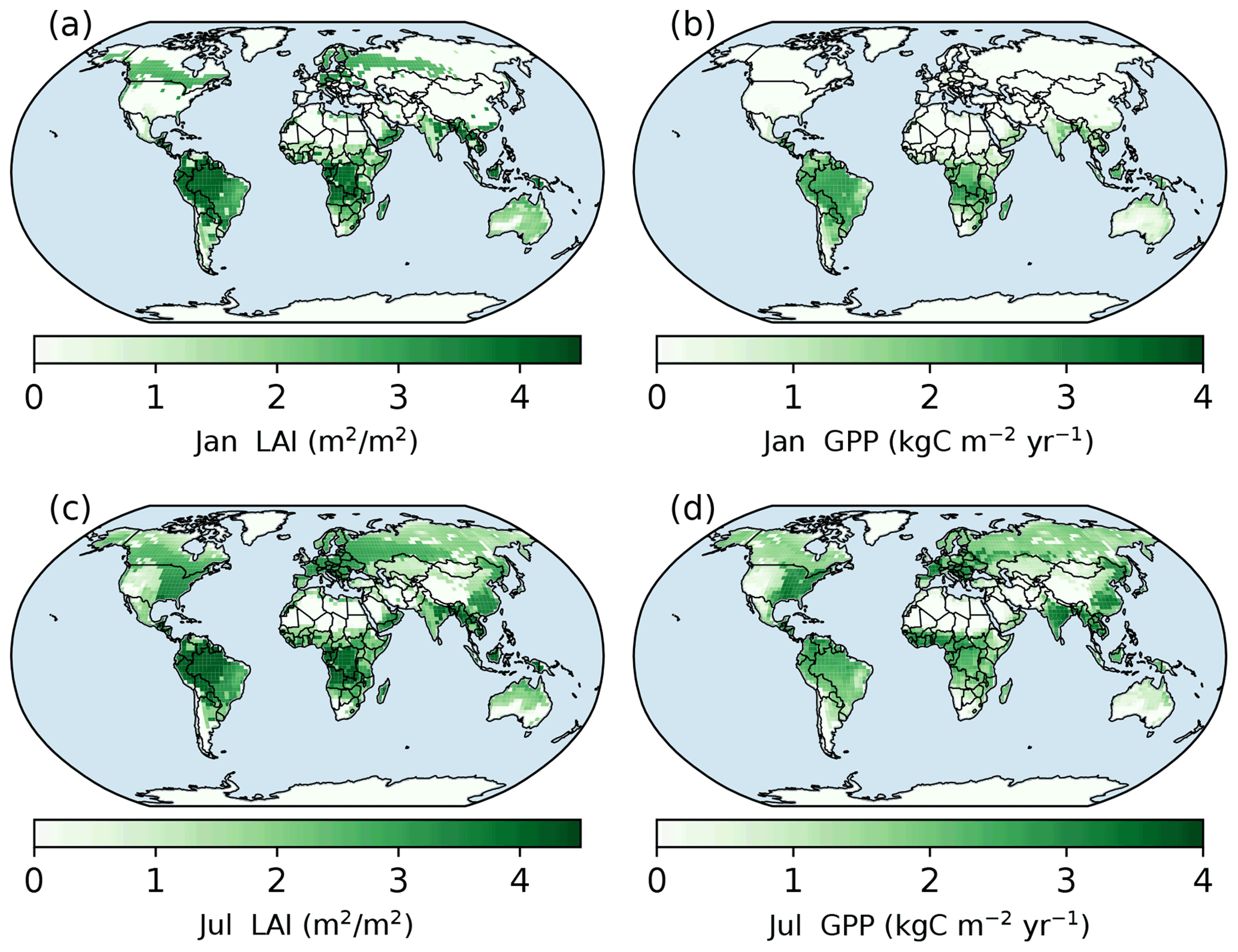
Figure 6 Spatial patterns of LAI and gross primary production (GPP) in January and July simulated with the full demography model setting. Panels (a) and (b) are the LAI and GPP of January in the year of 600 (the last year of model run). Panels (c) and (d) are the LAI and GPP of July in the same year.

As shown in Fig. 6a, the evergreen needleleaf forests keep their leaves in northern high-latitude regions during January, while the photosynthesis rate in this region is low (Fig. 6b). In July, northern high-latitude regions green up, and their photosynthesis rates are high in wet regions. The single-cohort model run predicts a similar pattern because of the same phenology model (Fig. S9).

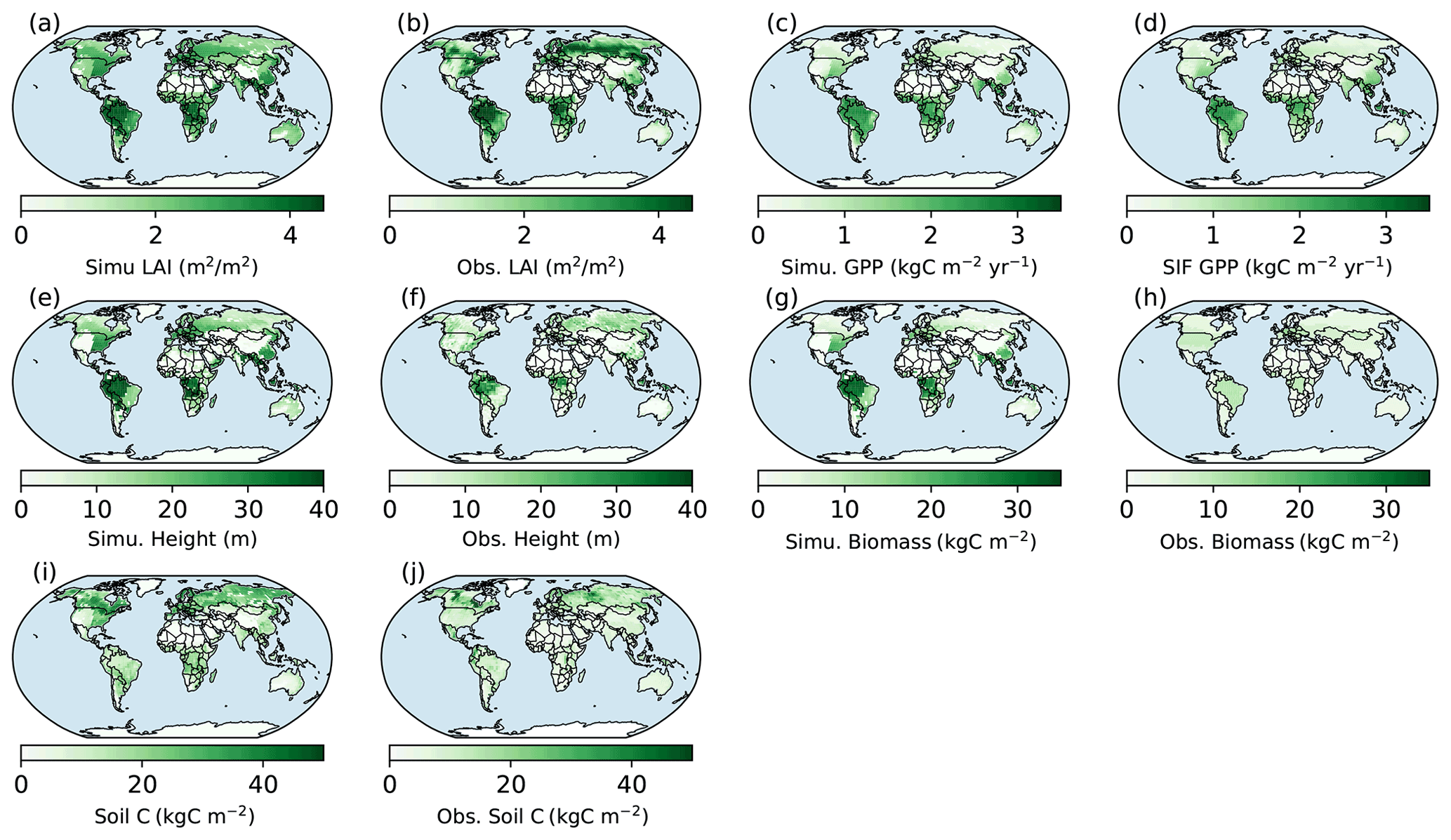
Figure 7 Spatial patterns of BiomeE (full demography) simulations and those from data. Obs. means different ways retrieved from observations. Obs. LAI is from Ent vegetation data (MODIS LAI 2004; Ito et al., 2020; Tian et al., 2003). Obs. GPP is derived from solar-induced fluorescence (SIF) data with a machine learning approach (Alemohammad et al., 2017). The data are available from January 2007 to December 2015. The tree height data are from spaceborne light detection and a ranging (lidar) global map of canopy height at 1 km spatial resolution, as developed by Simard et al. (2011). Biomass data are from Hengeveld et al. (2015). Soil carbon data are from the FAO Harmonized World Soil Database (version 1.2), which was updated by Wieder (2014).

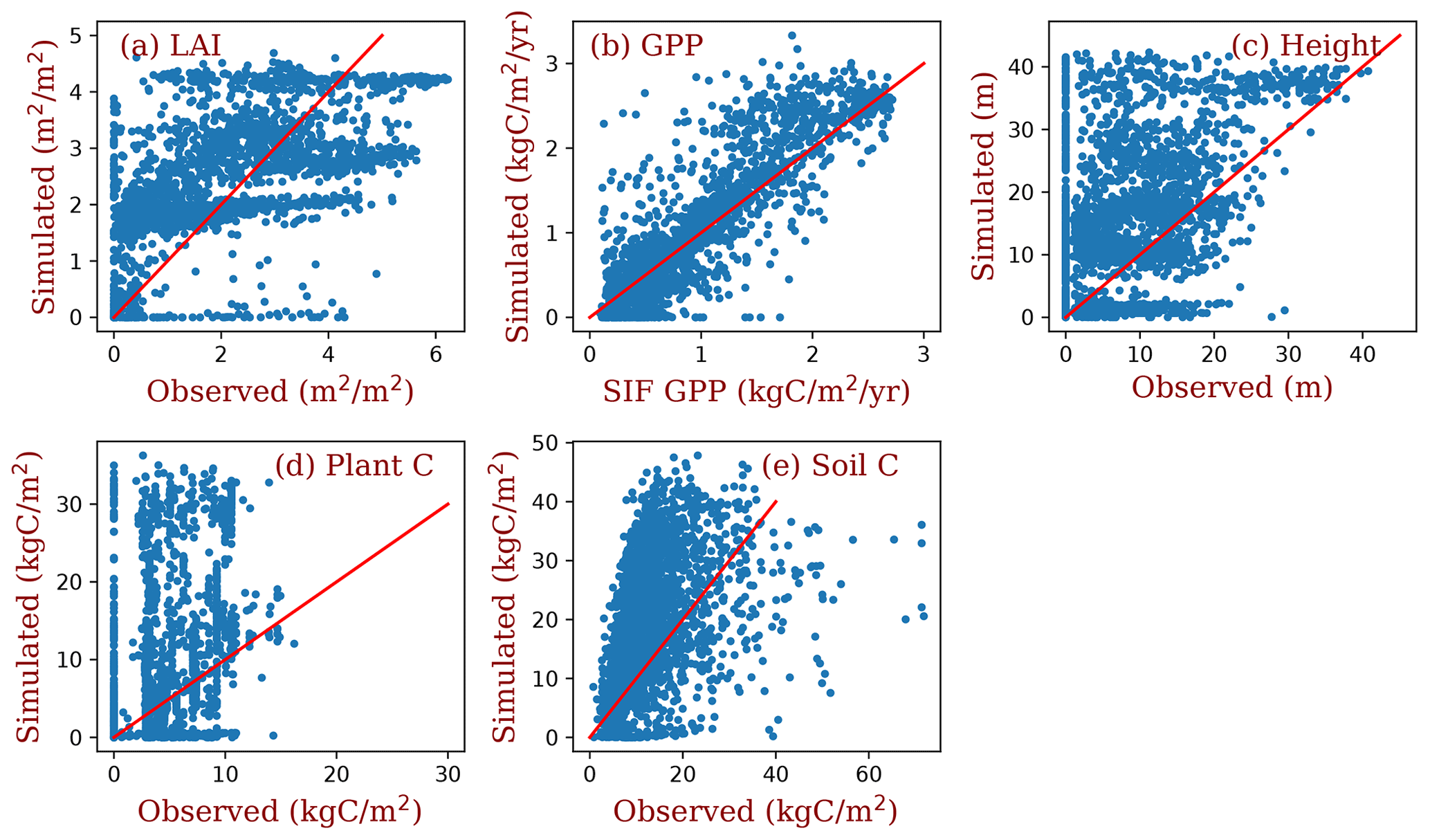
Figure 8 Grid comparison of full demographic BiomeE simulations with observations estimates. The red line in each panel is the 1:1 line. The data used in this figure are the same as those in Fig. 7.

4.2 Global comparisons with observations

The simulated LAI roughly captures the spatial pattern of MODIS LAI (Fig. 7a and b), though there are high variations at each grid (Fig. 8a). Generally, the simulated LAI in well-vegetated grids, e.g., boreal forest regions, is underestimated by our model because the crown LAI is calculated as a function of tree height and a parameter of maximum crown LAI (Table 1 and Eq. 6). The LAI in the grids that were converted to different land use types is overestimated because we assume all terrestrial grids are covered by potential vegetation in our test runs.

Compared with the SIF GPP (Alemohammad et al., 2017), simulated GPP is higher than the SIF GPP generally, though lower in arid regions (Figs. 7c, d and 8b). The simulated tree height (Figs. 7e, f and 8c) is mostly taller compared to observations (Simard et al., 2011) because most forests have been altered by human activities (Pan et al., 2013). However, the simulations and observations cover approximately the same range of tree heights (up to 40 m). Simulated biomass is much higher than the observations (Figs. 7g, h and 8d) because, in the observations, many forest regions have been transformed to low biomass land use types (such as croplands) or represent earlier successional stages with less accumulated carbon (i.e., not equilibrium states).

Simulated soil carbon does track the observations (Figs. 7i, j and 8e) better than biomass, likely because soil carbon stocks are more stable compared to biomass in response to disturbances and human activities. For areas where the model underpredicts soil carbon, the difference could arise from the missing biogeochemical processes that may lead to high carbon accumulation in some regions (e.g., peat; Davidson and Janssens, 2006; Briones et al., 2014; Euskirchen et al., 2014) and relatively high uncertainties in the soil carbon data (Tifafi et al., 2018).

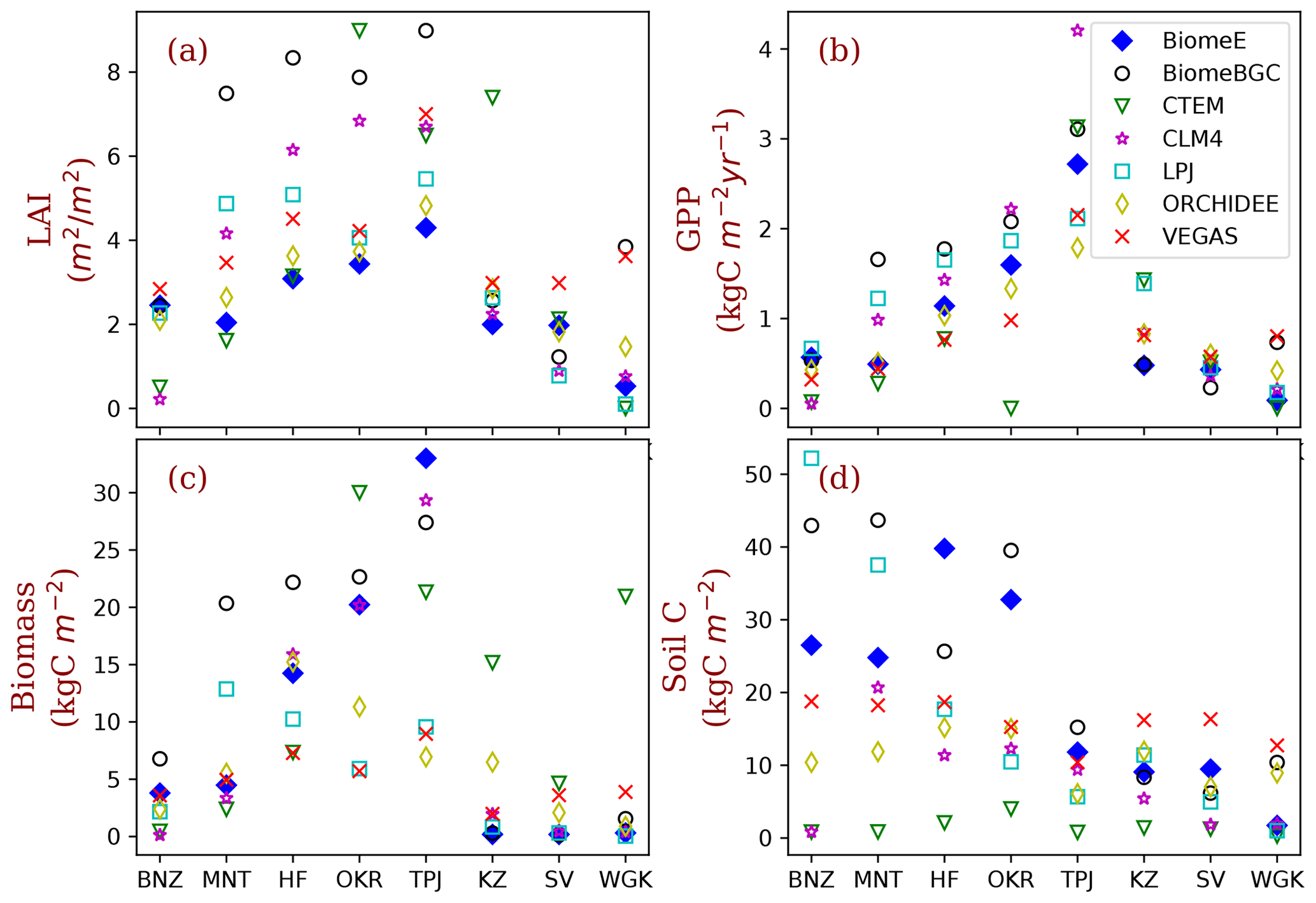
Figure 9 Site-level comparison with MsTMIP models. The BiomeE predictions are from the full demography. The abbreviations of the eight sites (corresponding to model grid cells) and their coordination, dominant PFTs, and climatic conditions are given in Table 2. (See Fig. S12 in the Supplement for the single-cohort BiomeE simulations).

4.3 Comparison with MsTMIP models

We compared the performance of our model with MsTMIP models at the eight locations that were used to show ecosystem development patterns (Table 2). For most of these sites, LAI in BiomeE is lower compared the other MsTMIP models (Fig. 9a), while the estimated GPP is within the range of MsTMIP predictions (Fig. 9b). LAI differences are a consequence of the formulations within BiomeE, as described further in Sect. 5.2. Specifically, BiomeE simulates leaf growth by using a maximum crown LAI, which is lower than the real forest LAI.

The low LAI does not affect crown total photosynthesis because leaves in lower canopy layers contribute little to the total carbon assimilation. BiomeE-predicted biomass (Fig. 9c) and soil carbon (Fig. 9d) generally fall towards the higher end of the MsTMIP simulations, except for the more arid grass- and shrub-dominated sites. We note, however, that there are wide-ranging differences in estimates for vegetation and soil carbon across the models, likely because of different treatments of mortality and decomposition functions in these models.

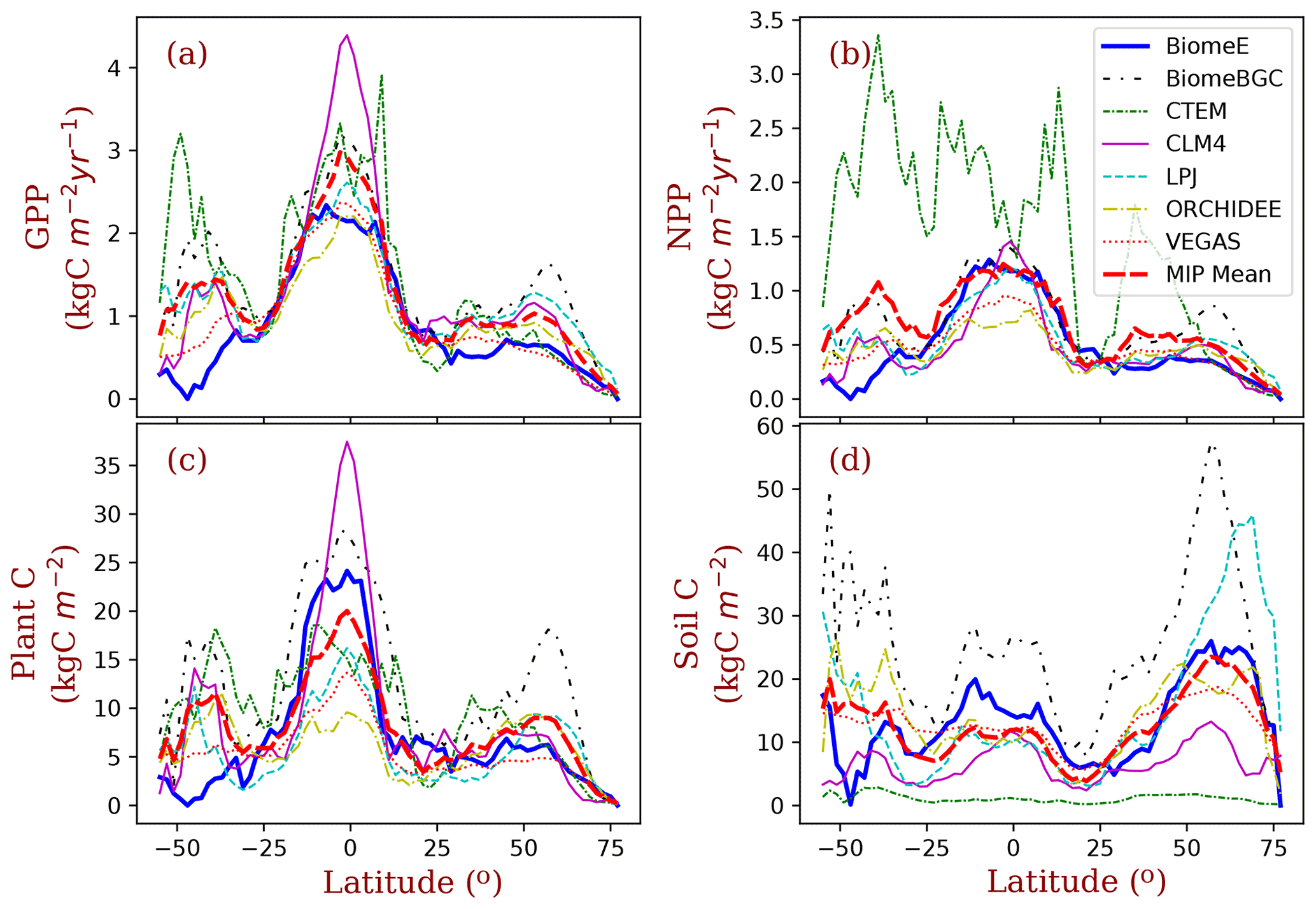
Figure 10 Latitudinal patterns of GPP, NPP, biomass, and soil carbon, as simulated by the BiomeE (with full demography) and MsTMIP models. The MIP Mean is the mean of the six MsTMIP model simulations. (See Fig. S13 in Supplement for the single-cohort BiomeE simulations).

More broadly, the latitudinal mean of BiomeE simulated GPP is at the lower end of MsTMIP model predictions (Fig. 10a). Since the BiomeE GPP was tuned to fit remote sensing data-derived GPP, the MsTMIP models may overestimate global GPP. The net primary production (NPP; Fig. 10b), plant carbon (Fig. 10c), and soil carbon (Fig. 10d) simulated by BiomeE are within the range simulated by the MsTMIP models. This indicates that BiomeE has a slightly lower respiration than the MsTMIP models. In the arid regions (e.g., around latitude 40–50^∘ S of South America), we simulated a lower GPP than that of MsTMIP models because of high drought sensitivity in our model.

The demographic processes have significant impacts on the simulated GPP, biomass, soil carbon, and vegetation structure compared to the single-cohort BiomeE (Fig. 11). The full demographic BiomeE includes an understory layer of plants, resulting in higher LAI in high LAI regions and also slightly higher GPP. However, the total biomass predicted by the two model settings are similar because of the tradeoffs in the allocation between leaves and stem growth and tree size distribution and because most biomass is in woody tissues (see Figs. S10 and S11 in the Supplement for the single-cohort BiomeE simulations). In the full demography model, tree mortality removes all the biomass, including leaves, fine roots, and stems, while in the single-cohort model, the mortality is represented as the turnover of woody biomass. Consequently, the full demography model has a higher emergent turnover rate for the whole vegetation carbon pool.

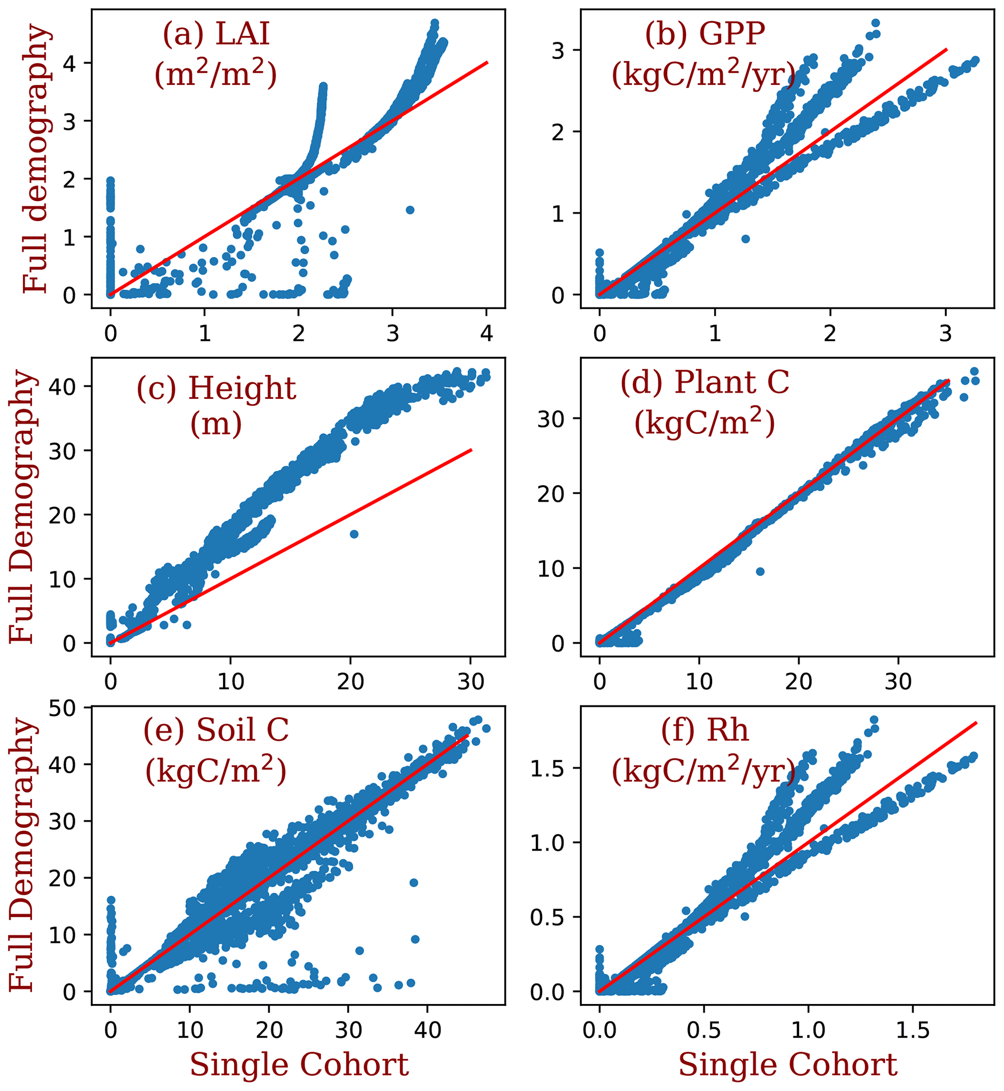
Figure 11 Comparison between the simulations of the full demography and the single-cohort settings of BiomeE. LAI is the leaf area index, GPP is the gross primary production (kg C m² yr⁻¹), height is the maximum tree height, plant C is the vegetation biomass (kg C m⁻²), soil C is the soil organic matter (kg C m⁻²), and R_h is the heterotrophic respiration rate ($\mathrm{kg}\mathrm{C}{\mathrm{m}}^{-\mathrm{2}}{\mathrm{yr}}^{-\mathrm{1}}$).

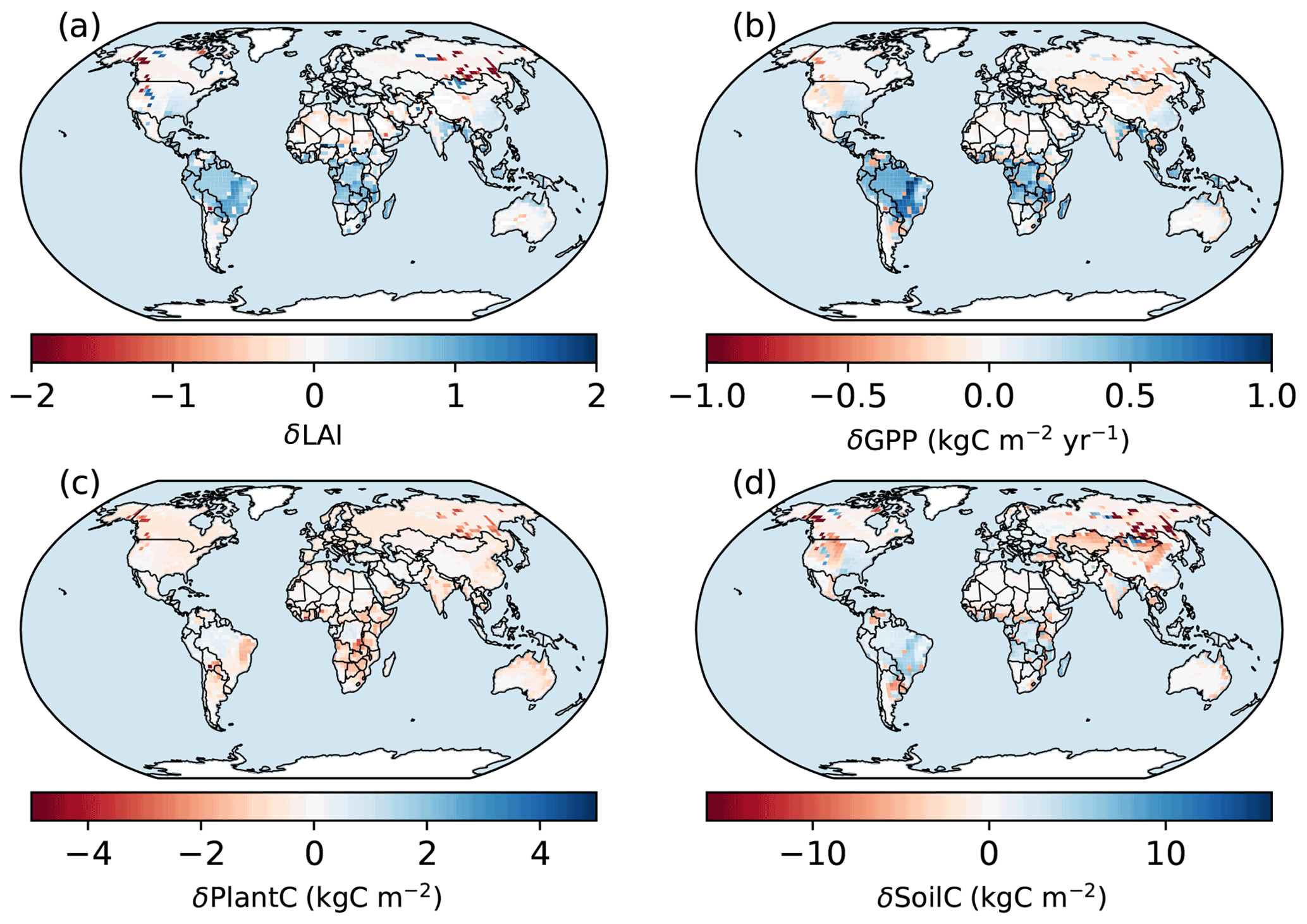
Figure 12 Spatial patterns of the differences between the simulations of the BiomeE. δ means the difference between the simulations of the full demography and the single-cohort models. LAI is the leaf area index, GPP is the gross primary production ($\mathrm{kg}\mathrm{C}{\mathrm{m}}^{-\mathrm{2}}{\mathrm{yr}}^{-\mathrm{1}}$), plant C is the vegetation biomass (kg C m⁻²), and soil C is the soil organic matter (kg C m⁻²).

Compared to the single-cohort model, the full demography model predicts higher LAI and GPP in warm and wet regions and lower LAI and GPP in cold and dry regions (Fig. 12a and b). The full demography model also predicts much lower biomass and soil carbon than the single-cohort model in cold and dry regions (Fig. 12c). The reduced biomass input from the full demography alone is causing the difference in SOM dynamics since the two models share the same SOM pools and turnover/decomposition processes. Demographic processes greatly reduce model stability because low reproduction and high mortality rates in dry and cold regions can greatly reduce the vegetation coverage. By contrast, the single-cohort model replaces these processes by the simplified turnover of plant carbon pools that allows plants to stay in extremely dry or cold conditions.

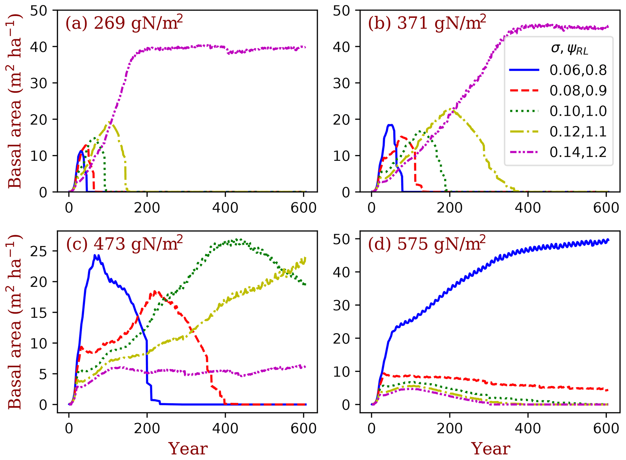
Figure 13 Simulated competitively dominant PFTs at different total ecosystem nitrogen. The simulations were set as nitrogen-closed (i.e., no input and output of nitrogen). The number in the title of each panel is the initial soil nitrogen. We used five PFTs that only differed in their LMA (σ) and target root/leaf area ratio (ϕ_RL) corresponding to each LMA in each simulation. Basal area (the sum of all the trees' trunk cross-sectional area) is used as the index of dominance.

4.4 Eco-evolutionary simulation and sensitivity test

The BiomeE model has the potential to predict competitively dominant PFTs in the continuum of plant traits through game–theoretic simulations, according to the principles of evolutionarily optimal competition. We illustrate this with a set of simulations conducted at a series of ecosystem nitrogen content (from 269 to 575 g N m⁻²), with five PFTs sampled from the continuums of LMA (σ; from 0.06 to 0.14) and the target root/leaf area ratio (ϕ_RL; from 0.8 to 1.2 corresponding to each LMA). The simulations were set as nitrogen-closed (i.e., no input or output of nitrogen). The differences in the ecosystem total nitrogen represent the environmental conditions that arise from soil and climate conditions. At the lowest ecosystem total nitrogen (Fig. 13a), the PFT with highest LMA (0.14 kg C m⁻² leaf) wins. As the ecosystem total nitrogen increases (Fig. 13b–d), the winner shifts from high to low LMA PFTs. This means that, in infertile soils or cold climates where biogeochemical cycles are slow (e.g., tundra and boreal forests), the eco-evolutionarily optimal PFTs should have high LMA leaves, and vice versa. This pattern is consistent with the predictions of a theoretical model in Weng et al. (2017). This simulation is also a case of the sensitivity test of vegetation dynamics at different environmental conditions. Vegetation can shift their compositions and dominant plant traits to maintain an eco-evolutionarily optimal state and thus amplify or attenuate the responses of ecosystem carbon cycle to climate changes.

5 Discussion

We developed a parsimonious terrestrial ecosystem model for ModelE to simulate vegetation dynamics and ecosystem biogeochemical cycles. This model includes a cohort-based representation of vegetation structure, a height-structured light competition scheme, demographic processes, and coupled carbon–nitrogen biogeochemical cycles. This model has four major modules that organize the hierarchical processes of ecosystems together into a cohesive modeling structure including (1) plant physiology (i.e., photosynthesis and respiration), (2) plant phenology and growth, (3) vegetation structural dynamics, and (4) soil biogeochemical cycles (Fig. 1). Each module is cohesive and has a minimum set of variables as the input from other modules.

5.1 Model formulation

In designing this model, we considered the simulation of competitively optimal strategy of plants in different climates based on fundamental ecological rules (Purves and Pacala, 2008; Falster and Westoby, 2003; Franklin et al., 2020). These strategies are mainly related to light competition, water conditions, nutrient use efficiency, and disturbances (e.g., fire) and are represented by the traits of wood density, height growth, leaf longevity, and photosynthesis pathways. PFTs are used in this model as an integrative unit representing combinations of plant traits for simulating (1) the spontaneous dynamics of carbon, water, and energy fluxes as the core functions of an ESM-based land model and (2) the transient vegetation structural and compositional dynamics and ecosystem biogeochemical cycles in response to climate variations.

We adopted a generic design of the PFTs by defining them as samples from the high-dimensional space defined by plant traits in their natural ranges. This approach substantially simplifies the parameterization of PFTs because it becomes the selection of strategies in different trait values (i.e., parameters). The numbers of PFTs are flexible, depending on what strategies the users wish to simulate (see the test simulations in Fig. 13). Thus, the PFTs are adaptive and variable in different environmental conditions, making it possible to reduce the number of PFTs while representing functional diversity and the optimal adaptation to climate conditions.

To represent the major variations in plant functional diversity, we chose the following four plant traits as the primary axes to define PFTs: wood density, LMA, height growth parameter, and leaf maximum carboxylation rate. Wood density is relatively conservative (Swenson and Enquist, 2007; Chave et al., 2009), mostly ranging from 200 to 500 kg C m⁻³, while herbaceous stem density ranges from 400 to 600 kg C m⁻³ (Niklas, 1995). However, herbaceous stems are usually hollow, making the ratio of total biomass to its volume low, and grasses shed their stems each growing season, resulting in faster stem turnover. It is a strategic difference from woody plants, which keep the woody tissues to build up their trunks and thus display their leaves on top of trunks for light competition (Dieckmann et al., 2007; Falster and Westoby, 2003). LMA is the key leaf trait that determines leaf life longevity and leaf types (i.e., evergreen vs. deciduous; Osnas et al., 2013) and represents the strategy for the competition in different soil nutrient levels (Tilman, 1988; Reich, 2014; Weng et al., 2017) and resistance to stresses of water and temperature (Oliveira et al., 2021).

The phenological type is simulated as an emergent property of plant physiological processes and strategies of dealing with seasonal air temperature and soil water variations. Three parameters – growing degree days, running mean daily temperature, and critical soil moisture – are used to define all possible phenological types. These three parameters are widely used in phenology modeling (e.g., Sitch et al., 2003; Prentice et al., 1992; Arora and Boer, 2005). However, phenology is not just a physiological response to the seasonality of climate conditions. Evergreen plants are distributed in periodically cold or dry climates. It is a competitively optimal strategy in infertile soil conditions (Aerts, 1995; Givnish, 2002; Coomes et al., 2005). The benefits and costs of keeping different leaves in cold or dry periods should be realistically simulated based on eco-evolutionary theories for phenology modeling (e.g., Levine et al., 2022; Weng et al., 2017).

As for soil organic matter decomposition, the Carnegie–Ames–Stanford approach (CASA) model, which has 13 pools with different transfer coefficients and turnover rates (Randerson et al., 1997; Potter et al., 1993, 2003), is currently used in ModelE. The soil biogeochemical cycle models developed thereafter have more sophisticated processes, especially those of microbial activities and carbon use efficiency (Manzoni et al., 2010; Wieder et al., 2014; Wang and Goll, 2021), and simplified carbon pools, mostly following the CENTURY model structure (Parton et al., 1987). We chose an intermediate complexity scheme that has only two SOM pools but a functional microbial pool for decomposing SOM (Manzoni et al., 2010; Weng et al., 2017) so that the dynamics of the SOM C:N ratio, carbon use efficiency, and nitrogen mineralization can be reasonably simulated while keeping the model structure parsimonious.

5.2 Model predictions and performance

We only evaluated the carbon cycle in the model simulations in this paper, though the nitrogen cycle is also simulated in tandem with the carbon cycle in the model. The major processes of this model, e.g., photosynthesis, respiration, phenology, growth, allocation, demography, soil biogeochemical cycles, are from well-developed models and have been shown able to capture observational patterns. Data assimilation approaches can be implemented when parameter tuning becomes essential (Luo et al., 2011; MacBean et al., 2016). So, we did not extensively tune model parameters to fit observations because the purpose of this paper is to describe the formulation of the model.

The simulations demonstrate that this model can capture the global patterns of LAI, GPP, tree height, biomass, and soil carbon (Fig. 7), even though the parameters are not extensively tuned. For example, global GPP patterns are consistent with those derived from SIF data (Figs. 7c, d and 8b), and simulated tree heights span the same ranges of those derived from data. The simulated LAI is segregated by PFTs (Fig. 8a), largely because of the different parameter values of the maximum crown LAI for each PFT. The simulated biomass and soil carbon are generally higher than those of observations, though simulated soil carbon is lower in some cold regions.

Several factors likely explain the apparent discrepancies between simulated and observed LAI, GPP, biomass, and soil carbon. First, the model uses a potential PFT distribution and does not account for land cover change and land use history. For example, carbon dense ecosystems (e.g., forests) have been extensively replaced by croplands and pastures. Second, while vegetation in the real world reflects a variety of successional stages and the effect of various disturbance events, our model analyses are based on equilibrium simulations without explicit disturbances, such as fire, deforestation, and regrowth. Third, the model assumes mineral nitrogen is saturated and can consistently meet demands for plant growth. We did not fix the land cover mismatches by compromising ecosystem physiological processes because we cannot put all these effects into current model structure (i.e., mortality) when many processes are missing.

LAI is an illustrative variable for understanding why compromises are necessary when integrating ecological and demographic processes into an ESM. As a critical prognostic variable in vegetation models, it links both plant physiology and biogeophysical interactions with climate systems (Richardson et al., 2012; Kelley et al., 2020; Park and Jeong, 2021). While LAI is usually simulated by a fixed allocation scheme, even if the allocation ratios are dynamic with vegetation productivity or environmental conditions (Montané et al., 2017; Xia et al., 2019), the prediction of LAI is often simplified as the balance between leaf growth and turnover.

In practice, modelers tend to tune the LAI to fit observations and obtain the required albedo and water fluxes, whatever the parameters of photosynthesis and respirations are. The uniform leaves within a crown would make the lower-layer leaves have a negative carbon gain if the LAI was tuned close to that observed in tropical and boreal evergreen forests (around 5–7). Therefore, the photosynthesis rate must be tuned to fit the canopy photosynthesis by keeping these carbon negative leaves. The crown with carbon negative leaves does not affect the ecosystem carbon dynamics in the single-cohort models because the whole canopy net carbon gain can be tuned to fit the observations. However, in demographic models, different-sized trees are explicitly represented and placed in specified crown layers. If the LAI is high, the vegetation community can create a dark understory where the seedlings cannot survive because of the negative carbon gain (Weng et al., 2015).

Since the leaf traits in the crown profile are functions of light, water, and nitrogen (Niinemets et al., 2015), a more complex crown development module is required to simulate branching and leaf development and deployment processes. Plants can optimize canopy leaf profile to maximize their fitness as a result of interactions among crown structure, light interception, and community-level competition (Anten, 2002; Hikosaka, 2005; Niinemets and Anten, 2009; Hikosaka and Anten, 2012). For balancing the model complexity and computing efficiency, we defined a low target LAI in this model to avoid carbon negative leaves.

The parameter V_cmax used in this model is also much lower than that measured in young leaves (Bonan et al., 2011). The mean photosynthetic capacity of the leaves in a crown affected the aging of leaves and their light environment (Niinemets, 2007; Kitajima et al., 2002; Hikosaka, 2005). The new leaves that are usually measured have much higher V_cmax than the mean of the canopy. If the leaves were not specifically chosen, then the mean of measured V_cmax is much lower than those used in models, as shown in Verryckt et al. (2022). This also indicates that V_cmax in current vegetation models is overestimated.

In this model, the formulation of allometry makes the whole tree's photosynthesis and respiration proportional to crown area and, thus, the growth rate of tree diameter independent of crown area. The allocation scheme between the growth of stems and functional tissues (i.e., leaves and fine roots) is the strategy of resources foraging for light and soil resources, including the height-structured competition for light. The vital rates drive vegetation structural changes and biogeochemical cycles (Purves et al., 2008). Our model allows the simulation of vegetation composition and structural dynamics based on the fundamental principles of ecology, and the transient changes in terrestrial ecosystems in response to climate change. This model therefore has the potential to predict competitively dominant strategies represented by plastic plant traits (e.g., the competitively dominant LMA in the simulations of Fig. 13), and the vegetation structure and compositions that can be eco-evolutionarily optimized.

5.3 Major uncertainties in BiomeE

Global vegetation models typically require simplifying assumptions to organize ecosystem processes at different scales into a cohesive model structure that balances the complexity of ecosystem processes and the limitations of our knowledge (Prentice et al., 1992, 2007; Harrison et al., 2021). In our model, many processes, including phenology and drought effects, are based on phenomenological equations representing the poorly understood links between processes needed by the model to simulate the entire system. In the following sections, we highlight these assumptions and evaluate their relative benefits and costs. Transparency in the description of a community model such as this one will help future developers understand model compromises and the processes that should be improved. The following phenomenological relationships represent the major sources of uncertainty in this model.

Water limitation of photosynthesis is calculated as a function of relative soil moisture, following the water stress function from Rodriguez-Iturbe et al. (1999):

$$\begin{array}{}\text{(16)}& {\mathit{\beta }}_{\mathrm{D}}=\text{Min}\left(\mathrm{1.0},\text{max}\left({\displaystyle \frac{s_{\mathrm{D}}-s_{\text{min}}}{s^{\ast }-s_{\text{min}}}},\mathrm{0.0}\right)\right).\end{array}$$

The parameters s^∗ and s_min are PFT specific, representing different responses of PFTs to soil water conditions, and S_D is the relative soil moisture ranging from 0 (soil water content at wilting point) to 1 (at field capacity). This formulation that scales soil moisture to a scalar between 0 to 1 is repeatedly used in both physiological responses of photosynthesis and phenology in ecosystem models as a simplistic treatment of the central role of water limitation on plant physiology (Powell et al., 2013; De Kauwe et al., 2015; Harper et al., 2021). This equation does not include the detailed processes of plant hydraulics and its adaptation to arid environments.

Multiple processes are involved to deal with water stress, such as regulating stomata conductance, shedding leaves, and producing more roots (Oliveira et al., 2021; Volaire, 2018). On top of these underlying processes, competition and evolutionary processes filter community-emergent properties (Franklin et al., 2020; van der Molen et al., 2011). For example, trees in different climate regions have similar hydraulic safety margins (Choat et al., 2012), partly due to the intense competition for light (height growth) and water (root allocation) that require the optimal use of available resources at any climate conditions (Gleason et al., 2017; Liu et al., 2019). However, in this model, the drought responses are only delineated by Eq. (16). The parameter choices for s^∗ and s_min likely explain the amplified water stresses and low productivity in arid regions within our model.

Phenology represents the seasonal rhythms of plant physiological activities as adapted to periodic changes in temperature, precipitation, and light availability (Abramoff and Finzi, 2015; Caldararu et al., 2014; Chuine, 2010). DGVMs normally simulate leaf onset and senescence based on temperature conditions for cold deciduous plants and soil water conditions for drought deciduous plants (Arora and Boer, 2005; Caldararu et al., 2014). Phenology modeling is still highly empirical, although new models and approaches for cold deciduous and drought deciduous strategies have been proposed recently (e.g., Caldararu et al., 2014; Dahlin et al., 2015; Manzoni et al., 2015; Chen et al., 2016). We used a simple formulation of temperature and drought responses (Eqs. 1 and 3). These relationships are phenomenological. Future model development should incorporate eco-evolutionary mechanisms that are selected in the evolution history.

Mortality is an integrative process of accumulative physiological stresses, structural damages, and disturbances in a tree's lifetime. The direct causes can be starvation, structural failure, hydraulic failure, etc. (McDowell, 2011; Aakala et al., 2012; Aleixo et al., 2019). We only consider the background mortality and define its rate as a function of tree diameter and light environment (Eq. 10). Hydraulic-failure-induced mortality is required for realistically modeling plant responses to climate changes.

We used these general phenomenological equations primarily because of our knowledge gaps in ecosystem ecology. We are using the key variables that characterize ecosystem properties to define the basic model structure but have to use less-than-solid information to link them together by phenomenological relationships, as all the models do. In addition, our interest is to keep this model as simple as possible to improve the interpretability and transparency and to reduce the computational burden when it is integrated into the ModelE. In these places where the tradeoff between model complexity and process accuracy is necessary, we highlight the underlying assumptions clearly, rather than implementing temporary fixes that lack solid empirical evidence.

5.4 Insights from comparison with MsTMIP models

Most MsTMIP participant models used in this study have been analyzed by a model traceability method developed by Xia et al. (2013), which hierarchically decomposes model behavior into some fundamental processes of ecosystem carbon dynamics, such as GPP, CUE, allocation coefficients, carbon residence time, carbon storage capacity, and environmental response functions (Xia et al., 2013; Cui et al., 2019; Zhou et al., 2021). This method is based on the assumptions of the linear system and the ecosystem-emergent behavior per se (Eriksson, 1971; Emanuel and Killough, 1984; Luo et al., 2012; Sierra et al., 2018), making it is consistent with the concepts that are used as the basis of ecosystem carbon cycle models. The analyses of model traceability found that, for the carbon cycle dynamics, the major uncertainty is from the modeling of the turnover rates (reciprocals of residence time) of vegetation and soil carbon pools (Chen et al., 2015; Jiang et al., 2017). From CMIP5 to CMIP6, the modeling of NPP has been greatly improved, while the ecosystem carbon residence time remains highly biased (Wei et al., 2022).

According to the traceability analysis approach (Xia et al., 2013), BiomeE also has a high uncertainty in the modeling of residence times of vegetation and soil carbon pools because the mortality is picked up from the global forest data and the SOM decomposition processes are highly simplified. These issues have been discussed in Sect. 5.3. These concepts (e.g., residence time and allocation coefficients) describe model-emergent properties resulting from the underlying biological and ecological processes (i.e., micro-dynamics vs. macro-states). Fitting the emergent properties directly to improve model behavior is natural and convenient because many vegetation models are using these emergent properties (e.g., CUE, residence time, and allocation coefficients) to describe ecosystem processes in their formulations as a tradition of ecosystem modeling.

There are some common and long-lasting issues in terrestrial ecosystem modeling, such as responses to warming, responses to atmospheric CO₂, drought stress effects, and vegetation compositional changes (Luo, 2007; Franklin et al., 2020; Harrison et al., 2021). These issues represent our knowledge gaps in ecosystem ecology. For modeling vegetation dynamics eco-evolutionarily, we need to use the fundamental ecological processes and unbreakable physical rules to simulate the emergent processes (e.g., Scheiter et al., 2013; Weng et al., 2019). With the design of vegetation modeling in the BiomeE, such as the explicit demographic processes, individual-based competition for different resources, and flexible trait combinations of PFTs, this model is able to predict some key emergent dynamics of ecosystems based on the underlying biological and evolutionary mechanisms (as shown in Fig. 13). Data from field experiments (Ainsworth and Long, 2004; Crowther et al., 2016), observatory networks (e.g., Fluxnet, Baldocchi et al., 2001; Friend et al., 2007), and remote sensing (Duncanson et al., 2020), can provide direct information for modeling the underlying ecological processes and for validating predicted emergent properties.

5.5 Model stability and complexity

Ecosystem demographic processes (e.g., reproduction and mortality) are a source of high sensitivity and uncertainty in BiomeE. In some environmental conditions, especially in dry or cold regions, the predefined parameters can lead to high mortality or failure of reproduction, making the ecosystems highly instable. To understand these issues, we used the single-cohort version of the model to aid in the diagnosis of issues in the full demographic version of the model. The major issue we identified is that the model formulation is based on functional processes in highly productive regions, whereas the model is applied globally and across much more diverse environmental conditions (e.g., arid environments). The variables and parameters that work well in highly productive regions (e.g., initial seedling sizes, default leaf growth, and minimum allocation ratios) are often unsuitable in regions with high environmental stresses. Although plants have evolved special features to deal with extreme conditions (Lloret et al., 2012; Reyer et al., 2013; Singh et al., 2020), these features have not yet been well represented in ecosystem models.

There is a tendency in current DGVMs to use plant physiological trait changes as a surrogate of community compositional shifts. This approach is usually characterized as parameter dynamics or response functions (Fisher and Koven, 2020; Luo and Schuur, 2020) for reducing model processes and complexity. Adding new processes to work around existing problems, instead of redesigning the fundamental model processes, is common in model development. It is helpful for tracking model development, undoing wrong additions, and improving model performance. However, workarounds often increase model complexity without concomitant improvements in model predictions.

Generally, a model's traceability can be improved by transparent assumptions, a well-defined model structure, and testable output (Famiglietti et al., 2021; Forster, 2017; Hourdin et al., 2017). Data assimilation approaches improve model parameterization more efficiently and effectively than manually tuning individual parameters (Wang et al., 2009; Williams et al., 2009; MacBean et al., 2016) and allow for more detailed uncertainty analysis (Luo et al., 2009; Weng et al., 2011; Weng and Luo, 2011; Xu et al., 2006; Dietze, 2014). It is important to only include necessary assumptions in a model and to include them in a way that does not compromise other processes or parameters. Additionally, many specifications of model formulation are based on the questions of specific research. We should not expect to develop an all-encompassing model that fits all application scenarios. On the contrary, maintaining model flexibility and transparency is critical for using this model as a tool to explore specific science questions. In BiomeE, we have opted for what we consider the most parsimonious and, at the same time, theoretically sound formulations of ecosystem processes to allow for computational efficiency in capturing vegetation dynamics and ecological principles in the context of an ESM.

5.6 Legacy limitations of ModelE coding and development conventions

The legacy of model structure and the history of model development can greatly affect the functions and the selection of model formulations (Alexander and Easterbrook, 2015). ModelE was developed as a general circulation model, and vegetation in the model to date has been represented with a set of static biophysics parameterizations to regulate exchanges of energy and moisture between the land surface and the atmosphere (Hansen et al., 2007; Schmidt et al., 2014; Kelley et al., 2020). To advance the functionality of the vegetation and the land surface model within ModelE, increases in complexity must therefore be balanced with the computational demands of the fully coupled model.

In ModelE, the land model, TerraE, is used to calculate land surface (including vegetation) water and energy fluxes and soil water dynamics based on the characteristics of vegetation derived from the vegetation model (canopy conductance, wetness, etc.) at the grid scale. It does not calculate each cohort's transpiration and water uptake. In BiomeE, the water limitation of stomatal conductance is calculated as a function of soil water stress index and root vertical distribution, instead of the direct plant root water supply (plant hydraulics). This setting works well for the big-leaf model (one canopy at one grid). However, when multiple cohorts of plants are represented, as we do in BiomeE, it is unable to represent water competition and differentiate the contribution of each single cohort's contribution to the total transpiration. A structural change will be required to solve this problem by calculating transpiration from the bottom-up (i.e., from cohort up to grid cell).

6 Conclusions

We developed a demographic vegetation model to improve the representation of terrestrial vegetation dynamics and ecosystem biogeochemical cycles in the NASA GISS Earth system model, ModelE. This model includes the processes of plant growth, mortality, reproduction, vegetation structural dynamics, and soil carbon and nitrogen cycling. To scale this model globally, we added a new set of plant functional types to represent global vegetation functional diversity and introduced new phenology algorithms to deal with the seasonality of temperature and soil water availability. Competition for light and soil resources is individual based, which makes the modeling of eco-evolutionary optimality possible. This model predicts the dynamics of vegetation and soil biogeochemistry, including leaf area index, vegetation structure (e.g., height, tree density, size distribution, crown organization), and ecosystem carbon and nitrogen storage and fluxes. This model will enable ModelE to simulate long-term biogeophysical and biogeochemical feedbacks between the climate system and land ecosystems at decadal to centurial temporal scales. It will also allow for the prediction of transient vegetation dynamics and eco-evolutionary community assemblage in response to future climate changes.