Impact of physical parameterizations on wind simulation with WRF V3.9.1.1 under stable conditions at planetary boundary layer gray-zone resolution: a case study over the coastal regions of North China

Reliable simulation of wind fields under stable weather conditions is vital for preventing air pollution. In this study, we investigate how different physical parameterizations impact simulated near-surface wind at 10 m height over the coastal regions of North China using the Weather Research and Forecasting (WRF) model with a horizontal grid spacing of 0.5 km. We performed 640 simulations using combinations of 10 planetary boundary layer (PBL), 16 microphysics (MP), and four shortwave–longwave radiation (SW–LW) schemes. Model performance is evaluated using measurements from 105 weather station observations. The results show that the WRF model can reproduce the temporal variation of wind speed in a reasonable way. The simulated wind speed is most sensitive to the PBL schemes, followed by SW–LW schemes and MP schemes. Among all PBL schemes, the MYJ scheme shows the best temporal correlation with the observed wind speed, while the Yonsei University (YSU) scheme has the lowest model bias. Dudhia–RRTM and MYDM7 show the best model performances out of all SW–LW and MP schemes, respectively, and the interactions among schemes also have large influences on wind simulation. Further investigation indicates that model sensitivity is also impacted by ocean proximity and elevation. For example, for coastal stations, MYNN shows the best correlation with observations among all PBL schemes, while Goddard shows the smallest bias of SW–LW schemes; these results are different from those of inland stations. In general, according to the bias metrics, WRF simulates wind speed less accurately for inland stations compared to coastal stations, and the model performance tends to degrade with increasing elevation. The WRF model shows worse performance in simulating wind direction under stable conditions over the study area, with lower correlation scores compared to wind speed. Our results indicate the role parameterizations play in wind simulation under stable weather conditions and provide a valuable reference for further research in the study area and nearby regions.

1 Introduction

Megacities that experience rapid urbanization and economic development also commonly suffer from a simultaneous decline in air quality (Ulpiani, 2021). For example, many haze events have been reported in the Beijing, Tianjin, and Hebei regions of North China over the past few decades. Haze-related weather and associated high concentrations of fine particulate matter have negative impacts on public health and the environment (Wang and Mauzerall, 2006). These events can significantly disrupt economic growth, as demonstrated by the severe haze events that occurred over North China in January 2013 (Zhang et al., 2014, 2015; Cai et al., 2017). The haze events are most frequent in boreal winter and are closely related to local weather conditions with low wind speeds (Li et al., 2015; Wang et al., 2021). Projections of future climate change suggest that global temperatures and weather conditions conducive to severe haze will increase, affecting North China (Cai et al., 2017). However, numerical models often show a large bias in wind prediction over China (X. Gao et al., 2016; Zhao et al., 2016; Pan et al., 2021), and thus it is crucial to improve wind prediction under stable weather conditions in order to minimize associated economic losses and environmental impacts.

In recent years, numerical models have been used extensively to study and forecast the weather and climate over China, as they have high spatial and temporal resolutions and employ sophisticated physical parameterization schemes that can reproduce atmospheric and land surface processes (Wang et al., 2011; Zhou et al., 2019; Kong et al., 2022). However, studies mostly focus on temperature or precipitation, and only a few have attempted to simulate winds over China (Li et al., 2019; Xia et al., 2019; Pan et al., 2021). Meanwhile, numerical models inherently involve many sources of uncertainty, as they cannot resolve all processes in the real world; instead, parameterizations are needed to represent the effect of key physical processes, such as radiative transfer, turbulent mixing, and moist convection that occur at the sub-grid scale. Different physical parameterization schemes depict natural phenomena to different degrees of accuracy, and choosing appropriate combinations is important, as it can strongly influence model results (Yu et al., 2011; Gómez-Navarro et al., 2015; Stegehuis et al., 2015; X. Gao et al., 2016; Yang et al., 2017; Taraphdar et al., 2021).

The impact of the planetary boundary layer (PBL) scheme on wind simulation has been studied for many years, as the PBL scheme plays a critical role in modulating mass, energy, and moisture fluxes between the land and atmosphere, which in turn influences the simulation of low-level temperatures, cloud formation, and wind fields (Jiménez and Dudhia, 2012; Gómez-Navarro et al., 2015; Gonçalves-Ageitos et al., 2015; Falasca et al., 2021; Gholami et al., 2021). Many studies indicate an overestimation of wind speed in WRF simulations with different PBL schemes (Jiménez and Dudhia, 2012; Carvalho et al., 2014a, b; Pan et al., 2021; Gholami et al., 2021; Dzebre and Adaramola, 2020). For example, Gómez-Navarro et al. (2015) investigate the sensitivity of the WRF model to the PBL scheme by simulating wind storms over complex terrain at a horizontal grid spacing of 2 km. In that study, the WRF model is configured with the Mellor–Yamada–Janjic (MYJ) scheme and overestimates wind speed by up to 100 %; however, the bias is significantly reduced when the non-local scheme developed at Yonsei University (YSU) is used instead. The YSU scheme also shows good model skill in simulating winds over the Iberian Peninsula, Persian Gulf, Tyrrhenian coast, and western Argentina (Jiménez and Dudhia, 2012; Puliafito et al., 2015; Falasca et al., 2021; Gholami et al., 2021). Other studies suggest that MYNN and ACM2 are more appropriate for wind simulations (Carvalho et al., 2014b; Chang et al., 2015; Prieto-Herráez et al., 2021; Rybchuk et al., 2021).

The performance of wind simulation is also influenced by the choice of cloud microphysics (MP) parameterizations. Cloud microphysical processes, such as moisture evaporation and condensation, can change thermodynamic and dynamic interactions in the atmosphere (Rajeevan et al., 2010; Cheng et al., 2013; Santos-Alamillos et al., 2013; Li et al., 2020) and then affect the vertical distribution of heat and wind fields close to the surface.

Another factor influencing wind simulation is the choice of radiation parameterizations, which include shortwave radiation and longwave radiation (SW–LW) schemes. Differences in surface radiation intensities can generate thermal contrasts in regions with complex topography, which in turn affect local and low-level wind distribution patterns (Santos-Alamillos et al., 2013).

The combinations of physical parameterizations are also vital to wind simulation, as the processes of atmosphere–land interactions, radiation transport, and moist convection interact and may amplify the uncertainties in wind prediction. The impact of parameterization scheme combinations on WRF performance has been investigated in previous studies (Santos-Alamillos et al., 2013; Fernández-González et al., 2018), and Fernández-González et al. (2018) report that there is no single combination of schemes that performs best during all weather conditions. Most of the aforementioned studies considered a small number of parameterization schemes. To our knowledge, the sensitivity of parameterizations to wind simulation has not been explored in a systematic way in China. In this study, we systematically evaluate the performance of a large number of parameterization combinations, including PBL, MP, and SW–LW schemes. The investigation is conducted using the WRF model at a grid spacing of 0.5 km, which belongs to the PBL “gray zone” resolution that is too fine to utilize mesoscale turbulence parameterizations and too coarse for large-eddy-simulation (LES) schemes to resolve turbulent eddies (Shin and Hong, 2015; Honnert et al., 2016). Our main objective is to identify a set of configurations of the WRF model that can best reproduce wind fields under stable weather conditions over North China, which experienced many haze events during the past few years. This study addresses the following research themes: (1) quantify the sensitivity of wind simulation to different parameterizations under stable weather conditions and (2) refine optimized configurations with the best performance in reproducing winds under stable weather conditions over North China. These results would provide a valuable evaluation of WRF performance using a large number of simulations with different physical parameterizations and be helpful in the wind and air quality forecasts in the study area and other coastal regions of China under stable weather conditions.

2 Data and methods

2.1 The stable weather event in 2019

The study area is located in the central section of the “Bohai Economic Rim”, which is bordered to the southeast by the Bohai Sea and to the northwest by the Yan Mountains (Fig. 1a). This region traditionally hosts heavy industry and manufacturing businesses and is a significant region of economic growth and development in North China (Song et al., 2020; Zhao et al., 2020). Air quality in this area has declined over the past decades, and the frequency of winter haze events has increased due to increased pollutant emissions and favorable stable weather conditions with lower wind speed (M. Gao et al., 2016; Cai et al., 2017). For instance, during the heavy fog and haze event over eastern China in January 2013, an anomalous southerly wind in the lower troposphere caused by the weak East Asian winter monsoon weakened the synoptic forcing and extent of vertical mixing in the atmosphere, thus increasing the stability of air in the boundary layer and the local concentration of hazes (Zhang et al., 2014).

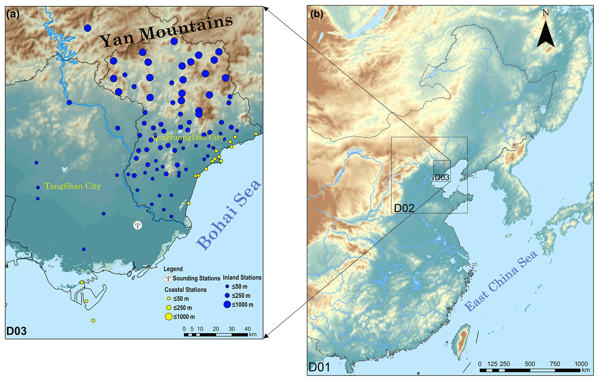
Figure 1 Map showing the (a) study area and (b) WRF nested domains (D01–D03). Solid yellow and blue circles in panel (a) represent coastal (16 stations in total) and inland stations (89 stations in total), the sizes of the circles represent the station elevations, and the white circle represents the sounding station.

During 11–15 January 2019, a severe haze event occurred in the study area, the peak PM_2.5 and PM₁₀ concentrations exceeded 279 and 357 µg m⁻³ in Tangshan city, and 282 and 358 µg m⁻³ in Qinhuangdao city, respectively, the locations of the two cities can be found in Fig. 1. Figure 2 depicts the distribution of geopotential height at 500 hPa, surface winds at 10 m and total cloud fraction from the ERA5 dataset (Hersbach et al., 2020) during the study period. A weak high-pressure system persisted from 11 to 14 January 2019 over the study area, with the geopotential height at 500 hPa of about 5400 gpm, at the surface level (10 m), weak southwest winds occurred at the south side of the study area on 11, 12 and 14 January 2019. The surface wind speeds over the study area were weaker than 5 m s⁻¹ during the first 4 d of the study period , and then the geopotential height decreased and strong northwesterly winds occurred over the study area on 15 January 2019. Although there were slight differences between ERA5 and satellite products (e.g., CLARA, Karlsson et al., 2021), both datasets indicated higher cloud fraction on 11 and 14 January 2019, while for the rest of the time, the cloud fraction was low. This stable weather event is used to investigate the impact of physical parameterizations of the WRF model.

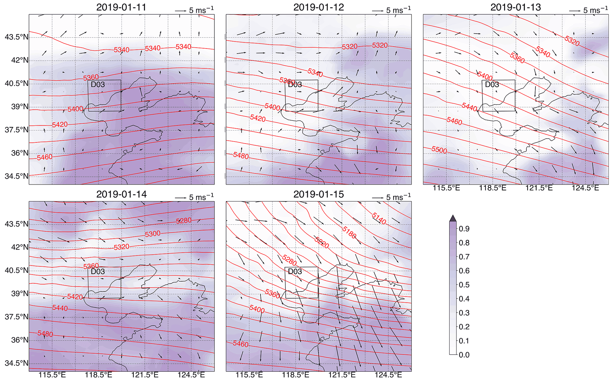
Figure 2 The daily averaged geopotential height (contour lines, units: gpm) at 500 hPa, total cloud fraction (shading), and surface winds at 10 m (vectors, units: m s⁻¹) from ERA5 during 11–15 January 2019; the box indicates the D03 domain in Fig. 1.

2.2 Model configurations

The WRF model (version 3.9.1.1) with the advanced research WRF (ARW) core is used in this study, which is a non-hydrostatic atmospheric model with terrain-following vertical coordinates (Skamarock et al., 2008). The simulations contain three one-way nested domains with grid spacings of 8, 2, and 0.5 km for D01, D02, and D03, respectively (Fig. 1b). The computational domains are based on Lambert conformal conic projection centered at 38.5^∘ N and 120^∘ E, with 360×480, 381×381, and 341×421 grid points for D01, D02, and D03, respectively. The evaluations are based on the innermost domain, which covers the coastal and surrounding regions of North China (Fig. 1a). The simulation domain has 65 vertical levels, and the eta values for the first 10 levels are 0.996, 0.988, 0.978, 0.966, 0.956, 0.946, 0.933, 0.923, 0.912, and 0.901: this ensures that sufficient model levels exist within the PBL at any time.

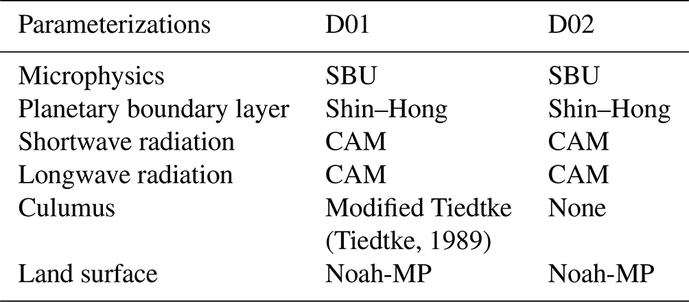
The ERA5 reanalysis dataset, which has a horizontal resolution of 0.25^∘ and 38 vertical levels, is used to provide the initial and boundary conditions for WRF simulations. The WRF model is initialized at 00:00 UTC (08:00 in local time) on 9 January 2019, with the first 40 h treated as the spin-up period. Firstly, the default physical parameterization schemes (Table 1) are applied in the WRF simulation for the outer two domains (D01 and D02), and then the output of D02 is used to drive inner-domain simulations with different combinations of PBL, MP, and SW–LW schemes (see Sect. 2.3). This approach helps to isolate the impacts of parameterization within the inner domain from changes in boundary forcing (Yang et al., 2017). All simulations apply the Noah land surface model with multi-parameterization options (Noah-MP, Yang et al., 2011; Niu et al., 2011) as the land surface parameterization scheme. The lateral boundary conditions and sea surface temperature are updated every 3 h using the ERA5 reanalysis data, and the frequency of wind retrieved from WRF output is hourly, which matches the frequency of observations in the study area.

Table 1 List of default parameterization schemes for the simulation of outer domains (D01 and D02).

2.3 Experimental design

The WRF model contains different parameterization schemes that represent different physical processes. Further, every scheme in the model has many parameters, such that a model can range from being simple and efficient to be sophisticated and computationally costly. In this study, a systematic evaluation of parameterizations is achieved by considering 10 PBL, 16 MP, and 4 LW-SW schemes, which produce 640 (i.e., $\mathrm{10}\times \mathrm{16}\times \mathrm{4}$) combinations in total.

The parameterization schemes investigated in this study are listed in Table 2. As the horizontal grid spacing of 0.5 km is within the PBL gray zone resolution, both PBL and LES assumptions are imperfect: we test both the PBL and LES schemes in this study. For the LES configuration, the 1.5-order turbulence kinetic energy closure model is used to parameterize motion at the sub-grid scale (Deardorff, 1985). For the YSU scheme, topographic correction for surface winds is included to represent extra drag from sub-grid topography and enhanced flow at hilltops (Jiménez and Dudhia, 2012). The option for top-down mixing driven by radiative cooling is also turned on during the integration. For the rest of the PBL schemes, the default configurations are chosen. The atmospheric surface layer (SL) is the lowest part of the atmospheric boundary layer, of which the parameterizations are used to quantify surface heat and moisture fluxes in the land surface model and surface stress in the PBL schemes. In the current generation of WRF, the SL schemes are tied to the PBL schemes. In this study, the ETA, QNSE, MYNN, Pleim-Xiu, and TEMF SL schemes are chosen for the PBL schemes of MYJ, QNSE, MYNN, ACM2, and TEMF, respectively. The revised MM5 scheme (Jimenez et al., 2012) is used for the remaining PBL schemes.

Table 2 List of microphysics (MP), planetary boundary layer (PBL), and shortwave–longwave radiation (SW–LW) schemes investigated in the 640 simulations; schemes that share rows are not specifically assigned to each other (except for SW–LW).

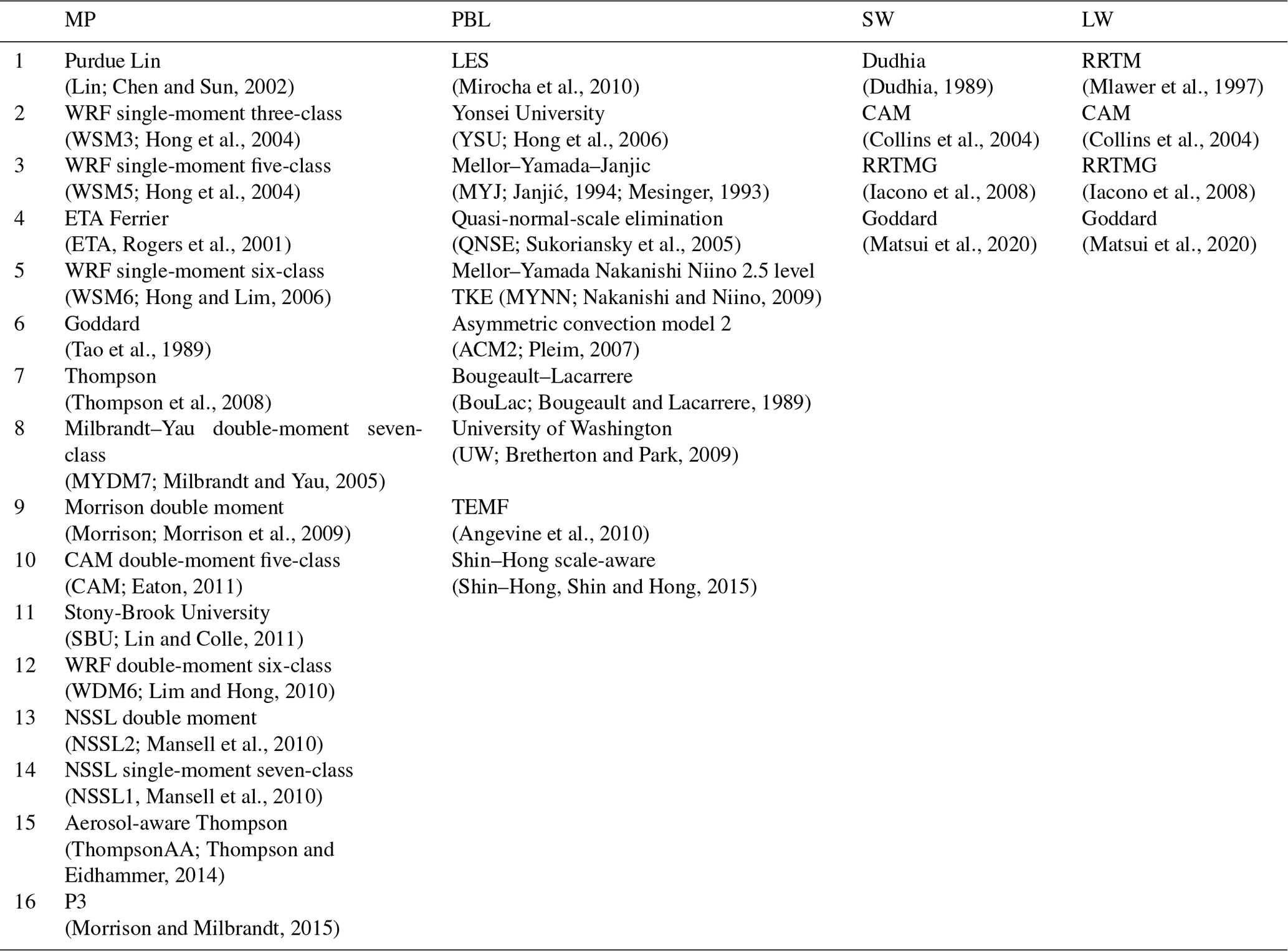
Sixteen MP schemes are applied in this study (Table 2), Lin, WSM3, WSM5, ETA, WSM6, Goddard, SBU, and NSSL1 schemes are the single-moment bulk microphysical scheme, which predicts only the mixing ratios of hydrometeors (i.e., cloud ice, snow, graupel, rain, and cloud water) by assuming particle size distributions. The other eight schemes (Thompson, MYDM7, Morrison, CMA, WDM6, NSSL2, ThompsonAA and P3) use a double-moment approach, predicting not only mixing ratios of hydrometeors, but also number concentrations. Among them, two types of hydrometeors are included in WSM3 (cloud water and rain), three types of hydrometeors are included in ETA (cloud water, rain, and snow) and P3 (cloud water, rain, and ice), four types of hydrometeors are included in WSM5 and SBU (cloud water, rain, ice, and snow), five types of hydrometeors are included in Lin, WSM6, Goddard, Thompson, Morrison, CAM, WDM6 and ThompsonAA (cloud water, rain, ice, snow, and graupel), six types of hydrometeors are included in MYDM7, NSSL1, and NSSL2 (cloud water, rain, ice, snow, graupel, and hail).

Four SW–LW combinations are applied in this study (Table 2), Dudhia is a simple and efficient shortwave radiation scheme for clouds and clear-sky absorption and scattering; RRTM provides efficient look-up tables for longwave radiation; CAM SW–LW schemes are derived from the CAM3 model used in CCSM3 and allow modeling of aerosols and trace gases. RRTMG is a scheme that utilizes Monte Carlo independent column approximation (MCICA) method of random cloud overlap.

2.4 Observational data and evaluation metrics

Observations from weather stations across the study region are used to evaluate the performance of the model. These stations are operated by the China Meteorology Administration (CMA) and report wind speed and direction at an altitude of 10 m. In this study, we use 2 min averaged wind speed at hourly frequency. All data are screened before analysis in order to remove stations with data showing spurious jumps (e.g., wind speed jumps to 0 m s⁻¹ due to the frozen sensor). After this filtering, 105 out of 132 weather stations (Fig. 1a) remained, including 89 inland stations and 16 coastal stations. The results of WRF are directly compared with observations at each weather station, which is achieved by using the model result that is geographically closest to the weather station under consideration. Although some errors are introduced when performing these comparisons, they are systematic and shared by all simulations and therefore have minor effects on the evaluation of model performances.

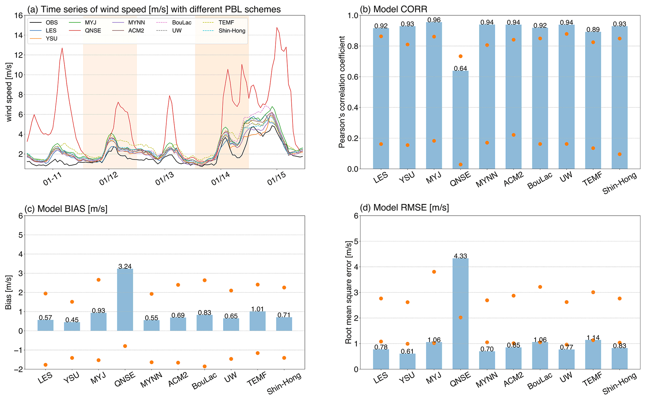
Figure 3 (a) Time series of observed and simulated wind speeds (m s⁻¹) and the corresponding statistics of (b) CORR, (c), BIAS, and (d) RMSE for the PBL schemes. In panel (a), the frequency of wind speed is hourly, and the tick marks on the x axis indicate 12:00 LT of that day, for each PBL scheme, and the average is calculated over the 105 stations and then over all the simulations with that scheme. The dots in panels (b)–(d) represent the range across the stations, for each station, and the metrics are calculated by averaging all the simulations with the specific PBL scheme.

Several metrics are employed for evaluating the performance of each model configuration, including the Pearson correlation coefficient (CORR), BIAS, root mean square error (RMSE), and Taylor skill score (T). CORR is a measure of the strength and direction of the linear relationship between simulation and observation, BIAS is a measure of the mean difference between simulation and observation, and RMSE is the square root of the average of the set of squared differences between simulation and observation, and thus each of these scores gives a partial view of the model performance.

They are defined as follows:

$$\begin{array}{c}{\displaystyle }\text{CORR}={\displaystyle \frac{{\sum }_{i=\mathrm{1}}^N(M_i-\stackrel{\mathrm{‾}}{M})(O_i-\stackrel{\mathrm{‾}}{O})}{\sqrt{{\sum }_{i=\mathrm{1}}^N(M_i-\stackrel{\mathrm{‾}}{M}{)}^{\mathrm{2}}\cdot {\sum }_{i=\mathrm{1}}^N(O_i-\stackrel{\mathrm{‾}}{O}{)}^{\mathrm{2}}}}},\\ {\displaystyle }\text{BIAS}={\displaystyle \frac{\mathrm{1}}{N}}\sum _{i=\mathrm{1}}^N\left(M_i-O_i\right)\\ {\displaystyle }\text{RMSE}=\sqrt{{\displaystyle \frac{\mathrm{1}}{N}}{\sum }_{i=\mathrm{1}}^N(M_i-O_i{)}^{\mathrm{2}}},\\ {\displaystyle }T={\displaystyle \frac{\mathrm{2}(\mathrm{1}+\text{CORR})}{{\left(\text{SD}+\frac{\mathrm{1}}{\text{SD}}\right)}^{\mathrm{2}}}}.\end{array}$$

Here, M is the value of the model output, O is the value of the observation, N is the number of observations, and SD is the ratio of simulated-to-observed standard deviation. A higher Taylor skill score indicates a more accurate simulation (Gan et al., 2019), while higher CORR, lower BIAS, and RMSE scores indicate better model simulations.

The difference in wind direction was calculated as follows.

$$\mathrm{\Delta }=\left\{\begin{array}{ll}M-O,& \text{when }|M-O|\le \mathrm{180}{}^{\circ }\\ (M-O)\left(\mathrm{1}-{\displaystyle \frac{\mathrm{360}}{|M-O|}}\right),& \text{when }|M-O|>\mathrm{180}{}^{\circ }\end{array}\right.$$

The correlation between simulated and measured angles is determined by a circular correlation coefficient, and the mean of the angular is calculated using the vector notation approach. The circular correlation coefficient is calculated as follows.

$$\text{CORR}={\displaystyle \frac{{\sum }_{i=\mathrm{1}}^N\sin \left({\mathit{\alpha }}_i-\stackrel{\mathrm{‾}}{\mathit{\alpha }}\right)\sin ({\mathit{\beta }}_i-\stackrel{\mathrm{‾}}{\mathit{\beta }})}{\sqrt{{\sum }_{i=\mathrm{1}}^N{\sin }^{\mathrm{2}}\left({\mathit{\alpha }}_i-\stackrel{\mathrm{‾}}{\mathit{\alpha }}\right){\sin }^{\mathrm{2}}({\mathit{\beta }}_i-\stackrel{\mathrm{‾}}{\mathit{\beta }})}}}$$

Here, α and β are simulated and observed wind direction angles, respectively.

3 Results

3.1 Impacts of physical parameterizations

3.1.1 PBL

Figure 3a shows the time series of observed wind speed in local time. Model wind speeds are shown for different PBL schemes averaged over all other parameterization types. The WRF model generally reproduces the temporal variation of observed wind speed in the study area with exaggeration; in particular, the shift from low to high wind speed on 14 January 2019 is reproduced by all schemes except for QNSE, with which the wind speed change is considerably larger than with all other schemes during the simulation period. Almost all the PBL schemes overestimate wind speed by 1 m s⁻¹; however, for the QNSE scheme, the largest overestimation exceeds 10 m s⁻¹ during the daytime on 11 and 15 January 2019. The difference between simulation and observation is lower during 11–13 January 2019 using the LES scheme, while YSU is more similar to the measurements during 14–15 January 2019. In addition, the spread within the PBL schemes is larger on 15 January 2019, partly due to the high wind speed (>4 m s⁻¹) or the general error growth in the model.

The statistics of CORR, BIAS, and RMSE are illustrated in Fig. 3b–d. MYJ shows the best CORR score of 0.96; MYNN, ACM2, and UW are the next best according to this verification score. YSU is the best scheme in terms of BIAS and RMSE, with the values of 0.45 and 0.61 m s⁻¹ followed by MYNN (0.55 and 0.70 m s⁻¹). The ranges of statistic scores across the 105 stations are also illustrated in Fig. 3, for the schemes except for QNSE, and the range of CORR is 0.18–0.88, the range of BIAS is −2.10–2.91 m s⁻¹, and the range of RMSE is 0.79–3.85 m s⁻¹. Further comparison indicates that the CORR scores for individual stations are lower than the ensemble means, and the BIAS and RMSE are larger than the ensemble means. For the QNSE scheme, the maximum BIAS and RMSE scores for individual stations exceed 10 and 16 m s⁻¹, indicating that it has problems in reproducing wind speed under stable conditions over the study area.

Figure 4 shows the wind roses during 11–15 January 2019 from observations and simulations with different PBL schemes as well as the statistic scores. Observations indicate that, during the study period, wind is mostly from a southwesterly-to-northwesterly direction (225–330^∘), while simulations with different PBL schemes produce primarily southwesterly wind (200–270^∘), indicating an anticlockwise bias of wind direction over the study area under stable conditions. Further comparison indicates that all PBL schemes strongly overestimate the speed of northerly wind compared to the observations, which may be the main cause of positive bias in wind speed (Fig. 3). The CORR scores of wind direction (0.42–0.59) are notably lower than those of wind speed, indicating the degraded performance of WRF in wind direction simulation. LES shows the best CORR score of 0.59, while TEMF shows the best BIAS and RMSE scores of −11.33 and 56.19^∘. Considering the large model bias in wind speed, simulations with the QNSE scheme (64 in total) are omitted from further investigation in order that these anomalous data do not affect our overall analysis.

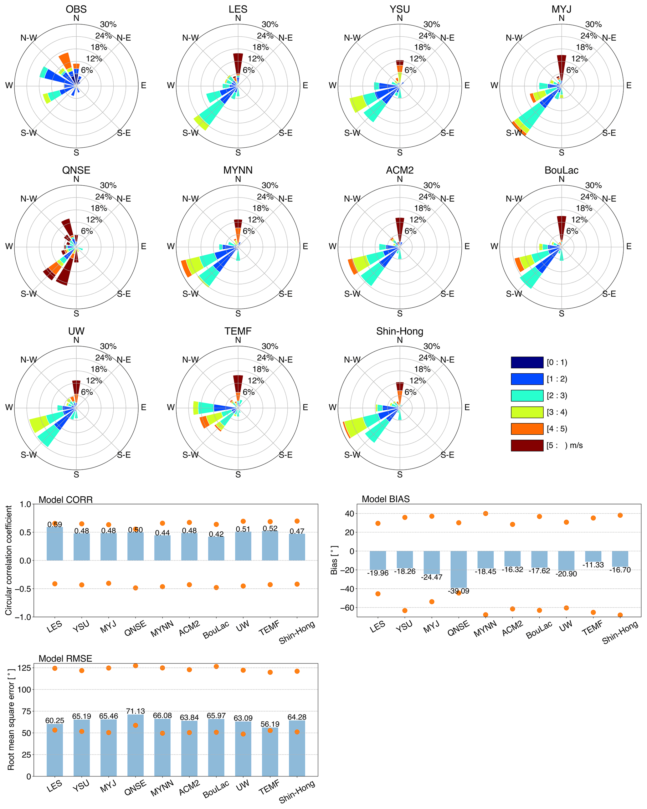
Figure 4 The wind rose charts for the PBL schemes during 11–15 January 2019 averaged over the stations and the corresponding scores of CORR, BIAS, and RMSE; for each wind rose chart, the circles represent the relative frequency (%), and the colors represent wind speed (m s⁻¹).

Figure 5 Same as Fig. 3 but for the MP schemes.

3.1.2 MP

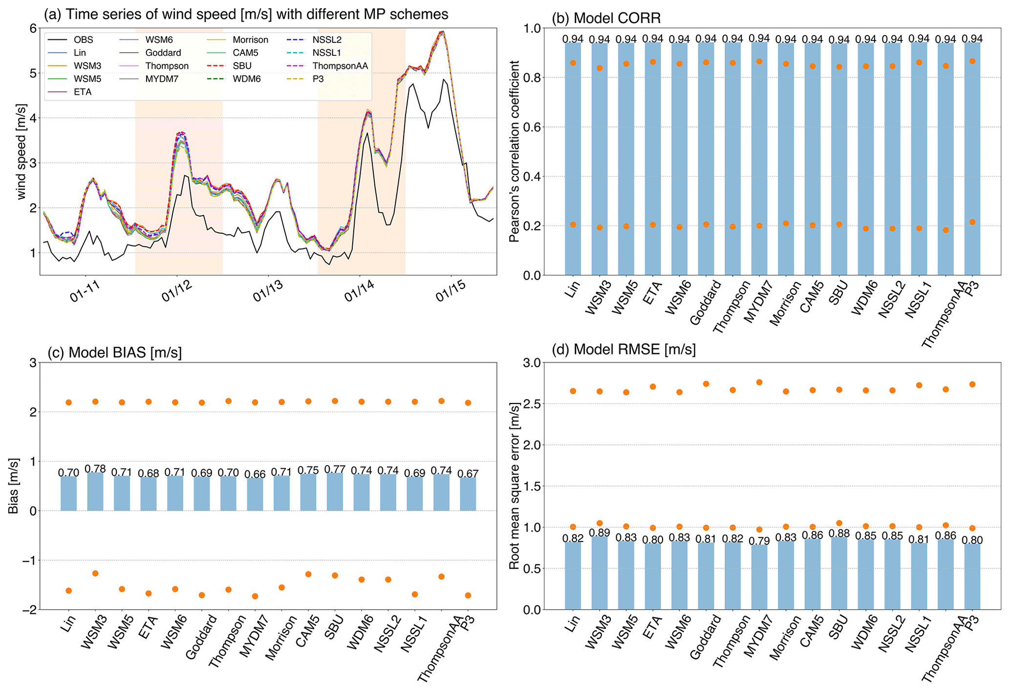
Figure 5 shows the time series of wind speed from the observations and simulations with different MP schemes. The simulations are similar, especially during 14–15 January 2019. The spread among simulations with different MP schemes is smaller than that with different PBL schemes, indicating that wind speed is less sensitive to the MP schemes. The CORR scores are very similar for all the MP schemes at a precision of 0.01, while MYDM7 is the best scheme according to the BIAS and RMSE scores, followed by P3 and ETA. The range of statistical scores across the stations is similar within different MP schemes, which provides a further indication of the low sensitivity of wind speed to MP schemes.

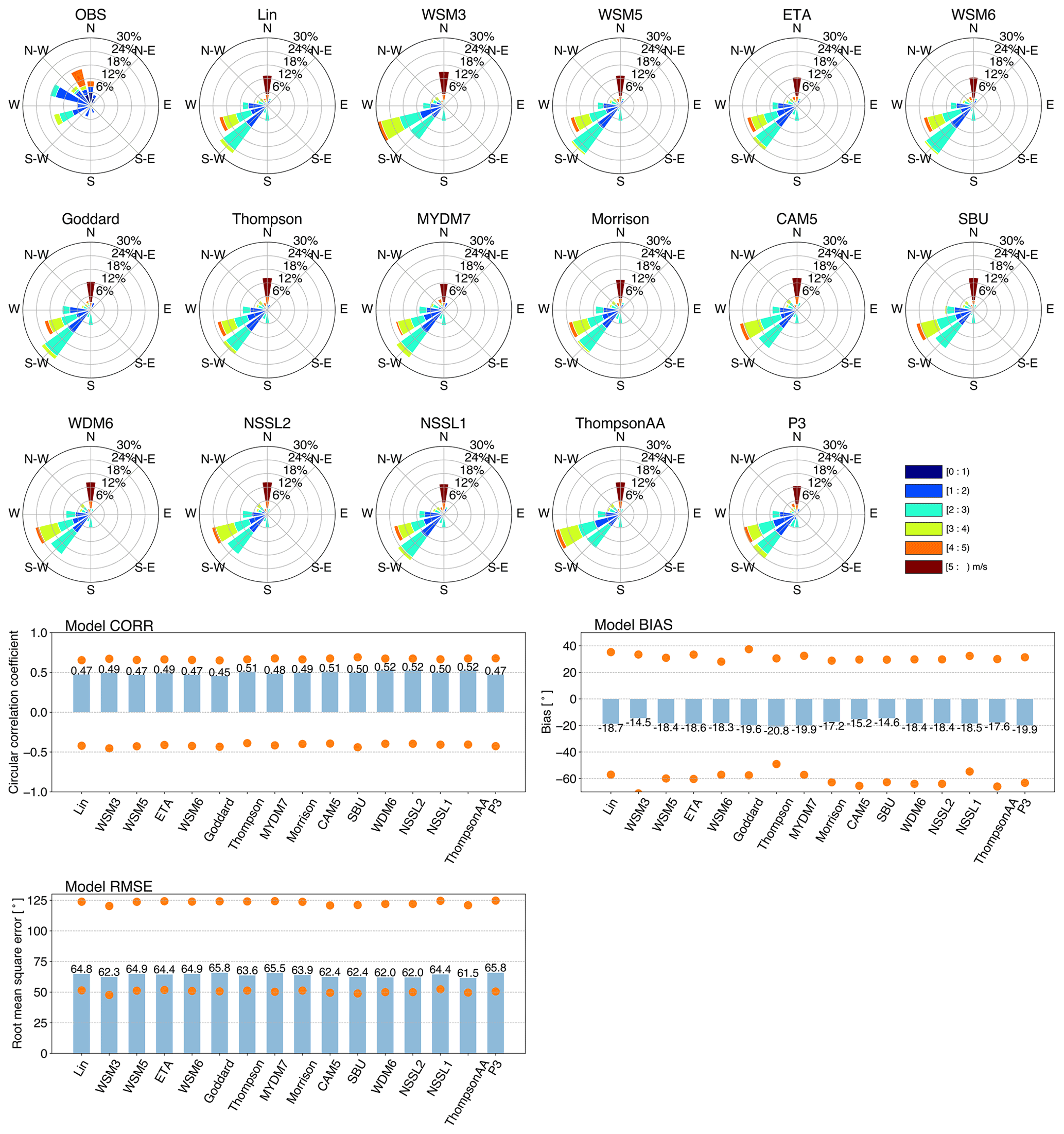
The sensitivity of wind direction to the MP schemes is also low, as the wind roses from simulations with different MP schemes are very similar (Fig. 6). WDM6, NSSL2 and ThompsonAA show the best CORR score of 0.52, followed by Thompson and CAM5. Meanwhile, WSM3 is the best scheme according to the BIAS score, and ThompsonAA is the best scheme according to the RMSE score.

Figure 6 Same as Fig. 4, but for the MP schemes.

3.1.3 Radiation

Figure 7 shows the time series of observed and simulated wind speed, the ensemble spread among different SW–LW schemes is larger than that with different MP schemes, but smaller than that with different PBL schemes, which indicates that simulated wind speed is more sensitive to the SW–LW schemes than the MP schemes and less sensitive to the PBL schemes. RRTMG and CAM show a larger overestimation than Dudhia–RRTM and Goddard at daytime peaks. The CORR scores are very similar for the SW–LW schemes at a precision of 0.01, and Dudhia–RRTM is the best scheme according to BIAS and RMSE scores, followed by Goddard.

Figure 7 Same as Fig. 3, but for the radiation schemes.

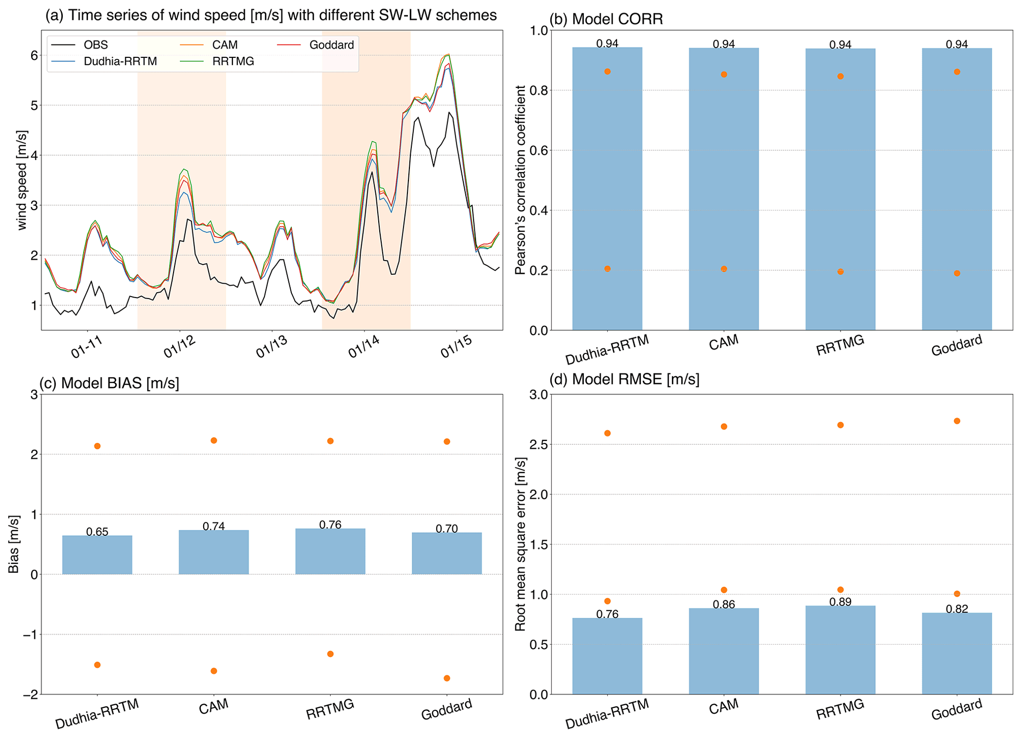
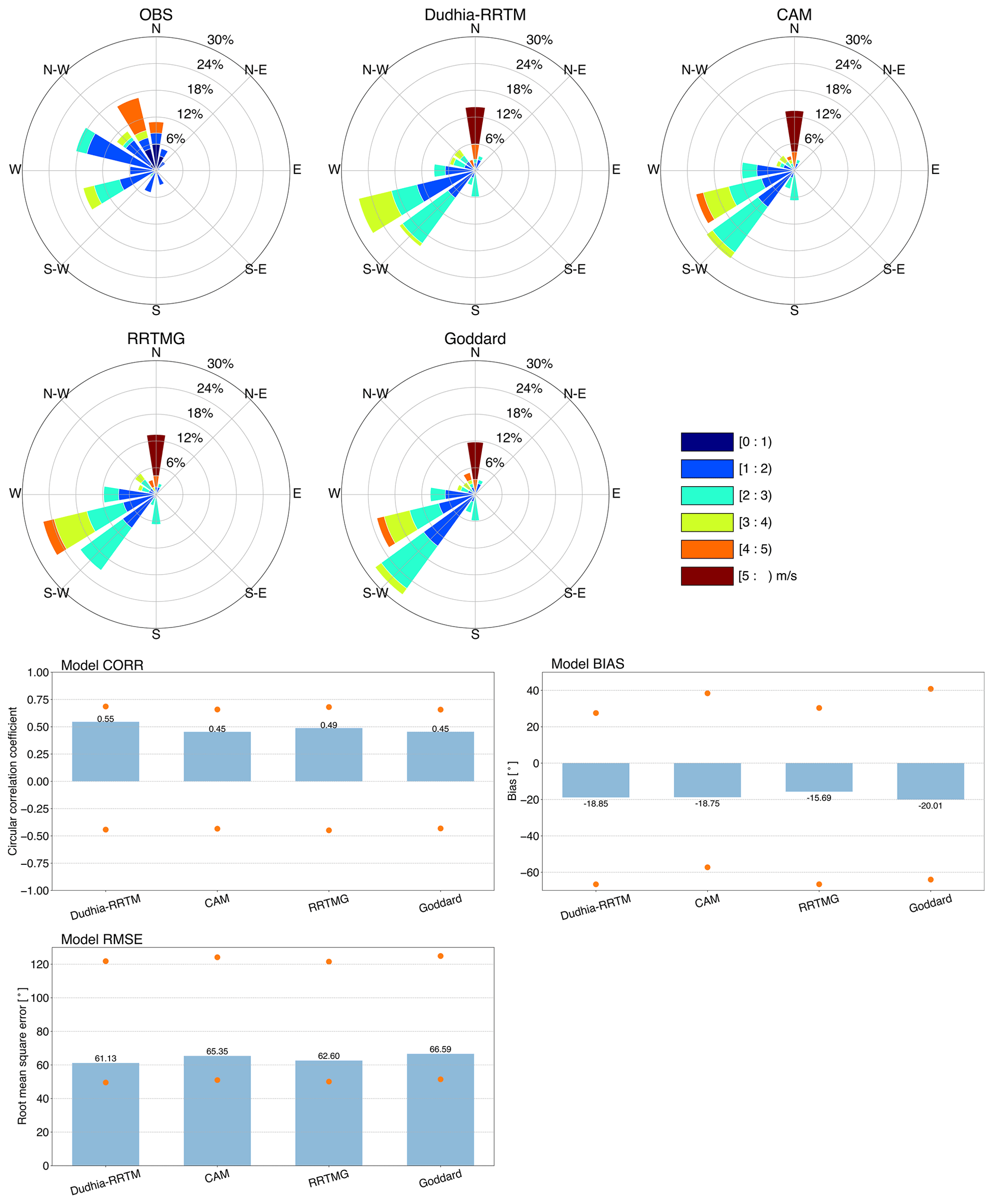
Figure 8 shows the wind roses during 11–15 January 2019 from simulations with different SW–LW schemes and the corresponding statistic scores. In simulations, wind is mostly from the southwest direction during the study period, which is different from the observation. According to the CORR score, Dudhia–RRTM is the best scheme with the highest value (0.55); meanwhile, the RRTMG scheme shows the best BIAS of −15.69^∘, and Dudhia–RRTM shows the best RMSE of 61.13^∘. As wind direction is more variable but less important under stable conditions with weak wind speed, the subsequent investigations mainly focus on wind speed.

Figure 8 Same as Fig. 4, but for the radiation schemes.

3.1.4 Interactions among parameterization schemes

Interactions among physical parameterizations also play an important role in wind simulation. Since it is not possible to show all possible combinations of PBL, MP, and SW–LW schemes in this study, the results of interactions between PBL and SW–LW schemes are selected as examples, which are illustrated in Fig. 9. The MP schemes used in the simulations are MYDM7 and P3, given that they show better performance in earlier investigations (see Sect. 3.1.2), and thus for each MP scheme, a total of 36 simulations (excluding QNSE) is illustrated. For wind speed simulations, the combination of MYJ and Dudhia–RRTM shows the best CORR, while the combination of YSU and Dudhia–RRTM ranks best according to BIAS and RMSE scores. For wind direction simulations, the combination of LES and Dudhia–RRTM shows the best CORR. According to BIAS and RMSE scores, the combination of TEMF and Dudhia–RRTM ranks best in MYDM7 case, and the combination of TEMP and RRTMG ranks best in P3 case.

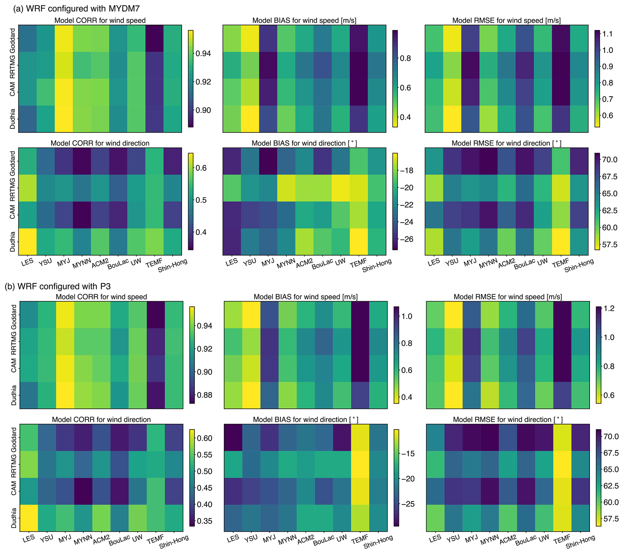
Figure 9 Statistic scores (CORR, BIAS and RMSE) for wind speed and direction for different combinations of PBL and SW–LW schemes, the MP schemes used in panels (a) and (b) are MYDM7 and P3, respectively. Dudhia represents Dudhia–RRTM SW–LW schemes in all the subplots.

Overall, for BIAS and RMSE scores of wind speed, within each PBL scheme, the same SW–LW group ranks best, and within each SW–LW group, the same PBL scheme ranks best. For example, no matter which SW–LW group, YSU is always the best, which indicate the good performance of YSU. However, it is worth noting that YSU shows pretty low BIAS (<0.4 m s⁻¹) and RMSE (<0.6 m s⁻¹) scores only when combined with the Dudhia–RRTM or Goddard schemes, when it is combined with RRTMG schemes, the BIAS and RMSE scores increase a lot. For the wind direction simulation, the pattern is different from that of wind speed. For example, for BIAS and RMSE scores, the best PBL scheme depends on the choice of SW–LW schemes, which indicates the influence of scheme interaction on model performance in wind direction simulations.

3.1.5 WRF configurations with the best individual performance

To determine the WRF configuration with the best individual performance, Taylor skill scores are calculated for wind speed within all simulations, the scores range from 0.2 to 1.0, with the best 10 WRF configurations having similar scores of about 1.0. The time series and statistics are illustrated in Fig. 10. The best 10 configurations have in common that they use the same PBL and SW–LW schemes, namely YSU and Dudhia–RRTM. This indicates a large impact of PBL and SW–LW on wind speed simulation compared with MP schemes and highlights the best performance of YSU and Dudhia–RRTM. Since Taylor skill score considers both correlation and standard deviation, the best scheme (i.e., WDM6) is not the scheme that has the best CORR (i.e., Goddard), BIAS (i.e., MYDM7 and ETA), or RMSE (i.e., Goddard, NSSL1, MYDM7 and ETA). In fact, there is no scheme that has all the best scores of CORR, BIAS and RMSE. Thus, model ensemble is needed to improve the performance. Figure 10 also illustrates the ensemble of different number of simulations, as well as a super ensemble of all 576 simulations (excluding QNSE). The result indicates that ensemble mean of four simulations with WDM6, Goddard, NSSL1 and MYDM7 MP schemes shows the best BIAS and RMSE scores. For the time series of wind speed (Fig. 10a), the spread of ENS(4) is significantly lower than that of ENS(576), and ENS(4) shows lower bias compared to ENS(576). According to the statistic scores, ENS(4) reduces model bias by approximately half compared to ENS(576), at the same time, the best individual schemes (NSSL1, MYDM7, P3 and ETA) can also reduce the bias by ∼50 %. It is worth to mention that the best CORR score of ENS(576) is also result of single model simulation with Goddard MP scheme. At the same time, the best BIAS score (0.33 m s⁻¹) is result of the single model simulation with MYDM7 or ETA, and the best RMSE score (0.52 m s⁻¹) is result of either the single model simulation with Goddard, NSSL1, MYDM7, or the ensemble using the three, four, or five best simulations.

Figure 10 (a) Time series of wind speed (m s⁻¹) from observation and different ensembles, and (b) CORR, (c) BIAS and (d) RMSE scores for the best 10 simulations along with different ensembles. The shadings in (a) represent the spread for ENS(4) and ENS(576). As the best 10 simulations use the same PBL (YSU) and SW–LW (Dudhia–RRTM) schemes, only the MP schemes are labeled in the figure.

3.2 Performance dependency on ocean proximity and elevation

Land surface conditions can affect the partitioning of sensible and latent heat fluxes, which impacts local low-level circulation patterns and wind distribution (Yu et al., 2013; Barlage et al., 2016). The weather stations in the study region were classified into different groups according to the ocean proximity and elevation.

3.2.1 Ocean proximity

Figure 11 compares the results of wind speed for coastal stations (closer than 5 km from the shoreline, 16 stations in total) and inland stations (over 5 km from the shoreline, 89 stations in total), the locations of these stations are shown in Fig. 1a. For both coastal and inland stations, the ensemble spread is the largest among the PBL schemes, followed by SW–LW and MP schemes, which is consistent with the results of the previous analysis in this study. WRF reproduces the time series of wind speed reasonably, with a larger overestimation for inland stations. The ensemble spread is larger for coastal stations compared with inland stations. As such, in addition to physical parameterizations, model performance is also influenced by ocean proximity.

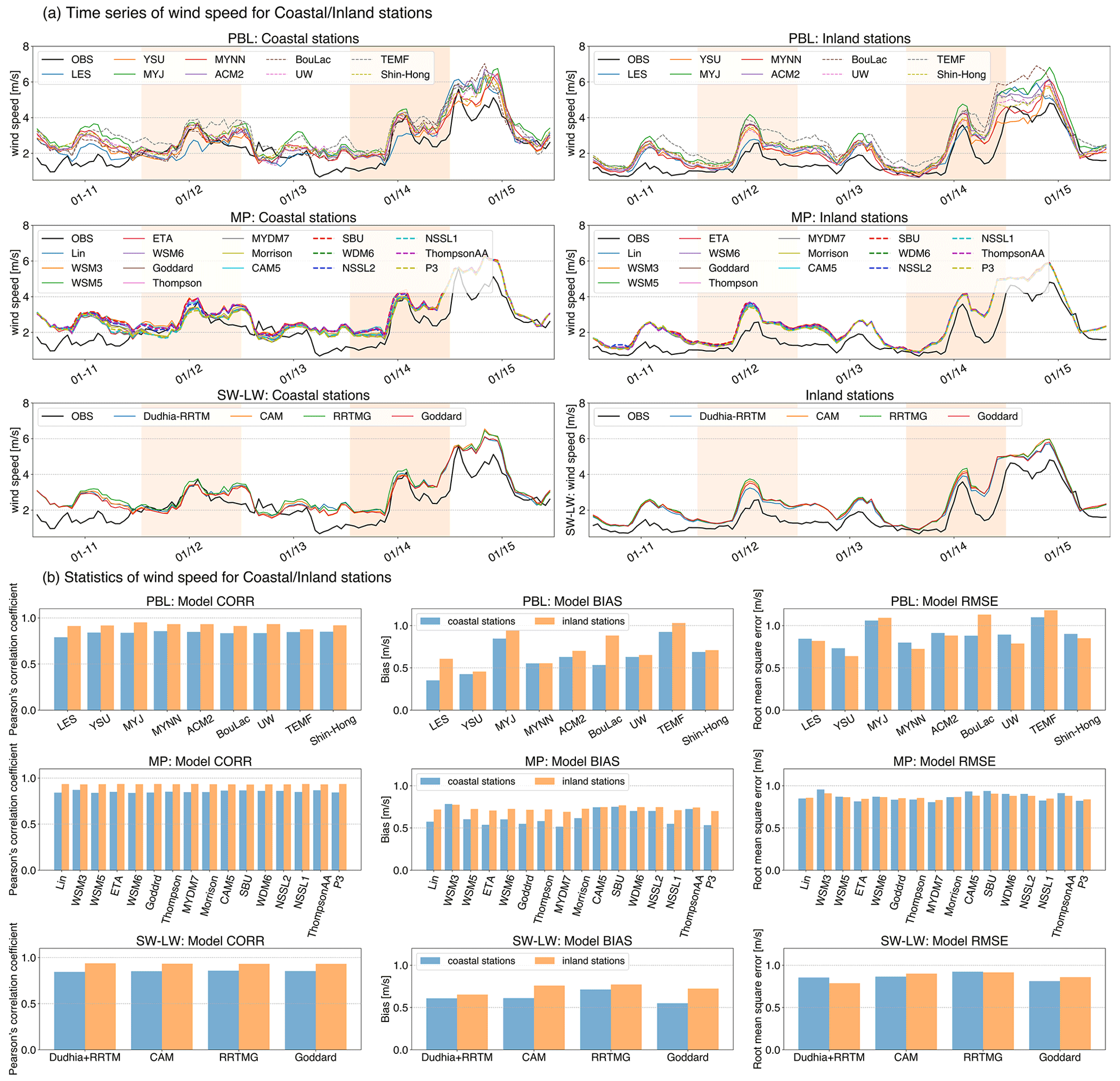
Figure 11 Comparison of simulated wind speeds between the coastal and inland stations shown in Fig. 1a as well as the corresponding statistical scores.

The statistical scores are also illustrated in Fig. 11, the CORR scores are consistently lower for coastal stations compared to inland stations, and the BIAS scores are generally worse for the inland stations. Thus, the model performance tends to degrade for the inland stations according to the BIAS scores.

Our comparison indicates that the parameterization schemes with the best performance for inland stations are generally consistent with those of previous investigations for all the stations in this study, as most of the stations are inland stations (89 out of 105 stations). However, for coastal stations, the results are different. For instance, MYNN shows the best CORR score among the PBL schemes, while LES (YSU) shows the best BIAS (RMSE) score. For the SW–LW schemes, Goddard shows the best CORR, BIAS, and RMSE, while Dudhia–RRTM ranks worst according to the CORR score.

3.2.2 Elevation

Figure 12 shows the comparison for stations with different elevation (e.g., <50 m, 51 stations in total; >50 and <250 m, 36 stations in total; >250 m, 19 stations in total). Observation shows that peak wind speed decreases with increasing elevation during the study period; for example, the peak observed wind speed of high-elevation stations (>250 m) is 1.5 m s⁻¹, slower than that of low-elevation stations (<50 m). However, the peak simulated wind speed is generally similar for stations with different elevations, which bring larger model errors for the high-elevation stations. Further investigations are needed to reveal the underlying mechanisms for lower wind speeds of high-elevation stations and the mismatch between observations and model simulations. As shown by the statistical scores, for all PBL, MP, and SW–LW schemes, CORR generally decreases with increasing elevation, while BIAS and RMSE scores increase with elevation, and thus the evaluation metrics tend to degrade with increasing elevation under stable conditions over the study area. For different parameterization types, the scheme with the best performance is generally similar, with different elevations; e.g., for PBL schemes, MYJ is always the best at all elevation categories according to CORR, and YSU always ranks best according to the BIAS and RMSE scores.

Figure 12 Comparison of simulated wind speeds (m s⁻¹) for stations <50 m (51 stations in total), >50, and <250 (36 stations in total), and >250 m (19 stations in total) and the corresponding statistic scores.

3.3 Comparison of simulations with different model performances and the effects of other model options

In order to evaluate atmospheric properties that are crucial for air quality under stable conditions and to investigate what drives the differences in wind speed, we compare the simulated wind field from the simulation with the best Taylor skill score (i.e., using the YSU, Dudhia–RRTM, and WDM6 schemes) and the station observations; meanwhile, the same simulation but with the QNSE PBL scheme (i.e., using the QNSE, Dudhia–RRTM, and WDM6 schemes) is used for comparison between the simulations with good and poor performances. In addition, the impacts of the land surface model, surface layer scheme, and different options in the YSU scheme are also investigated in this section.

3.3.1 Spatial distribution of the wind field

Figure 13 compares the spatial distribution of observed and simulated wind fields during the study period, and we choose 14:00 LT as an example. The simulation with the best Taylor skill score is referred to as YSU, and the simulation using the QNSE PBL scheme is referred to as QNSE. YSU generally reproduces the wind field in the study area, especially in terms of wind speed. For example, the observed wind speed is lower on 13 January 2019, with values lower than 2 m s⁻¹ for many stations, while on 15 January 2019, the observed wind speed is higher than 4 m s⁻¹ for most stations. In the simulation using YSU, wind speed is about 2 m s⁻¹ on 13 January 2019 and is higher than 4 m s⁻¹ on 15 January 2019 over the study area, which is similar to the observation. By contrast, simulation with QNSE fails to reproduce the distribution of wind speed and shows strong overestimation, especially over the mountain areas of the study area; for example, the peak wind speed in simulation with QNSE exceeds 20 m s⁻¹ on 15 January 2019, which is more than 5 times greater than the observation. This overestimation is consistent with the large positive bias in previous investigations of Fig. 3. For the wind direction simulation, YSU shows degraded performance compared to wind speed and generally fails to reproduce the wind direction distribution for most of the stations, which is also the case for QNSE.

Figure 13 Spatial distribution of simulated (black vector) and observed (red vector) winds at 14:00 LT during the study period from simulations with the YSU and QNSE schemes; the shading indicates the elevation, and the height of the wind is 10 m.

3.3.2 Vertical profile of wind speed

Figure 14 shows the observed and simulated vertical profiles of wind speed at 08:00 and 20:00 LT during the study period, and the location of the sounding station is illustrated in Fig. 1. YSU reproduces the vertical structure of wind speed reasonably; for example, within the low levels below 2.5 km, the simulated wind speed from the YSU scheme is similar to the observation, with model bias lower than 2.5 m s⁻¹ in most cases. Meanwhile, QNSE shows a worse performance in reproducing the vertical structure of wind speed, with a large model bias compared to YSU. QNSE overestimates the wind speed by almost 20 m s⁻¹ at 20:00 LT, 11 January 2019, and by 30 m s⁻¹ at 20:00 LT, 12 January 2019. It is interesting to note that, at 08:00 LT, the simulations using QNSE show smaller differences than that using YSU, and thus the largest differences between YSU and QNSE generally occur at a specific time during the study period, which is also revealed in Fig. 3a.

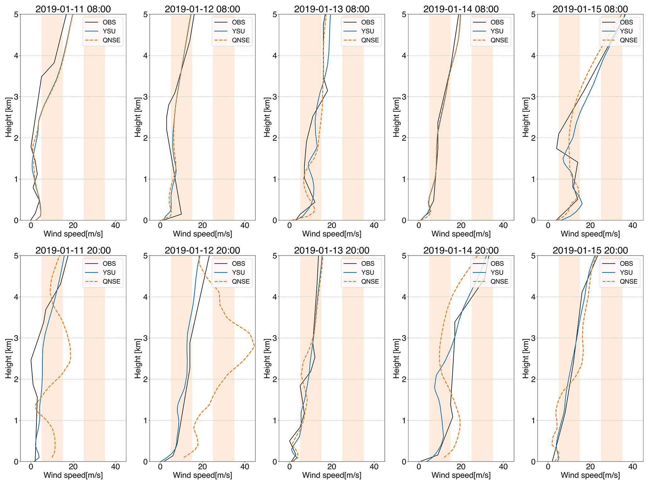
Figure 14 Wind speed profile from observations and simulations with the YSU and QNSE schemes at 08:00 and 20:00 LT during the study period.

3.3.3 Impact of land surface models

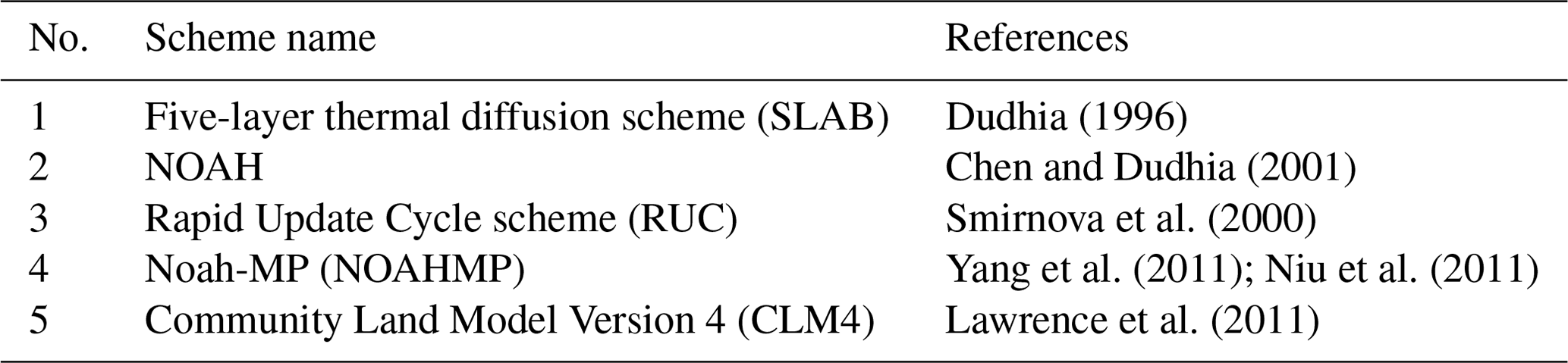
Figure 15 shows the evaluation of different land surface models (LSMs); only five simulations were conducted using the model configurations with the best Taylor skill score (i.e., YSU in Sect. 3.3.1), and except for the LSM schemes, the LSMs (i.e., SLAB, NOAH, RUC, and NOAHMP) investigated are listed in Table 3. The simulations reproduce the time series of wind speed well, with a larger spread during 14–15 January 2019. NOAHMP and CLM4 show the best CORR score of 0.93, and NOAH is slightly worse according to this score. Meanwhile, NOAHMP ranks best according to the BIAS and RMSE scores, followed by the RUC scheme. Thus, NOAHMP shows the best performance among different LSMs in wind speed simulations in this study. However, the large difference among LSMs indicates that we should take land surface parameterizations into consideration in future studies.

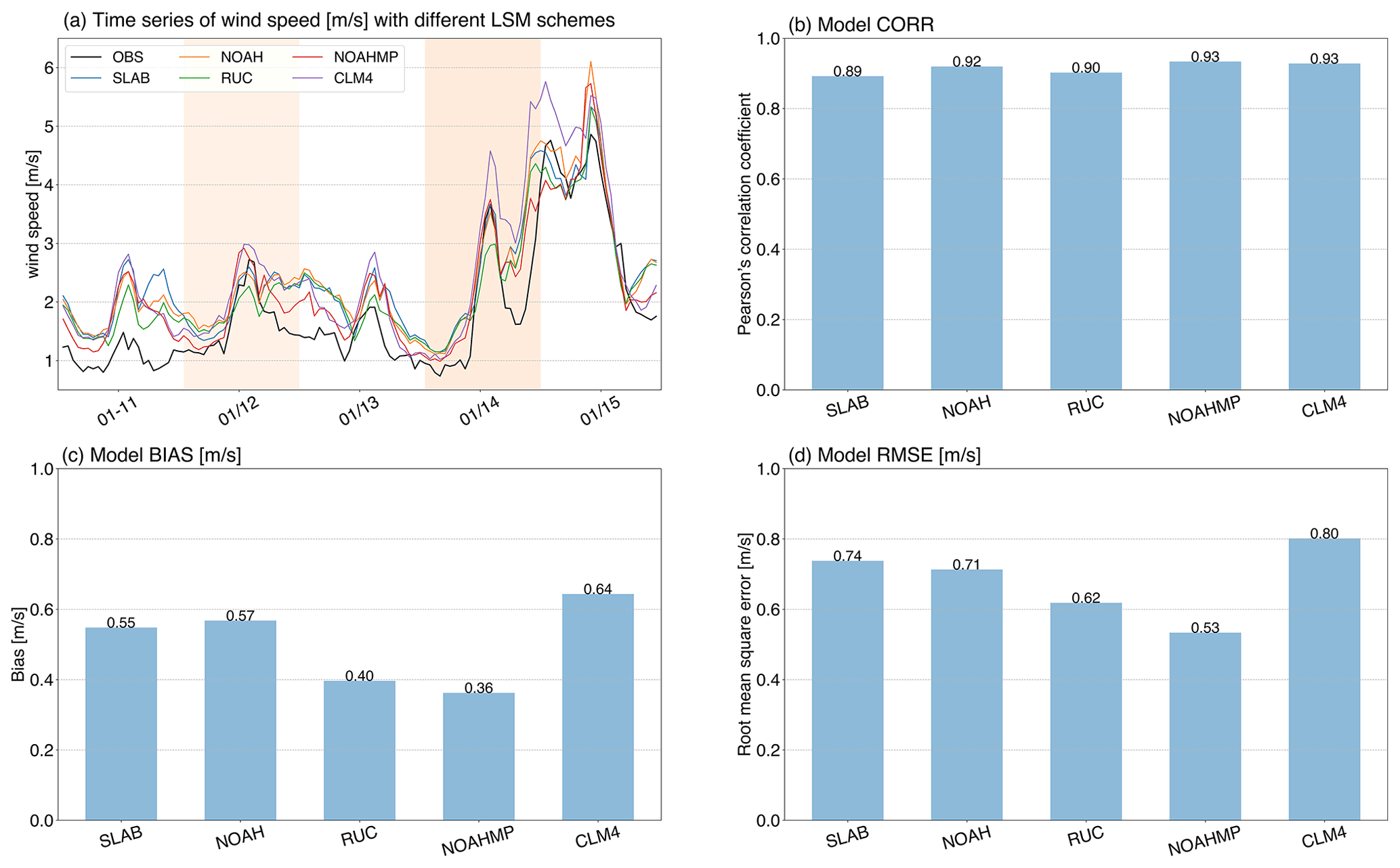
Figure 15 Same as Fig. 3 but for simulations with different land surface schemes. The PBL, MP, and SW–LW schemes used are the same as the simulation with the best Taylor skill score (WDM6 in Fig. 10).

Table 3 List of land surface models investigated in this study.

3.3.4 Impact of surface layer schemes

In the WRF model, the surface layer (SL) schemes are somehow binding with PBL schemes, and it is not possible to run all PBL schemes with the same SL scheme. However, it is meaningful to conduct simulations using a specific PBL scheme that can work with multiple SL schemes to investigate the effect of SL schemes on wind simulation. Figure 16 compares the simulation results of different SL (MM5, Janjic, GFS, MYNN, and PX, Table 4) schemes using UW as the PBL scheme, and the other model configurations are the same as the simulation with the best Taylor skill score. Simulations with different SL schemes generally reproduce the time series of wind speed well, with CORR scores of about 0.93 for most schemes. However, all simulations overestimate the wind speed, especially for the Janjic scheme. At the same time, according to the BIAS and RMSE scores, MYNN shows the best performance, followed by the GFS and PX schemes. Thus, the SL schemes also have a major influence on the wind simulation.

Figure 16 Same as Fig. 3 but for simulations with different surface layer schemes.

Table 4 List of surface schemes investigated in this study.

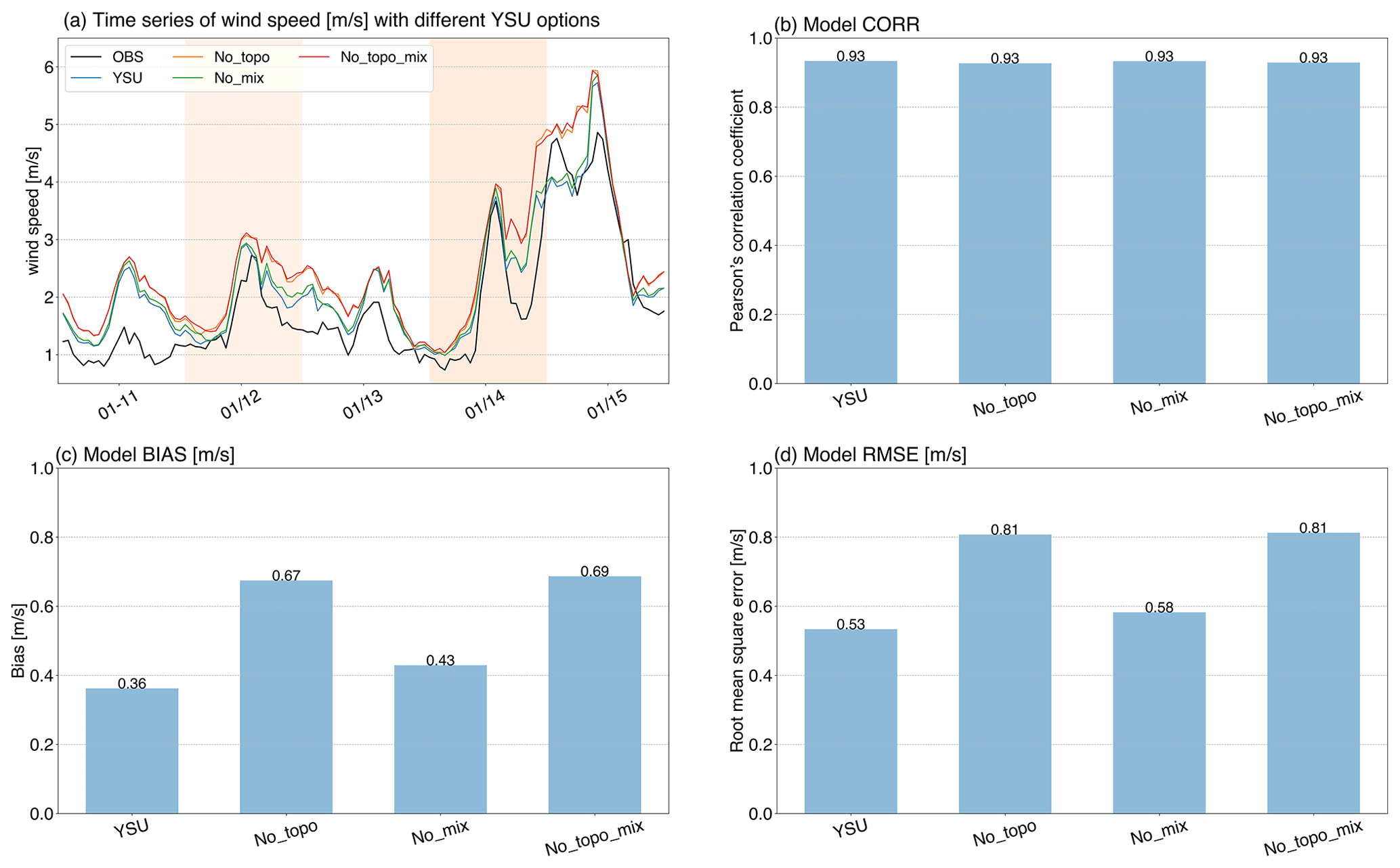
3.3.5 Impact of options in the YSU scheme

The impact of different options in YSU on wind-speed simulation is illustrated in Fig. 17, the simulation with the best Taylor skill score is referred to as YSU, and three extra simulations with top-down mixing option turning off (No_mix), topographic correction with option turning off (No_topo), and both options turning off (No_topo_mix) were conducted for comparison. The simulated wind speed increases when we turn off the individual or both options, which enlarges the overestimation of wind speed under stable conditions in our study (Fig. 15a). Turning off the two options in YSU degrades the model performance with worse evaluation metrics. For example, the BIAS score increases from 0.36 to 0.67 m s⁻¹ in No_topo, to 0.43 m s⁻¹ in No_mix, and to 0.69 m s⁻¹ in the No_topo_mix simulation. At the same time, RMSE scores show similar degradation when turning off the options in YSU.

Figure 17 Same as Fig. 3 but for simulations with different YSU options.

4 Summary and discussion

In this study, we investigate wind simulations under stable conditions when a haze event affected North China. Surface meteorological observations are used to evaluate the WRF model's ability to reproduce the evolution of winds during the event. The grid spacing of 0.5 km used in this study belongs to the PBL gray zone resolution, which has rarely been used in previous simulation studies in China, and thus the results of this study provide a valuable reference for other simulations over North China. A number of WRF sensitivity experiments (640 in total) are conducted, altering the PBL, MP, and SW–LW schemes to determine the sensitivity of wind speed and direction simulations to model physical parameterizations. Further investigations considering the ocean proximity, elevation, and other model options are conducted to provide deeper insight into the factors that influence model sensitivities.

In general, the WRF model reproduces the temporal variation of wind speed over the study area well, and the spread in wind speed is largest within the PBL schemes tested, followed by SW–LW, and then the MP schemes. The wind direction is notably worse reproduced by WRF compared to wind speed. This result is consistent with the findings of previous simulations performed in other locations (Dzebre and Adaramola, 2020; Gómez-Navarro et al., 2015; Santos-Alamillos et al., 2013).

Among all PBL schemes, MYJ shows the best CORR score of 0.96, and MYNN, ACM2, and UW are slightly worse according to this score. YSU is the best scheme according to the BIAS and RMSE scores (0.45 and 0.61 m s⁻¹), followed by MYNN (0.55 and 0.70 m s⁻¹). For the SW–LW and MP schemes, the CORR scores are similar, and Dudhia–RRTM and MYDM7 show the best model performances out of all the SW–LW and MP schemes according to the BIAS and RMSE scores. The simulation using the YSU PBL, WDM6 MP and Dudhia–RRTM SW–LW schemes shows the best performance, with the highest Taylor skill score. Interactions among the physical parameterization schemes also play an important role in wind simulations, as the best verification scores can be achieved by a certain combination of schemes. The ensemble mean of all the simulations shows the highest CORR core in wind speed, while the 10 best simulations show much better performance than the ensemble in terms of BIAS and RMSE.

The schemes with the best performances for inland stations are consistent with the results of all the stations, as the majority of stations are inland stations; however, for coastal stations, MYNN is the best scheme among all PBL schemes according to CORR, while LES (YSU) shows the best BIAS (RMSE) score. For SW–LW schemes, Goddard schemes show the best scores of CORR, BIAS, and RMSE, while Dudhia–RRTM schemes rank worst according to the CORR score. The schemes with the best performance are similar to different elevations for different parameterization types; however, model performance tends to degrade with increasing elevation.

As in our study, the model ensemble does not always provide the best performance and model post-processing, and the bias correction techniques are especially needed to be taken into consideration, which can significantly reduce the systematic errors in model simulation. In addition, the PBL schemes play a dominant role in wind simulation, and further tuning of the parameters within the PBL schemes, such as the turbulent kinetic energy (TKE) dissipation rate, TKE diffusion factor, and turbulent length-scale coefficients, is needed. In addition to the PBL and SW–LW schemes, the LSM and SL schemes also have a non-negligible influence on the wind simulation, which should be taken into consideration in future studies. Finally, it is worth pointing out that the presented findings in this study could be unique to the meteorological setup of the event, the location, the input dataset, the domain setup, and other unchanged parameterization types or model settings.