A tool for air pollution scenarios (TAPS v1.0) to enable global, long-term, and flexible study of climate and air quality policies

Air pollution is a major sustainability challenge – and future anthropogenic precursor and greenhouse gas (GHG) emissions will greatly affect human well-being. While mitigating climate change can reduce air pollution both directly and indirectly, distinct policy levers can affect these two interconnected sustainability issues across a wide range of scenarios. We help to assess such issues by presenting a public Tool for Air Pollution Scenarios (TAPS) that can flexibly assess pollutant emissions from a variety of climate and air quality actions, through the tool's coupling with socioeconomic modeling of climate change mitigation. In this study, we develop and implement TAPS with three components: recent global and fuel-specific anthropogenic emissions inventories, scenarios of emitting activities to 2100 from the MIT Economic Projection and Policy Analysis (EPPA) model, and emissions intensity trends based on recent scenario data from the Greenhouse Gas–Air Pollution Interactions and Synergies (GAINS) model. An initial application shows that in scenarios with less climate and pollution policy ambition, near-term air quality improvements from existing policies are eclipsed by long-term emissions increases – particularly from industrial processes that combine sharp production growth with less stringent pollution controls in developing regions. Additional climate actions would substantially reduce air pollutant emissions related to fossil fuel (such as sulfur and nitrogen oxides), while further pollution controls would lead to larger reductions for ammonia and organic carbon (OC). Future applications of TAPS could explore diverse regional and global policies that affect these emissions, using pollutant emissions results to drive global atmospheric chemical transport models to study the scenarios' health impacts.

1 Introduction

Air pollution is an urgent global health threat, with similar sources to the greenhouse gas (GHG) emissions that drive climate change (Murray and GBD 2019 Risk Factors Collaborators, 2020). Fine particulate matter (PM_2.5) from fossil fuels and other human sources may have caused millions of premature deaths in recent years (McDuffie et al., 2021; Lelieveld et al., 2019), while ground-level ozone can increase mortality risk, exacerbate crop loss, and worsen socioeconomic disparities (Saari et al., 2017; Turner et al., 2016; Sampedro et al., 2020a). Projecting these impacts requires future scenarios for those air pollutants' precursor emissions – but more flexible and accessible tools are needed to elucidate the interdependent but distinct effects of economic, climate, and pollution policy on air quality and human health.

Many research efforts focus on the health “co-benefits” of reduced air pollutant emissions from mitigating GHG emissions (Gallagher and Holloway, 2020; Karlsson et al., 2020; Nemet et al., 2010; Rao et al., 2016; Sampedro et al., 2020b). Studies have found that the near-term health benefits from GHG reductions can be on par with or even greater than their near-term climate benefits (Markandya et al., 2018; Shindell et al., 2021). Health benefits vary strongly by region and sector (Vandyck et al., 2020), highlighting the importance of granular analyses and actions that prioritize reductions in high-emitting areas (Polonik et al., 2021). As such, climate action must be complemented by pollution-specific policies to maximize air quality benefits (Reis et al., 2022; Tong et al., 2021), prompting calls for combined policy assessments to address both issues together (Selin, 2021; Vandyck et al., 2021).

For studies that do vary both climate and air quality policies, most use one of a few existing scenario sets. Current options include the shared socioeconomic pathways (SSPs), a set of global scenarios to 2100 that treat climate and air pollution separately but tie the latter to specific societal narratives (O'Neill et al., 2017; Riahi et al., 2017). Each SSP is associated with a specific pollution control ambition, with regional emissions intensity trends that depend on affluence levels (Rao et al., 2017). These trends were derived from two scenarios developed with the widely used Greenhouse Gas–Air Pollution Interactions and Synergies (GAINS) model: current legislation (CLE), which assumes compliance with existing source- and region-specific emission limits, and the maximum feasible reduction (MFR) case, which assumes gradually increasing application of the lowest-emitting currently available technologies (Amann et al., 2011; Klimont et al., 2017). The resulting air pollutant emission trajectories are included in the sixth Coupled Model Intercomparison Project (CMIP6) and presented online (Riahi et al., 2020; Rogelj et al., 2018).

Other approaches have a different scope of economic assumptions, timescales, or pollutant species. While several studies vary climate and air quality scenarios across pollutants, they often project emissions intensities based on income rather than policy (Radu et al., 2016; Scovronick et al., 2019). Others have begun to internalize climate–health–economic linkages into optimal policy pathways (Reis et al., 2022), while still using SSP pollution assumptions as baselines. Studies in the Energy Modeling Forum (EMF)-30 use the GAINS scenarios more directly, focusing on black carbon (BC) and organic carbon (OC) (Smith et al., 2020) or non-agricultural pollutants through 2050 (Vandyck et al., 2018). Since then, GAINS has been updated with more nuanced regions, sectors, and emissions trends (GAINS Developer Team, 2021a), such as recent SO₂ (Zheng et al., 2018) and black carbon (Kanaya et al., 2020) reductions in China, as well as revised data and SSP-consistent modeling for the waste management sector (Gomez Sanabria et al., 2022).

Some recent studies have used this updated GAINS model to explore more near-term results or policy extremes. Rafaj et al. (2021) use several integrated assessment models (IAMs) to assess health impacts around current climate policies, proposed policies, or likely attainment of the Paris Agreement's temperature targets (through 2050), applying GAINS CLE and MFR to the 1.5 ^∘C case while maintaining CLE otherwise. Amann et al. (2020) develop a “Clean Air” scenario that includes additional climate, energy, agriculture, and food policies, finding that those additional policies (beyond traditional air pollution controls of GAINS) would lead to nearly double the benefits of reduced PM_2.5 exposure. Hamilton et al. (2021) use a related scenario of “health in all climate policies”, including air pollution reductions, diet change, and active travel benchmarks in nine selected countries. Both these latter papers focus on aggregate effects (comparing base cases to scenarios of those policy levers combined together), and are limited geographically (Hamilton et al., 2021) or temporally to 2040.

We aim to present a more flexible model-based capacity for long-term global scenarios, allowing the user to specify diverse levels of climate actions and pollution controls to estimate their combined effect on air pollutant precursor emissions. The resulting Tool for Air Pollution Scenarios (TAPS) can efficiently assess a wide range of climate and air quality policy pathways – from broad to specific at the regional, sectoral, and fuel-based level. In addition, its emissions outputs can provide flexibility for different air quality and health analyses – whether using emulators for rapid scenario study, or driving global atmospheric chemical transport models (CTMs) that avoid emulators' precalculated emissions-to-impact relationships. We demonstrate the tool with illustrative scenarios after coupling with the Economic Projection and Policy Analysis model version 7 (EPPA7). EPPA is a global multi-region multi-sector recursive–dynamic computable global equilibrium (CGE) model that has been used to study a variety of climate and economic policy impacts (Chen et al., 2015, 2017; Paltsev et al., 2005). EPPA7 is a recent version that includes updated economic data as well as new representations of advanced energy technologies (Chen et al., 2022). While prior efforts have sought to endogenize EPPA's air pollutant emissions trends based on the cost of pollution control options (Sarofim, 2007; Valpergue De Masin, 2003; Waugh, 2012), these internal estimates have been limited to select studies (Nam et al., 2013). In contrast, the TAPS framework combines EPPA's energy and land use outputs with other data to produce its own pollutant emissions scenarios, allowing it to be exercised autonomously for flexible scenario development (Fig. 1).

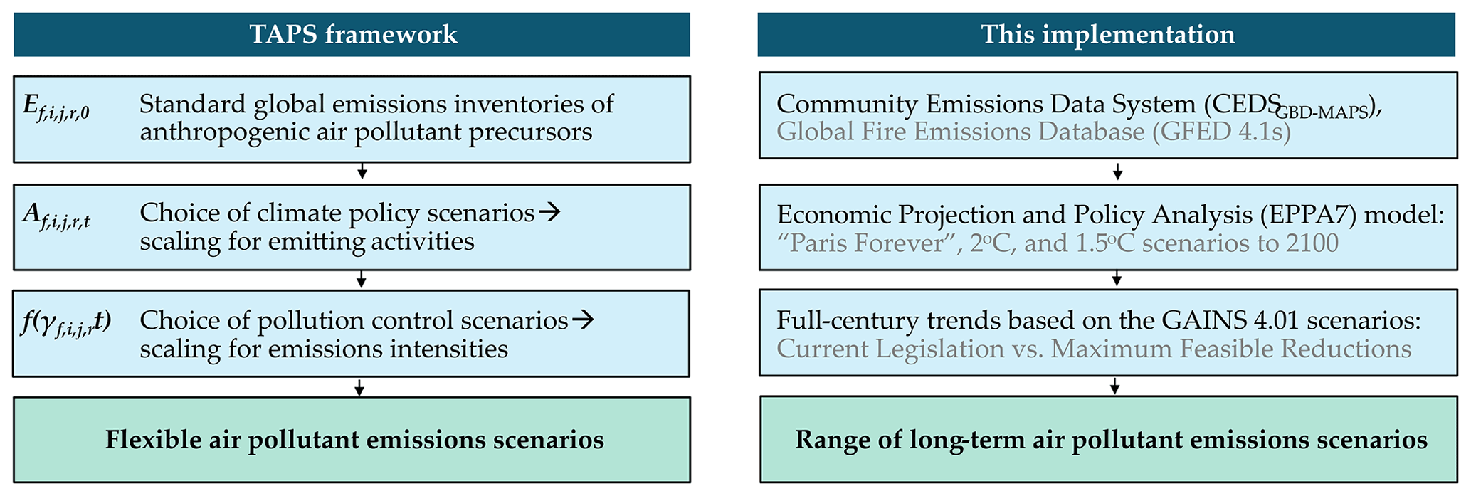
Figure 1 Summary of the Tool for Air Pollution Scenarios (TAPS) framework and implementation here, based on climate policy scenarios in EPPA7 and pollution control scenarios from the Greenhouse Gas–Air Pollution Interactions and Synergies (GAINS) model. Emissions trends are specific to each fuel f, pollutant species i, sector j, region r, and time point t in the inventories and EPPA7 scenarios used.

First, we utilize emissions inventories that are well-suited for atmospheric modeling work on health impacts – following the sources of SSPs but with updated estimates. Next, we scale those emissions by fuel-specific activities in EPPA, using climate policy scenarios from the global CGE model with full-century time horizons that are longer than most comparable works. Finally, we use updated emissions intensity scenarios from GAINS to assess policies specific to air pollution – while designing pathways that allow for potential future innovation beyond today's technology options. The following section will describe these steps in turn, before comparing results to SSP benchmarks and discussing next steps for tool refinement and health applications.

2 Methodology

Our estimates of air pollutant emissions involve three main inputs: a base-year emissions inventory (Sect. 2.1), a projected trend in energy use and other polluting activities (Sect. 2.2), and a projected trend in emissions intensity (Sect. 2.3). The following equation (based on Fig. 1) summarizes these components:

$$\begin{array}{}\text{(1)}& E_{f,i,j,r,t}=E_{f,i,j,r,\mathrm{0}}\times A_{f,i,r,t}\times f\left({\mathit{\gamma }}_{f,i,j,r}t\right),\end{array}$$

where the emissions $E_{f,i,j,r,t}$ of inventory fuel f, inventory sector i, pollutant species j, EPPA region r, and time t are calculated as the product of base-year emissions $E_{f,i,j,r,\mathrm{0}}$, fuel-specific activity $A_{f,i,j,r,t}$, and the function $f\left({\mathit{\gamma }}_{f,i,j,r}t\right)$ in scenario-specific emissions intensity over time. The below sections discuss each of these components in more detail, as well as the specific scenarios shown in this analysis (Sect. 2.4).

Public versions of the tool, outputs, and underlying data are described in the code and data-availability section (including processes for figure reproduction). To facilitate coupling with global atmospheric CTMs for health impact analysis, we also include the capability to produce gridded outputs for emissions scaling – following the inventory's spatial distribution as done for the SSPs (Feng et al., 2020). Inputs and Python code can be downloaded and modified to explore the effects of different climate or air quality policies at the region, sector, or fuel-based level. While it is simplest to construct scenarios that maintain the structure of current data sources (adjusting from Sect. 2.4), future applications of TAPS could theoretically be extended to other inventories or policy model outputs if the database-integration steps were completed (adjusting from Sect. 2.1–2.3).

2.1 Base-year emissions inventory

This paper uses base-year emissions from the Community Emissions Data System's Global Burden of Disease Major Air Pollution Sources project (CEDS_GBD-MAPS; https://doi.org/10.5281/zenodo.3865670, McDuffie et al., 2020c), an updated version of the anthropogenic air pollutant emissions inventory used in the SSPs as well as atmospheric modeling of health impacts (GEOS-Chem, 2021). The CEDS is a global inventory that includes sulfur dioxide (SO₂), carbon monoxide (CO), ammonia (NH₃), black carbon (BC), organic carbon (OC), nitrogen oxides (NO_x), and 23 separate non-methane volatile organic compounds (NMVOC). It offers monthly data globally on a 0.5^∘ × 0.5^∘ grid for 1750–2014 (Hoesly et al., 2018), with updates for 1970–2017 (McDuffie et al., 2020a) that divide each of 11 sectors into 4 fuel categories (Table A1). Compared to subsequent versions with fewer sectors and no fuel separation, we use the version in McDuffie et al. (2020a) because it combines fuel-specific granularity with emissions totals that largely match the latest trends in https://github.com/JGCRI/CEDS (last access: 5 October 2022) (such as lower BC and OC totals). We use 2014 emissions to match the economic base-year of the GTAP10 database (Aguiar et al., 2019) used in EPPA7 (as described in Sect. 2.2).

We also include emissions of agricultural waste burning, the only type of open burning represented in EPPA's economic activities (Chepeliev, 2020). We follow the SSPs (van Marle et al., 2017) and GEOS-Chem model (GEOS-Chem, 2021) by using emissions from the Global Fire Emissions Database (GFED) version 4.1s at a 0.25^∘ × 0.25^∘ grid (van der Werf et al., 2017). Although the GFED gives emissions estimates in terms of dry matter rather than specific pollutants, we use emission factors based on Akagi et al. (2011) to convert these estimates to pollutant-specific emissions, as recommended by the GFED and done for the SSPs (see van Marle et al., 2017, Table C1). We use 2014 values to match the base year of EPPA7; 2014 GFED emissions are generally consistent with emissions quantities from neighboring years. We do not include emissions from wildfires, non-anthropogenic sources, or other burning sources in GFED (given their lack of representation in EPPA and GAINS). Other fire emissions could be added from GFED or similar inventories after deciding on their future trajectories (which we leave to later work, given large uncertainties). In addition, we do not currently include aviation emissions, given their exclusion from both CEDS_GBD-MAPS and GAINS. Air pollution from global aviation has been linked to 16 000 annual deaths (Eastham and Barrett, 2016), or less than 1 % of pollution's estimated global mortalities (Murray et al., 2020). However, future efforts could consider sources such as the 2019 version of the Aviation Emissions Inventory Code (AEIC; Simone et al., 2013), as used in the GEOS-Chem model (GEOS-Chem, 2021).

2.2 Projecting emitting activities

2.2.1 Choice of economic data source

This paper uses full-century activity outputs from several of EPPA's global climate policy scenarios. The latest version of the EPPA model (EPPA7) has 18 regions of the world and 14 economic sectors, as summarized in Appendix B (Paltsev et al., 2021). To scale the base-year emissions inventories by future trends in EPPA, we perform sectoral mapping from each of the 12 inventory sectors (11 from CEDS_GBD-MAPS plus agricultural waste burning from GFED) to 1 or more of the EPPA7 sectors (Table 1). The process is based on comparisons of CEDS sectors with GTAP10 (Chepeliev, 2020) and its transferal to EPPA sectors, using standard Intergovernmental Panel on Climate Change (IPCC) definitions as a common reference point (Table D1). Since EPPA lacks direct matches for “Waste”, “Solvents”, or the “Residential” emissions that are often from solid biofuels in CEDS, we use population to scale these sectors. Despite its approximations, this sectoral mapping is useful to keep emissions projections in terms of CEDS and GFED sectors, facilitating SSP comparisons and future atmospheric modeling applications.

2.2.2 Choice of activity parameters

Next, we select fuel-specific parameters to scale each emitting activity based on the approach used in the similar US Regional Energy Policy (USREP) model (Yuan et al., 2019). In USREP, emissions from fuel consumption are mostly scaled by future sectoral energy consumption, while non-combustion sources are scaled by that sector's economic output (Dimanchev et al., 2019; Thompson et al., 2014). Here, we apply a similar method to EPPA as described in Table 1, using the four fuel categories (three for combustion, one for “process”) in CEDS_GBD-MAPS. Each source's scaling is based on the proportion of its base-year emissions (Table A1) as follows:

$$\begin{array}{}\text{(2)}& A_{f,i,j,r,t}={\displaystyle \frac{E_{f,i,j,r,\mathrm{0}}}{E_{i,j,r,\mathrm{0}}}}\times {\sum }_{\mathrm{Ei}}{A}_{f,\mathrm{Ei},r,t},\end{array}$$

where the EPPA activities $A_{f,\mathrm{Ei},r,t}$are aggregated via summation across the EPPA sectors Ei that are mapped to each inventory sector (see Table 1). For fuel combustion, coal fuels are scaled by EPPA coal energy use trends (in joules), “liquid-fuel-plus-natural-gas” activities are scaled by aggregate oil and gas use trends, and solid biofuel sources are scaled by total sectoral energy use trends. For process-related emissions, some sources like manure management are clearly outside of the energy realm, while others (such as natural gas flaring) may reflect energy activities as well (McDuffie et al., 2020a). Accordingly, we scale agricultural waste burning by crop land use trends, and energy or industry “process” sources by their sectors' total energy trends. For agriculture, we use a “per tonne” basis for consistency with GAINS' emissions intensity units – multiplying EPPA's sectoral land use trends (in hectares) by linearly extended production-per-area total crop trends (in tonnes per hectare) from the Food and Agriculture Organization (FAO, 2018). The overall scaling procedure is done for each scenario, pollutant, CEDS or GFED sector, and EPPA region, having linked each CEDS or GFED sector to EPPA sectoral drivers (Table 1) and mapped the CEDS and GFED grids to EPPA regions.

2.3 Projecting emissions intensities

Finally, we scale each activity's emissions intensity with region- and sector-specific trends from the GAINS 4.01 scenarios (GAINS Developer Team, 2021a; Klimont et al., 2017). Global data and projections from 2000 to 2050 are available for non-agricultural sectors and air pollutant species through the Energy Modeling Forum (EMF) study scenario data sets (Smith et al., 2020) that have been updated to GAINS 4.01. However, the EMF study does not include NH₃, agriculture, or agricultural waste burning. GAINS estimates for these sectors have been provided separately and only for G20 regions. We map both data sets to the CEDS sector–fuel combinations and EPPA regions analyzed here, as described in Tables 1, C1–C4, and our online repository.

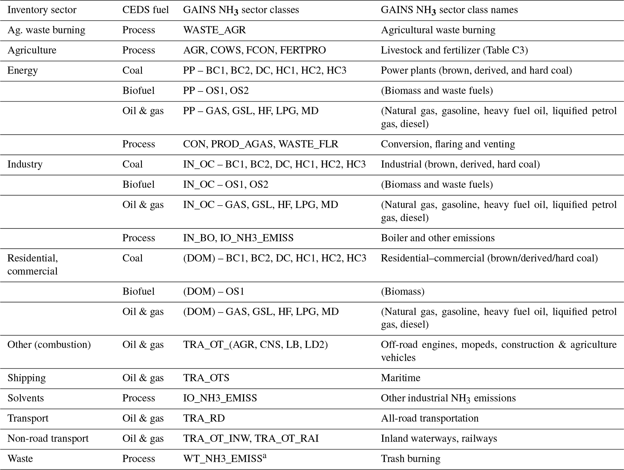
Table 1 Sectoral mapping and choice of scaling method for each inventory sector.

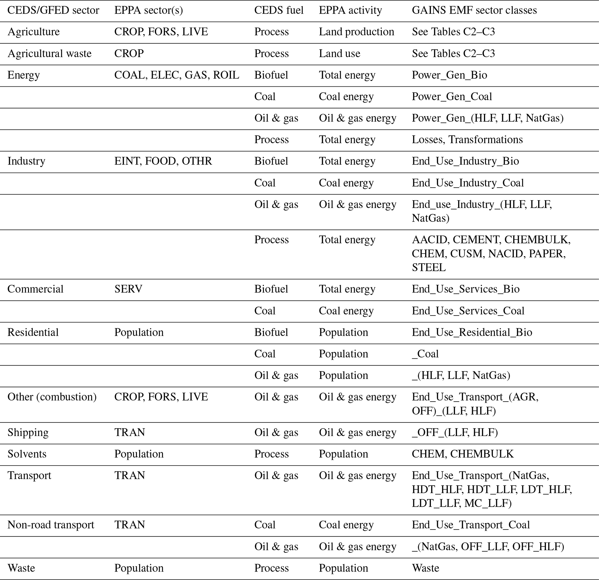
See online repository for full GAINS sector and fuel linkages. The CEDS fuel definitions are given in Table S1 of McDuffie et al. (2020a), with bioenergy separated between solid (“Biofuel”) and liquid fuels (“Oil & gas”). The CEDS/GAINS fuel type discrepancies were recalibrated based on the percent of CEDS fuel emissions covered by GAINS. Residential, Solvents, and Waste sectors were scaled by EPPA population projections, given the lack of sufficient corollary sectors in EPPA. Land production combines land use from EPPA (in area units) with production-per-area trends from corollary FAO (2018) scenarios. GAINS EMF sectors are given in Table S3 of Rafaj et al. (2021) and https://gains.iiasa.ac.at/models/index.html (last access: 5 October 2022).

First, we calculate emissions intensity trends for each GAINS sector by dividing the emissions time series by activity time series. Historical data are available for 2000, 2005, 2010, and 2015 – with projections for the CLE (2020, 2030, 2050) and MFR scenarios (2030, 2050). For missing activity data points, we conduct annual linear interpolation (and/or extension) for sectors with at least two values, or leave emissions intensities constant for sectors with one or no values. For trend extensions that reach zero before 2050, we assume values of zero thereafter. For the GAINS waste sectors – where only emissions (not activities) were given – we assume constant emissions intensities for CLE, and follow a recent GAINS paper on MFR's elimination of open burning (Gomez Sanabria et al., 2022) to apply region-specific trends to zero by 2050 for MFR (based on MFR/CLE emissions ratios). The NH₃ waste trends are matched to NO_x due to large data gaps.

For other NH₃ sectors, we employ a conservative approach towards estimating intensity reductions outside of the GAINS G20 regions. For MFR, we assume that the non-G20 regions follow the MFR intensity trend of their corollary G20 regions (Table C4) – but with constant intensities in CLE (only following the corollary if its intensity is constant or increasing). For agriculture sectors (where intensity could rise or fall due to shifting land use or dietary patterns), we also incorporate more granular sector trends from the FAO's 2050 scenarios of “Business as Usual” (CLE-like) and “Toward Sustainability” (MFR-like), which directly inform the GAINS database as well (FAO, 2018). The resulting intensity trend I combines the GAINS trend (GI) with FAO's trend for sector i relative to total production (F_r,t):

$$\begin{array}{}\text{(3)}& I_{f,i,j,r,t}={\mathrm{GI}}_{f,i,j,r,t}\times {\displaystyle \frac{F_{i,r,t}}{F_{r,t}}}.\end{array}$$

This adjustment allows for the potential of a region's overall agricultural intensity to change based on shifts in the relative share of the emitting sectors within agriculture (such as livestock categories, milk production, or fertilizer tonnage). Associated FAO sectoral and regional mappings are provided in Tables C3–C4.

Next, we prepare the GAINS sectors' emissions intensity trends for integration with EPPA activity trends. First, we scale the trends to a relative value of 1 in EPPA's base-year of 2014, using linear interpolation for the GAINS values of 5 years. To determine emissions intensity trends by CEDS sector–fuel combination (e.g., Industrial emissions from the “total-coal” fuel), we aggregate the more granular GAINS trends based on the proportion of the sector–fuel's emissions from that GAINS sector – adjusting to the proportion of emissions covered by GAINS in cases where not all the CEDS sector–fuel combinations had a GAINS equivalent. We repeat the process to aggregate from GAINS to EPPA regions.

2.4 Implemented scenarios

To illustrate an application of TAPS, we first select three scenarios from EPPA7 to represent variations in climate policy ambition (Table 2), based on Paltsev et al. (2021). The “Paris Forever” scenario assumes the completion of nationally determined contributions (NDCs) from the Paris Agreement (as of March 2021 with more recent adjustments for COVID-19), but no future climate policies beyond those near-term targets. The other two scenarios extend this NDC baseline to the Paris Agreement's long-term temperature goals, using a global emissions cap and price starting in 2030 to provide a 50 % chance of limiting warming to 2 ^∘C or 1.5 ^∘C above pre-industrial levels. (Temperature estimates come from ensemble linkages of the MIT Earth System Model (Sokolov et al., 2018), or MESM, to EPPA's economic results). The 1.5 ^∘C scenario features an almost 50 % reduction in GHG emissions from 2025 to 2030, a highly ambitious projection. As such, these scenarios span a range from current pledges to a much more stringent set of future climate policies.

Table 2 EPPA7 scenarios analyzed, with selected SSP comparisons.

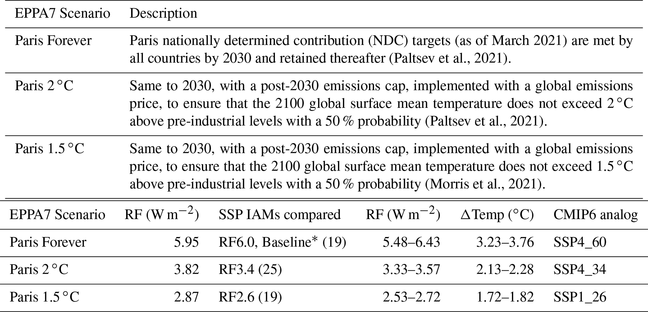
Radiative forcing (RF) and IAM-based temperature change are global mean values for 2100, relative to pre-industrial levels of 1861–1880 in EPPA (Morris et al., 2021) and 1850–1900 for the SSPs (Riahi et al., 2020). The CMIP6 analog shows the SSP and RF combination that is most similar to each EPPA scenario. ^* IAM scenarios were not included if the RF difference from EPPA was greater than 0.5 W m⁻².

This range is reflected in the corresponding FAO (2018) scenarios used for agricultural production scaling: “Business as Usual” for “Paris Forever” and “Towards Sustainability” for the 2 and 1.5 ^∘C scenarios. In Table 2, we also compare results from each EPPA scenario to CMIP6 scenarios and additional IAM runs from SSPs that have similar radiative forcing (RF) and other assumptions (Feng et al., 2020). While the “SSP5-3.4-Overshoot” scenario does fall in the EPPA forcing ranges, it assumes business-as-usual emissions in the near-term and plentiful negative emissions technologies in the long-term, in contrast to the EPPA scenarios' near-term NDCs and lack of negative emissions.

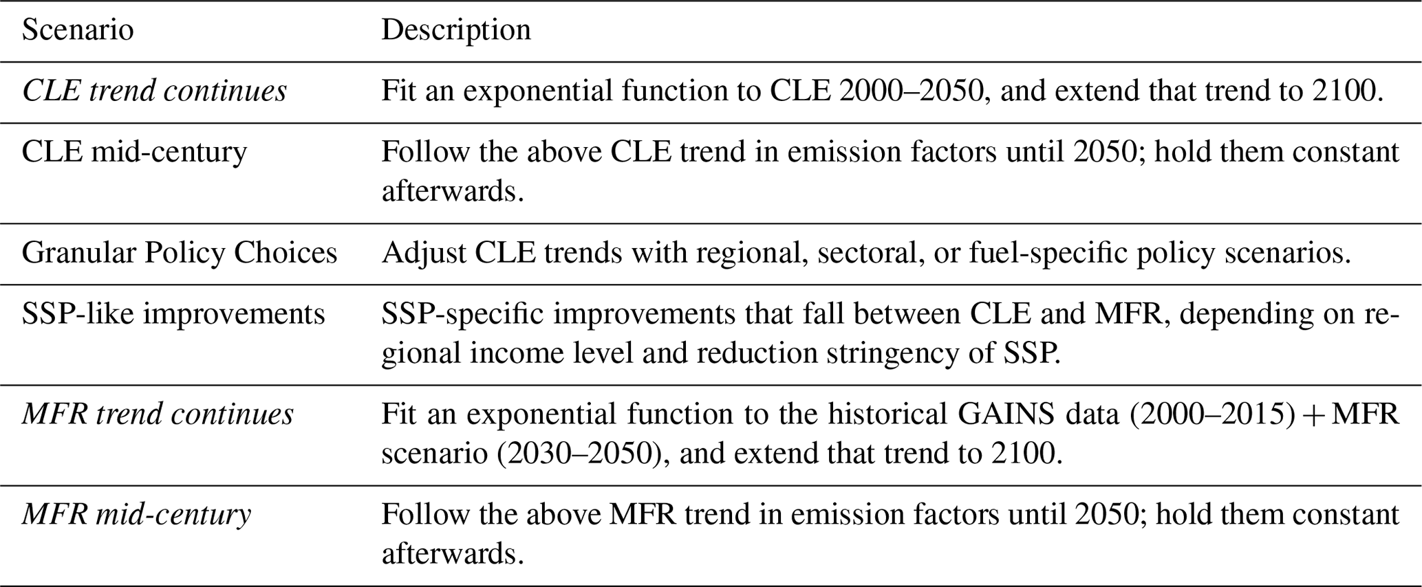
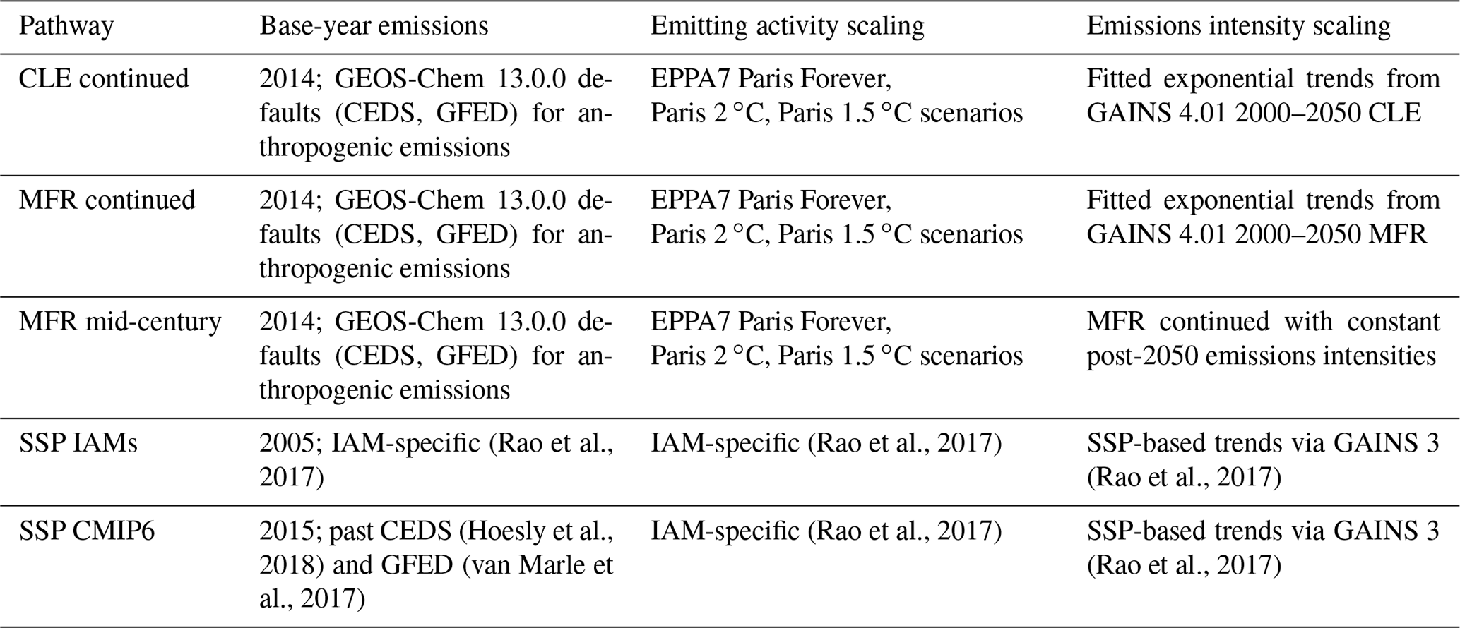
Turning to pollution control, we use this initial implementation to show the range of outcomes between GAINS CLE and MFR scenarios, based on version 6b of project ECLIPSE (Evaluating the Climate and Air Quality Impacts of Short-Lived Pollutants) as presented by Stohl (2015) and online (IIASA ECLIPSE V6, 2021). After aggregating the GAINS emissions intensity trends to inventory sectors and EPPA regions (Sect. 2.3), we perform exponential fits for all non-constant intensity pathways to enable simpler scenario tuning and harmonization with EPPA's trends out to 2100. Our approach helps assess the potential of future innovation over the next 8 decades beyond today's best available technologies, in the case of MFR. We also incorporate the possibility of no such innovation, showing an “MFR Mid-century” scenario that limits pollution control to the 2050 levels in GAINS. (Other studies could explore other scenarios based on the research question; we describe examples in the discussion and Table 3.) Exponentials are designed to pass through base-year values of 1 and MFR waste values of zero for 2050 onward (using uncertainty weightings of 0.01 via Python's scipy curve fitting's sigma parameter). Given the MFR scenario's definition as the maximum feasible pollution reduction, anomalous cases with higher intensities than the corresponding CLE pathway are fixed to CLE levels.

The resulting trends in emissions intensity are reported in the online repository (before and after exponential fits), with ∼ 5500 trajectories from the 2 GAINS scenarios, 7 pollutants, 18 EPPA regions, and ∼ 20 CEDS sector–fuel combinations. The fit data include reported r² values that range from strong (particularly for areas with full data sets such as Western Europe) to weaker in cases with incomplete or abrupt changes in emissions intensities. The trends are highly sector- and region-specific, ranging from sharp decreases (such as 10–100× drops in some transportation cases) to occasional increases (sometimes due to projected fuel switching within the GAINS activities that had been aggregated to the 56 EMF sectors). Increased intensities include CO emissions from steel in Brazil, Africa, and Eastern Europe, as well as SO₂ coal emissions from residential (Eastern Europe) and end-use industry (Western Europe). Finally, we combine the intensity trends with the linked base-year inventories and revised activity scaling (Eq. 1). Results are presented below and in the online repository, including outputs of all individual emissions trends as well as summary sheets of inventory value, activity scaling, and intensity scaling at notable time points (2030, 2050, 2100) for quicker comparisons.

Table 3 Example emissions intensity trends, based on GAINS scenarios of current legislation (CLE) and maximum feasible reduction (MFR). Results from italicized scenarios are shown in Figs. 2–6.

For more detailed information on SSP scenarios, see Tables 1–2 of the Supporting Information in Rao et al. (2017).

3 Results

3.1 Example scenario and SSP comparison

We illustrate an application of TAPS by providing the results for total air pollutant emission trends (Fig. 2), sectoral breakdowns (Figs. 3–4) and regional breakdowns (Figs. 5–6). We also compare this implementation to corresponding SSP, IAM, and CMIP6 scenarios (summarized in Table 4), which serve a different research purpose than TAPS (and thus are not expected to match) but can act as a useful reference point. For Fig. 2, we show the full range of SSP–IAM combinations that have a similar radiative forcing to each of the three EPPA-MESM climate scenarios in Table 2. Though the SSPs and EPPA-MESM have slightly different temperature change estimates for a given forcing level, this process represents the closest comparison available between the two data sets. We facilitate this comparison by removing the SSP sectors that are not part of our scaling (aviation and open burning beyond agricultural waste), based on their emissions proportion in the best-fitting CMIP6 scenario (since sectoral non-CMIP6 IAM emissions are not available). This estimate may lead to slight visual differences in SSP data between Figs. 2 (IAM) and 3–6 (CMIP6), but acts as a reasonable first-order comparison with the TAPS scaling.

Figure 2 Global air pollutant emissions trends within the range of GAINS-based scenarios of current legislation (CLE Continued Trend) and maximum feasible reduction (MFR Mid-century; MFR Continued Trend) in Table 3 (top to bottom in purple), as compared to the range of SSP IAM corollaries in Table 2 (blue). The IAM estimates are subtracted by sectors not scaled by TAPS (aviation and open burning beyond agricultural waste), based on the proportion of their emissions in the best-fitting CMIP6 scenario (since sectoral IAM emissions are not available). Quantities of NO_x are in Tg NO₂; quantities of BC, OC, and NMVOC are in Tg C.

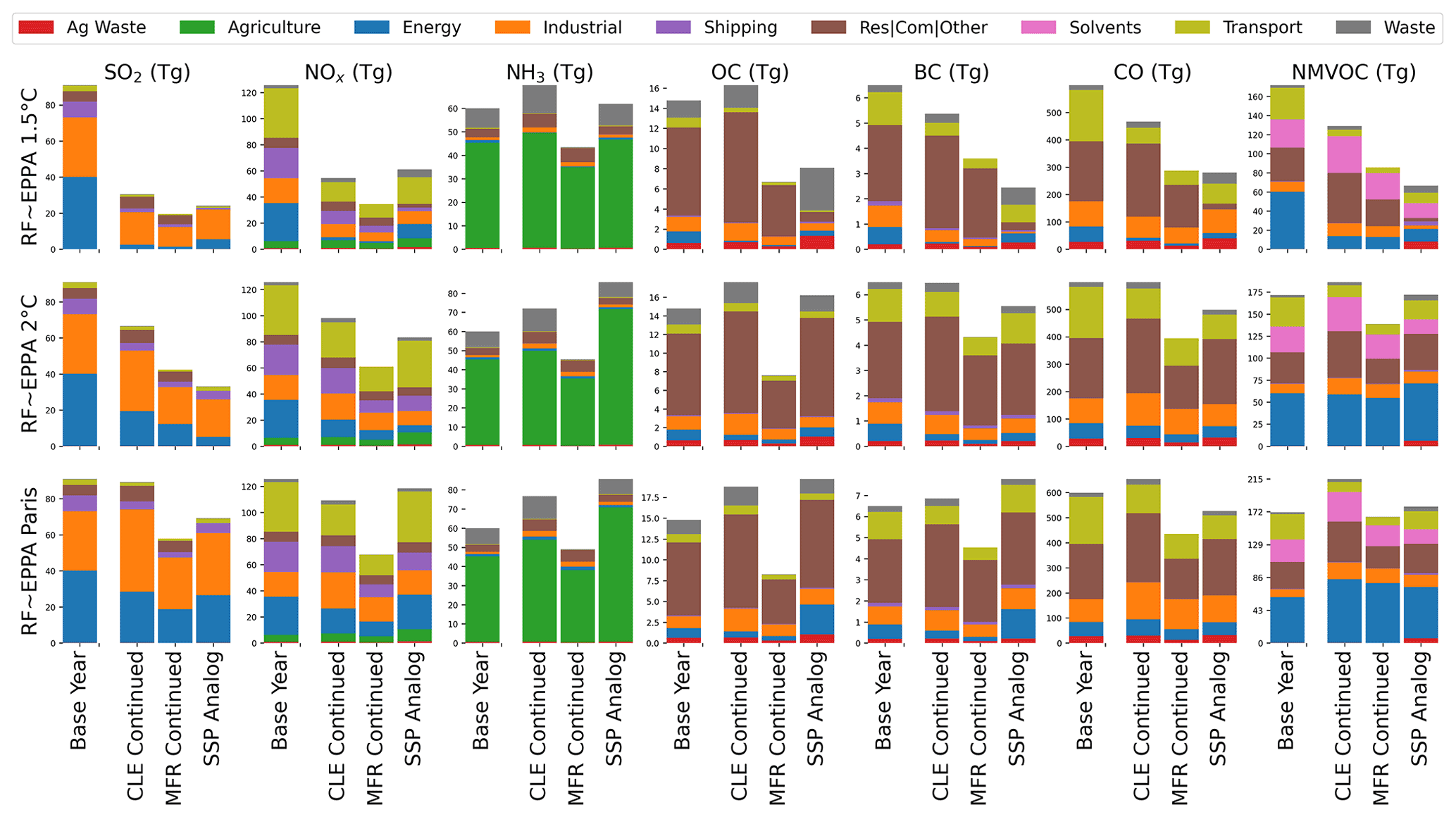
Figure 3 Sectoral emissions of air pollutants in 2050 under the GAINS-based scenarios of current legislation (CLE) and maximum feasible reduction (MFR) continued – along with the 2014 emissions inventories and corresponding CMIP6 scenarios of SSP1-2.6, SSP4-3.4, and SSP4-6.0 (respectively) for EPPA's 1.5, 2 ^∘C, and Paris Forever scenarios (see Table 2). The 11 CEDS_GBD-MAPS sectors (McDuffie et al., 2020a) are condensed to the 8 in the earlier version used by the SSPs (Hoesly et al., 2018), including the aggregation of residential, commercial, and other combustion (“Res|Com|Other”), plus agricultural waste burning (“Ag Waste”) from GFED. Quantities of NO_x are in Tg NO₂; BC, OC, and NMVOC are in Tg C.

Figure 4 Same as Fig. 3 but for 2100, and including the MFR Mid-century scenario in Table 3.

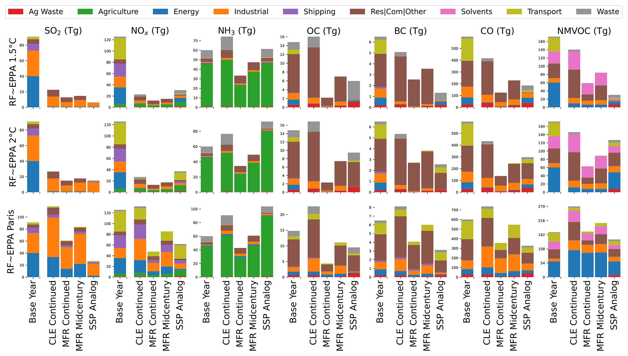
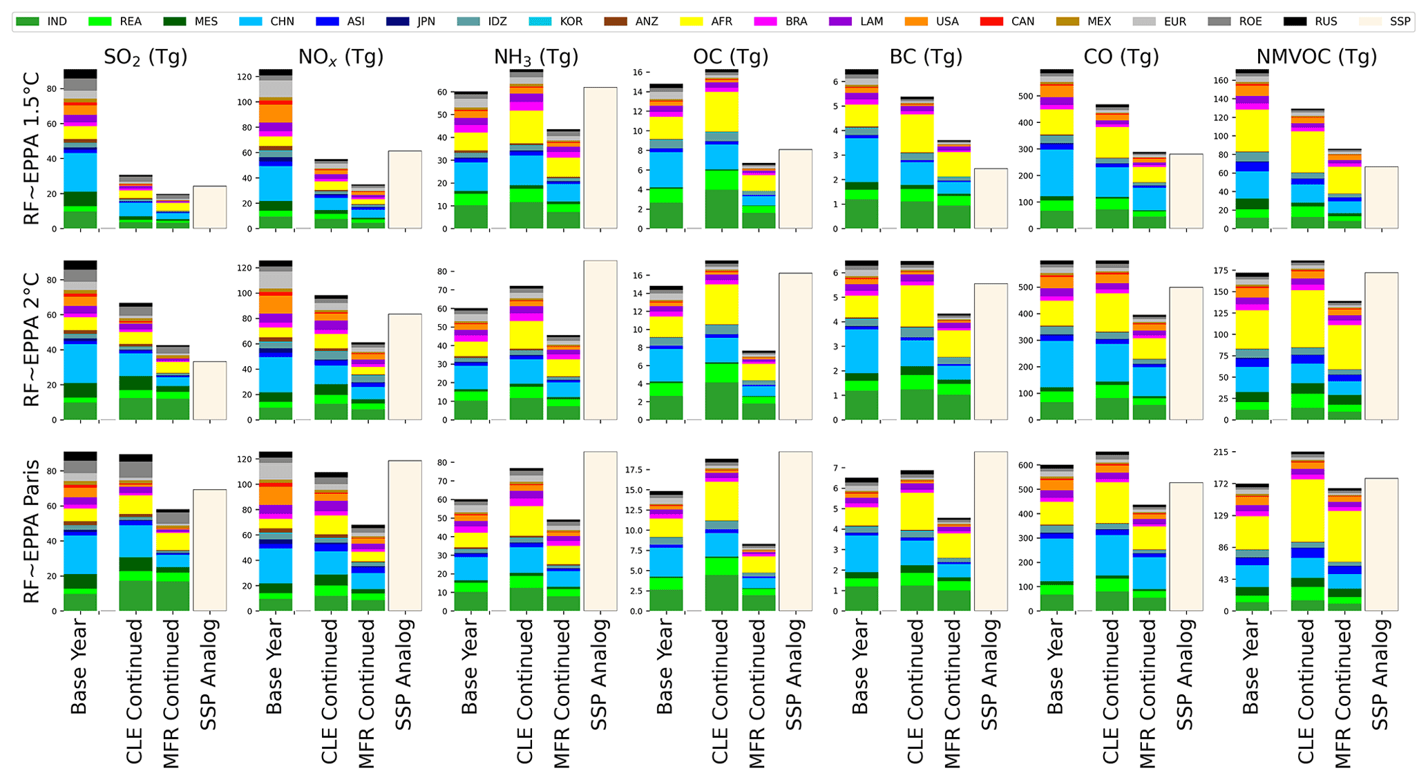
Figure 5 Regional emissions of air pollutants in 2050 under the GAINS-based scenarios of current legislation (CLE) and maximum feasible reduction (MFR) continued – as compared to the 2014 emissions inventories and corresponding CMIP6 scenarios of SSP1-2.6, SSP4-3.4, and SSP4-6.0 (respectively) for EPPA's 1.5, 2 ^∘C, and Paris Forever scenarios (as in Table 2). See Table B1 for EPPA region abbreviations. The SSP values are shown as global totals due to regional definition discrepancies. Quantities of NO_x are in Tg NO₂; BC, OC, and NMVOC are in Tg C.

Figure 6 Same as Fig. 5 but for 2100, and including the MFR Mid-century scenario in Table 3.

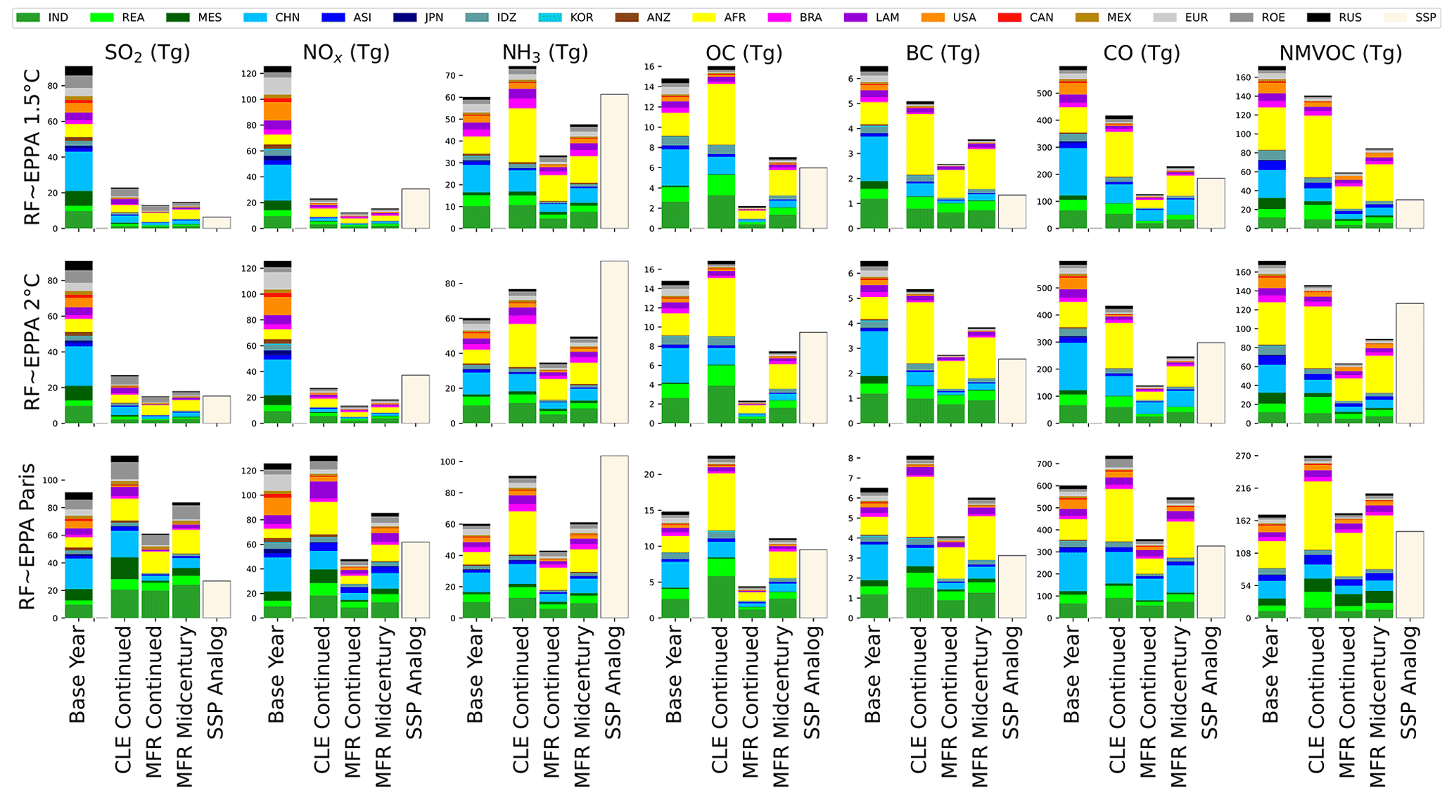
Table 4 Summary of pathways presented.

SSP corollaries from the full range of IAMs are shown in Fig. 2, while sectoral data (Figs. 3–4) are only available from the CMIP6 subset. For more detailed information on IAM model inputs, see Sect. 2.2 of the Supporting Information in Rao et al. (2017).

When comparing initial emissions, IAM inventories differ both in base year (2005 versus EPPA7's 2014) and emissions values (Fig. 2) – given their variety of sources from the Emissions Database for Global Atmospheric Research (EDGAR) to GAINS to the Radiative Concentration Pathway (RCP) or even older IPCC inventories (Rao et al., 2017). Even after the inventories have been harmonized in the CMIP6 scenarios (Gidden et al., 2019), their use of an earlier CEDS version (Hoesly et al., 2018) leads to differences such as a base-year OC value that is 30 % higher than the updated CEDS value (McDuffie et al., 2020a). The NMVOC inventories of emissions inside the scope of CEDS are also much lower in the IAMs, especially from the Integrated Model to Assess the Global Environment (IMAGE) model and coupling of the Regional Model of Investment and Development with the Model of Agricultural Production and its Impact on the Environment (REMIND-MAgPIE) models (Riahi et al., 2020).

In the TAPS example policy scenarios, emissions often trend much higher if activity and intensity reductions are limited to current legislation. This result differs from the SSPs, which include actions beyond current legislation to answer different research questions (Rao et al., 2017). While recent studies support cases of increased emissions under current legislation (Rafaj et al., 2021), they focus on trends to mid-century. Here, many of the increases are strongest in the late century – implying that any continued improvements in the GAINS-based intensity trends are offset by further increases in activity. This contrast is strongest in industrial “process” emissions sources, where EPPA's sharp increases in activity overpower the slight decreases in emissions intensity. While the modeled trends to 2100 are shown for context, the sectoral and regional plots also focus on 2050 as the last year with official GAINS scenario data. We next summarize projections for each pollutant category in turn.

3.2 Example scenario results by pollutant

In the case of increasing SO₂ under EPPA's “Paris Forever” and GAINS' CLE scenarios, continued coal use without desulfurization and/or carbon capture is the primary factor – especially in regions with fewer current pollution controls such as Africa, South Asia, and Eastern Europe. These regions also generally have NDCs (as of March 2021) that fail to phase down coal, according to Table 3 of Paltsev et al. (2021). By 2100, the doubling of industrial and residential sector emissions outpaces the decreases in energy and transport sectors. Industrial increases are driven by increased activities (4- to 10-fold by 2100 in those regions) with few intensity improvements, while residential increases are driven by a sharp increase in GAINS-based emissions intensity from coal use in Eastern Europe. The GAINS MFR intensities are much lower given the additional pollution controls, halving the industrial emissions compared to CLE and leading to a 3-fold drop in energy sector emissions by 2100. Still, the increased coal activities of “Paris Forever” (especially in developing areas' non-energy sectors) prevent emissions from decreasing globally, as in Rafaj et al. (2021). More ambitious climate policy scenarios include rapid declines in coal energy use – leading to declining SO₂ emissions, even if the intensities of the few remaining emissions sources (mostly industrial and residential) are nonzero.

The CO and NMVOC emissions show similar trends. In the case of CO under CLE and “Paris Forever”, industrial processes increase in activity (up to 10-fold in India by 2100) as well as intensity for certain regions (4-fold in Africa and 5-fold in Eastern Europe). Pollution controls in MFR reduce these increases, while causing major declines in most other sectors (including residential, unlike with SO₂). The NMVOC emissions follow these general patterns, with greater influence from energy process sources that have fewer control options in GAINS and more temporal variation from EPPA trends. The CLE emissions intensities are relatively flat for energy, industrial, and solvent process sources (with some increases in Brazil and much of Asia), leading to greater emissions under the “Paris Forever” scenario. Further climate policy leads to further declines in energy, transport, and industrial coal, while further pollution policy (in MFR) is more impactful for solvents, residential, and industrial process sources.

Long-term NO_x emissions also increase under less ambitious policies, given the limits of projected intensity improvements in GAINS CLE. In this pathway, increased activities in EPPA lead to increased agriculture and a doubling of industry emissions by 2100 (including a 10-fold increase in India's oil and gas fuel), offsetting initial declines from GAINS intensities and overall reductions in other sectors like energy and transport. The GAINS MFR case gives further intensity reductions, flattening industrial emissions and transitioning energy and transport to near-zero. The result is a near-halving of overall emissions by mid-century, though rising activities cause rising emissions after 2050 if intensities are held at 2050 levels under the “MFR Mid-century” scenario (as with SO₂ and CO). With further climate policy in the 2 and 1.5 ^∘C scenarios, oil and gas use in EPPA is projected to reach near-zero by late-century as well, leading to lower emissions than most of the IAMs (which may assume less steep energy declines due to their greater reliance on negative emissions).

Black carbon (BC) and OC are driven more by residential emissions, which have limited intensity improvements in CLE but much stronger pollution controls in MFR. The BC emissions are generally higher than their SSP counterparts, as increased activities overpower intensity improvements for residential, commercial, industrial, and waste sectors. Moving to MFR leads to decreases in all sectors except for commercial, while moving to a 2 ^∘C climate scenario reduces energy and industry but not the others. Pollution control actions have an even greater effect for OC. In “MFR Continued” under “Paris Forever”, OC residential and industrial emissions drop 8-fold and 7-fold, respectively, from 2014 to 2100, compared to 2-fold drops in “MFR Mid-century” and visible increases in both sectors under CLE. Across the OC scenarios, adding pollution control ambition leads to more emissions reductions than increasing the climate policy ambition.

Ammonia (NH₃) also shows the pronounced effect of pollution control outside of climate policy. In CLE cases, increased agricultural production globally combines with a near-doubled intensity in Africa (by 2100) to offset slight efficiencies elsewhere. When the FAO scenario is changed from “Business as Usual” (CLE-like) to “Toward Sustainability” (MFR-like), the spread of activities is much less emissions-intensive (near-constant in Africa, Eastern Europe, and the Middle East; substantially decreasing elsewhere), and relatively flat land use trends allow for declines in overall emissions. Non-agricultural NH₃ emissions play a smaller role but follow similar patterns, with increased emissions under the limited existing policies and further reductions (such as in waste) under more ambitious policies.

4 Discussion

Several factors can help explain the different projection scenarios of TAPS and the SSPs. Most importantly, the two scenario sets serve different research goals, as the SSPs specify future pollution controls in line with each socioeconomic pathway (versus our broader range of outcomes). In practice, this leads to SSP emission factors that may trend much lower than CLE, according to Tables 1–2 and Fig. 1–1 of the Supporting Information in Rao et al. (2017). The resulting scenarios often have lower emissions than our “CLE Continued Trend”, as well as other studies of GAINS CLE with the CMIP6 IAMs (Rafaj et al., 2021). The relevance of each scenario set will depend on the question at hand, and whether the underlying research question that users seek to address can be answered by applying a specific socioeconomic pathway, or would benefit from a framework such as TAPS in which assumptions about air pollution are decoupled.

Other discrepancies may result from updated model data. Sectoral scaling choices differ between IAMs, as described in Sect. 2.2 of the Supporting Information in Rao et al. (2017). One example is the much higher value for OC waste emissions in SSP1-2.6 versus this study (Fig. 3), which comes from a constant-emissions extension of the higher inventory value from the associated IMAGE model (Riahi et al., 2020). Another difference is the climate policy landscape that has changed between the SSP modeling process (mid-2010s) and the 2021 EPPA scenarios. While the latter may incorporate newer NDC pledges, the SSP IAMs sometimes assumed greater clean energy access and therefore lower biofuel-related BC emissions, for example (Riahi et al., 2020).

There are also differences between emissions intensity projections in GAINS 3/ECLIPSE v5a (used by SSPs) and GAINS 4/ECLIPSE v6b (used here), as the latter includes newer regulatory or technological levers. This is certainly the case for the waste sector, with intensity trends changing from near-constant in GAINS 3 to a net-zero MFR endpoint (elimination of open burning of municipal waste) in GAINS 4 (Gomez Sanabria et al., 2022). More granular regions and sectors, such as the refinement of residential cooking and heating (GAINS Developer Team, 2021a), could also affect the pathways where those sectors play major roles (like for BC and OC). In addition, the updates reflect the effects of some recent policies, such as the sharp declines of SO₂ in China (Zheng et al., 2018).

It is also worth noting the differing structures of each integrated data set in TAPS, particularly with respect to the sectors and regions of CEDS, GFED, EPPA, GAINS, and FAO. The lack of direct EPPA matches for the CEDS sectors of “Residential”, “Solvents”, and “Waste” necessitates a scaling by population that limits the sectors' range of outcomes. We also make approximations for solid biofuel categories of CEDS, scaling by EPPA's total sectoral energy, given the lack of a closer fit. Finally, the regional estimates of NH₃ trends beyond the available G20 data (chosen as constant or G20-like intensity paths for each GAINS sector) could be low or high, depending on the realities in those areas. Future work could refine these assumptions as improvements become available.

Further application of TAPS could explore other emissions intensity scenarios to inform different research questions (Table 3). This example application demonstrates the range of outcomes between the bounds of a “CLE Continued Trend” and “MFR Continued Trend” (as well as the more conservative “MFR Mid-century” variation), embodied by the fitted exponentials described above. For other applications, a “CLE Mid-century” case (with emission factors held at the final GAINS data point in 2050) could parallel the “Paris Forever” focus on short-term greenhouse gas policy, while the SSP-like scenarios could be used for more direct comparisons with their income-based pathways. Finally, additional scenario elements such as land use, diet, and active mobility could be incorporated as in recent works – particularly since improving such elements may lead to comparable or even greater health benefits than the pollution-specific policy levers explored here (Amann et al., 2020; Hamilton et al., 2021).

Such scenarios need not be limited to emissions intensity. With the regional, sectoral, and fuel-based EPPA outputs given in the data and code availability, users can readily explore the effects of more granular climate policies applied at those levels. Activity trends could be adjusted to study the effects of sector-specific policies on agricultural land use, fuel-specific policies on coal combustion levels, or region-specific policies that capture individual NDC updates, for example. Given the tool's relatively quick runtime, uncertainty analyses could explore larger ensembles of policy or other inputs to efficiently explore first-order outcome ranges, following the approach of recent EPPA studies on socioeconomic (Morris et al., 2022) and climate forcing trends (Morris et al., 2021).

5 Conclusions

TAPS provides a flexible and comprehensive model for assessing climate and pollution pathways, integrating recent standard emissions inventories, long-term activity scaling, and scenario-specific emissions intensities. Results from its application to selected scenarios show lower near-term emissions than the SSPs in many cases, both from NDCs' greater climate policy ambition as well as recent pollution reduction actions now captured in GAINS. Less ambitious pathways show increased emissions in the long-term – particularly for the industrial and agricultural processes that have fewer existing controls. These increases are especially pronounced in developing regions where sharply growing activities are combined with fewer planned pollution policies. However, more ambitious climate and pollution policies can curb those increases substantially – from the SO₂ and NO_x reductions driven by fuel switching to the NH₃ reductions from land use decisions and OC reductions from pollution controls.

Future applications could explore other scenarios by adjusting a range of climate or pollution policy inputs. Assessing other climate or activity scenarios could compare the health impacts of near-term fuel switching versus long-term negative emissions. Additional emissions intensity trends could add the aforementioned elements of land use, diet, or specific innovations beyond today's technological control options. All these scenarios can be applied to specific regions, sectors, or fuels in the framework to explore more granular policies or target short-term actions with high-impact benefits.

Future tool development and linkages could consider other emissions sources – such as aviation, open burning, or wildfires – to explore the futures of additional activities that may be underestimated (Pan et al., 2020) or not fully covered by the default inventories used here. Integration with other modeling tools could examine key inter-pollutant or pollutant-climate feedbacks, such as the increased NH₃ emissions rates in a warming world (Yang et al., 2021). External coupling to other ensemble results could address important but out-of-scope elements such as meteorological uncertainty, given its importance in past studies that compared natural variability with other sources of uncertainty in health impacts analysis of air pollution (Pienkosz et al., 2019; Saari et al., 2019).

Finally, additional research with air quality and impact models can assess the health, economic, and ecological effects of TAPS emissions scenarios as well as their implications for decision-making. Quantified impacts could include a range of mortality and morbidity endpoints to reflect recent epidemiological research (Danesh Yazdi et al., 2019), as well as other vulnerabilities (such as crops, biodiversity, and forestry) or analyses of equity, uncertainty, and sensitivity for key parameters (Hess et al., 2020). Using a combined assessment of climate and pollution policies could help to reduce the silos that have traditionally hindered the consideration of climate–health linkages in decision-making (Workman et al., 2018). Integrated impact metrics (whether through the weighting of multi-criteria decision analysis or the monetization of benefit-cost analysis) could also inform policy conversations. Ultimately, the TAPS framework could enable more flexible, efficient, and extensive scenario study of policies that affect climate change and health futures.

Appendix A: CEDS reference data

Table A1 Percentage of base-year (2014) CEDS emissions from different fuel consumption versus process sources (broken down by sector, aggregated globally).

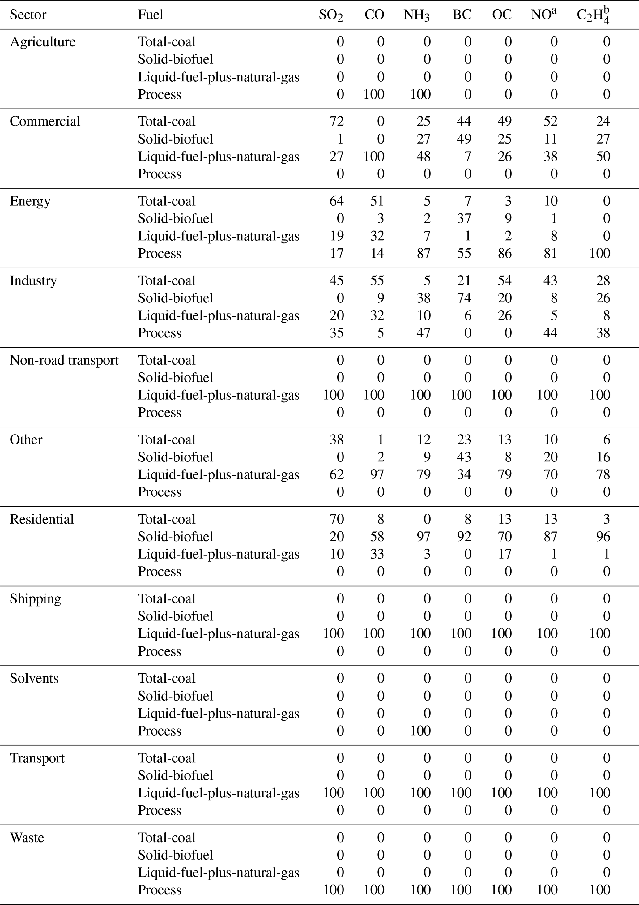
^a CEDS reports NO_x as NO and NMVOC as speciated compounds; ^b C₂H₄ is shown as an example NMVOC species. Other NMVOC species may show differences, such as more “process” emissions from solvents. Global aggregate proportions are shown here for context; full regional and speciated values are available at our online repository. The CEDS fuel definitions are given in Table S1 of McDuffie et al. (2020a), with bioenergy separated between solid and liquid fuels.

Appendix B: EPPA7 reference definitions

Table B1 EPPA7 regions and sectors, as described in Paltsev et al. (2021).

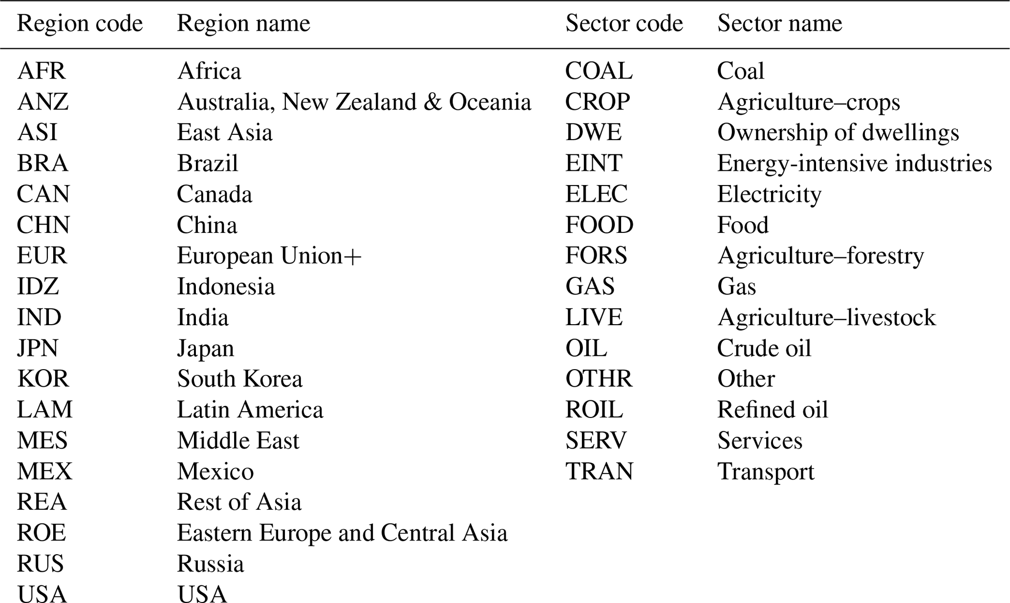
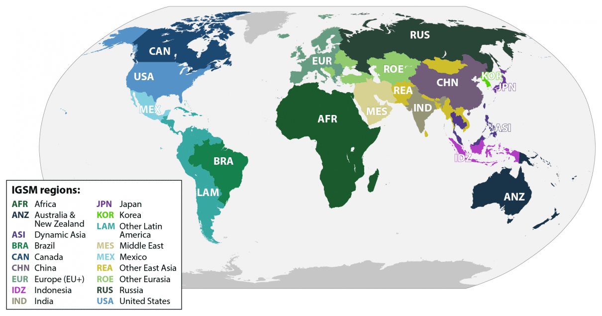
Figure B1 Map of EPPA7 regions of the world, from Paltsev et al. (2021) and online documentation of its Integrated Global System Modeling (IGSM) framework (https://globalchange.mit.edu/research/research-tools/eppa, last access: 5 October 2022) with reproduction rights granted.

Appendix C: Mapping from GAINS model

Table C1 Mapping from GAINS EMF (based on IMAGE) to EPPA7 regions.

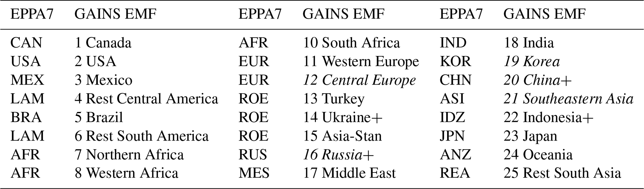
IMAGE regions are given in Fig. S7.1 of Klimont et al. (2017) and compared to Fig. 2. Regions in italic differ slightly from EPPA definitions.

Table C2 Mapping from GAINS NH₃ to CEDS/GFED inventory sectors and fuels.

See full table (with a row for each of the 198 GAINS NH₃ sectors) in the online repository. CEDS fuel definitions are given in Table S1 of McDuffie et al. (2020a) – with bioenergy separated between solid (“Biofuel”) and liquid fuels (“Oil & gas”). Comparisons are based on Table S3 in Rafaj et al. (2021), with sectoral abbreviations described further in GAINS Online. ^a Since NH₃ “Waste” data were only available for two countries, emissions intensity trends follow NO_x “Waste” trends based on Gomez Sanabria et al. (2022).

Table C3 Mapping from GAINS agricultural sectors to FAO activities.

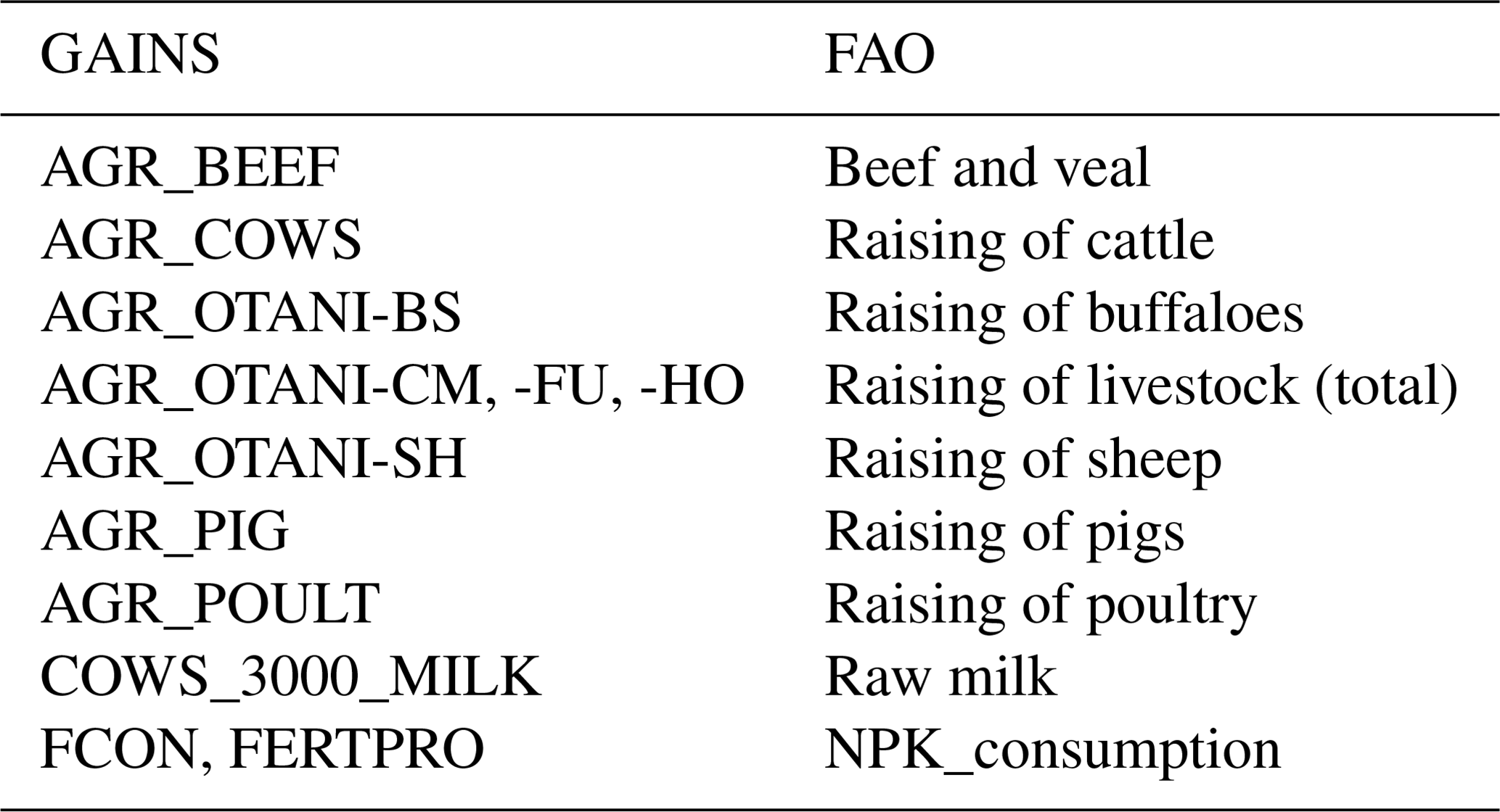
Based on GAINS sector abbreviations at https://gains.iiasa.ac.at/models/index.html (last access: 5 October 2022) and FAO sectors in regional aggregate data.

Table C4 Mapping from NH₃ data sources to EPPA7 regions.

Full GAINS data were only provided for G20 countries. Countries that approximate other regions are shown in bold, while corollaries that represent a part of their EPPA regions (or vice versa) are in italic. FAO regions are shown in Fig. 1.2 of FAO (2018). ^a Countries with subnational regions in GAINS were aggregated based on their proportional emissions. ^b Scaling for EPPA regions not well-captured by the GAINS G20 coverage is described in Sect. 2.3.

Appendix D: IPCC sectoral references

Table D1 IPCC sectoral definitions for EPPA scaling of sectors from the chosen emissions inventories. N/A sectors are not included in CEDS_GBD-MAPS.

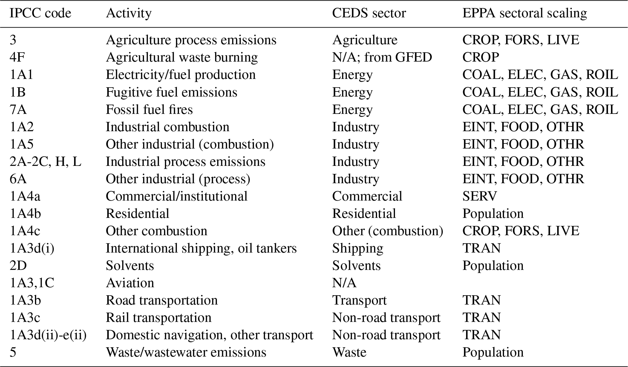
Inventory versions include CEDS_GBD-MAPS (McDuffie et al., 2020a) for most anthropogenic emissions, as well as GFED4.1s (van der Werf et al., 2017) for biomass burning. Since only agricultural waste burning is included in EPPA through GTAP/EDGAR, other sources of burning emissions are not scaled by EPPA outputs. Aviation was not scaled in this work due to its exclusion from both CEDS_GBD-MAPS and GAINS. “Other combustion” includes sources from agriculture, forestry, and fishing. Sectoral scaling from EPPA largely reflects the distribution of activities in GTAP10/EDGAR5.0 sectors (Chepeliev, 2020), which are then mapped to representative EPPA7 sectors.