Implementing the Water, HEat and Transport model in GEOframe (WHETGEO-1D v.1.0): algorithms, informatics, design patterns, open science features, and 1D deployment

This paper presents WHETGEO and its 1D deployment: a new physically based model simulating the water and energy budgets in a soil column. The purpose of this contribution is twofold. First, we discuss the mathematical and numerical issues involved in solving the Richardson–Richards equation, conventionally known as the Richards equation, and the heat equation in heterogeneous soils. In particular, for the Richardson–Richards equation (R²) we take advantage of the nested Newton–Casulli–Zanolli (NCZ) algorithm that ensures the convergence of the numerical solution in any condition. Second, starting from numerical and modelling needs, we present the design of software that is intended to be the first building block of a new customizable land-surface model that is integrated with process-based hydrology. WHETGEO is developed as an open-source code, adopting the object-oriented paradigm and a generic programming approach in order to improve its usability and expandability. WHETGEO is fully integrated into the GEOframe/OMS3 system, allowing the use of the many ancillary tools it provides. Finally, the paper presents the 1D deployment of WHETGEO, WHETGEO-1D, which has been tested against the available analytical solutions presented in the Appendix.

1 Introduction

The Earth's critical zone (CZ) is defined as the heterogeneous near-surface environment in which complex interactions involving rock, soil, water, air, and living organisms regulate the natural habitat and determine the availability of life-sustaining resources (National Research Council, 2001). Clear interest in studying the CZ is spurred on by ever-increasing pressure due to growth in the human population and climatic changes. Central to simulating the processes in the CZ is the study of soil moisture dynamics (Clark et al., 2015a; Tubini et al., 2021b). In the following we suggest that studying the CZ requires tools that are not yet readily available to researchers; then we propose one of our own. These tools should be flexible enough to allow the quick embedding of advancements in science.

1.1 Setting up the water budget

It is generally accepted in the field that the motion of water in soil is regulated by a Darcian–Stokesian flow, meaning that any force is immediately dissipated and water under a gradient of generalized forces acquires a velocity (the Darcy velocity) which is linearly proportional to the gradient of the generalized force. This law is known as the Darcy–Buckingham law and reads

$$\begin{array}{}\text{(1)}& \mathit{J}=K\left(\mathit{\theta }\right)\mathbf{\nabla }\left(\mathit{\psi }+z\right),\end{array}$$

where the forces acting are gravity (z; L) and the matric potential ψ [L] and where J [L T⁻¹] is the Darcian flux, K [L T⁻¹] is the hydraulic conductivity, θ [L³ L⁻³] is the dimensionless volumetric water content, ∇ [L⁻¹] is the gradient operator, and z [L] is the vertical coordinate positive-upward. The assumptions under which such a law is derived from Newton's law are presented in Whitaker (1986) and Di Nucci (2014). The hydraulic conductivity depends on soil type (texture and structure) and water content, while the thermodynamic forces must be understood as gradients of the chemical potential of water, which, in turn, can be split in matric potential, osmotic potential, and other potentials (Nobel, 1999, chap. 2). However, in Eq. (1) we consider only the action of the matric potential. On the basis of the law of motion in Eq. (1), the mass conservation reads

$$\begin{array}{}\text{(2)}& {\displaystyle \frac{\partial \mathit{\theta }}{\partial t}}=\mathrm{\nabla }\cdot \left(K\left(\mathit{\theta }\right)\mathbf{\nabla }\left(\mathit{\psi }+z\right)\right),\end{array}$$

where ∇⋅ [L⁻¹] is the divergence operator. Equation (2) is usually known as the Richards equation (Richards, 1931) but was previously formulated by Richardson (1922). Therefore, in the following we call it the R² equation to remind the reader of this double origin. There are very informative reviews that cover its general, historical, and numerical aspects, such as Paniconi and Putti (2015), Farthing and Ogden (2017), and Zha et al. (2019). Therefore, it is not deemed necessary to further summarize the matter here. The R² equation is a function of two variables, θ and ψ, and its resolution requires another relation between these two quantities. This relation is known as soil water retention curves (SWRCs), written in the plural because we have many SWRCs depending on soil characteristics. The reader may be aware that the R² is an exact description of unsaturated flow only if we assume that soil is a bundle of capillaries and that the largest capillaries drain first and are filled last (Mualem, 1976). In fact, in this case a relation can be obtained between the radius of the capillaries and the suction, which was fully derived (Kosugi, 1999). However, there are various reasons to take the capillary bundle concept as a rough approximation of natural soil. Some of the issues are enumerated below.

1. Firstly, pores in soils are not bundles of well-defined capillaries of a single diameter; in fact, they can have quite random structures, as revealed, for instance, by tomography (Yang et al., 2018).

2. Secondly, logic and pore scale simulations, as in Tomin and Lunati (2016), for example, indicate that fluids fill the cavities where they fall, and only eventually are they redistributed according to the microstructure of the soil; that is to say that fluids do not move instantaneously from the largest pores to the smallest ones.

3. A set of relatively large pores can, in certain conditions, preferentially drive the flow of water in a short timescale according to laminar viscous flow driven by gravity before any redistribution happens (Germann and Beven, 1981).

4. The role of living matter, such as bacteria, animals, fungi, vegetation, and roots, is usually eliminated from the hydrological picture, but it should have a relevant place (Benard et al., 2019).

In addition are the following points.

• 5.

  Capillary forces are not the only ones acting at the microscale (Lu, 2016). In fact, measured suction values are far below pressures that can be sustained by capillarity alone.

• 6.

  Temperature affects water viscosity; infiltration is faster at warm temperatures and slower at cold ones (Constantz and Murphy, 1991).

• 7.

  In high-latitude and high-elevation environments, soils may be subject to freezing and thawing processes which affect pore volume and water dynamics (Dall'Amico et al., 2011).

These facts certainly do not threaten the nature of mass conservation in Eq. (2). However, they can certainly alter the statistics which generate the closure equations, i.e. the SWRCs we currently use.

• Requirement I – without entering into further details, we can observe that the aforementioned issues have consequences that would require new software to include the possibility of adopting new parameterizations of SWRCs and hydraulic conductivity quickly, easily, and neatly.

1.2 The three or four worlds

The flow of water obeys the general laws of physics for conservation of mass and momentum, but, since the seminal works of Freeze and Harlan (1969), the scientific community has split up (Furman, 2008) into three groups: groundwater people, vadose zone scientists, and surface water hydrologists. This compartmentalization of the scientific community was fostered to deepen the knowledge within single branches, with the interactions between the different parts having been governed in models by assigning boundary conditions (Furman, 2008). However, these boundary conditions are intrinsically inadequate and inappropriate in representing the physics of interactions between different domains whose interactions depend strictly on the state of the system. When these conditions are prescribed a priori (Furman, 2008), the proper dynamics of the CZ fluxes cannot be obtained. There is a need to overcome this situation.

• Requirement II – the boundary conditions hard-wired into algorithm implementation should be removed in favour of a simultaneous treatment of the three compartments (surface waters, vadose zone, and groundwater).

Fortunately, Šimůnek et al. (2012) found the way to smoothly extend the Richards equation into the groundwater equation. This and other similar approaches are now used in various codes, such as Hydrus, ParFlow (Ashby and Falgout, 1996; Jones and Woodward, 2001; Kollet and Maxwell, 2006), CATHY (Paniconi and Wood, 1993; Paniconi and Putti, 1994), and GEOtop 2.0 (Rigon et al., 2006a; Endrizzi et al., 2014). To extend the R² equation into the saturated domain it is necessary to include the contribution of groundwater storativity due to matrix and fluid compressibility. The common approach is to write the R² equation as

$$\begin{array}{}\text{(3)}& {\displaystyle \frac{\partial \mathit{\theta }}{\partial t}}+S_{\mathrm{s}}{\displaystyle \frac{\mathit{\theta }}{{\mathit{\theta }}_{\mathrm{s}}}}{\displaystyle \frac{\partial \mathit{\theta }}{\partial t}}=\mathrm{\nabla }\cdot \left(K\left(\mathit{\psi }\right)\mathbf{\nabla }(\mathit{\psi }+z)\right),\end{array}$$

where S_s [L⁻¹] is the specific storage coefficient, defined as

$$\begin{array}{}\text{(4)}& S_{\mathrm{s}}=\mathit{\rho }g(n\mathit{\beta }+\mathit{\alpha }),\end{array}$$

with ρ [M L⁻³] being the water density, g [L T⁻²] gravitational acceleration, n [L³ L⁻³] the soil porosity, β [L T² M⁻¹] the liquid compressibility, and α [L T² M⁻¹] the matrix compressibility. On the left-hand side of Eq. (3), the first term accounts for changes in liquid saturation, while the second term accounts for the compression or expansion of the porous medium and the water. The left-hand-side term in Eq. (3) can be rewritten as

$$\begin{array}{}\text{(5)}& \left(c+S_{\mathrm{s}}{\displaystyle \frac{\mathit{\theta }}{{\mathit{\theta }}_{\mathrm{s}}}}\right){\displaystyle \frac{\partial \mathit{\psi }}{\partial t}},\end{array}$$

where c [L⁻¹] is the water retention capacity. Comparing the two terms in brackets, we can see that for ψ<0, then $c\gg S_{\mathrm{s}}\frac{\mathit{\theta }}{{\mathit{\theta }}_{\mathrm{s}}}$; this means that under unsaturated conditions, the contribution of the specific storage is negligible. Whereas when the soil is saturated and ψ>0, then c=0 and therefore what counts is the specific storage. Because of this, it is possible to account for groundwater specific storage simply by modifying the SWRC as

$$\begin{array}{}\text{(6)}& {\displaystyle }{\displaystyle }\mathit{\theta }\left(\mathit{\psi }\right)=\left\{\begin{array}{ll}\mathit{\theta }\left(\mathit{\psi }\right)& \text{if }\mathit{\psi }<\mathrm{0}\\ {\mathit{\theta }}_{\mathrm{s}}+S_{\mathrm{s}}\mathit{\psi }& \text{if }\mathit{\psi }>\mathrm{0}.\end{array}\right.\end{array}$$

Furthermore, switching from Richards to shallow water was made possible in the equation writing thanks to, for example, Casulli (2017) and Gugole et al. (2018). Therefore, switching to a fully integrated, simultaneous treatment of the three domains is now possible.

1.3 The necessary coupling with the energy budget

As remarked in point 6 above, temperature affects water viscosity, which effectively doubles in passing from 5 to 20 ^∘C (Eisenberg et al., 2005), with a positive feedback on the infiltration process. This has been clearly observed in natural systems (Ronan et al., 1998; Eisenberg et al., 2005; Engeler et al., 2011) wherein infiltration rates follow diurnal and seasonal temperature cycles. In fact, according to Muskat and Meres (1936), the unsaturated hydraulic conductivity can be expressed as

$$\begin{array}{}\text{(7)}& K\left(\mathit{\theta }\right)={\mathit{\kappa }}_{\mathrm{r}}\left(\mathit{\theta }\right)\mathit{\kappa }{\displaystyle \frac{\mathit{\rho }g}{\mathit{\nu }}},\end{array}$$

where κ_r(θ) [−] is the relative permeability, κ [L²] is the intrinsic permeability, ρ [L³ M⁻¹] is the liquid density, g is the acceleration of gravity, and ν [L² T⁻¹] is the kinematic viscosity of the liquid. Thus, for constant θ, variations in K(θ) due to temperature can be accounted for as (Constantz and Murphy, 1991)

$$\begin{array}{}\text{(8)}& K(\mathit{\theta },T_{\mathrm{2}})=K(\mathit{\theta },T_{\mathrm{1}}){\displaystyle \frac{\mathit{\nu }\left(T_{\mathrm{1}}\right)}{\mathit{\nu }\left(T_{\mathrm{2}}\right)}},\end{array}$$

In Eq. (8), T₁ is a reference temperature, while T₂ is the soil water temperature. Temperature is also responsible for the phase change of water (point 7), and because of pore ice, as well as excess ice, infiltration rates and subsurface flows are significantly modified (Walvoord et al., 2012).

• Requirement III – to account for thermodynamic effects, temperature should at least be present in the R² equation as a parameter, as in Eq. (8). However, for a more accurate approximation of the water dynamics, the option to solve the water and energy budgets simultaneously must be present.

Soil thermal properties are important physical parameters in modelling land-surface processes (Dai et al., 2019) since they control the partitioning of energy at the soil surface and its redistribution within the soil (Ochsner et al., 2001). For a multi-phase material like soil, their definition is always problematic since they depend on the physical properties of each phase and their variations (Dong et al., 2015; Dai et al., 2019; Nicolsky and Romanovsky, 2018). In the literature different models have been proposed with such a scope, and further studies on it are recommended (Dai et al., 2019): nonetheless, when considering the phase change of water, the estimation of the unfrozen and frozen water fraction is still an unresolved issue for which different models, usually referred to as SFCCs or soil freezing characteristics curves, have been proposed (Kurylyk and Watanabe, 2013). Thus, it is clear that the aspects related to the estimation of soil thermal properties fall fully within Requirement I too. Moreover, there are other reasons for which the equations of the water and energy budgets should be solved in a coupled manner (Rigon et al., 2006a): for instance, this makes it possible to include an appropriate treatment of evaporation and transpiration processes (Bonan, 2019; Bisht and Riley, 2019), as well as of the heat advection (Frampton et al., 2013; Walvoord and Kurylyk, 2016; Wierenga et al., 1970; Ronan et al., 1998; Engeler et al., 2011; Zhang et al., 2019).

Finally, there is a great urge to model solute transport according to the water movements. The range of applications for solute, tracers, and pollutants spans from agriculture to industry to research itself. In fact, in recent years there has been a tumultuous increase in the number of studies using tracers to assess the various pathways of water (Hrachowitz et al., 2016). However, so far these studies have mostly used lumped models with limited capability to investigate water age selection processes, with are processes that have become very important in the most recent literature, e.g. Penna et al. (2018). Using more complex modelling can benefit both the investigation of the processes and the construction of more refined water budget closures. Even though in this paper we do not detail the work on tracers, they must be kept in mind in software design so that the modules can be implemented eventually.

1.4 Heat transport

Under the conditions defined above, the governing equation for the transport of energy in variably saturated porous media is given by the following energy conservation equation:

$$\begin{array}{}\text{(9)}& {\displaystyle \frac{\partial h(\mathit{\psi },T)}{\partial t}}=\mathrm{\nabla }\cdot \left[\mathit{\lambda }\left(\mathit{\psi }\right)\mathrm{\nabla }T-{\mathit{\rho }}_{\mathrm{w}}{c}_{\mathrm{w}}(T-T_{\text{ref}})J_{\mathrm{w}}\right],\end{array}$$

where h is the specific enthalpy of the medium [L² T⁻²], λ [$\mathrm{M}\mathrm{L}{\mathrm{\Theta }}^{-\mathrm{1}}{\mathrm{T}}^{-\mathrm{3}}$] is the thermal conductivity of the soil, T [Θ] is the temperature, ρ_w [M L⁻³] is the water density, c_w [${\mathrm{L}}^{\mathrm{2}}{\mathrm{\Theta }}^{-\mathrm{1}}{\mathrm{T}}^{-\mathrm{2}}$] is the specific heat capacity of water, T_ref [Θ] is a reference temperature used to define the enthalpy, and J_w is the water flux [L T⁻¹]. The first term on the right-hand side is the heat conduction flux, described by the Fourier's law, and the second term is the sensible heat advection of liquid water. The specific enthalpy of a control volume of soil V_c [L³] can be calculated as the sum of the enthalpy of the soil particles and liquid water:

$$\begin{array}{}\text{(10)}& h={\mathit{\rho }}_{\text{sp}}{c}_{\text{sp}}(\mathrm{1}-{\mathit{\theta }}_{\mathrm{s}})(T-T_{\text{ref}})+{\mathit{\rho }}_{\mathrm{w}}{c}_{\mathrm{w}}\mathit{\theta }\left(\mathit{\psi }\right)(T-T_{\text{ref}}),\end{array}$$

where ρ_sp and ρ_w are the densities of the soil particles and the water, and c_sp and c_w are the specific heat capacities of the soil particles and the water. Equation (9) is the so-called conservative form.

1.5 Informatics

Amateurism in software (model) building may be reflected in an incorrect analysis of the hydrological processes, threatening the development of science from the offset. Also, in recent years a new paradigm in evaluating scientific productivity, and therefore software productivity, has gained importance (see e.g. project IDEAS, 2021), with the aim of reducing the effort, time, and cost of software development, maintenance, and support. More in general, the scientific community has recognized the need to transition to open, accessible, re-usable, and reproducible research, which requires the adoption of new software engineering practices. Our intention, therefore, is to build robust and reliable tools that are without unknown side effects and designed to be easily inspected by third parties.

As discussed in Serafin (2019), computing programmes have usually been developed as monolithic code; this has serious drawbacks for maintainability and development, as has been shown by our own experience with the GEOtop model (Rigon et al., 2006a; Endrizzi et al., 2014) and by experiences with other modelling frameworks (Clark et al., 2015b, 2021; Bisht and Riley, 2019). The main limit of the monolithic approach can be identified in its absence of separation of concerns (Martin, 2009; Newman, 2015). This results in huge, unreadable code bases that mix several different scientific and/or mathematical concepts (David et al., 2013), which are characteristics that impede easy reviews of models. Being aware of these past experiences, the WHETGEO-1D code has therefore been developed by adopting object-oriented programming (OOP) and a generic programming strategy whose contents are explained below. In this manner it is possible to split up the code into smaller structures, with each one implementing a specific scientific and/or mathematical concept and also to decouple the algorithms from concrete data representation with gains in code maintainability and algorithm inspection.

Moreover, WHETGEO-1D has been integrated into the Object Modelling System v3 (OMS3) framework (David et al., 2013); see Appendix B. OMS3 is a component-based environmental modelling framework that allows the developers to create a component for each single modelling concept, thus having a second level of separation of concerns. Because of the modularity of OMS3, the WHETGEO-1D components can be used seamlessly at runtime by connecting them with the OMS3 DSL language based on Groovy (https://groovy-lang.org, last access: 21 December 2021). OMS3 provides the basic services and, among these, tools for calibration and implicit parallelization of component runs.

WHETGEO is also part of GEOframe (Formetta et al., 2014a; Bancheri, 2017; Bancheri et al., 2020), a system of OMS3 components; see Appendix A. GEOframe provides various components for precipitation treatment, radiation estimation in complex terrain, and evaporation and transpiration. Conversely, with WHETGEO-1D the GEOframe system is enriched with new components now able to cope with different spatial resolutions and configurations compared to what was offered by the existing tools (Bancheri et al., 2020).

1.6 Organization and scope

This paper describes the implementation and content of the WHETGEO-1D (Water, HEat and Transport in GEOframe) software, in observance of Requirements I to III and aware of the hydrologic facts described in points 1 to 7 of Sect. 1.1. Actually, we do not seek to address all the issues listed but focus instead on getting the proper software design that their implementation requires. The first objective is to not have to break and rewrite existing codes and then be able to code incrementally, in step with the progressing research in hydrological processes.

Further requirements derive from numerics and mathematics. In fact, translating the R² and the heat equations into discretized numerical codes implies overcoming some challenges that are well known in the hydrology community, as illustrated in the next sections. Our contribution aims to make available to the public for the first time integration algorithms that ensure the conservation of mass and energy for any time step size and for a great variety of conditions. It is interesting to note that some of these algorithms were presented almost a decade ago in the math community, remaining a little concealed, however. Although WHETGEO is meant to deal with the transport of solutes and tracers, this topic will be covered in a dedicated paper since its physics and numerics are slightly different from those of the water and energy budgets.

Moreover, WHETGEO-1D represents the first brick of a new expandable land-surface model (Bisht and Riley, 2019): the forthcoming development of WHETGEO-1D and its inclusion in the GEO-SPACE (Soil Plant Atmosphere Continuum Estimator) model that aims to simulate the soil–plant continuum (D'Amato et al., 2022).

In the following section we discuss the mathematical issues and the numerics of our implementation. In the subsequent one, we describe the informatics and software engineering issues, as well as how we solved them. Finally, we discuss WHETGEO-1D implementation by testing it against some analytical solutions available for simplified parameterizations and boundary conditions; for details of these see Appendix C.

2 Mathematical issues and numerics

Translating these equations into numerical discretized codes implies overcoming some challenges, as we illustrate in the next sections by exploring, at first, the issues posed by each of the equations.

2.1 General issues of the R² equation

Equation (2) is said to be written in “mixed form” because it is expressed in terms of θ and ψ (and uses the SWRC to connect the two variables).

The “ψ-based form” is derived from Eq. (2) by applying the chain rule for derivatives:

$$\begin{array}{}\text{(11)}& c\left(\mathit{\psi }\right){\displaystyle \frac{\partial \mathit{\psi }}{\partial t}}=\mathrm{\nabla }\cdot \left[K\left(\mathit{\psi }\right)\mathrm{\nabla }(\mathit{\psi }+z)\right],\end{array}$$

where

$$\begin{array}{}\text{(12)}& c\left(\mathit{\psi }\right)={\displaystyle \frac{\partial \mathit{\theta }\left(\mathit{\psi }\right)}{\partial \mathit{\psi }}},\end{array}$$

with dimension [L⁻¹] as the specific moisture capacity, also called hydraulic capacity. Even though Eqs. (2) and (11) are analytically equivalent under the assumption that the water content is a differentiable variable, this is not generally true in the discrete domain where the derivative chain rule is not always valid (Farthing and Ogden, 2017). Because of this the ψ-based form may suffer from large balance errors in the presence of big nonlinearities and strong gradients, as discussed in Casulli and Zanolli (2010), Farthing and Ogden (2017), Zha et al. (2019), and literature therein. The specific moisture capacity c, which appears in the storage term, itself depends on ψ and so is not constant over a discrete time interval during which ψ changes value. Let us discretize the time derivative in Eq. (11) by using the backward Euler scheme and obtain

$$\begin{array}{}\text{(13)}& {\stackrel{\mathrm{̃}}{c}}_i{\displaystyle \frac{{\mathit{\psi }}_i^{n+\mathrm{1}}-{\mathit{\psi }}_i^n}{\mathrm{\Delta }t}},\end{array}$$

where ${\stackrel{\mathrm{̃}}{c}}_i$ is the discrete operator of the soil moisture capacity, c(ψ). In order to preserve the chain rule of derivatives at the discrete level, i.e. the equality $c\partial \mathit{\psi }/\partial t=\partial \mathit{\theta }\left(\mathit{\psi }\right)/\partial t$, ${\stackrel{\mathrm{̃}}{c}}_i$ has to satisfy the requirement (Roe, 1981)

$$\begin{array}{}\text{(14)}& {\stackrel{\mathrm{̃}}{c}}_i\left({\mathit{\psi }}_i^{n+\mathrm{1}}-{\mathit{\psi }}_i^n\right)=\mathit{\theta }\left({\mathit{\psi }}_i^{n+\mathrm{1}}\right)-\mathit{\theta }\left({\mathit{\psi }}_i^n\right).\end{array}$$

As can be seen from the above equation, the right definition of ${\stackrel{\mathrm{̃}}{c}}_i$ depends on the solution itself. To overcome this problem, in the literature different techniques have been presented to improve the evaluation of ${\stackrel{\mathrm{̃}}{c}}_i$, but none ensures mass conservation (Farthing and Ogden, 2017).

There is a third form of Eq. (2), the so-called “θ-based form”, that reads as

$$\begin{array}{}\text{(15)}& {\displaystyle \frac{\partial \mathit{\theta }}{\partial t}}=\mathrm{\nabla }\cdot \left[D\left(\mathit{\theta }\right)\mathrm{\nabla }\mathit{\theta }+K\left(\mathit{\theta }\right)\right],\end{array}$$

where all is made explicit by inverting the SWRC, and $D\left(\mathit{\theta }\right)=K\left(\mathit{\theta }\right)\partial \mathit{\psi }/\partial \mathit{\theta }$ is the soil water diffusivity [L² T⁻¹]. The first term on the right-hand side represents the water flow due to capillary forces, while the second term is the contribution due to gravity (Farthing and Ogden, 2017). The θ-based form is mass-conserving, and it can be solved perfectly by mass conservative methods (Casulli and Zanolli, 2010). However, its applicability is limited to the unsaturated zone since water content varies between θ_r and θ_s, whereas water suction is not bounded. This formulation is intrinsically not suited to fulfilling our Requirement III. Moreover, water content is discontinuous across layered soil since the SWRCs are soil-specific, whereas water suction is continuous even in inhomogeneous soils (Farthing and Ogden, 2017; Bonan, 2019).

In WHETGEO, we directly use the conservative form of the R² equation, Eq. (2), which seems the easiest way to deal with both the mass conservation issues and the extension of the equation to the saturated case.

2.1.1 The discretization of the R² equation

The implicit finite-volume discretization of Eq. (2) reads as

$$\begin{array}{}\text{(16)}& \begin{array}{rl}{\mathit{\theta }}_i\left({\mathit{\psi }}_i^{n+\mathrm{1}}\right)=& {\mathit{\theta }}_i\left({\mathit{\psi }}_i^n\right)+\mathrm{\Delta }t[K_{i+\frac{\mathrm{1}}{\mathrm{2}}}^{n+\mathrm{1}}{\displaystyle \frac{{\mathit{\psi }}_{i+\mathrm{1}}^{n+\mathrm{1}}-{\mathit{\psi }}_i^{n+\mathrm{1}}}{\mathrm{\Delta }{z}_{i+\frac{\mathrm{1}}{\mathrm{2}}}}}+K_{i+\frac{\mathrm{1}}{\mathrm{2}}}^{n+\mathrm{1}}\\ & -K_{i-\frac{\mathrm{1}}{\mathrm{2}}}^{n+\mathrm{1}}{\displaystyle \frac{{\mathit{\psi }}_i^{n+\mathrm{1}}-{\mathit{\psi }}_{i-\mathrm{1}}^{n+\mathrm{1}}}{\mathrm{\Delta }{z}_{i-\frac{\mathrm{1}}{\mathrm{2}}}}}-K_{i-\frac{\mathrm{1}}{\mathrm{2}}}^{n+\mathrm{1}}+S_i^n],\end{array}\end{array}$$

where Δt is the time step size,

$$\begin{array}{}\text{(17)}& S_i=\underset{{\mathrm{\Omega }}_i}{\int }S\mathrm{d}\mathrm{\Omega }\end{array}$$

is an optional source–sink term in volume, and θ_i(ψ) is the ith water volume given by

$$\begin{array}{}\text{(18)}& {\mathit{\theta }}_i\left(\mathit{\psi }\right)=\underset{{\mathrm{\Omega }}_i}{\int }\mathit{\theta }\left(\mathit{\psi }\right)\mathrm{d}\mathrm{\Omega }.\end{array}$$

Equation (16) can be written in matrix form as

$$\begin{array}{}\text{(19)}& \mathit{\theta }\left(\mathit{\psi }\right)+\mathbf{T}\mathit{\psi }=\mathit{b},\end{array}$$

where ψ={ψ_i} is the tuple of unknowns, θ(ψ)=θ_i(ψ_i) is a tuple function representing the discrete water volume, T is the flux matrix, and b is the right-hand-side vector of Eq. (16), which is properly augmented by the known Dirichlet boundary condition when necessary. For a given initial condition ${\mathit{\psi }}_i^{\mathrm{0}}$, at any time step $n=\mathrm{1},\mathrm{2},\mathrm{\dots }$, Eq. (16) constitutes a nonlinear system for ${\mathit{\psi }}_i^{n+\mathrm{1}}$, with the nonlinearity affecting only the diagonal of the system and being represented by the water volume ${\mathit{\theta }}_i\left({\mathit{\psi }}_i^{n+\mathrm{1}}\right)$. This set of equations is a consistent and conservative discretization of Eq. (2). Therefore, regardless of the chosen spatial and temporal resolution, ${\mathit{\psi }}_i^{n+\mathrm{1}}$ is a conservative approximation of the new water suction.

2.1.2 Surface boundary condition

The definition of the type of surface boundary condition (Neumann vs. Dirichlet) for the R² equation is a nontrivial task since it can depend on the state of the system. In the literature several approaches are used (Furman, 2008). These approaches are mainly based on a switch of the type of the boundary condition from a prescribed head to prescribed flux and vice versa. This switching often causes numerical difficulties that need to be addressed (Furman, 2008).

Figure 1 Scheme of the computational domain to solve the R² equation in 1D. The uppermost node represents the water depth at the soil surface. By considering this additional computational node the boundary condition does not change its nature depending on the solution.

To overcome this problem we have included an additional computational node at the soil surface. As will be made clear in the following, for it we prescribe an “equation state” like that presented in Casulli (2009):

$$\begin{array}{}\text{(20)}& {\displaystyle }{\displaystyle }H\left(\mathit{\psi }\right)=\left\{\begin{array}{ll}\mathit{\psi }& \text{if }\mathit{\psi }>\mathrm{0}\\ \mathrm{0}& \text{otherwise},\end{array}\right.\end{array}$$

where H [L] is the water depth, which also represents the pressure if the ponding is assumed to happen in hydrostatic conditions. By doing so, it is possible to prescribe as the surface boundary condition the rainfall intensity (Neumann type) without resorting to any switching techniques to reproduce infiltration excess or saturation excess processes. In this case the system in Eq. (19) must be modified to account for the additional computational node describing the state of the soil surface.

$$\begin{array}{}\text{(21)}& {\displaystyle }{\displaystyle }\left\{\begin{array}{l}{H}_N\left({\mathit{\psi }}_N^{n+\mathrm{1}}\right)-\mathrm{\Delta }t\left[\mathrm{0}-K_{N-\frac{\mathrm{1}}{\mathrm{2}}}^n\frac{{\mathit{\psi }}_N^{n+\mathrm{1}}-{\mathit{\psi }}_{N-\mathrm{1}}^{n+\mathrm{1}}}{\mathrm{\Delta }{z}_{N-\frac{\mathrm{1}}{\mathrm{2}}}}\right]\\ =H_N\left({\mathit{\psi }}_N^n\right)+\mathrm{\Delta }t\left[J^n-K_{N-\frac{\mathrm{1}}{\mathrm{2}}}^n\right]\text{ if }i=N\\ {\mathit{\theta }}_i\left({\mathit{\psi }}_i^{n+\mathrm{1}}\right)-\mathrm{\Delta }t\left[K_{i+\frac{\mathrm{1}}{\mathrm{2}}}^n\frac{{\mathit{\psi }}_{i+\mathrm{1}}^{n+\mathrm{1}}-{\mathit{\psi }}_i^{n+\mathrm{1}}}{\mathrm{\Delta }{z}_{i+\frac{\mathrm{1}}{\mathrm{2}}}}-K_{i-\frac{\mathrm{1}}{\mathrm{2}}}^n\frac{{\mathit{\psi }}_i^{n+\mathrm{1}}-{\mathit{\psi }}_{i-\mathrm{1}}^{n+\mathrm{1}}}{\mathrm{\Delta }{z}_{i-\frac{\mathrm{1}}{\mathrm{2}}}}\right]\\ ={\mathit{\theta }}_i\left({\mathit{\psi }}_i^n\right)+\mathrm{\Delta }t\left[K_{i+\frac{\mathrm{1}}{\mathrm{2}}}^n-K_{i-\frac{\mathrm{1}}{\mathrm{2}}}^n\right]\text{ if }i=\mathrm{1},\mathrm{2},\mathrm{\dots },N-\mathrm{1}\end{array}\right.\end{array}$$

Here, Jⁿ is the rainfall intensity and represents the Neumann boundary condition used to drive the system at the soil surface. For any time step, Eq. (21) can be written in matrix form, similar to (Eq. 19), as

$$\begin{array}{}\text{(22)}& \mathit{V}\left(\mathit{\psi }\right)+\mathbf{T}\mathit{\psi }=\mathit{b},\end{array}$$

where ψ={ψ_i} is the tuple of unknowns, V(ψ)=(θ_i(ψ_i)) for $i=\mathrm{1},\mathrm{2},\mathrm{\dots },N-\mathrm{1}$, V_N(ψ)=H(ψ) is a tuple function representing the discrete water volume, T is the flux matrix, and b is the right-hand-side vector of Eq. (16), which is properly augmented by the known Dirichlet boundary condition when necessary. For a given initial condition ${\mathit{\psi }}_i^{\mathrm{0}}$, at any time step $n=\mathrm{1},\mathrm{2},\mathrm{\dots }$ Eq. (22) constitutes a nonlinear system for ${\mathit{\psi }}_i^{n+\mathrm{1}}$, with the nonlinearity affecting only the diagonal of the system and being represented by the water volume $V_i\left({\mathit{\psi }}_i^{n+\mathrm{1}}\right)$. Therefore, regardless of the chosen spatial and temporal resolution, ${\mathit{\psi }}_i^{n+\mathrm{1}}$ is a conservative approximation of the new water suction.

2.2 Heat transport numerics issues

Equation (9) is said to be written in conservative form and expresses an important property, which is the conservation of the scalar quantity, in this case the specific enthalpy. It is interesting to note that by making use of the mass conservation equation (Eq. 2), Eq. (9) can be written in an analytically equivalent form, the so-called nonconservative form (Sophocleous, 1979; Šimůnek et al., 2005):

$$\begin{array}{}\text{(23)}& c_T{\displaystyle \frac{\partial T}{\partial t}}=\mathit{\lambda }{\mathrm{\nabla }}^{\mathrm{2}}T-{\mathit{\rho }}_{\mathrm{w}}{c}_{\mathrm{w}}{J}_{\mathrm{w}}\mathrm{\nabla }T.\end{array}$$

Equation (23) expresses another important property, which is the maximum principle (Casulli and Zanolli, 2005); i.e. the analytical solution is always bounded, above and below, by the maximum and minimum of its initial and boundary values, as shown in Greenspan and Casulli (1988, chap. 7.3).

Although Eqs. (9) and (23) are analytically equivalent, once they are discretized the corresponding numerical solution will, in general, either be conservative or satisfy a discrete max–min property (Casulli and Zanolli, 2005), but not both as would be required.

As in the case of the water flow, thermal budget issues can be subdivided into three aspects: the discretization of the equation, the inclusion of the appropriate boundary conditions, and the implementation of some closure equation for the thermal capacity and conductivity.

2.2.1 The discretization of the heat equation

The key feature (Casulli and Zanolli, 2005) to obtaining a numerical solution for the heat transport equation that is both conservative and possesses the max–min property is to solve the conservative form of the heat equation by using the velocity field obtained in solving the continuity equation (Eq. 2). By making use of the upwind scheme for the advection part and the centred difference scheme for the diffusion part we have

$$\begin{array}{ll}{\displaystyle }& {\displaystyle }{C}_{T_i}^{n+\mathrm{1}}{T}_i^{n+\mathrm{1}}=C_{T_i}^n{T}_i^n-{\mathit{\rho }}_{\mathrm{w}}{c}_{\mathrm{w}}\mathrm{\Delta }t[{\displaystyle \frac{\mathrm{1}}{\mathrm{2}}}{J}_{\mathrm{1}+\frac{\mathrm{1}}{\mathrm{2}}}^{n+\mathrm{1}}\left(T_{i+\mathrm{1}}^{n+\mathrm{1}}+T_i^{n+\mathrm{1}}\right)\\ {\displaystyle }& {\displaystyle }-{\displaystyle \frac{\mathrm{1}}{\mathrm{2}}}\left|J_{\mathrm{1}+\frac{\mathrm{1}}{\mathrm{2}}}^{n+\mathrm{1}}\right|\left(T_{i+\mathrm{1}}^{n+\mathrm{1}}+T_i^{n+\mathrm{1}}\right)\\ {\displaystyle }& {\displaystyle }-{\displaystyle \frac{\mathrm{1}}{\mathrm{2}}}{J}_{\mathrm{1}-\frac{\mathrm{1}}{\mathrm{2}}}^{n+\mathrm{1}}\left(T_i^{n+\mathrm{1}}+T_{i-\mathrm{1}}^{n+\mathrm{1}}\right)+{\displaystyle \frac{\mathrm{1}}{\mathrm{2}}}\left|J_{\mathrm{1}-\frac{\mathrm{1}}{\mathrm{2}}}^{n+\mathrm{1}}\right|\left(T_{i+\mathrm{1}}^{n+\mathrm{1}}+T_i^{n+\mathrm{1}}\right)]\\ \text{(24)}& {\displaystyle }& {\displaystyle }+\mathrm{\Delta }t\left[{\mathit{\lambda }}_{i+\frac{\mathrm{1}}{\mathrm{2}}}^n{\displaystyle \frac{T_{i+\mathrm{1}}^{n+\mathrm{1}}-T_i^{n+\mathrm{1}}}{\mathrm{\Delta }z}}-{\mathit{\lambda }}_{i-\frac{\mathrm{1}}{\mathrm{2}}}^n{\displaystyle \frac{T_i^{n+\mathrm{1}}-T_{i-\mathrm{1}}^{n+\mathrm{1}}}{\mathrm{\Delta }z}}\right],\end{array}$$

where

$$\begin{array}{}\text{(25)}& C_{T_i}=\underset{{\mathrm{\Omega }}_i}{\int }{\mathit{\rho }}_{\text{sp}}{c}_{\text{sp}}(\mathrm{1}-{\mathit{\theta }}_{\mathrm{s}})+{\mathit{\rho }}_{\mathrm{w}}{c}_{\mathrm{w}}\mathit{\theta }\left(\mathit{\psi }\right)\mathrm{d}\mathrm{\Omega }.\end{array}$$

When the heat equation does not consider water phase changes, it is decoupled from the R² equation and the finite-volume discretization leads to a linear algebraic system of equations. However, once freezing and thawing processes are considered, the heat equation is fully coupled with the R² equation, as in Dall'Amico et al. (2011) for instance, and the enthalpy function becomes nonlinear. At this point, since the enthalpy function is nonlinear the NCZ algorithm is required to linearize it, as shown in Tubini et al. (2021b). So far, we have not considered the problem of water flow in freezing soils; however, being aware of this issue is important for the future developments and code design.

2.2.2 Driving the heat equation with the surface energy budget

At the soil surface the heat equation is driven by the surface energy balance. The heat flux exchanged between the soil and the atmosphere, the surface heat flux, ℱ [M T⁻³], is given as

$$\begin{array}{}\text{(26)}& \mathcal{F}=S_{\text{in}}-S_{\text{out}}+L_{\text{in}}-L_{\text{out}}+H-LE,\end{array}$$

where S_in is the incoming shortwave radiation, S_out is the outgoing shortwave radiation, L_in is the incoming longwave radiation, L_out is the outgoing longwave radiation, and H and LE are respectively the turbulent fluxes of sensible heat and latent heat. Fluxes are positive when directed toward the soil surface and all have the dimension of an energy per unit area per unit time [M T⁻³].

Similarly to the definition of the surface boundary condition for the water flow, the surface boundary condition for the energy equation is also system-dependent. In fact, in Eq. (26) the only fluxes that do not depend on the soil temperature and/or moisture are the incoming shortwave and longwave radiation fluxes, S_in and L_in. The outgoing shortwave radiation flux is usually parameterized as

$$\begin{array}{}\text{(27)}& S_{\text{out}}=\mathit{\alpha }{S}_{\text{in}},\end{array}$$

where the surface albedo α [−] can be assumed to vary with the soil moisture content (Saito et al., 2006) and radiation wavelength. The outgoing longwave surface radiation is

$$\begin{array}{}\text{(28)}& L_{\text{out}}=(\mathrm{1}-\mathit{ϵ})L_{\text{in}}+\mathit{ϵ}\mathit{\sigma }{T}_{\mathrm{s}}^{\mathrm{4}},\end{array}$$

where T_s [Θ] the temperature of the topmost layer of soil, ϵ is the soil emissivity, and σ is the Stefan–Boltzmann constant. The sensible heat flux H is taken as

$$\begin{array}{}\text{(29)}& H={\displaystyle \frac{{\mathit{\rho }}_{\mathrm{a}}{c}_{\mathrm{a}}}{r_H}}(T_{\mathrm{a}}-T_{\mathrm{s}}),\end{array}$$

where ρ_a is the air density [M L⁻³], and c_a is the thermal capacity of air per unit mass [${\mathrm{L}}^{\mathrm{2}}{\mathrm{T}}^{-\mathrm{2}}{\mathrm{\Theta }}^{-\mathrm{1}}$]. Regarding the aerodynamic resistances r_H [T L⁻¹], it should be noted that it can be evaluated with different degrees of approximation and may require a specific modelling solution. For instance, the aerodynamic resistance r_H can be evaluated with models ranging from semi-empirical models to the Monin–Obukhov similarity (Liu et al., 2007) or even by solving the turbulent dynamics with direct methods (Raupach and Thom, 1981; Mcdonough, 2004).

The latent heat flux is taken here as given by a formula of the type

$$\begin{array}{}\text{(30)}& LE=l{\mathit{\rho }}_{\mathrm{a}}{E}_{\mathrm{P}}{\displaystyle \frac{r_H{r}_{\mathrm{v}}}{r_H+r_{\mathrm{v}}}},\end{array}$$

where l [M L² T⁻²] is the specific latent heat of vaporization of water, E_P is the potential evapotranspiration, and r_H and r_v [T L⁻¹] are respectively the aerodynamic resistance and the soil surface resistance to water vapour flow. The latent heat flux it is the sum of two distinct processes: evaporation and transpiration. Compared to the other fluxes, latent heat flux presents further complications because evaporation is both an energy- and a water-limited process, and transpiration also depends on the physiology of trees (as well as root distribution and growth and leaf cover). The latent heat flux is associated with the water flux that must be accounted for in the R² equation. Here we present a simplified treatment of the latent heat flux as an external driving force and/or prescribed boundary condition. A more exhaustive and physically based treatment of the latent heat flux, and the related water flux, is addressed in the ongoing development of the GEO-SPACE model (D'Amato, 2021).

Including the surface energy budget boundary condition requires the computation of additional quantities such as the incoming radiation fluxes, the shortwave radiation and the longwave radiation, and the potential evapotranspiration flux. These quantities can be easily computed within the GEOframe system in which WHETGEO-1D is embedded. The proper estimation of the incoming radiation fluxes is far from being a simple task, and it is often oversimplified in hydrological problems. Our approach is to use the tools already developed inside the system GEOframe, which were tested independently and accurately (Formetta et al., 2013, 2014a). Similarly, the evapotranspiration can be computed with other GEOframe components (Bottazzi, 2020; Bottazzi et al., 2021).

2.3 Algorithms

By using a numerical method, here the finite-volume method, a partial differential equation is transformed into a system of nonlinear algebraic equations, as has already been shown. The system has to be solved with iterative methods, and, at their core, these reduce the problem to using a linear system solver. The solver can be of various types, according to the dimension of the problem. For instance, in 1D, the final system of finite-volume problems we present is tridiagonal and can be conveniently solved with the Thomas algorithm (Quarteroni et al., 2010), which is a fast direct method. In 2D or 3D, the final matrix is not tridiagonal, and a different solution method must be used: for instance, the conjugate gradient (Shewchuk, 1994). These algorithms are well known and do not need to be explained here.

However, the reduction of a nonlinear system to a linear one is not trivial. We illustrate the issues by taking the R² equation as an example. As discussed in depth in Zha et al. (2019), Farthing and Ogden (2017), and references therein, the linearization of the R² equation is challenging. Following the work of Celia et al. (1990), a lot of advancements have been made in this direction: Hydrus, CATHY, and ParFlow use variants of the Newton and Picard iteration methods (Zha et al., 2019; Paniconi and Putti, 1994), while GEOtop 2.0 implements a suitable globally convergent Newton method (Kelley, 2003). Although current algorithms are relatively stable, they may fail to converge or require a considerable computational cost (Zha et al., 2019). This has significant impacts on both the reliability of the solution, which can have mass balance errors, and the computational cost to produce it (Farthing and Ogden, 2017; Zha et al., 2019). Since Casulli and Zanolli (2010) and Brugnano and Casulli (2008), a new method was found, called nested Newton by the authors and NCZ in the following, that guarantees convergence in any situation, even with the use of large time steps and grid sizes.

As clearly pointed out by Casulli and Zanolli (2010), what makes the linearization of the R² equation difficult is the nonmonotonic behaviour of the soil moisture capacity. A mathematical proof of convergence for NCZ exists (Brugnano and Casulli, 2008, 2009; Casulli and Zanolli, 2010, 2012), which is not repeated here. However, we take the time to illustrate this new algorithm with care.

Let us start again from the nonlinear system (Casulli and Zanolli, 2012):

$$\begin{array}{}\text{(31)}& \mathit{V}\left(\mathit{\psi }\right)+\mathbf{T}\mathit{\psi }=\mathit{b},\end{array}$$

where ψ=(ψ_i) is the tuple of unknowns, V(ψ)=(V_i(ψ_i)) is a non-negative vectorial function, and the V_i(ψ_i) terms are defined for all ψ_i∈ℝ and can be expressed as

$$\begin{array}{}\text{(32)}& V_i\left({\mathit{\psi }}_i\right)=\underset{-\mathrm{\infty }}{\overset{{\mathit{\psi }}_i}{\int }}{a}_i\left(\mathit{\xi }\right)\mathrm{d}\mathit{\xi }.\end{array}$$

For all $i=\mathrm{1},\mathrm{2},\mathrm{\dots },N$, the following assumptions are made for the functions a_i(ψ) (we are quite literally following Casulli and Zanolli, 2010 here):

• A1:

  a_i(ψ) is defined for all ψ∈ℝ and is a non-negative function with bounded variations;

• A2:

  ${\mathit{\psi }}_i^{*}\in \mathbb{R}$ exists such that a_i(ψ) is strictly positive and nondecreasing in $(-\mathrm{\infty },{\mathit{\psi }}_i^{*})$ and nonincreasing in $({\mathit{\psi }}_i^{*},+\mathrm{\infty })$.

T in Eq. (31) is the so-called matrix flux, and it is a symmetric and (at least) positive semi-definite matrix satisfying one of the following properties:

• T1:

  T is a Stieltjes matrix, i.e. a symmetric M matrix, or

• T2:

  T is irreducible, null(T)≡span(v), with v>0 (componentwise), and T+D is a Stieltjes matrix for all diagonal matrices D  O, with O denoting the null matrix.

Finally, b is the vector of the known terms. When T satisfies property T2, then for Eq. (31) to be physically and mathematically compatible, the following assumption about b is required:

$$\begin{array}{}\text{(33)}& \mathrm{0}<{\mathit{v}}^{\mathit{⊺}}\mathit{b}<{\mathit{v}}^{\mathit{⊺}}{\mathit{V}}^{\text{Max}},\end{array}$$

where ${\mathit{V}}^{\text{Max}}={\int }_{-\mathrm{\infty }}^{+\mathrm{\infty }}{a}_i\left(\mathit{\xi }\right)\mathrm{d}\mathit{\xi }$.

Having assumed that the a_i(ψ) terms are non-negative functions of bounded variations, they are differentiable almost everywhere, admit only discontinuities of the first kind, and can be expressed as the difference of two non-negative, bounded, and nondecreasing functions, say p_i(ψ) and q_i(ψ), such that

$$\begin{array}{ll}\text{(34)}& {\displaystyle }& {\displaystyle }{a}_i\left(\mathit{\psi }\right)=p_i\left(\mathit{\psi }\right)-q_i\left(\mathit{\psi }\right)\ge \mathrm{0}{\displaystyle }& {\displaystyle }\mathrm{0}\le q\left(\mathit{\psi }\right)\le p\left(\mathit{\psi }\right)\end{array}$$

for all ψ∈ℝ. When a(ψ) terms satisfy assumptions A1 and A2, the corresponding decomposition (known as the Jordan decomposition as in Chistyakov, 1997, and presented in Fig. 2) is given by

$$\begin{array}{}\text{(35)}& {\displaystyle }\begin{array}{lll}{p}_i\left(\mathit{\psi }\right)=a_i\left(\mathit{\psi }\right)& q_i\left(\mathit{\psi }\right)=\mathrm{0}& \text{if }\mathit{\psi }\le {\mathit{\psi }}_i^{*}\\ p_i\left(\mathit{\psi }\right)=a_i\left({\mathit{\psi }}_i^{*}\right)& q_i\left(\mathit{\psi }\right)=p_i\left(\mathit{\psi }\right)-a_i\left(\mathit{\psi }\right)& \text{if }\mathit{\psi }>{\mathit{\psi }}_i^{*},\end{array}\end{array}$$

where ${\mathit{\psi }}_i^{*}$ is the position of the maximum of p_i. Thereafter, V(ψ) can be expressed as

$$\begin{array}{}\text{(36)}& \mathit{V}\left(\mathit{\psi }\right)={\mathit{V}}_{\mathrm{1}}\left(\mathit{\psi }\right)-{\mathit{V}}_{\mathrm{2}}\left(\mathit{\psi }\right),\end{array}$$

where the ith component of V₁(ψ) and V₂(ψ) is defined as

$$\begin{array}{}\text{(37)}& V_{\mathrm{1},i}\left({\mathit{\psi }}_i\right)=\underset{-\mathrm{\infty }}{\overset{{\mathit{\psi }}_i}{\int }}{p}_i\left(\mathit{\xi }\right)\mathrm{d}\mathit{\xi }{V}_{\mathrm{2},i}\left({\mathit{\psi }}_i\right)=\underset{-\mathrm{\infty }}{\overset{{\mathit{\psi }}_i}{\int }}{q}_i\left(\mathit{\xi }\right)\mathrm{d}\mathit{\xi }.\end{array}$$

By making use of Eq. (36) the algebraic system in Eq. (31) can be written as

$$\begin{array}{}\text{(38)}& {\mathit{V}}_{\mathrm{1}}\left(\mathit{\psi }\right)-{\mathit{V}}_{\mathrm{2}}\left(\mathit{\psi }\right)+\mathbf{T}\mathit{\psi }=\mathit{b}.\end{array}$$

It is necessary here to point out exactly how the nonlinear system in Eq. (31) reads when considering only the R² equation and when the water depth function is used to properly define the surface boundary condition. In the first case, i.e. when Neumann or Dirichlet boundary conditions are used, the vectorial function is defined as V(ψ)=(θ_i(ψ_i)) for $i=\mathrm{1},\mathrm{2},\mathrm{\dots },N$.

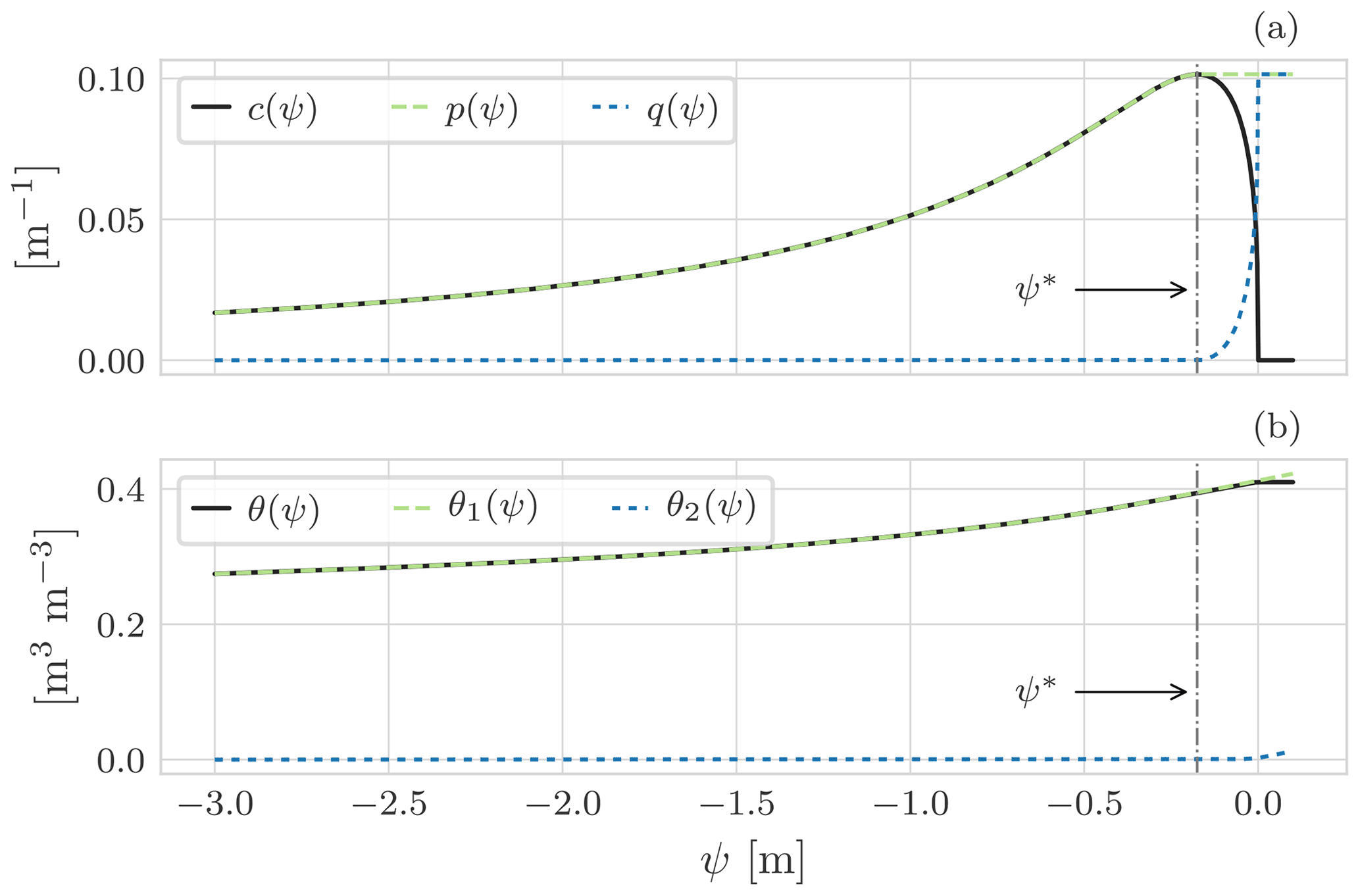
Figure 2 Graphical representation of the Jordan decomposition for soil water content using the SWRC model by Van Genuchten (1980) for a clay loam soil (Bonan, 2019). (a) The Jordan decomposition of c(ψ) as in Eq. (35). For $\mathit{\psi }={\mathit{\psi }}^{*}$, c(ψ) presents a maximum: for $\mathit{\psi }<{\mathit{\psi }}^{*}$ it is increasing, and for $\mathit{\psi }>{\mathit{\psi }}^{*}$ it is decreasing. This nonmonotonic behaviour causes problems when solving the nonlinear system. c(ψ) is thus replaced by p(ψ) (in green) and q(ψ) (in blue), which are two monotonic functions whose difference is the original function c. Consequently, (b) θ(ψ) is replaced by θ₁(ψ) and θ₂(ψ) (Eq. 36).

Instead, when we consider the water depth function to describe the computational node at the soil surface, the vectorial function is defined as V(ψ)=(θ_i(ψ_i)) for $i=\mathrm{1},\mathrm{2},\mathrm{\dots },N-\mathrm{1}$ and V_N(ψ)=H(ψ). Therefore, the nonlinear system in Eq. (38) is valid to describe both the subsurface and surface waters when the symbols are appropriately understood.

This aspect, the use of two different equation states, and the fact that the NCZ algorithm can be successfully re-used to solve other problems (Casulli and Zanolli, 2012; Tubini et al., 2021b), requires a careful design of its implementation, as discussed in the following sections.

3 Design and deployment of WHETGEO-1D

The concepts and requirements previously illustrated must be cast into software whose usability, expandability, and inspectability are demanded by good software design, which adds further requirements. The software design requirements and the software deployment are explained below.

3.1 Design requirements

One of the major difficulties encountered by a research group concerns the development and re-use of scientific software (Berti, 2000) and the writing of structurally clean code, i.e. a code that is easily readable and understandable, with objects that have a specified and possibly unique responsibility (Martin, 2009).

An object-oriented programming approach, with the adoption of standard design patterns (DPs) (Gamma et al., 1995; Freeman et al., 2004) and the creation of new ones, has been adopted for the internal class design and hierarchy.

The design principles followed by the WHETGEO-1D software can be summarized as follows.

• a.

  The software should be open-source to allow inspection and improvements by third parties.

• b.

  For the same reason it should be organized into parts, each with a clear functional meaning and possibly a single responsibility.

• c.

  The software can be extended with minimal effort and without modifications (according to the “open to extensions, closed to modifications” principle; Freeman et al., 2004). In particular, the parts to be modified are those that, according to the discussion in the previous sections, could be changed to try new closures, i.e. the SWRCs and the hydraulic conductivities in the case of the R² equation and the thermal capacity and thermal conductivity in the case of the energy budget. Adding a new SWRC type or a new conductivity function should be easy.

• d.

  The largest set of boundary conditions should be smoothly manageable.

• e.

  The implementation of equations should be abstract, according to the principle of “programming to interfaces and not to concrete classes”, which is the core of contemporary OOP (Gamma et al., 1995). The different equations describing the processes should be implemented within the set of classes by implementing a common interface.

• f.

  The implementation of algorithms should not depend on the data formats of inputs and outputs.

Another requirement has to do with the user experience. In fact, solvers of partial differential equations (PDEs) (Menard et al., 2020) tend to be complex to understand and run when features are added. In particular, the number of inputs grows exponentially when features are added, and the user has to overcome a steep learning curve before being able to use these software packages to appreciate all the cases implemented and their physics.

• g.

  To simplify this situation, WHETGEO-1D has to be implemented is such a way that any of the alternative implementations must come only with their own parameters and variables, as well as appear to the user to be as simple as possible, though not too simple.

There is finally a last requirement to consider.

• h.

  For computational and research purposes, there will be one-, two-, and three-dimensional (1D, 2D, 3D) implementations of the aforementioned equations. Therefore, as much of the code as possible should be shared across these. In particular, the NCZ and Newton algorithms should be shareable across the various applications.

This requirement implies that the geometry of the domain, as well as the topology, should be specified in an abstract manner to cope with the specifics of each dimensionality.

The rest of this section is organized to respond to points (a) to (h). Point (a) is actually responded to in the next section describing where the software can be downloaded and with which open license. Points (b) and (c) are accomplished by studying an appropriate design of classes and the use of design patterns (Gamma et al., 1995; Freeman et al., 2004). For (d), generic programming is used and specific classes are implemented. Point (e) is resolved by deploying a set of classes that implement a common interface with an extension that allows it to obtain the required functionalities.

To respond to the issues raised in (f) and (g), WHETGEO-1D is implemented as various components of OMS3, as shown below, each one with its own inputs. Therefore, the number of flags to check and the number of unused inputs are reduced to the minimum required by the solvers and parameterizations that the user chooses. If users want to solve the R² equation alone, for instance, they can pick out the appropriate component and do not need to know about the inputs and details of the energy budget. The separation into components has two other advantages. First, it eases the testing of a single process against available analytical solutions and against other model results (Bisht and Riley, 2019). Second, it improves the model structure, facilitating the representation of new processes (Clark et al., 2021).

Point (h) is solved by deploying new components for the 1D, 2D, and 3D cases. In the following section we mainly deal with points (b) to (e). Before discussing details of some classes, a few general choices have to be reported. Data of any type are stored internally in vectors of doubles, which in turn encapsulated in appropriate Java objects. OOP good practice would suggest that an object should be immutable (Bloch, 2001), but we decided that the main classes have to be mutable and allocated once forever as singletons (Gamma et al., 1995; Freeman et al., 2004). This potentially exposes the software to side effects but frees it to allocate new objects at any time step and decreases the computational burden and memory occupancy generated by deallocating unused obsolete objects at runtime. This approach may be considered a specific design pattern for partial differential equation solvers.

3.2 The software organization

The more visible effect of our choices is that we have built various OMS3 components.

• whetgeo1d-1.0-beta

• netcdf-1.0-beta

• closureequation-1.0-beta

• buffer-1.0-beta

• numerical-1.0-beta

Internally, the classes are assembled by using some interfaces and abstract classes, since WHETGEO-1D is coded using the Java language.

In order to improve the re-usability of the Java code we adopted a generic programming approach (Berti, 2000) that consists of decoupling of algorithm implementations from the concrete data representation while preserving efficiency. The generic approach has been balanced with domain-specific ones that can improve the computational efficiency of the software, as is the case of the previously mentioned Thomas algorithm used in 1D implementations.

Another requirement regards the division of software classes into three main groups, as the lack of a proper separation between the parameterization of physical processes and their numerical solutions has been recognized as one of the weak points of existing land-surface models (Clark et al., 2015b, 2021). One group describes the mathematical–physical problem, the second one implements the numerical solution (Berti, 2000), and the third one contains the growing group of concrete classes. The first group contains the SWRC, as well as hydraulic and thermal conductivity, and it forms a stand-alone library since its content can eventually be re-used in the 2D and 3D version of WHETGEO-1D. Similarly, we grouped the classes that solve linear and nonlinear algebraic systems, containing the Thomas conjugate gradient and the various Netwon types of algorithms, into a second stand-alone library. The third group of classes gathers the concrete implementations and the variety of OMS3 components that are deployed.

The classes used, and their repository for third-party inspection, are illustrated in the 00_Notebooks referred to in Sect. 4 and in the Supplement. However, there are three pivotal groups of classes that we want to mention here: these contain the description of the geometry of the integration domain, the closure equation, and the state equation.

3.2.1 Computational domain, i.e. the Geometry class

One of the key aspects to have in a generic solver regards the management of the grid and, in particular, the definition of its topology, or how grid elements are connected to each other. In the 1D case the description of the topology is quite simple since it can be implicitly contained in the vector representation: each element of the vector corresponds to a control volume of the grid, and it is only connected with the elements preceding and following it. It is worth noting that this approach is peculiar to 1D problems and cannot be adopted for the 2D and 3D domains, where, especially when unstructured grids are used, the grid topology requires a smart implementation of the incidence and adjacency matrices.

For each control volume it is necessary to store its geometrical quantities, their position and dimension, its variables, its parameter set, and the form of the equation to be solved there, referred to in the following as “equation state”. The appropriate arrangement of information, together with the internal design of the classes, allows us to create a generic finite-volume solver.

3.2.2 Closure equations, i.e. the ClosureEquation abstract class

The ClosureEquation class is shown in the Unified Modeling Language (UML) diagram in Fig. 3. As explained in the Introduction, one of the core concepts of modelling water and heat transport in soils is the SWRC. Soil is a multi-phase material, and thus knowledge of its composition is of crucial importance in defining its unsaturated hydraulic conductivity as well as its thermal properties, specific internal energy, and thermal conductivity.

An abstract class, ClosureEquation, is defined to contain only abstract methods that would be overwritten by the concrete classes implementing it. The ClosureEquation class essentially defines a new data type. A closer inspection of Fig. 3 reveals that the ClosureEquation is composed by aggregation with the Parameter class, which contains all the physical parameters of the model. Moreover, the Parameter class is implemented by using the Singleton pattern (Freeman et al., 2004). This design pattern is functional to have only one instance of the Parameter class shared by all the ClosureEquation objects and to provide a global point of access to the Parameter instance.

Figure 3 UML class diagram for the Java Simple Factory applied for the choice of the SWRC model. The ClosureEquation defines the interface that is implemented by the concrete classes SWRCVanGenucthen and SWRCBrooksCorey. The ClosureEquation is aggregated with the class Parameters containing the physical parameters of the model. Parameters is implemented by using the Singleton pattern, and its instance is inherited by the concrete classes SWRCVanGenucthen and SWRCBrooksCorey.

The Simple Factory pattern SoilWaterRetentionCurvesFactory accomplishes the task of implementing the concrete classes. By preferring polymorphism to inheritance and using the Simple Factory pattern (Gamma et al., 1995; Freeman et al., 2004), the developers can easily include and extend existing code or new formulations or parameterizations of SWRC. Also, the Simple Factory fulfils the dependency inversion principle (Eckel, 2003), and thus new extensions cannot affect the functioning of existing code. The same closure equation, for instance a particular SWRC, can be used to compute the soil water volume when solving the R² equation and the specific enthalpy of the soil when solving the heat equation.

3.2.3 Equation state, i.e. the EquationState class

The EquationState class in Fig. 4 contains the implementation of the discretized form of the equation state of the PDE under scrutiny. It contains a reference to the ClosureEquation object, the Geometry object, and the ProblemVariables object.

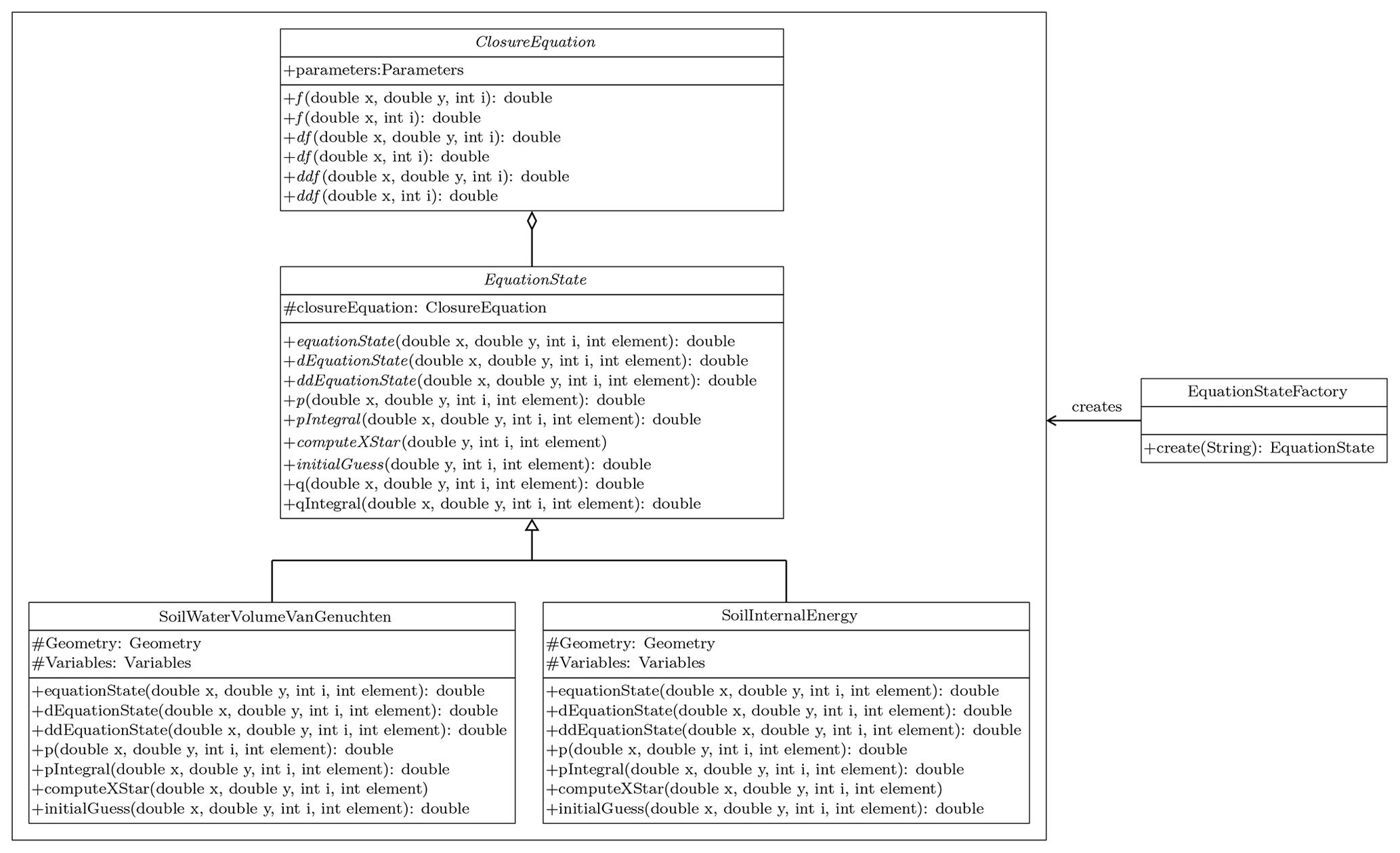
Figure 4 UML class diagram for the Java Simple Factory applied for the choice of the EquationState model. The EquationState defines the interface that is implemented by the concrete classes SoilWaterVolumeVanGenucthen and SoilInternalEnergy. The EquationState contains a reference to a ClosureEquation object.

Notably, the solver of a PDE problem can refer to the abstract class and to its abstract object without implying the specific concrete equation to be solved or its concrete parameterizations. Moreover, the compositionality of the EquationState allows the creation of new solvers from existing closures without the need to add new subclasses. As shown in the UML in Fig. 4, the EquationState class defines methods used to linearize the PDE when it is nonlinear. For instance, it computes the first and second derivatives and the functions necessary to define the Jordan decomposition as required by the NCZ algorithm. Specifically, these methods are p, q, pIntegral, qIntegral, and computeXStar.

In our code design the ClosureEquation class is limited to computing a physical parameterization, whereas the EquationState class is used to discretize the equation state of the PDE and whenever required to properly linearize it. Any new concrete EquationState subclass can either have the same physics of another with a different solver or different physics with the same solver.

3.3 Generic programming at work

As explained in Sect. 2.1.2, the definition of the surface boundary condition for the R² equation can require the introduction of an additional computation node at the soil surface to simulate the water depth. This means that we have two different equation states: one for the soil water content and one for the water depth. On the other hand, when considering the Neumann or Dirichlet boundary condition we have only one equation state for the soil water content. The nonlinear solver of the NCZ algorithm must work seamlessly with any type of boundary condition used and with any type of equation involved in the problem.

Let us consider, for example, the case of the R² equation with water depth as the surface boundary condition. Figure 5 reports the pseudocode for computing the nonlinear functions in the NCZ algorithm using a procedural approach. When traversing the computational grid we need to resort to an if-else statement to compute the nonlinear function of each control volume: the control volume N represents the control volume for the surface water, and in this case we need to use the water depth equation state, H(ψ) in Fig. 5. The remaining control volumes represent the soil moisture, and for them we need to use the SWRC equation state, θ(ψ) in Fig. 5. The main limit of this approach is that the computation of the nonlinear functions, H(ψ) and θ(ψ), is hard-wired into the code of the NCZ algorithm. This presents a shortcoming for the re-usability of the code since, as the boundary condition changes and the physical problem changes, it is necessary to modify the for loop and the name of the objects computing the nonlinear functions.

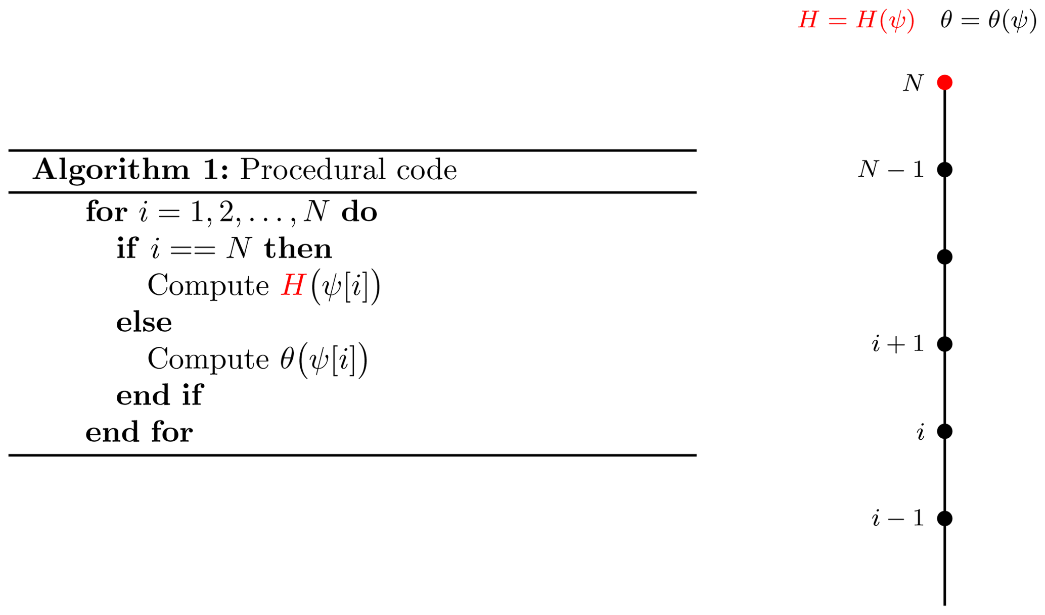
Figure 5 Adopting a procedural approach, the computation of the equation states is hard-wired into the code. The behaviour of each control volume is determined by an if-else statement according to the position of the element in the grid. In this case the properties of the grid, here the equation state, are joined with the topology. Here the nonlinear function V(ψ) is replaced with either H(ψ) or θ(ψ) according to the position of the node. To keep the pseudocode short, H(ψ) and θ(ψ) stand for all the nonlinear functions used in the NCZ algorithm, and the method f stands for one of the methods defined in the EquationState class.

Adopting the OOP and generic programming approach (Fig. 6), it is possible to implement the NCZ algorithm in such a way that enhances its re-usability. The key feature is the decoupling of the computational grid from the algorithm (data) (Berti, 2000). This is achieved through two elements. The first consists of creating a container of the objects that deal with the equation states of the problem, equationState, eS in Fig. 6. Second, we use a label equationStateID, eSID in Fig. 6, to specify the behaviour of each control volume. So, the behaviour of each control volume is determined by this label and not by the position of the element in the grid. Specifically, when we traverse the grid we use the equationStateID to determine which object inside the container equationState to use.

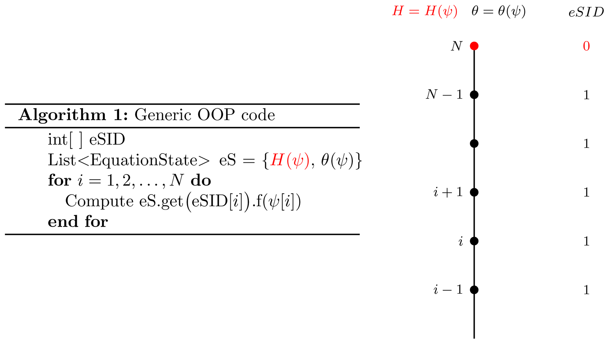
Figure 6 Adopting OOP with a generic programming approach, the computation of the equation states is independent from the grid. In fact, the behaviour of each control volume is determined by the vector eSID – equationStateID in the code – that determines which object belonging to the class EquationState of eS – equationState in the code – must be used to compute the equation state. In this manner it is possible to traverse the computation domain without resorting to the if-else statement. Here the nonlinear function V(ψ) is consistently replaced with either H(ψ) or θ(ψ) according to the position of the node. To keep the pseudocode short, H(ψ) and θ(ψ) stand for all the nonlinear functions used in the NCZ algorithm, and the method f stands for one of the methods defined in the class EquationState.

The NCZ algorithm has been implemented in the NestedNewtonThomas class. The NestedNewtonThomas contains a reference to the Thomas object, whose task is to solve a linear system, and to a list of EquationState objects (Fig. 7). Considering the ubiquity of nonlinear problems in hydrology and the robustness of the NCZ algorithm, the NCZ algorithm has been encapsulated in a stand-alone library.

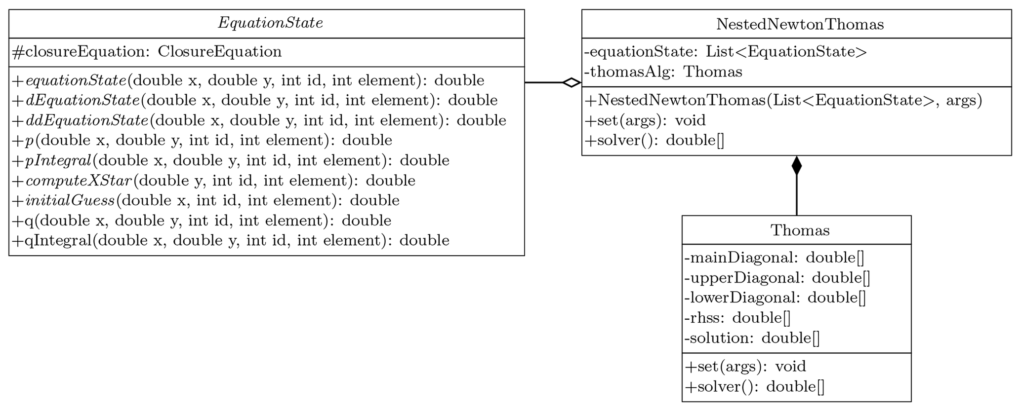
Figure 7 UML class diagram of the NestedNewtonThomas class. This class deals with the solution of the nonlinear system. The NestedNewtonThomas contains a reference to the Thomas object, whose task it is to solve a linear system, and to a list of EquationState objects.

The example has been illustrated in 1D, but it becomes even more effective when working in 2D or 3D, especially with an unstructured grid.

4 Information for users and developers

While most of what has been written so far is of general application, the deployment shown here is 1D. Information on WHETGEO-1D for users and developers is provided in the Supplement, where there is a Jupyter Notebook that contains the guidelines for executing the codes for any of the components. Its name starts with “00_”, and we call it “Notebook Zero” of the components. The latest executable code can be downloaded from

• https://github.com/geoframecomponents/WHETGEO-1D (last access: 21 December 2021)

and can be compiled by following the instructions therein. The version of the OMS3 compiled project can be found here: https://github.com/GEOframeOMSProjects/OMS_Project_WHETGEO1D (last access: 21 December 2021). The code can be executed in the OMS3 console, which can be downloaded and installed according to the instructions given at

• https://geoframe.blogspot.com/2020/01/the-winter-school-on-geoframe-system-is.html (last access: 21 December 2021).

Some brief information about GEOframe can be found in Appendix B, and more comprehensive information is at

• https://abouthydrology.blogspot.com/2015/03/jgrass-newage-essentials.html (last access: 21 December 2021) and

• https://geoframe.blogspot.com/2015/03/ (last access: 21 December 2021).

To run the tests, please follow the instructions on the GitHub repository of the GEOframe components. If a user wants to compile the code themselves, they can use the appropriate Gradle script that guarantees independence from any IDE.

For further information about input and output formats for WHETGEO-1D, please see the Notebook 00_WHETGEO1D_Richards.ipynb in the folder documentation of the Zenodo distribution.

4.1 Workflow for users

Examples of uses of WHETGEO-1D can be found in the form of Python Notebooks in the directory Notebooks/Jupyter. Documentation can be found in the form of Python Notebooks in the directory documentation. Simulations with WHETGEO-1D are run as OMS3 simulations. Therefore, the first operation to accomplish is to prepare the appropriate .sim files. For new users, many simulation files are available in the directory simulation of the Zenodo distribution. As shown in Fig. 8, in the modelling solutions that involve WHETGEO-1D, there is always a “main” component that is in charge of running the core code for solving the PDE. The inputs and the outputs are treated by other OMS3 components. They are tied together by a domain-specific language (DSL) based on Groovy. This allows for great flexibility in using various input and output formats.

4.2 Inputs and outputs

Input data can be broadly classified into time series, computational grid data, and simulation parameters. Time series are used to specify the boundary conditions of the problem. Time series are contained in .csv files with a specific format that is OMS3-compliant (David, 2021). With computational grid data we refer to the domain discretization, initial condition, and soil parameters. All these data are stored in a NetCDF file. Time series and computational grid data are elaborated with dedicated Python modules distributed under the geoframepy package (Tubini and Rigon, 2021a). The simulation parameters, such as the start date and end date of the simulation, time step size, and file paths, are specified by the user in the OMS3 .sim file.

For the design of the output workflow we took advantage of the OMS3 system that allows the user to connect stand-alone components. Figure 8 shows the output workflow for saving output data with Main, Buffer, and netCDF writer as the stand-alone OMS3 components. Main stands for the generic component having the responsibility of solving the PDE. Buffer has the responsibility of temporarily storing output data, and Writer handles the saving of data to the disk. The Buffer component has the sole purpose of storing data, and this has two important advantages. The first is that it limits the number of accesses to the disk to save output, i.e. reducing the computational time. The second is that it introduces a layer separating the Main component from the netCDF writer. This increases the flexibility of the modelling solution, as future developers can adopt different file formats or develop different writer components that, instead of saving all the outputs, can save discrete outputs or aggregated outputs. The advantage is that developers need only know the legacy of the Buffer component and customize both the output file format and memory optimization strategy, such as chuncking, according to their need. Currently all outputs are stored in a NetCDF-3 format (Unidata, 2021). NetCDF is a self-describing portable data format developed and maintained by UCAR Unidata. NetCDF is commonly used by the geoscience community, and there is an ever-growing number of tools for processing and visualization.

The choice of including the Buffer component in the workflow of the modelling solution is motivated by earlier experiences of the GEOtop community with the GEOtop model and by more recent experience with the FreeThaw1D model (Tubini et al., 2021b), according to which long spin-ups of the model (∼1500 years) were required with consequently large output files (∼ GB). Furthermore, in anticipation of the 2D and 3D developments, the NetCDF-3 format is probably not the most appropriate and could be abandoned in favour of more performing file formats (Unidata, 2021a, b), such as NetCDF-4 or HDF5.

Figure 8 Workflow of WHETGEO-1D. The boundary condition readers, computational grid reader, Main, Buffer, and netCDF writer are stand-alone OMS3 components. Main stands for the generic component with the responsibility of solving the PDE; the Buffer temporarily stores output data that are later passed to the netCDF writer component, which in turn saves data to the disk. The Buffer component has the sole purpose of storing data. This has two advantages: the first one is to limit the number of accesses to the disk to save output, i.e. reducing the computational time, and the second one is to introduce a layer separating the Main component, which handles the numerical solution of the PDE, and the component responsible for saving outputs.

WHETGEO-1D can be integrated with the built-in calibration component LUCA (Hay et al., 2006; Formetta et al., 2014a) and the Verification component, as shown in Fig. 9. The former is used to calibrate optimal parameters and the latter to compute the indices of goodness of simulated data versus measured data. Besides the LUCA component and the Verification component, it is necessary to add two more components, specifically the Buffer calibration parameters and the Measurement points data. The Buffer calibration parameters are needed to interface the Main component with the LUCA component. In fact, in the WHETGEO-1D Main component, physical parameters are stored as vectors, whilst LUCA handles calibration parameters as scalars (single value). The Buffer calibration component receives the optimal parameter set from the LUCA component and returns them packed in appropriate vectors. The Verification component receives as input two OMS3-compliant time series: one for measured data and one for simulated data. In this case it is necessary to extract from the simulation output only the simulated data at the measurement points of the variable used to calibrate the model. These data are then saved as OMS3 time series. It interesting that the integration of WHETGEO-1D with the OMS3 built-in calibration components is achieved by adding two new stand-alone components without modifying the source code of the existing components, i.e. the Main component, the Buffer component, and the netCDF writer.

Figure 9 Workflow of WHETGEO-1D integrated with LUCA. The cyan lines identify components required to integrate WHETGEO-1D with LUCA. The LUCA and Verification components are built-in OMS3 components. The former is used to calibrate optimal parameters and the latter to compute the indices of goodness of simulated data versus measured data. To integrate WHETGEO-1D with the OMS3 calibration components it is necessary to add two other components into the workflow, specifically the Buffer calibration parameters component and the Measurement points data component. LUCA handles scalar parameters, whilst WHETGEO-1D uses vectorial parameters. Buffer calibration parameters creates an interface between these two components, simply creating vectorial parameters from scalar parameters. The Verification component requires the input time series as a .csv file of simulated data at the measurement points. To accomplish this requirement, it is necessary to modify the output strategy: the Buffer component passes output data to the Measurement points data component. This component extracts only the simulated variables at the measurement points and passes them to the OMS3 time series writer, .csv writer, which saves the simulated time series as a .csv file. Notably, if the user is not interested in saving all the output of each run of the model during calibration, it is possible to remove the netCDF writer component.

4.3 Workflow for developers

Here, as an example, we present how to add the Brooks–Corey (Brooks and Corey, 1964) model as an extension of the code base. The constitutive relationships are given by

$$\begin{array}{}\text{(39)}& {\displaystyle }& {\displaystyle }\mathit{\theta }\left(\mathit{\psi }\right)=\left\{\begin{array}{ll}{\mathit{\theta }}_{\mathrm{r}}+({\mathit{\theta }}_{\mathrm{s}}-{\mathit{\theta }}_{\mathrm{r}}){\left(\frac{{\mathit{\psi }}_d}{\mathit{\psi }}\right)}^n& \text{if }\mathit{\psi }\le {\mathit{\psi }}_d\\ {\mathit{\theta }}_{\mathrm{s}}& \text{if }\mathit{\psi }>{\mathit{\psi }}_d\end{array}\right.,\text{(40)}& {\displaystyle }& {\displaystyle }K\left(\mathit{\psi }\right)=K_{\mathrm{s}}{\left[{\displaystyle \frac{\mathit{\theta }\left(\mathit{\psi }\right)-{\mathit{\theta }}_{\mathrm{r}}}{{\mathit{\theta }}_{\mathrm{s}}-{\mathit{\theta }}_{\mathrm{r}}}}\right]}^{\mathrm{3}+\frac{\mathrm{2}}{n}},\end{array}$$

where θ_s and θ_r are the saturated and residual values of the volumetric water content, respectively, ψ_d is the air-entry water suction value, n is the pore size distribution index, and K_s is the saturated hydraulic conductivity at saturation.

The standard approach to adding a new SWRC parameterization, here the Brooks and Corey model, requires the definition of a new class that extends the abstract class ClosureEquation. This new class, SWRCBrooksCorey, provides the implementation of the abstract methods defined in the super class ClosureEquation and inherits the association with the Parameters class. Specifically, the SWRCBrooksCorey class overrides the following methods:

• f calculates the water content for a given water suction value and set of parameters (Eq. 39);

• df calculates the first derivative of Eq. (39);

• ddf calculates the second derivative of Eq. (39).

In order to use the Brooks–Corey model in the Richards equation it is necessary to define a new class, SoilWaterVolumeBrooksCorey, that extends the abstract class StateEquation. Specifically, the SoilWaterVolumeBrooksCorey class overrides the following methods.

• equationState calculates the water volume using the Brook–Corey model for a given water suction value and set of parameters (Eq. 18).

• dEquationState calculates the first derivative of the equationState function, in case this the moisture capacity function. This method is used within the linearization algorithm.

• ddEquationState calculates the second derivative of the equationState function. This method is relevant for models for which the ψ^* cannot be computed analytically but requires the application of a root-finding method such as the bisection method. An example is the soil internal energy function when considering the phase change of water (Tubini et al., 2021b).

• p calculates the p function of the Jordan decomposition.

• pIntegral calculates the V₁ function of the Jordan decomposition.

• computeXStar calculates the ψ^* value to properly define the functions p and V₁.

• initialGuess calculates the initial guess for the linearization algorithm.

5 Conclusions

In this paper we discussed the issues raised by implementing a new expandable system to model the Earth's CZ, WHETGEO, the core of which is a reliable and robust integrator of the Richards–Richardson equation and the associated energy budget.

We would like to stress the following.

• WHETGEO makes available the NCZ algorithm, which has a priori convergence ensured for any choice of time step and for a great variety of boundary and initial conditions.

• The coupling between the R² equation and the heat advection diffusion equation is done using a recent algorithm (Casulli and Zanolli, 2005) that, to our knowledge, has not been applied before for the same scope.

• The application of our methods could benefit a large range of Earth science models, which at present require complicated workarounds (Regenass et al., 2021).

• The adoption of the mixed form of the equation allows the joint modelling of the saturated and unsaturated soil and groundwater conditions.

• Moreover, the coupling strategy with ponding water makes WHETGEO naturally suitable to investigate the partitioning of infiltration and surface runoff without any of the issues documented for other software (e.g. Šimůnek et al., 2005).

The implementation of WHETGEO has been shown to solve three software requirements and the (a) to (h) design specifications. Each of these was analysed and thus influenced the choice of algorithms and code implementation. Of the hydrological issues presented in seven observations, the issues 1 to 4 were also solved, and the code provided some answers for observations 5 to 7 because of the following.

• The code allows for the easy changing of soil water retention curves; therefore, for instance, it would be easy to implement new ones taking more accurate account of the different processes in the various ranges of suction. A description of how to add a new soil water retention curve is presented in Sect. 4.3.

• The effect of temperature on viscosity has been included, and, in the Supplement, we have shown that temperature changes in soil have relevant effects on infiltration and runoff production.

• Freezing and thawing processes coupled with the R² equation will be inserted. As an intermediate step, the heat conduction with phase change has been implemented in the energy budget solver.

The flexibility of the code was obtained with the creation of the 𝚂𝚝𝚊𝚝𝚎𝙴𝚚𝚞𝚊𝚝𝚒𝚘𝚗 and the 𝙲𝚕𝚘𝚜𝚞𝚛𝚎𝙴𝚚𝚞𝚊𝚝𝚒𝚘𝚗 classes, as illustrated in Sect. 3. Their organization can be considered a new programming pattern that can be re-used by programmers to implement the solution of partial differential equations independently of our use of the Java language. Furthermore, we also chose to implement the objects containing data by adopting the Singleton pattern. This choice violates the safety prescription that objects should preferably be immutable, but, by avoiding the continuous allocation and deallocation (through the Java garbage collector) of new objects, we aimed at saving computational time. Also, this scheme can be considered a design choice that can be replicated by anyone interested in scientific computing.

The first deployment of the concepts was the 1D stand-alone water budget as well as the coupled water and energy budget WHETGEO versions. The water budget was tested against analytical solutions presented in Srivastava and Yeh (1991) and Vanderborght et al. (2005). Some behavioural simulations were also performed to show some features of the code, such as the ability to deal with switching boundary conditions. Also, we showed that WHETGEO can be easily extended to simulate the thermal regime in frozen soils, as described in Tubini et al. (2021b), by merely adding the SFC model presented by Dall'Amico et al. (2011).

The model is an entirely new code that was accurately designed to allow easy inspection and to support code literacy and class re-use. It is open-source and built with open-source tools. It and its documentation fulfil the requirements of open science (Hall et al., 2021). In a science for which a lot of daily research activities are based on computer simulations, this is a requirement that most existing models do not fulfil but that the authors believe is profitable for the progress of science. Also, WHETGEO is built with a chain of open-source tools, making it available to all researchers who want to peruse it without constraint. Its documentation was produced using only open-source tools and is available together with the distribution of the main code.

Appendix A: GEOframe

WHETGEO-1D was implemented as a Java component within the GEOframe, an open-source, component-based hydrological modelling system. Within GEOframe, each part of the hydrological cycle is implemented in a self-contained building block, an OMS3 component (David et al., 2013). Components can be joined together to obtain multiple modelling solutions that can accomplish simple to very complicated tasks. GEOframe has shown great flexibility and robustness in several applications (Bancheri et al., 2020; Abera et al., 2017a, b). There are more than 50 components available that can be grouped into the following categories:

• geomorphic and DEM analyses;

• spatial extrapolation or interpolation of meteorological variables;

• estimation of the radiation budget;

• estimation of evapotranspiration;

• estimation of runoff production with integral distributed models;

• channel routing;

• travel time analysis;

• calibration algorithms.

Using the components for geomorphic and DEM analyses (Rigon et al., 2006b), the basin can be discretized into hydrological response units (HRUs), i.e. hydrologically similar parts, such as a catchment or a hillslope or one of its parts. The meteorological forcing data can be spatially interpolated using a geostatistical approach, such as the kriging technique (Bancheri et al., 2018). Both shortwave and longwave radiation components are available for the estimation of the radiation budget (Formetta et al., 2013, 2016). Evapotranspiration can be estimated using three different formulations: the FAO evapotranspiration model (Allen et al., 1998), the Priestley–Taylor model (Priestley and Taylor, 1972), and the Prospero model (Bottazzi, 2020; Bottazzi et al., 2021). Snow melting and the snow water equivalent can also be simulated with three models, as described in Formetta et al. (2014b). Runoff production is performed by using the Embedded Reservoir Model (ERM) or a combination of its reservoirs (Bancheri et al., 2020). The discharge generated at each hillslope is routed to the outlet using the Muskingum–Cunge method (Bancheri et al., 2020). Travel time analysis of a generic pollutant within the catchment can be done using the approach proposed in Rigon et al. (2016b, a). Model parameters can be calibrated using two algorithms and several objective functions: Let us calibrate (LUCA) (Hay et al., 2006) and particle swarm optimization (PSO) (Kennedy and Eberhart, 1995). A graph-based structure, called NET3 (Serafin, 2019), is employed for the management of process simulations. NET3 is designed using a river network and graph structure analogy, whereby each HRU is a node of the graph, and the channel links are the connections between the nodes. In any NET3 node, a different modelling solution can be implemented and nodes (HRUs or channels) can be connected or disconnected at runtime through scripting. GEOframe is open-source and helps the reproducibility and replicability of research (Bancheri, 2017). Developers and users can easily collaborate, share documentation, and archive examples and data within the GEOframe community.

Appendix B: OMS3

The Object Modelling System v.3 (OMS3) is a component-based environmental modelling framework that provides a consistent and efficient way to (1) create science simulation components; (2) develop, parameterize, and evaluate environmental models, as well as modify and adjust them as science advances; and (3) re-purpose environmental models for emerging customer requirements (David et al., 2013).

In OMS3 the term component refers to self-contained, separate software units that implement independent functions in a context-independent manner (David et al., 2013). This means that developers and researchers can build their model as a composition of stand-alone components, moving away from the monolithic approach. The entire GEOframe system, and therefore WHETGEO-1D, is built upon the OMS3 framework.

Compared to other environmental modelling frameworks (EMFs), OMS3 is characterized by being a noninvasive and lightweight framework (Lloyd et al., 2011). That is to say that the model code is not tightly coupled with the underlying framework – OMS3; i.e. the environmental modeller does not need a deep knowledge of the API, and the modelling components can still function and continue to evolve outside the framework (David et al., 2013). In fact, OMS3 relies on specific annotations to provide metadata for Java code. These annotations describe elements such as classes, fields, and methods and are used by the framework to interpret the component as a building block of the modelling solution (MS), hence controlling its connectivity and data flow (David et al., 2013). It is worth noting that, being metadata, these annotations do not directly affect the execution of the source code outside the OMS3 noninvasive and lightweight framework.

Besides the technical aspects, the adoption of a software framework has a positive effect on “nonfunctional” quality attributes, such as maintainability, portability, re-usability, and understandability (David et al., 2013). The component-based approach allows the developer to break down the problem into smaller parts, each one tackled by a specific component. Hence, the components are joined together to build the desired modelling solution (point b). This facilitates the construction of new MSs, thanks to the plug-in system of model components (David et al., 2013; Peckham et al., 2013; Serafin, 2019). Thanks to the modularity, the updating of a component with the most recent scientific advances is facilitated and has no side effects on the other components. The other advantage regards the long-term development of the code. From past experiences, one of the main limits to model development and maintenance was related to the lack of a proper software architectural design (Rizzoli et al., 2006; David et al., 2013; Formetta et al., 2014a; Bancheri, 2017; Serafin, 2019). Moreover, it is interesting to note that the component-based approach encourages collective model development (Serafin, 2019) and also eases the attribution of authorship since any component is a stand-alone chunk of code and can be authored separately.

Also, the adoption of an environmental modelling framework promotes the concept of reproducible research, easing third-party inspection and providing consistent and verifiable model results (Formetta et al., 2013; Bancheri, 2017; Serafin, 2019).

Another advantage of using OMS3 is represented by the opportunity to keep the code development transparent to the user.

Appendix C: R² test cases

In this section we test the solver of the R² equation against the analytical solutions presented by Srivastava and Yeh (1991) and by Vanderborght et al. (2005). Then we present and discuss two “behavioural” test cases to try out WHETGEO-1D in simulating both the infiltration excess and the saturation excess process.

C1 Analytical solution Srivastava and Yeh (1991)

Srivastava and Yeh (1991) derived an analytical solution describing the one-dimensional transient infiltration in a homogeneous and layered soil. The hydraulic properties of the soil are described by the following constitutive relations:

$$\begin{array}{}\text{(C1)}& {\displaystyle }K\left(\mathit{\psi }\right)=K_{\mathrm{s}}{e}^{\mathit{\alpha }\mathit{\psi }},\text{(C2)}& {\displaystyle }\mathit{\theta }\left(\mathit{\psi }\right)={\mathit{\theta }}_{\mathrm{r}}+({\mathit{\theta }}_{\mathrm{s}}-{\mathit{\theta }}_{\mathrm{r}})e^{\mathit{\alpha }\mathit{\psi }},\end{array}$$

where K_s is the saturated hydraulic conductivity, θ_r is the residual water content, θ_s is the saturated water content, and α is the soil pore size distribution parameter representing the desaturation rate of the SWRC. The lower boundary condition is represented by the water table, ψ=0, while the upper boundary condition is subjected to a constant flux, q. The initial condition corresponds to the steady-state profile due to a prescribed initial flux at the soil surface and prescribed pressure at the lower boundary. The analytical solution is derived by linearizing the Richards equation and using Laplace transformation. Details on the analytical solution can be found in Srivastava and Yeh (1991).

C1.1 Homogeneous soil

We consider a one-dimensional homogeneous soil layer of 1 m depth (TP1). The saturated hydraulic conductivity value is assumed to be 1.0 cm h⁻¹, with θ_s=0.45 m³ m⁻³, θ_r=0.2 m³ m⁻³, and α=0.01 cm⁻¹. The initial condition is determined by imposing as a lower boundary condition ψ=0 m and a constant water flux at the soil surface of q_A=0.1 cm h⁻¹. For times greater than 0 the water flux at the soil surface is q_B=0.9 cm h⁻¹. The domain is discretized with a uniform grid space Δz=0.001 m and the time step is Δt=60 s. The model accuracy is enhanced by allowing two Picard iterations per time step. Figure C1 shows a comparison between the numerical and the analytical solutions.

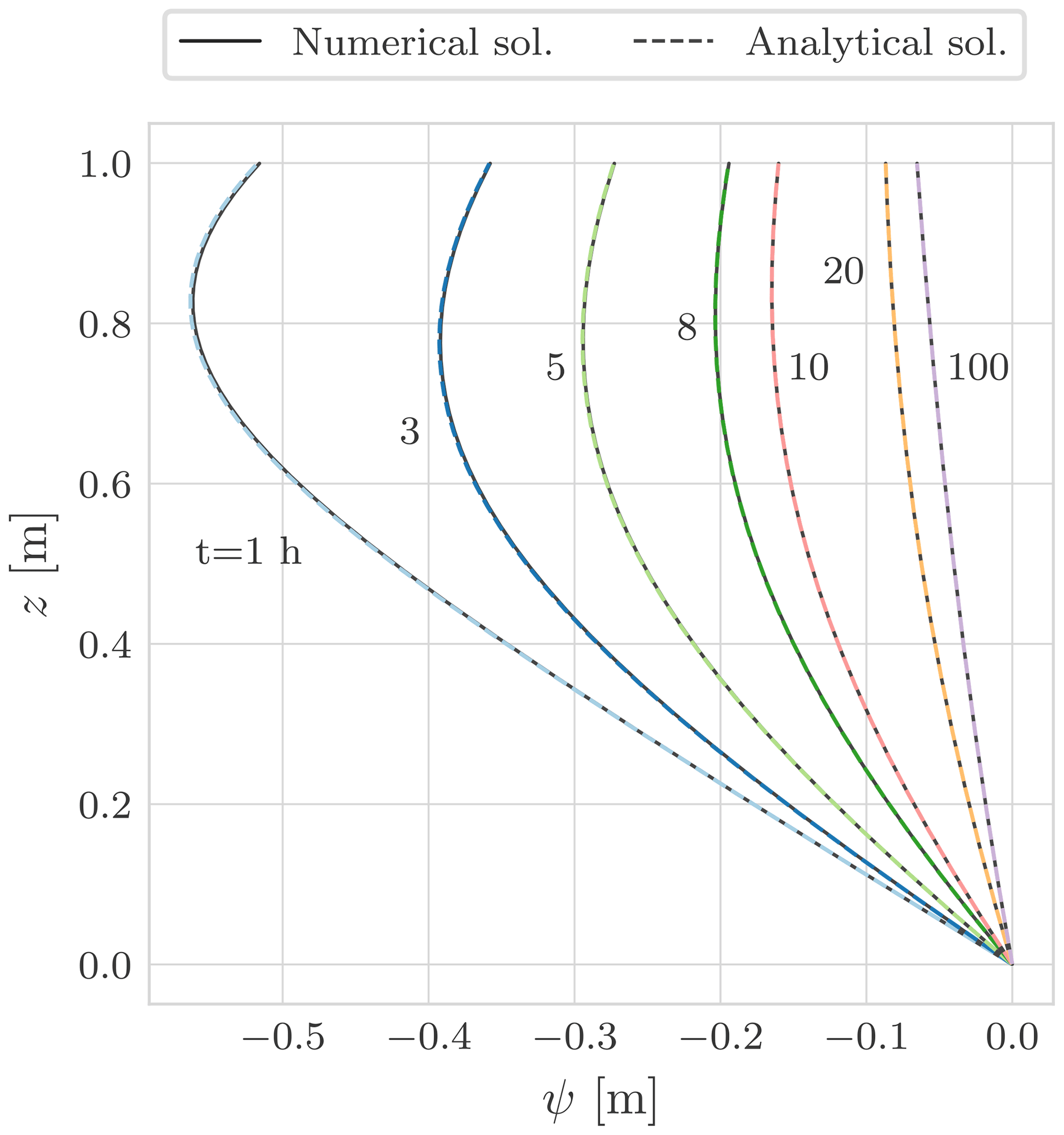
Figure C1 Comparison between the analytical and numerical solutions for the test problem TP1.

Figure C2 Relative water suction error for the test problem TP1.

C1.2 Layered soil

In this numerical problem (TP2) we consider one-dimensional vertical infiltration toward the water table through a layered soil. The initial condition is determined by imposing as a lower boundary condition ψ=0 m and a constant water flux at the soil surface of q_A=0.1 cm h⁻¹. For times greater than 0 the water flux at the soil surface is q_B=0.9 cm h⁻¹. The domain is discretized with a uniform grid space Δz=0.001 m and the time step is Δt=60 s. The model accuracy is enhanced by allowing two Picard iterations per time step. The hydraulic conductivity at the interface is computed as the harmonic mean of the neighbours (Romano et al., 1998). Comparison between the numerical and the analytical solution for water suction is shown in Fig. C3.

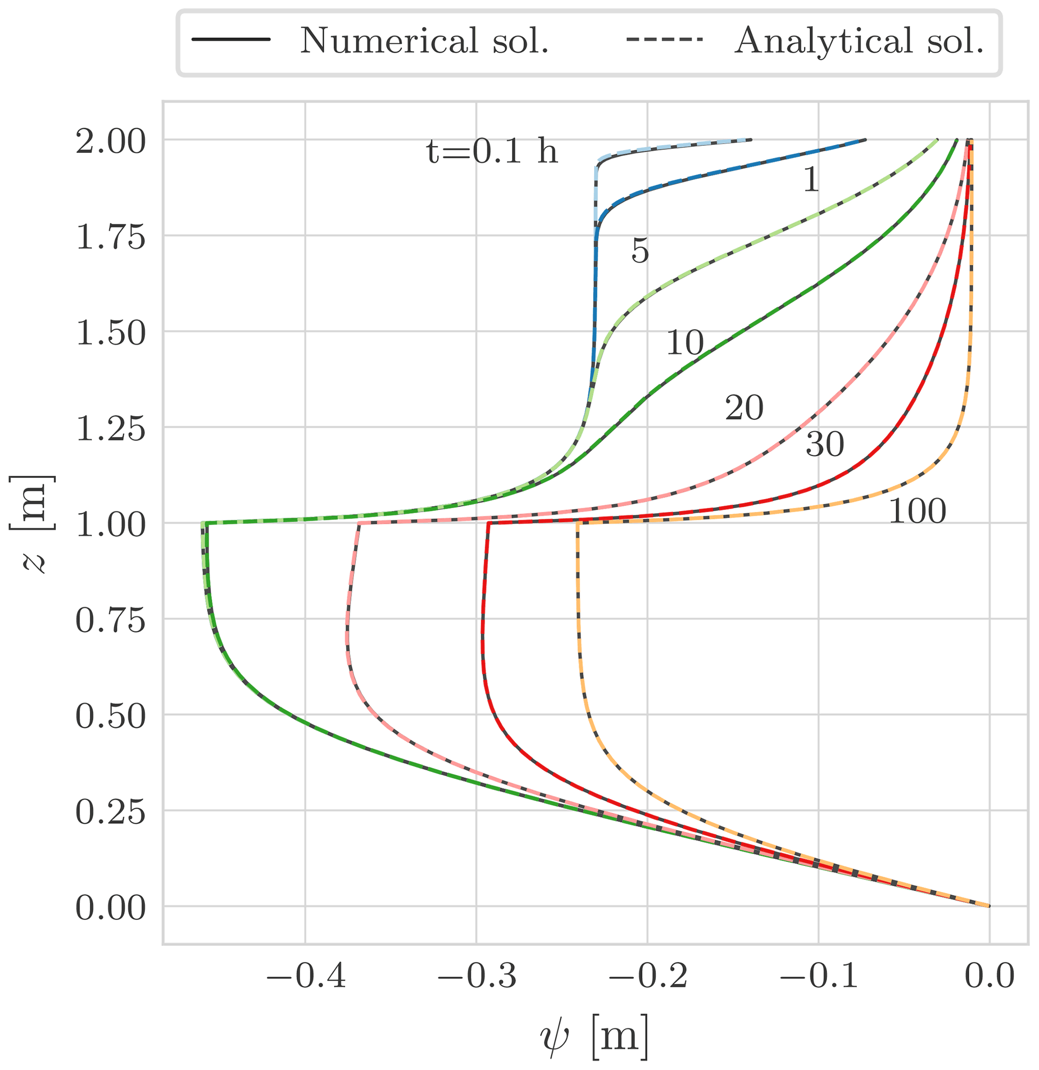
Figure C3 Comparison between the analytical and numerical solutions for the test problem TP2.

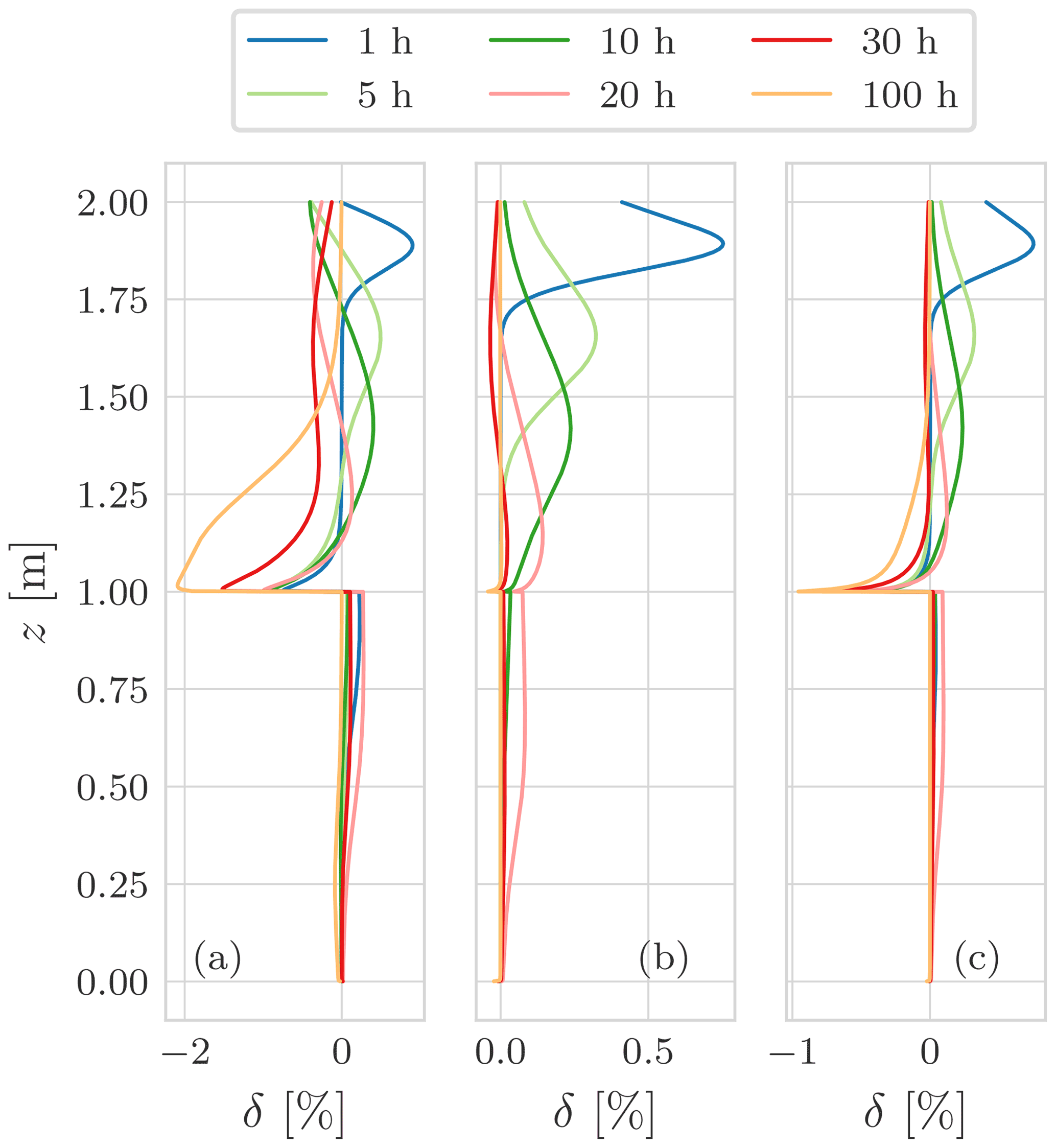
Figure C4 Comparison of relative water suction error δ for the test problem TP2 using different interface hydraulic conductivity algorithms. (a) Computed with max, (b) with harmonic mean, and (c) with geometric mean. As reported in Romano et al. (1998), the harmonic mean offers the best agreement with the analytical solution. This is particularly evident at the interface between the two layers.

C2 Analytical solution of Vanderborght et al. (2005)

The next test case was defined by Vanderborght et al. (2005) to evaluate the steady-state flux in layered soil profiles. For this numerical problem (TP3) we consider a soil column of 2 m depth with one soil type for depth 0–0.5 m overlying another soil type for depth 0.5–2 m, specifically for loam over sand, sand over loam, and clay over sand. The soil parameters are defined in Table C1. The initial condition for water suction is a uniform profile with $\mathit{\psi }=-\mathrm{20}$ m, the surface boundary condition is a constant flux of $q=\mathrm{5.79}\times {\mathrm{10}}^{-\mathrm{8}}$ m s⁻¹, and at the bottom we impose a free drainage boundary condition. The domain is discretized with a uniform grid space Δz=0.01 m and the time step is Δt=3600 s. In order to reach the steady-state condition the simulation lasts 2 years. Comparison between the numerical and the analytical solution is shown in Fig. C5.

Table C1 Hydraulic properties for the three soil types used in the Vanderborght test case (TP3).

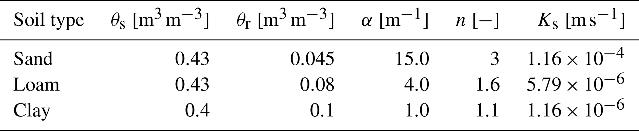
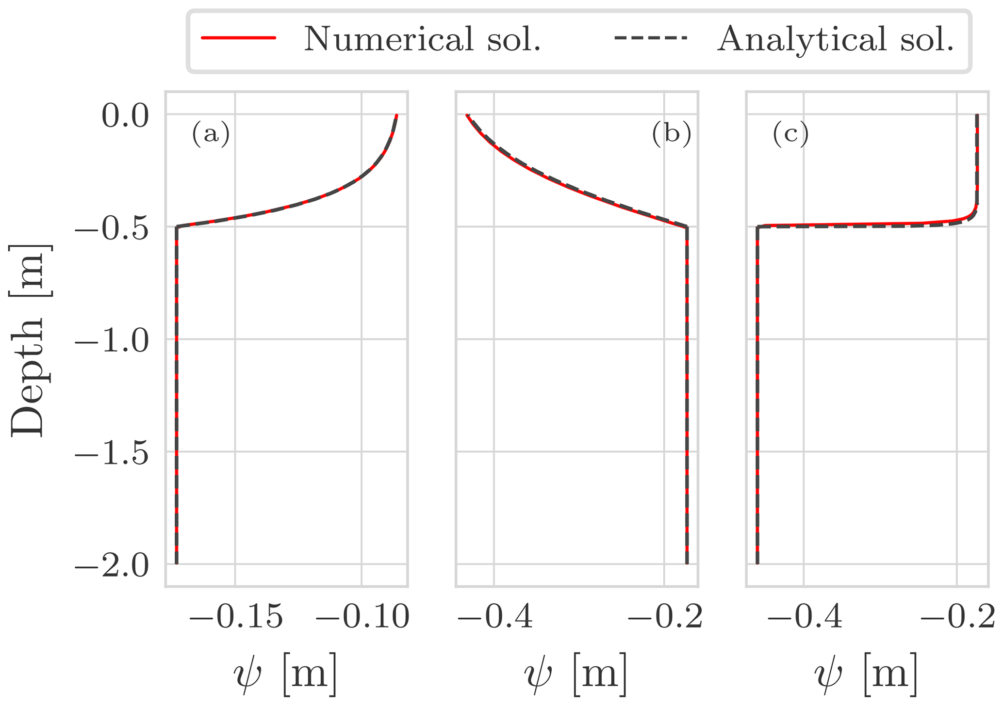
Figure C5 Comparison between the analytical and the numerical solution for the test problem TP3. The three panels show the vertical profile of water suction at steady state for a constant flow rate of $\mathrm{5.79}\times {\mathrm{10}}^{-\mathrm{8}}$ m s⁻¹: (a) clay–sand soil profile, (b) loam–sand soil profile, and (c) sand–loam soil profile.

C3 Surface boundary condition

The definition of the surface boundary condition is a nontrivial task since it is a system-dependent boundary condition. The infiltration rate through the soil surface depends on precipitation, rainfall intensity J, and on the moisture condition of the soil. Because of this, the surface boundary condition may change from the Dirichlet type – prescribed water suction – to the Neumann type – prescribed flux – and vice versa. The works by Horton (1933) and Dunne and Black (1970) establish the conceptual framework to explain the runoff generation.

The infiltration excess or Horton runoff occurs when the rainfall intensity is larger than the infiltration capacity of the soil:

$$\begin{array}{}\text{(C3)}& \left|J\right|>|-K(\mathit{\psi }\left){\displaystyle \frac{\partial }{\partial z}}\right(\mathit{\psi }+z){|}_{z=\mathrm{0}}.\end{array}$$

Infiltration excess is most commonly observed with short-duration, intense rainfall.

The saturation excess or Dunnian runoff occurs when the soil is saturated and additional water exfiltrates at the soil surface. Saturation excess generally occurs with long-duration, moderate rainfall or with a series of successive precipitation events. In this case the soil depth or the presence of shallow fragipan is the determining factor for saturation excess. Another possible cause is the rise of the water table up to the soil surface.

C3.1 Infiltration excess

In this numerical experiment we consider a homogeneous soil of 3 m depth. Soil hydraulic properties are described with the Van Genuchten model (Table C2).

Table C2 Hydraulic properties of the silty clay loam soil (Bonan, 2019) for the Horton runoff numerical experiment.

The initial condition is assumed to be hydrostatic with ψ=0 m at the bottom. The surface boundary condition is synthetic rainfall, as in Fig. C6a, lasting 15 min with constant intensity of 0.028 mm s⁻¹. At the bottom we prescribed a Dirichlet boundary condition with constant ψ=0 m so the transient is driven only by the surface boundary condition. In Fig. C6a, the time is indicated when it would be necessary to switch from the Neumann-type to the Dirichlet-type boundary condition.

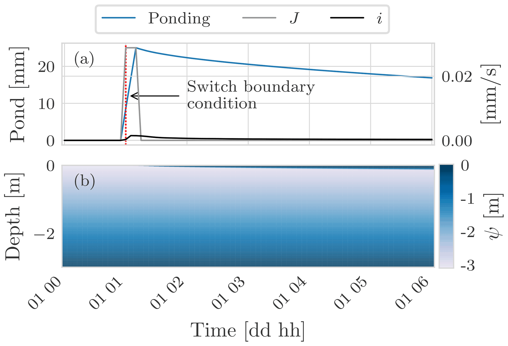
Figure C6 (a) A comparison between the rainfall intensity J and actual soil infiltration i. The rainfall intensity exceeds the actual infiltration rate so water builds up at the soil surface (blue line). (b) The time evolution of the water suction within the soil. From the numerical point of view, as water builds up at the soil surface it would be necessary to switch the boundary condition from Neumann type to Dirichlet type.

Figure C7 shows a comparison of water ponding at the soil surface considering two different initial conditions of the soil: wet and dry. For the wet case, the initial condition is hydrostatic with ψ=0 m at the bottom. For the dry case, the initial condition is hydrostatic with $\mathit{\psi }=-\mathrm{100}$ m at the bottom. In the wet initial condition the hydraulic conductivity is higher than for the dry initial condition; however, in the dry case the capillary gradient is larger and because of this the soil infiltration capacity is higher, as in Fig. C7a. With regards to the water ponding, the maximum value is almost the same in both cases, 1 mm higher in the wet case, but the time evolution is different: in the wet case the water only infiltrates completely 13 h later than the dry case. This delay may seem counter-intuitive since wetter conditions are associated with higher values of hydraulic conductivity (Fig. C8), but in the wet soil the capillary gradients are smaller than in the dry soil (Fig. C9).

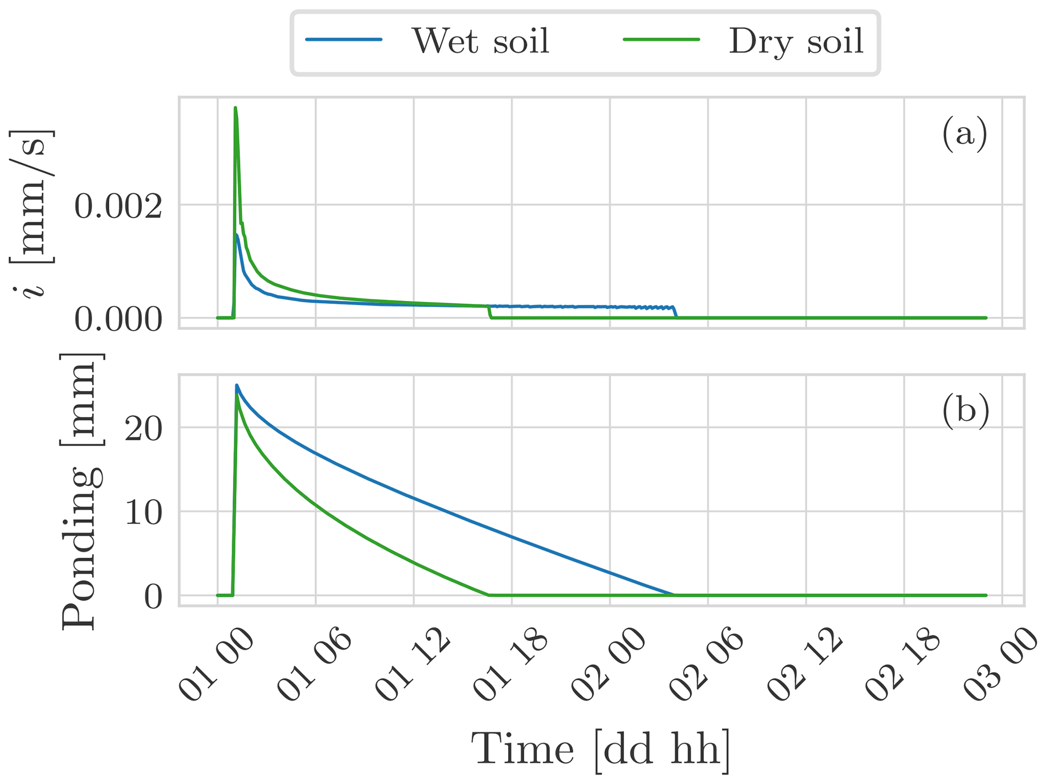
Figure C7 (a) A comparison between the infiltration rate for two cases: wet and dry initial condition. In the dry case, soil infiltration is greater than the wet case even though the hydraulic conductivity is smaller. This is due to the higher capillary gradients that develop in the soil. (b) The time evolution of the water ponding at the soil surface.

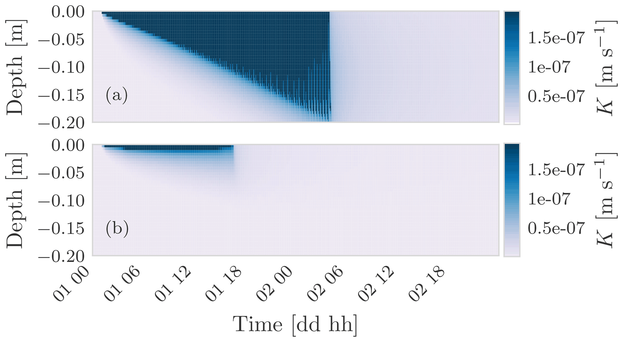
Figure C8 (a) The hydraulic conductivity field for the case of wet soil and (b) the hydraulic conductivity field for the case of dry soil.

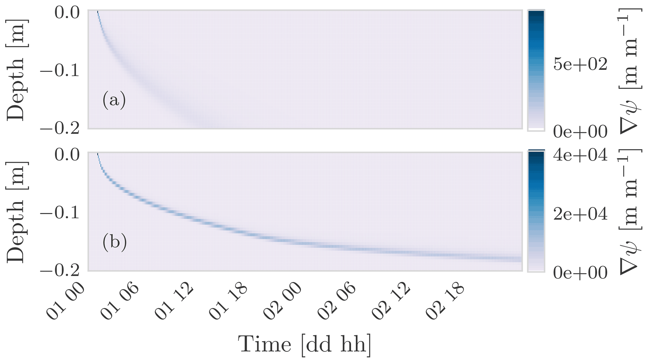
Figure C9 (a) The capillary gradient for the case of wet soil and (b) the capillary gradient for the case of dry soil. As can be seen, in the dry soil the capillary gradient is 2 orders of magnitude larger than in the wet soil. Because of this higher gradient water infiltrates faster in the dry soil than in the wet soil.

C3.2 Saturation excess

In this section we present two numerical experiments to simulate the saturation excess process. Saturation excess is more critical, in terms of simulation stability, than the infiltration excess (PC Progress Discussion Forums, 2021). We consider two cases: one in which the water table reaches the soil surface and another in which the total rainfall amount is larger than the maximum water-holding capacity but the rainfall intensity is less than the maximum infiltration rate.

Firstly, we consider a layered soil of 3 m depth. The thicknesses of the loamy layer and clay layer are 0.5 and 2.5 m, respectively. The soil hydraulic properties are described with the Van Genuchten model (Table C3). The initial condition is assumed to be hydrostatic with ψ=0 m at the bottom. At the surface boundary condition we prescribe no rainfall, while at the bottom a variable Dirichlet boundary condition is prescribed (Fig. C10a). The transient is driven by variation of the water table. In Fig. C10a the time is indicated when it would be necessary to switch the surface boundary condition from the Neumann-type to the Dirichlet-type boundary condition and vice versa.

Table C3 Hydraulic properties of the loam layer and clay layer in Bonan (2019) for the numerical experiment on Dunnian runoff due to water table rising.

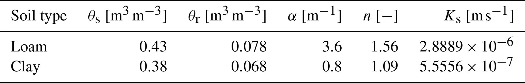
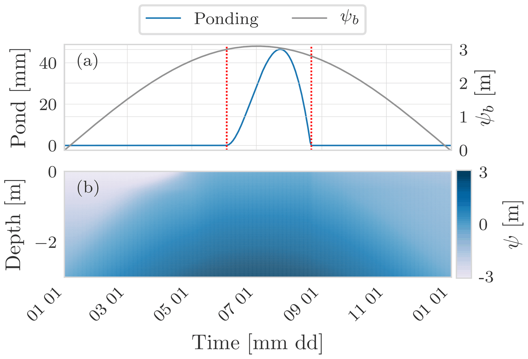
Figure C10 (a) The water table position, Dirichlet boundary condition, and the water ponding at the soil surface. The dotted red lines indicate the times at which the boundary condition at the soil surface should be switched. The first line indicates the switch from the Neumann type to the Dirichlet type since water starts building up. The second line indicates the switch form the Dirichlet type to the Neumann type because there is no water at the soil surface. (b) The time evolution of the water suction within the soil.

Table C4 Hydraulic properties of the loamy sand layer and clay layer in Bonan (2019) for the numerical experiment on Dunnian runoff due to rainfall.

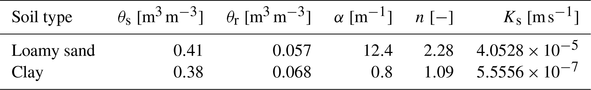
Secondly, we consider a layered soil of 3 m depth. The thicknesses of the loamy sand layer and the clay layer are 0.3 and 2.7 m, respectively. The soil hydraulic properties are described with the Van Genuchten model (Table C4). The initial condition is assumed to be hydrostatic with $\mathit{\psi }=-\mathrm{2}$ m at the bottom. The surface boundary condition is synthetic rainfall (Fig. C11a), and at the bottom we prescribed a Dirichlet boundary condition with constant $\mathit{\psi }=-\mathrm{2}$ m so the transient is driven only by the surface boundary condition. Figure C11b shows the time evolution of the degree of saturation within the soil. Initially water infiltrates into the soil but then the clay layer, which is characterized by a lower conductivity than the loam–sand layer, limits the deep infiltration causing the saturation of the loam–sand layer from below.

Figure C11 (a) The rainfall and the water ponding at the soil surface. Initially rainfall can infiltrate into the soil and no water builds up at the soil surface. As the uppermost layer of the soil saturates water starts ponding at the soil surface. The dotted red lines indicate the times at which the boundary condition at the soil surface should be switched. (b) The time evolution of the saturation degree within the soil.

Repeating the above numerical experiment with a thicker loam–sandy layer (Fig. C12), there is no water ponding at the soil surface. In this case all the rainfall can infiltrate into the loam–sandy layer thanks to the increased water storage capacity.

Figure C12 In this numerical experiment there is no saturation excess since the greater thickness of the uppermost layer ensures sufficient water storage capacity for the forcing rainfall.

Appendix D: Energy budget

Here we present a behavioural test case on the pure heat conduction considering the surface energy balance. The purpose of this simulation is twofold. First, we show an application of WHETGEO-1D that exploits existing GEOframe components to model the external components of the surface energy budget, specifically the incoming shortwave radiation (Formetta et al., 2013), the incoming longwave radiation (Formetta et al., 2016), and the latent heat flux. Second, we show how to easily include the phase change of water by adding a new closure equation that describes the SFC model presented by Dall'Amico et al. (2011)

The soil column is 30 m deep, and the initial condition is a constant temperature profile T=12 ^∘C. Figure D1a shows the components of the surface energy fluxes and the thermal regime of the uppermost 2 m of the soil column. As can be seen in panel (b), the soil temperature falls below 0 ^∘C; therefore, it is not reasonable to neglect freezing and thawing processes.

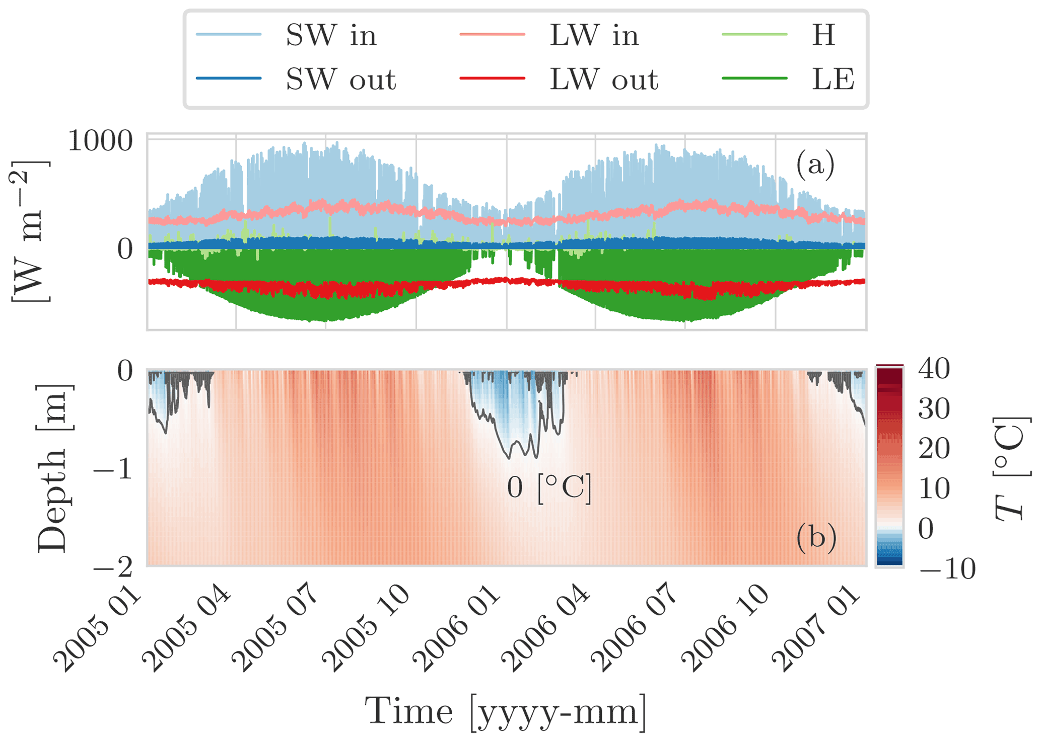
Figure D1 Behavioural test case of pure heat conduction in soil considering the surface energy budget. (a) The surface energy fluxes driving the simulation. The external fluxes, incoming shortwave and longwave radiation, and the latent heat flux are computed with existing GEOframe components. (b) The thermal regime of the uppermost 2 m of the soil column. As can be seen, during winter the temperature of the uppermost layer goes below 0 ^∘C, and the grey line is the 0 ^∘C isotherm; therefore, it is not reasonable to overlook the phase change of water.

Table D1 Parameters of the SFC model.

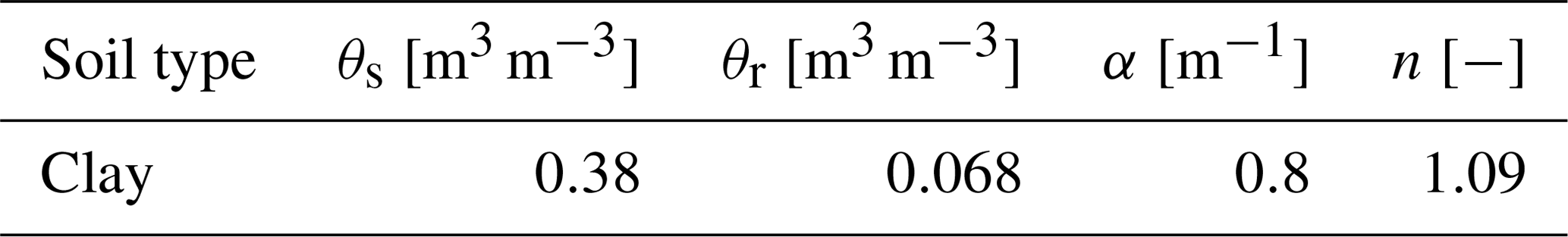
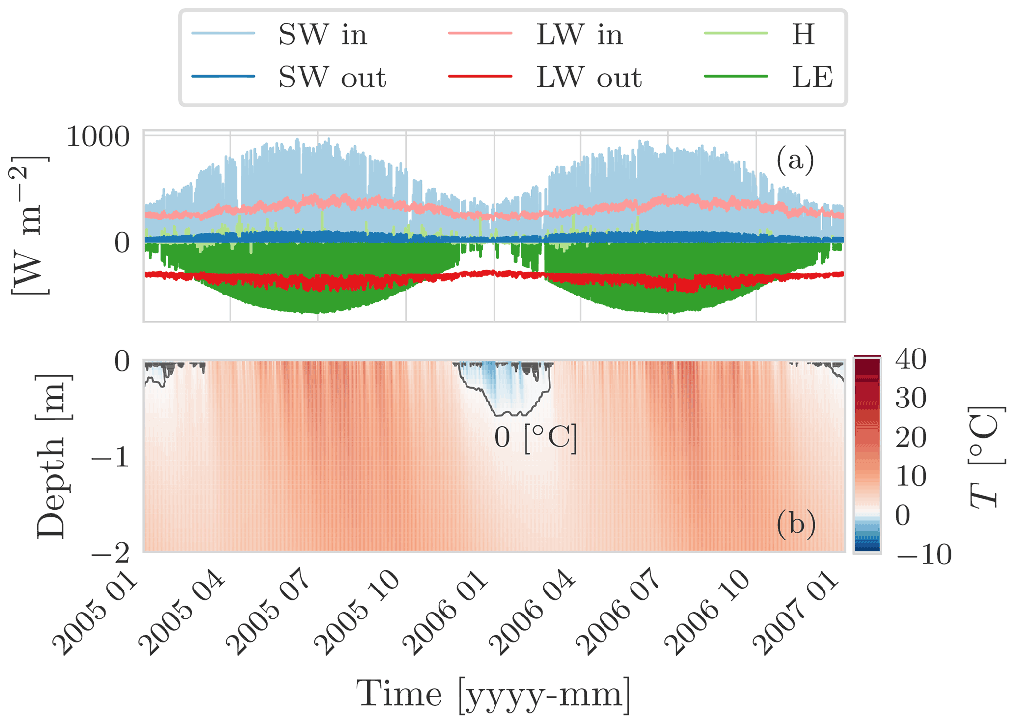
Figure D2 Behavioural test case of pure heat conduction in soil considering the surface energy budget and the phase change of water. (a) The surface energy fluxes driving the simulation. The external fluxes, incoming shortwave and longwave radiation, and the latent heat flux are computed with existing GEOframe components. (b) The thermal regime of the uppermost 2 m of the soil column.

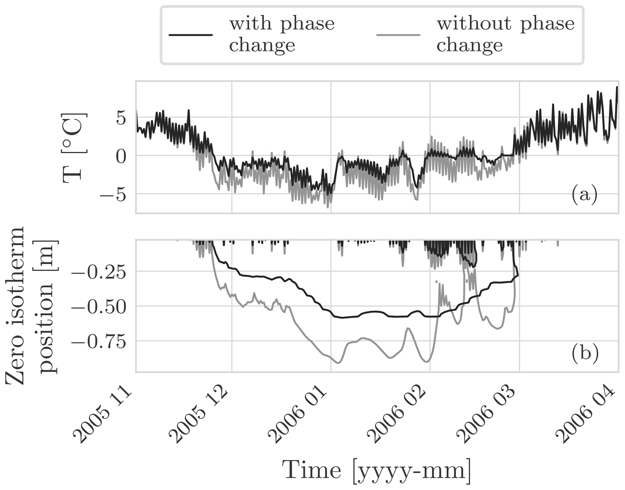
Figure D3 (a) A comparison of the soil temperature at 0.05 m with the phase change of water and without. As can be seen, in the latter case the soil temperature reaches a lower value and fluctuates more: when considering the phase change of water we include in the problem the latent heat of water that increases the thermal inertia of the soil. (b) A comparison of the position of the zero isotherm in the two simulations. When the phase of water is not included the zero isotherm goes deeper into the ground.

By including the closure equation of the SFC presented by Dall'Amico et al. (2011), it is possible to consider the phase change of water. Moreover, compared to the FreeThaw-1D model (Tubini et al., 2021b), in WHETGEO-1D it is possible to drive the simulation of the soil thermal regime by using the surface energy budget. This aspect represents a novelty with respect to FreeThaw-1D and was obtained with minimum effort thanks to the code design we adopted. The soil column is of 30 m depth, and the initial condition is a constant temperature profile T=12 ^∘C. The parameters of the SFC are presented in Table D1. Figure D1 shows in panel (a) the components of the surface energy fluxes and the thermal regime of the uppermost 2 m of the soil column. As can be seen in panel (b), the soil temperature falls below 0 ^∘C, and thus neglecting freezing and thawing processes results in a strong approximation.

Figure D3 shows a comparison between the two simulations.