TriCCo v1.1.0 – a cubulation-based method for computing connected components on triangular grids

We present a new method to identify connected components on triangular grids used in atmosphere and climate models to discretize the horizontal dimension. In contrast to structured latitude–longitude grids, triangular grids are unstructured and the neighbors of a grid cell do not simply follow from the grid cell index. This complicates the identification of connected components compared to structured grids. Here, we show that this complication can be addressed by involving the mathematical tool of cubulation, which allows one to map the 2-D cells of the triangular grid onto the vertices of the 3-D cells of a cubical grid. Because the latter is structured, connected components can be readily identified by previously developed software packages for cubical grids. Computing the cubulation can be expensive, but, importantly, needs to be done only once for a given grid. We implement our method in a Python package that we name TriCCo and make available via pypi, gitlab, and zenodo. We document the package and demonstrate its application using simulation output from the ICON atmosphere model. Finally, we characterize its computational performance and compare it to graph-based identifications of connected components using breadth-first search. The latter shows that TriCCo is ready for triangular grids with up to 500 000 cells, but that its speed and memory requirement should be improved for its application to larger grids.

1 Introduction

Climate and atmospheric modeling is experiencing a leap in its ability to represent the earth digitally (Satoh et al., 2019; Wedi et al., 2020). The leap is made possible by a drastic increase in spatial resolution and the development of global storm-resolving models that apply local differencing schemes and discretize the sphere by means of unstructured grids. An example of the latter is the triangular grid based on the icosahedron and applied in the ICON unified weather and climate model (Zängl et al., 2015; Giorgetta et al., 2018). The triangular grid is a defining difference of ICON from its predecessor models ECHAM and COSMO, which were based on latitude–longitude grids.

While having many numerical advantages, the change from a structured latitude–longitude to an unstructured triangular grid challenges established workflows and analysis methods. For some types of analysis, one might accept to interpolate the model output to latitude–longitude coordinates. For others, however, an interpolation might be problematic, as it artificially smoothes the boundary of objects, thereby potentially introducing an ambiguity into object-based analyses.

One analysis that is ideally done on the native model grid is connected component labeling. In atmospheric sciences, connected component labeling is applied for object-based studies of atmospheric moisture, clouds, and their topology. For example, previous works used it to characterize large-scale moisture transport in the form of atmospheric rivers (Muszynski et al., 2019) and to study clusters of convective clouds (Neggers et al., 2003; Rieck et al., 2014; Rempel et al., 2017; Licón-Saláiz et al., 2020), whose size statistics and distance to neighbors impact cloud behavior, cloud organization, and cloud radiative effects (Schäfer et al., 2016; Jakub and Mayer, 2017). With atmosphere and climate models moving to storm-resolving resolutions of a few kilometers or finer, three-dimensional radiative effects of clouds are becoming increasingly important. Because the radiative properties of clouds differ strongly from those of their surrounding air, a connected component labeling that respects the sharp boundaries between cloudy and cloud-free air seems especially important.

When connected component labeling is done on structured latitude–longitude grids, one has access to widely used analysis tools such as opencv (Bradski, 2000) and scikit-image (van der Walt et al., 2014) that are well documented and easily found. This comfort is lost when working on triangular grids. In fact, this loss has sparked our collaboration, which addresses a need from climate modeling (A. V.) and draws on expertise from pure mathematics (P. S.). Before we started our collaboration, one of us (A. V.) had – without much success – sought advice from some colleagues in climate science and visualization science regarding a tool for connected component labeling on a triangular grid. When revising the paper, and thanks to the input of the reviewers, it became clear to us that graph-based solutions provide such a tool (see Sect. 5). But the fact that this was clear neither to us nor to our colleagues is, in our view, an anecdotal illustration of how unstructured triangular grids challenge traditional workflows in climate science, which have been used for many decades and now need to be revised in the light of storm-resolving models.

In this paper, we present a new method that lifts a triangular grid to a cubical grid by means of cubulation. The method takes data that are stored as an unordered one-dimensional array and indexed in terms of triangles, and makes these data accessible in the form of a three-dimensional matrix, i.e., a cubical grid. As a result, neighbor relations between triangles are encoded in the indices of the cubical grid and become self-evident, and analysis tools developed for three-dimensional image analysis (e.g., in computer vision or neuroimaging) can be employed for the three-dimensional matrix representation of the data. This is the key idea and motivation of our method. It is also worth noting that the cubical structure gives rise to fast and efficient algorithms to compute, for example, shortest paths, which has been applied for moving robotic arms or studying the space of potential gene or language mutations (Ardila et al., 2014).

Our method targets a specific analysis problem; yet, in the larger context of climate and atmospheric modeling, we also hope that our work helps address the need for new strategies in analyzing the big-data output from the next generation of climate models. Figure 1 illustrates this need by comparing the simulation of clouds over the North Atlantic for two model resolutions (Senf et al., 2020). The left panel shows the cloud field for the model run at a 80 km resolution, for which the triangular grid structure can be spotted by eye. The resolution is typical for contemporary global climate models that are used to anticipate how climate will evolve over the coming century (Eyring et al., 2016). The right panel shows the same cloud field simulated at a much finer resolution of 2.5 km and illustrates the rich patterns of clouds at the mesoscale that are becoming accessible in storm-resolving models.

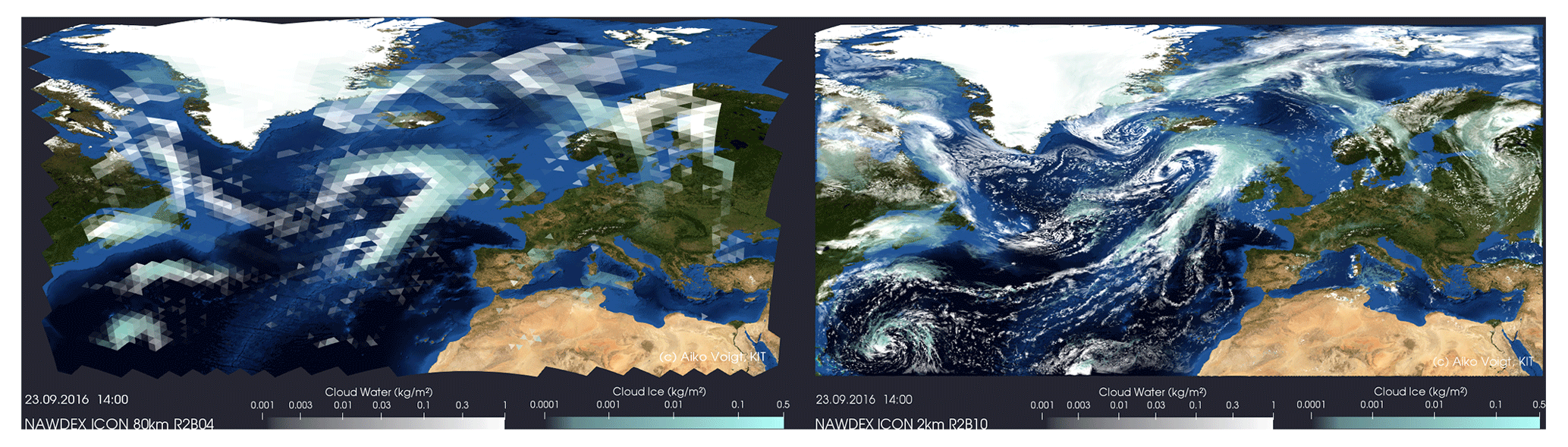
Figure 1 Illustrations of clouds simulated by a low-resolution version of the ICON atmosphere model with 80 km horizontal grid spacing (left) and a high-resolution version with 2 km horizontal grid spacing (right). The triangular grid structure is visible in the left panel.

The purpose of this paper is threefold. In Sect. 2, we first introduce the basic idea of our method and rigorously define its mathematical foundation. Secondly, given that the method has been practically implemented and an open-source Python package named TriCCo has been developed, we describe the implementation of the method in Sect. 3 and present an example of its application. The third purpose is to characterize the strengths and weaknesses of TriCCo's current implementation in Sect. 4, so as to both demonstrate its feasibility and point out how its computational performance can be improved. To this end, we also compare TriCCo to alternative approaches based on breadth-first search and graphs in Sect. 5. We discuss possible extensions of TriCCo and draw conclusions in Sect. 6. Readers who are mostly interested in the use of TriCCo might focus on Sects. 2.1 and 3 and 4.

2 Methodology: component labeling via cubulation

2.1 General idea

Before detailing the mathematical aspects of our method, we describe its general idea in this subsection. The method is based on the realization that a triangular grid can be embedded into a three-dimensional cubical grid. In the triangular grid, the cell centers are indexed as a one-dimensional array that, on its own, does not describe the neighbor relationships. In the cubical grid, in contrast, the triangles are indexed in terms of triples $(x,y,z)$, and the neighbor relations become self-evident.

The simultaneous, adjacency-preserving translation of cell indices in the triangular grid into $(x,y,z)$ positions in the cubical grid is called cubulation. This method makes use of the three sets of parallel classes of lines (also called hyperplanes) in the grid that are formed by the edges of the triangles. Each set of parallel lines is consecutively numbered and the position of a triangle can be described by the three indices of the lines that contain the triangle's edges. This process leads to the cubical coordinates.

Figure 2 Illustration of the general idea of the cubulation method. The triangular grid is shown in terms of the triangle edges in black. Some parallel hyperplanes are shown in the same colors.

The concept is illustrated in Fig. 2. The edges of the triangle cells are shown in black, and the base triangle is highlighted in cyan. Each edge of the base triangle is contained in a unique line in the plane. The three lines obtained in this way are highlighted in red, green, and blue. Each other line is parallel to one of the three lines. We enumerate these classes from 1 (green) to 3 (blue). Some examples of parallel lines are highlighted in the respective colors. As shown in Fig. 2, we index each line by a number, starting with the index 0 for the line containing the edge of the cyan triangle. The position of any triangle in the grid is described by means of the line indices of the hyperplanes. For example, the position of the highlighted triangle is $(\mathrm{0},\mathrm{0},\mathrm{0})$. The three neighbors that share an edge with the highlighted triangle have indices of $(\mathrm{1},\mathrm{0},\mathrm{0})$ (lower-left triangle), $(\mathrm{0},\mathrm{1},\mathrm{0})$ (lower-right triangle), and $(\mathrm{0},\mathrm{0},\mathrm{1})$ (upper triangle). For a precise description, see Definition 2.5.

As a result, the neighbors of a triangle are self-evident when the cubical positions are used, and the connected component labeling can be performed on a structured cubical grid.

2.2 Mathematics of the cubulation method

In this subsection, we describe the algorithm that transforms (a connected subset of) the regular triangle tiling of the Euclidean plane into a subset of the standard subdivision of ℝ³ into unit cubes. The method is a concrete example and implementation of Sageev's cubulation method introduced in Sageev (1995) for the Coxeter group of type ${\stackrel{\mathrm{̃}}{A}}_{\mathrm{2}}$. The vertices of this cubulation will have integer-valued coordinates. We start with some characteristics concerning the structure of the triangular grid in Sect. 2.2.1, collect some necessary background on cube complexes in Sect. 2.2.2, and then carry out the construction in Sect. 2.2.3

2.2.1 Structure of the triangle tiling

The cubulation of the regular triangle tiling of the plane is the key tool that makes TriCCo work. The regular triangle tiling of the plane will be called Σ in the following. The space Σ carries the structure of a (metrized) simplicial complex whose maximal simplices are all two-dimensional and in which all edges have the same length. A picture of this complex is provided in Fig. 3 below. The two-dimensional simplices are the triangles in this figure; edges are shown in black.

The cubulation that we construct may be restricted to any (connected) subset of the triangles of the plane and hence automatically yields a method to cubulate local lattices of any granularity.

There are three parallel classes of lines in Σ. We have illustrated these classes in Fig. 2 by highlighting some lines of the same class in the same color. These three classes will correspond to the three pairwise perpendicular coordinate axes of ℝ³ in which the cubulation lives.

We will now define a graph associated with Σ.

Definition 2.1.

The dual graph Γ_Σ of the triangle tiling Σ of the plane is defined as follows. The set of vertices V in Γ_Σ is the set of triangles in Σ. There is an edge (u,v) between $u,v\in V$ if and only if the triangles u and v share a codimension-one face, i.e., they have an edge in common.

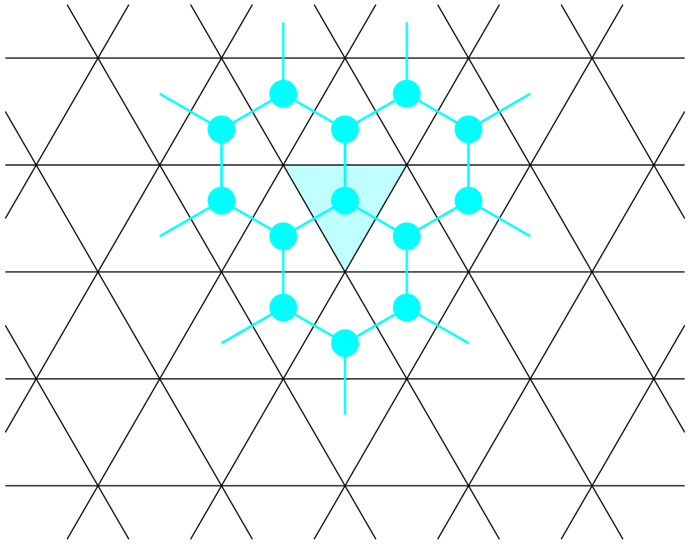
Figure 3 The figure shows a piece of the equilateral triangle tiling Σ of the plane. The turquoise vertices and edges represent the dual graph of the tiling as defined in Definition 2.1.

The dual graph can be pictured inside the tiled plane as follows. Draw a point in the center of each of the triangles. Each of these points represents a vertex of the graph Γ_Σ. Two points are connected by an edge whenever the corresponding triangles have a side in common. These edges may be drawn perpendicular to the common face. Figure 3 illustrates this correspondence.

Each vertex of the dual graph Γ_Σ by construction corresponds to a unique triangle in Σ. Every hexagon in Γ_Σ corresponds to a collection of six triangles in Σ sharing a common vertex.

2.2.2 Cubical complexes

Cubical complexes are spaces obtained by gluing unit cubes of various dimensions along isometric faces, i.e., faces of the same dimension. A unit cube is a cube that is in some Euclidean space of dimension k and has edges that are all of length 1. More formally, and in short, a cubical complex K is an M_k-polyhedral complex such that all the shapes are unit cubes, i.e., of the form [0,1]^k for some k∈ℕ. For more details on M_k complexes, see Bridson and Haefliger (1999) or Schwer (2019).

We will provide an ad hoc definition of a cubical complex below in order to allow the subject to be treated without the need to introduce general M_k-polyhedral complexes.

Definition 2.2 (cubes).

An n-cube is a set C of the form $C=[\mathrm{0},\mathrm{1}{]}^n\subset {\mathbb{R}}^n$. A codimension-one face of C is given by $F_{i,\mathit{ϵ}}:=\mathit{\{}x\in C\mathrm{|}{x}_i=\mathit{ϵ}\mathit{\}}$ for $\mathit{ϵ}\in \mathit{\{}\mathrm{0},\mathrm{1}\mathit{\}},i=\mathrm{1},\mathrm{\dots },n$. All other (proper) faces of C are non-empty intersections of codimension-one faces. We say that x∈C is an inner point of C if x is not contained in any (proper) face of C.

These cubes will now be glued together to form larger complexes. For technical reasons we will assume that the intersection of two cells in a cubical complex is either empty or a face of both. Some, but not all, of the gluings that do not satisfy this assumption can be resolved by further subdividing the complex into smaller cubes.

Definition 2.3 (cubical complexes).

Let C and C^′ be two cubes with faces F⊆C and $F^{\prime }\subseteq C^{\prime }$ ¹. A gluing of C and C^′ is an isometry $\mathit{\varphi }:F\to F^{\prime }$, which provides an identification of two of the sides of the cubes.

Suppose that 𝒞 is a set of cubes and 𝒮 a family of gluings of elements of 𝒞; that is, for all C∈𝒞, there is n_C∈ℕ such that $C\cong [\mathrm{0},\mathrm{1}{]}^{n_C}$ and every ϕ∈𝒮 is an isometry $\mathit{\varphi }:F\to F^{\prime }$ where $F,F^{\prime }$ are faces of cubes $C,C^{\prime }\in \mathcal{C}$. Assume further that (𝒞,𝒮) satisfies the following two conditions:

1. No cube is glued to itself.

2. For all $C,C^{\prime }\in \mathcal{C}$, there is at most one gluing of C and C^′.

Then (𝒞,𝒮) defines a cubical complex (X,d) by putting $X:=\left({\bigsqcup }_{C\in \mathcal{C}}C\right){/}_{\sim }$, where ∼ is the equivalence relation generated by putting x∼ϕ(x) for ϕ∈𝒮 and x∈dom(ϕ). The metric d on X is the length metric induced by the restricted Euclidean metric on each cube in 𝒞.

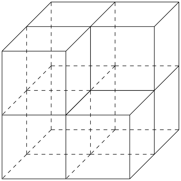
An example of a cubical complex is shown in Fig. 4.

One property of a cubical complex X is that the restriction of the quotient map $\mathrm{p}:{\bigsqcup }_{C\in \mathcal{C}}C\to X$ to one cube C∈𝒞 is injective. Also, the intersection of two cubes in X is either empty or a face of both (here, a face might be the whole cube). Hence, we may identify a cube C∈𝒞 with its image in C and write C∈X.

Figure 4 A cubical complex built out of seven 3-cubes.

One of the key features of a cubical complex is hyperplanes. Hyperplanes are cubical complexes themselves. They are by definition associated with the midcubes parallel to codimension-one faces of certain cubes. These hyperplanes then cut through the middles of adjacent cubes. Examples are shown in Fig. 5.

In a cube complex that satisfies the additional curvature property of being CAT(0), every hyperplane cuts the complex into two disjoint pieces called halfspaces. The partially ordered set of all these halfspaces allows the recovery of the cubical complex itself.

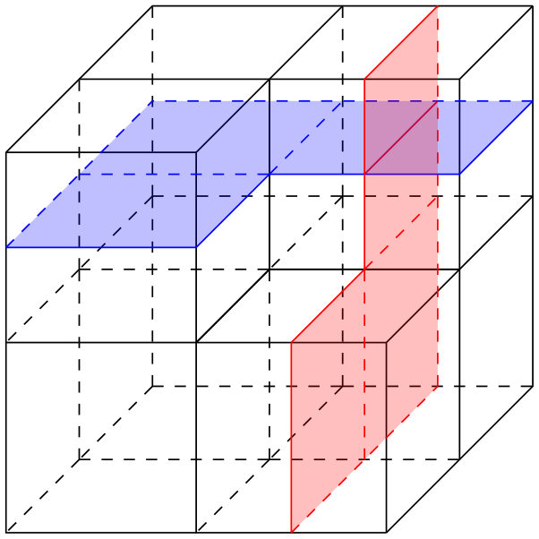
Figure 5 The blue and red two-dimensional cubical complexes are examples of hyperplanes in the cubical complex we have already seen in Fig. 4.

In the next section, we will cubulate the equilateral triangle tiling of the plane using the hyperplanes and halfspaces that appear in the tiling. More generally, one can introduce an abstract notion of halfspace systems and use those to cubulate more abstract spaces than the example we are considering here; see, for example, Schwer (2019).

Our main goal is the following.

Main goal.

Construct from every edge-connected subcomplex A of Σ a subcomplex X(A) of the standard cubulation X of ℝ³. The adjacency of triangles in the plane should be equivalent to the adjacency of the associated cubes in X.

As mentioned above, Euclidean 3-space can be subdivided and equipped with the structure of a (metric) cubical complex. We call this cube complex the standard cubulation of ℝ³ and denote it by X. Its vertices are the points in ℝ³ whose coordinates are all integers with respect to the standard basis $\mathit{\left\{}\right(\mathrm{1},\mathrm{0},\mathrm{0}),(\mathrm{0},\mathrm{1},\mathrm{0}),(\mathrm{0},\mathrm{0},\mathrm{1}\left)\mathit{\right\}}$. Denote this set of vertices by X⁽⁰⁾. Each cube edge is the interval between a pair of these integer-valued vertices that differ in exactly one entry. The graph that is formed by these vertices and edges is called the one-skeleton of X and is denoted by X⁽¹⁾.

2.2.3 Construction of the cubulation of Σ

In fact, we will not cubulate Σ but its dual graph Γ_Σ. To be precise, the goal is to define a simplicial map from Γ_Σ to the one-skeleton X⁽¹⁾ of the standard cubulation X of ℝ³.

We now introduce a labeling of the lines in the tiling Σ which will allow us to define such a map.

Definition 2.4 (labeling of hyperplanes).

A consistent labeling of the set of hyperplanes in Σ is achieved by the following procedure that assigns to every line the number of its class and an integer index as follows. Fix a base triangle v₀ in Σ. There exist then three hyperplanes, each containing one of the three sides of v₀. Call them $H_{\mathrm{1},\mathrm{0}},H_{\mathrm{2},\mathrm{0}}$, and H_3,0, respectively. In addition, there is a unique hyperplane parallel to H_i,0 whose intersection with v₀ is a single vertex. Call this hyperplane $H_{i,-\mathrm{1}}$ and enumerate all other hyperplanes in the same parallel class periodically.

See Fig. 2 for an illustration of the labeling we have just defined. In the next definition, we obtain coordinates for the vertices in Γ_Σ from the labeling defined in Definition 2.4. These can be used to define a map from the vertex set V of Γ_Σ to the vertices X⁽⁰⁾⊂X.

Definition 2.5 (the 3-D coordinates for triangles).

Recall that V is the set of vertices of the dual graph Γ_Σ. For each v∈V, define three-dimensional coordinates $(v_{\mathrm{1}},v_{\mathrm{2}},v_{\mathrm{3}})$ by putting v_i:=k if the triangle in Σ corresponding to v lies between the hyperplanes H_i,k and $H_{i,k-\mathrm{1}}$ in Σ.

In Fig. 3, the dual graph Γ_Σ is shown in turquoise. The vertex of the dual graph inside the turquoise triangle has coordinates $(\mathrm{0},\mathrm{0},\mathrm{0})$. Vertices contained in a common hexagon of the dual graph will be mapped to the same 3-cube in the cubulation.

Definition 2.6 (cubulation map).

The cubulation map $f:V\to X^{\left(\mathrm{0}\right)}$ is defined by $v\mapsto (v_{\mathrm{1}},v_{\mathrm{2}},v_{\mathrm{3}})$, where the v_i are chosen as in Definition 2.5.

Figure 6 illustrates some of the images of vertices in Γ_Σ inside the 1-skeleton of X.

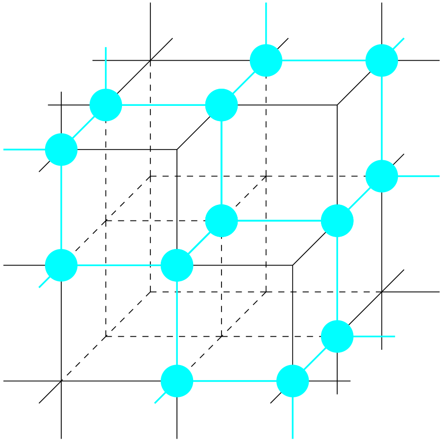
Figure 6 Illustration of the mapping from Γ_Σ to X⁽¹⁾ showing how the dual graph sits inside the three-dimensional cubical complex.

The cubulation map satisfies some properties and, in particular, preserves adjacency of vertices.

Proposition 2.7 (properties of the cubulation map).

Let f be the map defined in Definition 2.6. Then the following holds:

1. The map f preserves adjacency; that is, the coordinates of two adjacent vertices u,v in Γ_Σ differ in exactly one entry. Their images in X⁽¹⁾ under f are connected by an edge.

2. Every hexagon in Γ_Σ is mapped into a unique cube of X.

3. Triangles u,v that share a vertex in Σ are mapped to vertices that are contained in the same cube.

Proof.

To see the first item, let u, v be adjacent vertices in Γ_Σ. They then correspond to two triangles that share a common side. This side is contained in a unique hyperplane H_i,k for some parallel class i and some index k. Therefore, the coordinates v_i and u_i differ by one. If there was a second coordinate in which u and v differ, there would be a second hyperplane in a different parallel class separating u and v, but this is impossible.

By checking one of the hexagons by hand, one can verify that the second property is satisfied and all vertices of this hexagon are mapped to a common cube. The vertices in all other hexagons have hyperplane coordinates shifted by integer values in at least one of the three directions obtained from the parallel classes of hyperplanes. This yields the assertion.

The third item follows from the second by checking that triangles sharing a vertex are contained in a common hexagon in Γ_Σ.

We can characterize the full image of f and describe which points in X⁽¹⁾ are part of the embedded graph Γ_Σ.

Proposition 2.8.

The image f(V) of all the vertices in Γ_Σ is the collection of points in X⁽¹⁾ whose coordinates sum to either 1 or 0. Each edge (u,v) has a vertex with coordinates that sum to 0 and one with coordinates that sum to 1.

Proof.

Let u and v be two triangles sharing an edge. For each i, there is an index k_i such that u lies between $H_{i,k_i}$ and $H_{i,k_i-\mathrm{1}}$ and u has coordinates $(k_{\mathrm{1}},k_{\mathrm{2}},k_{\mathrm{3}})$. Observe that v lies between the same two parallel hyperplanes for two of the indices. Moreover, there is one index, say j, for which v is either between $H_{j,k_j+\mathrm{1}}$ and $H_{j,k_j}$ or between the two hyperplanes $H_{j,k_j-\mathrm{1}}$ and $H_{j,k_j-\mathrm{2}}$.

Without loss of generality, let j=1. Suppose first that v is between $H_{\mathrm{1},k_{\mathrm{1}}}$ and $H_{\mathrm{1},k_{\mathrm{1}}+\mathrm{1}}$. Then v has coordinates $(k_{\mathrm{1}}+\mathrm{1},k_{\mathrm{2}},k_{\mathrm{3}})$ and the coordinate sum differs by 1. In the case where v is between $H_{\mathrm{1},k_{\mathrm{1}}-\mathrm{1}}$ and $H_{\mathrm{1},k_{\mathrm{1}}-\mathrm{2}}$, it has coordinates $(k_{\mathrm{1}}-\mathrm{1},k_{\mathrm{2}},k_{\mathrm{3}})$ and the coordinate sum differs by −1.

It is still necessary to prove that coordinate sums alternate between 0 and 1. The base triangle v₀ has coordinates $(\mathrm{0},\mathrm{0},\mathrm{0})$ and hence a coordinate sum of 0. Its neighbors lie, by construction, between hyperplanes with indices 0 and 1 in one of the three directions and hence have a coordinate sum of 1.

One can proceed by induction on the distance to v₀ in Γ_Σ and prove that along any shortest path in Γ_Σ connecting an arbitrary vertex to v₀, the coordinate sums alternate between 0 and 1.

2.3 Identifying connected components for 2-D data

After having computed the cubulation of the triangular grid, we can use it to detect connected components.

There are two ways to define connectivity on a triangular grid: either via shared edges (edge connectivity) or via shared vertices (vertex connectivity). The two types of connectivity can also be defined more rigorously as follows. A subset of the triangles of the triangle tiling Σ is edge connected if, for any two triangles, the corresponding vertices in the dual graph are connected by a path in the dual graph. We say that a set A of triangles is vertex connected if, for every pair of triangles u and v in A, there exists a sequence of triangles $v_i\in A,i=\mathrm{0},\mathrm{\dots },n$ connecting u and v such that two subsequent triangles v_i and v_i+1 share a vertex.

We need to to clarify how connectivity for cells on the triangular grid translates to connectivity for the cubical grid. One can show that edge connectivity on the triangular grid corresponds to face connectivity (also known as 6-connectivity) on the cubical grid and that vertex connectivity on the triangular grid translates precisely to vertex connectivity (also known as 26-connectivity) on the cubical grid.

2.4 Identifying connected components of 3-D data

We now describe how connectivity is computed for three-dimensional data. An example of three-dimensional data is the cloud fraction. Cloud fraction depends on the horizontal (i.e., geographical position), which is described by the triangular grid, and the altitude. To represent the vertical dimension, the ICON model stacks layers of horizontal grids. This treatment of the vertical dimension is standard in atmospheric modeling.

We understand connectivity in the vertical dimension to mean that neighboring layers share at least one triangle in the horizontal grid. For example, if a cell i corresponding to latitude–longitude position (φ,λ) has the same value at model level k and the model level below, k+1, then the grid volumes spanned by (k,i) and $(k+\mathrm{1},i)$ are connected. We note that we thus limit connectivity in the vertical to cell faces. This is consistent with the typical treatment of vertical exchange in atmospheric models, which occurs columnwise apart from in a few exceptions such as three-dimensional radiative transfer.

With this, connected components in 3-D can be computed from a three-step procedure. In a first step, 2-D components are identified for each model level separately following the method described in Sect. 2.3. Each 2-D component is considered a node of an undirected graph. In a second step, we identify all pairs of 2-D components that reside in neighboring model levels and share at least one triangle. The pairs are edges between the nodes formed by the 2-D components. In a third step, we apply a connected component analysis on these nodes and edges formed by the set of 2-D connected components. The overall result of this procedure is a list of 3-D connected components, where each 3-D connected component is given by a list of 2-D connected components. For the connected component analysis of step three, we use the external library NetworkX implemented in Python (Hagberg et al., 2008), but our procedure would also work for other external network analysis libraries.

3 Software implementation and application examples

In this section, we describe the software implementation and provide basic examples of how to apply the method to cloud fields simulated by the ICON atmosphere model. Our aim is to provide an orientation on the code structure and its usage. Version 1.1.0 of the implementation described and used here is available via gitlab and pypi, and is long-term archived at zenodo (see “Code availablility”; Voigt, 2022).

The implementation of TriCCo and its use consist of four steps. Each step is described in the following. Note that the terms “triangle” and “cells” are used interchangeably with no risk of confusion as our method is designed for triangular cells.

3.1 Step 1: Preparing the horizontal grid

Regarding the horizontal triangular grid, information on the neighboring cells and the edges of each cell is needed, as well as information on the vertices that form a specific edge. The grid information is stored in an xarray dataset (Hoyer and Hamman, 2017) named grid, using variable names that follow the convention of the ICON model grid. This variable naming is used due to the fact that the ICON grid was used during the development and testing of code. The code includes routines specific to the ICON grid. It should be straightforward to adapt the routine to other grids.

Let us assume that the grid consists of n_c cells, n_v vertices, and n_e edges. For a triangular grid that covers the entire sphere, n_v and n_e are given by n_c, as described in Zängl et al. (2015); for a limited-area grid, the relationships hold in an approximate manner. The three variables required to describe the grid are as follows:

• neighbor_cell_index defines the three neighboring cells for each cell. The dimension is (3,n_c).

• edge_of_cell defines the three edges for each cell. The dimension is (3,n_c).

• edge_vertices defines the two vertices for each edge. The dimension is (2,n_e).

The variables are indexed starting from 0. In ICON, this requires a shift by −1 as the indexing starts with 1. The variables are accessed by three analogously named functions that provide the variable values for a single grid cell or edge. For a limited-area grid, a missing neighboring cell indicates the grid boundary and is assigned a value of −9999.

3.2 Step 2: Computing the cubulation of the horizontal grid

The main function is compute_cubulation. This function implements the cubulation described in Sect. 2 and computes, for each grid cell i, the associated 3-D coordinate on the cubical grid $(x,y,z)$. This information defines the cubulation and is stored in cube_coordinates as a list of arrays of the form $(i;(x,y,z\left)\right)$.

The function compute_cubulation starts at a user-specified start_triangle, and iteratively computes all cube coordinates within an expanding circle around the start cell. The iteration stops when the circle reaches a user-specified radius. The radius needs to be chosen according to the grid size, or can alternatively be set to a smaller value if only a specific part of the grid is of interest. If the radius is too small, the cubulation will not cover the entire grid. On the other hand, if the radius is too large, the algorithm will iterate over empty lists for the last steps. Setting print_progress=True outputs the progress of the iteration to screen, allowing one to monitor the number of new cells added in each round, which is helpful for choosing the radius. Also, even though iterating over empty lists comes with essentially no computational burden, the size of the cubulation increases with the radius, which in turn increases the memory demand of the connectivity analysis in Step 4. The radius should thus be as small as possible.

The following consideration is helpful when choosing the radius r. Each iteration adds 3⋅i cells, where i≤r is the number of the current iteration. The total number of visited cells is

$$\begin{array}{}\text{(1)}& n_{\mathrm{c}}=\mathrm{1}+\sum _{i=\mathrm{1}}^r\mathrm{3}\cdot i=\mathrm{1}+\mathrm{3}\cdot {\displaystyle \frac{r(r+\mathrm{1})}{\mathrm{2}}}=\mathrm{1}+\mathrm{1.5}r+\mathrm{1.5}{r}^{\mathrm{2}}.\end{array}$$

The sum begins with 1 due to the start cell. Thus, covering n_c cells requires a search radius of

$$\begin{array}{}\text{(2)}& r=-{\displaystyle \frac{\mathrm{1}}{\mathrm{2}}}+\sqrt{{\displaystyle \frac{\mathrm{1}}{\mathrm{4}}}+{\displaystyle \frac{\mathrm{2}}{\mathrm{3}}}(n_{\mathrm{c}}-\mathrm{1})}.\end{array}$$

The equation is exact as long as the iteration has not reached the grid borders, i.e., it works best for circle-shaped grids such as those used by Schemann and Ebell (2020). For other grids, the equation serves as a lower bound of the radius that one needs to cover n_c cells. Acknowledging that n_c≫1, the lower bound can effectively be approximated by $r\mathit{⪆}\sqrt{\frac{\mathrm{2}}{\mathrm{3}}{n}_{\mathrm{c}}}$.

Another helpful approach to finding the search radius is to start from a value somewhat larger than the lower bound and adapt the radius based on the diagnostic output of compute_cubulation, which can be obtained by print_progress=True.

A few aspects of compute_cubulation warrant further description. The function begins by assigning the cube coordinates $(x,y,z)=(\mathrm{0},\mathrm{0},\mathrm{0})$ to start_triangle, but these are not the final coordinates of the start cell, as explained further below. In each iteration, all “new” cells that are adjacent to already visited cells are considered and their cube coordinates are calculated. Missing neighbors, which occur for cells at the border of the grid, are identified by −9999 and ignored (see Sect. 3.1).

Moreover, the edges of a new cell need to be colored, and this needs to be done such that the edge colors are consistent with the edge colors of other cells; i.e., parallel edges need to have the same color, as they belong to the same hyperplane. This is illustrated for two neighboring cells in Fig. 7, where the left cell is old and the right cell is a yet-to-be-visited neighbor, new. The joint edge is already colored, as old was visited in the preceding iteration. This leaves the task of coloring the two non-joint edges of new. If only one edge is uncolored, its color is given by the color which has not yet been used. If two edges of new need to be colored, their colors are deduced from the edge colors of old: a non-joint edge of new has the same color as a non-joint edge of old if both edges share no vertices and hence are parallel.

The cube coordinates are computed in the following manner. As old and new are adjacent, their cube coordinates differ by ±1 in exactly one entry of $(x,y,z)$ by Proposition 2.9. The color of the joint edge between the two cells defines which entry needs to be changed. Whether the entry differs by +1 or −1 follows from the constraint that the sum of cube coordinates, $x+y+z$, must be either 0 or 1 (see Proposition 2.9); that is,

$$\begin{array}{c}{\displaystyle }\text{old}\text{has a coordinate sum of}\mathrm{0}\Rightarrow \mathtt{\text{new}}\text{has a coordinate sum of}\mathrm{1}\\ {\displaystyle }\text{old}\text{has a coordinate sum of}\mathrm{1}\Rightarrow \mathtt{\text{new}}\text{has a coordinate sum of}\mathrm{0}.\end{array}$$

After all cells have been visited and the iteration is finished, the cube coordinates are shifted by radius/2 (rounded down to an integer value) for all three dimensions to ensure that all coordinates are positive.

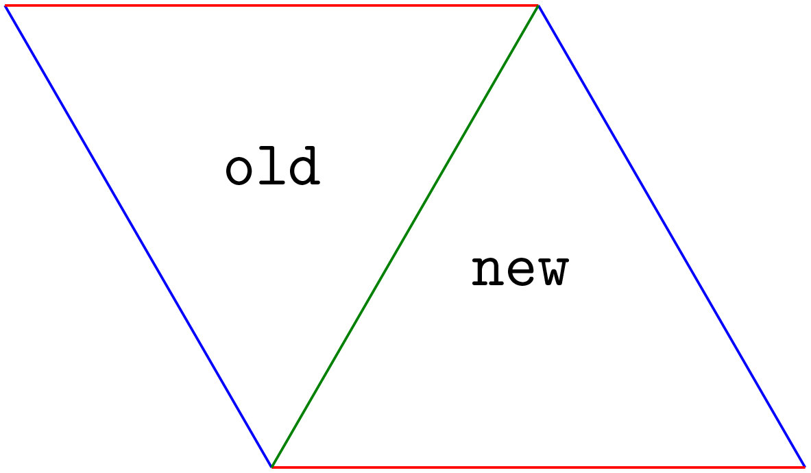
Figure 7 Illustration of how to color the edges of a newly visited cell (right) based on the edge colors of an old cell (left).

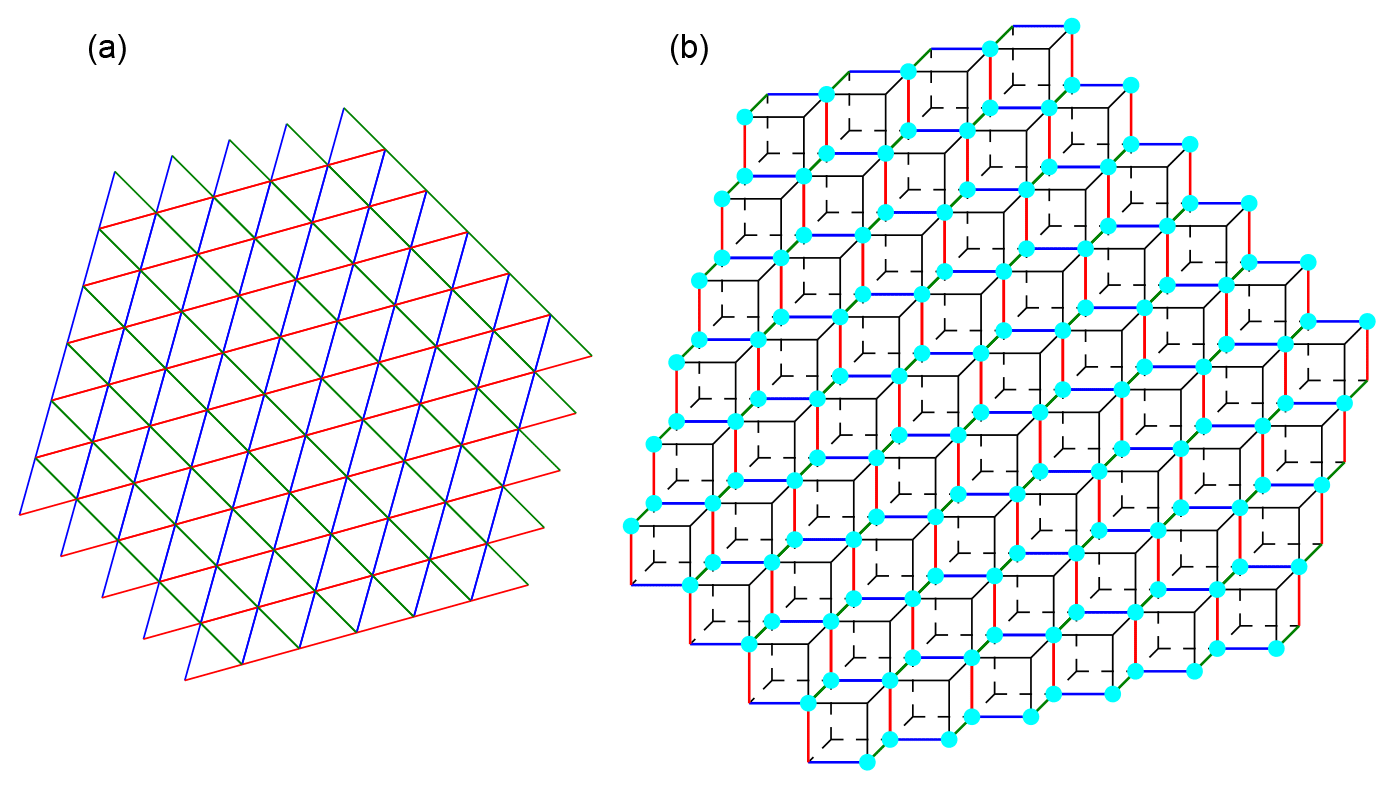
Figure 8 Illustration of compute_cubulation. The triangular grid is shown in (a) and the corresponding cubical grid in (b). In (b), cyan vertices correspond to triangle centers in (a), and analogously for colored edges. Vertices with no colors in (b) do not correspond to triangle centers.

3.3 Step 3: Preparing the simulation data

The simulation data need to be moved from the triangular grid to the cube coordinates of the cubulation. This is achieved by the function prepare_field for single-level data and by the function prepare_field_lev for multi-level data. The functions are wrappers for model-specific functions. We include such functions for the ICON model; writing analogous functions for other models and their data format should be straightforward.

prepare_field and prepare_field_lev require as input the cubulation computed in Step 2 and a threshold value. The latter is used to convert the input data to values of either 0 or 1, depending on whether the input data are smaller than than the threshold or equal to or larger than the threshold. The functions return the thresholded input data on the triangular grid as well as on the cubical grid, where the data on the cubical grid have dimensions of (radius +1)³ for single-level data and nlev × (radius +1)³ for multi-level data, with nlev being the number of levels. In the case of multi-level data, the first entry corresponds to the model level and the following entry describes the horizontal position. For the triangular grid, the horizontal position is given by the cell index i; for the cubical grid, it is given by the three integers $(x,y,z)$.

prepare_field_lev moves the entire multi-level data to the cubical grid, which, for larger grids, can result in a large memory burden (see Sect. 4). The memory burden can be easily reduced by working separately on each level by means of prepare_field and using the function compute_levelmerging to connect components in the vertical. An example of how this is achieved is provided in the juypter notebook example-3d.ipynb.

3.4 Step 4: Computing connected components

Once the cubulation is known and the simulation data are prepared, the connected components are computed by the functions compute_connected_components_2d and compute_connected_components_3d, respectively. The functions require as input the cubulation (Step 2) and the prepared simulation data on the cube grid (Step 3).

Two types of connectivity in the horizontal direction can be chosen: vertex or edge connectivity. For edge connectivity, cells in the horizontal belong to the same component if they share a triangle edge. For vertex connectivity, they also belong to the same component if they share only a triangle vertex. Vertex connectivity thus results in larger but fewer connected components. The default choice is vertex connectivity. Examples illustrating edge and vertex connectivity are provided in Figs. 10 and 9.

The functions compute_connected_components_2d and compute_connected_components_3d use the external library cc3d (Silversmith, 2021) to identify connected components on a single model level. cc3d can identify connected components in three dimensions for 26- and 6-connectivity, and uses a 3-D variant of the two-pass method by Rosenfeld and Pfaltz (1966) augmented with union-find and a decision tree based on Wu et al. (2005). For multi-level data, the external library NetworkX (Hagberg et al., 2008) is used to merge connected components in the vertical by constructing a corresponding graph (see Sect. 2.4) and applying breadth-first search. The final result of both functions is a list of connected components. For 2-D data, a connected component is given by a list of triangular cell indices. For 3-D data, it is given by a list of tuples, with each tuple consisting of the model level and cell index.

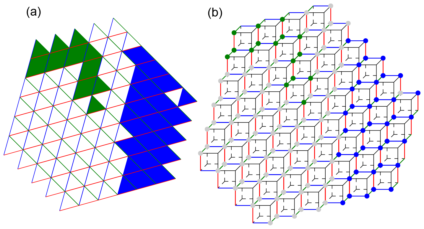
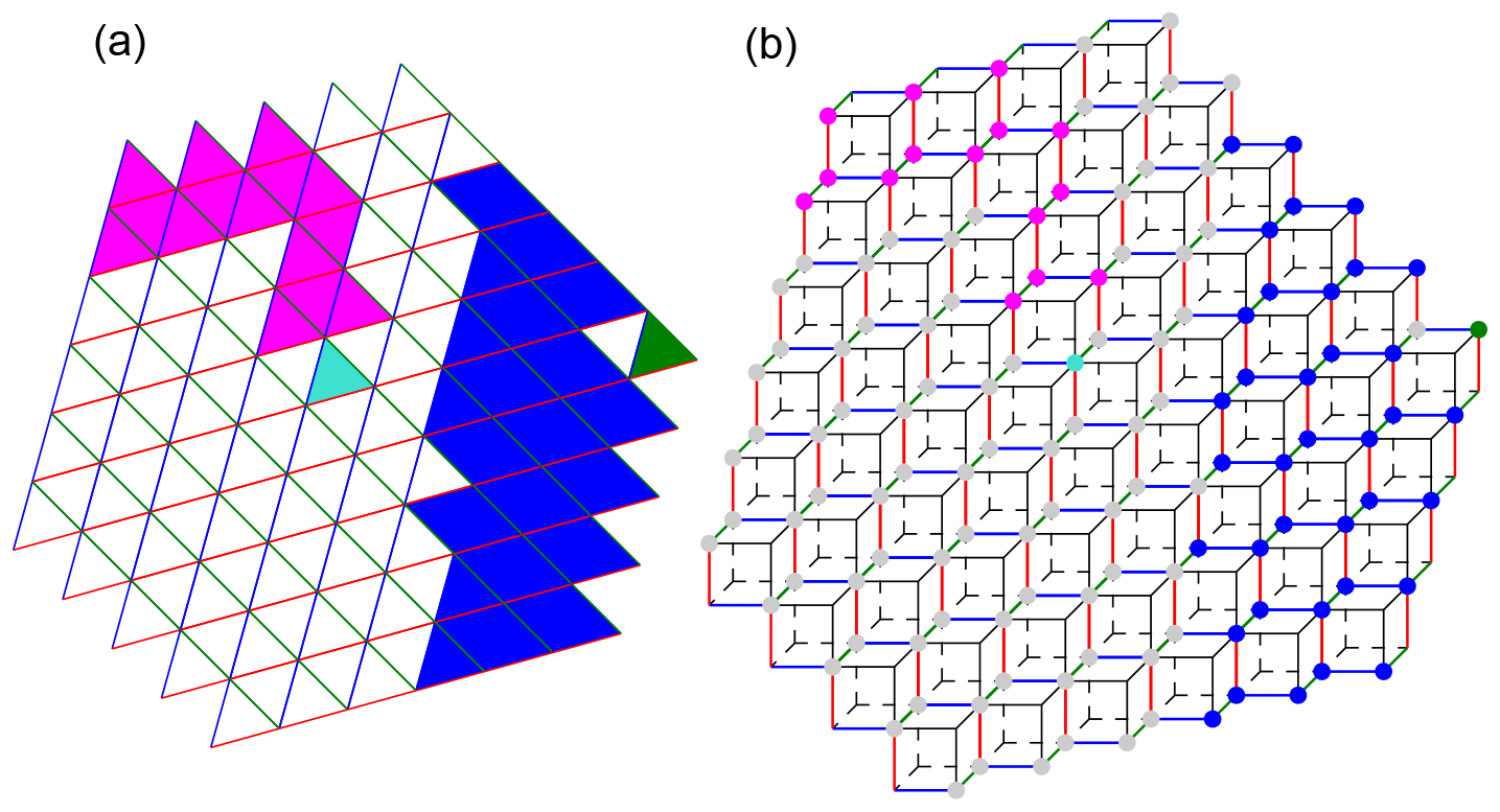
Figure 9 Illustration of the result of connected component labeling for 2-D data and vertex connectivity. In (a), connected components are formed by cells with the same face color. The colors of the cell edges that form the hyperplanes of the cubulation are also shown. Panel (b) illustrates the same data on the cubulation. Triangles in (a) correspond to vertices in (b). A set of triangles on the triangular grid is vertex connected if any two of the vertices on the cubical grid can be connected by a sequence of vertices where subsequent ones are in a common two-dimensional face (i.e., a square) of a cube.

Figure 10 Same as in Fig. 9 but for edge connectivity. A set of triangles on the triangular grid are edge connected if any two of the vertices on the cubical grid can be connected by a sequence of vertices such that two subsequent ones are connected by an edge of a cube.

3.5 Application examples

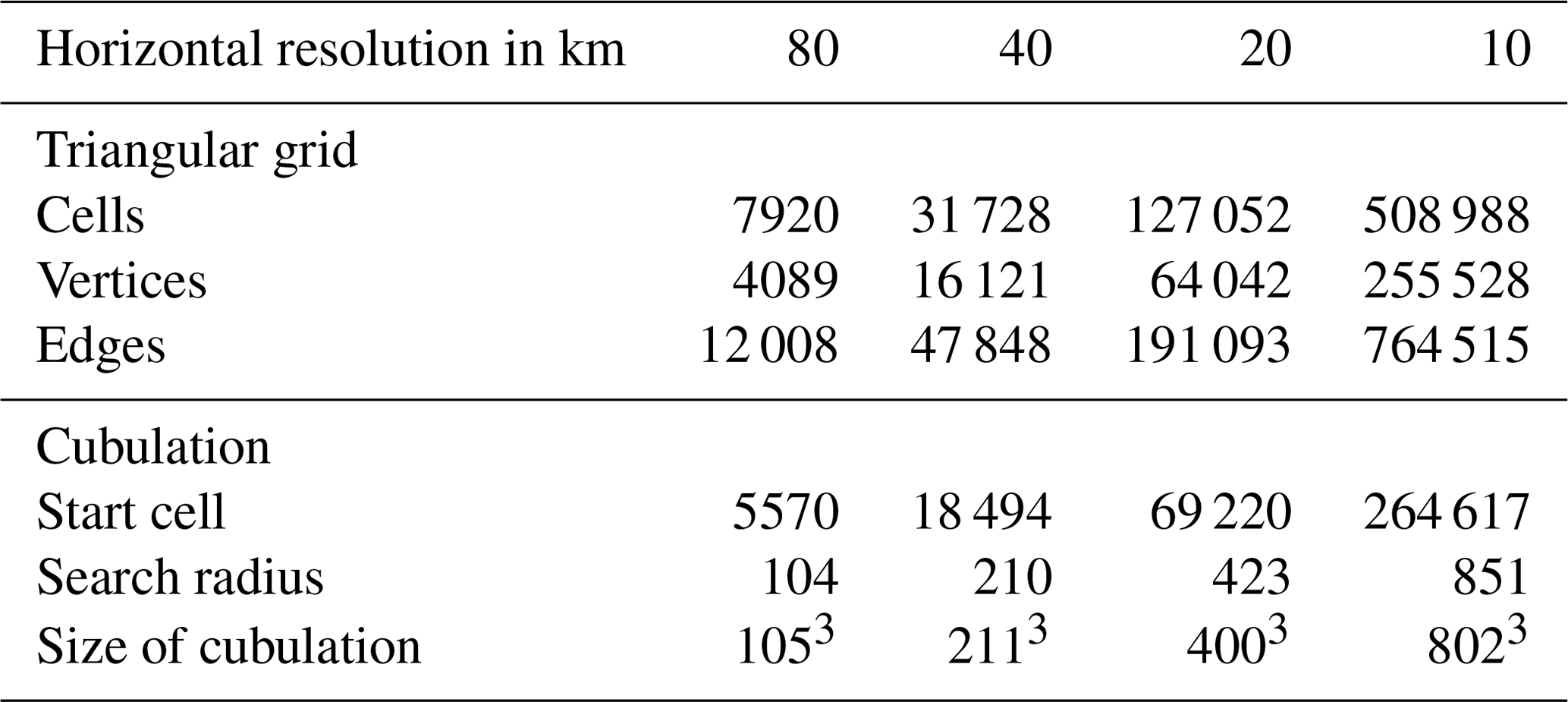
As an illustration of TriCCo's abilities, we analyze model output from the ICON atmosphere model in a limited-area setup over the North Atlantic. The output is from a simulation that applies a triangular grid with 7920 cells and 75 model levels and that is part of a larger set of simulations presented in Senf et al. (2020) and Stevens et al. (2020) from a scientific perspective. In our work here, the simulation output solely serves as technical input to test and illustrate the functionality and performance of the TriCCo routine. The grid has a nominal horizontal resolution of 80 km. Its characteristics are listed in Table 1. We use total cloud cover for demonstrating the use of data on a single model level, and the vertically resolved cloud fraction at 75 levels as an example for multi-level data.

The simulation domain is illustrated in Fig. 1 and extends from 78^∘ W to 40^∘ E, and from 23 to 80^∘ N, covering the North Atlantic, the Mediterranean, the larger part of Europe, and parts of Northern Africa. To find the start cell, we search for the cell with the smallest distance to the grid center at 19^∘ W and 51.5^∘ N, where we measure the distance in terms of the great circle distance on the sphere using the haversine formulae. We then find the radius by using the lower bound and the diagnostic output of compute_cubulation as described in Sect. 3.2. The start cell and radius are given in Table 1.

Figure 11 shows the result of connected component labeling for total cloud cover, which in ICON ranges between 0 % (cloud free) and 100 % (completely covered with cloud). Panel (a) shows the total cloud cover from a single time step of the simulation. Centered at roughly 20^∘ W and 50^∘ N, there is a comma-shaped cloud band that is associated with a warm conveyor belt of a North Atlantic extratropical cyclone. We threshold the data at 85 %, as shown in panel (b), and identify connected components for vertex (panel c) and edge (panel d) connectivity. For vertex connectivity, the comma-shaped cloud band is connected to a cloud structure west of it. Using edge connectivity instead, the cloud band can be isolated. Overall, vertex connectivity leads to 31 connected components, compared to 74 components when the stricter criterion of edge connectivity is used.

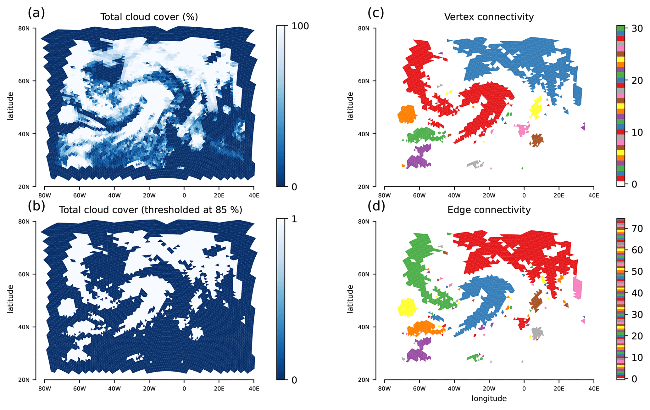
Figure 11 Application for total cloud cover from an ICON simulation with a limited-area grid over the North Atlantic. The triangular nature of the grid is visible. (a) Total cloud cover in percent, with 0 corresponding to cloud-free and 100 to completely overcast conditions. (b) Total cloud cover thresholded at 85 %, with values above 85 % set to 1 and values below set to 0. (c) Connected components for vertex connectivity, with components plotted in different colors. (d) Connected components for edge connectivity. In (c) and (d), the connected components are ordered according to their sizes, starting with the largest component.

We also present results for connected component labeling for the vertically dependent cloud fraction from the same time step, where we again apply a threshold of 85 %. For vertex connectivity, we identify 235 components, whereas edge connectivity results in 381 components. Figure 12 shows the component that corresponds to the comma-shaped cloud band centered at 20^∘ W and 50^∘ N. Note that for display purposes, the horizontal grid is rotated and latitude decreases from left to right. The vertical structure of the cloud band is clearly visible, as is the fact that vertex connectivity associates more cells with the connected component than edge connectivity does. This can be seen, for example, near the surface around 10^∘ W and 40^∘ N.

The Python code of the examples presented here is included in TriCCo as the jupyter notebooks examples-2d.ipynb and examples-3d.ipynb.

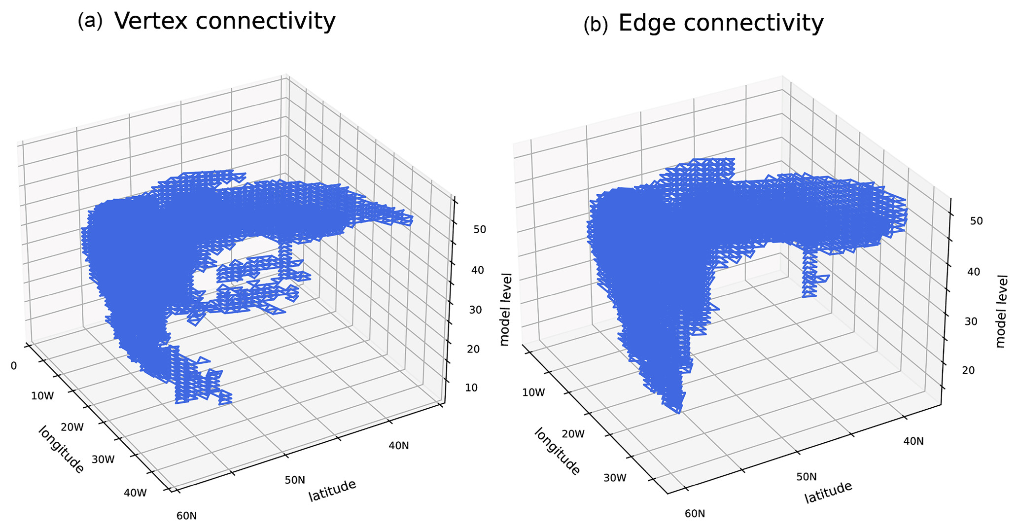
Figure 12 Application to vertically varying cloud cover from the ICON simulation also used in Fig. 11. The plot shows the connected component corresponding to the comma-shaped cloud band near 20^∘ W and 50^∘ N for vertex connectivity (a) and edge connectivity (b). The model levels are counted upward from the earth's surface, so that level 10 is near the surface and level 55 is in the upper troposphere.

4 Benchmarks and computational challenges

The ICON simulation analyzed in Sect. 3.5 is part of a larger set of simulations that includes triangular grids with much finer resolution. In this section, we use this larger set to characterize the computational aspects of TriCCo, and to identify limitations of the current implementation. The limitations result, for example, from the current serial implementation that restricts its use to a single core. Ultimately, they reflect that our expertise, as climate scientists and pure mathematicians, in software development and computational science is finite.

We use simulations with horizontal resolutions ranging from 80 to 10 km. Their grid specifics are included in Table 1. Because we are interested in the computational performance, what matters here is not the grid resolution itself but the number of grid cells. The latter increases by roughly a factor of 4 for each grid refinement. The start cells and search radii depend on the grid, and we find them by following the approach outlined in Sect. 3.5. The benchmarks are run on a single core of a dedicated compute node of the Levante HLRE-4 supercomputer of Deutsches Klimarechenzentrum in Hamburg, Germany, which became operational in spring 2022. The Levante compute node is equipped with two AMD 7763 EPYC CPUs (64 cores, base frequency of 2.45 GHz) and 256 GB of main memory (https://docs.dkrz.de/doc/levante/configuration.html, last access: 4 October 2022).

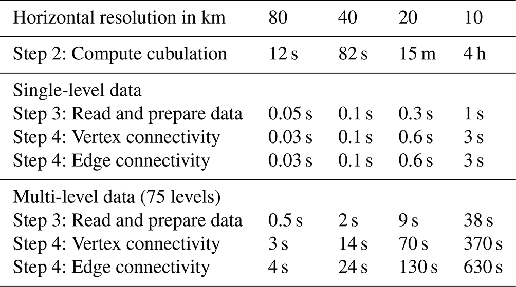
Table 1 Size of the triangular grids used for benchmarking, as well as characteristics of the associated cubulations.

We measure the time needed for Steps 2, 3, and 4 described in Sect. 3. The computational cost for Step 1 is virtually zero and not considered. As in Sect. 3.5, we use total cloud cover for single-level data and cloud fraction at 75 model levels for multi-level data.

The time required to compute the cubulation (Step 2) increases strongly with the number of grid cells (Table 2). For the coarsest grid with 80 km resolution and 7920 cells, the cubulation is computed within a few seconds; for the 10 km grid with 508 988 cells, this step takes 4 h. We find this result encouraging, as it shows that even our rather naive implementation can handle grids that contain up to 500 000 cells. To put that number into perspective, global simulations with ICON in climate mode are run using grids with 20 480 cells (R2B4 resolution; Giorgetta et al., 2018), and global simulations with ICON in weather-prediction mode for research purposes typically use grids with 327 680 cells (R2B6 resolution; Selz, 2019; Baumgart et al., 2019). Such grids are accessible already with our current implementation, despite a clear need for improvement if one aims to handle larger grids, including those used in global storm-resolving models (Satoh et al., 2019). However, it is also important to keep in mind that the cubulation needs to be computed only once for a given grid. Hence, the time for computing the cubulation itself is not a limiting factor for use cases with many time steps or simulations done on the same grid.

Table 2 also includes the times required for reading and preparing the simulation data (Step 3), and for computing connected components (Step 4). In real-world applications of TriCCo, both steps are done together. Here, their times are separated to help identify performance bottlenecks. The times are obtained from 10 repetitions of analyzing 48 output time steps and are given as the average time required for a single time step. An exception is the 10 km grid for multi-level data, for which the time is obtained from a single analysis of 10 time steps due to the rather large computational expense and the 8 h wall-clock limit for a batch job on Levante's compute partition. All times are given per single time step.

The time taken computing the connected components dominates when compared to the time taken reading and preparing the data. For single-level data, computing the connected components requires only a few seconds for the 10 km grid and (much) less than 1 s for the smaller-sized grids. This shows that the current implementation is feasible for single-level data. For multi-level data, the picture is mixed. The time stays within a few seconds for the 80 km grid but increases strongly as the grid size is increased. For the 10 km grid, analyzing a single time step takes up to 10 min. In practice, this may limit the application of TriCCo to grids of this size and larger.

Table 2 Times required for different aspects of TriCCo's Python implementation for different sizes of the triangular grid. The times are obtained from benchmarks on the DKRZ Levante supercomputing system.

Besides speed, another matter of concern is the amount of required main memory. In the current implementation, the entire data on the cubical grid needs to be held in memory. The size of this data increases with the size of the cubulation, which is included in the last line of Table 1. For example, the cubulation of the 10 km grid consists of ${\mathrm{802}}^{\mathrm{3}}=\mathrm{516}\times {\mathrm{10}}^{\mathrm{6}}$ cells, meaning that the cubulated version of single-model-level data requires approximately 500 MB of memory if one assumes that the data are stored as 1 byte integers. For multi-level data on, e.g., 75 levels, the requirement increases to 36 GB, although the memory requirement can be reduced to essentially that for single-level data by treating levels separately, as described in Sect. 3.4. Nevertheless, TriCCo's thirst for memory can become immense. While the memory requirement can be satisfied on high-performance computers (for example, a DKRZ Levante compute node has 256 GB of memory), this might pose a problem for the general applicability of TriCCo and for grids larger than those considered here.

The need to reduce the amount of required memory is also evident from a consideration of information density. In the triangular grid, each cell contains information, and the information density is maximum. When the data are moved onto the cubical grid, the vast majority of cells in fact do not correspond to a cell on the triangular grid and contain no information, i.e., the information density is very low. A striking example is the 10 km grid, for which, out of the 516 million cells of the cubical grid, only 508 988 correspond to a cell on the triangular grid; that is, less than 0.1 %. Put differently, the data moved to the cubical grid data comprise a very sparse matrix whose entries are overwhelmingly trivial zeros.

5 Comparison to alternative methods

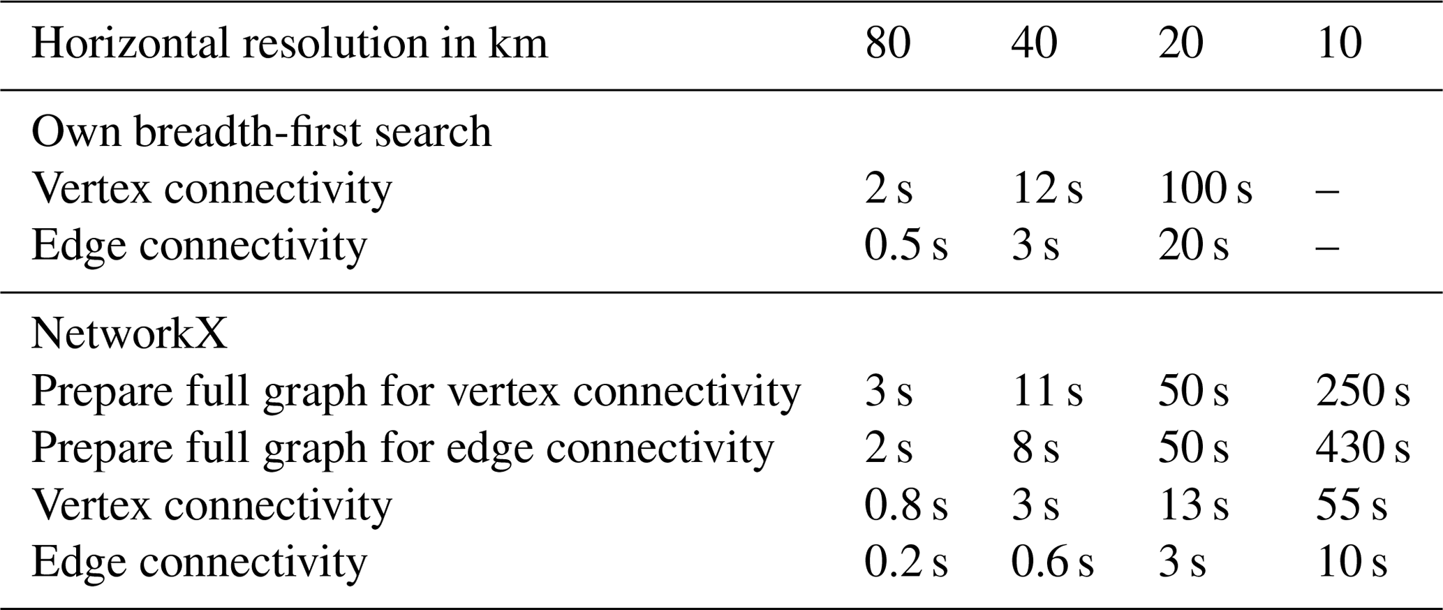
To put TriCCo's performance into context, we test two alternative methods. The first is breadth-first search, which we have implemented ourselves in Python. The second makes use of the NetworkX library, which provides functions to build a graph and search for its connected components via breadth-first search. Breadth-first search is a well-established, simple algorithm for searching a graph and is guaranteed to find all connected components (Cormen et al., 2009). The choice of the NetworkX library is pragmatic since we already use it in TriCCo for merging connected components in the vertical (see Sect. 3.4). Other graph libraries might be faster than NetworkX (Staudt et al., 2014), but our aim here is not to provide an exhaustive comparison of TriCCo to other methods and implementations, of which there are many (He et al., 2017). Rather, by choosing NetworkX, we emphasize the perspective of a TriCCo user that we have in mind: a geophysical modeler and data analyst with good experience in Python but little background in computer science and computer vision (e.g., the first author of this paper).

The two alternative methods are included in TriCCo's repository; their use is documented via the juypter notebooks alternative_own-bfs_2d.ipynb and alternative_networkx_2d.ipynb. We only consider single-level data. Performance differences for single-level data carry over to multi-level data in a straightforward manner because multi-level data are treated by looping over single-level data and then merging levels. As in Sect. 4, the two methods are benchmarked on the DKRZ Levante system, with the times reported in Table 3. For both methods, the time taken to read and prepare (i.e., threshold) the data is not listed as it remains below 0.1 s for all grids. The read and prepare step is faster compared to TriCCo, as the data remains on the triangular grid and does not need to be moved to the cubical grid.

Regarding our own breadth-first search, the timing is clearly disadvantageous compared to TriCCo (Table 3); e.g., for the 20 km grid, a single time step takes more than 1 min for vertex connectivity, which is more than 100 times slower than TriCCo. The approach, while simple and short in terms of programming, quickly becomes impractical as the grid becomes larger. As a result, we have not tested it for the grid with 10 km resolution.

The NetworkX-based method consists of two steps. First, the graph with all grid cells as nodes and all links between adjacent cells is constructed². We refer to this as the “full” graph. The full graph needs to be constructed only once for vertex and edge connectivity, respectively. One can think of the construction of the full graph as the analogue of TriCCo's cubulation, as both need to be computed only once for a given grid. This step is cleary faster in NetworkX compared to TriCCo (Table 3).

In a second step, for analyzing a single time step, the nodes that correspond to cells with no valid data after thresholding (i.e., cells with values of 0) are removed from the full graph, and the resulting time-step specific graph is used for the identification of connected components via NetworkX. The time taken to find connected components increases roughly linearly as a function of the number of links, and vertex connectivity takes longer than edge connectivity for the same grid size (Table 3). Both findings are expected for breadth-first search (Staudt et al., 2014). However, the computation via NetworkX is a factor of 3 (for edge connectivity) and 20 (for vertex connectivity) slower compared to TriCCo. Thus, for use cases with many time steps, TriCCo can provide a substantial advantage compared to NetworkX.

We note that our comparison focuses on runtime. An advantage of the NetworkX method (and analogous graph-based implementations) is that it requires much less memory than TriCCo. Depending on the size of the data and the available computer, this might be relevant when applying TriCCo.

Table 3 Time required for different aspects of two alternative methods for different sizes of the triangular grid. The times are obtained from benchmarks on the DKRZ Levante supercomputing system.

6 Discussion and conclusions

In this work, we have developed a new method for identifying connected components for data on triangular grids. The key principle of our method is to map the triangular grid to a structured cubical grid. For the cubical grid, neighbor relationships are encoded directly in the cell indices. As a result, the connected components can be identified by previously developed algorithms for connected component labeling on cubical grids. Furthermore, we have provided a Python implementation of the method named TriCCo, illustrated its use, and characterized its computational performance.

The most expensive step of our method is the computation of the mapping between the triangular grid and the cubical grid, i.e., the cubulation. In TriCCo's current implementation, this step can be time consuming for large grids. We suspect that this step could be accelerated relatively easily by someone with more expertise in scientific programming, for example, by avoiding type changes or moving the implementation from pure Python to C++. However, it is also important to remember that the cubulation only needs to be done once for a given grid, meaning that its relative cost decreases as more time steps or simulations with the same grid are analyzed.

A key feature of our method is that it allows us to use previously developed software libraries that identify connected components on cubical grids. Cubical grids have found to be advantageous for problems in, e.g., robotics (Ardila et al., 2014), so there might be reason to believe that these advantages might carry over to connected component labeling on cubical grids compared to approaches that directly work on the graph constructed by the triangle cells and their adjacency information. We have shown that our specific implementation that uses the external library cc3d (Silversmith, 2021) for connected labeling on the cubical grid performs better than a graph-based approach with the NetworkX library (Hagberg et al., 2008). This finding, however, is difficult to generalize and ultimately depends on the computational performance of the libraries applied for the cubical grid versus the graph approach. NetworkX is implemented in pure Python; for example, it might well be that the NetworKit library (Staudt et al., 2014), which uses C++, includes OpenMP parallelization, and provides a Python API, would beat TriCCo. At the same time, TriCCo could be accelerated by replacing cc3d with a different library that, for example, could exploit the fact that most of the cubes are trivial zeros, thereby accelerating the raster scan of Rosenfeld and Pfaltz (1966). The upshot of these considerations is that we cannot and do not intend to claim that TriCCo beats existing algorithms, but that TriCCo works with reasonable speed (apart from the cubulation step) and provides a new approach to connected component labeling on triangular grids.

Our application examples of TriCCo use a limited-area triangular grid from the ICON model. In its global version, ICON uses a triangular grid based on the icosahedron projected onto the sphere (Wan et al., 2013; Zängl et al., 2015). It would be straightforward to extend TriCCo to such a global grid by mapping the icosahedron to the triangulated plane using a net, which in essence means cutting open and unfolding the icosahedron along its edges. Such a net can then be embedded into a regular triangle grid with six triangles around every vertex. To compute connected components on such a net, one can then use TriCCo with the additional information of the sides of the net that need to be identified to form the icosahedron. It would also be possible to extend TriCCo to an ICON grid with regional refinement, as shown in Fig. 1b of Ullrich et al. (2017). In this case, one could compute the cubulation separately for the coarse and refined parts of the grid and introduce a routine that matches coarse and refined triangles at the boundary of the refined region. However, general triangulations cannot be handled by TriCCo, as the construction of the hyperplanes used by TriCCo requires that each vertex belongs to six triangles.

TriCCo has been made available as open source. We welcome contributions from data and computational scientists to study if and how TriCCo can be improved. At the same time, we welcome climate and atmospheric scientists as well as, more broadly, colleagues from other geoscientific disciplines to use TriCCo and see if it can be of benefit to their research.