the Creative Commons Attribution 4.0 License.
the Creative Commons Attribution 4.0 License.
 | 04 Oct 2022
FESDIA (v1.0): exploring temporal variations of sediment biogeochemistry under the influence of flood events using numerical modelling
Stanley I. Nmor
Eric Viollier
Lucie Pastor
Bruno Lansard
Christophe Rabouille
Karline Soetaert
Episodic events of flood deposit in coastal environments are characterized by deposition of large quantities of sediment containing reactive organic matter within short periods of time. While steady-state modelling is common in sediment biogeochemical modelling, the inclusion of these events in current early diagenesis models has yet to be demonstrated. We adapted an existing model of early diagenetic processes to include the ability to mimic an immediate organic carbon deposition. The new model version (FESDIA) written in Fortran and R programming language was able to reproduce the basic trends from field sediment porewater data affected by the November 2008 flood event in the Rhône River prodelta. Simulation experiments on two end-member scenarios of sediment characteristics dictated by field observation (1–high thickness deposit, with low TOC (total organic carbon) and 2–low thickness, with high TOC), reveal contrasting evolutions of post-depositional profiles. A first-order approximation of the differences between subsequent profiles was used to characterize the timing of recovery (i.e. relaxation time) from this alteration. Our results indicate a longer relaxation time of approximately 4 months for and 5 months for DIC (dissolved inorganic carbon) in the first scenario, and less than 3 months for the second scenario which agreed with timescale observed in the field. A sensitivity analysis across a spectrum of these end-member cases for the organic carbon content (described as the enrichment factor α) and for sediment thickness indicates that the relaxation time for oxygen, sulfate, and DIC decreases with increasing organic enrichment for a sediment deposition that is less than 5 cm. However, for larger deposits (>14 cm), the relaxation time for oxygen, sulfate, and DIC increases with α. This can be related to the depth-dependent availability of oxidant and the diffusion of species. This study emphasizes the significance of these sediment characteristics in determining the sediment's short-term response in the presence of an episodic event. Furthermore, the model described here provides a useful tool to better understand the magnitude and dynamics of flooding event on biogeochemical reactions on the seafloor.
- Article
(3280 KB) - Full-text XML
-
Supplement
(377 KB) - BibTeX
- EndNote


Coastal margins play a crucial role in the global marine systems in terms of carbon and nutrient cycling (Wollast, 1993; Rabouille et al., 2001b; Cai, 2011; Regnier et al., 2013; Bauer et al., 2013; Gruber, 2015). Due to their relatively shallow depth, sedimentary early diagenetic processes are critical for the recycling of a variety of biogeochemical elements, which are influenced by organic matter (OM) inputs, particularly carbon (Middelburg et al., 1993; Arndt et al., 2013). Furthermore, these processes have the potential to contribute to the nutrient source that fuels the primary productivity of the marine system. In river-dominated ocean margins (RiOmar; McKee et al., 2004), organic matter input can also be enhanced by flood events which provide a significant fraction of the particulate carbon (POC) delivered to depocenters (Antonelli et al., 2008). Organic matter derived from riverine input to sediment has biogeochemical significance in coastal marine systems (Cai, 2011). As a result, the coastal environment serves as both a sink for particulate organic carbon and nutrients, and an active site of carbon and nutrient remineralization (Burdige, 2005; McKee et al., 2004; Sundby, 2006).
In the context of early diagenetic modelling, numerical models with time-dependent capability are well-established (Lasaga and Holland, 1976; Rabouille and Gaillard, 1991; Boudreau, 1996; Soetaert et al., 1996a, b; Rabouille et al., 2001a; Archer et al., 2002; Couture et al., 2010; Yakushev et al., 2017; Munhoven et al., 2021; Sulpis et al., 2022), and they are used in many coastal and deep-sea studies. However, because of the scarcity of observations and their unpredictability, the role of massive deposit of sediment in these early diagenesis models has frequently been overlooked (Tesi et al., 2012). As these rare extreme events are being currently documented in various locations, there is a growing appreciation for their impact on the coastal margin (Deflandre et al., 2002; Cathalot et al., 2010; Tesi et al., 2012).
Attempts to use mathematical models to understand perturbation-induced events such as sudden erosion/resuspension event, bottom trawling, and turbidity-driven sediment deposition on early diagenetic processes have resulted in a variety of approaches that incorporate this type of phenomenon. As an example, Katsev et al. (2006) demonstrated that the position of the redox boundary (depth zone beneath the sediment–water interface that separates the stability fields of the oxidized and reduced species of a given redox couple) in organic-poor marine sediment can undergo massive shifts due to the flux of new organic matter on a seasonal basis, whereas on a longer timescale (e.g. decadal), redox fluctuation linked to organic matter deposition can induce the redistribution of solid-phase manganese with multiple peaks (due to depth-wise oxidation reduction of Mn). Another study in a coastal system revealed that coastal sediments change as a result of an anthropogenic perturbation in the context of bottom dredging and trawling (van de Velde et al., 2018). More recently, using a similar model, De Borger et al. (2021) highlighted that perturbation events such as trawling can possibly decrease total OM mineralization.
In river-dominated ocean margins, episodic flood events can deliver sediment with varying characteristics depending on its source origin, frequency, and intensity (Cathalot et al., 2013). Therefore, the flood characteristics have direct impact on the deposited sediment's characteristics such as scale/thickness of the deposited layer, composition (mineralogy and grain size), OM content, and so on. For example, In the Rhône prodelta, a single flash flood can deliver up to 30 cm of new sediment material in a matter of days (Cathalot et al., 2010; Pastor et al., 2018). Despite the large amount of sediment introduced by this episodic loading, vertical distribution of porewater species like oxygen (O2) can be restored after a few days (Cathalot et al., 2010). It has also been noticed (Rassmann et al., 2020) that spring and summer porewater compositions measured for several years following fall and winter floods show quasi-steady-state profiles for sulfate and DIC (dissolved inorganic carbon). Similar massive deposition was also reported in the Saguenay fjord (Quebec, Canada) (Deflandre et al., 2002; Mucci and Edenborn, 1992). The recovery timescale from this perturbation has only been roughly estimated for species with short relaxation time such as oxygen, but this is not always the case for sulfate (), dissolved inorganic carbon (DIC), or other redox species. Furthermore, due to the limitation in temporal resolution of the observations, the short-term post-depositional dynamics in the aftermath of this flood deposition event are scarcely described, making it difficult to discern how the system responds after the event. While experimental approaches (Chaillou et al., 2007) can provide useful insight into how they work, they lack the ability to provide continuous system dynamics and are often difficult to set up. A modelling approach can assist in addressing these issues, providing useful feedback in terms of the scale and response of the sediment to this type of event.
The goal of this study is to better understand episodic events in the context of flood-driven sediment deposition and their impact on benthic biogeochemistry, post-flood evolution dynamics, and relaxation timescale. As the relaxation dynamics represent a gap in our understanding of how coastal systems respond to external drivers, we characterize the timescale of the recovery of sediment porewater profiles using a first-order approximation. To accomplish this, we developed an early diagenetic model called FESDIA. The ability to explicitly simulate non-steady early diagenesis processes in systems subject to perturbation events such as massive flood or storm deposition is a novel contribution of FESDIA to early diagenetic models. In the following ways, FESDIA differs therefore from the OMEXDIA model (Soetaert et al., 1996a) by implementing:
-
an explicit description of the anoxic diagenesis including (i) iron and sulfur dynamics, and (ii) methane production and consumption. In comparison, OMEXDIA has a single state variable (ODU: oxygen demand unit) to describe reduced species;
-
the possibility to include sediment perturbation events such abrupt deposition of sediment.
In this paper, we only discuss part of the FESDIA model concerned with implementation of a perturbation event as it relates to some biogeochemical indicators. The model is implemented in Fortran (for speed) and linked to R (for flexibility). We demonstrate the model's utility in describing data collected from a flood event in November/December 2008 (Pastor et al., 2018) and numerically investigate the impact of varying degrees of flood type characteristics on the system's relaxation dynamics. This work is a foundation for a more in-depth investigation of the model–data biogeochemistry of the porewater and solid phase components of core samples from Pastor et al. (2018), and it provides a useful baseline for understanding the spatiotemporal dynamics of coastal marine systems subject to event-driven organic matter pulses.
2.1 Site and events description
The Rhône prodelta serves as a case study for the development of the model used to evaluate sediment perturbation dynamics. This particular coastal area acts as the transitory zone between the inland river channel and the continental shelf (Gulf of Lion) of the Mediterranean Sea. The Rhône River with a drainage basin of 97 800 km2 and mean water discharge of 1700 m3 s−1 delivers up to 1.6×10¹⁰ moles C of particulate carbon (POC) annually (Sempéré et al., 2000) to the pro-deltaic part (i.e. where the river meets the sea). The Rhône prodelta covers an area of approximately 65 km2 with depth ranging from 2 to 60 m (Lansard et al., 2009) and is characterized by high sedimentation rates reaching up to 41 cm yr−1 in the proximal zone (Rassmann et al., 2016; lat: 43∘18.680′ N, long: 4∘51.038′ E and average depth of 21 m) (Radakovitch et al., 1999; Miralles et al., 2005). The organic matter delivered to the depocenter typically reflects the different compositional materials derived from the terrestrial domain (Pastor et al., 2018), whereas the magnitude of material transported and the quantity of organic carbon transferred laterally varies according to seasons and the period of massive instantaneous deposition (Lansard et al., 2008; Cathalot et al., 2013).
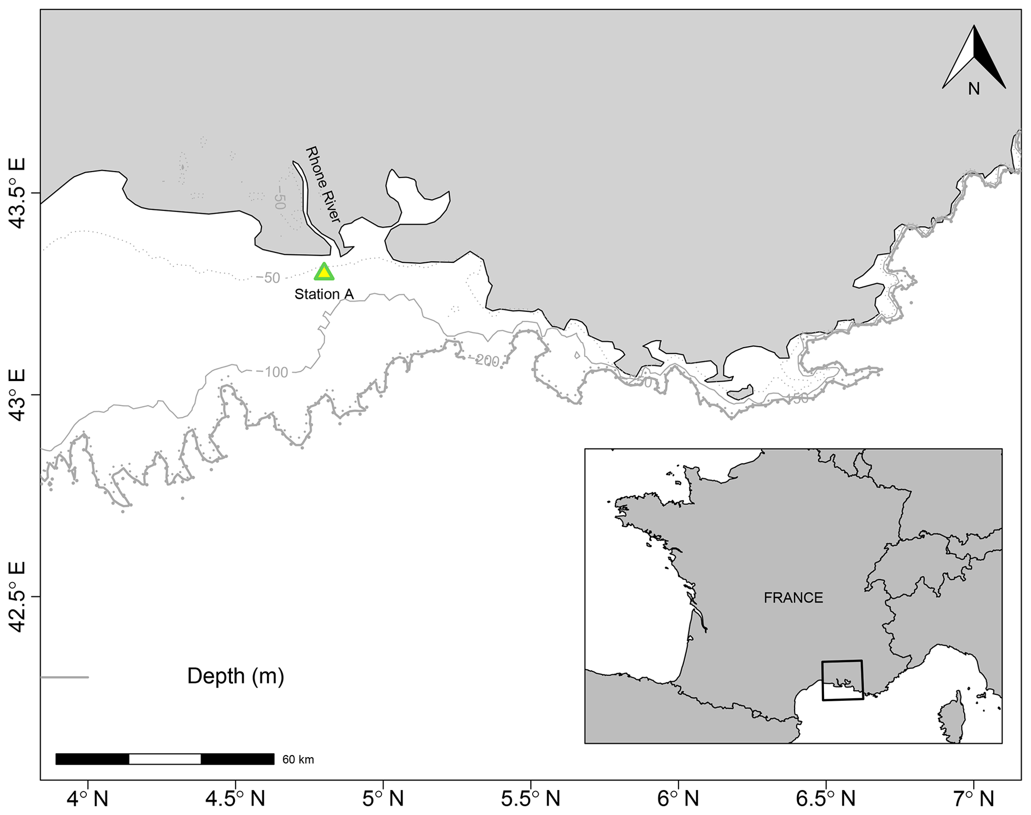
Figure 1Map showing the locations of sampling sites off the Rhône River mouth.
Relating to the episodic pulse of organic matter, numerous studies have documented instances of flood-driven deposition from the Rhône River from a hydrographic perspective (Boudet et al., 2017; Hensel et al., 1998; Pont et al., 2017). Pastor et al. (2018) go beyond sedimentology and hydrographic characteristics to provide a concise description of the various flood types, their diagenetic signatures, and biogeochemical implications. Furthermore, published porewater chemistry and solid-phase data have highlighted sediment characteristics following such an event (Cathalot et al., 2010; Toussaint et al., 2013; Cathalot et al., 2013; Pastor et al., 2018).
2.2 Model development and implementation
Following the description of the Rhône River flood types and the composition of the flood deposit (mainly in terms of organic carbon) at the proximal station A (Pastor et al., 2018), we proceed to describe the model developed to explore the observed data and their diagenetic implications in terms of relaxation times and their evolution following this transient perturbation.
Table 1Description of notations, phrases, acronyms, and abbreviations, as used in this paper.
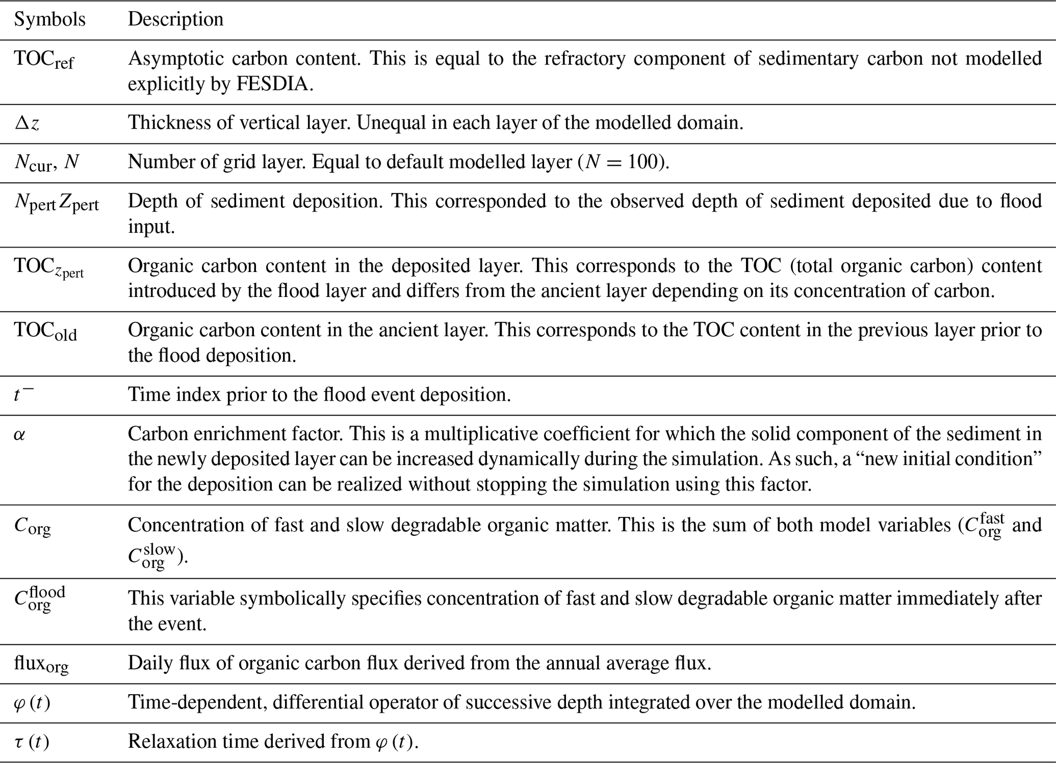
Our model combines the development in the OMEXDIA model (Soetaert et al., 1996a), applied in the Rhône prodelta area (Ait Ballagh et al., 2021; Pastor et al., 2011) and which has recently been equipped with event-driven processes (De Borger et al., 2021). In De Borger et al. (2021), the authors specifically addressed the issue of bottom trawling as a mixing and an erosional process that removes an upper layer of sediment and mixes a certain layer below. In addition, the model considers a bulk categorization of reduced substance in a single state variable, ODU (oxidative oxygen unit). For our approach, the event is defined by an addition of a new layer on top of the former sediment–water interface (Table 1). Furthermore, we explicitly modelled pathways involving sulfur and iron. Following this preamble, the following sections go over aspects of the model description and parameterization. Table 1 provide some key glossary of mathematical notations used in the model.
2.2.1 Model state variables
The complete model describes the concentration of labile () and semi-labile () decaying organic matter, oxygen (O2), nitrate (), ammonium (), and dissolved inorganic carbon (DIC), following the classic early diagenetic equation of Berner (1980) and Boudreau (1997). In addition to the model from De Borger et al. (2021), our model includes sulfate (), hydrogen sulfide (H2S), methane (CH4), and iron species (Fe2+ and Fe(OH)3) (Table 2).

In some coastal settings, oxidation via sulfate reduction has been highlighted as the primary pathway for organic carbon (OC) mineralization, with minor contributions from manganese and iron oxidation (Burdige and Komada, 2011). In addition, the flux of integrated remineralization products such as DIC has previously been estimated to contribute up to 8 times that of diffusive oxygen uptake (Rassmann et al., 2020) – thus highlighting its importance in describing the amplitude of benthic recycling in coastal water. As such in this paper, we focus our analysis on these proxy variables (O2, , DIC) because they serve as indicators of the integrated effect of the main diagenetic processes.
2.2.2 Biogeochemical reaction
Early diagenesis processes on the seafloor are driven by organic matter deposition. For areas such as the Rhône prodelta, continental organic carbon input is dominant, and it is difficult to identify the fraction of labile fraction responsible for fast OM pool consumption (Pastor et al., 2011). Moreover, observations show that some organic compounds are preferentially degraded and become selectively oxidized (Middelburg et al., 1997; Pozzato et al., 2018). As a result, the model assumed solid phase organic carbon with two reactive modelled fractions with different reactivities and ratios (Westrich and Berner, 1984; Soetaert et al., 1996a). The mineralization of OM occurs sequentially, with the labile fraction mineralizing faster than the slow decaying carbon. During the timescales considered here, the refractory organic matter class is not reactive. To compare with the observation, we consider an asymptotic OC constant (TOCref) for the inert fraction that scales the model-calculated TOC output to the observation (Pastor et al., 2011) (see Sect. 2.2.8). This organic carbon degradation requires oxidants, and the depth dependency in sequential utilization of terminal electron acceptors assumption first proposed by Froelich (1979) is used here. Oxygen is consumed first, followed by nitrate, iron oxides, sulfate, and finally methanogenesis occurs (Eq. 3). Because the quantity of organic matter and the relative proportions of fast and slow degrading materials decrease with depth, the overall organic matter degradation rate decreases accordingly. In the formulation of the individual biogeochemical processes, we use a similar paradigm as Soetaert et al. (1996a) (Eq. 2).
This rate of carbon mineralization of organic matter (mmol m−3 d−1) can be expressed as
where the rFast and rSlow are the decay rate constant (d−1) for fast and slow detritus component. ϕ and (1−ϕ) are the volume fraction for both solutes and solid respectively. This process is mediated by microorganisms and oxidant availability. The primary redox reaction includes (1) oxic respiration, (2) denitrification, (3) Fe (III) reduction, (4) sulfate reduction, and (5) methane production:
This reaction can be modelled using a Monod type relationship with each oxidant having a half-saturation constant (ks[C]) represented as ks* in the model code. The inhibition of mineralization by the presence of other oxidants is also modelled with a hyperbolic term (subtracted from 1), where kin[C] is concentration at which the rate drops to half of its maximal value. Using these limitation and inhibition functions, a single equation for each component across the model–depth domain can be realized (Rabouille and Gaillard, 1991; Soetaert et al., 1996a; Wang and Van Cappellen, 1996), together with some possible overlap (Froelich et al., 1979; Soetaert et al., 1996a). For a generic species, this can be described mathematically as
where C is one oxidant. Formulation for individual pathways as well as values of half-saturation and inhibition constants for each oxidant can be found in Appendix A1. With this limitation term, mineralization rate per solute can be estimated using potential carbon produced via OM degradation in (Eq. 1),
with the ∑lim the sum of all limitation terms which normalizes the term in order to always achieve the maximum degradation rate. See Soetaert et al. (1996a) for more details on the derivative of this equation.
Secondary redox reaction includes reoxidation of reduced substances (nitrification, Fe oxidation, H2S oxidation, methane oxidation) (Eq. 5) and the precipitation of FeS. Anaerobic oxidation of methane occurs in the absence of O2 following upward diffusion of methane to the sulfate–methane transition zone (SMTZ) (Jørgensen et al., 2019):
These reactions are mathematically described using a coupled reaction formulation. Nitrification is limited by the availability of oxygen and the other reactions are described with a first-order term.
where Rnit is the rate of nitrification (d−1), , , and are the maximum rate of oxidation of iron, sulfide, and methane via oxygen, respectively (mmol−1 m3 d−1). Because sulfide precipitation can occur in some coastal sediments, we accounted for this sink process by removing produced sulfide from sulfate reduction as a first-order FeS formation.
with RFeSprod the rate of production of FeS (mmol−1 m3 d−1).
2.2.3 Transport processes
Transport processes in the model are described by molecular diffusion and bio-irrigation for dissolved species whereas bioturbation is the main process for mixing the solid phase. In addition, advection occurs in both the solid and dissolved species. The model dynamics described as a partial differential equation (PDE) is the general reaction–transport equation (Berner, 1980). We use a similar paradigm and formulations to that of Soetaert et al. (1996a). For substances that are dissolved:
With special consideration of ammonium adsorption to sediment particles, the governing equation is given by
where we assumed that the immobilization of is in instantaneous, local equilibrium (i.e. any changes caused by the slow removal process results in an immediate adjustment of the equilibrium; so, can be modelled with a simple chemical species) and kads is the adsorption coefficient. The inclusion of this formulation for the diffusion and reaction term has the effect of slowing down ammonium migration in sediment. Derivation of this formulation is given in Berner (1980) and Soetaert and Herman (2009).
For the solid phase:
where C is the concentration of porewater (unit of mmol m−3 liquid) for Eq. (8) and S for solid (unit of mmol m−3 solid) Eq. (10). w (cm d−1) and Dsed (cm2 d−1) represent the burial/advection and molecular diffusion coefficient in the sediment respectively, and REAC is the source/sink processes linked to biogeochemical reactions in the sediment. This term includes both biological and chemical reaction within the sediment column and non-local bio-irrigation transport term (see next section). Db is the bioturbation term for solid driven by the activities of benthic organisms. For dynamic simulation, w can change as a function of time but in most cases we assumed a constant value.
Diffusive fluxes of solutes across the sediment–water interface are driven by the concentration gradients between the overlying seawater and the sediment column. Fick's first law is used to describe the solute flux due to molecular diffusion,
where the Dsed (cm d−1) is the effective diffusion coefficient corrected for tortuosity and given as , with Dsw the molecular diffusion coefficient of the solute in free solution of sea water, and θ is the tortuosity derived from the formation factor (F) and porosity (ϕ) of a sediment matrix (Berner, 1980; Boudreau, 1997). This molecular diffusion coefficient is calculated as function of temperature and salinity using compiled relation of Boudreau (1997), implemented in the R package Marelac (Soetaert and Petzoldt, 2020).
As a simplifying assumption, material accumulation has no effect on porosity. We further assumed the porosity profile decreased with depth but invariant with time. Although, this assumption is a restrictive as the site of flood deposition can undergo variation in grain size which might affect their porosity (Cathalot et al., 2010), we proceed noting that the fixed parameters which define the porosity curve can be changed when necessary. Thus, using optimized parameters fitted with data in the proximal sites of Rhône prodelta (Ait Ballagh et al., 2021), porosity (ϕ(z)) in Eqs. (10)–(8) is prescribed as an exponential decay,
where ϕ0 and ϕ∞ is the porosity surface and at deeper layer, respectively, while Zswi is the depth of the SWI (sediment–water interface), and δ (cm) is the porosity exponential decay coefficient with depth.
2.2.4 Bioturbation and bio-irrigation
Bioturbation in the model is characterized by the movement and mixing of particles by benthic organisms. This is parameterized as a diffusivity function in space (D(z)) and acts on the concentrations of the different solid species in the sediment. In our model, this bioturbation flux is assumed to be interphase, with porosity ϕ(z) remaining constant over time. Thus, this process is prescribed as
where is the bio-diffusivity coefficient (cm2 d−1) at the SWI and in the mixed layer, ZL is the depth of the mixed layer (cm), and biotatt is the attenuation coefficient (cm−1) of bioturbation below the mixed layer. D∞ is the diffusivity at the deeper layer as usually specified as zero. In the model, we did not account for mortality of benthic fauna following the deposition as in De Borger et al. (2021) where they focus on habitat recolonization after trawling.
Bio-irrigation is modelled in an identical manner to that of biodiffusion, and acts as a non-local exchange process between the porewater parcels and the overlying bottom water.
for which Irr0 is the bio-irrigation rate (d−1) and Irratt is the attenuation of irrigation (cm) below the depth of the irrigated layer Zirr (cm). At depth, the bio-irrigation rate (Irr∞) is generally set to zero.
2.2.5 Model vertical grid
The model is vertically resolved with grid divided into 100 layers (N), of thickness (Δz) increasing geometrically from 0.01 cm at the sediment–water interface to 6 cm at the lower boundary. The result is a 100 cm model domain comprising of a full grid with non-uniform spacing and maximum resolution near the SWI. Depth units are in centimetres. This choice of modelled depth allows for complete carbon degradation. This modelled grid is generated by the grid generation routine of the ReacTran R package (Soetaert and Meysman, 2012), which implements many grid types used in early diagenesis modelling. During the time instance of the event specification, the added grid of new layers (Npert≈Zpert) and the current grid (Ncur≈N) is rescaled to the model's common grid of N layer by linear interpolation (see Sect. 2.2.6 and Fig. S1). The concentration of state variables is defined at the layer midpoints, whereas diffusivities, advection (sinking/burial velocities), and resulting transport fluxes are defined at the layer interfaces.
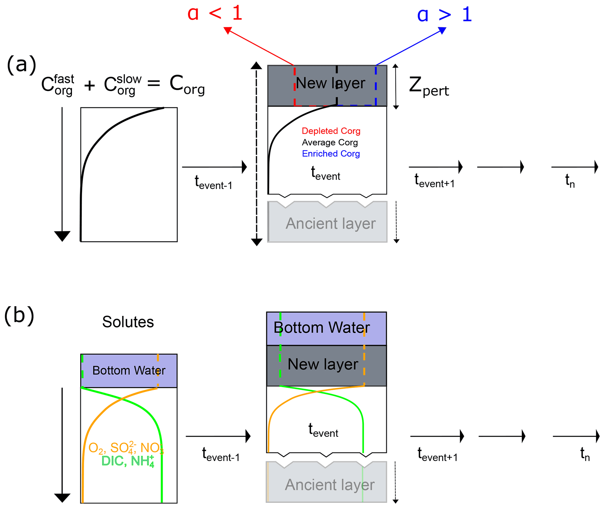
Figure 2Schematic of model implementation for the deposition event scenario. Profile from previous time step (left) and after addition of new layer over a predefined depth layer (right). For the solid (a), the new layer can be enriched (blue) or depleted (red) relative to the old (average) (black). The dissolved substances (b) are set equal to the bottom water concentration during the deposition. Thereafter, the profile is integrated forward with time. The whole sequence of step occurs dynamically with time capitalizing on the integrator ability to simulate dynamic event process. α is the carbon enrichment factor applied over depth Zpert (see text for detail).
2.2.6 Deposition event
The inclusion of the deposition event as a separate external routine to modify the sediment properties (i.e. porewater species, Corg) is a fundamental difference between our approach and the other previous early diagenesis model applied in the Rhone Delta, but it bears similarity with De Borger et al. (2021). We assume the event occurred as an instantaneous deposition of organic carbon ( and ) over a depositional layer, Zpert (Fig. 2).
The event calculation was carried out dynamically within the same simulation time. For the solid species, following the flux of organic carbon via the boundary condition (see Sect. 2.2.7), the portion of organic carbon is split between the fast and slow decaying component using a proportionality constant (pfast) as in Ait Ballagh et al. (2021). pfast varies from 0 to 1 and it is expressed in percentage of carbon flux deposited associated to either fraction (fast and slow). However, at the time when the event is prescribed, the integrated profile of the solid species and from previous time step, defined as (t−), was used to create a virtual composite of the deposited layer. This integral calculation was performed over a specified sediment thickness (Zpert), which corresponded to the vertical extent of the depositional event. This average concentration for the solid, which we define exclusively for the time of deposition as (), is scaled with an enrichment factor (α) (see below) and then nudged on top of the old layer which is supposed to be buried beneath after the event. To avoid numerical issues caused by the discontinuity of both layers with different properties, an interpolation of the composite profile was performed over the modelling domain. This smoothes the interface between the deposited layer's base and the current model grid's upper layer. This algorithmic procedure is schematically shown in Fig. 2 and we summarized this process mathematically as
where corresponds to the TOC content introduced by the flood layer and TOCold represents the TOC in the previous layer prior to the flood deposition. The carbon enrichment factor (α) in the model (confac in the model code) is introduced here in order to scale the deposited OC with those observed from field data. This helps in calibrating the deposited organic matter concentration ( and ) in the new layer relative to the previous sediment fraction, simulating the wide range of TOC content observed in the field. For instance, when the newly deposited organic matter is similar to the former sediment topmost layer (average pre-flood layer concentration over an equivalent Zpert depth), an (α) value of 1:1 is used. If the new material is lower in organic carbon content compared to what is near the sediment–water interface, then (α)<1, while if the newly deposited material is higher in carbon content than the sediment surface, (α)>1. This flexibility can be used to constrain the simulation to match the corresponding TOC profile from field observation. In the modelling application, this parameter is generally specified by using different value for the magnitude of OC in each fraction depending on the empirical observation of the TOC data. This quantity is therefore tunable and the upper bound of this parameter is dictated by the maximum TOC in the sediment sample.
It is important to note that this parameter differs from pfast. This OC flux partitioning by pfast occurs regardless of the event and it is related to the carbon flux received at the boundary, but the carbon enrichment factor occurs only during the event. The carbon enrichment factor (α) can be viewed as a method of imposing a new initial condition only at the time of the event by using the integral concentration from the previous time. However, using the approach described here, all calculations can be done dynamically without stopping the model.
For the solutes (O2, , , DIC, , H2S, and CH4), the bottom water concentration is imposed through the perturbed layer at the time of event by assuming this new layer is homogenously mixed.
2.2.7 Boundary Conditions
The boundary conditions for the model are of three types:
-
At the sediment–water interface, a Dirichlet concentration condition for most solutes equalling the bottom water concentration was used,
Both pore water and solid have a zero-flux boundary condition at the bottom of the model,
For solid, an imposed flux at the upper boundary for most of the year is used,
The model also includes the ability to include time-varying organic carbon flux with user-specific time series or a functional representation such as sinusoidal pattern. In the case study presented here, this carbon flux varies over the annual carbon flux () in the region in question. This was expressed mathematically as
At the time of the instantaneous deposition, this deposited carbon is treated as described in Sect. 2.2.6.
2.2.8 Model parameterization and verification
The model parameters in Table 2 (for full model parameter, see Table S1 in Supplement) were derived from previously published model in the Rhône Delta (Pastor et al., 2011; Ait Ballagh et al., 2021). The organic matter stoichiometry for both fractions is represented here by the NC ratio (NCrFdet and NCrSdet) with values of 0.14 and 0.1, respectively. The flux of carbon in the upper boundary of the model was defined using a yearly mean flux () of 150 mmol m−2 d−1 in Rhône prodelta (Pastor et al., 2011). TOC (in % dw) is estimated from both carbon fractions ( and ) assuming a sediment density (ρ) of 2.5 g cm−3 and conversion from the model unit for detrital carbon fraction of mmol m−3 to a unit in percent mass. The model diagnostics TOC value is then computed as follows:
with TOCref the asymptotic TOC value at deeper layer of the sediment, thus representing concentration of refractory carbon not explicitly modelled. The sedimentation rate used in this modelling study was kept constant at 0.027 cm d−1 (Pastor et al., 2011). The decay rate constant for the labile and semi-labile detritus matter is set as 0.1 and 0.0031 d−1, respectively, with both fractions split equally with a proportionality constant (pfast) of 0.5. Using parameters fitted by the model of Ait Ballagh et al. (2021) to data observed in the Rhône prodelta area, the rate of bioturbation and bio-irrigation is fixed as 0.01 cm2 d−1 and 0.23 d−1 with these fauna-induced activities occurring down to a depth of 5 and 7 cm, respectively.
The bottom water temperature was fixed at 20 ∘C. The bottom water salinity is nearly constant below the Rhône River plume, ranging from 37.8 to 38.2. In the model, the average temperature and salinity is used to calculate the diffusion coefficient for the solute chemical species (Sect. 2.2.3). Bottom water solute concentrations were constrained using previously reported values in previous modelling efforts (Ait Ballagh et al., 2021) and adapted with new data for the time corresponding to the flood deposit event (see Table 3). Porosity decreases exponentially with depth from 0.9 at the sediment water interface to 0.5 at deeper layer with a decay coefficient of 0.3 cm (Lansard et al., 2009).

For the verification of the model output, data from Pastor et al. (2018) corresponding to the diagenetic situation 26 d after an organic-rich flood were used. We restricted our benchmark to data from the proximal station (station A) near the river mouth, where the impact of this flood discharge is more visible (Fig. 1).
2.2.9 Numerical integration, application, and implementation
Because the procedure is based on OMEXDIA, complete details of the derivation can be found in that paper and is referenced therein (Soetaert et al., 1996a). Here we recap the mathematical formulation of the method of lines (MOLs) algorithm used by FESDIA. Direct differencing of Eqs. (8)–(10) results to
for a generic tracer C with a phase properties index Φ and DΦ denoting porosity and dispersive mixing term, respectively, for solid or liquid. This equation is calculated such that the variables and parameters are defined both at the centre of each layer zi and at the interface between layers . The position at the centre of the grid is then given as . Δzi represents the thickness of the i layer and is the distance between two consecutive grid layers. A Fiadeiro scheme (Fiadeiro and Veronis, 1977) based on the model's Peclet number (a dimensionless ratio expressing the relative importance of advective over dispersive processes) is used to set , thus providing a weighted difference of the transport terms which reduces numerical dispersion.
Equations (8)–(10) implemented as Eq. (22) are integrated in time using an implicit solver, called lsodes, that is part of the ODEPACK solvers (Hindmarsh, 1983). This solver uses a backward differentiation method (BDF); it has an adaptive time step, and is designed for solving systems of ordinary differential equations where the Jacobian matrix has an arbitrary sparse structure. The model output time and its time step (dt) is set by the user and is generally problem-specific. Because of the aforementioned challenge in observability of the massive flood event deposition, daily resolution is most often used for user dt. However, there is the possibility of obtaining higher resolution by decreasing dt.
The model application starts by estimating the steady-state condition of the
model using the high level command FESDIAperturb(). This steady-state condition is
calculated using iterative Newton–Raphson method (Press et al., 1992) and is
then used as a starting point for a dynamic simulation, with perturbation
times as in perturbTimes and depth of perturbation given as perturbDepth in the model function call.
As the event can be given as a deposit and mixing process, further
specification of the perturbation type (deposit or mix) is provided as an argument to
the simulation routine. In our case, we used only the deposit mode. The
event algorithm is used at the stated time point to estimate the model
porewater and solid properties driven by the instantaneous change in the
boundary condition. The concentrations are successively updated by their
diagenetic contributions during this time step. Afterward, this modified
profile is integrated forward in time. The model is written in Fortran for
speed and integrated using the R programming language (R Core Team, 2021)
via the “method of lines” approach (Boudreau, 1996). In addition, the
model made use of the event-handling capabilities' specific numerical solvers
written in the R deSolve package (Soetaert et al., 2010b). The R programming
language is used in the preprocessing routine for model grid generation
(Soetaert and Meysman, 2012), porewater chemistry parameter (Soetaert et
al., 2010a), steady-state calculation (Soetaert, 2014), and time integration
(Soetaert et al., 2010b). Further information about the model usage can be
found in the model-user vignette found in R-forge page (https://r-forge.r-project.org/R/?group_id=2422, last access: 2 August 2022).
2.2.10 Quantification of sediment diagenetic relaxation timescale
Quasi-relaxation timescale. Given the strong non-linearity and coupled nature of the biogeochemical system in question, we used an approximate approach to define the timescale of relaxation. Recognizing that in a nonlinear system, a perturbed trajectory is frequently arbitrarily divided into a fast, transient phase and a slow, asymptotic stage that closes in on the attractor (i.e. steady-state concentration; Kittel et al., 2017), we proceeded to estimate the relaxation timescale by using the time for which the memory of the perturbed signature disappears. We estimate the relaxation timescale by first calculating the absolute difference (φ(t)) between successive model output after the event, assuming that a slowly evolving state will eventually converge to the pre-perturbed state as time after the disturbance approaches infinity. This point-by-point concentration difference between two successive discretized profiles is then terminated at the point where the sum of absolute differences at each time point is less than the threshold (i.e. given by the median over the entire time duration). The relaxation time, τ, for each porewater profile species is then defined as the first time this threshold is crossed. A similar technique was employed by Rabouille and Gaillard (1990).
where N is the total number of grid point (i) used to discretize the depth profile (Xt), and Xt+1 is the depth profile at t+1 after the event.
This relaxation timescale calculation based on the disappearance of the perturbed signal (via successive profile similarity) may differ from an approach in which the profile returns to a pre-defined “old profile”. Because the exactness of pre-flood and post-flood profiles is difficult to quantify numerically (Wheatcroft, 1990), and the return to the former is frequently driven by slow dynamics, the approach used here can provide a window of estimate for which a particular signal fades toward the background of a theoretically pre-perturbed signal.
Uncertainty in relaxation timescale estimate. The uncertainty introduced by this technique is quantified using a non-parametric bootstrap of the τ statistics. The objective of bootstrapping is to estimate a parameter based on the data, such as a mean, median, or any scalar or vector statistics but with less restrictive assumptions about the form of the distribution that the observed data came from (Efron, 1992).
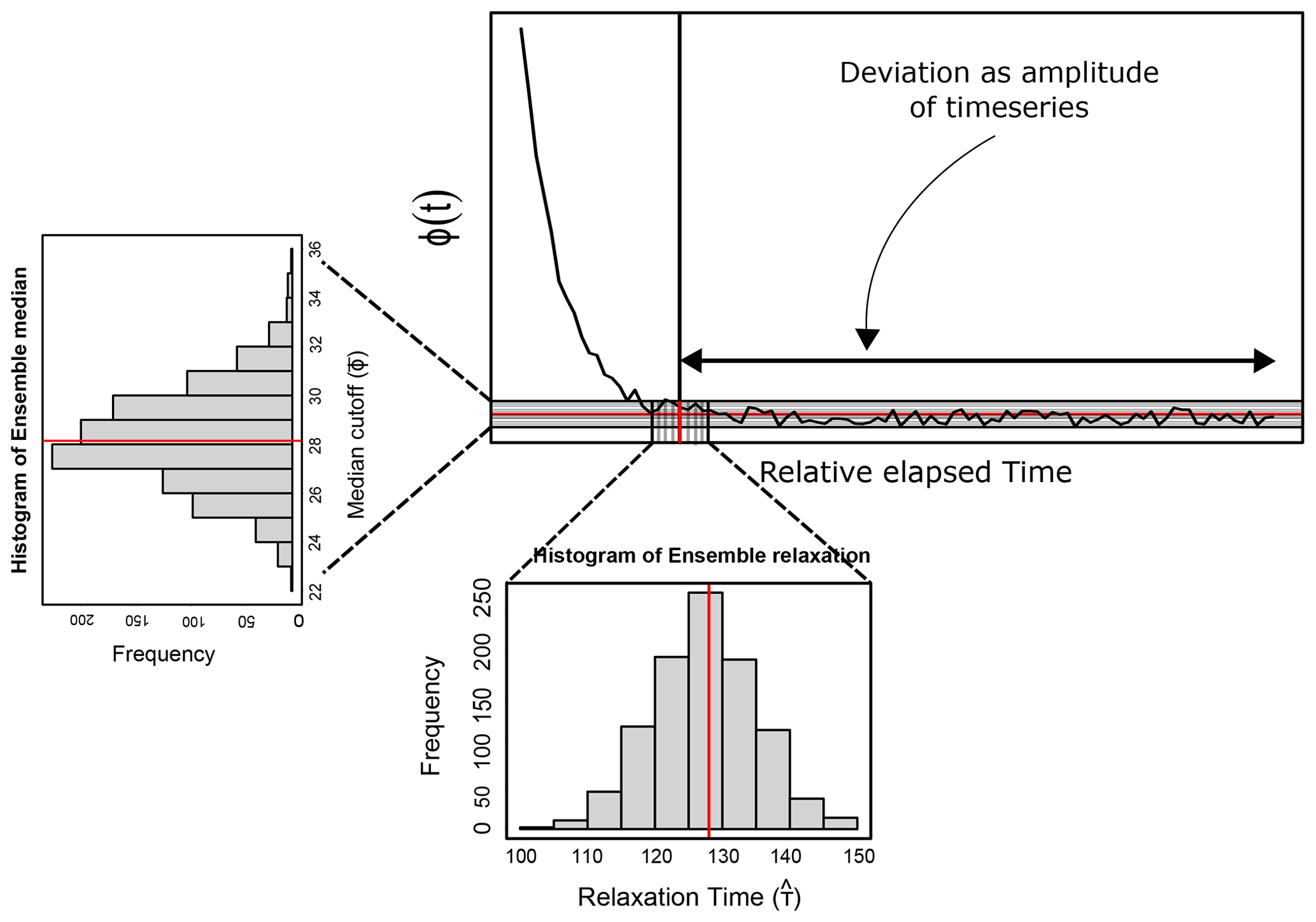
Figure 3The bootstrapping technique used to calculate the uncertainty in the relaxation timescale. The resampled median about a reference provides a replicate over which the standard error estimate is defined. The solid red represents the expected value of the quantity estimated while the vertical red line is the deviation from this expected value.
In this case, we employ a modified bootstrapping technique to estimate the uncertainty in the relaxation timescale by resampling on the cutoff point introduced in Eq. (23) (i.e. median, of a given reference simulation). This calculation takes advantage of the fact that the time series will be dominated by the slowly varying seasonal cycle over a long time period away from the point of perturbation, with the influence of the perturbation fading to the background. The variation of this reference time series over time reflects the uncertainty in this median threshold point. This variance, along with the reference cutoff value, can be used to generate n random perturbations varying about the normative threshold value. We can proceed to create a histogram of the replicate threshold(s) distribution. The histogram of this distribution is depicted schematically in the left margin of Fig. 3. The relaxation time in each realization of the threshold is calculated (). The median absolute deviation from this ensemble of relaxation times is then used to calculate the level of uncertainty in the statistics of interest (timescale of relaxation – ()). Figure 3 depicts this concept schematically. It should be noted that this method eliminates the need to rerun the deterministic model for each iteration, reducing the computational burden of this technique.
The 95 % confidence intervals ( and ) are reported in this paper by calculating the quantiles of this empirical distribution of .
2.2.11 Model simulation
The model is initialized as explained in Sect. 2.2.9. Thereafter, for the dynamic simulation, the model is spin-up for a sufficiently long time to attain dynamic equilibrium (≥5 years). A 2 yr run is carried out for the respective model application. The time step (dt) for dynamic simulation is daily in order to match the frequency for which observation of field data is possible. For specific numerical experiment, model configuration required for the simulation will be detailed in Sect. 2.2.11, “end-member type numerical experiment”.
End-member type numerical experiment
For the numerical model experiment, we investigate the sediment's response to two end-member types of deposition that can represent actual field observations in the Rhône prodelta (Pastor et al., 2018).
-
Low OC content with high sediment thickness scenario (EM1). In this scenario, we assume that a 30 cm new layer of sediment of degraded sediment was deposited. This scenario can describe old terrestrial material and is similar to the extreme case of flood event of May/June 2008 in the proximal outlet of Rhône River where lateral transfer of low TOC sediment (around 1 %) was deposited on top of the previously deposited sediment (OC around 1.5 %–3 %) (Cathalot et al., 2010). Using the partitioning of the carbon as explained in Sect. 2.2.7, an α value of 0.5 and 0.7 for and , respectively, was used to scale the TOC profile in order to mimic this type of trend.
-
High OC with low sediment thickness scenario (EM2). For this, we assumed a moderate 10 cm deposition of a new layer enriched in carbon during a flood discharge event. This scenario can correspond to the end-member case of November 2008 flood type with high TOC around 2.5 %, reaching more than 6 % in some sediment cores from the prodelta (Pastor et al., 2018), (most likely composed of freshwater phytoplankton detritus, debris, and freshly dead organisms) overlain on a less labile layer. In order to simulate this type of pattern, an α value of 20 and 10 for and , respectively, was used to adjust the TOC profile to such high-deposit OC scenario.
Except for the α and the thickness of the flood deposit, all other parameters were held constant in all numerical experiments. The time of the event occurrence in both scenarios were initialized at a period corresponding to published dates for May and November 2008 flood deposition as reported in Pastor et al. (2018). This helps to provide some realism to this hypothetical case study and appropriate context to the environmental regime when these events occur.
Sensitivity analysis
Lastly, we conducted a sensitivity analysis of the relaxation timescale for oxygen, sulfate, and DIC concentrations in terms of their variation to the thickness of the new sediment layer and the quantity of organic carbon introduced by the deposition.
We assumed a 15 cm average deposit thickness and conducted simulations with a thickness variation ranging from 1 to 30 cm. A 5 cm thickness increment was used for the sensitivity analysis. The α value is calculated in the same way: assuming a 1:1 ratio in the fast and slow OC fractions, and because deposited sediment can be highly refractory in nature, we geometrically conducted simulations with values ranging from 0.3 to 35. This was done only by changing the α corresponding to with the slow fraction fixed as 1. We also made sure that both series are equilateral in length, and that the values were chosen to span the range of values in EM1 and EM2, thus bracketing the normative value for the end-member case. This range encompasses the large spectrum of flood deposits such as those experienced in the Saguenay fjord, Canada (Deflandre et al., 2002; Mucci and Edenborn, 1992), the Rhône prodelta, France (Pastor et al., 2018), and in the Po River, Italy (Tesi et al., 2012).
3.1 Qualitative model performance: Cevenol flood in the Rhône prodelta
In order to compare the model evolution to field data, we made a comparison between the simulated profiles 26 d after a flood layer deposition and data collected in the Rhône prodelta in December 2008 (observed data collected 26 d after a Cevenol flood). During this flooding period, riverine discharge delivered 0.4×10⁶t of sediment which amounted to approximately 10 cm of sediment deposited in the site A of depocenter (Fig. 4).
The general pattern of the simulated profile agrees well with the observed data (Fig. 4). The newly introduced organic carbon-rich sediment resulted in rapid oxygen consumption. The data for total organic carbon (TOC) shown in Fig. 4 suggest a good agreement with the model, with high TOC (2.5 wt %–2.0 wt %) deposited at the upper 10 cm. Twenty-six days after the flood, the oxygen concentration dropped from 250 µM at the new sediment interface to nearly zero at 0.2 cm depth, and oxygen may have already returned to pre-flood levels; the simulated porewater profile was within the data's range (Fig. 4). The model diffusive flux of oxygen at this period was 18 mmol m−2 d−1 while the measured DOU (diffusive oxygen uptake) flux was 16.6±2.9 mmol m−2 d−1.
Overall, the model–data trend was satisfactory with observed depth distribution of sulfate () 26 d after the flood event fitted well, without much parameter fine-tuning. Only the sedimentation rate of the sediment was changed from 0.027 to 0.06 cm d−1 in order to match the observed distribution at depth. Sulfate reduction was high in the new layer. However, below the flood layer, the concentration in the data seem to asymptote to a value of 10 mM at 25 cm, while the model simulates complete sulfate depletion below 20 cm (Fig. 4).
The DIC profile shows a similar trend to the data collected after the flash flood. Within the depth interval of data, the model tends to follow the data. It drifts at lower depths, on the other hand, by overestimating the concentration of DIC observed at deeper layers. Similarly, the modelled shows a gradual increase with depth, and the model overestimates the production of below 15 cm (Fig. 4).
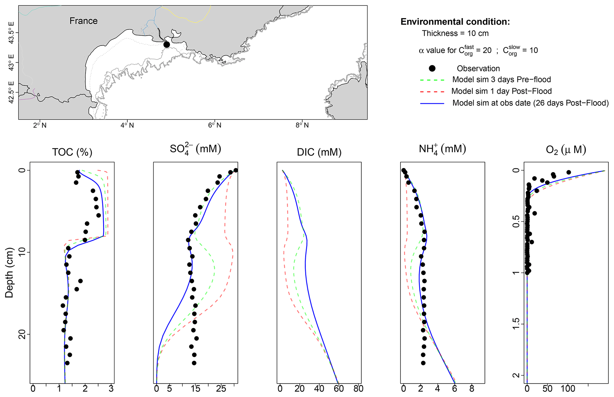
Figure 4Model and observation depth profile of TOC (%), SO, DIC,NH, and O2 for November/December event in station A (Rhône prodelta). The green and red dashed lines depict the vertical depth profile of the model before (3 d) and after (1 d) the flood deposit. The blue solid line represents the model result on the day the observations were collected (26 d after the flood, as indicated by the black circle).
3.2 Numerical experiment on end-member scenarios
3.2.1 Low carbon, high thickness scenario (EM1)
With a test case of 30 cm of new material deposited during the event (EM1) in the spring, the sediment changes as thus: prior to the event, the oxygen penetration depth (OPD) was about 0.17 cm. The OPD increases to 1.17 cm after the deposition of these low OC materials. The model showed a gradual return to its previous profile within days, with the OPD shoaling linearly with time (Table 4). By day 5, oxygen has returned to the pre-flood profile with similar gradient to the pre-flood state.
Against a background OM flux following the introduction of the flood layer, the sediment responded quickly. As a result, the perturbation has a significant effect on sulfate penetration depth, with concentration remaining nearly constant within the perturbed depth (≈20 cm). This corresponds to the bottom water concentration (30 mM) trapped within the flood deposit. Within that layer, sulfate reduction rate was low with an estimated integrated rate of 2.14 mmol C m−2 d−1 from the surface to 30 cm.
Table 4Model vs. data comparison for oxygen penetration depth (OPD), flux of oxygen, sulfate, and DIC (26 d after deposition).
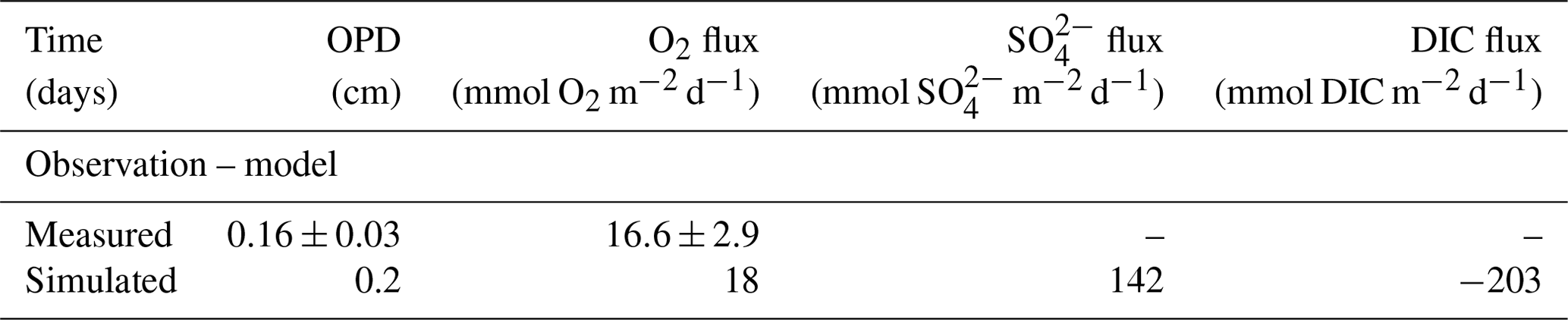
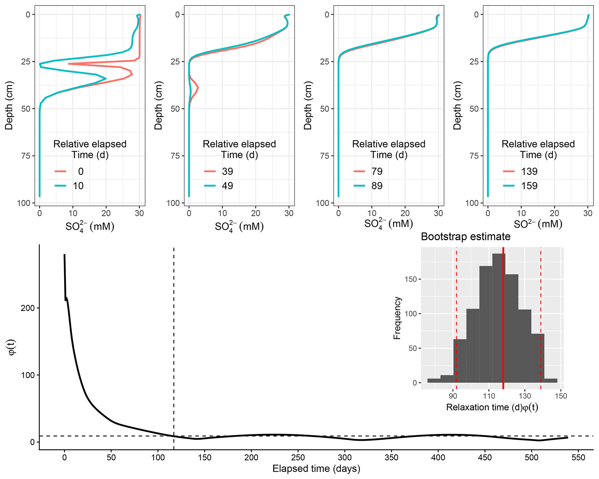
Figure 5Scenario 1 (EM1): model evolution for sulfate following deposition. Relative deviation of successive profile with time shown below. Dashed vertical line signifies cutoff point by the median (dashed horizontal line). Inset: histogram of bootstrap estimate of sulfate relaxation timescale for EM1 with 95 % confidence interval.
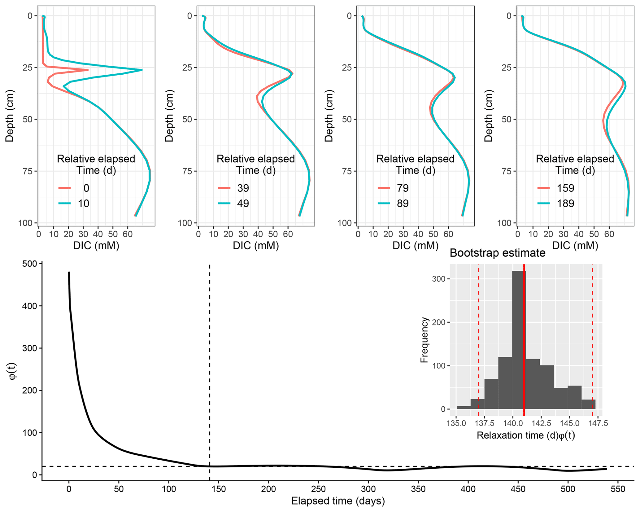
Figure 6Scenario 1 (EM1): model evolution for DIC following deposition. Relative deviation of successive profile with time shown below. Dashed vertical line signifies cutoff point by the median (dashed horizontal line). Inset: histogram of bootstrap estimate of DIC relaxation timescale for EM1 with 95 % confidence interval.
Below the interface with the newly deposited layer, the sediment is enriched in OM whose mineralization results in a higher sulfate reduction rate (SRR) at the boundary that delineates the newly deposited layer and the former sediment–water interface. The simulated SRR falls from 437 mmol C m−3 d−1 at the former sediment–water interface (now re-located at 26 cm) to 24 mmol C m−3 solid d−1. This high interior sulfate consumption at the boundary correlates well with the higher proportion of reactive organic material buried by the new layer containing less reactive material. From day 10, the consumption of this OM stock by sulfate controls the shape of the profile (Fig. 5). This anoxic mineralization via sulfate reduction will continue until the entire stock of carbon is depleted 50 d after deposition. Following that, OM mineralization via sulfate reduction shift becomes more intense at the top layer by day 60 (2 months after the event), when it begins to gradually evolve to the typical depth-decreasing sulfate profile. By day 115 (∼4 months), the profile had almost completely returned to its pre-flood state. We estimate that it took approximately 4 months for sulfate to relax back to within the range of background variability (with lower and upper bootstrap estimate between 92–139 d).
Correspondingly, OC mineralization products (such as DIC) were significantly lower in the upper newly deposited layer, as a consequence of the reduced quantity of OC brought by the flood. This concentration increased with depth to about 80 mM. Starting from the deposition, higher production of DIC below the former SWI led to a distinct boundary in the sediment: a DIC-depleted layer above an increasing DIC with concentrations up to 75 mM trapped in the region below the new–old sediment horizon 20 d after deposition (Fig. 6). This increased DIC production continued despite complete exhaustion of buried labile fraction with mineralization driven by the slow decaying component. The depth gradient caused by the increased DIC production enhances diffusive DIC flux. Following that initial period, DIC began to revert to its previous state. This slow re-organization, mostly driven by diffusion continues, with an estimated recovery time of 5 months (with a 95 % bootstrap confidence interval of 137–147 d respectively), as it temporarily lags behind in its return to the previous pre-flood state.
3.2.2 High carbon, low thickness scenario (EM2)
A flood deposition scenario of 10 cm thick material with enhanced OC content was used for the other end-member case experiment (EM2) in autumn. In this scenario, the modelled sediment exhibits a variety of response characteristics. The newly introduced sediment resulted in rapid oxygen consumption. The OPD decreased to 0.74 cm shortly after the event, according to the model, and stabilized there for days. There was no visible deformation in the shape of oxygen during its recovery trajectory, and total oxygen consumption for organic matter mineralization decreased by 8 % during the first 2 d after the event, from 12 to 11 mmol O2 m−2 d−1.
The concentration that developed as a result of the deposition showed two gradients: a concentration gradient from 30 mM at the “new” sediment water interface to 26 mM in the newly deposited layer (Fig. 7). Accordingly, the DIC in the corresponding depth layer gradually increased up to 20 mM (Fig. 8). An intermittent increase in was simulated below the new interface, at the boundary with the “old” sediment–water interface (SWI), reaching up to 29 mM from 9 to 12 cm (Fig. 7). This layer, which corresponded to the depth horizon where the new layer gradually mixed with the old layer, resulted in less sulfate reduction and DIC production in comparison to the new layer. Porewater concentrations decreased monotonically with depth from this interface, with a corresponding increase in DIC. Within 26 d of the event, the sulfate profile appears to be returning to its original shape. By then, 75 % of the newly introduced fraction of OM had been depleted, with OM remineralization in the upper layer fuelled by the small amount of remaining detrital materials. As the temporal memory of the deposition fades, the profile continues to gradually evolve towards the background, fed by the slow decaying OM, up to day 90, when the sulfate profile appears to have reached a similar pre-flood state. In this scenario, the estimated and DIC relaxation timescales were around 3 months (91 d for and 102 d for DIC) (Fig. 7).
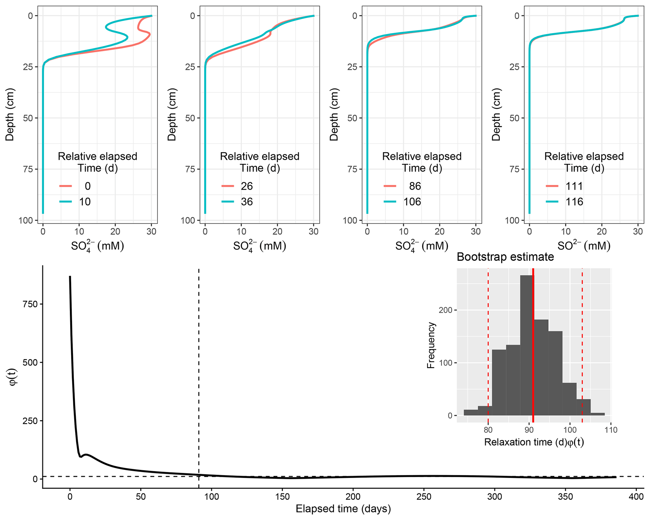
Figure 7Scenario 2 (EM2): model evolution for sulfate following deposition. Relative deviation of successive profile with time shown below. Dashed vertical line signifies cutoff point by the median (dashed horizontal line). Inset: histogram of bootstrap estimate of sulfate relaxation timescale for EM2 with 95 % confidence interval.
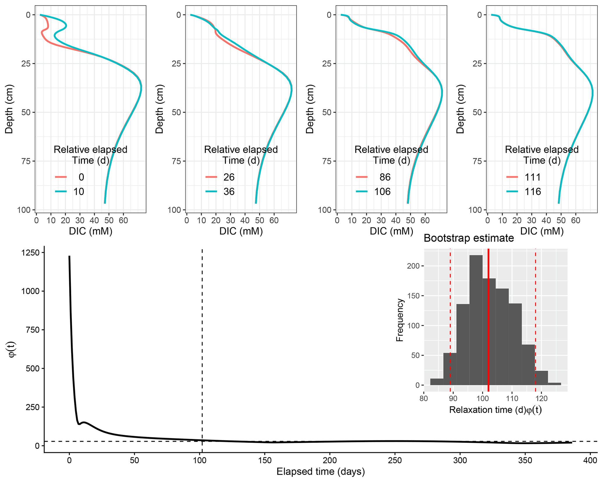
Figure 8Scenario 2 (EM2): model evolution for DIC following deposition. Relative deviation of successive profile with time shown below. Dashed vertical line signify cutoff point by the median (dashed horizontal line). Inset: histogram of bootstrap estimate of DIC relaxation timescale for EM2 with 95 % confidence interval.
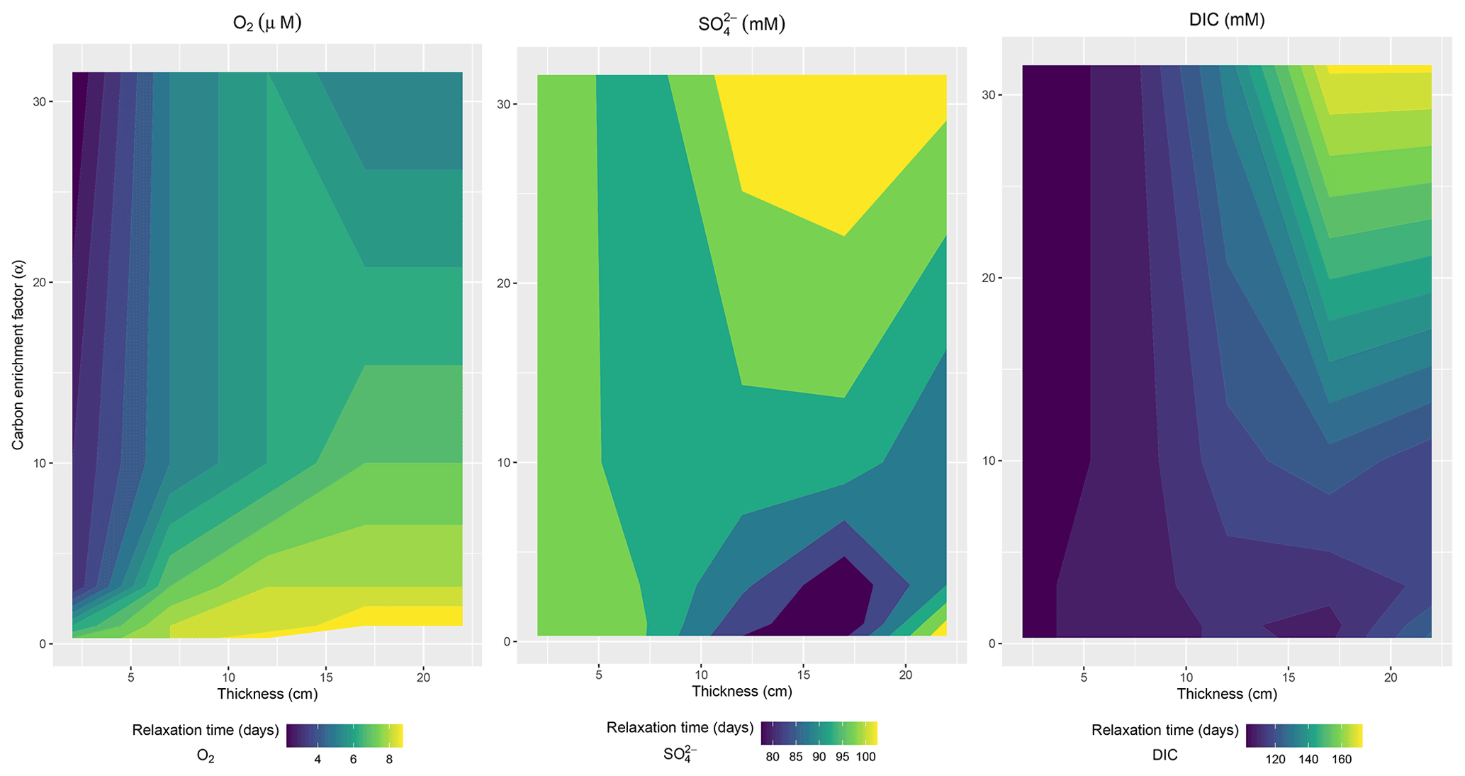
Figure 9Relaxation timescale (τ) in days as function of deposited sediment thickness and enrichment factor (α) for degradable OM.
3.3 Sensitivity of relaxation time to variation in enrichment factor (α) and sediment thickness (zpert)
We then examine the sensitivity analysis of the relaxation timescale (τ) for oxygen, sulfate, and DIC for variation in sediment deposit thickness (Zpert) and the concentration factor for enrichment (α) covering values ranging between the two EM scenarios.
Over all runs varying the enrichment factor (α) and the thickness of the flood input layer, relaxation time for oxygen varied from 2 d for a flood-deposited layer consisting of a thin layer of high concentration of labile OC to 9 d for a thicker deposited layer with low concentration of labile OC. In contrast, the relaxation timescales for and DIC were significantly longer than those for O2 (3 to 4 months). In addition, the relaxation timescale surface structure for appears complex with divergence gradient at mid-depth of 15 cm. For deposited depth layers above 5 cm and at low α value, the relaxation time for varied between 75–100 d (2–3 months). Below 5 cm (bioturbated depth imposed in the model), relaxation time was constant across all α variations (100 d). As organic enrichment (α) and thickness increase, the model estimates a longer relaxation time with a maximum time span of 105 d.
Similar variation of relaxation time for DIC was simulated for different α and sediment deposit thickness. However, unlike , relaxation time for DIC varies smoothly across the range of α and thickness combinations with relatively constant relaxation time (100 d) at low thickness and α combinations. The relaxation time increased exponentially as sediment deposit thickness and labile OC concentration increased (α), with maximum recovery time (171 d/6 months) simulated at the extremes of both combinations (Fig. 9).
In highly dynamic coastal ecosystems, such as RiOmar (river-dominated ocean margins) systems, driven by seasonal variability and meteorologically extreme events, the response of early diagenetic processes to time varying deposition of organic matter is generally non-stationary (Tesi et al., 2012). While dynamic equilibrium as a steady-state condition may be reasonable in the case of seasonal variability, such an assumption may fail in cases of instantaneously event-driven deposition. An intermittent supply of sediment and OC, like those presented here, can cause a change in the system's properties on a short- or long-term basis. Previous works have highlighted excursions in sediment redox boundary (Katsev et al., 2006), flux of solutes at the sediment–water interface (Rabouille and Gaillard, 1990), and modification of other system properties due to depositional flux of organic matter. Thus, the premise of steady-state conditions in early diagenetic processes which often depends on the temporal resolution of the observation might need revisiting especially in areas of episodic sedimentation (Wheatcroft, 1990; Tesi et al., 2012). Here, we discuss the evolution and dynamics of a non-stationary sedimentary system following a singular perturbation.
4.1 Model representation and utility
Non-steady-state models are increasingly being applied in dynamic coastal environments, but they are still primarily based on forcing from smooth varying boundaries that mimic seasonal forcing or long-term variability (Soetaert et al., 1996b; Rabouille et al., 2001a; Zindorf et al., 2021). Explicit consideration of abrupt changes in the upper boundary of the model caused by events such as landslides, flash flooding, turbiditic transfer of materials on a continental slope, and trawling is still relatively uncaptured by these models (but see De Borger et al., 2021, for inclusion of erosion events). In this paper, we adapt OMEXDIA (Soetaert et al., 1996a), a well-known reaction transport model, to investigate the changes in the solid and liquid phases during massive deposition event. Our efforts highlight the algorithm's utility in incorporating this process with minimal numerical issues. The model represented the basic characteristics of the data derived from the November/December 2008 flood event at station A in the Rhône Delta's depocenter (Fig. 4). The simulated flux was also in agreement with the estimate from field data, as diffusive oxygen uptake (DOU) rate sampled 26 d after the event (8 December 2008) was 16.6±2.9 mmol m−2 d−1 (Cathalot et al., 2010) while the estimate from the model was 18 mmol m−2 d−1. As the inclusion of such discontinuity in PDE(s) presents numerical challenges in classic solvers, the implementation utilized by our model ensures such difficulties are overcome. This is the result of improved development of solvers adapted to such a problem (Soetaert et al., 2010b). This difference in the approach employed here distinguishes ours from other published models (e.g. Berg et al., 2003; van de Velde et al., 2018) with similar scientific motivation for time-dependent simulation. Overall, the validation of the model output with field observations lends some confidence in using the model in scenarios involving abrupt changes in boundary conditions and investigating biogeochemical changes in the sediment as a result of such an event. This is despite the model underestimation of the amplitude of sulfate and DIC at depth which can be improved with better optimization of some parameters, especially those derived from previous studies that might not be suited for such a flooding regime or with better process resolution relating to these pathways. Nonetheless, there are advantages to this model especially in the case of episodic flood deposit events, where only a snapshot of data is available at any given time. Modelling tools capable of simulating this event with high fidelity can provide continuous information of the system state and help fill in data gaps needed to understand the sediment's response on different timescales.
4.2 Role of end-member flood input OM in the diagenetic relaxation dynamics
Flooding events can transport large amounts of material through the river to transitional coastal environments such as deltas and estuaries. River floods can account for up to 80 % of terrigenous particle inputs (Antonelli et al., 2008; Zebracki et al., 2015), and they can have a significant impact on geomorphology (Meybeck et al., 2007), ecosystem response, and biogeochemical cycles (Mermex Group et al., 2011). If the source materials have a different organic matter composition (Dezzeo et al., 2000; Cathalot et al., 2013), the rapid deposition of these flood materials can alter diagenetic reactions and resulting fluxes.
Furthermore, the relaxation timescale associated with the sediment recovery following this external perturbation can be important in terms of the process affecting the biogeochemistry of solid and solutes species. With a series of numerical experiments ranging in between two end-members of the input spectrum for flood events such as those in the Rhône prodelta (Pastor et al., 2018), our study revealed contrasting sedimentary responses and associated typical timescales at which porewater profiles relax back to undisturbed state. Using a simple metric for estimating relaxation timescale of the perturbation, our calculations for the first end-member scenario (EM1) show that the upper bound of the timescale of relaxation for oxygen is 5±3 d, whereas it was approximately 2±2 d for the second end-member scenario (EM2). This reflects the property of oxygen, which quickly approaches a steady-state situation after an event (Aller, 1998). This viewpoint is supported by an ex situ controlled laboratory setup. In their studies, Chaillou et al. (2007) demonstrated that after gravity-levelled sediment was introduced, oxygen consumption quickly recovered to its first-day level, with a sharp response time of 50 min and gradual shoaling of OPD within 5 d. We conclude that the tiny difference in oxygen relaxation and diagenetic response between the two scenarios can be attributed to the slow kinetic degradability of the refractory carbon deposited in the first scenario versus the labile nature of the deposit in the second scenario. This kinetically driven OM degradation has been extensively studied and provides the basis for the reactive continuum in early diagenesis models (Middelburg, 1989; Jørgensen and Revsbech, 1985; Burdige, 1991).
Other terminal electron acceptors (TEAs), such as , relax toward natural variation over a longer timescale than oxygen. For EM1, our simulation predicts a sulfate relaxation time of 117 d with a 95 % confidence interval (CI) estimate between 92 d (lower CI) and 139 d (upper CI) while in the case of EM2, we estimate a sulfate relaxation time of 91 d with comparatively low temporal variability (lower CI–80 and upper CI–103 d). This difference in relaxation time is caused by the differences in sediment characteristics and how their mineralization occurs over the sediment layer. In the first scenario, organic-rich sediment is buried by less reactive new material. The buried sulfate fraction is reduced faster than in the new layer above and controls the short-term recovery. As the buried carbon stock depletes and the physical imprint of the flood deposition fades, the profile begins to revert to its pre-flood shape. The post-flood evolution for the second scenario (EM2), on the other hand, differs in that the OM is consumed in the classical manner, with decreasing sulfate consumption with depth, caused by top-down control of the OM flux that adds OM to the sediment surface.
Such a long time lapse for the recovery of an element with a complex pathway, such as , has been reported in the literature (Anschutz et al., 2002; Stumm and Morgan, 2012; Chaillou et al., 2007). Similarly, estimates from our simulation for each end-member scenario indicate that mineralization products such as DIC have a longer relaxation time. This is especially true for the first scenario as opposed to the second, with evidence of slow convergence at depth within the simulation timescale for the first scenario. We estimate that DIC will recover to its pre-deposition state in 5 months for EM1 and in a comparatively shorter time for EM2 (3 months). This lag in DIC recovery could be attributed to the fact that its post-flood dynamics is governed by the slow decaying detrital material that contribute to the already buried refractory carbon. This long-term quasi-static behaviour of the porewater concentration despite such dynamic introduction of flood input can be understood by introducing the concept of a biogeochemical attractor effect – a similar analogy to the Lorenz attractor (Lorenz, 1963). This idea is derived from the mathematical theory that describes chaos in the real world (Strogatz, 2018; Ghil, 2019). The existence of a “biogeochemical attractor” may explain why multiple temporal data sets in the Rhône River prodelta show a similar diagenetic signature from spring to summer (Rassmann et al., 2016; Dumoulin et al., 2018). Our timescale analysis estimates that such rapid system restoration is indeed plausible and of the correct order of magnitude, based on the range of uncertainty reported here.
In addition, our calculations show that the timescale of return to the previous “pre-flood” profile is bracketed by the range of recovery due to purely molecular diffusion, putting an upper bound on our estimate. For example, using the Einstein's approximation, a species such as oxygen with a sediment diffusion coefficient (Ds) of 1.52 cm2 d−1 takes approximately 300 d to be transported solely by diffusion through a 30 cm sediment column and approximately 30 d for a 10 cm sediment column. Similar scaling argument could be made for species such as (Ds=0.86 cm2 d−1) with >500 d to be transported through 30 cm and ≈60 d for 10 cm. Because our estimates are less than these values, it suggests that processes other than diffusion (thickness effect) may contribute to relaxation control. It emphasizes the importance of biogeochemistry (OM kinetic) in modulating the response after the event. Besides that, any long-term recovery timescale is governed by the solid deposited. In comparison to the timescale of relaxation roughly estimated from field data (Cathalot et al., 2010), our estimate shows the right order of magnitude.
The relaxation time may also vary depending on the diagenetic interaction, and the characteristics of the organic matter available for degradation. This difference in characteristics was partially imposed in our study by assuming variations of α in the new deposit. The empirical observation of sediment characteristics associated with flood input dictates this parametric turning to match the TOC characteristics (Pastor et al., 2018; Deflandre et al., 2002; Mucci and Edenborn, 1992; Tesi et al., 2012; Bourgeois et al., 2011). However, more data from the field and laboratory experiments that resolve the OM composition of flood deposits are required to constrain the choice of this numerical parameter.
4.3 Control of relaxation time by sediment deposit properties
With the sensitivity analysis, we further explore the variation of relaxation timescale under variation of the thickness of layer and enrichment factor of input material given by α in our model. The model's sensitivity analysis reveals that the thickness and concentration of the reactive fraction of TOC control the relaxation time across a wide range of deposited sediment perturbation characteristics (Fig. 9).
In terms of the recovery time as a function of the availability of labile OC, our results revealed a contrasting pattern for oxygen and sulfate. Several factors related to how different oxidants react with sediment matrix disturbances can explain these differences:
-
With oxygen that has a high molecular diffusion coefficient, variations in relaxation time depend on the levels of labile OC, with thin sediments containing a high level of labile OC showing a shorter recovery time than thicker sediments with a low OC content. This pattern can be attributed to the higher relative importance of oxygen consumption in OM-poor sediment relative to the OM-rich sediment.
-
For low thickness deposits, sulfate and DIC relaxation times were more or less constant. However, a longer relaxation time was simulated for larger deposits and higher labile OC. This can be attributed to the increased distance required for solutes to migrate back after the event. This is clearly the case for sediment thicknesses greater than 14 cm. Such two-way dynamics could be explained by the fact that biological reworking and physical mixing within the surface mixing layer (SML) can improve OC degradation by promoting the replenishment of electron acceptors (i.e. oxygen, sulfate, nitrate, and metal oxyhydroxides) (Aller and Aller, 1992; Aller, 2004), resulting in a shorter recovery time for the porewater profile to reorganize within the SML.
This critical depth could also be the distance horizon at which the slow diffusion of the profile when retracting back to its pre-flood profile becomes an important factor in controlling the relaxation timescale. This is especially true for DIC, where the connection is more obvious. It has been proposed that when flood deposits extend beyond the sediment bio-mixing depth, the relaxation time for the constituent species is determined by the concentration gradient between the historical and newly deposited layers (Wheatcroft, 1990). In our sensitivity analysis, higher α corresponds to higher concentrations at depth, resulting in a case of enhanced OC degradation (both at the surface and within the sediment matrix). This depletes electron acceptors such as sulfate, which are required for OM mineralization at this depth. The slow diffusion across the displaced distance, on the other hand, cannot quickly compensate for its demands, which may explain the longer relaxation time. In other words, a higher concentration of OC in a region where all oxidants are nearly consumed results in a profile that takes a relatively longer time to recover to its previous state due to the constraints imposed by oxidant availability. This viewpoint is consistent with previous research from the Rhône prodelta area, where a minimum transport distance of 20 cm is suggested for efficient connection with the SWI; above which several processes are decoupled (Rassmann et al., 2020) and other eutrophic systems, where evidence of large accumulation of organic matter in subsurface sediments serves as a constraint on system restoration (Mayer, 1994; Pusceddu et al., 2009). Indeed, more observational and experimental studies are needed to better understand these processes.
4.4 Model limitations and future development
Because it is based on the well-established OMEXDIA model, FESDIA has several capabilities that make it suitable for a wide range of application domains for non-steady-state early diagenetic simulation. However, due to assumptions made during model development, some limitations in model usage must be considered:
-
First, we assumed that porosity is time independent. This may not be the case in some coastal systems that receive sediment materials from regions with distributary channels, which contribute particles of varying origin and grain size (Grenz et al., 2003; Cathalot et al., 2010). The composite sediment that is eventually transported to the depocenter by a flood event may differ in porosity, and thus vary temporarily depending on when and where the source materials are derived during the flood event. In this case, model estimates of fluxes in dissolved species may be over/underestimated. The resulting porosity in the new layer is barely predictable and could range between 0.65 and 0.85 in the proximal zone of the prodelta (Grenz et al., 2003; Cathalot et al., 2010), allowing us to justify our assumption.
-
Second, in our examples, we assumed that the burial rate and bioturbation were constant. With the introduction of these flood events, such assumptions may be called into question (Tesi et al., 2012). In addition, benthic animals respond to other perturbation event such as trawling in ways that may warrant explicit description of their recovery, which is linked to bioturbation (De Borger et al., 2021; Sciberras et al., 2018). While some coastal sediment burial rates have been shown to vary seasonally (Soetaert et al., 1996b; Boudreau, 1994), in the proximal zone of the Rhône prodelta, approximately 75 % of sediment deposition can occur during the flood (e.g. 30 cm d−1), with the remaining 25 % distributed throughout the year at a low range daily constant rate (0.03 cm d−1). The dominance of flood deposition over non-flood sedimentation, and the low bioturbation rate observed in the Rhône prodelta (Pastor et al., 2011), prompted the use of constant rate in the application shown here. Moreover, we designed the FESDIA model to allow for the use of a temporarily varying rate constant and coefficient for these processes, and the possibility of imposing an observational time series in cases where such data exist.
The current FESDIA version does not include a diffusive boundary layer, which can be important for material exchange between the overlying bottom water and the sediment. This is critical for calculating fluxes of species such as O2, where the depth extent of the DBL (diffusive boundary layer) zone is comparable to the depth at which oxygen consumption occurs (Boudreau and Jorgensen, 2001). As a result, the current version of FESDIA may overestimate the flux of O2. However, because the primary focus of this paper is on the relaxation dynamics of species (SO and DIC), where the DBL has negligible impact on the relaxation time and overall diagenetic processes (Boudreau and Jorgensen, 2001), the simplification presented here is justified. Even for oxygen, the inclusion of DBL which might result to corresponding change in the concentration at the SWI only have a marginal effect on its relaxation time (<2 d – within the range of uncertainty reported here), so the conclusions drawn in the case studies discussed here are still valid.
In terms of future development, we hope to improve the model's diagenetic pathways, particularly for the iron and sulfur cycles. Furthermore, processes such as calcite formation have been shown to affect DIC profile by 10 %–15 % in the proximal sites of Rhône prodelta (Rassmann et al., 2020), thus might necessitate inclusion in future versions of the model. This will enable FESDIA to account for carbonate system dynamics in marine sediment which can play an important role in the coast carbon cycle (Krumins et al., 2013).
4.5 Relaxation time metric: limitation and perspective
While one main focus of this study is on providing a quantitative estimate of relaxation time, the difficulty of objectively defining what relaxation means necessitates some commentary. This difficulty is not unique to marine biogeochemistry, as accurate quantification of recovery time is an open research question in other fields. In the context of a sedimentary system, Wheatcroft (1990) proposed that determining “dissipation time” (analogous to our “relaxation time”) can be subjective when it comes to signal preservation after sediment event layer deposition. The difficulties are exacerbated by previous work on episodic pulse on sediment biogeochemistry (Rabouille and Gaillard, 1990), in which two metrics for estimating relaxation timescale for silica were proposed. Outside of benthic early diagenesis, Kittel et al. (2017) proposed two generic metrics for systems with well-defined asymptotic properties that can be applied to a distance function from a given target (subject to certain mathematical assumptions). Because porewater profiles are inherently nonlinear, and biogeochemical pathways in sediment are tightly coupled, the mathematical suggestion of asymptoticity using such a distance metric for an evolving profile converging toward the target proposed in that paper is frequently not met. This is the case for our investigation. Overall, while we provide a first-order approximation of relaxation time following perturbation for some model-state variables, these studies highlight also some of the challenges associated with defining the timescale at which a signal can be validly assumed to have returned to its prior state. However, our method allows a full discussion of relaxation times for the main biogeochemical pathways.
The need to comprehend extreme events and their relationship to marine biogeochemistry prompted the development of novel methods for diagnosing flood-driven organic matter pulses in coastal environments. In this paper, we propose a new model (FESDIA) for characterizing flood deposition events and the biogeochemical changes that result from them. This type of event can have an impact on the benthic communities and the response of the whole ecosystem (Smith et al., 2018; Bissett et al., 2007; Gooday, 2002). Our modelling study shows that the post-depositional sediment response varies depending on the input characteristics of the layer deposit. For instance, we tested the combined effect of enrichment of labile organic carbon and deposit thickness on space–time distribution and relaxation time of key dissolved species (oxygen, sulfate, DIC). This integral timescale of relaxation is constrained by the intrinsic properties of the solutes (diffusion) and the characteristics of the flood input (thickness and concentration of labile organic carbon). In essence, the findings from this study highlight the importance of the quantity and quality of organic carbon in modulating the sediment response following such a singular perturbation, and the role of flood events with heterogeneous quantitative contributions in the coastal ocean.
A1 Biogeochemical reaction
The full model equation explained in Sect. 2.3.2 is described fully below. Organic matter is composed of three fractions: fast degradable organic matter, slow degradable organic matter, and refractory organic matter. Given the long timescale for the degradability of the refractory OM, it is parameterized using TOCref as the asymptotic value. For the two other fractions, five mineralization pathways are included: aerobic respiration (AP), denitrification (DE), dissimilatory iron reduction (DIR), sulfate reduction, and methanogenesis (MG).
Degradation of organic matter:
Limitation terms: the limitation of a mineralization pathway by the availability of the oxidant is modelled by a MOND-type hyperbolic limitation function with inhibition of a pathway represented by a reciprocal hyperbolic function.
Depth-dependent kinetic reaction: this limitation is used to reconstruct the vertical distribution of the successive mineralization pathways with a rescaling term “lim” to ensure that the sum of the individual pathway equal the total degradation rate.
Secondary reaction: the re-oxidation of reduced substance and other secondary reactions are modelled with a first-order reaction term.
Removal of sulfide via FeS production and oxidation with oxygen:
Rate of change in state variable:
As a whole, the model is bundled as an R package for easy accessibility and can be downloaded from R-forge (https://r-forge.r-project.org/R/?group_id=2422, last access: 2 August 2022). The most recent version of the model, and its evolution, can be found on the project development page (https://r-forge.r-project.org/projects/diagenesis/, last access: 2 August 2022) with subsequent expected release in CRAN. Full R vignette illustrating the capabilities of the model can be found on the model doc folder. The version used to produce the results used in this paper is archived on Zenodo (https://doi.org/10.5281/zenodo.6369288; Nmor and Soetaert, 2022), along with the input data and scripts to recreate the simulation presented in this paper. FESDIA users should cite both this publication and the relevant Zenodo reference.
The data and paper used to evaluate the model (Pastor et al., 2018) can be found at https://doi.org/10.5281/zenodo.6369288 (Nmor and Soetaert, 2022). Users of the data should cite Pastor et al. (2018) and Ait-Ballagh et al. (2021).
The supplement related to this article is available online at: https://doi.org/10.5194/gmd-15-7325-2022-supplement.
All authors contributed to the paper in several capacities. The project was supervised by CR and EV. SIN, CR, and EV conceptualized the method design, result interpretation, and assist in the initial draft of the paper. Model development was jointly design by KS and SIN. LP and BL provided insight on the data used in the model.
The contact author has declared that none of the authors has any competing interests.
Publisher's note: Copernicus Publications remains neutral with regard to jurisdictional claims in published maps and institutional affiliations.
This research has been supported by the Université de Versailles Saint-Quentin-en-Yvelines (Ecolé doctorale des science de l'environment, Ile de France (grant no. ED129)) and the Centre National de la Recherche Scientifique (INSU EC2CO DELTARHONE).
This paper was edited by Sandra Arndt and reviewed by two anonymous referees.
Ait Ballagh, F. E., Rabouille, C., Andrieux-Loyer, F., Soetaert, K., Lansard, B., Bombled, B., Monvoisin, G., Elkalay, K., and Khalil, K.: Spatial variability of organic matter and phosphorus cycling in rhône river prodelta sediments (NW mediterranean sea, france): A model-data approach, Estuaries Coasts, 44, 1765–1789, 2021.
Aller, R. C.: Mobile deltaic and continental shelf muds as suboxic, fluidized bed reactors, Marine Chem., 61, 143–155, 1998.
Aller, R. C.: Conceptual models of early diagenetic processes: The muddy seafloor as an unsteady, batch reactor, J. Marine Res., 62, 815–835, 2004.
Aller, R. C. and Aller, J. Y.: Meiofauna and solute transport in marine muds, Limnol. Oceanogr., 37, 1018–1033, 1992.
Anschutz, P., Jorissen, F., Chaillou, G., Abu-Zied, R., and Fontanier, C.: Recent turbidite deposition in the eastern Atlantic: early diagenesis and biotic recovery, J. Marine Res., 60, 835–854, 2002.
Antonelli, C., Eyrolle, F., Rolland, B., Provansal, M., and Sabatier,F.: Suspended sediment and 137Cs fluxes during the exceptional December 2003 flood in the Rhône River, southeast France, Geomorphology, 95, 350–360, 2008.
Archer, D., Morford, J., and Emerson, S.: A model of suboxic sedimentary diagenesis suitable for automatic tuning and gridded global domains, Global Biogeochem. Cycles, 16, 17-1–17-21, 2002.
Arndt, S., Jørgensen, B. B., LaRowe, D. E., Middelburg, J., Pancost, R., and Regnier, P.: Quantifying the degradation of organic matter in marine sediments: a review and synthesis, Earth-Sci. Rev., 123, 53–86, 2013.
Bauer, J. E., Cai, W.-J., Raymond, P. A., Bianchi, T. S., Hopkinson, C. S., and Regnier, P. A.: The changing carbon cycle of the coastal ocean, Nature, 504, 61–70, 2013.
Berg, P., Rysgaard, S., and Thamdrup, B.: Dynamic modeling of early diagenesis and nutrient cycling. A case study in an artic marine sediment, Am. J. Sci., 303, 905–955, 2003.
Berner, R. A.: Early Diagenesis: A Theoretical Approach, Princeton University Press, https://doi.org/10.1515/9780691209401, 1980.
Bissett, A., Burke, C., Cook, P. L., and Bowman, J. P.: Bacterial community shifts in organically perturbed sediments, Environ. Microbiol., 9, 46–60, 2007.
Boudet, L., Sabatier, F., and Radakovitch, O.: Modelling of sediment transport pattern in the mouth of the Rhône delta: Role of storm and flood events, Estuarine, Coast. Shelf Sci., 198, 568–582, https://doi.org/10.1016/j.ecss.2016.10.004, 2017.
Boudreau, B. P.: Is burial velocity a master parameter for bioturbation?, Geochim. Cosmochim. Ac., 58, 1243–1249, 1994.
Boudreau, B. P.: A method-of-lines code for carbon and nutrient diagenesis in aquatic sediments, Comput. Geosci., 22, 479–496, 1996.
Boudreau, B. P.: Diagenetic models and their implementation, vol. 410, Springer, Berlin, https://doi.org/10.1007/97S-3-642-60421-S, 1997.
Boudreau, B. P. and Jorgensen, B. B.: The benthic boundary layer: Transport processes and biogeochemistry, Oxford University Press, ISBN 0-19-511881-2, 2001.
Bourgeois, S., Pruski, A. M., Sun, M.-Y., Buscail, R., Lantoine, F., Kerhervé, P., Vétion, G., Rivière, B., and Charles, F.: Distribution and lability of land-derived organic matter in the surface sediments of the Rhône prodelta and the adjacent shelf (Mediterranean Sea, France): a multi proxy study, Biogeosciences, 8, 3107–3125, https://doi.org/10.5194/bg-8-3107-2011, 2011.
Burdige, D. J.: The kinetics of organic matter mineralization in anoxic marine sediments, J. Marine Res., 49, 727–761, 1991.
Burdige, D. J.: Burial of terrestrial organic matter in marine sediments: A re-assessment, Global Biogeochem. Cycles, 19, GB4011, https://doi.org/10.1029/2004GB002368, 2005.
Burdige, D. J. and Komada, T.: Anaerobic oxidation of methane and the stoichiometry of remineralization processes in continental margin sediments, Limnol. Oceanogr., 56, 1781–1796, 2011.
Cai, W.-J.: Estuarine and coastal ocean carbon paradox: CO2 sinks or sites of terrestrial carbon incineration?, Annu. Rev. Marine Sci., 3, 123–145, 2011.
Cathalot, C., Rabouille, C., Pastor, L., Deflandre, B., Viollier, E., Buscail, R., Grémare, A., Treignier, C., and Pruski, A.: Temporal variability of carbon recycling in coastal sediments influenced by rivers: assessing the impact of flood inputs in the Rhône River prodelta, Biogeosciences, 7, 1187–1205, https://doi.org/10.5194/bg-7-1187-2010, 2010.
Cathalot, C., Rabouille, C., Tisnérat-Laborde, N., Toussaint, F., Kerhervé, P., Buscail, R., Loftis, K., Sun, M.-Y., Tronczynski, J., Azoury, S., and Lansard, B.: The fate of river organic carbon in coastal areas: A study in the Rhône River delta using multiple isotopic (δ13C, Δ14C) and organic tracers, Geochim. Cosmochim. Ac., 118, 33–55, 2013.
Chaillou, G., Anschutz, P., Dubrulle, C., and Lecroart, P.: Transient states in diagenesis following the deposition of a gravity layer: dynamics of O 2, Mn, Fe and N-species in experimental units, Aquatic Geochem., 13, 157–172, 2007.
Couture, R.-M., Shafei, B., Van Cappellen, P., Tessier, A., and Gobeil, C.: Non-steady state modeling of arsenic diagenesis in lake sediments, Environ. Sci. Technol., 44, 197–203, 2010.
De Borger, E., Tiano, J., Braeckman, U., Rijnsdorp, A. D., and Soetaert, K.: Impact of bottom trawling on sediment biogeochemistry: a modelling approach, Biogeosciences, 18, 2539–2557, https://doi.org/10.5194/bg-18-2539-2021, 2021.
Deflandre, B., Mucci, A., Gagné, J.-P., Guignard, C., and Jørn Sundby, B.: Early diagenetic processes in coastal marine sediments disturbed by a catastrophic sedimentation event, Geochim. Cosmochim. Ac., 66, 2547–2558, 2002.
Dezzeo, N., Herrera, R., Escalante, G., and Chacón, N.: Deposition of sediments during a flood event on seasonally flooded forests of the lower Orinoco River and two of its black-water tributaries, Venezuela, Biogeochemistry, 49, 241–257, 2000.
Dumoulin, J., Pozzato, L., Rassman, J., Toussaint, F., Fontugne, M., Tisnérat-Laborde, N., Beck, L., Caffy, I., Delqué-Koli, C. E., Moreau, C., and Rabouille, C.: Isotopic Signature (δ13C,14C) of DIC in Sediment Pore Waters: An Example from the Rhône River Delta, Radiocarbon, 60, 1465–1481, 2018.
Efron, B.: Bootstrap methods: another look at the jackknife, in: Breakthroughs in statistics, Springer, 569–593, https://doi.org/10.1007/978-1-4612-4380-9_41, 1992.
Fiadeiro, M. E. and Veronis, G.: On weighted-mean schemes for the finite-difference approximation to the advection-diffusion equation, Tellus, 29, 512–522, 1977.
Froelich, P., Klinkhammer, G., Bender, M. L., Luedtke, N., Heath, G. R., Cullen, D., Dauphin, P., Hammond, D., Hartman, B., and Maynard, V.: Early oxidation of organic matter in pelagic sediments of the eastern equatorial Atlantic: suboxic diagenesis, Geochim. Cosmochim. Ac., 43, 1075–1090, 1979.
Ghil, M.: A century of nonlinearity in the geosciences, Earth Space Sci., 6, 1007–1042, 2019.
Gooday, A. J.: Biological responses to seasonally varying fluxes of organic matter to the ocean floor: a review, J. Oceanogr., 58, 305–332, 2002.
Grenz, C., Denis, L., Boucher, G., Chauvaud, L., Clavier, J., Fichez, R., and Pringault, O.: Spatial variability in sediment oxygen consumption under winter conditions in a lagoonal system in new caledonia (south pacific), Elsevier, 285, 33–47, 2003.
Gruber, N.: Carbon at the coastal interface, Nature, 517, 148–149, 2015.
Hensel, P. F., Day, J. W., Pont, D., and Day, J. N.: Short-Term Sedimentation Dynamics in the Rhône River Delta, France: The Importance of Riverine Pulsing, Estuaries, 21, 52, https://doi.org/10.2307/1352546, 1998.
Hindmarsh, A. C.: ODEPACK: A systemized collection of ODE solvers, 55–64, 1983.
Jørgensen, B. B. and Revsbech, N. P.: Diffusive boundary layers and the oxygen uptake of sediments and detritus 1, Limnol. Oceanogr., 30, 111–122, 1985.
Jørgensen, B. B., Findlay, A. J., and Pellerin, A.: The biogeochemical sulfur cycle of marine sediments, Front. Microbiol., 10, 849, https://doi.org/10.3389/fmicb.2019.00849, 2019.
Katsev, S., Sundby, B., and Mucci, A.: Modeling vertical excursions of the redox boundary in sediments: Application to deep basins of the Arctic Ocean, Limnol. Oceanogr., 51, 1581–1593, https://doi.org/10.4319/lo.2006.51.4.1581, 2006.
Kittel, T., Heitzig, J., Webster, K., and Kurths, J.: Timing of transients: quantifying reaching times and transient behavior in complex systems, New Journal of Physics, 19, 083005, https://doi.org/10.1088/1367-2630/aa7b61, 2017.
Krumins, V., Gehlen, M., Arndt, S., Van Cappellen, P., and Regnier, P.: Dissolved inorganic carbon and alkalinity fluxes from coastal marine sediments: model estimates for different shelf environments and sensitivity to global change, Biogeosciences, 10, 371–398, https://doi.org/10.5194/bg-10-371-2013, 2013.
Lansard, B., Rabouille, C., Denis, L., and Grenz, C.: In situ oxygen uptake rates by coastal sediments under the influence of the Rhône River (NW Mediterranean Sea), Cont. Shelf Res., 28, 1501–1510, https://doi.org/10.1016/j.csr.2007.10.010, 2008.
Lansard, B., Rabouille, C., Denis, L., and Grenz, C.: Benthic remineralization at the land–ocean interface: A case study of the Rhône River (NW Mediterranean Sea), Estuarine, Coast. Shelf Sci., 81, 544–554, 2009.
Lasaga, A. and Holland, H.: Mathematical aspects of non-steady-state diagenesis, Geochim. Cosmochim. Ac., 40, 257–266, 1976.
Lorenz, E. N.: Deterministic nonperiodic flow, J. Atmos. Sci., 20, 130–141, 1963.
Mayer, L. M.: Surface area control of organic carbon accumulation in continental shelf sediments, Geochim. Cosmochim. Ac., 58, 1271–1284, 1994.
McKee, B. A., Aller, R., Allison, M., Bianchi, T., and Kineke, G.: Transport and transformation of dissolved and particulate materials on continental margins influenced by major rivers: benthic boundary layer and seabed processes, Cont. Shelf Res., 24, 899–926, 2004.
Mermex Group, T. M., de Madron, X. D., Guieu, C., Sempéré, R., Conan, P., Cossa, D., D'Ortenzio, F., Estournel, C., Gazeau, F., Rabouille, C., and Stemmann, L.: Marine ecosystems' responses to climatic and anthropogenic forcings in the Mediterranean, Prog. Oceanogr., 91, 97–166, 2011.
Meybeck, M., Dürr, H., Roussennac, S., and Ludwig, W.: Regional seas and their interception of riverine fluxes to oceans, Marine Chem., 106, 301–325, 2007.
Middelburg, J. J.: A simple rate model for organic matter decomposition in marine sediments, Geochim. Cosmochim. Ac., 53, 1577–1581, 1989.
Middelburg, J. J., Vlug, T., Jaco, F., and Van der Nat, W.: Organic matter mineralization in marine systems, Global Planet. Change, 8, 47–58, 1993.
Middelburg, J. J., Soetaert, K., and Herman, P. M.: Empirical relationships for use in global diagenetic models, Deep-Sea Res. Pt. I, 44, 327–344, 1997.
Miralles, J., Radakovitch, O., and Aloisi, J.-C.: 210Pb sedimentation rates from the Northwestern Mediterranean margin, Marine Geol., 216, 155–167, https://doi.org/10.1016/j.margeo.2005.02.020, 2005.
Mucci, A. and Edenborn, H. M.: Influence of an organic-poor landslide deposit on the early diagenesis of iron and manganese in a coastal marine sediment, Geochim. Cosmochim. Ac., 56, 3909–3921, 1992.
Munhoven, G.: Model of Early Diagenesis in the Upper Sediment with Adaptable complexity – MEDUSA (v. 2): a time-dependent biogeochemical sediment module for Earth system models, process analysis and teaching, Geosci. Model Dev., 14, 3603–3631, https://doi.org/10.5194/gmd-14-3603-2021, 2021.
Nmor, S. and Soetaert, K.: FESDIA: An early diagenesis model including Iron (Fe), Sulfur (S) and Methane (CH4) dynamics, Zenodo [code], https://doi.org/10.5281/zenodo.6369288, 2022.
Pastor, L., Cathalot, C., Deflandre, B., Viollier, E., Soetaert, K., Meysman, F. J. R., Ulses, C., Metzger, E., and Rabouille, C.: Modeling biogeochemical processes in sediments from the Rhône River prodelta area (NW Mediterranean Sea), Biogeosciences, 8, 1351–1366, https://doi.org/10.5194/bg-8-1351-2011, 2011.
Pastor, L., Rabouille, C., Metzger, E., Thibault de Chanvalon, A., Viollier, E., and Deflandre, B.: Transient early diagenetic processes in Rhône prodelta sediments revealed in contrasting flood events, Cont. Shelf Res., 166, 65–76, https://doi.org/10.1016/j.csr.2018.07.005, 2018.
Pont, D., Day, J. W., and Ibáñez, C.: The impact of two large floods (1993–1994) on sediment deposition in the Rhône delta: Implications for sustainable management, Sci. Total Environ., 609, 251–262, https://doi.org/10.1016/j.scitotenv.2017.07.155, 2017.
Pozzato, L., Rassmann, J., Lansard, B., Dumoulin, J.-P., Breugel, P. van, and Rabouille, C.: Origin of remineralized organic matter in sediments from the rhone river prodelta (NW mediterranean) traced by Δ14C and δ13C signatures of pore water DIC, Prog. Oceanogr., 163, 112–122, 2018.
Press, W. H., Flannery, B. P., Teukolsky, S. A., and Vetterling, W. T.: Numeric recipes in c: The art of scientific computing, Cambridge university press, 3rd edn., 1992.
Pusceddu, A., Dell'Anno, A., Fabiano, M., and Danovaro, R.: Quantity and bioavailability of sediment organic matter as signatures of benthic trophic status, Marine Ecol. Prog. Ser., 375, 41–52, 2009.
Rabouille, C. and Gaillard, J.-F.: The validity of steady-state flux calculations in early diagenesis: a computer simulation of deep-sea silica diagenesis, Deep-Sea Res. Pt. A, 37, 625–646, 1990.
Rabouille, C. and Gaillard, J.-F.: Towards the EDGE: Early diagenetic global explanation. A model depicting the early diagenesis of organic matter, O2, NO3, Mn, and PO4, Geochim. Cosmochim. Ac., 55, 2511–2525, 1991.
Rabouille, C., Mackenzie, F. T., and Ver, L. M.: Influence of the human perturbation on carbon, nitrogen, and oxygen biogeochemical cycles in the global coastal ocean, Geochim. Cosmochim. Ac., 65, 3615–3641, 2001a.
Rabouille, C., Witbaard, R., and Duineveld, G.: Annual and interannual variability of sedimentary recycling studied with a non-steady-state model: application to the North Atlantic Ocean (BENGAL site), Prog. Oceanogr., 50, 147–170, 2001b.
Radakovitch, O., Charmasson, S., Arnaud, M., and Bouisset, P.: 210Pb and Caesium Accumulation in the Rhône Delta Sediments, Estuarine, Coast. Shelf Sci., 48, 77–92, https://doi.org/10.1006/ecss.1998.0405, 1999.
Rassmann, J., Lansard, B., Pozzato, L., and Rabouille, C.: Carbonate chemistry in sediment porewaters of the Rhône River delta driven by early diagenesis (northwestern Mediterranean), Biogeosciences, 13, 5379–5394, https://doi.org/10.5194/bg-13-5379-2016, 2016.
Rassmann, J., Eitel, E. M., Lansard, B., Cathalot, C., Brandily, C., Taillefert, M., and Rabouille, C.: Benthic alkalinity and dissolved inorganic carbon fluxes in the Rhône River prodelta generated by decoupled aerobic and anaerobic processes, Biogeosciences, 17, 13–33, https://doi.org/10.5194/bg-17-13-2020, 2020.
R Core Team: R: A Language and Environment for Statistical Computing, R Foundation for Statistical Computing, Vienna, Austria, https://www.R-project.org/ (last access: 2 August 2022), 2021.
Regnier, P., Friedlingstein, P., Ciais, P., Mackenzie, F. T., Gruber, N., Janssens, I. A., Laruelle, G. G., Lauerwald, R., Luyssaert, S., Andersson, A. J., and Arndt, S.: Anthropogenic perturbation of the carbon fluxes from land to ocean, Nat. Geosci., 6, 597–607, 2013.
Sciberras, M., Hiddink, J. G., Jennings, S., Szostek, C. L., Hughes, K. M., Kneafsey, B., Clarke, L. J., Ellis, N., Rijnsdorp, A. D., McConnaughey, R. A., et al.: Response of benthic fauna to experimental bottom fishing: A global meta-analysis, Fish Fish., 19, 698–715, 2018.
Sempéré, R., Charrière, B., Van Wambeke, F., and Cauwet, G.: Carbon inputs of the Rhône River to the Mediterranean Sea: Biogeochemical implications, Global Biogeochem. Cycles, 14, 669–681, https://doi.org/10.1029/1999GB900069, 2000.
Smith, K. L., Ruhl, H. A., Huffard, C. L., Messié, M., and Kahru, M.: Episodic organic carbon fluxes from surface ocean to abyssal depths during long-term monitoring in NE Pacific, P. Natl. Acad. Sci. USA, 115, 12235–12240, 2018.
Soetaert, K.: Package rootSolve: roots, gradients and steady-states in R, Google Scholar [code], https://cran.r-project.org/web/packages/rootSolve/index.html (last access: 2 August 2022), 2014.
Soetaert, K. and Herman, P. M.: A practical guide to ecological modelling: Using r as a simulation platform, Springer, https://doi.org/10.1007/978-1-4020-8624-3, ISBN 978-1-4020-8623-6, 2009.
Soetaert, K. and Meysman, F.: Reactive transport in aquatic ecosystems: Rapid model prototyping in the open source software R, Environ. Model. Softw., 32, 49–60, 2012.
Soetaert, K. and Petzoldt, T.: marelac: Tools for Aquatic Sciences, https://CRAN.R-project.org/package=marelac (last access: 2 August 2022), r package version 2.1.10, 2020.
Soetaert, K., Herman, P. M., and Middelburg, J. J.: A model of early diagenetic processes from the shelf to abyssal depths, Geochim. Cosmochim. Ac., 60, 1019–1040, 1996a.
Soetaert, K., Herman, P. M., and Middelburg, J. J.: Dynamic response of deep-sea sediments to seasonal variations: A model, Limnol. Oceanogr., 41, 1651–1668, 1996b.
Soetaert, K., Petzoldt, T., and Meysman, F.: Marelac: Tools for aquatic sciences, [code], https://cran.r-project.org/web/packages/marelac/index.html (last access: 2 August 2022), 2010a.
Soetaert, K., Petzoldt, T., and Setzer, R. W.: Solving Differential Equations in R: Package deSolve, J. Statist. Softw., 33, 1–25, https://doi.org/10.18637/jss.v033.i09, 2010b.
Strogatz, S. H.: Nonlinear dynamics and chaos: with applications to physics, biology, chemistry, and engineering, CRC press, ISBN 13 978-0-8133-4910-7, 2018.
Stumm, W. and Morgan, J. J.: Aquatic chemistry: chemical equilibria and rates in natural waters, John Wiley & Sons, 126, ISBN 0-471-51184-6, 2012.
Sulpis, O., Humphreys, M. P., Wilhelmus, M. M., Carroll, D., Berelson, W. M., Menemenlis, D., Middelburg, J. J., and Adkins, J. F.: RADIv1: a non-steady-state early diagenetic model for ocean sediments in Julia and MATLAB/GNU Octave, Geosci. Model Dev., 15, 2105–2131, https://doi.org/10.5194/gmd-15-2105-2022, 2022.
Sundby, B.: Transient state diagenesis in continental margin muds, Marine Chem., 102, 2–12, 2006.
Tesi, T., Langone, L., Goñi, M., Wheatcroft, R., Miserocchi, S., and Bertotti, L.: Early diagenesis of recently deposited organic matter: A 9-yr time-series study of a flood deposit, Geochim. Cosmochim. Ac., 83, 19–36, 2012.
Toussaint, F., Tisnérat-Laborde, N., Cathalot, C., Buscail, R., Kerhervé, P., and Rabouille, C.: Depositional processes of organic matter in the Rhône River Delta (Gulf of Lions, France) traced by density fractionation coupled with Δ14C and δ13C, Radiocarbon, 55, 920–931, 2013.
van de Velde, S., Van Lancker, V., Hidalgo-Martinez, S., Berelson, W. M., and Meysman, F. J. R.: Anthropogenic disturbance keeps the coastal seafloor biogeochemistry in a transient state, Sci. Rep.-UK, 8, 5582, https://doi.org/10.1038/s41598-018-23925-y, 2018.
Wang, Y. and Van Cappellen, P.: A multicomponent reactive transport model of early diagenesis: Application to redox cycling in coastal marine sediments, Geochim. Cosmochim. Ac., 60, 2993–3014, 1996.
Westrich, J. T. and Berner, R. A.: The role of sedimentary organic matter in bacterial sulfate reduction: The G model tested 1, Limnol. Oceanogr., 29, 236–249, 1984.
Wheatcroft, R. A.: Preservation potential of sedimentary event layers, Geology, 18, 843–845, 1990.
Wollast, R.: Interactions of carbon and nitrogen cycles in the coastal zone, in: Interactions of C, N, P and S biogeochemical cycles and global change, Springer, 195–210, https://doi.org/10.1007/978-3-642-76064-8, 1993.
Yakushev, E. V., Protsenko, E. A., Bruggeman, J., Wallhead, P., Pakhomova, S. V., Yakubov, S. Kh., Bellerby, R. G. J., and Couture, R.-M.: Bottom RedOx Model (BROM v.1.1): a coupled benthic–pelagic model for simulation of water and sediment biogeochemistry, Geosci. Model Dev., 10, 453–482, https://doi.org/10.5194/gmd-10-453-2017, 2017.
Zebracki, M., Eyrolle-Boyer, F., Evrard, O., Claval, D., Mourier, B., Gairoard, S., Cagnat, X., and Antonelli, C.: Tracing the origin of suspended sediment in a large Mediterranean river by combining continuous river monitoring and measurement of artificial and natural radionuclides, Sci. Total Environ., 502, 122–132, 2015.
Zindorf, M., Rooze, J., Meile, C., März, C., Jouet, G., Newton, R., Brandily, C., and Pastor, L.: The evolution of early diagenetic processes at the Mozambique margin during the last glacial-interglacial transition, Geochim. Cosmochim. Ac., 300, 79–94, 2021.