Improved upper-ocean thermodynamical structure modeling with combined effects of surface waves and M₂ internal tides on vertical mixing: a case study for the Indian Ocean

Surface waves and internal tides have a great contribution to vertical mixing processes in the upper ocean. In this study, three mixing schemes, including non-breaking surface-wave-generated turbulent mixing, mixing induced by the wave transport flux residue and internal-tide-generated turbulent mixing, are introduced to study the effects surface waves and internal tides on vertical mixing. The three schemes are jointly incorporated into the Marine Science and Numerical Modeling (MASNUM) ocean circulation model as a part of the vertical diffusive terms, which are calculated by the surface wave parameters simulated from the MASNUM wave model and the surface amplitudes of the mode-1 M₂ internal tides extracted from satellite altimetry data using a two-dimensional plane wave fit method. The effects of the mixing schemes on Indian Ocean modeling are tested by five climatological experiments. The surface waves and internal tides enhance the vertical mixing processes in the sea surface and ocean interior, respectively. The combination of the mixing schemes is able to strengthen the vertical water exchange and draw more water from the sea surface to the ocean interior. The simulated results show significant improvement in the thermal structure, mixed layer depth and surface currents if the three schemes are all adopted.

1 Introduction

Turbulence in the ocean is hard to describe superficially and characterize dynamically. Fortunately, in recent years great progress in understanding the turbulence has been achieved by a combination of experiments, simulations and theories (Baumert et al., 2005; Umlauf and Burchard, 2020). Turbulence has a great contribution to the vertical mixing processes in the upper ocean, which is important for regulating the sea surface temperature (SST) and thermal structure. Accurate parameterization of the vertical mixing process is the key for ocean general circulation models (OGCMs) to simulate realistic ocean dynamics and thermal environments. However, the factors influencing vertical mixing in the upper ocean still remain unclear, so there are substantial biases in the simulated SST, mixed layer depth (MLD) and dynamic quantities within the ocean interior such as potential vorticity, temperature and salinity for most ocean models (Ezer, 2000; Qiao et al., 2010; Wang et al., 2019; Song et al., 2020; Zhuang et al., 2020).

In the sea surface layer, turbulence can be generated by wind and surface waves (Agrawal et al., 1992; Qiao et al., 2004; Babanin, 2017), Langmuir circulation (Li and Garrett, 1997; Li and Fox-Kemper, 2017; Yu et al., 2018) and surface cooling at night (Shay and Gregg, 1986). Among them wind energy input to the surface waves is estimated as 60–70 TW (Wang and Huang, 2004), which is much greater than all other mechanical energy sources (Wunsch and Ferrari, 2004). Most of the wave energy is dissipated locally through wave breaking (Donelan, 1998) and enhances the turbulent mixing near the sea surface. Meanwhile, previous studies indicated that non-breaking surface waves (NBSWs) are able to affect depths much greater than wave breaking (Huang et al., 2011) and even penetrate into the sub-thermocline ocean (Babanin and Haus, 2009; Wang et al., 2019). Despite the fact that parameterization schemes of wave-induced mixing have been developed and adopted in OGCMs, there is still remaining controversy about the effects of wave-induced turbulence mixing in the upper ocean (Huang and Qiao, 2010; Kantha et al., 2014).

Generally, the effects of surface waves on upper-ocean dynamic processes include momentum transport by the Stokes drift through the “Coriolis–Stokes” forcing (Li et al., 2008; Zhang et al., 2014; Wu et al., 2019), enhanced near-surface mixing by wave breaking (Donelan, 1998) and modulation of the surface wind stress by wave roughness (Craig and Banner, 1994; Sullivan et al., 2007; Yang et al., 2009). The Coriolis–Stokes forcing induced by surface waves has a positive impact on the simulated current profile in the whole wind-driven layer, since the ocean Ekman transport and Ekman spiral profile are modified (Polton et al., 2005; Wu et al., 2019). A non-breaking wave-induced mixing scheme for shear-driven turbulence was proposed, in which the viscosity and diffusivity can be calculated as functions of the Stokes drift (Huang and Qiao, 2010; Qiao et al., 2010). Turbulent mixing induced by wave–current interaction occurs in the subsurface layers due to the Langmuir turbulence, which can improve ocean circulation modeling (Huang and Qiao, 2010; Qiao et al., 2016; Yu et al., 2018). For the small-scale and mesoscale motions, the effects of surface waves are also significant by modifying the surface current gradient variability and the eddy transport when the turbulent Langmuir number is small (Jayne and Marotzke, 2002; Romero et al., 2021), and the effects will become larger when the model resolution increases (Hypolite et al., 2021). On the whole, the effects of NBSWs on the dynamical structure are not negligible.

In the bulk of the stratified ocean interior, it is believed that internal waves are one of the dominant sources to induce turbulent mixing (Munk and Wunsch, 1998; Wunsch and Ferrari, 2004). The total internal wave energy input was estimated as 2.1±0.7 TW (Kunze, 2017), with most of the uncertainty in observations of near-inertial waves produced by winds (Alford, 2001; Furuichi et al., 2008) and internal lee waves (Scott et al., 2011; Wright et al., 2014). Based on the internal wave–wave interaction theory, parameterization schemes for internal-wave-induced turbulence mixing are proposed in terms of shear and/or strain (e.g., Gregg and Kunze, 1991; Gregg et al., 2003; Kunze et al., 2006; Huussen et al., 2012). However, the usefulness of the parameterizations, which are put forward based on a particular dataset, should be severely limited (Polzin et al., 2014). The development of the dynamical interpretation and parameterization of internal-wave-induced turbulent mixing is still an ongoing process. Meanwhile, internal tides (ITs) are essentially internal waves generated by barotropic tidal flow with the tidal frequency. Previous investigators have demonstrated that internal tides are important and even dominant in the energy budgets of the ocean interior (Wunsch and Ferrari, 2004; Zhao et al., 2016). In this study, we analyze the effects of the turbulent mixing generated by M₂ internal tides on the ocean circulation. Actually, the M₂ IT, which is one of the main tidal constituents, is chosen to analyze the IT-generated turbulent mixing. There are three main reasons. Firstly, as one of the main tidal constituents (including M₂, S₂, N₂, O₁ and K₁), the M₂ ITs have the largest energy among the semi-diurnal ITs; therefore, the turbulence generated by M₂ internal tides should be dominant and typical for this study. Secondly, M₂ ITs are ubiquitous in the world oceans and lose little energy in propagating across critical latitudes (28.88^∘ S and N) (Zhao et al., 2016). Finally, this study is still preliminary research on the contribution of surface-wave- and internal-tide-induced vertical mixing in the upper ocean, so we choose one of the main tidal constituents to test the effects. Other constituents such as S₂, N₂, O₁ and K₁ will be evaluated in the future. The internal tides are extracted from satellite altimeter data using a two-dimensional plane wave fit method (Zhao et al., 2016; Zhao, 2018).

The internal wave energy in the ocean interior, which generates turbulence processes and diapycnal diffusivity (Jayne, 2009; st. Laurent et al., 2012), is redistributed from large- to small-scale motions by wave–current interactions. The dynamic processes were modulated through shearing and straining actions of the fine-scale internal waves (Gregg and Kunze, 1991; Kunze et al., 2006; Jayne, 2009). As a key mechanism, subharmonic instability may transfer the energy from the internal tides to the shear-induced turbulent diapycnal mixing (MacKinnon and Gregg, 2005; Pinkel and Sun, 2013). The parameterization of the turbulent mixing induced by internal waves was introduced into ocean models and makes the simulated mixing coefficients and dynamic processes, including horizontal currents and meridional overturning circulation, agree better with large eddy simulation (LES) results or observations than the original schemes (Kunze et al., 2006; Jayne, 2009; Huussen et al., 2012; Shriver et al., 2012). However, the effects of IT-generated turbulent mixing on the dynamical processes has not been understood clearly.

The Indian Ocean (IO) is the third-largest ocean in the world and has an important low-latitude connection to the Pacific Ocean through the Indonesian Archipelago (Fig. 1). On one hand, the mean wind pattern of the southern Indian Ocean (SIO) is similar to the Atlantic and Pacific Ocean, with westerly winds at high latitude (Southern Ocean) and trade winds at low latitudes; on the other hand, a complex annual cycle associated with the seasonally reversing monsoons is dominant in the northern Indian Ocean (NIO). As a result, wind waves, which are a prominent feature of the ocean surface, undergo large seasonal variations in the NIO (Kumar et al., 2013, 2018). Previous investigations showed that the annual and seasonal (during summer monsoon period, i.e., June–September) average significant wave height (SWH) in the NIO ranges from 1.5–2.5 and 3.0–3.5 m, respectively, based on the European Centre for Medium-Range Weather Forecasts (ECMWF) ReAnalysis V5 (ERA5) product (Anoop et al., 2015). In the SIO, the average SWH between 35 and 22^∘ S is consistently higher by about 1.5 times than in the NIO because of the higher wind speed (Kumar et al., 2013). Furthermore, based on satellite altimetry data and high-resolution numerical simulations, a regional map of the internal tides in the IO was constructed by previous studies. The results show that the Madagascar–Mascarene regions, the Bay of Bengal and the Andaman Sea are considered to be hot spots for the generation of semi-diurnal internal tides (Ansong et al., 2017; Zhao, 2018), while it is the central IO for diurnal internal tides (Shriver et al., 2012). In summary, all these efforts gave us a strong hint that surface waves and internal tides in the IO could not be neglected in studies of ocean dynamics and modeling. As mentioned above, the NBSW and the IT are two of the key factors for vertical mixing processes, which are important for the simulated SST, MLD, meridional overturning circulation and larger-scale property budgets in the IO (Jayne and Marotzke, 2002; Qiao et al., 2010; Huussen et al., 2012; Kumar et al., 2013; Zhuang et al., 2020).

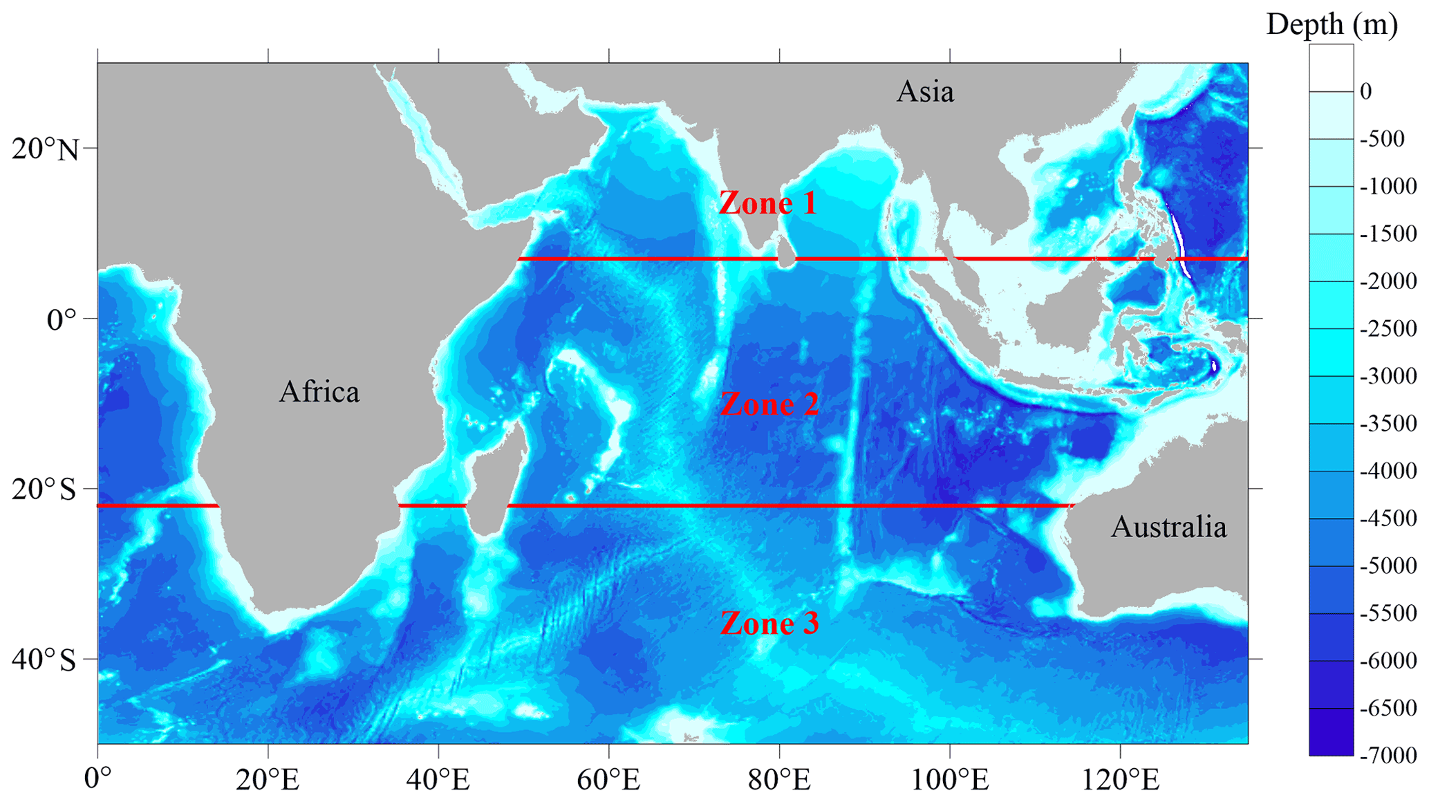
Figure 1 Bathymetric map (color codes in meters) in the Indian Ocean. Red lines (7^∘ N and 22^∘ S) show the zone partition in the present study.

Previous studies, such as Simmons et al. (2004) and Nagai and Hibiya (2015), constructed baroclinic ocean models to compute the energy flux from barotropic tides into internal waves. The Navier–Stokes equations with accurate tidal potential forcing, tidal open boundary conditions and non-hydrostatic approximation were calculated to simulate the generation, development, propagation and dissipation processes of ITs in high-resolution numerical experiments. The induced turbulent mixing coefficients can then be estimated in terms of the local dissipation efficiency, the barotropic to baroclinic energy conversion and the buoyancy frequency. In fact, the estimation of the IT-generated turbulent mixing in these previous studies was implicit. The simulated internal-tide processes will become inaccurate if the temperature and current structure cannot be modeled accurately. On the contrary, we attempt to derive an analytic and explicit expression of the vertical diffusive terms induced by NBSWs and ITs based on the theory of turbulence dynamics as well as surface and internal wave statistics. The mixing schemes introduced in this study will be calculated directly in terms of the parameters of the NBSWs and ITs. The present study provides another way and preliminary attempt to study the mixing processes induced by internal tides. It should be more convenient to improve the simulation further because the mixing schemes are independent of the ocean model.

In this study, the vertical mixing schemes induced by non-breaking surface waves and internal tides are incorporated into the MASNUM ocean circulation model (Han, 2014; Han and Yuan, 2014; Zhuang et al., 2018). The vertical mixing schemes are introduced in Sect. 2. Section 3 describes the model and experiment design. Model results are given in Sect. 4. The relevant discussion is given in Sect. 5, and the conclusions are summarized in Sect. 6.

2 Vertical mixing schemes

2.1 Non-breaking surface-wave-generated turbulent mixing

Previous studies indicated that NBSWs are able to enhance the turbulent mixing in the upper ocean (Babanin and Haus, 2009; Dai et al., 2010; Huang and Qiao, 2010; Qiao et al., 2016). The ability to simulate the SST and MLD can obviously be improved via the incorporation of the related NBSW-induced turbulent mixing schemes into OGCMs (Lin et al., 2006; Xia et al., 2006; Song et al., 2007; Aijaz et al., 2017; Wang et al., 2019). According to Yuan et al. (2011, 2013), Zhuang et al. (2020) expressed the vertical viscosity, B_us, and diffusivity, B_Ts, generated by the non-breaking surface waves (NBSW) as follows:

$$\begin{array}{}\text{(1)}& \left\{\begin{array}{l}{B}_{\mathrm{us}}={\left(\frac{\mathrm{7}}{\mathrm{4}}\right)}^{\frac{\mathrm{1}}{\mathrm{2}}}\cdot h_{\mathrm{sw}}^{\mathrm{2}}\cdot {\left(\sum _{i=\mathrm{1}}^{\mathrm{3}}\sum _{j=\mathrm{1}}^{\mathrm{3}}\left|\frac{\partial u_i}{\partial x_j}\right|\right)}_{\mathrm{sw}}^{\mathrm{2}}/{\left(\sum _{i=\mathrm{1}}^{\mathrm{3}}\sum _{j=\mathrm{1}}^{\mathrm{3}}{\left|\frac{\partial u_i}{\partial x_j}\right|}_{x_{\mathrm{3}}=\mathrm{0}}\right)}_{\mathrm{sw}}\\ B_{\mathrm{Ts}}=\frac{\mathrm{1}}{\mathit{\sigma }}{\left(\frac{\mathrm{7}}{\mathrm{4}}\right)}^{\frac{\mathrm{1}}{\mathrm{2}}}\cdot h_{\mathrm{sw}}^{\mathrm{2}}\cdot {\left(\sum _{i=\mathrm{1}}^{\mathrm{3}}\sum _{j=\mathrm{1}}^{\mathrm{3}}\left|\frac{\partial u_i}{\partial x_j}\right|\right)}_{\mathrm{sw}}^{\mathrm{2}}/{\left(\sum _{i=\mathrm{1}}^{\mathrm{3}}\sum _{j=\mathrm{1}}^{\mathrm{3}}{\left|\frac{\partial u_i}{\partial x_j}\right|}_{x_{\mathrm{3}}=\mathrm{0}}\right)}_{\mathrm{sw}}\end{array}\right.,\end{array}$$

where h_sw is the SWH, and ${\left(\sum _{i=\mathrm{1}}^{\mathrm{3}}\sum _{j=\mathrm{1}}^{\mathrm{3}}\left|\frac{\partial u_i}{\partial x_j}\right|\right)}_{\mathrm{sw}}$ is the averaged velocity shear module of the sea surface waves and can be calculated as

$$\begin{array}{}\text{(2)}& \begin{array}{rl}{\left(\sum _{i=\mathrm{1}}^{\mathrm{3}}\sum _{j=\mathrm{1}}^{\mathrm{3}}\left|{\displaystyle \frac{\partial u_i}{\partial x_j}}\right|\right)}_{\mathrm{sw}}^{\mathrm{2}}& =\mathrm{2}\int \underset{k}{\int }{\mathrm{\Phi }}_{\mathrm{sw}}{K}_{\mathrm{sw}}^{\mathrm{2}}{\mathit{\omega }}_{\mathrm{sw}}^{\mathrm{2}}\\ & \cdot {\displaystyle \frac{\cosh \left[\mathrm{2}{K}_{\mathrm{sw}}(x_{\mathrm{3}}-H)\right]}{{\sinh }^{\mathrm{2}}\left[K_{\mathrm{sw}}\cdot (-H)\right]}}\mathrm{d}{k}_{\mathrm{1}}\mathrm{d}{k}_{\mathrm{2}},\end{array}\end{array}$$

where ω_sw is the surface wave frequency in a typical frequency range: ω_sw>N. N denotes the Brunt–Väisälä frequency, K_sw is the wavenumber and H is the water depth. ${\mathrm{\Phi }}_{\mathrm{sw}}={\mathit{\eta }}_{\mathrm{sw}}\cdot {\mathit{\eta }}_{\mathrm{sw}}^{\ast }$ is the wavenumber spectrum of h_sw, η_sw is the Fourier kernel function of h_sw, i.e., $h_{\mathrm{sw}}=\int \int {\mathit{\eta }}_{\mathrm{sw}}\exp \left\{i\left(k_{\mathrm{1}}x+k_{\mathrm{2}}y-\mathit{\omega }t\right)\right\}\mathrm{d}{k}_{\mathrm{1}}\mathrm{d}{k}_{\mathrm{2}}$ (here the superscript * means the conjugate value), and k₁ and k₂ are the horizontal components of the wavenumber in the x and y directions.

2.2 Mixing induced by surface wave transport flux residue

Apart from NBSWs, the residue of the wave transport flux is also able to contribute to inducing mixing in the ocean circulation through the Reynolds average upon characteristic wavelength scale (Yang et al., 2009, 2019). Yang et al. (2009) proposed a mixing scheme for the wave transport flux residue (WTFR), which has been adopted in OGCMs (Shi et al., 2016; Yu et al., 2020). The results show that the simulated SST and MLD are remarkably improved, especially in summer and in the strong current regions. In tropical cyclone conditions, the performance of the model to simulate ocean response could also be greatly improved if the wave transport flux residue mixing scheme is introduced. The coefficients of the wave transport flux residue mixing are expressed as follows:

$$\begin{array}{}\text{(3)}& \left\{\begin{array}{l}{B}_{\mathrm{SM}\mathrm{1}}=\int \underset{k}{\int }\mathit{\omega }{k}_{\mathrm{1}}E\left(\mathit{k}\right)\frac{\cosh \left[\mathrm{2}K(x_{\mathrm{3}}-H)\right]}{{\sinh }^{\mathrm{2}}\left[K\cdot (-H)\right]}\mathrm{d}{k}_{\mathrm{1}}\mathrm{d}{k}_{\mathrm{2}}\\ B_{\mathrm{SM}\mathrm{2}}=\int \underset{\mathit{k}}{\int }\mathit{\omega }{k}_{\mathrm{2}}E\left(\mathit{k}\right)\frac{\cosh \left[\mathrm{2}K(x_{\mathrm{3}}-H)\right]}{{\sinh }^{\mathrm{2}}\left[K\cdot (-H)\right]}\mathrm{d}{k}_{\mathrm{1}}\mathrm{d}{k}_{\mathrm{2}}\end{array}\right.,\end{array}$$

where E(k) represents the wavenumber spectrum, which can be calculated from the wave spectrum model; other variables are the same as in Eq. (2).

2.3 Internal-tide-generated turbulent mixing

In the stratified ocean interior, ITs are able to provide about half of the mechanical power required for the ocean interior turbulent mixing (Wunsch and Ferrari, 2004; Zhao, 2018; Vic et al., 2019; Whalen et al., 2020). However, current field observations are insufficient for constructing the whole internal-tide map in the IO. Satellite altimetry is able to provide sea surface height (SSH) measurements to observe the global ITs (Ray and Mitchum, 1996). Zhao et al. (2016) presented a method to extract the M₂ ITs by fitting plane waves to satellite altimeter data in individual windows with a size of 160 km × 160 km. In this technique, the least square fitting algorithm is adopted to determine the amplitude and phase of one plane wave. This procedure can be repeated three times to extract the three most dominant M₂ internal waves, superposition of which gives the final internal tidal solution. In this study, the turbulent mixing generated by M₂ semi-diurnal ITs will be derived from the SSH amplitude (Zhao et al., 2016). Other principal tidal constituents will be studied in the future. For simplicity, the mode-1 M₂ ITs, which mainly originate from regions with steep topographic gradients, are considered because the depth-integrated energy and SSH amplitudes of the mode-2 M₂ ITs are much smaller than mode-1 ones (Zhao, 2018).

Yuan et al. (2013) presented a second-order turbulence closure model to estimate the turbulence kinetic energy and dissipation in terms of the velocity shear module of non-breaking waves. The subsurface displacements of ITs, pressure anomalies and currents can be derived from the SSH amplitudes following vertical models (Zhao and Alford, 2009; Wunsch, 2013; Zhao, 2014). The detailed derivation process about the velocity shear module of the internal tide can be found in Appendix A. For the mode-1 M₂ IT, vertical viscosity, B_ui, and diffusivity, B_Ti, generated by the velocity shear can be written as follows:

$$\begin{array}{}\text{(4)}& \left\{\begin{array}{l}{B}_{\mathrm{ui}}={\left(\frac{\mathrm{7}}{\mathrm{4}}\right)}^{\frac{\mathrm{1}}{\mathrm{2}}}\cdot h_{\mathrm{iw}}^{\mathrm{2}}\cdot \frac{{\left(\sum _{i=\mathrm{1}}^{\mathrm{3}}\sum _{j=\mathrm{1}}^{\mathrm{3}}\left|\frac{\partial u_i}{\partial x_j}\right|\right)}_{\mathrm{iw}}^{\mathrm{2}}}{{\left(\sum _{i=\mathrm{1}}^{\mathrm{3}}\sum _{j=\mathrm{1}}^{\mathrm{3}}{\left|\frac{\partial u_i}{\partial x_j}\right|}_{x_{\mathrm{3}}=\mathrm{0}}\right)}_{\mathrm{iw}}}\\ B_{\mathrm{Ti}}=\frac{\mathrm{1}}{\mathit{\sigma }}{\left(\frac{\mathrm{7}}{\mathrm{4}}\right)}^{\frac{\mathrm{1}}{\mathrm{2}}}\cdot h_{\mathrm{iw}}^{\mathrm{2}}\cdot {\frac{{\left(\sum _{i=\mathrm{1}}^{\mathrm{3}}\sum _{j=\mathrm{1}}^{\mathrm{3}}\left|\frac{\partial u_i}{\partial x_j}\right|\right)}_{\mathrm{iw}}^{\mathrm{2}}}{\left(\sum _{i=\mathrm{1}}^{\mathrm{3}}\sum _{j=\mathrm{1}}^{\mathrm{3}}{\left|\frac{\partial u_i}{\partial x_j}\right|}_{x_{\mathrm{3}}=\mathrm{0}}\right)}}_{\mathrm{iw}}\end{array}\right.,\end{array}$$

where h_iw is the SSH amplitude of the mode-1 M₂ IT. ${\left(\sum _{i=\mathrm{1}}^{\mathrm{3}}\sum _{j=\mathrm{1}}^{\mathrm{3}}\left|\frac{\partial u_i}{\partial x_j}\right|\right)}_{\mathrm{iw}}$ is the averaged velocity shear module of the internal tides in a simple monochromatic form and can be calculated based on the unified linear theory under general ocean conditions (Yuan et al., 2011). The expression can be written as

$$\begin{array}{}\text{(5)}& \begin{array}{rl}& {\left(\sum _{i=\mathrm{1}}^{\mathrm{3}}\sum _{j=\mathrm{1}}^{\mathrm{3}}\left|{\displaystyle \frac{\partial u_i}{\partial x_j}}\right|\right)}_{\mathrm{iw}}^{\mathrm{2}}=\mathrm{2}{h}_{\mathrm{iw}}{K}_{\mathrm{iw}}^{\mathrm{2}}{\mathit{\omega }}_{\mathrm{iw}}^{\mathrm{2}}\\ & \cdot {\displaystyle \frac{{\left[{\mathit{\varphi }}^{\mathrm{2}}\left({\mathit{\omega }}_{\mathrm{iw}}\right)-\mathrm{1}\right]}^{\mathrm{2}}{\sin }^{\mathrm{2}}\left[{\int }_{-H}^{x_{\mathrm{3}}}\mathit{\varphi }\left({\mathit{\omega }}_{\mathrm{iw}}\right)K_{\mathrm{iw}}\mathrm{d}{x}_{\mathrm{3}}\right]+\mathrm{2}{\mathit{\varphi }}^{\mathrm{2}}\left({\mathit{\omega }}_{\mathrm{iw}}\right)}{{\sin }^{\mathrm{2}}\left[{\int }_{-H}^{\mathrm{0}}\mathit{\varphi }\left({\mathit{\omega }}_{\mathrm{iw}}\right)K_{\mathrm{iw}}\mathrm{d}{x}_{\mathrm{3}}\right]}},\end{array}\end{array}$$

where

$$\begin{array}{}\text{(6)}& \mathit{\varphi }\left({\mathit{\omega }}_{\mathrm{iw}}\right)=\sqrt{{\displaystyle \frac{N^{\mathrm{2}}-{\mathit{\omega }}_{\mathrm{iw}}^{\mathrm{2}}}{{\mathit{\omega }}_{\mathrm{iw}}^{\mathrm{2}}-f^{\mathrm{2}}}}},\end{array}$$

where ω_iw is the M₂ tidal frequency, and K_iw is the wavenumber. Under the influence of the Earth's rotation, the dispersion relation can be written as

$$\begin{array}{}\text{(7)}& {\mathit{\omega }}_{\mathrm{iw}}^{\mathrm{2}}=K_{\mathrm{iw}}^{\mathrm{2}}{c}_n^{\mathrm{2}}+f^{\mathrm{2}},\end{array}$$

where f is the inertial frequency, and c_n is the eigenvalue speed, which is the phase speed in a non-rotating fluid. The expression can be written as

$$\begin{array}{}\text{(8)}& c_n^{\mathrm{2}}={\left[{\displaystyle \frac{{\int }_{-H}^{\mathrm{0}}N\left(x_{\mathrm{3}}\right)\mathrm{d}{x}_{\mathrm{3}}}{n\mathit{\pi }}}\right]}^{\mathrm{2}},\end{array}$$

where n is the mode number that is set to be 1 here.

2.4 Incorporating the vertical mixing schemes into OGCMs

The effects of the new vertical mixing schemes are introduced into OGCMs. The modified equations can be written as

$$\begin{array}{}\text{(9)}& \left\{\begin{array}{l}\frac{\partial U_i}{\partial t}+U_j\frac{\partial U_i}{\partial x_j}=F+{\mathrm{\Pi }}_U\\ \frac{\partial C}{\partial t}+U_j\frac{\partial C}{\partial x_j}=G+{\mathrm{\Pi }}_C\end{array}\right.,\end{array}$$

where x_j (j=1, 2, 3) represents the x, y and z axes of the Cartesian coordinates, and U_i (i=1, 2, 3) and C denote the mean velocity current components and one of the two tracers including the potential temperature and salinity, respectively. The second terms on the left-hand side of Eq. (9) are the advection ones. F represents the sum of the terms on the right-hand side of the momentum equations including the Coriolis force, pressure gradient force, horizontal diffusion, molecular viscous force and external forcing terms. G represents the sum of the terms on the right-hand side of the tracer equations including horizontal diffusion, molecular diffusivity force, and heat and freshwater flux terms. Π_U and Π_C denote the modified vertical diffusive terms and can be expressed as

$$\begin{array}{}\text{(10)}& \left\{\begin{array}{ll}{\mathrm{\Pi }}_U& =\frac{\partial }{\partial x_{\mathrm{3}}}\left(K_m\frac{\partial U_i}{\partial x_{\mathrm{3}}}\right)+\frac{\partial }{\partial x_{\mathrm{3}}}\left(B_{\mathrm{us}}\frac{\partial U_i}{\partial x_{\mathrm{3}}}\right)\\ & +\left(-B_{\mathrm{SM}\mathrm{1}}\frac{\partial U_i}{\partial x_{\mathrm{1}}}-B_{\mathrm{SM}\mathrm{2}}\frac{\partial U_i}{\partial x_{\mathrm{2}}}\right)+\frac{\partial }{\partial x_{\mathrm{3}}}\left(B_{\mathrm{ui}}\frac{\partial U_i}{\partial x_{\mathrm{3}}}\right)\\ {\mathrm{\Pi }}_C& =\frac{\partial }{\partial x_{\mathrm{3}}}\left(K_h\frac{\partial C}{\partial x_{\mathrm{3}}}\right)+\frac{\partial }{\partial x_{\mathrm{3}}}\left(B_{\mathrm{Ts}}\frac{\partial C}{\partial x_{\mathrm{3}}}\right)\\ & +\left(-B_{\mathrm{SM}\mathrm{1}}\frac{\partial C}{\partial x_{\mathrm{1}}}-B_{\mathrm{SM}\mathrm{2}}\frac{\partial C}{\partial x_{\mathrm{2}}}\right)\\ & +\frac{\partial }{\partial x_{\mathrm{3}}}\left(B_{\mathrm{Ti}}\frac{\partial C}{\partial x_{\mathrm{3}}}\right)\end{array}\right..\end{array}$$

The new vertical diffusive terms Π_U and Π_C can be divided into four parts as shown in Eq. (10). The first term on the right side denotes the original diffusive term, where K_m and K_h are vertical eddy viscosity and diffusivity calculated by the classic Mellor–Yamada 2.5 (M-Y 2.5) scheme (Mellor and Yamada, 1982). The M-Y 2.5 scheme is a level-2.5 turbulence model based on the modification of the material derivative and diffusive terms. The mixing coefficients K_m and K_h can be calculated as the turbulence characteristics ql multiplied by a stability function associated with the Richardson number, where q represents the turbulent fluctuation velocity, $q^{\mathrm{2}}/\mathrm{2}$ is the turbulence kinetic energy and l is the mixing length scale. The turbulence kinetic energy $q^{\mathrm{2}}/\mathrm{2}$ can be estimated from the local shear production, buoyancy and dissipation based on the q²−q²l closure equations in the atmospheric boundary. Actually, the M-Y 2.5 scheme was proposed based on the assumption of a rigid surface and did not consider the effects of surface and internal waves (Qiao et al., 2004; Huang and Qiao, 2010; Huang et al., 2011), which is regarded as one of the major reasons for the insufficient mixing in the upper-ocean simulation. The remaining terms represent the new diffusive terms generated by surface waves and internal tides, which are described in Sect. 2.1–2.3.

3 Model description and numerical experiment design

3.1 Ocean circulation model

The three-dimensional MASNUM ocean circulation model (Han and Yuan, 2014; Zhuang et al., 2018) is used to evaluate the effects of NBSW- and IT-generated turbulent mixing and WTFR-induced mixing. The two-level single-step Eulerian forward–backward time-differencing scheme and the σ–Z–σ hybrid vertical coordinate are adopted in the MASNUM ocean model. The forward–backward scheme with a spatial smoothing method should be superior to the leapfrog scheme because of more stability and more computational efficiency (Han, 2014). Han (2014) and Han and Yuan (2014) have tested the modeling ability of the MASNUM model compared with the POM. The results showed that the MASNUM model could produce quite identical simulation results as the existing models with only half the computer cost.

The model domain is in an area of 50^∘ S–30^∘ N, 0–135^∘ E (Fig. 1) with a horizontal resolution of 1^∘ $/$ 6 by 1^∘ $/$ 6. 5 surface σ layers and 31 intermediate Z layers. Three bottom σ layers are used in the vertical direction in order to obtain the vertical grid spacing with a high resolution in the upper ocean. The topography of the model is downsampled from the global General Bathymetric Chart of the Oceans 2008 (GEBCO_08) with a resolution of 1 by 1. The minimum depth is set to 5 m. The maximum depth is set to 5000 m, avoiding artificial influences at deep-water depths. The topography has been smoothed using the dual-step five-point-involved spatial smoothing method (Han, 2014) to make the calculation more stable. The topographic gradients were not considered to be a key factor in this study because the climatological experiments in this study are inappropriate to directly simulate the ITs.

The initial temperature and salinity are interpolated based on annual mean Levitus94 data (Levitus and Boyer, 1994; Levitus et al., 1994) with the horizontal resolution of 1^∘ by 1^∘ and 33 vertical layers. The initial velocities are set to 0. The gravity-wave radiation conditions (Chapman, 1985) were used as the lateral boundary conditions, which are very important for basin-scale modeling in this study. The simulated variables, including velocities, temperature, salinity and SSH, on the lateral boundary grids are calculated in an explicit numerical form. In the explicit form, the values of the related variables obtained from the daily global climatologic model results by the MASNUM model with the horizontal resolution of 1^∘ $/$ 2 by 1^∘ $/$ 2 are also used. The lateral boundary conditions are time-dependent with an updating period of 1 d. The surface forcing including the momentum, heat and wind stress fluxes is calculated from the monthly mean surface fields of the National Centers for Environmental Prediction/National Center for Atmospheric Research (NCEP/NCAR) reanalysis dataset with the horizontal resolution of 1^∘ $/$ 4 by 1^∘ $/$ 4. We calculated the multiyear monthly mean surface forcing results based on the time series of the NCEP/NCAR data from 1948 to 2021. Then the model is driven by the monthly mean surface forcing results, which repeats in every climatologic year. The time step size of the barotropic mode is set to 30 s, while that of the baroclinic mode is 900 s. The model is integrated from the quiescent state for 10 climatological years. The simulated results in the last 1 year are compared with the monthly World Ocean Atlas 2013 (WOA13) and the Ocean Surface Current Analyses Real-time (OSCAR) climatologic data, which can be regarded as the true solution of the climatological numerical experiments.

It is worth noting that the time interval of 10 years should be appropriate for ocean simulation from the quiescent state to a relatively stable circulation background. The average kinetic energy, which can be regarded as a model stability index, fluctuated obviously in the first 2 years, then became stable gradually in the third year and was completely steady from the fourth to the 10th year. The conclusion is similar to many previous studies (e.g., Xia et al., 2006; Qiao et al., 2010; Han, 2014; Yu et al., 2020).

3.2 Wave spectrum model

The MASNUM wave spectrum model (Yuan et al., 1991, 1992; Yang et al., 2019) is used to simulate the parameters of surface waves in the IO. The energy-balanced equations are solved in the model based on the wavenumber spectrum space. The characteristic inlaid scheme is adopted for the wave energy propagation to improve the original wave model (Yuan et al., 1992). The wave model has been validated by observations (Yu et al., 1997) and widely accepted in ocean engineering and numerical simulation (e.g., Qiao et al., 1999; Xia et al., 2006; Qiao et al., 2010; Shi et al., 2016; Yang et al., 2019; Yu et al., 2020; Sun et al., 2021). The results showed that the simulated SWH and mean wave period are consistent with satellite observations.

The model domain, resolution, topography and surface wind stress flux data are consistent with those in the MASNUM ocean circulation model. The boundary conditions are from the JONSWAP spectrum (Hasselmann et al., 1973). The wave model is integrated from the quiescent state for 10 climatological years with the same period as the ocean circulation model. Actually, the configuration of the wave model is simpler than the OGCM, and the model design in this study is almost the same as that in Xia et al. (2006) and Qiao et al. (2010). Therefore, we believe that the experiment using the MASNUM wave model is able to characterize the spatial pattern and variation of surface waves in the IO.

The wave spectrum E(k) is calculated from the MASNUM wave model, and then ω_sw, K_sw and h_sw can be estimated. Thus, the new mixing coefficients including B_us, B_Ts, B_SM1, B_SM2, B_ui and B_Ti are calculated directly from Eqs. (1)–(4).

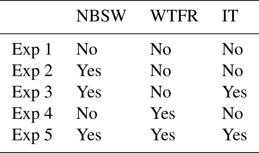
3.3 Experimental design

To assess the effects of the NBSW, WTFR and IT on the vertical mixing and simulated thermal structure in the upper ocean, five experiments (Table 1) are denoted as Exp 1–5 and designed as follows.

Exp 1 (benchmark experiment). The model is integrated with the classic M-Y 2.5 turbulence closure model (Mellor and Yamada, 1982), which is broadly used in OGCMs.

Exp 2. Same as Exp 1, except with the classic M-Y 2.5 scheme and the NBSW-generated turbulent mixing scheme. This experiment is designed to evaluate the effect of NBSWs.

Exp 3. Same as Exp 1, except with the classic M-Y 2.5 scheme and the NBSW- and IT-generated turbulent mixing schemes. This experiment is designed to evaluate the effects of NBSWs and ITs. The experiment with the M-Y 2.5 scheme and the IT-generated turbulent mixing scheme (Exp 3.5) is omitted in this study because the deviation of the temperature between Exp 1 and Exp 3.5 is too small. The possible reason is that ITs are often considered to enhance vertical mixing in the ocean interior from the thermocline to abyssal regions (Munk and Wunsch, 1998; Wunsch and Ferrari, 2004; Kunze et al., 2006); therefore, it could be insufficient for the incorporation of only ITs into the M-Y 2.5 scheme to draw warmer water from the surface into the interior. This implies that only the IT is unable to improve the upper-ocean simulation.

Exp 4. Same as Exp 1, except with the classic M-Y 2.5 scheme and the WTFR-induced mixing scheme. Comparisons between Exp 2 and Exp 4 are implemented to evaluate the two mechanisms through which the surface waves affect the upper-ocean vertical mixing.

Exp 5. Same as Exp 1, except with the classic M-Y 2.5 scheme, NBSW- and IT-generated turbulent mixing, and the WTFR-induced mixing scheme. This experiment is designed to evaluate the effects of NBSWs, ITs and WTFR.

Table 1 Numerical experiment design.

It is worth noting that the climatological experiments, which should be regarded as the multiyear mean simulation, are designed in this study, so it is inappropriate for the simulated results to be compared with the Argo data because there should be a considerable difference between the climatologic data and real-time in situ observations. The WOA13 data, which represent the multiyear (1955–2012) mean results, and the multiyear (1993–2021) mean OSCAR data will be a good choice to evaluate the ocean climatological modeling.

4 Results

In this section, the comparable results for the climatological temperature construction in the upper ocean are used to assess the effects of NBSWs, ITs, and WTFR on vertical mixing.

4.1 Comparison of vertical diffusive terms

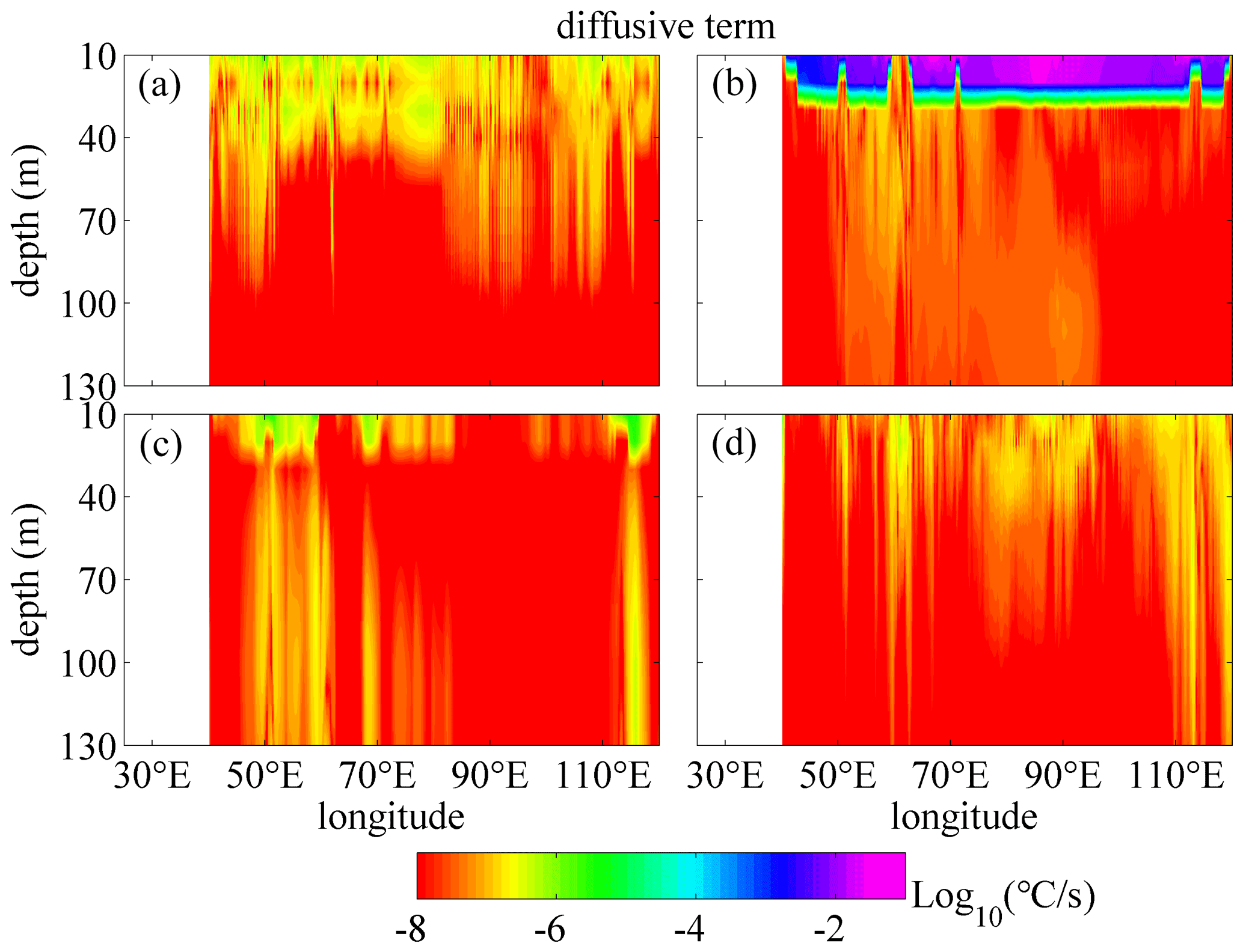
As a typical example, the vertical distribution of the monthly mean vertical temperature diffusive terms in logarithmic scale along the zonal transect of 10.5^∘ S in January and July is shown in Figs. 2 and 3. As expressed in Eq. (10), the following are presented: the calculated vertical diffusive term based on the M-Y 2.5 scheme, which is written as $\frac{\partial }{\partial x_{\mathrm{3}}}\left(K_h\frac{\partial T}{\partial x_{\mathrm{3}}}\right)$ (KHT for short) and calculated from Exp 1; the NBSW-generated turbulent mixing scheme, which is written as $\frac{\partial }{\partial x_{\mathrm{3}}}\left(B_{\mathrm{Ts}}\frac{\partial T}{\partial x_{\mathrm{3}}}\right)$ (BTST) and calculated from Exp 2; the IT-generated turbulent mixing scheme, which is written as $\frac{\partial }{\partial x_{\mathrm{3}}}\left(B_{\mathrm{Ti}}\frac{\partial T}{\partial x_{\mathrm{3}}}\right)$ (BTIT) and calculated from Exp 3; and the WTFR-induced mixing scheme, which is written as $-B_{\mathrm{SM}\mathrm{1}}\frac{\partial T}{\partial x_{\mathrm{1}}}-B_{\mathrm{SM}\mathrm{2}}\frac{\partial T}{\partial x_{\mathrm{2}}}$ (BSMT) and calculated from Exp 4. The BTIT can be calculated independently as part of the diffusive terms in Exp 3. Figures 2 and 3 show the comparisons among these diffusive terms along 10.5^∘ S, which is a typical transect to show the difference, in January and July. There are two reasons for the choice of the 10.5^∘ S transect. Firstly, the Madagascar–Mascarene regions (0–25^∘ S in the western Indian Ocean) are considered to be a hot spot for the generation of semi-diurnal ITs (Zhao et al., 2016). Both NBSWs and ITs should grow fully and become large enough for the comparison of the diffusive terms. Secondly, the 10.5^∘ S transect is typical to show the spatial pattern among the diffusion terms because of the stronger surface waves and ITs (Kumar et al., 2013; Zhao et al., 2016; Ansong et al., 2017).

One can see that all of the terms decay with the depth below the sea surface. In January, BTST is $>{\mathrm{10}}^{-\mathrm{2}}$ ^∘C s⁻¹ in the upper 30 m layer of most regions, the values of which are too high to show in Figs. 2b and 3b, and obviously greater than other terms, implying that the NBSW-generated turbulent mixing is dominant in layers with depths less than 30 m. Similar to BTST, BSMT (Fig. 2d) is also induced by NBSW and directly generated by the surface wave orbital velocity, but the values are about 4 to 6 orders smaller than those of BTST. However, in July, BSMT may affect greater depths than BTST and KHT, especially in some regions with large topographic relief. In the ocean interior with depths from 40 to 130 m, BTIT (Fig. 2c) is about 10^−6 ∘C s⁻¹ and significantly higher than the other three terms in some regions such as the eastern Atlantic (5–10^∘ E), the western Indian Ocean (50–70^∘ E) and the western Pacific (122–125^∘ E) because of the effects of the IT. It is worth noting that the vertical distribution of the eddy diffusivity (K_h, B_Ts and B_Ti) is very similar to the diffusive terms. Especially in January, B_Ts is the largest in the upper 30 m layers and B_Ti is generally larger in the ocean interior with depth deeper than about 40 m. K_h and B_Ts decay with depth below the sea surface, and the delay rate of B_Ts is obviously slower than K_h, so B_Ts is larger than K_h in the ocean interior. The high-value layers ($>{\mathrm{10}}^{-\mathrm{5}}$ m² s⁻¹) of K_h are as thin as about 20 m in January and up to about 80 m partially in July, while the high-value layers of the B_Ts are generally about 70–100 m in both January and July. When the depth is larger than 40 m, the value of B_Ti appears to be about 10⁻⁵–10⁻³ m² s⁻¹.

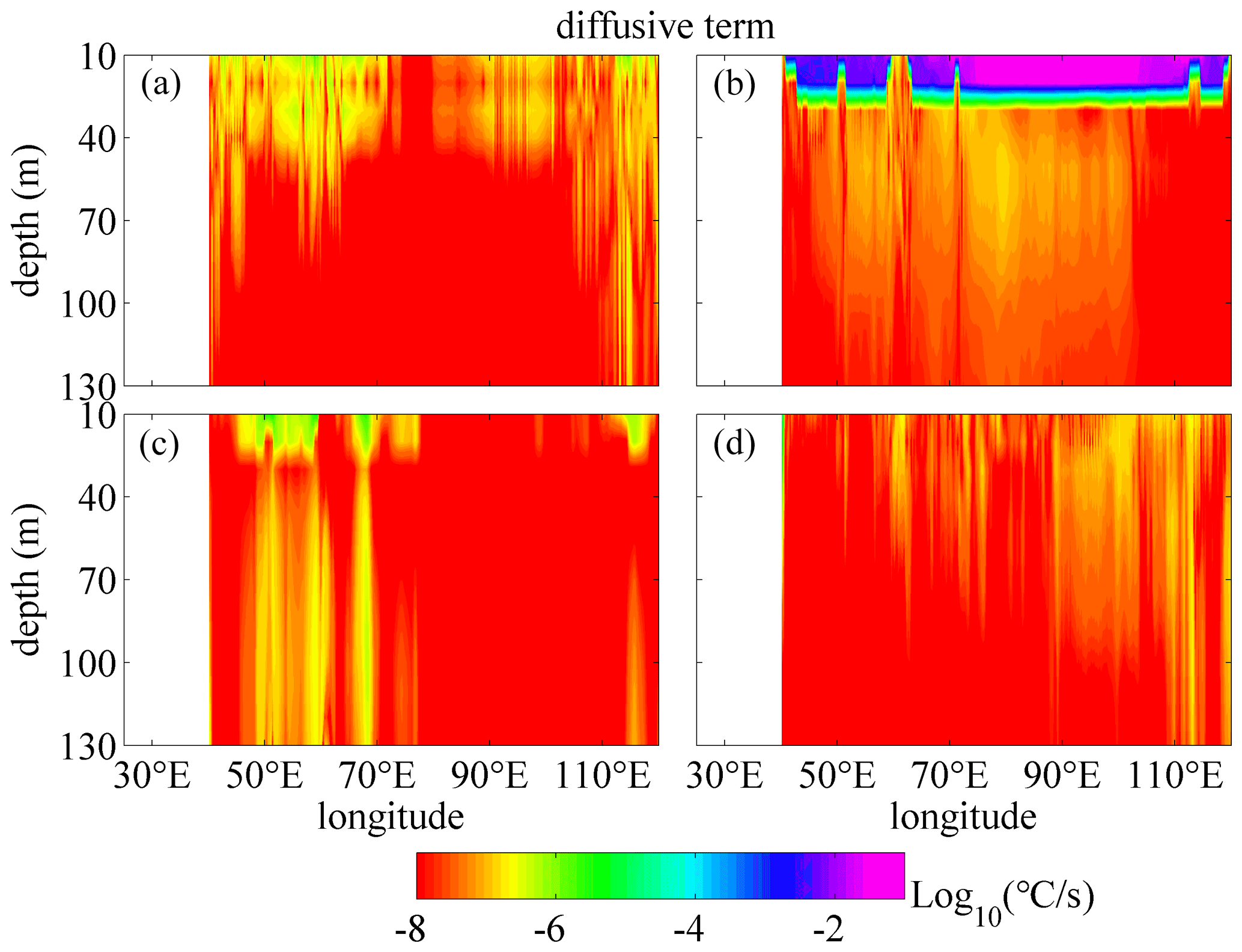
Figure 2 Vertical profiles of the monthly mean vertical temperature diffusive terms in logarithmic scale along 10.5^∘ S in January, including the diffusive term based on the M-Y 2.5 scheme (a), the NBSW-generated turbulent mixing scheme (b), the IT-generated turbulent mixing scheme (c) and the WTFR-induced mixing scheme (d). Deep yellow areas correspond to land.

Figure 3 The same as Fig. 2, but in July.

4.2 Effects on simulation of the vertical temperature structure

The climatologic experiments are designed in this study because of the NCEP monthly climatological sea surface flux forcing fields and the daily global climatological lateral boundary conditions in the simulation, so the WOA13 monthly climatology data can be used in comparisons as a reference.

Figures 4–7 show the comparisons of the upper-ocean temperature vertical structure between the WOA13 data and the model results of the five experiments along transects of 30.5^∘ S and 7.5^∘ N, corresponding to SIO and north of the equatorial Indian Ocean (EIO), in January and July. In the Southern Hemisphere, the 30.5^∘ S transect is typical to show the effects of the three schemes on the temperature modeling. The temperature structure along 10.5^∘ S, which is used to show the comparison of the diffusive terms in Sect. 4.1, is omitted here because there is a non-ignorable difference between the WOA13 data and the simulation results, especially in the eastern Indian Ocean, and the effects of the NBSW in the tropical area are relatively non-obvious, which is regarded as a long-standing issue (Qiao et al., 2010; Zhuang et al., 2020). In the Northern Hemisphere, the temperature structure along the 7.5^∘ N transect, which is located in the south of the Arabian Sea and Bay of Bengal and regarded to be representative for modeling evaluation, is discussed. One can see that the difference by subtracting the monthly mean results of Exp 1 from the monthly WOA13 data is the largest among the five experiments along the two transects in January and July. In the ocean interior, the temperature of Exp 1 is extremely lower than the WOA13 data, which implies that less surface water is transferred into the layers with depths from 30 to 100 m in Exp 1 because of the insufficient vertical mixing process simulated by the classic M-Y 2.5 scheme. Compared with Exp 1, the difference for Exp 2 decreases remarkably because the NBSW strengthens the vertical mixing and improves the upper-ocean simulation, which has been proved many times by previous studies (Lin et al., 2006; Huang et al., 2011; Qiao et al., 2016; Zhuang et al., 2020).

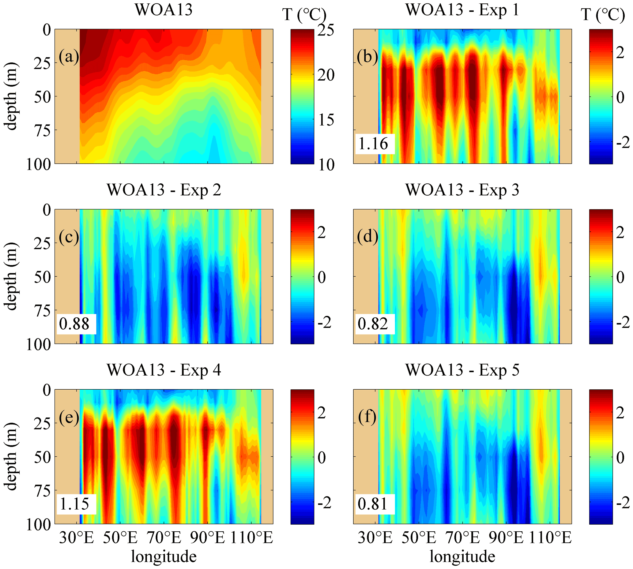
Figure 4 The vertical temperature profiles along 30.5^∘ S in January. (a) The temperature structure from the monthly WOA13 data (units: degrees). (b–f) The difference of the temperature calculated by subtracting the monthly mean results simulated in Exp 1–Exp 5 from the monthly WOA13 data, respectively. The RMSE of the temperature in the upper 100 m regions between the WOA13 data and the model results are given. Deep yellow areas correspond to land.

Figure 5 The same as Fig. 4, but in July.

Figure 6 The same as Fig. 4, but along 7.5^∘ N.

Figure 7 The same as Fig. 4, but along 7.5^∘ N and in July.

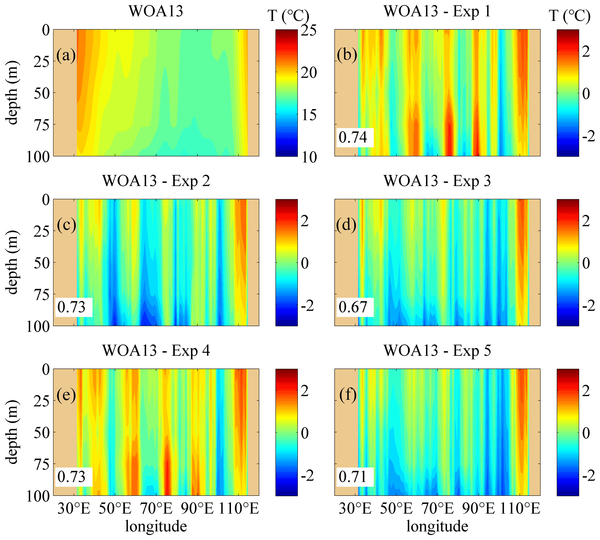
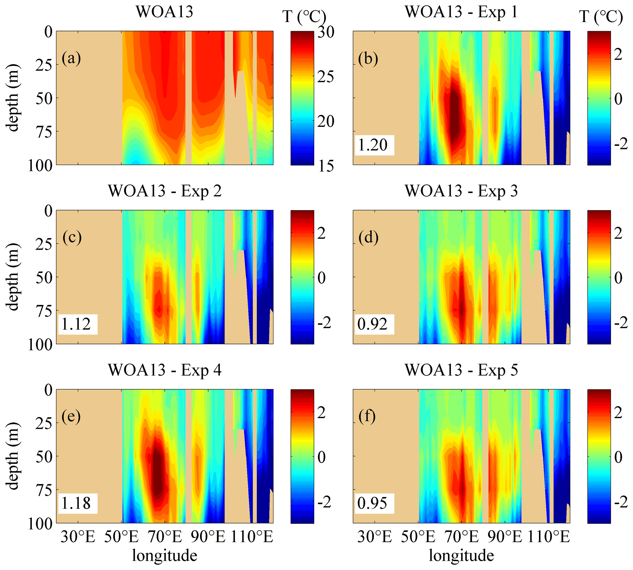
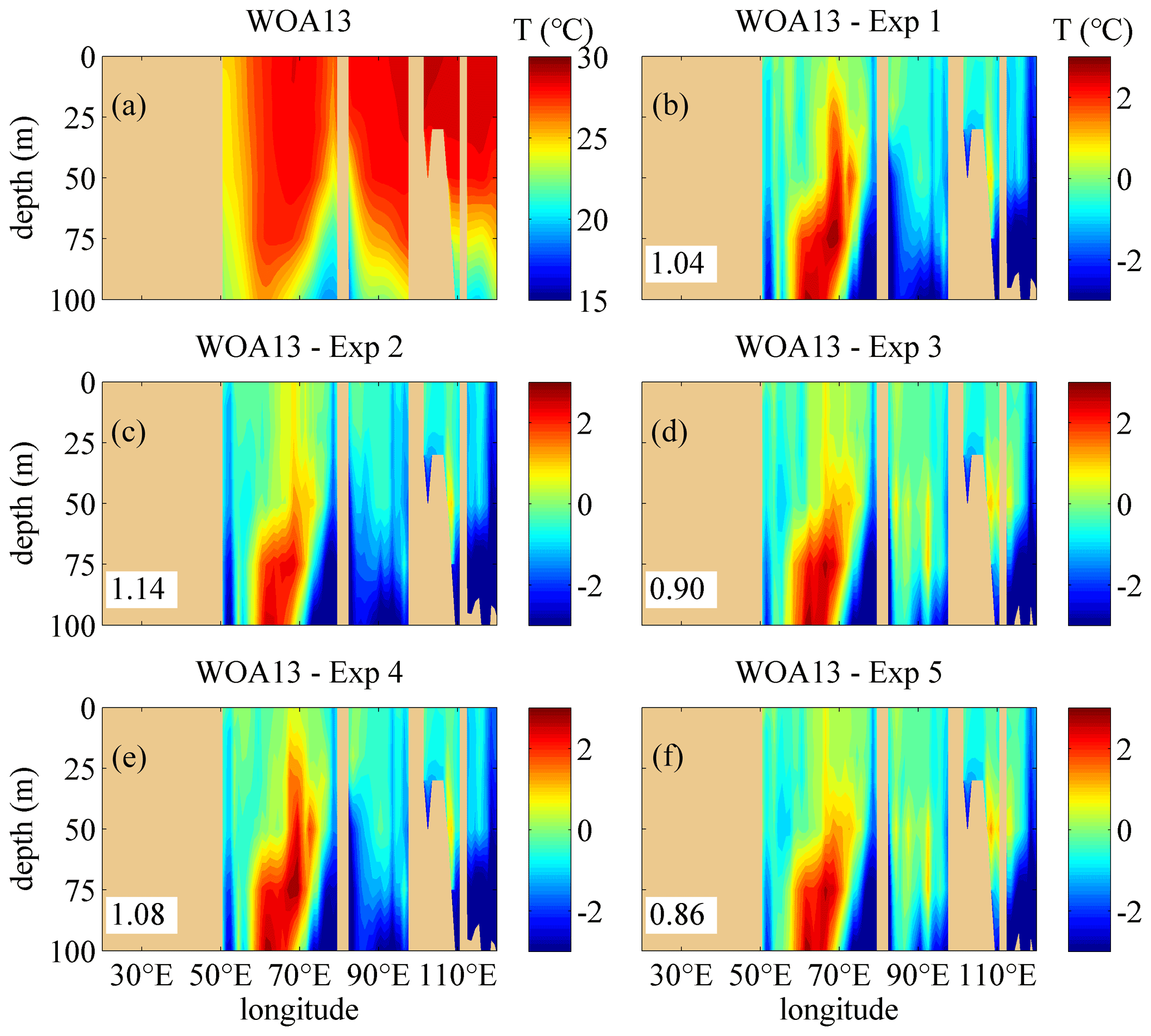
The difference for Exp 3 is much smaller than that of Exp 1 and Exp 2 because of the incorporation of the IT-generated turbulent mixing, especially in layers with depths between 20 and 50 m. This implies that the IT strengthens the vertical mixing of the ocean interior and improves the simulation further. It is worth noting that the experiment with the classic M-Y 2.5 scheme and the IT-generated turbulent mixing scheme is omitted; the reason is that the results have not been improved if only the IT-generated turbulent mixing is incorporated because the simulated surface mixing is insufficient and even deteriorated in some regions because colder water will be drawn from the lower layers with depths deeper than 100 m into the upper ocean.

However, the simulation is slightly improved in Exp 4 compared with Exp 1 because the BSMT, which is induced by the WTFR, is remarkably smaller than the BTW, so the WTFR-induced mixing is too insufficient to significantly improve simulating the upper-ocean temperature structure. Similarly, there is less difference between Exp 3 and Exp 5, implying that the effects of the WTFR on enhancing vertical mixing are much weaker than the NBSW in the surface layers and the IT in the ocean interior.

In Exp 1, the simulated temperature along 30.5^∘ S is cooler than the WOA13 data, while the temperature bias becomes reversed with similar magnitude in Exp 2 and Exp 3. The reason should be that the multiyear monthly mean surface forcing fields, on one hand, were smaller than the actual values, which leads to insufficient heat transfer from the atmosphere to the ocean. After 10 climatologic years of modeling, the temperature in the ocean interior became obviously cooler than the WOA13 data. On the other hand, NBSWs and ITs enhanced the vertical mixing as well as the heat transfer, so more heat entered the ocean interior and the SST became cooler. Additionally, the Haney equation (Haney, 1971), which improves the large-scale thermal coupling of the ocean and atmosphere, is used to modify the surface heat flux. However, a disadvantage of the Haney modifying method is the destruction of the heat balance, so solar radiation will continuously increase in the ocean surface. Therefore, the accumulation of heat during the 10-year modeling will make the temperature bias in Exp 2 and Exp 3 reversed, with similar magnitude in Exp 1. Furthermore, the temperature from the annual mean Levitus94 data, which are used as the initial fields, is cooler by about 3^∘ than that from the WOA13 data in the Antarctic Circumpolar Current (ACC) region from the surface to 200 m depth and warmer by about 0.5^∘ in the NIO and tropics when the depth is deeper than 200 m. This should make the simulated temperature cooler than the WOA13 data in the SIO and become warmer in the NIO and the tropics. The improvement of NBSWs and ITs in the temperature simulation is obvious because of the smaller errors in Exp 2 and Exp 3, although the difference of the temperature bias between Exp 1 and Exp 2–3 is substantial.

Figure 8 shows the monthly variability of the root mean square errors (RMSEs) of the temperature in the upper 100 m layers between the WOA13 data and the model results. Actually, the RMSEs are calculated based on the simulated temperature only in the whole IO (the regions outside the IO have been removed) as the following expression:

$$\begin{array}{}\text{(11)}& \mathrm{RMSE}=\sqrt{{\displaystyle \frac{\sum _{i=\mathrm{1}}^{\mathrm{im}}\sum _{j=\mathrm{1}}^{\mathrm{jm}}\sum _{k=\mathrm{1}}^{\mathrm{ks}}{\left(t_{mi,j,k}-t_{\mathrm{w}i,j,k}\right)}^{\mathrm{2}}}{\mathrm{im}\times \mathrm{jm}\times \mathrm{ks}}}},\end{array}$$

where t_m and t_w represent the model results and the WOA13 data for the monthly mean temperature, and im, jm and ks mean the number of grids in the whole IO in the horizontal and vertical directions. The RMSE can be regarded as a spatial average deviation of the three-dimensional temperature fields. Therefore, the RMSE should be statistically robust because the calculated result is unique if the spatial range of the temperature field is determined.

The study area is divided into three zones (Zones 1–3 marked in Fig. 1). The zone partition of the IO in this study is designed based on previous studies and the dynamic patterns of the IO. On one hand, previous studies (Talley et al., 2011; Kumar et al., 2013, 2018) showed different zone partitioning criteria, which often included the NIO, SIO and tropical regions. On the other hand, the principal upper-ocean flow regimes of the IO are the subtropical gyre of the SIO and the monsoonally forced circulation of the tropics and NIO. All effects of the Indonesian throughflow (ITF) should also be considered. Taking the above factors into account, the whole IO was divided into three parts. Zone 1 represents the NIO including the Arabian Sea and the Bay of Bengal. Zone 2 represents the tropics and subtropical regions in the SIO with all effects of the subtropical gyre and the ITF. Zone 3 represents the region in the south of Zone 2 in the SIO. In Zone 2, there is a complete cyclonic circulation system between the Equator and 20^∘ S, consisting of the westward South Equatorial Current on the south side, the eastward South Equatorial Countercurrent on the north side, the northward East African Coastal Current and the ITF. The effects of the M₂ internal tides, which are generated in the northern regions around Madagascar, are produced throughout the whole west region in Zone 2.

In Zone 1, the RMSEs for Exp 2 are smaller than for Exp 1 in all of the months, indicating the improvement of the NBSW in the upper-ocean simulation in the NIO. Compared with Exp 2, the RMSEs for Exp 3 are smaller in most of the months except November, December and January. This implies that the IT enhances vertical mixing and improves the simulation further. The possible reason for few effects of the IT from November to January is that, on one hand, the mixed layer depths in the NIO are relatively shallower in boreal winter so that the averaged velocity shear module of the internal tides is smaller and the IT-induced mixing is weaker; on the other hand, the strength of the surface waves is more intensive, so the NBSW-induced mixing is relatively sufficient. The largest declines occurred in May, when the RMSE decreased 14.0 % from 1.72^∘ (Exp 1) to 1.49^∘ (Exp 2) and 19.1 % from 1.72^∘ (Exp 1) to 1.40^∘ (Exp 3).

In Zone 2, the NBSW is ineffective because the RMSEs for Exp 2 are almost equal to, or even larger than, those for Exp 1. This is a long-standing issue about the trivial effects of the NBSW in the tropical area (Qiao et al., 2010; Zhuang et al., 2020), implying that only the NBSW should not be enough to improve the tropical simulation. To solve this issue, coupled atmosphere–wave–ocean–ice modeling is one solution (Song et al., 2012; Wang et al., 2019). Another way is incorporation of the additional mechanism into OGCMs, such as the IT-generated turbulent mixing added in Exp 3 and Exp 5. The RMSEs for Exp 3 are obviously smaller than for Exp 1 and Exp 2 in the whole climatologic year except March, implying that the combination of the NBSW and the IT is able to improve the simulation of the temperature structure in the tropical area. Additionally, the RMSEs in Zone 2 are smaller than in Zones 1 and 3 on the whole, and the RMSEs in Zone 2 for Exp 3 and Exp 5 are even less than 0.9^∘ in half of the climatologic year, indicating much accurate simulation in the tropical area.

In Zone 3, the results are similar to those in Zone 1. The RMSEs for Exp 2 are smaller than for Exp 1 in most months, and the RMSEs for Exp 3 are the smallest ones among the first three experiments. The largest declines occurred in January, when the RMSE decreases 20.8 % from 1.50^∘ (Exp 1) to 1.18^∘ (Exp 2) and 25.7 % from 1.50^∘ (Exp 1) to 1.11^∘ (Exp 3). The situation also indicates significant improvements from the combination of the NBSW and IT in simulating the upper-ocean temperature structure.

Furthermore, in Zones 1–3, the effects of WTFR are much weaker and similar to those in Figs. 4–7 because the RMSEs for Exp 4 and 5 are almost equal to, and even larger than, those for Exp 1 and 3. The possible reason is that the values of the WTFR-induced diffusion terms are about 4 to 6 orders smaller than NBSW, which is too low to enhance vertical mixing, especially in the surface layers.

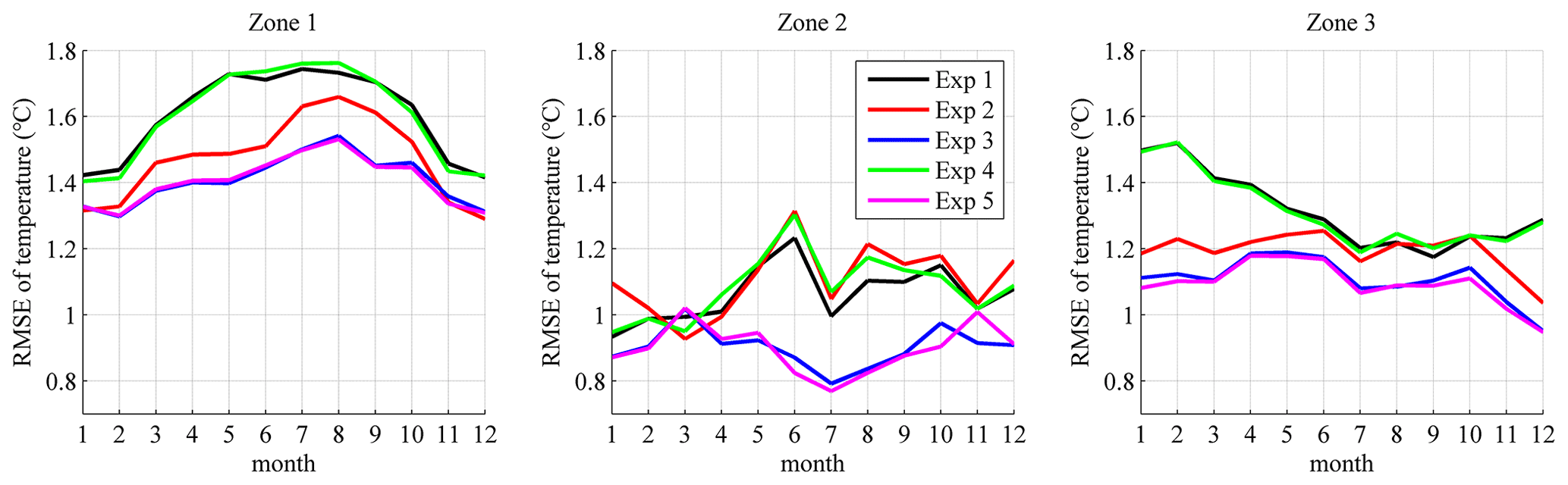
Figure 8 Variation of the RMSE of temperature between the simulated monthly mean results in the five experiments and the monthly WOA13 data in Zones 1–3 (shown in Fig. 1).

The thermal structure in the regions with depths from 100 to 300 m are also compared with the WOA13 data. The simulated temperature is generally cooler than the WOA13 data along 30.5^∘ S at depths between 100 and 300 m, while it is dramatically warmer along 7.5^∘ N. The distribution pattern of the simulated temperature in the ocean interior (from 100 to 300 m or deeper) seems cooler in SIO and warmer in NIO and the tropics. One of the reasons is that the Haney equation (Haney, 1971) is used to modify the climatologic surface heat flux and brings excessive heat into the ocean interior in the simulation. Some more accurate surface forcing data with higher resolution will be used in future simulations.

Furthermore, the intermediate and deep-water masses in the IO are often effected by the Southern Ocean, including Antarctic Intermediate Water, Circumpolar Deep Water and North Atlantic Deep Water. These cooler water masses are carried by the meridional overturning circulation into the IO throughout the south of the South Equatorial Current in the subtropical Indian Ocean (Talley et al., 2011), but the situation did not appear in the simulated current fields. Therefore, another important reason should be that it is hard to accurately simulate the meridional overturning circulation in the present experiments, especially the meridional transport of heat. This makes the simulated temperature cooler or warmer than the WOA13 data along 30.5^∘ S and 7.5^∘ N when the depth is deeper than about 100 m.

In addition, it is worth noting that the initialization design is also important for ocean modeling. The comparison between the annual mean temperature between the Levitus94 and WOA13 data shows that the temperature from the Levitus94 data is obviously cooler than that from the WOA13 data in the ACC regions (45–75^∘ E, 35–50^∘ S), while it is generally warmer in the whole IO at depths from 200 to 500 m. The WOA13 data contain more mesoscale information than the Levitus94 data. Therefore, the inaccurate initial field could also be one of the reasons why the simulated temperature in the ocean interior is different from the WOA13 data. A series of high-resolution real-time numerical experiments for the circulation in the IO will be carried out to examine the influence of different initial fields, parameterization schemes, surface fluxes and open boundary conditions in the future. It is worth noting that the detailed analysis of the deep ocean is omitted here because the vertical mixing in the upper ocean (0–100 m) is the main focus of this study.

Lozovatsky et al. (2022) demonstrated that internal wave instabilities appear to be a dominant mechanism for generating energetic mixing based on an analysis of in situ observations of the turbulent kinetic energy dissipation rate and buoyancy frequency profiles. Actually, designing a universal and flexible IT-induced mixing scheme for ocean modeling based on in situ observations still needs a lot of work. The three schemes introduced in this study are just preliminary research on the contribution of upper-ocean vertical mixing.

The thermocline structure, which is normally defined as the depth of the 20^∘ isothermal (Z20), can affect SST variability via vertical water exchange and thereby modulate air–sea interaction events (Talley et al., 2011). Vertical displacements of the thermocline depth at the equatorial region are regarded as one of the distinctive features in the IO. Because of the weak westerly at the Equator, the IO shows a deeper and reversed slope of Z20 compared to its counterpart in the Pacific Ocean. Analysis of the mean state thermocline structure is very important because the thermocline variability is related to the Indian Ocean Dipole, ITF and El Niño–Southern Oscillation at the interannual timescale according to previous studies (e.g., Chambers et al., 1999; Gordon et al., 2003; Liu et al., 2017). Figure 9 shows the variation of the Z20 depths along the Equator in January and July. As another indicator of the thermal structure in the upper 100 m layers, the depths of the 26^∘ isothermal (Z26) are also plotted in Fig. 9a and b. The RMSEs of the Z20 and Z26 depths are calculated and plotted in Fig. 9c and d.

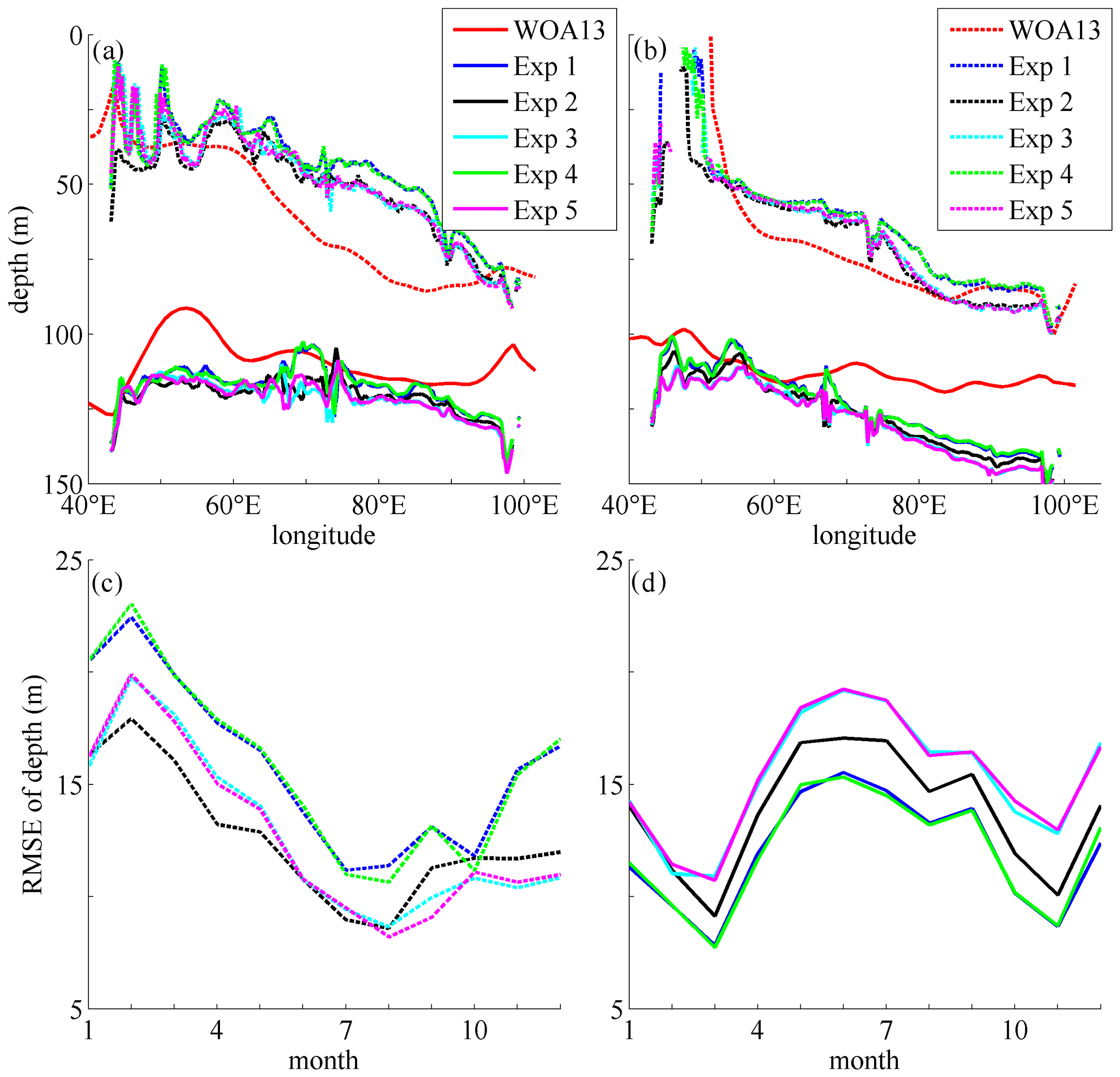
Figure 9 The comparison of Z20 and Z26 depths along the Equator from the WOA13 data and the model results. (a, b) The Z20 (solid curves) and Z26 (dashed curves) depths from the WOA13 data and model results (Exp 1–Exp 5) in January and July, respectively. The RMSEs of the Z26 (c) and Z20 (d) depths along the Equator in the whole climatologic year are also plotted.

From Fig. 9 one can see that the Z20 and Z26 depths are both shallow in the west and deep in the east. The simulations of the thermal structure in the five experiments depict this pattern successfully, but there is still an obvious difference between the WOA13 data and the results, especially in the east regions in January for Z26 depths and in July for Z20 depths. One of the main reasons should be that the ITF may be simulated inaccurately because of inaccurate topography in the Indonesian regions and the open boundary conditions. The accurate simulation of the ITF should be a difficult issue because of the complicated topography and ocean–atmosphere interaction in the Indonesian Archipelago. Many OGCMs are incapable of reproducing the patterns of the ITF (Nagai et al., 2017; Santoso et al., 2022). Another reason is that this area is full of eddies produced by horizontal velocity shear, but our ocean model still lacks an accurate and reasonable parameterization of eddy-induced mixing, which needs more future work. For Z26 depths, the RMSEs for Exp 1 and Exp 4 are the largest in almost all of the months; this implies that the WTFR-induced mixing has little effect on the modeling, which is consistent with the comparison results above (Figs. 4–8). The NBSW- and IT-generated turbulence mixing can improve the simulated thermal structure as two of the key factors because of the smallest RMSEs (from February to July for Exp 2 and from August to January for Exp 3 and Exp 5). For Z20 depths, the NBSW and the IT have negative effects on the modeling because the RMSEs for Exp 2–Exp 5 are obviously larger than those for Exp 1. The reason is that the Z20 isothermal simulated in Exp 1 is generally deeper than the WOA13 data because the simulated temperature in the regions with depths from 130 to 200 m is warmer than the WOA13 data, and the enhanced vertical mixing induced by the NBSW and the IT will make the Z20 isothermal deepen further and deviate more from the WOA13 data (solid curves in Fig. 9a and b). Therefore, more optimization and improvement of the experimental design will be implemented in future work to make the simulated results more accurate.

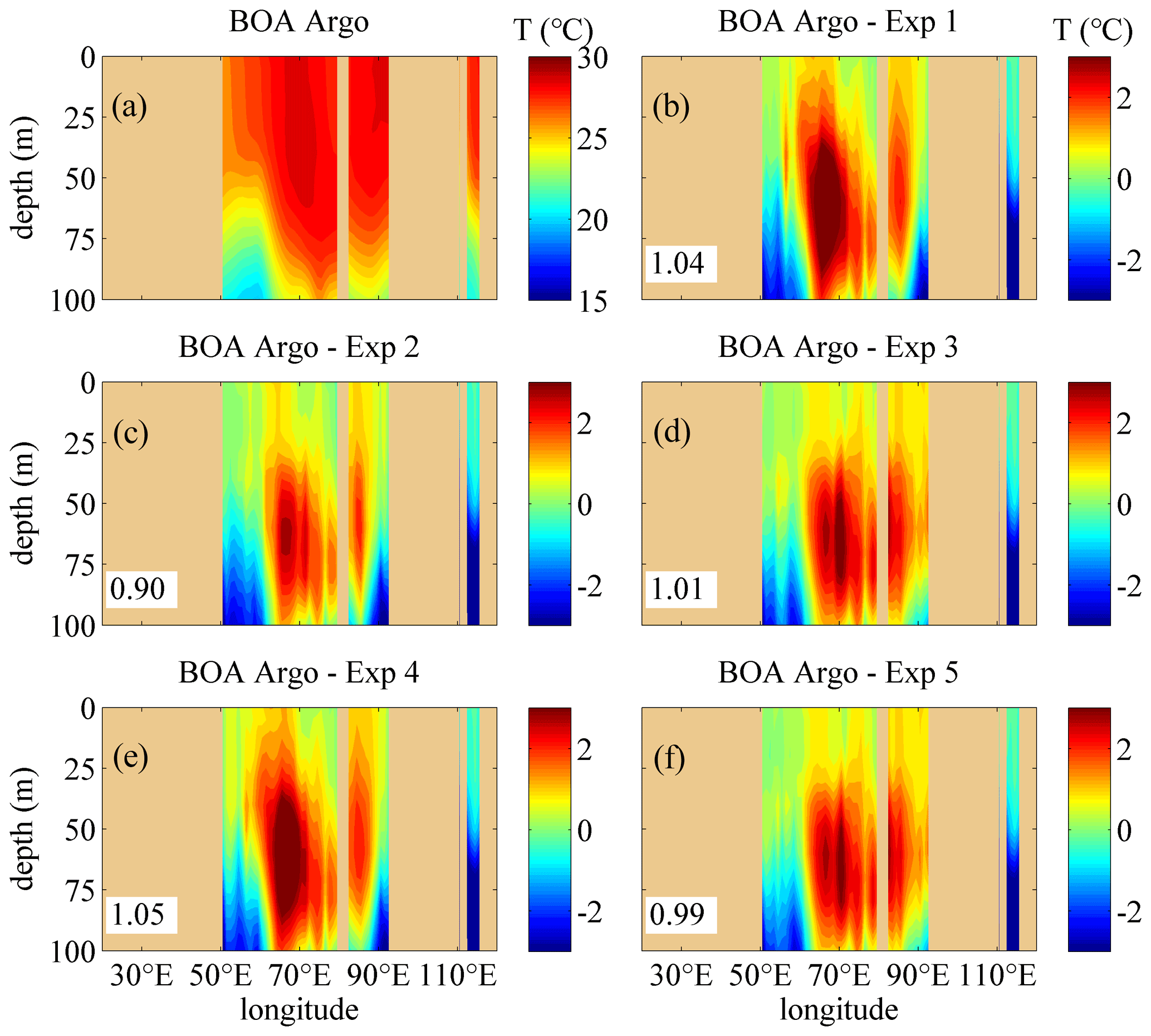
In order to evaluate the modeling results further, the existing Argo-derived gridded products, which are named Barnes objective analysis-Argo (BOA-Argo) datasets (Li et al., 2017), are also chosen. The climatologic monthly mean BOA-Argo data (multiyear mean from 2004 to 2014) are used and can be downloaded directly from ftp://data.argo.org.cn/pub/ARGO/BOA_Argo/ (last access: 5 September 2022). The BOA-Argo data with 49 vertical levels from the surface to 1950 m depth are produced based on refined Barnes successive corrections by adopting flexible response functions. A series of error analyses is adopted to minimize errors induced by the nonuniform spatial distribution of Argo observations. These response functions allow BOA-Argo to capture a greater portion of mesoscale and large-scale signals while compressing small-sale and high-frequency noise. The performance of the BOA-Argo dataset demonstrates both accuracy and retainment of mesoscale features. Generally, BOA-Argo seems to compare well with other global gridded datasets (Li et al., 2017).

Figures 10 and 11 show the comparison of the temperature structure between the monthly BOA-Argo data and the model results in January. The vertical distributions are similar to those from the WOA13 data (see panel a in Figs. 4, 6, 10 and 11). The difference between the BOA-Argo data and the model results along 30.5^∘ S is also similar to the WOA13 data. Compared with Exp 1, the difference for Exp 2 often decreases remarkably, and the difference for Exp 3 is much smaller than that of Exp 1 and Exp 2 because of the incorporation of the IT-generated turbulent mixing, especially in the layers with depths between 20 and 50 m. In addition, the improvement of the NBSW and IT along 7.5^∘ N is not obvious; this conclusion is also similar to that for the WOA13 data. This implies that the three mixing schemes introduced in this study may not be appropriate in the marginal sea simulation that is full of small-scale and mesoscale processes. In order to solve the issues about the accuracy, we attempt to design high-resolution real-time numerical modeling experiments in the NIO (or the Arabian Sea and the Bay of Bengal only), as well as finer simulation of surface waves and more accurate estimation of ITs.

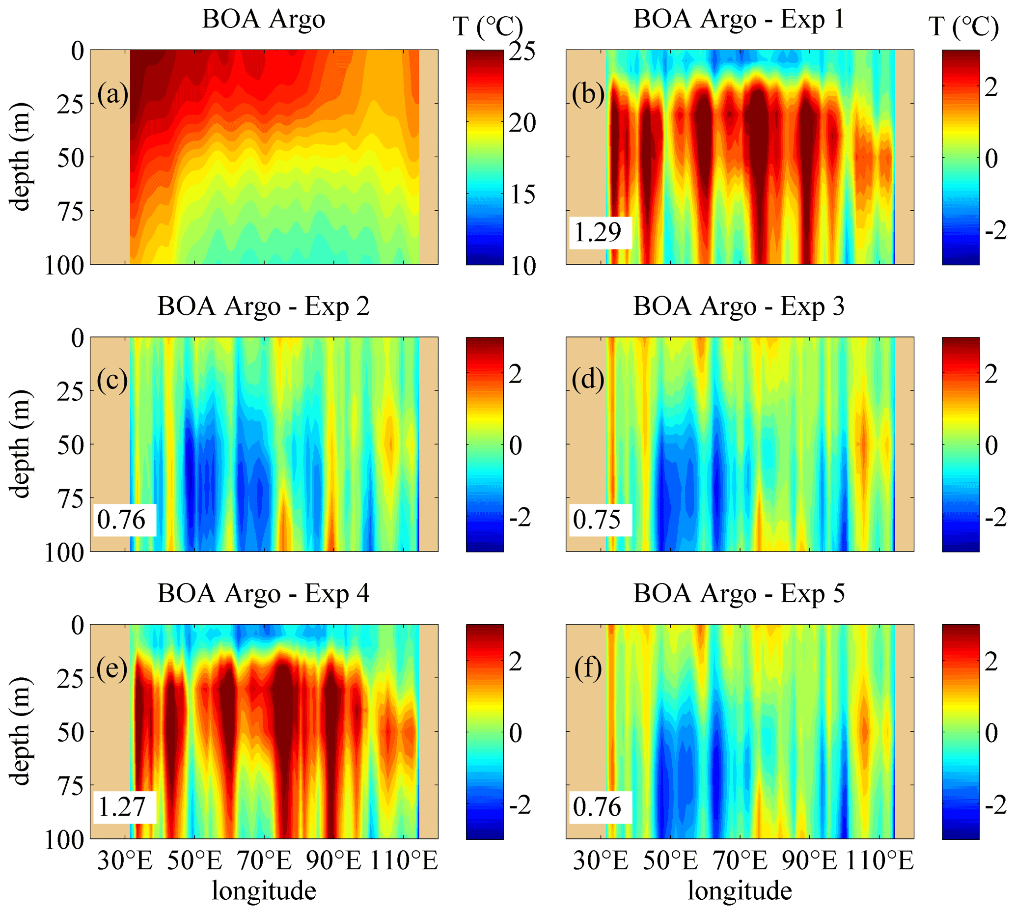
Figure 10 The vertical temperature profiles along 30.5^∘ S in January. (a) The temperature structure from the monthly BOA-Argo data (units: degrees). (b–f) The difference of the temperature calculated by subtracting the monthly mean results simulated in Exp 1–Exp 5 from the monthly BOA-Argo data, respectively. The RMSEs of the temperature in the upper 100 m regions between the BOA-Argo data and the model results are given. Deep yellow areas correspond to land.

Figure 11 The same as Fig. 10, but along 7.5^∘ N.

4.3 Effects on simulation of the mixed layer depth

The mixed layer (ML), which is characterized by quasi-uniform temperature and salinity, is crucial in understanding the physical processes in the upper ocean. The MLD variability is influenced by many processes including wind-induced turbulence, surface warming or cooling, air–sea heat exchange and turbulence–wave interaction (Chen et al., 1994; Kara et al., 2003; de Boyer Montégut et al., 2004; Abdulla et al., 2019). There are different methods to define the MLD (Kara et al., 2003). The threshold criterion, which is a widely favored and simple method for finding the MLD (Kara et al., 2003; de Boyer Montégut et al., 2004), is used in this study. In the threshold criterion, the MLD is defined as the depth at which the temperature or density profiles change by a predefined amount relative to a surface reference value. Various temperature threshold criteria were used to determine the MLD globally, such as 0.2^∘ in de Boyer Montégut et al. (2004), 0.5^∘ in Monterey and Levitus (1997), 0.8^∘ in Kara et al. (2003) and 1.0^∘ in Qiao et al. (2010). Therefore, considering the vertical temperature distribution pattern in the IO, we choose one of the typical threshold criteria (1.0^∘) to define the MLD and attempt to make the effects of NBSWs and ITs on the simulated MLD more obvious. In this study, the MLD is defined as the depth at which the temperature is lower than the SST by 1.0^∘ and is used to show the upper-ocean thermal structure.

Figure 12 shows the comparisons of the MLDs between the WOA13 data and the model results in January. The MLDs for Exp 1 are generally shallower than WOA13 in the whole IO and the Southern Ocean because of insufficient simulated mixing processes, which leads to underestimation of the vertical mixing in the upper ocean, especially during summer. The conclusion is similar to the global and regional simulations in previous studies (Kantha and Clayson, 1994; Qiao et al., 2010; Wang et al., 2019; Zhuang et al., 2020). The accumulation of weak vertical mixing during the 10-year climatologic modeling will make more heat staying in the surface layer, which will lead to warmer SST and shallower MLDs. In fact, from Fig. 12 one can see that the obviously shallower MLDs are generally in the ACC regions where the simulated vertical mixing from the original experiment is dramatically weak. In addition to the ACC regions, the obviously shallower MLDs also appear in the east regions of the Arabian Sea because of the weak vertical mixing. Furthermore, the simulated MLDs in most of the tropical and southern regions of the IO are partially shallower than the WOA13 data. Adopting the threshold criterion of 1.0^∘, the simulated MLDs were shallower than the WOA13 data because of the warmer SST and cooler temperature in the ocean interior. Comparisons among the MLDs for Exp 1–Exp 3 show that the NBSW and IT may enhance upper-ocean mixing and make the simulated MLDs closer to the WOA13 data. The MLs for Exp 2 and Exp 3 are extremely deepened, especially in the tropical IO and the Southern Ocean. The RMSEs of the MLDs between the WOA13 data and the model results decrease 13.2 % and 14.6 % from 21.9 m (Exp 1) to 19.0 m (Exp 2) and to 18.7 m (Exp 3), respectively. However, the effects of the WTFR seem to be trivial in the whole area because there is almost no improvement from Exp 4–5 to Exp 1 and 3. The RMSEs for Exp 4–5 are larger than for Exp 1 and 3, and the larger deviations in Exp 4–5 mostly occur in the Southern Ocean, implying that the WTFR does not work well in the Southern Ocean in austral winter.

Figure 12 The distribution of the MLD calculated from WOA13 data and the differences of the MLD between the WOA13 data and the results simulated in Exp 1–Exp 5. RMSEs of the MLD are shown in the upper left corner of the panels. Deep yellow and white areas correspond to land, and the calculated MLDs are deeper than 150 m.

4.4 Effects on simulation of ocean currents

In this subsection, the simulated horizontal velocities in the surface layer are analyzed to evaluate the effects of NBSWs and ITs on ocean currents. Previous studies indicated that NBSWs and ITs have complicated impacts on simulated currents for OGCMs (e.g., Huang and Qiao, 2010; Wu et al., 2019). Only the results simulated in Exp 1–Exp 3 are discussed in detail, and the results in Exp 4 and Exp 5 are omitted here because the effects of the WTFR-induced mixing are relatively small. This situation is similar to the simulated temperature structure and MLDs in Sect. 4.2 and 4.3.

Figure 13 shows the comparisons of the surface velocities between the monthly mean OSCAR data (Bonjean and Lagerloef, 2002) and the model results of Exp 1–Exp 3 in January and July. The simulated surface velocities are chosen as those at the depth of 2 m interpolated by the model results. The OSCAR surface current products with a horizontal resolution of 1^∘ $/$ 3 × 1^∘ $/$ 3 and a time resolution of 5 d are constructed from the altimeter SSH, scatterometer winds, and both radiometer and in situ SST. The velocities are calculated based on a combined formulation including geostrophic balance, Ekman–Stommel dynamics and a complementary term for SST gradients (Bonjean and Lagerloef, 2002; Dohan, 2017). Johnson et al. (2007) demonstrated that OSCAR products are able to provide accurate estimates of the surface time mean circulation. A 29-year (1993–2021) time series of the OSCAR surface current data is collected and used to calculate the monthly mean climatologic currents, which are regarded as the reference in the comparison. In Fig. 13a and b, the spatial distribution of the surface current fields is presented as the anticyclonic subtropical gyre in the SIO and the monsoonally forced circulation of the tropics and the NIO (clockwise in boreal summer and anticlockwise in boreal winter). The eastern boundary current (Leeuwin Current) is not obvious because of the too small magnitude of the velocities in the climatologic data. Figure 13c–h present the difference by subtracting the monthly OSCAR data from the mean results of the three experiments. Generally, the simulated results contain most features of the surface currents in the IO. However, the simulated velocities are relatively too large to the southwest of the Indian Peninsula in January and too small in the Somali Current and the ACC regions in both January and July. The reason should be that the spatial and temporal resolution as well as the accuracy of the surface forcing data are insufficient. One can see that there is only a little difference in the simulated currents among the three experiments. The relatively smallest RMSEs for Exp 3 indicate that the NBSW and IT are able to improve the simulated surface currents.

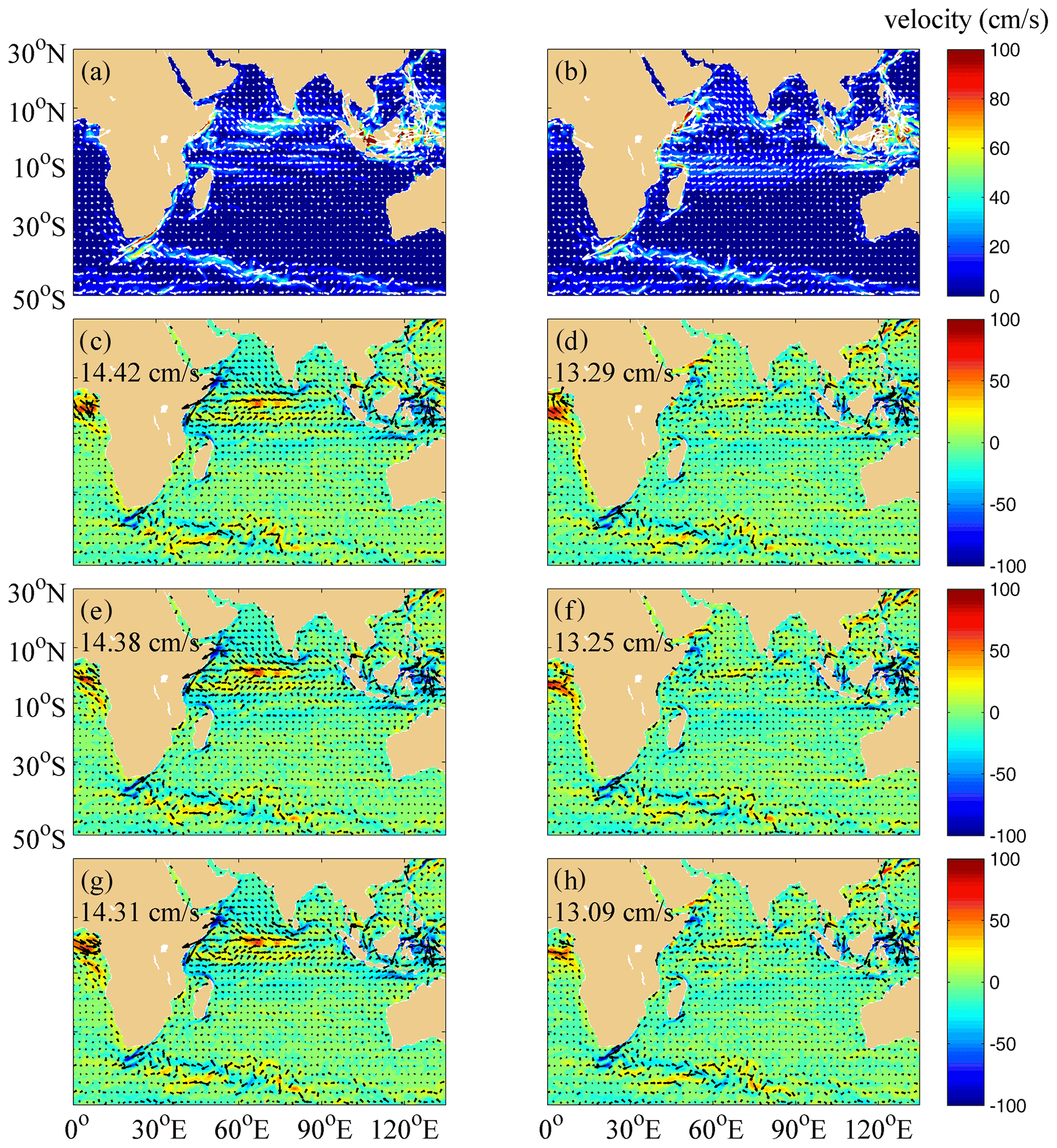
Figure 13 The distribution of surface currents from the OSCAR climatologic data and the differences by subtracting the OSCAR data from the mean results from Exp 1 (c, d), Exp 2 (e, f) and Exp 3 (g, h) in January (c, e, g) and July (d, f, h). RMSEs of the surface velocities are shown in the upper left corner of the panels. White arrows in panels (a) and (b) represent the surface current vectors, and black arrows in panels (c)–(h) represent the surface current difference vectors. Deep yellow areas correspond to land.

Furthermore, we calculated the three-dimensional vertical vorticity and eddy kinetic energy (EKE) in Exp 1–Exp 5 to evaluate the effects of mixing induced by NBSWs and ITs on the mesoscale eddy activity. However, the difference of the vertical vorticity and the EKE among the five experiments was too complicated to summarize some dynamic processes and physical mechanisms. The reason should be that the climatological modeling in this study, on one hand, may be inappropriate to analyze mesoscale or small-scale processes because of the relatively coarse resolution, smoothed surface forcing, open boundary conditions and topography data; on the other hand, the induced vertical mixing may not be a key mechanism for eddy activity, as previous studies indicated that surface waves affect eddies through the interaction among the turbulence, circulation and Langmuir circulation when the turbulent Langmuir number is small (Jayne and Marotzke, 2002; Romero et al., 2021); subharmonic instability may transfer the energy from the internal tides to the shear-induced turbulent diapycnal mixing (MacKinnon and Gregg, 2005; Pinkel and Sun, 2013). Especially in the east region of the tropical Indian Ocean, the effects of the ITF on mesoscale or small-scale processes have not yet been simulated exactly in existing OGCMs (e.g., Nagai et al., 2017; Santoso et al., 022). Additional improvements of the mixing schemes and the ocean modeling will be studied further in the future.

5 Discussion

We evaluate the impacts of three different mixing schemes, including NBSW-generated turbulent mixing, WTFR-induced mixing and IT-generated turbulent mixing, on the upper-ocean thermal structure simulation in the IO. The comparisons of the temperature structure and the MLDs between the WOA13 data, which are regarded as the observations, and the model results imply that the simulation is significantly improved by incorporating the NBSW- and IT-generated turbulent mixing into the MASNUM ocean circulation model, but the effects of the WTFR are trivial, and the simulated MLDs are even deteriorated in some regions. However, based on numerical experiments, Yang et al. (2019) demonstrated that the WTFR may play an important role in SST cooling if the wind and surface waves are strong. During the period of tropical cyclone Nepartak passage, the simulated SST cooling distribution and the cooling amplitude are more consistent with the observations if the WTFR-induced mixing scheme is incorporated, which presents warming and cooling effects on the left and right sides of the typhoon track (Yu et al., 2020). The effects of the WTFR under the typhoon conditions will be further examined in future work.

In addition, the three mixing schemes are incorporated into the MASNUM model as part of the vertical diffusive terms, thus avoiding issues that may result from adding the mixing coefficients to those from the M-Y 2.5 scheme directly. The analysis of the numerical results indicates that the NBSW (and WTFR sometimes) leads to improved simulations of upper-ocean temperature structure and MLDs due to the enhanced mixing that draws warmer water from the surface to the subsurface layers with depths from about 10 to 40 m. Then the IT, which can improve the simulations further, may enhance the mixing that draws warmer water from the subsurface layers to the ocean interior (Fig. 14). In summary, the combination of NBSW- and IT-generated turbulent mixing results in a better match with observations of upper-ocean temperature structure and MLDs. The mixing schemes introduced in this study contain the effects of surface waves and internal tides, which are thought to supplement the physical mechanism for the vertical mixing processes in OGCMs because the original turbulent mixing schemes, such as the M-Y 2.5 scheme, neglected the interaction between surface waves and currents (Huang and Qiao, 2010; Huang et al., 2011). The M-Y 2.5 mixing scheme combined with the NBSW- and IT-induced mixing schemes should become more complete for modeling vertical mixing processes. In our opinion, it is important to study NBSW- and IT-induced mixing for promoting the development of the ocean and coupling models.

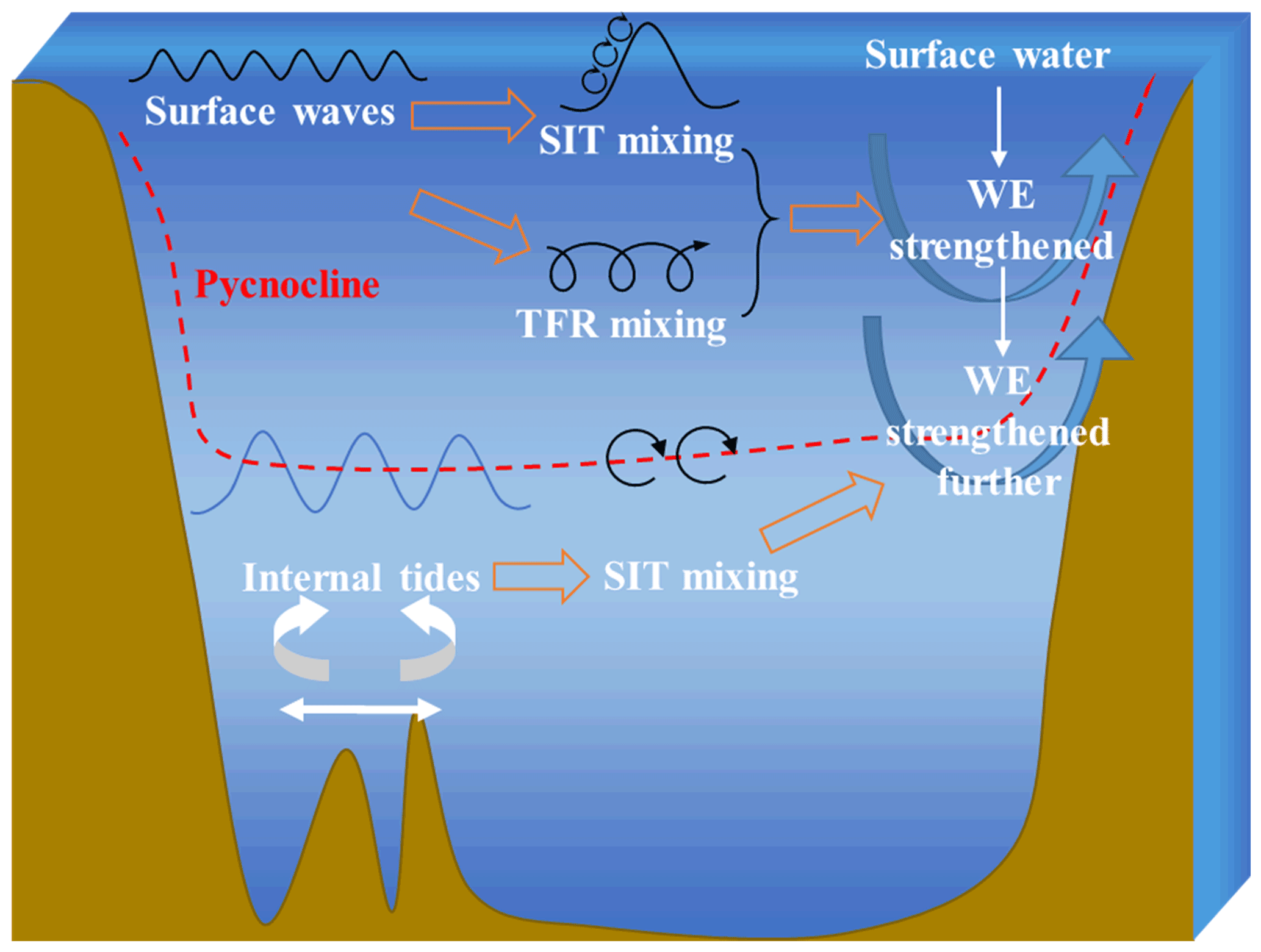
Figure 14 Sketch of the enhancing processes of the vertical mixing induced by three different mechanisms, including NBSW-generated turbulent mixing, WTFR-induced mixing and IT-generated turbulent mixing. SIT and TFR mixing represent the shear-induced turbulent and transport flux residue mixing, respectively. WE means the water exchange.

It is worth noting that the circulation and temperature structure of the IO have not yet been characterized by the ocean model in the present study because of the non-ignorable difference between the WOA13 data and the simulation results. The RMSEs in the NIO, including the Arabian Sea and the Bay of Bengal, are even generally larger than 1.2^∘. Direct modeling of ITs in the experiments of this study is inappropriate. Firstly, the horizontal and vertical resolution could be insufficient to simulate the generation and propagation of ITs because of the relatively coarse topography and coastlines. The modeling area of the whole IO could also be too large. Secondly, the MASNUM ocean model used in this study does not yet include the tidal forcing and tidal open boundary conditions, so the conversion from barotropic to baroclinic energy cannot be described exactly. Finally, the climatologic experiments are not good at simulating ITs because the multiyear mean surface forcing could be very smooth and partly lack the local small-scale and mesoscale information. The climatologic current, temperature and salinity input in the open boundary is also inappropriate for IT modeling. Therefore, higher horizontal resolution and more vertical layers, on one hand, will be designed in following experiments to describe the finer structure and features of the IO. On the other hand, the surface forcing and lateral boundary conditions with higher spatial and temporal resolution, such as the ERA5 hourly reanalysis data (https://cds.climate.copernicus.eu/cdsapp#!/dataset/reanalysis-era5-single-levels?tab=form, last access: 1 September 2022), the Climate Forecast System Version 2 (CFSv2) (http://rda.ucar.edu/datasets/ds094.0/, last access: 20 April 2022) and the global HYbrid Coordinate Ocean Model/Navy Coupled Ocean Data Assimilation (HYCOM/NCODA) product (https://www.hycom.org/data/glba0pt08/expt-90pt8, last access: 15 September 2022), as well as more optimization and improvement of the real-time hindcast experimental design will be used to simulate the IO more accurately. It is worth noting that the NBSW and IT can obviously improve the simulation in the Arabian Sea but do not always work in the Bay of Bengal, which is a hot spot for the generation of ITs. This implies that the IT-induced mixing scheme may not be appropriate in the marginal sea simulation containing small- and mesoscale processes.

We have to admit that the issues about the simulation in the IO cannot be solved entirely when the NBSW- and IT-induced mixing schemes are adopted, but it should be more convenient to improve the ocean modeling further because the mixing schemes are independent of the ocean models. A multi-scale process coupling model, including the atmosphere, ocean currents, tides, surface waves, and internal wave and tide component models, will be established in the future for accurate and high-resolution ocean and atmosphere modeling. The NBSW- and IT-induced mixing schemes and the related results in this study are helpful and valuable for establishing the coupling model.

6 Conclusions

This study uses the MASNUM ocean circulation model for testing and validating the effects of three different mixing schemes, including NBSW-generated turbulent mixing, WTFR-induced mixing and IT-generated turbulent mixing, on the upper-ocean thermal structure simulation in the IO. The major findings are summarized as follows.

1. The diffusive terms calculated by NBSW-generated turbulent mixing are dominant if the depth is less than 30 m, while WTFR-induced mixing is extremely weak because the values are about 4 to 6 orders smaller than the NBSW. In the ocean interior with depths from 40 to 130 m, the diffusive terms calculated by the IT-generated turbulent mixing are the largest ones in regions with large topographic relief.

2. The effects of these schemes on the upper-ocean simulation are tested. The results show that the simulated thermal structure, MLDs and surface currents are improved by the NBSW because of the enhanced mixing in the sea surface, while the effects of the WTFR are trivial.

3. The IT may strengthen the vertical mixing of the ocean interior and improve the simulation further. In summary, the combination of the NBSW and IT may strengthen vertical mixing and improve the upper-ocean simulation.

Appendix A: The velocity shear module of the internal tide

Internal-tide-induced mixing plays an important role in the vertical and horizontal distribution of water mass properties. Based on the Navier–Stokes equations, the solvability simplification is realized based on the spatiotemporal scale, controlling mechanism and actual characteristics of the ITs. The IT is considered to be weakly nonlinear, the shear terms of the larger-scale motions in the equations are approximately linear, and the molecular and turbulent mixing terms in the equations are too small to be ignored. The f plane and layered approximation for the larger-scale motions are also adopted into the equations. Thus, the simplified equations can be written as

$$\begin{array}{}\text{(A1)}& {\displaystyle \frac{\partial u_{\mathrm{IT}\mathrm{1}}}{\partial x_{\mathrm{1}}}}+{\displaystyle \frac{\partial u_{\mathrm{IT}\mathrm{2}}}{\partial x_{\mathrm{2}}}}+{\displaystyle \frac{\partial u_{\mathrm{IT}\mathrm{3}}}{\partial x_{\mathrm{3}}}}+\mathit{\gamma }{u}_{\mathrm{IT}\mathrm{1}}=\mathrm{0},\text{(A2)}& {\displaystyle \frac{\partial u_{\mathrm{IT}\mathrm{1}}}{\partial t}}-f{u}_{\mathrm{IT}\mathrm{2}}-\mathrm{2}{U}_{\mathrm{1}}\mathit{\gamma }{u}_{\mathrm{IT}\mathrm{2}}=-{\displaystyle \frac{\partial }{\partial x_{\mathrm{1}}}}\left({\displaystyle \frac{p_{\mathrm{IT}}}{{\mathit{\rho }}_{\mathrm{0}}}}\right),\text{(A3)}& {\displaystyle }\begin{array}{rl}{\displaystyle \frac{\partial u_{\mathrm{IT}\mathrm{2}}}{\partial t}}& +\left(f+\mathrm{2}\mathit{\gamma }{U}_{\mathrm{2}}+{\displaystyle \frac{\partial U_{\mathrm{2}}}{\partial x_{\mathrm{1}}}}\right)u_{\mathrm{IT}\mathrm{1}}+{\displaystyle \frac{\partial U_{\mathrm{2}}}{\partial x_{\mathrm{3}}}}{u}_{\mathrm{IT}\mathrm{3}}\\ & =-{\displaystyle \frac{\partial }{\partial x_{\mathrm{2}}}}\left({\displaystyle \frac{p_{\mathrm{IT}}}{{\mathit{\rho }}_{\mathrm{0}}}}\right),\end{array}\text{(A4)}& {\displaystyle \frac{\partial u_{\mathrm{IT}\mathrm{3}}}{\partial t}}=-{\displaystyle \frac{\partial }{\partial x_{\mathrm{3}}}}\left({\displaystyle \frac{p_{\mathrm{IT}}}{{\mathit{\rho }}_{\mathrm{0}}}}\right)-g\left({\displaystyle \frac{{\mathit{\rho }}_{\mathrm{IT}}}{{\mathit{\rho }}_{\mathrm{0}}}}\right),\text{(A5)}& {\displaystyle \frac{\partial }{\partial t}}\left({\displaystyle \frac{{\mathit{\rho }}_{IT}}{{\mathit{\rho }}_{\mathrm{0}}}}\right)+{\displaystyle \frac{\partial }{\partial x_{\mathrm{1}}}}\left({\displaystyle \frac{{\mathit{\rho }}_{\mathrm{IT}}}{{\mathit{\rho }}_{\mathrm{0}}}}\right)u_{\mathrm{IT}\mathrm{1}}+{\displaystyle \frac{\partial }{\partial x_{\mathrm{3}}}}\left({\displaystyle \frac{{\mathit{\rho }}_{\mathrm{IT}}}{{\mathit{\rho }}_{\mathrm{0}}}}\right)u_{\mathrm{IT}\mathrm{3}}=\mathrm{0},\end{array}$$

where u_ITi (i=1, 2, 3), ρ_IT and p_IT denote the three-dimensional velocity, density and pressure of the internal tide, respectively. f is the Coriolis parameter, and γ is regarded as the curvature of the larger-scale motions including mesoscale eddies, gyres and so on. U_i represents the velocity of the larger-scale motions. The Fourier kernel function is used to transform the differential equations in Eqs. (A1) to (A5) to the algebraic equations; for example, the relation between $u_{{\mathrm{IT}}_{\mathrm{1}}}$ and its Fourier kernel function μ_IT1 can be expressed as

$$\begin{array}{}\text{(A6)}& u_{\mathrm{IT}\mathrm{1}}=\int \underset{\mathit{k}}{\int }{\mathit{\eta }}_{\mathrm{IT}}{\mathit{\mu }}_{\mathrm{IT}\mathrm{1}}\exp \left\{i\left(k_{\mathrm{1}}{x}_{\mathrm{1}}+k_{\mathrm{2}}{x}_{\mathrm{2}}-\mathit{\omega }t\right)\right\}\mathrm{d}{k}_{\mathrm{1}}\mathrm{d}{k}_{\mathrm{2}},\end{array}$$

where η_IT is the SSH amplitude of the internal tide, and ω is the frequency. The dispersion relation between the frequency and the wavenumber can be written as

$$\begin{array}{}\text{(A7)}& {\displaystyle }\begin{array}{rl}{\mathit{\omega }}^{\mathrm{2}}{\left({\displaystyle \frac{N_{\mathrm{0}}^{\mathrm{2}}}{{\mathit{\omega }}^{\mathrm{2}}}}-\mathrm{1}\right)}^{\frac{\mathrm{1}}{\mathrm{2}}}& =g\left({\displaystyle \frac{{\mathit{\rho }}_{\mathrm{IT}}}{{\mathit{\rho }}_{\mathrm{0}}}}\right)\\ & \cdot k{\displaystyle \frac{\sin \left\{{\int }_{-H}^{\mathrm{0}}{\left(\frac{N^{\mathrm{2}}}{{\mathit{\omega }}^{\mathrm{2}}}-\mathrm{1}\right)}^{\frac{\mathrm{1}}{\mathrm{2}}}k\mathrm{d}{x}_{\mathrm{3}}\right\}}{\cos \left\{{\int }_{-H}^{\mathrm{0}}{\left(\frac{N^{\mathrm{2}}}{{\mathit{\omega }}^{\mathrm{2}}}-\mathrm{1}\right)}^{\frac{\mathrm{1}}{\mathrm{2}}}k\mathrm{d}{x}_{\mathrm{3}}\right\}}},\end{array}\text{(A8)}& {\displaystyle \frac{\partial \mathit{\omega }}{\partial x_{\mathrm{3}}}}=\mathrm{0}.\end{array}$$

Based on the analytical expression of the three-dimensional velocity (derived from the Fourier kernel functions) and Eqs. (A7) and (A8), the velocity shear module can be expressed analytically as

$$\begin{array}{}\text{(A9)}& \begin{array}{rl}& {\left(\sum _{i=\mathrm{1}}^{\mathrm{3}}\sum _{j=\mathrm{1}}^{\mathrm{3}}\left|{\displaystyle \frac{\partial u_{\mathrm{IT}i}}{\partial x_j}}\right|\right)}^{\mathrm{2}}\\ & ={\left\{\mathrm{2}\int \underset{\mathit{k}}{\int }{\mathit{\eta }}_{\mathrm{IW}}{k}^{\mathrm{2}}{\mathit{\omega }}^{\mathrm{2}}{\displaystyle \frac{{\left(\frac{N^{\mathrm{2}}}{\mathrm{2}{\mathit{\omega }}^{\mathrm{2}}}\right)}^{\mathrm{2}}-{\left(\frac{N^{\mathrm{2}}}{\mathrm{2}{\mathit{\omega }}^{\mathrm{2}}}-\mathrm{1}\right)}^{\mathrm{2}}\cos \left\{\mathrm{2}{\int }_{-H}^{x_{\mathrm{3}}}{\left(\frac{N^{\mathrm{2}}}{{\mathit{\omega }}^{\mathrm{2}}}-\mathrm{1}\right)}^{\frac{\mathrm{1}}{\mathrm{2}}}k\mathrm{d}{x}_{\mathrm{3}}\right\}}{{\sin }^{\mathrm{2}}\left\{{\int }_{-H}^{\mathrm{0}}{\left(\frac{N^{\mathrm{2}}}{{\mathit{\omega }}^{\mathrm{2}}}-\mathrm{1}\right)}^{\frac{\mathrm{1}}{\mathrm{2}}}k\mathrm{d}{x}_{\mathrm{3}}\right\}}}\mathrm{d}{k}_{\mathrm{1}}\mathrm{d}{k}_{\mathrm{2}}\right\}}^{\frac{\mathrm{1}}{\mathrm{2}}},\end{array}\end{array}$$

which is consistent with Eq. (5). Similar to Gregg (1989) and Gregg and Kunze (1991), the mixing terms including the viscosity and diffusivity can be calculated from the velocity shear modules as shown in Eq. (4).