the Creative Commons Attribution 4.0 License.
the Creative Commons Attribution 4.0 License.
 | 16 Sep 2022
Introduction of the DISAMAR radiative transfer model: determining instrument specifications and analysing methods for atmospheric retrieval (version 4.1.5)
Johan F. de Haan
Ping Wang
Maarten Sneep
J. Pepijn Veefkind
Piet Stammes
DISAMAR (determining instrument specifications and analysing methods for atmospheric retrieval) is a computer model developed to simulate retrievals of properties of atmospheric trace gases, aerosols, clouds, and the ground surface from passive remote sensing observations in a wavelength range from 270 to 2400 nm. It is being used for the TROPOMI/Sentinel-5P and Sentinel-4/5 missions to derive Level-1b product specifications. DISAMAR uses the doubling–adding method and the layer-based orders of scattering method for radiative transfer calculations. It can perform retrievals using three different approaches: optimal estimation (OE), differential optical absorption spectroscopy (DOAS), and the combination of DOAS and OE, called DISMAS (differential and smooth absorption separated). The derivatives, which are needed in the OE and DISMAS retrievals, are derived in a semi-analytical way from the adding formulae. DISAMAR uses plane-parallel homogeneous atmospheric layers with a pseudo-spherical correction for large solar zenith angles. DISAMAR has various novel features and diverse retrieval possibilities, such as retrieving aerosol layer heights and ozone vertical profiles. This paper provides an overview of the DISAMAR model version 4.1.5 without treating all the details. We focus on the principle of the layer-based orders of scattering method, the calculation of the semi-analytical derivatives, and the DISMAS retrieval method, and it is to our knowledge the first time that these methods are described. We demonstrate some applications of DISMAS and the derivatives.
- Article
(2083 KB) - Full-text XML
- BibTeX
- EndNote


DISAMAR stands for determining instrument specifications and analysing methods for atmospheric retrieval. It is a computer code written in Fortran 90 to simulate retrievals of atmospheric components like trace gases, aerosols, and clouds and properties of the ground surface from passive remote sensing observations of the Earth. The wavelength range considered is from 270 to 2400 nm. The development of DISAMAR started around the year 2000 but made use of the heritage of doubling–adding code from the 1980s (De Haan et al., 1987). Initially, DISAMAR was developed to derive Level-1b radiance requirements given specific Level-2 geophysical product requirements for satellite instruments. In order to derive Level-1b requirements for a given requirement for a Level-2 product, the model has to simulate instrument features and perform retrievals for the Level-2 product with proper error estimation. From the European satellite missions Sentinel-5P (with TROPOMI on board Veefkind et al., 2012), Sentinel-4, and Sentinel-5, atmospheric trace gases, cloud, and aerosol products have to be generated from the measured radiance spectra. In principle, it is possible to simulate Level-1b spectra using a radiative transfer (RT) model to modify the simulated spectra with instrument features, like noise, and then run a retrieval algorithm. However, this can introduce inconsistencies between the RT model simulation and the retrieval algorithm, which makes the error estimate of the Level-2 product less accurate. With DISAMAR providing the end-to-end calculation for all the steps from instrument response to retrieved geophysical product, a high degree of internal consistency is achieved. For example, DISAMAR has been used to calculate Level-1b requirements for preparation of the Sentinel-4, Sentinel-5, Sentinel-5P and other missions (e.g. De Haan, 2009, 2010, 2012; Sanders et al., 2015; Nanda et al., 2018).
DISAMAR contains a radiative transfer module to simulate radiance, irradiance, and sun-normalized radiance (or reflectance). The radiative transfer is based on the doubling–adding method and includes a more efficient variant, called layer-based orders of scattering (LABOS). Polarization (Stokes four-vectors and 4×4 Mueller matrices) and rotational Raman scattering (RRS) are included in DISAMAR. The implementation of RRS is based on the publications by Chance and Spurr (1997) and Stam et al. (2002). The derivatives of the radiance or reflectance with respect to the retrieved parameters (also called weighting functions or Jacobians) that are needed for the retrievals are calculated using efficient semi-analytical expressions. The atmosphere is assumed to be plane-parallel with an option for pseudo-spherical correction. Three types of retrievals are available, namely optimal estimation (OE) (Rodgers, 2000), DOAS (differential optical absorption spectroscopy) (Platt, 1994), and DISMAS (differential and smooth absorption separated), a version of OE based on a DOAS-like approach. The choice of DOAS and OE retrievals is driven by the Level-2 retrieval algorithms for atmospheric trace gas columns (using DOAS) and ozone profiles (using OE).
A cloud or aerosol layer can be modelled by a simple reflecting Lambertian surface or by a layer of scattering particles with a Henyey–Greenstein phase function or a phase function using expansion coefficients that are read from file (e.g. Mie scattering particles). The surface below the atmosphere is a Lambertian reflector with an albedo that can vary with wavelength. In addition, surface emissions can be included to simulate sun-induced fluorescence (Frankenberg et al., 2011).
The applications of DISAMAR are retrievals of the ozone profile from the ultra-violet (UV), the total column of NO2 from the visible (VIS), cloud properties (height, fraction, optical thickness) from the O2 A-band in the near-infrared (NIR), or CO2 from the shortwave infrared (SWIR). The simulated measurements can be modified by adding noise, offsets to the wavelength scales, and offsets to the radiance and solar irradiance. By evaluating the effects of these modifications on retrieved parameters, requirements on the Level-1b measured spectra can be derived. By changing the a priori error of auxiliary data (e.g. surface albedo) the required accuracy of auxiliary data can be determined.
Due to the time-consuming line-by-line calculations, DISAMAR is not suitable for fast computation or applications in numerical weather prediction (NWP) models. We would recommend RTTOV (Saunders et al., 2018) and CRTM (e.g. Lu et al., 2021; Karpowicz et al., 2022; Stegmann et al., 2022) as fast radiative transfer models for NWP applications. DISAMAR has actually been used to benchmark RTTOV in the UV–visible wavelength range.
The advantage of DISAMAR is that it includes diverse instrument features, simulations, and retrieval algorithms in one code. For such a complex model, it is not possible to cover all details in one paper. We therefore highlight the novel and unique features of DISAMAR (version 4.1.5), which are listed in Sect. 2. Section 3 presents the forward simulations. The retrieval part is described in Sect. 4. Some applications are shown in Sect. 5 as examples. Section 6 presents a discussion and conclusions.
DISAMAR uses a separate altitude grid for the radiative transfer calculations, which is independent of the grid used for specifying the atmospheric properties. This makes it possible to deal with strong vertical gradients in the radiation field, e.g. near the top of clouds.
The altitude grid, wavelength grid, and polar angles are all defined using Gauss–Legendre division points. This makes the integration over altitude, wavelength, or polar angle more accurate than the integration with an equidistant grid using a similar number of grid points.
The number of streams used for integration over polar angles when multiple scattering is involved can be arbitrarily large. The number of coefficients used for the expansion of the phase function in Legendre functions can also be arbitrarily large. All of these features make the DISAMAR calculations more accurate.
DISAMAR provides not just the radiance spectrum of the backscattered sunlight but also the derivatives with respect to the elements of the state vector. These derivatives are essential in OE and are used to find the solution in an iterative manner. They are also used to determine the error covariance matrix, gain vectors, and the averaging kernel (Rodgers, 2000). In DISAMAR all derivatives are calculated in a semi-analytical manner, although algorithmic differentiation can be used to evaluate the derivatives (Griewank and Walther, 2008). The calculation of the derivatives in DISAMAR takes no more than 10 %–30 % of the total calculation time.
Because DISAMAR was originally developed to determine instrument specifications and analyse methods for atmospheric retrieval, special emphasis is given to the error information of the retrieved products and instrumental features. The main retrieval algorithm is optimal estimation (OE) (Rodgers, 2000). Therefore, DISAMAR provides full diagnostic information, including error covariance matrices and averaging kernels. It can deal with combined retrievals using information from different wavelength bands. OE is used for ozone profile retrieval by DISAMAR. The retrieved ozone profiles consist of the volume mixing ratio (VMR) of ozone at each altitude, obtained through spline interpolation or linear interpolation on the logarithm of the VMR given at a user-defined altitude grid. This makes conversion from VMR to Dobson units per layer and from VMR to number densities simple.
By using the newly developed DISMAS approach, which combines the principle of the DOAS retrieval method with OE, the number of wavelengths at which forward calculations have to be performed can be reduced significantly.
The forward model of DISAMAR provides simulated radiance (or sun-normalized radiance) and irradiance and the derivatives of the radiance with respect to the state vector elements. The semi-analytical approach computes the forward-mode (tangent-linear) derivatives of the radiance spectrum. Here, attention is given to the calculation of these derivatives using a semi-analytical approach because this important aspect for retrievals has not been published before.
3.1 Instrument model
The simulated radiance and irradiance can be convoluted separately with the instrument spectral response function (ISRF). The ISRF is defined in terms of a convolution operator. A Gaussian ISRF and a flat-topped ISRF are included in DISAMAR. A tabulated ISRF, e.g. measured for a specific instrument, can also be used as an external file. During the convolution, the wavelength grid of the ISRF is interpolated to a high-resolution wavelength grid (see Sect. 3.2.1 for the high-resolution wavelength grid). The instrument features, such as signal-to-noise ratio (SNR), stray light, and wavelength calibration errors, can be simulated using DISAMAR by specifying corresponding entries in a configuration file.
3.2 Atmospheric and surface properties
3.2.1 Gas absorptions
Gas absorptions include those from line absorbers and non-line absorbers. In the wavelength region considered here (270 to 2400 nm), line absorbers are H2O, CO2, CO, CH4, and O2. Non-line absorbers are O3, SO2, O2-O2, BrO, HCHO, NO2, and CHOCHO. The collision complexes, such as O2-O2 and N2-O2, absorb light at UV, Vis, NIR, and SWIR (shortwave infrared) wavelengths. The amount of absorption by the collision complexes generally scales with the square of the pressure. In DISAMAR absorption by N2-O2 (in the spectral region of the O2 A-band) and the absorption by O2-O2 are simulated.
The standard database for line-absorbing molecules is the HITRAN 2008 database (Rothman et al., 2009). Line parameters are read from the HITRAN database for a particular gas and a Voigt profile is used to calculate the absorption cross section. For H2O, CO2, CO, and CH4, line mixing is ignored. For O2, line mixing is taken into account using the model described in Tran and Hartmann (2008) for the O2 A-band (De Haan, 2012).
The gas absorptions from line absorbers have to be calculated line-by-line at a high-resolution wavelength grid, and then convolved with the ISRF. Gaussian division points are used to define the wavelength grid, which improves the accuracy of the integration during the convolution of the ISRF.
There are two steps to construct the high-resolution wavelength grid: (1) determining wavelength intervals and (2) dividing each interval with proper Gaussian division points. The full width at half maximum (FWHM), the number of Gaussian division points for one FWHM (N0), and the minimum number of Gaussian division points are specified in the configuration file.
-
We start from the shortest wavelength with an interval of one FWHM of the ISRF. If there is a strong absorption line in the interval, the boundary of the interval is set to the position of the strong line, making this interval smaller than one FWHM. The next interval starts from the position of the strong line with one FWHM interval again. This process is repeated until the end of the wavelength range.
-
If the interval is one FWHM, the interval is divided by the number of Gaussian points. If the interval is smaller than one FWHM, the number of Gaussian points is scaled with the size of the interval. For example, if the interval is half of one FWHM, the number of Gaussian points is 0.5×N0. If the scaled number of Gaussian points is smaller than the minimum number of Gaussian points, the minimum number of Gaussian points is used. Note that the Gaussian quadrature weights and abscissae are determined for each interval.
Therefore, the wavelength grid is not equidistant: a finer wavelength grid is used for denser absorption lines, and a coarser grid is created if there are no absorption lines. Typically the number of Gaussian division points is between 3 and 30 per wavelength interval in the O2 A-band for a FWHM of 0.5 nm.
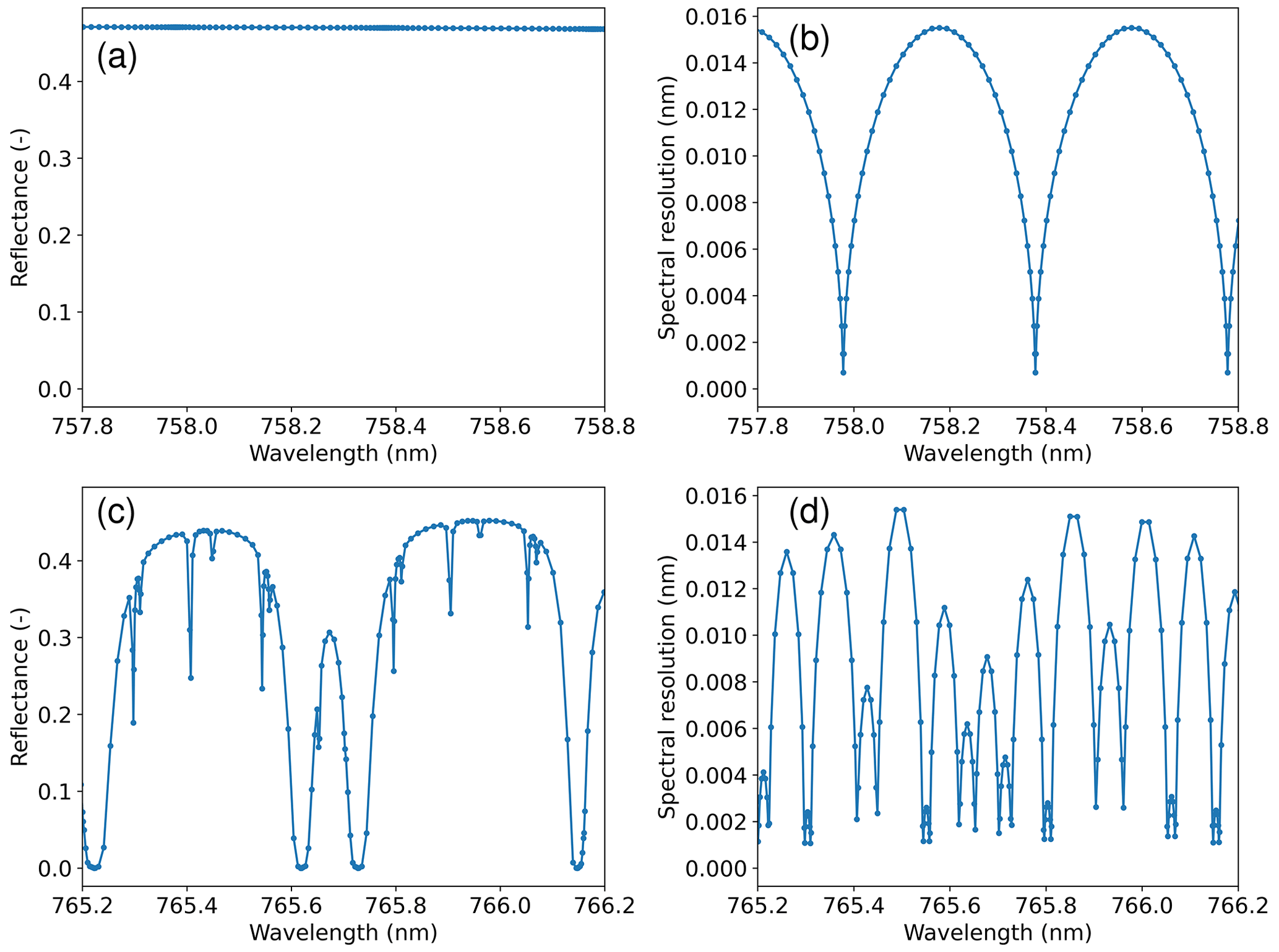
Figure 1Illustration of the wavelength grid used in DISAMAR. (a) Simulated reflectance spectrum at the top of the atmosphere in the continuum part of the oxygen A-band, from 757.8–758.8 nm, at a Gaussian wavelength grid. (b) Wavelength grid interval distribution for the spectrum of (a). Panels (c, d) are similar to panels (a, b) but for the oxygen A-band absorbing part, i.e. 765.2–766.2 nm. In determining the Gaussian wavelength grid, the positions of the absorption lines are taken into account. The number of Gaussian division points is 40 and the minimum number is 8.
Figure 1 shows two 1 nm wide parts of the O2 A-band spectrum, from 757.8 to 758.8 and from 765.2 to 766.2 nm, simulated using DISAMAR. The used spectral resolution (wavelength difference between two grid points) is also shown in Fig. 1. In the spectral part from 757.8 to 758.8 nm, which is devoid of O2 absorption lines, the wavelength intervals are 0.4 nm, and every interval is divided into 40 Gaussian points (see Fig. 1a, b). In the spectral part from 765.2 to 766.2 nm, which has many O2 absorption lines, the intervals are smaller due to the absorption lines (see Fig. 1c, d).
Vertical profiles of absorbing gases are specified using the volume mixing ratio (VMR, in parts per million by volume, ppmv) at pressure grid levels. The volume mixing ratio has the advantage that it remains constant if the temperature changes. The number density of gas molecules is calculated internally using hydrostatic equilibrium. The pressure profile and temperature profile grid can be different for simulation and retrieval: for example, trace gas profile retrievals may be using 50 grid points for the simulation to have high forward model accuracy but only 12 or 18 grid points for the retrieval to represent the limited information content of the measurements.
3.2.2 Cloud and aerosol layers
Two different types of cloud and aerosol layers are distinguished in DISAMAR: an opaque Lambertian reflector and a layer of scattering particles. For the Lambertian type, the cloud and aerosol reflector is located at the top of a pressure interval. For the scattering particles layer, a Henyey–Greenstein phase function or a Mie phase function (or phase matrix in case of polarization) can be used for aerosols and clouds in DISAMAR. If the Henyey–Greenstein phase function is used, the wavelength dependence of the optical thickness is modelled using the Ångstrøm exponent and the absorption is controlled by the single-scattering albedo of the aerosol and cloud particles. A Mie phase function is provided in the form of expansion coefficients (De Rooij and Van der Stap, 1984) in an external file. It is assumed that in general a part of the pixel is cloud-free and that a part is covered by cloud. This part is controlled by the cloud fraction, which can have values in the interval [0, 1].
In DISAMAR the atmosphere is vertically divided into pressure intervals. The surface pressure (e.g. 1000 hPa) defines the lower boundary of the first interval. The intervals are further specified by the pressures of the top of the intervals. For example, if the pressure levels are specified at 700, 600, and 0.1 hPa, the atmosphere has three intervals: from the surface to 700 hPa, from 700 to 600 hPa, and from 600 to 0.1 hPa. The top of the atmosphere (TOA) is at 0.1 hPa. This division is suited to model a cloud layer with boundaries at 700 and 600 hPa. Internally, the pressure levels are translated into altitude levels assuming hydrostatic equilibrium. The formulae are provided in Appendix C. For this calculation, the temperatures at the pressure levels should be provided in the configuration file.
In order to perform radiative transfer calculations, each interval is divided into a number of homogeneous layers using Gaussian division points for the altitude. For example, the three intervals from the surface to TOA may be divided into layers using 12, 10, and 28 Gaussian division points, respectively. The standard atmospheres can be used as input for the pressure, temperature, and gas mixing ratio profiles.
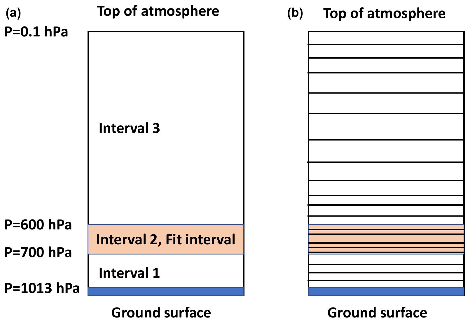
Figure 2Schematic illustration of the altitude grid used in DISAMAR. (a) Pressure intervals in the atmosphere. (b) Each pressure interval is subdivided into layers using Gaussian division points in altitude, which are different per interval. The lowest level is the ground surface, and the highest level is the top of the atmosphere.
Figure 2 illustrates the pressure intervals and the layers in the intervals used in DISAMAR. It is important to use a sufficient number of Gaussian division points for each pressure interval. Each layer is actually further divided into sub-layers using Gaussian division points, with typically four sub-layers per layer. In this way, an accurate integration over altitude can be performed in order to get the layer quantities. Averaging of the optical properties and radiation quantities at the top and bottom of a layer is not sufficiently accurate if the optical properties differ strongly between the top and bottom of the layer. The VMR profiles of gases are interpolated at the radiative transfer model grid. For optically thick clouds, we suggest using 15–50 Gaussian division points for the cloud layer, particularly if the cloud parameters for that layer are to be fitted. For optically thin clouds, 10 Gaussian division points should be sufficient for the cloud layer. We use Gaussian division points because it improves the accuracy in the integration over the altitude.
3.2.3 Surface albedo
The surface below the atmosphere is a Lambertian, i.e. isotropically reflecting, surface. In DISAMAR one can choose between a wavelength-independent surface albedo or a surface albedo that has a polynomial wavelength dependence for each spectral band.
Sun-induced fluorescence from vegetation due to photosynthesis can be observed in the near-infrared spectrum (Joiner et al., 2011; Frankenberg et al., 2011). In order to be able to fit fluorescence in DISAMAR, a polynomial describing surface emission can be used in combination with a wavelength-dependent surface albedo.
3.3 Radiative transfer
3.3.1 Doubling–adding method
The doubling-and-adding method (also called adding method) is described in many books and papers on radiative transfer in planetary atmospheres (e.g. Van de Hulst, 1981; Hansen and Travis, 1974; Hovenier et al., 2004). Here we use the notation that follows De Haan et al. (1987) and Hovenier et al. (2004). We present the new formulae needed to calculate the derivatives; for the detailed formulae used in the doubling–adding method, we refer to De Haan et al. (1987) and Hovenier et al. (2004).
DISAMAR uses the doubling method for the calculation of the scattering properties of the individual atmospheric layers. The adding method is used to add different atmospheric layers, and thus it is used to construct the entire atmosphere. As discussed by De Haan et al. (1987) and Stammes et al. (1989), the doubling–adding method can be used to calculate the internal radiation field at the interface between layers in an efficient manner using principles of invariance. This approach can be extended to obtain the derivatives of the internal radiation field, in a linearization step, with respect to a parameter of the atmosphere–surface system. Because the adding formulae are needed in the derivation of the linearization, we provide them here as well.
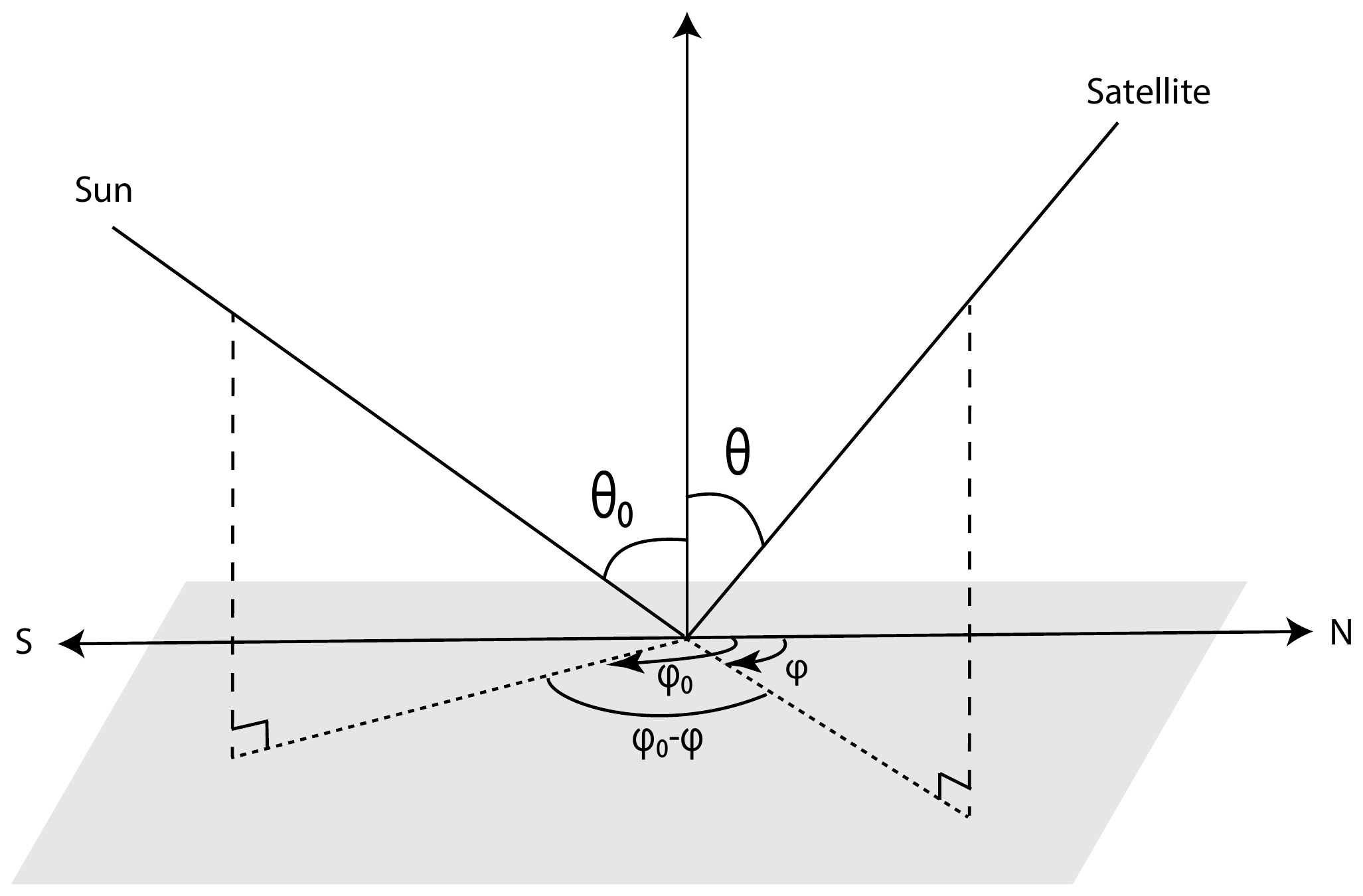
Figure 3Definition of directions in DISAMAR. θ0 and ϕ0 are the solar zenith angle and the solar azimuth angle, respectively, and θ and ϕ are the satellite viewing zenith angle and satellite azimuth angle, respectively. The relative azimuth angle is ϕ−ϕ0. In the super-matrices we use μ0=cos θ0 and μ=cos θ.
Radiative transfer matrices are denoted in bold font, and they operate on incident radiation from right to left. A beam of polarized radiation is represented by the Stokes four-vector . Incident sunlight is the Stokes four-vector , where E0 is the extraterrestrial solar irradiance. The elements of the 4×4 scattering matrix F are expanded into generalized spherical functions, where the expansion coefficients are calculated using the Mie computer program (De Rooij and Van der Stap, 1984). A generalized form of the addition theorem is used to calculate the Fourier coefficients of the 4×4 phase matrix, denoted by Z. Z is found by rotating F to the local meridian plane of incident and scattered light, respectively. Figure 3 illustrates the definition of the directions used in DISAMAR.
3.3.2 Radiation quantities for an optically thin layer
The doubling method is started with an optically thin layer, with an optical thickness of, e.g. . For a thin layer, the Fourier coefficients (indicated by m) of the reflection matrix Rm and the transmission matrix Tm of the layer illuminated at the top are given by
If the thin layer is illuminated at the bottom, the reflection and transmission matrix Fourier coefficients are given by
Here ksca is the volume scattering coefficient of the layer, z is the altitude, and μ and μ′ are the cosines of the polar angles for scattered and incident light, respectively. The “*” indicates quantities with illumination at the bottom. are the Fourier coefficients of the phase matrix of the layer. We assume that the scattering matrix does not depend on altitude within a homogeneous layer The unit of ksca is per kilometre if z is in kilometres.
Attenuation of an incident beam of light due to extinction (sum of scattering and absorption) by the thin layer is given by the direct transmission matrix Ethin:
where the volume extinction coefficient is , with kabs(z) as the volume absorption coefficient. is the Dirac delta function, and 1 is the unity matrix. Equation (5) follows from the Lambert–Beer attenuation law by keeping only the linear term of a Taylor series expansion.
3.3.3 Adding method formulae
We now consider adding two layers on top of each other. Let Ek, Tk, and Rk be the matrices representing the Fourier coefficients of the direct transmission, diffuse transmission, and reflection for illumination at the top of layer k, respectively. Here we omitted the Fourier index m for brevity. Similarly, let , , and be these matrices for illumination at the bottom of layer k. The matrices for layer k+1 are denoted similarly. Ek is a diagonal matrix. For a plane-parallel atmosphere, its elements are given by
where i is the index of the Gaussian μ point, is the Stokes parameter index, and τ is the layer optical thickness.
The adding scheme for illumination at the top of the two layers is presented in Eqs. (7)–(12). The adding scheme for illumination at the bottom of the two layers is presented in Appendix B. The adding scheme is used for every Fourier coefficient; at the end of the process, the reflection and transmission matrices are obtained by summing up the Fourier coefficients.
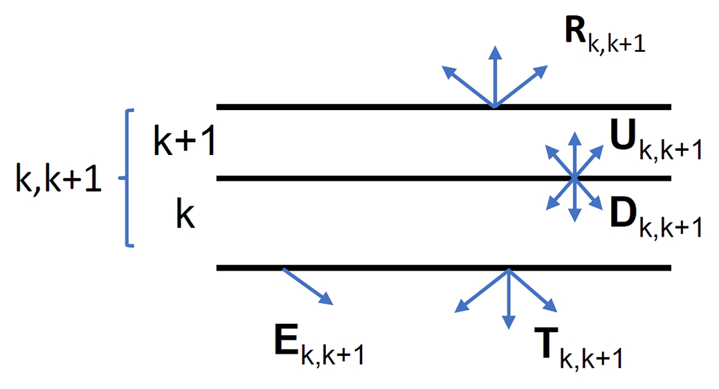
Figure 4Radiation fields after adding two layers, k and k+1, into the adding method. Layer is the combined layer. and are the upward and downward diffuse internal fields for the combined layer. and are the reflection and diffuse transmission of the combined layer. is the combined direct transmission (direct attenuation).
The scheme of adding layer k+1 on top of layer k to create a combined layer is illustrated in Fig. 4. The adding method formulae are as follows.
Here is the attenuation of incident light by the combined layer. is the sum of the repeated reflections between the layers for a unit amount of light incident on the interface between the layers. is the diffuse downward light at the interface between the layers, is the upward light at the interface between the layers, is the reflectance of the combined layer, and is the transmission of the combined layer.
The matrices R, T, E, Q, D, and U are so-called super-matrices. The elements of super-matrices contain Gaussian points for the polar angle with weights that are suited for numerical integration by multiplication of two super-matrices. For the definition of super-matrices, we refer to De Haan et al. (1987). The total number of polar angles, Nμ, is the number of Gaussian division points, Ng, plus one solar zenith angle and one viewing zenith angle, pertaining to the selected sun-view geometry. The dimension of the super-matrix is (Nμ, Nμ) if polarization is ignored and (4Nμ, 4Nμ) if polarization is included using all four Stokes parameters. In the following a super-matrix is meant when we speak of a matrix.
The formula for repeated reflections at the interface, Eq. (8), can also be written as
where 1 is the unity matrix. Inserting Eq. (13) into Eq. (9) yields
Equations (13) and (14) are needed in the derivation of the derivatives, as will be discussed next.
3.3.4 Derivatives of the reflectance using the adding method
Retrieval algorithms that are designed to derive quantitative information about properties of the atmosphere from measured spectra require not only an atmospheric model but also derivatives of the reflectance with respect to the optical properties of the atmosphere, sometimes called Jacobians or weighting functions (see, e.g. Spurr, 2006; Hasekamp and Landgraf, 2005; Bai et al., 2020; Rodgers, 2000), to simulate reflectance spectra. Obviously, these derivatives can be calculated using numerical differentiation based on perturbation. However, numerical differentiation is a slow process, in particular when altitude profiles have to be determined and the atmosphere consists of 20–100 layers. Here we derive semi-analytical expressions for the derivatives of the reflectance with respect to the optical properties of the atmospheric layers. The semi-analytical derivatives are calculated at the interfaces of the layers, i.e. at levels. The derivatives for the layers themselves can then be calculated from the derivatives at the interfaces using interpolation and integration over the layers. Note that often the derivatives are calculated pertaining to optical properties of atmospheric layers, which differs from our approach.
The derivatives can be found by calculating the change in reflectance at top-of-atmosphere using the changes in atmospheric properties at each height, . In the adding scheme, such a change can be invoked by adding a thin layer at altitude z. As shown by Eqs. (1)–(5), the reflection and transmission of a thin layer can be written analytically as a function of the optical properties of the layer: ksca, kabs, and Z. Therefore, the computation of semi-analytical derivatives should involve a thin layer. If one first calculates the reflection of two layers on top of each other, Rtop+bot, and next calculates the reflection of the two layers with a thin layer in between, , then can be calculated from the following differential: (.
We divide the atmosphere into two parts, a top part and a bottom part. Let Rtop, , Ttop, be the Fourier coefficients of the reflection and transmission matrices of the top part; the quantities without an asterisk denote the properties for illumination at the top, and the quantities with an asterisk denote illumination at the bottom. Similarly, matrices with the subscript “bot” denote the properties of the lower part of the atmosphere.
Using the adding formulae, Eqs. (7)–(12) and keeping only constant terms and terms linear in dz, one can derive the derivative in a concise form as follows:
where Q and Q* are given by
and W(z) is given by
Here is the super-matrix with the element on the diagonal, representing the slant path for extinction. are abbreviated notations of , the super-matrices of the Fourier coefficients of the phase matrix. The full derivation of Eq. (15) is given in Appendix A.
Inserting Eq. (18) into Eq. (15) yields the separate terms of the derivative:
Since we want to calculate the derivative with respect to the scattering and absorption properties of the atmosphere at altitude z, Eq. (19) has to be expressed in the internal fields D and U at altitude z. Therefore, in Eqs. (20)–(23) the internal fields are expressed using (1+Q) or () and R, T, and E. The relations are as follows.
Here indicates the transpose of a super-matrix, and is a diagonal matrix that occurs due to polarization. By replacing the terms related to (1+Q) and () in Eq. (19) with the relations in Eqs. (20)–(23), we obtain the derivative in terms of the internal radiation fields:
First, replace kext with ksca+kabs in Eq. (24) and separate the terms containing kabs and ksca. Following this, calculate the partial derivative of with respect to kabs and ksca using Eq. (24). This gives the partial derivative of the reflectance with respect to the volume absorption coefficient (Eq. 25) and the partial derivative of the reflectance with respect to the volume scattering coefficient (Eq. 26). These equations are as follows:
The above relation, Eq. (26), is a generic expression for the derivative with respect to the volume scattering coefficient. However, since it contains the phase matrix, it makes a difference whether the change in the volume scattering coefficient is due to a change in the number of scattering molecules in the thin layer or due to a change in the number of aerosol particles. If the number of scattering molecules is changing, the phase matrix of the molecules has to be used in Eq. (26), whereas the phase matrix of the aerosol particles has to be used if the number of aerosol particles is changing. In general one has to distinguish between molecules, aerosols, and cloud particles.
3.3.5 Derivatives of the reflectance with respect to specific parameters
If polarization is ignored, the partial derivative of the reflectance with respect to some specific quantity x(z) (e.g. ozone number density or aerosol number density) can be expressed as follows:
where R is the (1, 1) element of R and is the phase matrix expansion coefficient for unpolarized light. In DISAMAR the third term on the right-hand side is ignored, so it is assumed that the phase matrix of the particles does not change as function of z. The derivatives for specific parameters can be calculated using these basic derivatives (De Haan, 2012). Here we give two examples of the use of the semi-analytical derivatives presented in the previous section.
The first example is the altitude-resolved air mass factor (also called block air mass factor) at wavelength λ, m(z,λ). The altitude-resolved air mass factor is used in DOAS retrievals and represents the relative reduction in the reflectance when a unit amount of absorption is added to the atmosphere in a thin layer located between z and z+dz. So it is the partial derivative of the reflectance due to the absorber at z divided by the reflectance. Writing the reflectance of the atmosphere without the extra absorption as R(λ,0), the altitude-resolved air mass factor is defined as follows:
The partial derivative on the right-hand side can now be calculated from Eq. (25).
The second example is the derivative of the reflectance to the altitude of a Lambertian cloud below an absorbing and scattering gas layer:
Here the cloud is approximated as a Lambertian surface, without any transmission. When the altitude of the Lambertian cloud increases, the amount of gas above the cloud is reduced, and thus we get a minus sign in Eq. (29). The amount of scattering gas that is removed is proportional to the volume scattering coefficient (kgas,sca), whereas the amount of absorbing gas that is removed is proportional to the volume absorption coefficient (kgas,abs). The partial derivatives on the right-hand side of Eq. (29) can now be calculated from Eqs. (25) and (26).
As noted before, the derivatives can also be calculated numerically. Thus, , with xk element k of the state vector x, is written as the following numerical differential:
Here Δx=0, except for the element k, where Δx=Δxk. By comparing the analytical derivatives in DISAMAR with the numerical derivatives, we can validate the former.
3.3.6 Layer-based orders of scattering method (LABOS)
In the adding method as implemented in DISAMAR, the reflection matrix is calculated for a set of solar directions equal to the number of Gaussian division points used for integration over the polar angle plus at least two additional directions, namely the actual viewing direction and the actual solar position. Thus, for satellite retrievals the adding method provides more results than required.
The layer-based orders of scattering method (LABOS) has been developed to obtain the reflection matrix for the actual solar position or, when derivatives are required, for the actual solar position and a solar position corresponding to the viewing direction. The reflection and transmission properties of the individual homogeneous layers are still calculated with the doubling method; only the adding of different layers and the subsequent calculation of the internal field is replaced by the successive orders of scattering method (see Eqs. 35–38). Here an order of scattering represents scattering by an atmospheric layer. This differs from the classical method of successive orders of scattering where the scattering element is a volume element of the atmosphere instead of a layer (Lenoble et al., 2007; Min and Duan, 2004). In the adding method, one deals with matrix–matrix multiplications, whereas in LABOS one deals with matrix–vector multiplications. However, in LABOS the calculations have to be repeated for the different orders of scattering. Hence, for an optically thin atmosphere with only a few orders of scattering, LABOS requires less calculation time, while adding is more efficient for optically thick atmospheres, e.g. those containing clouds.
In LABOS we deal with the upward and downward internal radiation fields, i.e. U and D. In order to determine the derivatives using reciprocity, we need to consider two directions for the incident light, one corresponding to the actual solar position and one corresponding to the viewing direction. Therefore, U and D are (4N, 2) matrices, with the first column corresponding to incident light for the viewing direction, and the second column corresponding to the solar direction, where the number of polar angles . If the incident light is polarized, we need (4Nμ, 8) matrices. In order to calculate the total internal fields U and D (see Eqs. 35–38), we first need to calculate local internal fields Ulocal and Dlocal (see Eqs. 31–32).
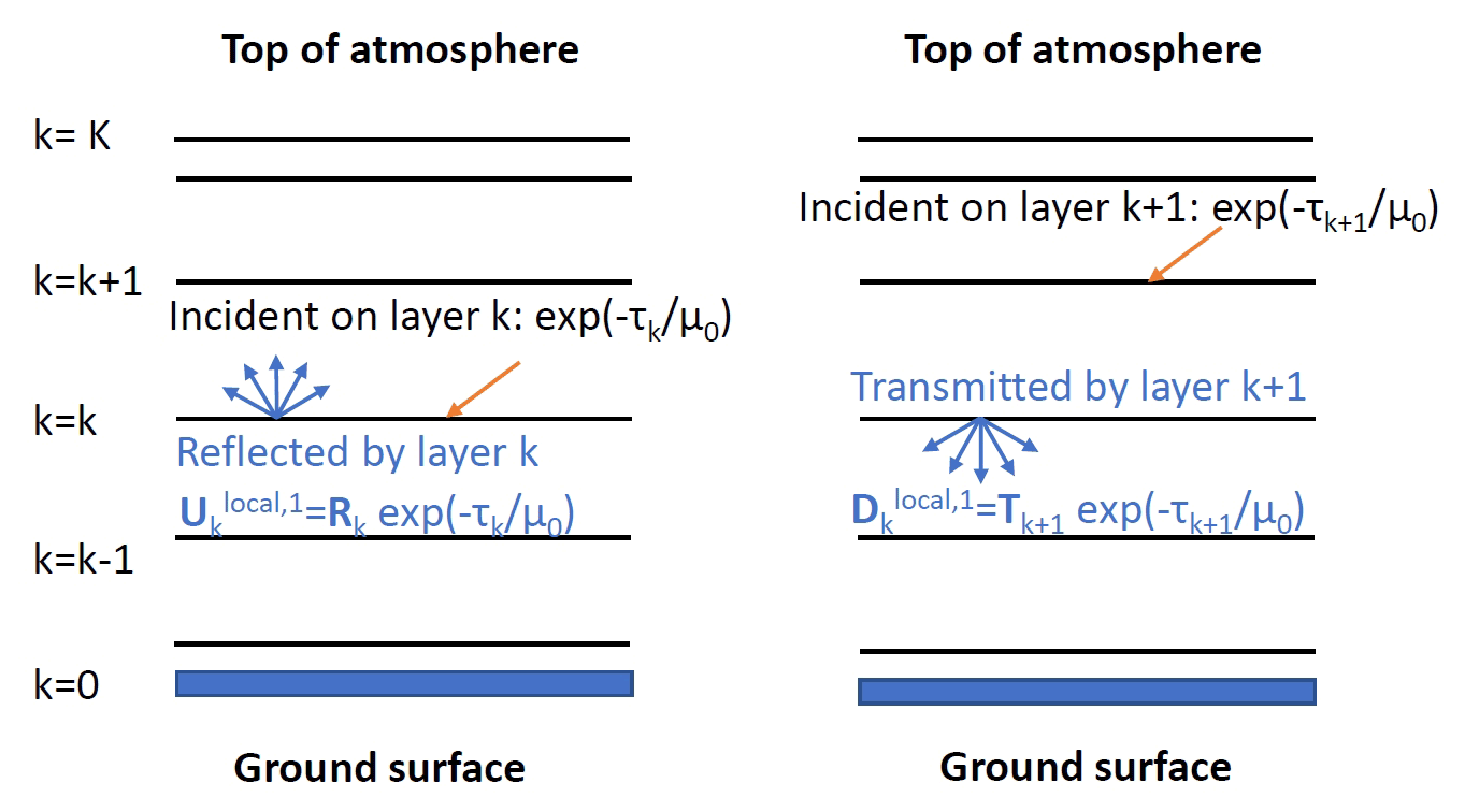
Figure 5Illustration of the principle of the LABOS method, showing the local upward and downward first-order scattering radiation fields at level k. The index indicates the level, where k=0 is the surface and k=K is the top of the atmosphere. The layer number refers to the upper level of the layer, and thus layer k is located between levels k−1 and k.
Let Rk and Tk be the super-matrices for the reflection and transmission of layer k (). If k=0, the reflection matrix is that of the surface, and the transmission matrix vanishes. Further, let μ and μ0 be the cosines of the viewing and solar zenith angle, respectively. In order to evaluate different orders of scattering, we first consider the so-called local radiation field, which is due to the reflection by the layer just below the level considered and the transmission by the layer just above this level. Figure 5 illustrates the local upward and downward radiation fields at the interface k for the first-order scattering (n=1).
The local upward first-order radiation at level k is given by
where τk is the vertical optical depth of level k, measured from the top of the atmosphere. The two columns of matrix correspond to the two columns of super-matrix Rk having indices 4Ng+1 and , respectively, if the dimension of the Stokes vector is 4. The first-order local downward radiation field at level k is
Here the two columns of correspond to the two columns of super-matrix Tk+1 with indices 4Ng+1 and 4Ng+5. The superscript 1 denotes the first-order scattering for the layers.
From the local radiation fields, we can now derive the total radiation fields. The first-order-scattered upward radiation at level k, , is calculated as the sum of the contributions of the local upward radiation from the ground up to level k. The downward radiation at level k, , is calculated as the sum of the contributions of the local downward radiation from level k up to level K (TOA):
where the attenuation accounts for the direct transmission of light from level l to level k. We note that Eqs. (33) and (34) can be rewritten in terms of the following recurrence relations, which are more efficient to evaluate.
The same recurrence relations hold for the higher orders of scattering because the direct transmission of radiation to other levels is the same for each order of scattering.
The following equations are used to determine the local radiation fields for the higher orders of scattering, where n indicates the order of scattering:
where is the reflection of layer k+1 for illumination at its bottom. Since the layers are homogeneous, we can use symmetry relations to calculate and from Rk+1 and Tk, respectively (Hovenier et al., 2004). After the local radiation fields are calculated using Eqs. (39) and (40), the recurrence relations are applied for the transfer to other levels to provide the radiation fields and for scattering order n+1.
One can continue calculating the orders of scattering and summing them up until the contribution of higher orders can be ignored. At the end of the calculation, the internal radiation fields at all levels are known. The Fourier coefficients of the upward radiation at the top of the atmosphere provide the reflection, and the internal radiation fields are used to calculate the derivatives. In DISAMAR users can choose to use either the doubling–adding method or the doubling–LABOS method.
3.3.7 Reflection calculated by integration over the source function
The upward radiation at the top of the atmosphere is calculated by assuming that the atmosphere is consisting of homogeneous layers, both in the doubling–adding method and in the doubling–LABOS method. The calculation will converge to the correct value if many homogeneous layers are used to represent the true atmospheric scattering and absorption profile. In DISAMAR the reflection can also be calculated from numerical integration over the source function J to mitigate errors due to layering that is too coarse. The reason is that by using the source function the assumption of homogeneous layers is not used for single scattering but only for multiple scattering. For each azimuthal Fourier term the reflection is then given by
where the surface is at z=0. Since the source function for the surface is a Dirac delta function in z, its contribution to the reflection occurs as a separate term in Eq. (41). The source function for the atmosphere is
and are the internal fields at altitude z that are known after doubling–adding or doubling–LABOS calculations. Hence, J can be easily calculated at those altitudes where the internal radiation fields are known.
Three retrieval methods are implemented in DISAMAR: the optimal estimation (OE), differential optical absorption spectroscopy (DOAS), and differential and smooth absorption separated (DISMAS) methods.
The OE method is implemented in DISAMAR following Rodgers (2000). The OE method can be used for various retrievals implemented in DISAMAR, especially ozone profile retrieval (Kroon et al., 2011) and aerosol layer height retrieval (Sanders et al., 2015; Nanda et al., 2018). The OE output includes the retrieved parameters and their error matrices, correlations, gain matrices, and averaging kernels.
The DOAS method is described in the literature (Platt and Stutz, 2008). Below we describe the DISMAS method, which is related to the DOAS method, in detail.
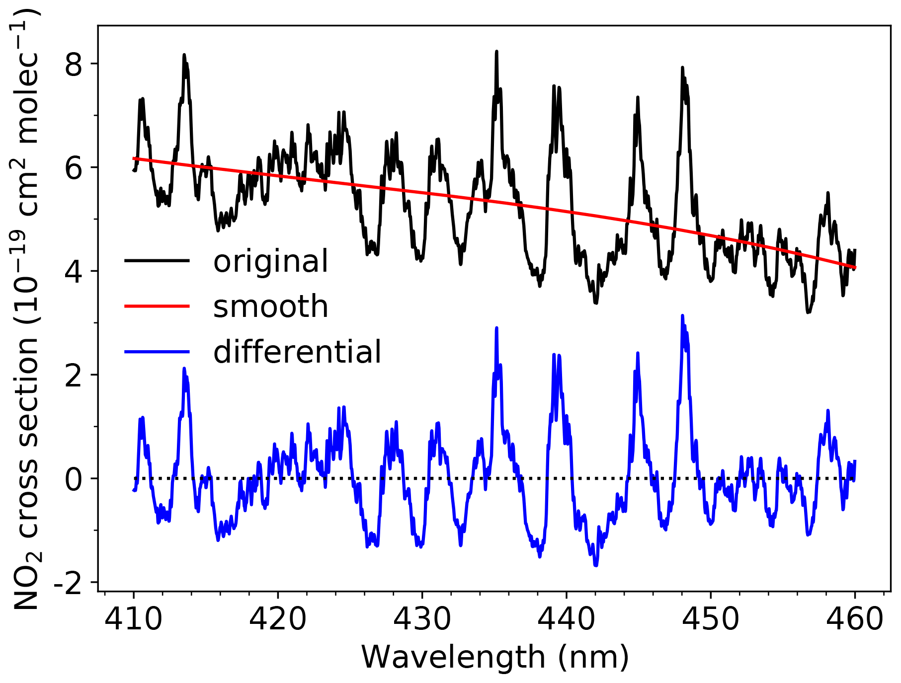
Figure 6Illustration of the principle of DISMAS using the NO2 cross section as an example. The NO2 cross section is separated into two parts: a smooth part, using a fit of a third-order polynomial, and a differential part. The radiative transfer calculations are performed for the smooth part at a few selected wavelengths where the differential cross section is vanishing.
4.1 DISMAS method
The DISMAS method uses the principle of DOAS for the forward simulation of spectra and the OE method for the retrieval. Therefore, the DISMAS method reduces the forward simulation time, making it faster than a full forward simulation, but still provides the full error estimation as in OE. DISMAS can be used for the retrieval of total columns of weakly absorbing gases, like O3 (in the visible wavelength range), NO2, SO2, BrO, and CH2O, but not for strong absorbers, such as O2, H2O, CH4, CO, and O3 (in the UV). In DISMAS, gas absorption spectra are separated into a smooth part and a differential part, which is similar to DOAS. As an illustration, Fig. 6 shows an NO2 absorption spectrum with a smooth and a differential absorption part.
For the reflectance spectrum around a weak atmospheric absorption line, e.g. from NO2, one can use the Lambert–Beer attenuation law as follows:
where R(λ,0) is the reflectance of the atmosphere without the absorbing gas, M(λ) is the air mass factor (AMF) of the total atmosphere (unitless), is the altitude-averaged (subscript a) absorption cross section (in ), and N is the vertical column density of the absorbing gas (in ). Introducing the smooth absorption cross section, , and the differential absorption cross section, , one obtains
Here and M(λ) are smooth functions of wavelength, which are calculated with a radiative transfer model at a few wavelengths and are fitted as a function of wavelength to be interpolated to a high-resolution wavelength grid. The differential term
varies strongly with wavelength and has to be evaluated at a high-resolution wavelength grid. However, this analytical formula can be calculated very quickly without the need to solve the radiative transfer model. The smooth functions and M(λ) are calculated at those wavelengths, λp, where the differential absorption cross sections are zero because at those points (see Eq. 44)
Hence, radiative transfer calculations for a small number of wavelengths λp are sufficient to determine the reflectance spectrum at a high spectral resolution grid.
To simulate a measured spectrum in DISMAS, the modelled reflectance spectrum on the high-resolution grid is multiplied with a high-resolution solar irradiance spectrum and convoluted with the instrument's spectral response function (or slit function). This provides a simulated radiance spectrum of the instrument that can be compared to an actually measured radiance spectrum. In practice, the simulated radiance spectrum is divided by the simulated irradiance spectrum to eliminate common errors, and the logarithm of the reflectance is used for fitting.
The air mass factor M(λ) can be calculated from m(z,λ), which is known from the radiative transfer calculations (see Eq. 28):
where n(z) is the number density profile of the absorbing gas. To start the optimal estimation process in DISMAS, m(z,λ) is initialized using a geometrical air mass factor. In subsequent iteration steps, the value of m(z,λ) is updated by radiative transfer calculations for the new atmospheric composition state vector.
If there is more than one absorbing trace gas in a fit window, one can use the slant absorption optical thickness, , instead of the absorption cross section to separate the smooth and differential parts of the absorption spectrum.
For fitting the modelled reflectance to the measured reflectance and determining the errors in the retrieved parameter values, the derivatives are needed. Here we give the derivatives with respect to the total column of a trace gas and to the cloud fraction for a partly cloudy pixel.
For a partly cloudy pixel with K different trace gases, the reflectance is written as follows:
where c is the cloud fraction, subscript “sm” refers to the smooth reflectance, and superscripts “clr” and “cld” denote the clear and cloudy part of the pixel, respectively. The derivative with respect to the cloud fraction is
The derivative with respect to the total column of trace gas k, Nk, becomes
where we assume that the air mass factor does not change significantly when the column changes, which is accurate for weak absorption.
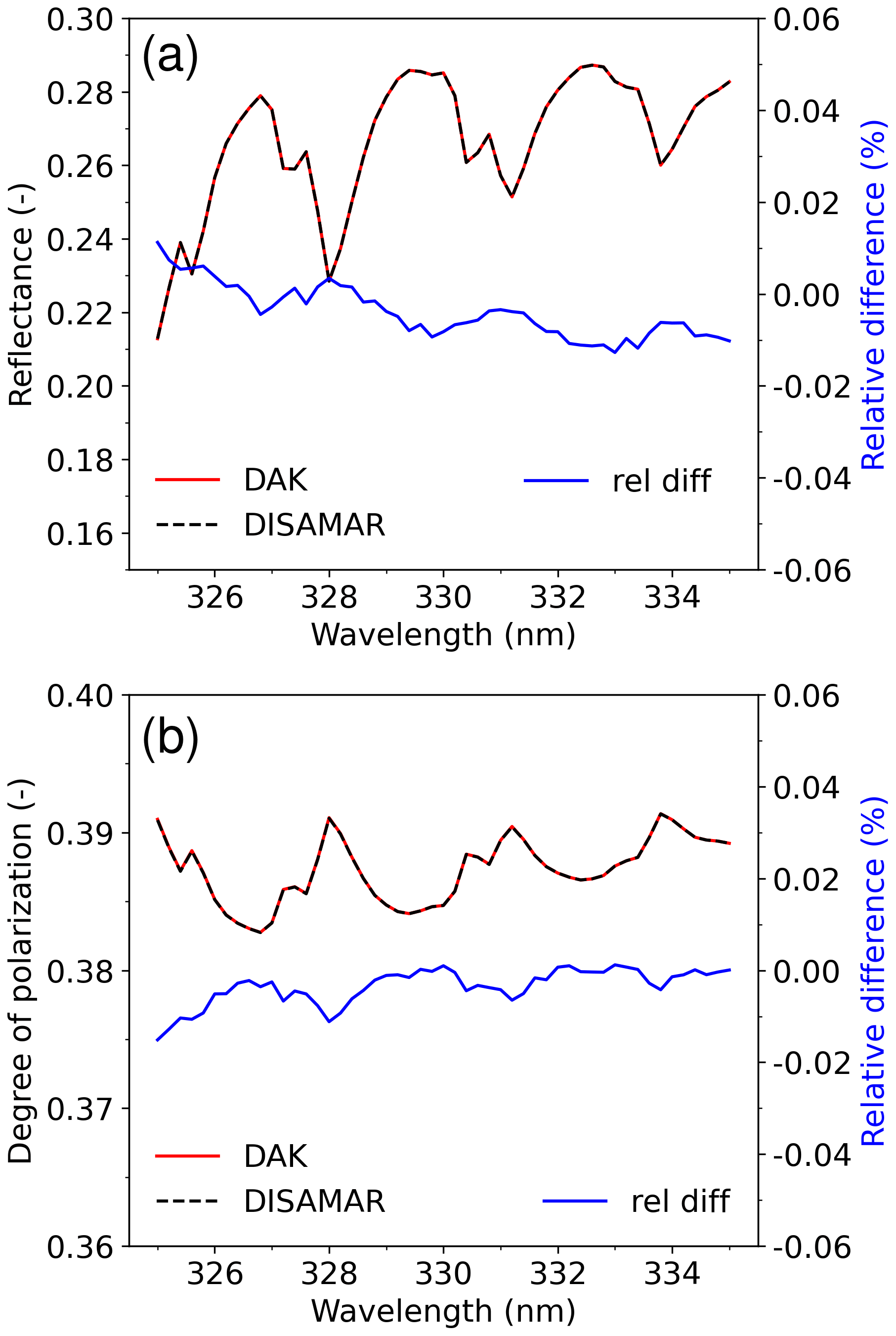
Figure 7Comparison of DISAMAR and DAK simulations of TOA reflection spectra between 325 and 335 nm: (a) reflectance and (b) degree of linear polarization. The relative difference is defined as (DISAMAR−DAK) / DAK (in percent). The wavelength step in the spectra is 0.2 nm, and no ISRF convolution is performed. The geometry is as follows: nadir view with a solar zenith angle of 60∘. Surface albedo is 0.02.

Figure 8(a) Derivative of the reflectance to the cloud height, , for a scene with a Lambertian cloud, calculated using the semi-analytical method (Eq. 29) and the numerical method. The derivative is normalized to the maximum value calculated using the numerical method. (b) Relative difference (in percent) between semi-analytical and numerical derivatives. The steep change in the relative difference at 758 nm is caused by the fact that the derivative is very small where the O2 absorption approaches zero. The geometry is as follows: nadir view with a solar zenith angle of 30∘. The cloud fraction is 1, and the Lambertian cloud albedo is 0.8.
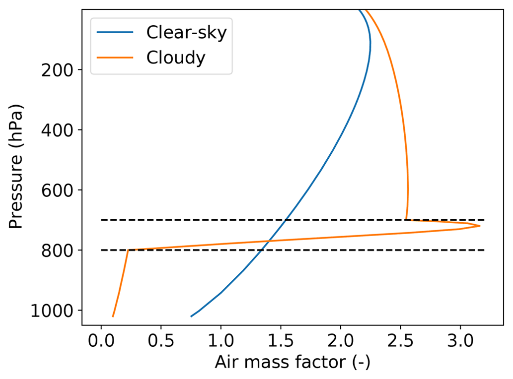
Figure 9Altitude-resolved air mass factor of NO2 at 440 nm for a cloudy scene and a clear-sky scene. The scattering cloud layer is located between 700 and 800 hPa with a cloud optical thickness of 10. The dashed lines indicate the cloud top and base pressure. The surface albedo is 0.05. The geometry is as follows: nadir view with a solar zenith angle of 30∘.
5.1 Comparison with the Doubling–Adding KNMI (DAK) model
As an example, we show a comparison of DISAMAR with the DAK radiative transfer model (De Haan et al., 1987; Stammes et al., 1989) for the simulated reflectance and linear polarization spectrum of a Rayleigh scattering atmosphere in the ozone Huggins band region between 325 and 335 nm; see Fig. 7. In DISAMAR we used the doubling-adding method in order to get the best agreement with DAK. The atmospheric temperature, pressure, and ozone mixing ratio profiles are taken from the mid-latitude summer atmosphere (Anderson et al., 1986). Since DISAMAR uses the hydrostatic relation to calculate altitude with the input pressure and temperature profiles, the altitude in DAK is corrected for the hydrostatic relation. This correction is important to obtain the same Rayleigh scattering optical thickness in this wavelength range. The total ozone column is 335.66 DU in DAK and DISAMAR. The ozone cross section was taken from Bass and Paur (1985) because these data are available in both DAK and DISAMAR.
Figure 7 shows the simulated reflectance, degree of linear polarization, and the corresponding relative differences, for the viewing and solar geometry μ=1, μ0=0.5. DISAMAR and DAK agree very well for the simulated reflectance and degree of linear polarization, with absolute differences of less than 0.01 %. DISAMAR and DAK use different internal wavelength grids, altitude grids, and interpolation methods, which may explain the remaining small differences.
5.2 Derivatives
The accuracy of the semi-analytical formulae for the derivatives based on the adding method is checked here by comparison with the numerically calculated derivatives. We show an example of the derivative of the cloud height, , in the O2 A-band for a Lambertian cloud. In the calculation, the atmospheric profile is mid-latitude summer, the cloud fraction is set to 1, and the cloud albedo set to 0.8. The viewing and solar geometry is μ=1, μ0=0.8660. The spectrum of the derivative is calculated at a high-resolution wavelength grid and convolved with a Gaussian ISRF with a FWHM of 0.4 nm. As shown in Fig. 8, the semi-analytical and numerical derivatives are very similar: the mean relative difference is −0.13 %. At 758–759 nm, the O2 absorption is very small, about 100 times smaller than in the absorption band close to 760–761 nm. The spectrum of clearly shows that the cloud height information comes from the absorption band. If the cloud fraction is smaller than 1, the derivative is also smaller because the radiance is smaller. Although the relative difference between the semi-analytical and numerical derivatives behaves steeply in the continuum at 758–759 nm, it is still within 0.2 % over the entire absorption band. Therefore, the semi-analytical derivatives are considered accurate for cloud height retrievals.
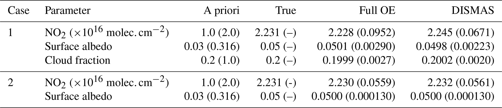
Table 1Comparison between DISMAS and full optimal estimation (OE) retrievals of the total NO2 column in a partly cloudy scene (cloud fraction 0.2, Lambertian cloud albedo 0.8) with a reflecting surface. In Case 1 all three parameters are retrieved, whereas in Case 2 the cloud fraction is fixed and only NO2 column and surface albedo are retrieved. The a priori and retrieval errors are given between brackets.
The altitude-resolved AMF, m(λ,z), is used in the DOAS algorithm to convert the slant column density of a gas to the vertical column density (see Sect. 3.3.5). The altitude-resolved AMF was calculated using Eq. (28), and the semi-analytical partial derivatives are taken from DISAMAR. It can also be calculated numerically, but that method is slower and requires a finer altitude grid to get accurate results. Figure 9 shows the altitude-resolved AMF of NO2 calculated using the semi-analytical derivatives for a cloudy scene and a clear-sky scene. Here the atmospheric profile and NO2 mixing ratio are taken from the mid-latitude summer atmospheric profile. A scattering cloud layer is specified between 800 and 700 hPa with a Henyey–Greenstein phase function, asymmetry parameter 0.85, and single scattering albedo 1.0. The cloud optical thickness is 10. The surface albedo is 0.05. The viewing and solar geometry is μ=1, μ0=0.8660.
Figure 9 shows that inside the cloud the AMF has a peak close to the cloud top due to the enhancement from multiple scattering. Above the cloud top, the AMF is larger than the clear-sky AMF due to the bright cloud layer. Below the cloud top, the AMF decreases and becomes smaller than the clear-sky AMF. At TOA, the AMF for both scenes approach the geometric AMF, , which is 2.155 for this case. These are typical characteristics of the altitude-resolved AMF of NO2.
5.3 Comparison of DISMAS and full OE for NO2 retrievals
The DISAMAR code can simulate the retrieval of total columns of trace gases, ozone profile, cloud layer height, aerosol layer height, cloud (or aerosol) optical thickness, surface albedo, and surface pressure. Some OE retrieval applications were mentioned in the introduction of Sect. 4. Because the DISMAS retrieval approach is new and not used operationally, we show the DISMAS results for NO2 column retrieval in a cloudy scene here as an example. The scene in the simulation is constructed as follows: the atmosphere is a typical European polluted model, the cloud is a Lambertian cloud with a fixed albedo of 0.8 located at 4 km altitude, and the geometry is nadir view with solar zenith angle 60∘. In the retrieval, the fitting window is 420–450 nm. Radiative transfer calculations are performed at four wavelengths for DISMAS and at about 900 wavelengths for OE. Thus, DISMAS enables a large reduction of the number of radiative transfer calculations needed for spectral fitting. Table 1 shows the comparison between DISMAS and full OE for the NO2 retrievals for two cases. In Case 1, three parameters are retrieved: NO2 total column density, surface albedo, and cloud fraction. In Case 2, the cloud fraction is fixed, and only the NO2 total column density and the surface albedo are retrieved.
The parameters were accurately retrieved by both methods. The error estimates for the retrieved surface albedo and cloud fraction differ only little, but DISMAS underestimates the error in the retrieved NO2 column.
If the cloud fraction is fixed to its true value (0.20) so that the NO2 column and the surface albedo are the only fit parameters, DISMAS and OE fully agree for the errors in the NO2 column, while the surface albedo values are also the same.
From our results, we find that DISMAS and OE are functionally equivalent for weak absorption, except that the error in the retrieved column may differ in some cases. The main advantage is that DISMAS is much faster than full OE, which might make operational use of DISMAS attractive. This would make it possible to derive the surface albedo and the cloud fraction directly from the measured radiance in the NO2 window, thereby reducing the bias of the retrieved NO2 column significantly.
The aim of the DISAMAR code is to determine instrument specifications and analyse methods for retrievals of atmospheric composition from satellite observations in the range of 270–2400 nm. We have described the principles of the DISAMAR radiative transfer model and its innovative retrieval capabilities. The novel features in DISAMAR are the semi-analytical derivatives of the reflectance using the internal radiation field, the layer-based orders of scattering method LABOS, which speeds up the calculations, and the DISMAS retrieval method, which reduces the number of radiative transfer calculations in DOAS-type retrievals. The semi-analytical derivatives are based on the linearization of the adding method, which is detailed in Appendix A. Other features of DISAMAR that improve the accuracy of forward modelling are the Gaussian grids for height and wavelength and the integration over the source function to obtain the reflectance.
DISAMAR can be used as an accurate radiative transfer model for simulations and as a retrieval algorithm for several applications. We have given a few examples of applications, namely forward modelling of the polarized reflectance in the UV, the derivative of cloud height in the O2 A-band, and an application of DISMAS for NO2 retrieval in a cloudy scene. It is shown that for retrieval of total columns of weak absorbers, DISMAS has a similar functionality to optimal estimation but is much faster.
In the past few years DISAMAR has been used extensively in trace gas, aerosol, and cloud retrieval studies for OMI, TROPOMI, Sentinel-4, and Sentinel-5. DISAMAR is currently being used for operational retrievals of ozone profiles from UV spectra for OMI (Kroon et al., 2011) and TROPOMI (Veefkind et al., 2021) and aerosol layer height retrieval from the O2 A-band for TROPOMI (Nanda et al., 2019). More applications of DISAMAR are described in the DISAMAR algorithm document (De Haan, 2012), and can be found in the peer-reviewed literature; for example, on the role of aerosols in retrievals of NO2; see Castellanos et al. (2015) and Chimot et al. (2016, 2017).
Currently, DISAMAR is still under development and has certain limitations: Raman scattering in water (Vasilkov et al., 2002) is ignored, remote sensing from the ground and from aircraft is not supported, and limb observations are not supported. Furthermore, the radiative transfer part assumes a plane-parallel atmosphere, albeit with a correction for the curvature of the atmosphere for incident sunlight (pseudo-spherical correction; see Appendix B). This may become inaccurate for observations far from the nadir (viewing zenith angle ), in particular for stratospheric gases (Spurr, 2002). In the coming years DISAMAR will be further extended and used to develop optimized retrieval algorithms, including those using neural networks (Nanda et al., 2019).
Here we derive the formulae for the derivative of the reflection, , given by Eq. (15) in Sect. 3.3.4, by means of linearization of the adding equations. To that end, we divide the atmosphere into two parts, a top part and a bottom part. Let Rtop, , Ttop, and be the Fourier coefficients of the reflection and transmission matrices of the top part. The quantities without an asterisk denote the properties for illumination at its top, while the asterisk denotes illumination at its bottom. Analogously, matrices with the subscript “bot” denote the properties of the lower partial atmosphere. We start with the adding equations Eqs. (11), (10), and (9) and change subscript k+1 to “top” and subscript k to “bot”:
Inserting Eqs. (A2) and (A3) into Eq. (A1), we obtain the adding equation for the reflection at the top in a concise form:
where
We now start the linearization process by adding a thin layer on top of the lower partial atmosphere. Using Eq. (A4) and writing “thin” instead of “top” yields:
The radiation fields for a thin layer have already been given by Eqs. (1)–(5) in Sect. 3.3.2. We observe that Rthin, Tthin, , , and (1−Ethin) are proportional to dz. In the linearization process, we keep only terms that are constant or linear in dz. We note that only the first term of Eq. (A7) has to be kept because the second term is ∝(dz)2. Inserting Eq. (A7) into Eq. (A6) and keeping only terms that are constant or linear in dz, the derivation steps towards the linearized form of Eq. (A6), given by Eq. (A8), are
We now add the upper partial atmosphere to this combined (“thin+bot”) lower layer and derive the linearized expression for given by Eq. (A9.). We start again from Eq. (A4):
Subtracting these two equations we get the difference in R due to the thin layer:
Let us now focus on the term between the square brackets in Eq. (A11). The linearization steps, in which only constant terms and terms linear in dz are kept, are
In step 3, and Qtop+bot are replaced by the first term of their expansions; in step 7, the last term is removed because it depends on (dz)2; in step 8, is approximated by . Because is small, step 8 only introduces a small error. In order to get a compact form, in step 9 a small term, , is added.
Inserting Eq. (A12) into Eq. (A11), we obtain the linearized form of the difference dR:
Here the term contains the optical properties of the thin layer: ksca, kext and Z. This term can be written in terms of these optical properties by using Eq. (A8) and inserting the thin-layer formulae Eqs. (1)–(5).
For the definition of the phase matrix Z′ with special super-matrix weights we refer to De Haan, 2012; De Haan et al., 1987. If we now insert this relation, Eq. (A14), into Eq. (A13), we get the following end result:
This formula, Eq. (A15), is the derivative equation given in Eq. (15).
The pseudo-spherical correction in DISAMAR corrects for the curvature of the atmosphere for incident sunlight. For the other light paths the atmosphere remains plane-parallel. In order to calculate the pseudo-spherical correction, the adding scheme for illumination of the layers from below is implemented. These equations are as follows:
We assume that the individual layers remain plane-parallel; the only correction that is needed for the reflectance is to change the attenuation terms for incident sunlight. For the adding method it means replacing Ek+1, when it occurs on the right-hand side of a term, with a new attenuation term. The pseudo-spherical correction method follows Spurr (2002), and thus the details are not given here.
The partial derivative of the reflectance to the absorption coefficient, Eq. (25) from Sect. 3.3.4, can be rewritten as
With the pseudo-spherical correction, the last term at the right-hand side of Eq. (B6) should be replaced by Eq. (B9). Equations (B7)–(B9) present the derivation of the pseudo-spherical correction:
where RE is the radius of the Earth in kilometres and zk and zl are the altitudes (in kilometres) of levels k and l, respectively. Here we use the local value of U to distinguish between the different levels below level k. The factor occurs in Eq. (B7) because we used the transpose of U; this is also the reason for the order of the arguments for . The sum over n is the sum over the orders of scattering. For a plane-parallel atmosphere, Eq. (B7) can be written as Eq. (B8). For a spherical atmosphere, should be replaced by , noted as in Eq. (B10), and the factor should be replaced by , where .
The partial derivative of the reflectance to the scattering coefficient, Eq. (26) from Sect. 3.3.4, with the pseudo-spherical correction becomes
This completes the formulae for the pseudo-spherical correction of the derivatives.
The pressure grid in DISAMAR is converted to an altitude grid using the hydrostatic equation (assuming hydrostatic equilibrium):
The scale height H(z,l) [m] is given by
where R=8.31451 is the universal gas constant [J K−1 mol−1], T(z) is the temperature [K], g(z,l) is the gravitational acceleration [m s−2], is the mean molecular mass of dry air [kg mol−1], and l is the geographical latitude. The altitude at the surface is set to the altitude with respect to the geoid (mean sea level of the oceans).
An approximate expression for the gravitational acceleration as a function of the altitude above the mean sea level, z [m], and the geodetic latitude, lg, is given by Cox (2000):
with
The integration over altitude is given by
where p1=p(z1) and p2=p(z2). In order to calculate the altitude grid, we start at the surface with altitude zs and pressure ps. Using f(z)=1, we get
Assuming , using Eq. (C2), one first calculates H(ln (p),l), then evaluates Eq. (C6) for the pressure grid to get an estimation of the altitude grid. This procedure is repeated using the correct values of g(z,l) (calculated using Eqs. C3–C4) to get a new estimation of the altitude grid. If the new altitude grid is close to the previous altitude grid, the iteration is stopped. One or two iterations are needed to get the final altitude grid. Please note that the altitude grid is updated whenever the temperature profile changes.
The DISAMAR code v4.1.5 and data are available from the following Zenodo DOI: https://doi.org/10.5281/zenodo.6304984 (De Haan, 2022). The DISAMAR code is also available on GitLab: https://gitlab.com/KNMI-OSS/disamar (last access: 2 September 2022).
JFdH developed the DISAMAR codes and wrote the algorithm document and manual. PW wrote the paper based on the algorithm document, performed the calculations, and made the figures. MS and JPV contributed to the DISAMAR code. MS and PW maintain the code. PS contributed to the writing of the paper. All co-authors commented on the paper.
The contact author has declared that none of the authors has any competing interests.
Publisher's note: Copernicus Publications remains neutral with regard to jurisdictional claims in published maps and institutional affiliations.
Over the years many people have contributed to the testing of the code and development of the applications. We want to thank Mark ter Linden (Science and Technology B.V., Delft, the Netherlands) for building the software interface around DISAMAR.
The development of DISAMAR was funded by the Netherlands Space Office (NSO), under the OMI and TROPOMI science contracts, and by ESA under various future mission contracts.
This paper was edited by Volker Grewe and reviewed by Minzheng Duan, Patrick Stegmann, and Pengwang Zhai.
Anderson, G. P., Clough, S. A., Kneizys, F. X., Chetwynd, J. H., and Shettle, E. P.: AFGL (Air Force Geophysical Laboratory) atmospheric constituent profiles (0-120 km). Environmental research papers, 1986-05-15, Air Force Geophysics Lab., Hanscom AFB, MA (USA), https://apps.dtic.mil/sti/pdfs/ADA175173.pdf (last access: 2 September 2022), 1986. a
Bai, W., Zhang, P., Zhang, W., Li, J., Ma, G., Qi, C., and Liu, H.: Jacobian matrix for near-infrared remote sensing based on vector radiative transfer model, Science China Earth Sciences, 63, 1353–1365, https://doi.org/10.1007/s11430-019-9586-7, 2020. a
Bass, A. M. and Paur, R. J.: The ultraviolet cross-sections of ozone: I. The measurements II. Results and temperature dependence, in atmospheric ozone, in: Proceedings of the Quadrennial Ozone Symposium, edited by: Zerefos, C. and Ghazi, A., Halkidiki, Greece, 3–7 September 1984, Dordrecht, Reidel, 606–616, https://doi.org/10.1007/978-94-009-5313-0_120, 1985. a
Castellanos, P., Boersma, K. F., Torres, O., and de Haan, J. F.: OMI tropospheric NO2 air mass factors over South America: effects of biomass burning aerosols, Atmos. Meas. Tech., 8, 3831–3849, https://doi.org/10.5194/amt-8-3831-2015, 2015. a
Chance, K. V. and Spurr, R. J. D.: Ring effect studies: Rayleigh scattering, including molecular parameters for rotational Raman scattering, and the Fraunhofer spectrum, Appl. Optics, 36, 5224–5230, 1997. a
Chimot, J., Vlemmix, T., Veefkind, J. P., de Haan, J. F., and Levelt, P. F.: Impact of aerosols on the OMI tropospheric NO2 retrievals over industrialized regions: how accurate is the aerosol correction of cloud-free scenes via a simple cloud model?, Atmos. Meas. Tech., 9, 359–382, https://doi.org/10.5194/amt-9-359-2016, 2016. a
Chimot, J., Veefkind, J. P., Vlemmix, T., de Haan, J. F., Amiridis, V., Proestakis, E., Marinou, E., and Levelt, P. F.: An exploratory study on the aerosol height retrieval from OMI measurements of the 477 nm O2 − O2 spectral band using a neural network approach, Atmos. Meas. Tech., 10, 783–809, https://doi.org/10.5194/amt-10-783-2017, 2017. a
Cox, A. N. (Ed.): Allen's Astrophysical Quantities, fourth edition, The Cox A. N. book, Springer, New York, NY, https://doi.org/10.1007/978-1-4612-1186-0, 2000. a
De Haan, J. F.: Effect of spectral features in the O2 A band on the combined retrieval of cloud properties and NO2, TN-TROPOMI-KNMI-045, 2009. a
De Haan, J. F.: Trade-Off between DOAS and Optimal Estimation, RP-TROPOMI-KNMI-051, 2010. a
De Haan, J. F.: DISAMAR: Determining Instrument Specifications and Analyzing Methods for Atmospheric Retrieval – Algorithms and Background, RP-TROPOMI-KNMI-066, 22 January, https://gitlab.com/KNMI-OSS/disamar/disamar/-/blob/main/doc/DISAMAR_V3.1.0_algorithms_20220228.pdf (last access: 5 September 2022), 2012. a, b, c, d, e
De Haan, J. F.: Disamar software v4.1.5 (4.1.5), Zenodo [code], https://doi.org/10.5281/zenodo.6304984, 2022. a
De Haan, J. F., Bosma, P., and Hovenier, J. W.: The adding method for multiple scattering calculations of polarized light, Astron. Astrophys., 181, 371–391, 1987. a, b, c, d, e, f, g
De Rooij, W. A. and van der Stap, C. C. A. H.: Expansion of Mie scattering matrices in generalized spherical functions, Astron. Astrophys., 131, 237–248, 1984. a, b
Frankenberg C., Butz. A., and Toon, G. C.: Disentangling chlorophyll fluorescence from atmospheric scattering effects in O2 A-band spectra of reflected sunlight, Geophys. Res. Lett, 38, L03801, https://doi.org/10.1029/2010GL045896, 2011. a, b
Griewank, A. and Walther, A.: Evaluating Derivatives, Principles and Techniques of Algorithmic Differentiation, Society for Industrial and Applied Mathematics, 2nd edition, https://doi.org/10.1137/1.9780898717761, 2008. a
Hansen, J. E. and Travis, L. D.: Light scattering in planetary atmospheres, Space Sci. Rev., 16, 527–610, https://doi.org/10.1007/BF00168069, 1974. a
Hasekamp, O. P. and Landgraf, J.: Linearization of vector radiative transfer with respect to aerosol properties and its use in satellite remote sensing, J. Geophys. Res., 110, D04203, https://doi.org/10.1029/2004JD005260, 2005. a
Hovenier, J. W., van der Mee, C. V. M., and Domke, H.: Transfer of polarized light in planetary atmospheres; basic concepts and practical methods, Kluwer, Dordrecht, 57389048, 2004. a, b, c, d
Joiner, J., Yoshida, Y., Vasilkov, A. P., Yoshida, Y., Corp, L. A., and Middleton, E. M.: First observations of global and seasonal terrestrial chlorophyll fluorescence from space, Biogeosciences, 8, 637–651, https://doi.org/10.5194/bg-8-637-2011, 2011. a
Karpowicz, B. M., Stegmann, P. G., Johnson, B. T., Christophersen, H. W., Hyer, E. J., Lambert, A., and Simon, E.: pyCRTM: A python interface for the community radiative transfer model, J. Quant. Spectrosc. Ra., 288, 108263, https://doi.org/10.1016/j.jqsrt.2022.108263., 2022. a
Kroon, M., de Haan, J. F., Veefkind, J. P., Froidevaux, L., Wang, R., Kivi, R., and Hakkarainen, J. J.: Validation of operational ozone profiles from the Ozone Monitoring Instrument, J. Geophys. Res., 116, D18305, https://doi.org/10.1029/2010JD015100, 2011. a, b
Lenoble, J., Herman, M., Deuzé, J. L., Lafrance, B., Santer, R., and Tanré, D.: A successive order of scattering code for solving the vector equation of transfer in the earth’s atmosphere with aerosols, J. Quant. Spectrosc. Ra. 107, 479–507, 2007. a
Lu, C.-H., Liu, Q., Wei, S.-W., Johnson, B. T., Dang, C., Stegmann, P. G., Grogan, D., Ge, G., Hu, M., and Lueken, M.: The Aerosol Module in the Community Radiative Transfer Model (v2.2 and v2.3): accounting for aerosol transmittance effects on the radiance observation operator, Geosci. Model Dev., 15, 1317–1329, https://doi.org/10.5194/gmd-15-1317-2022, 2022. a
Min, Q. and Duan, M.: A successive order of scattering model for solving vector radiative transfer in the atmosphere, J. Quant. Spectrosc. Ra., 87, 243–259, 2004. a
Nanda, S., de Graaf, M., Sneep, M., de Haan, J. F., Stammes, P., Sanders, A. F. J., Tuinder, O., Veefkind, J. P., and Levelt, P. F.: Error sources in the retrieval of aerosol information over bright surfaces from satellite measurements in the oxygen A band, Atmos. Meas. Tech., 11, 161–175, https://doi.org/10.5194/amt-11-161-2018, 2018. a, b
Nanda, S., de Graaf, M., Veefkind, J. P., ter Linden, M., Sneep, M., de Haan, J., and Levelt, P. F.: A neural network radiative transfer model approach applied to the Tropospheric Monitoring Instrument aerosol height algorithm, Atmos. Meas. Tech., 12, 6619–6634, https://doi.org/10.5194/amt-12-6619-2019, 2019. a, b
Platt, U.: Differential optical absorption spectroscopy (DOAS), in: Air Monitoring by Spectroscopic Techniques...”, Wiley & Sons, New York, USA, 27–84, 1994. a
Platt, U. and Stutz, J.: Differential Optical Absorption Spectroscopy (DOAS) Principles and Applications, Springer, Heidelberg, https://doi.org/10.1007/978-3-540-75776-4, 2008. a
Rodgers, C. D.: Inverse Methods for Atmospheric Sounding Theory and Practice, World Scientific, Singapore, https://doi.org/10.1142/3171, 2000. a, b, c, d, e
Rothman, L. S., Gordon, I. E., Barbe, A., Benner, D. C., Bernath, P. F., Birk, M., Boudon, V., Brown, L. R., Campargue, A., Champion, J.-P., Chance, K., Coudert, L. H., Dana, V., Devi, V. M., Fally, S., Flaud, J.-M., Gamache, R. R., Goldman, A., Jacquemart, D., Kleiner, I., Lacome, N., Lafferty, W. J., Mandin, J.-Y., Massie, S. T., Mikhailenko, S. N., Miller, C. E., Moazzen-Ahmadi, N., Naumenko, O. V., Nikitin, A. V., Orphal, J., Perevalov, V. I., Perrin, A., Predoi-Cross, A., Rinsland, C. P., Rotger, M., Šimec̆ková, M., Smith, M. A. H., Sung, K., Tashkun, S. A., Tennyson, J., Toth, R. A., Vandaele, A. C., and Vander Auwera, J.: The HITRAN 2008 molecular spectroscopic database, J. Quant. Spectrosc. Ra., 110, 533572, https://doi.org/10.1016/j.jqsrt.2009.02.013, 2009. a
Sanders, A. F. J., de Haan, J. F., Sneep, M., Apituley, A., Stammes, P., Vieitez, M. O., Tilstra, L. G., Tuinder, O. N. E., Koning, C. E., and Veefkind, J. P.: Evaluation of the operational Aerosol Layer Height retrieval algorithm for Sentinel-5 Precursor: application to O2 A band observations from GOME-2A, Atmos. Meas. Tech., 8, 4947–4977, https://doi.org/10.5194/amt-8-4947-2015, 2015. a, b
Saunders, R., Hocking, J., Turner, E., Rayer, P., Rundle, D., Brunel, P., Vidot, J., Roquet, P., Matricardi, M., Geer, A., Bormann, N., and Lupu, C.: An update on the RTTOV fast radiative transfer model (currently at version 12), Geosci. Model Dev., 11, 2717–2737, https://doi.org/10.5194/gmd-11-2717-2018, 2018. a
Spurr, R. J. D.: Simultaneous derivation of intensities and weighting functions in a general pseudo-spherical discrete ordinate radiative transfer treatment, J. Quant. Spectrosc. Ra., 75, 129–175, 2002. a, b
Spurr, R. J. D.: VLIDORT: A linearized pseudo-spherical vector discrete ordinate radiative transfer code for forward model and retrieval studies in multilayer multiple scattering media, J. Quant. Spectrosc. Ra., 102, 316–342, 2006. a
Stam, D. M., Aben, I., and Helderman, F.: Skylight polarization spectra: Numerical simulation of the Ring effect, J. Geophys. Res., 107, 4419, https://doi.org/10.1029/2001JD000951, 2002. a
Stammes, P., de Haan, J. F., and Hovenier, J. W.: The polarized internal radiation field of a planetary atmosphere, Astron. Astrophys., 225, 239–259, 1989. a, b
Stegmann, P. G., Johnson, B. T., Moradi, I., Karpowicz, B., and McCarty, W.: A deep learning approach to fast radiative transfer, J. Quant. Spectrosc. Ra., 280, https://doi.org/10.1016/j.jqsrt.2022.108088, 2022. a
Tran, H. and Hartmann, J.-M.: An improved O2 A band absorption model and its consequences for retrievals of photon paths and surface pressures, J. Geophys. Res., 113, D18104, https://doi.org/10.1029/2008JD010011, 2008. a
Van de Hulst, H. C.: Light scattering by small particles, Wiley (also Dover), https://doi.org/10.1002/actp.1984.010350426, 1981. a
Vasilkov, A. P., Joiner, J., Gleason, J., and Bhartia, P. K.: Ocean Raman scattering in satellite backscatter UV measurements, Geophys. Res. Lett., 29, 1837, https://doi.org/10.1029/2002GL014955, 2002. a
Veefkind, J. P., Aben, I., McMullan, K., Förster, H., de Vries, J., Otter, G., Claas, J., Eskes, H. J., de Haan, J. F., Kleipool, Q., van Weele, M., Hasekamp, O., Hoogeveen, R., Landgraf, J., Snel, R., Tol, P., Ingmann, P., Voors, R., Kruizinga, B., Vink, R., Visser, H., and Levelt, P. F.: TROPOMI on the ESA Sentinel-5 Precursor: A GMES mission for global observations of the atmospheric composition for climate, air quality and ozone layer applications, Remote Sens. Environ., 120, 70–83, https://doi.org/10.1016/j.rse.2011.09.027, 2012. a
Veefkind, J. P., Keppens, A., and de Haan, J. F.: TROPOMI Ozone Profile ATBD, Report S5P-KNMI-L2-0004-RP, KNMI, 2021-10-22, https://sentinel.esa.int/documents/247904/2476257/Sentinel-5P-TROPOMI-ATBD-Ozone-Profile.pdf (last access: 2 September 2022), 2021. a
- Abstract
- Introduction
- Novel features of DISAMAR
- DISAMAR forward model
- DISAMAR retrieval methods
- Examples of applications
- Summary and concluding remarks
- Appendix A: Derivation of the derivative formulae by means of linearization
- Appendix B: Pseudo-spherical correction
- Appendix C: Conversion of pressure grid to altitude grid
- Code and data availability
- Author contributions
- Competing interests
- Disclaimer
- Acknowledgements
- Financial support
- Review statement
- References