the Creative Commons Attribution 4.0 License.
the Creative Commons Attribution 4.0 License.
 | 16 Sep 2022
Developing a parsimonious canopy model (PCM v1.0) to predict forest gross primary productivity and leaf area index of deciduous broad-leaved forest
Anke Hildebrandt
Stephan Thober
Corinna Rebmann
Rico Fischer
Luis Samaniego
Oldrich Rakovec
Rohini Kumar
Temperate forest ecosystems play a crucial role in governing global carbon and water cycles. However, unprecedented global warming presents fundamental alterations to the ecological functions (e.g., carbon uptake) and biophysical variables (e.g., leaf area index) of forests. The quantification of forest carbon uptake, gross primary productivity (GPP), as the largest carbon flux has a direct consequence on carbon budget estimations. Part of this assimilated carbon stored in leaf biomass is related to the leaf area index (LAI), which is closely linked to and is of critical significance in the water cycle. There already exist a number of models to simulate dynamics of LAI and GPP; however, the level of complexity, demanding data, and poorly known parameters often prohibit the model applicability over data-sparse and large domains. In addition, the complex mechanisms associated with coupling the terrestrial carbon and water cycles poses a major challenge for integrated assessments of interlinked processes (e.g., accounting for the temporal dynamics of LAI for improving water balance estimations and soil moisture availability for enhancing carbon balance estimations). In this study, we propose a parsimonious forest canopy model (PCM) to predict the daily dynamics of LAI and GPP with few required inputs, which would also be suitable for integration into state-of-the-art hydrologic models. The light use efficiency (LUE) concept, coupled with a phenology submodel, is central to PCM (v1.0). PCM estimates total assimilated carbon based on the efficiency of the conversion of absorbed photosynthetically active radiation into biomass. Equipped with the coupled phenology submodel, the total assimilated carbon partly converts to leaf biomass, from which prognostic and temperature-driven LAI is simulated. The model combines modules for the estimation of soil hydraulic parameters based on pedotransfer functions and vertically weighted soil moisture, considering the underground root distribution, when soil moisture data are available. We test the model on deciduous broad-leaved forest sites in Europe and North America, as selected from the FLUXNET network. We analyze the model's parameter sensitivity on the resulting GPP and LAI and identified, on average, 10 common sensitive parameters at each study site (e.g., LUE and SLA). The model's performance is evaluated in a validation period, using in situ measurements of GPP and LAI (when available) at eddy covariance flux towers. The model adequately captures the daily dynamics of observed GPP and LAI at each study site (Kling–Gupta efficiency, KGE, varies between 0.79 and 0.92). Finally, we investigate the cross-location transferability of model parameters and derive a compromise parameter set to be used across different sites. The model also showed robustness with the compromise single set of parameters, applicable to different sites, with an acceptable loss in model skill (on average ±8 %). Overall, in addition to the satisfactory performance of the PCM as a stand-alone canopy model, the parsimonious and modular structure of the developed PCM allows for a smooth incorporation of carbon modules to existing hydrologic models, thereby facilitating the seamless representation of coupled water and carbon cycle components, i.e., prognostic simulated vegetation leaf area index (LAI) would improve the representation of the water cycle components (i.e., evapotranspiration), while GPP predictions would benefit from the simulated soil water storage from a hydrologic model.
- Article
(3129 KB) - Full-text XML
-
Supplement
(2987 KB) - BibTeX
- EndNote


As the climate changes, the future functionality and resilience of terrestrial ecosystems are expected to change in numerous ways. Fundamentally, terrestrial ecosystems (such as temperate forests) drive the life-sustaining exchanges of matter and energy between land and atmosphere (e.g., carbon dioxide/water vapor exchange). However, increased concentrations of greenhouse gases and projected global warming (IPCC, 2021) contribute to unprecedented extreme climate events and changes in ecosystem functioning and productivity (Malhi et al., 2020). This affects forest ecosystems by altering growth, the timing of life cycle events (Nigatu, 2019), carbon dioxide uptake, and water vapor release rates (Luyssaert et al., 2007; Senf et al., 2018; Forzieri et al., 2021) among other climate-related disturbances. Vulnerability due to climate change can be attributed to different ecosystem stresses (Nathalie et al., 2006; Cholet et al., 2022), including high temperatures, which decrease enzyme activity and the rate of carbon uptake, and soil water limitation, which causes hydraulic failure or carbon starvation, reduces plant photosynthetic capacity, and brings about early senescence (Imadi et al., 2016) in temperate forest ecosystems. In addition to these stresses, some environmental changes, such as radiation change associated with increased cloudiness or atmospheric aerosols, can also increase plant productivity, e.g., due to the increased fraction of diffused radiation (Knohl and Baldocchi, 2008). Temperate forest ecosystems, including deciduous broad-leaved forests (DBF), play an indispensable role in mitigating climate change (Estoque et al., 2022) by removing carbon from the atmosphere (Pan et al., 2011; Reinmann and Hutyra, 2017). Generally, forests are recognized as biomes with high capacity for carbon sequestration (Lal and Lorenz, 2012), where temperate broad-leaved forests contribute to approximately 60 % of the global net carbon sink of forests (Pan et al., 2011; Reinmann and Hutyra, 2017). Temperate DBF biomes are characterized by a temperate climate with four distinct seasons and a temperature-driven canopy structure. The plant canopy's capacity for water and carbon exchange is strongly related to seasonal variations in leaf development (Seo and Kim, 2021). Leaf area index (LAI) is a dimensionless quantity, defined as a one-sided area of green leaf per unit of horizontal ground surface area (Nathalie, 2003; Fang et al., 2019). LAI can be estimated using direct field measurements, inferred using remote sensing, or simulated using vegetation carbon cycle models (Fang et al., 2019). Water availability plays a key role in carbon uptake and leaf development, affecting the carbon cycle. In addition, LAI is a key biophysical plant variable, representing vegetation state and affecting not only the sequestration of carbon from the atmosphere via photosynthesis but also the release of water to the atmosphere through transpiration (Fang et al., 2019). Therefore, in hydrologic models, considering carbon cycle components (such as dynamic LAI related to the leaf's carbon pool) is crucial for accurate estimation of the water budget.
Given the importance of carbon dioxide as a principal greenhouse gas that drives global climate change and the extent to which ecosystems are capable of sequestering it, there has been growing attention toward the quantification of carbon fluxes and pools and understanding the role of terrestrial ecosystems, including DBF ecosystems, in regulating the exchange of carbon between land and atmosphere (Beer et al., 2010). The total carbon uptake from the atmosphere into vegetated ecosystems through plant photosynthesis is known as gross primary production (GPP). GPP is the primary driver of the land carbon sink (Spielmann et al., 2019; Zhou et al., 2021) and the largest flux within the carbon cycle (Schaefer et al., 2012; Foley and Ramankutty, 2003). Accurate estimation of GPP directly influences carbon budget assessments as well as estimates of the amount of stored carbon in the plant leaf pool. Accurate carbon budget assessment, in turn, promotes understanding of the feedback between the terrestrial biosphere and the climate system (Zhou et al., 2021; Huang et al., 2022).
Many models have been successfully developed to estimate GPP, spanning a range of complexities and representations of physical and biological processes (Che et al., 2014; Arora, 2002; Ostle et al., 2009). GPP models are generally divided into three categories, including empirical, enzyme kinetic (EK), and light use efficiency (LUE) models (Schaefer et al., 2012). Regarding the first category, empirical models are data-oriented approaches where statistical relationships between GPP inferred from flux observations (eddy covariance; EC) and observed environmental conditions are established. Those inferred relationships are then expanded into large scales, ranging from regional to global levels (Beer et al., 2010; Schaefer et al., 2012). The second category, the enzyme kinetic (EK) approach, represents leaf-scale GPP as a result of a complex set of biophysical and biochemical reactions. This includes the light reaction in which light energy splits water molecules traveling from the soil to leaf chloroplasts into O2, electrons, and H+ to produce electron carrier molecules (the reduced form of nicotine adenine dinucleotide phosphoric acid; NADPH) and energy storage (adenosine triphosphate; ATP). In the dark reactions of the Calvin cycle, the rubisco enzyme uses ATP energy from the light response to sequester the atmospheric carbon dioxide into organic carbon (Farquhar et al., 1980; Collatz et al., 1992). This approach requires the specification of a relatively large number of parameters for the governing processes. Finally, the last category for the GPP estimation is a widely used approach based on the light use efficiency (LUE) concept, relevant for its applicability to larger scales (regional and global) (Potter et al., 1993; Yuan et al., 2007). By implementing simplified relationships that hold at the ecosystem level and by avoiding a detailed parameterization of leaf-level processes, the LUE concept is particularly relevant for quantifying the carbon budget at landscape and larger scales and for coupling with the hydrologic models (Street et al., 2007; Wei et al., 2017).
In this approach, ecosystem GPP is a function of absorbed photosynthetically active radiation (APAR) and a biome-specific LUE parameter (Gamon, 2015; Springer et al., 2017). APAR is a product of incident photosynthetically active radiation (PAR) and the fraction of PAR (fPAR) absorbed by plant leaves. The LUE parameter corresponds to the efficiency of the vegetation's conversion of solar radiation into biomass and is defined as the amount of carbon produced per unit of absorbed PAR (Monteith, 1977; Yuan et al., 2014). The amount of sequestered carbon as biomass will then be allocated to different plant carbon pools (i.e., leaves, stems, and roots) according to the relative demand exerted by these pools at different periods (Arora, 2002).
Several LUE models, such as the carbon cycle model (CFlux; Turner et al., 2006), eddy covariance–light use efficiency (EC-LUE; Yuan et al., 2007), moderate resolution imaging spectroradiometer–gross primary production (MODIS-GPP; Running et al., 2004), vegetation photosynthesis model (VPM; Xiao et al., 2004), and the Carnegie–Ames–Stanford approach (CASA; Potter et al., 1993), have been successfully applied for estimating the ecosystem GPP at different spatial and temporal scales (Law et al., 2000; Coops et al., 2005; Wei et al., 2017). However, despite the large potential of these LUE models, they are highly dependent on satellite-based observations such as remotely sensed LAI and fPAR (Wang et al., 2017). These two key biophysical variables are generally sensitive to cloud contamination, leading to gaps in their temporal and spatial coverage throughout the year (Rahman et al., 2022). These gaps are sources of uncertainty in satellite-based fPAR and LAI products, which, in turn, may induce errors in quantifying GPP (Rahman et al., 2022).
Several factors, including either the high demand for required data and computation in the detailed biogeochemical model (e.g., EK models) or the dependency of existing simplified LUE models on satellite data in simulating GPP and/or LAI, hinder the coupling of existing models with hydrologic models. Currently, within most of the conceptual hydrologic models, dynamic vegetation characteristics and LAI are not properly considered. As mentioned earlier, such a representation is relevant for accurate estimation of water balance components (i.e., plant transpiration and canopy evaporation) and especially for the assessment of climate change impacts on the water cycle (Wegehenkel, 2009; Asaadi et al., 2018).
The LUE principle and leaf growth have been successfully implemented in the TETIS-VEG ecohydrology model (Francés et al., 2007; Pasquato et al., 2015). The TETIS-VEG model is, however, adapted for evergreen forest biomes. In other words, the TETIS-VEG model lacks representation of a dynamic leaf phenology relevant to the deciduous broad-leaved forests. Another approach to simulate GPP and LAI is adopted in the simplified growing production day time-stepping scheme (SGPD-TS) model (Xin et al., 2019). The SGPD-TS model, however, does not represent leaf growth and allocation to the leaf pool but establishes a linear relationship between steady-state GPP and LAI. In this way, GPP is used as a proxy of LAI, utilizing a conversion ratio when maximum GPP has been reached. However, it has been shown that simulated GPP saturates at high LAI values (e.g., above 4.5 m2 m−2, Lee et al., 2019; Pan et al., 2021). High LAI values are common in deciduous broad-leaved forests; thus, relying on maximum GPP to derive LAI might introduce a bias at elevated LAI. Another generally more challenging aspect of these models is the identification of model parameters that are site or location specific. Previous applications have often been limited to one calibration site (Francés et al., 2007), but they need to be thoroughly cross validated for their applicability across a diverse range of climatic conditions.
The overarching aims of this study are to propose a parsimonious model that (i) simulates the daily dynamics of the GPP and LAI of deciduous broad-leaved forests at a medium level of complexity, and (ii) is also suitable for integration into existing hydrologic and ecologic models. We simulate processes related to the carbon cycle in the canopy at a forest stand of undetermined size, using the LUE approach with the implementation of a phenology submodel. The parsimonious approach and level of model complexity are designed to make use of a readily available observational dataset – including air temperature, vapor pressure deficit, soil moisture, and photosynthetic photon flux density – for abiotic forcing across eddy flux tower stations. We apply a global sensitivity analysis to investigate the model's parameters' sensitivity to the model's output variables (i.e., GPP and LAI). Finally, we assess the generality and robustness of the underlying model parameterizations and demonstrate the model's applicability over different sites by conducting a cross-location transferability experiment.
2.1 Model overview
The PCM model developed and presented in this study aims to provide a parsimonious representation of the daily development of leaf biomass (Bl) coupled with the simulated gross primary productivity (GPP) of deciduous broad-leaved forest (DBF) ecosystems. Analogous to most of the LUE models that treat the entire vegetation canopy as a big, extended leaf (Guan et al., 2021), the PCM operates over forest-stand scale and adapts parameters mainly from a biome properties look-up table (BPLUT) (Running et al., 2000). Parameters such as specific leaf area index (SLA) in PCM represent effective community-weighted parameters. Figure 1 shows a schematic representation of the PCM structure, including carbon fluxes/stocks and interconnected processes related to the plant canopy for DBF biomes. We focus on simulating Bl, which is related to LAI via the specific leaf area index parameter. The simulated LAI is, in turn, used in the calculation of the GPP.
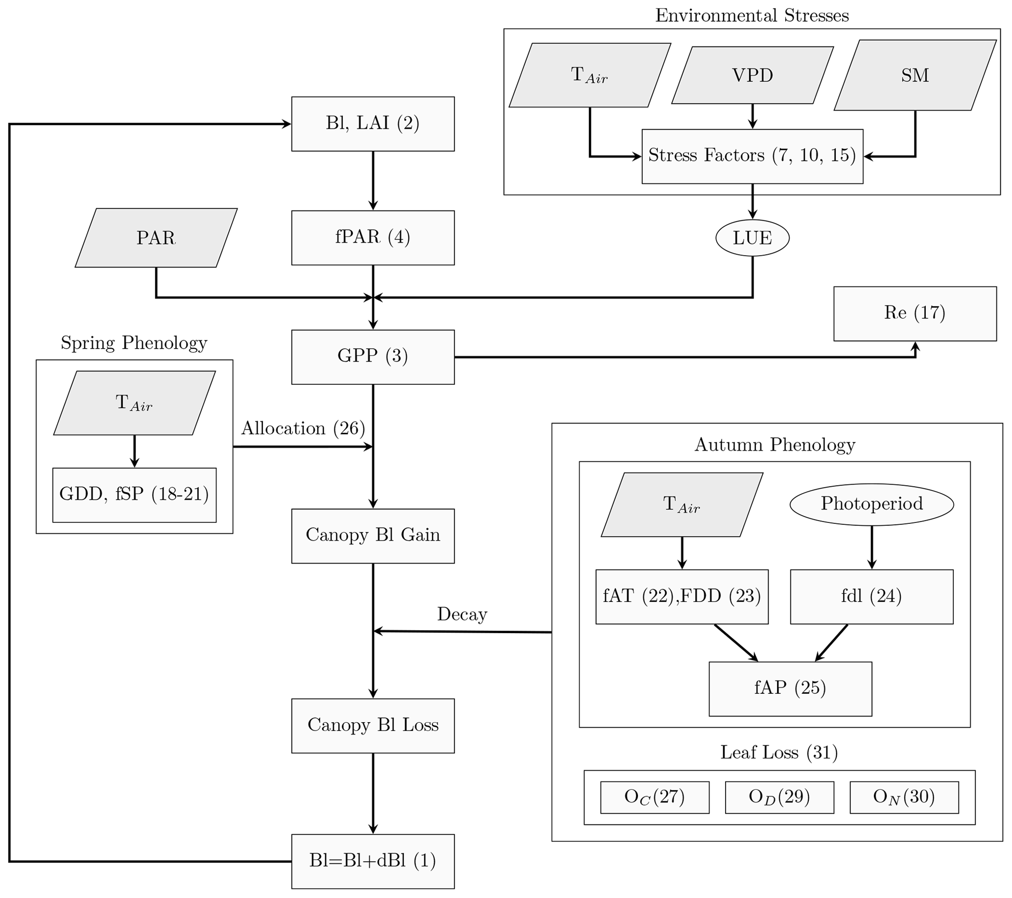
Figure 1Schematic representation of the PCM model. The parallelograms indicate the model inputs; TAir: air temperature; VPD: vapor pressure deficit; SM: soil moisture; and PAR: photosynthetically active radiation. Rectangles are the processes in the model. Variables in ellipses show LUE and photoperiod. Numbers refer to the corresponding equations in the text.
PCM uses a daily time step, during which it simulates the processes of carbon uptake, leaf respiration, carbon allocation, and carbon decay from the leaf pool (canopy) using a mass balance equation (Istanbulluoglu et al., 2012; Yue and Unger, 2015; Pasquato et al., 2015; Melton and Arora, 2016; Ruiz-Perez et al., 2017). The main governing equation to simulate the daily development of GPP(t) and Bl(t) is
where Bl(t) is leaf biomass, GPP(t) is gross primary productivity, Re(t) is leaf respiration, λ(t) is the carbon allocation coefficient, and D(t) is leaf decay components at day t. All terms on the right-hand side are calculated in the modules of the PCM. The LAI (related to Bl(t) in Eq. 1) is defined as
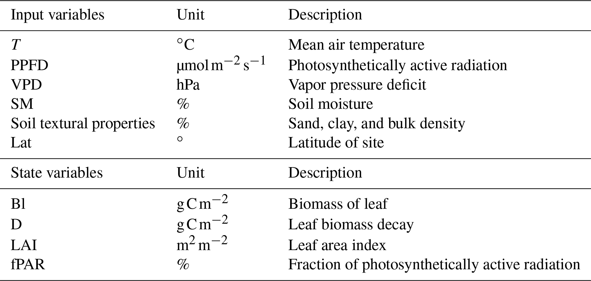
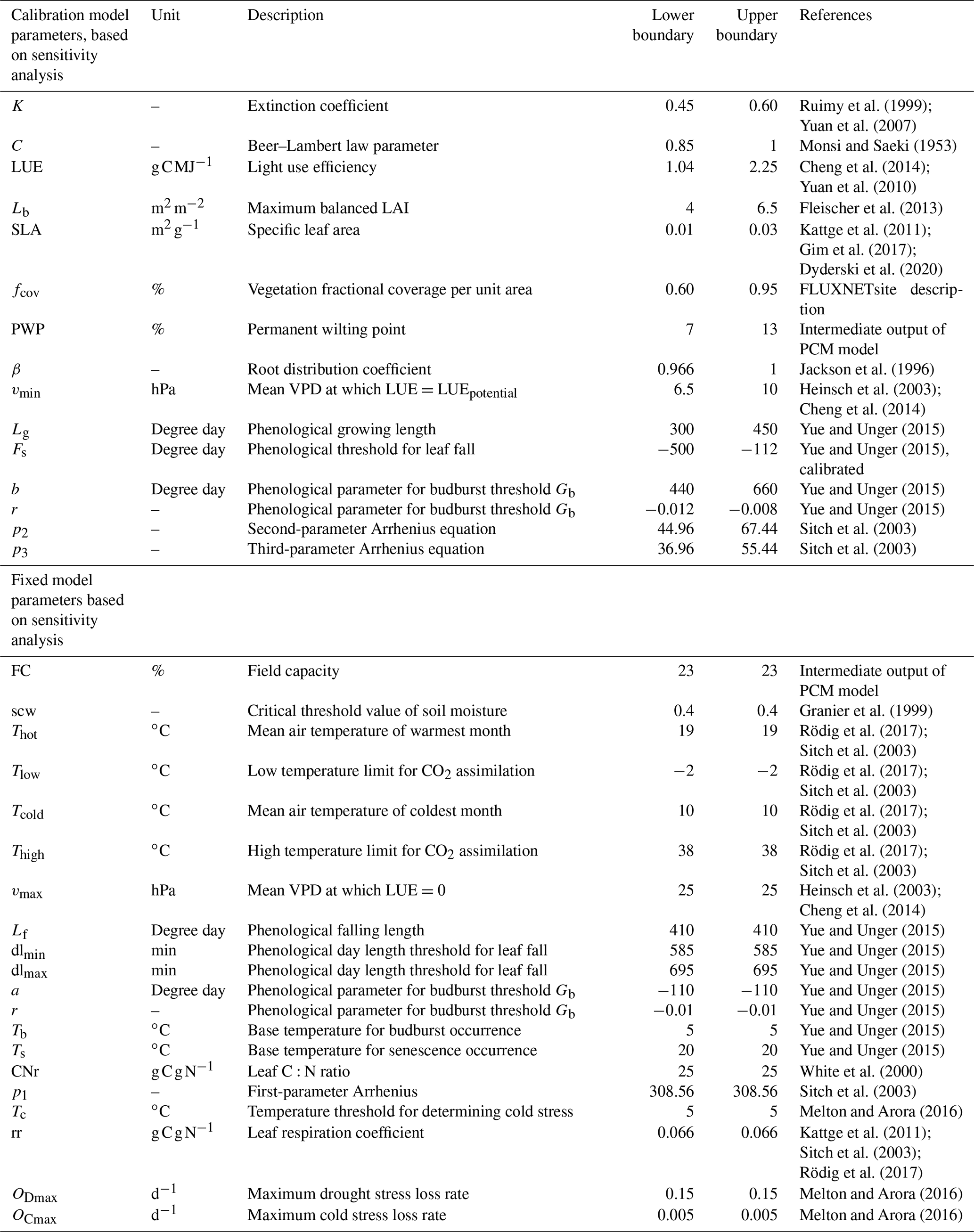
where SLA is the specific leaf area index, and fcov is the vegetation fractional coverage. In the following sections, the modeling approaches implemented for each submodel component are described in detail. A summary of the model inputs and underlying parameters is provided in Tables 2 and 3, respectively.
2.1.1 Gross primary productivity
The theoretical soundness and practical convenience of the LUE concept in estimating terrestrial GPP has been the main core of several model developments (Monteith, 1972; Wei et al., 2017; Running et al., 2000; Arora, 2002; Schaefer et al., 2012; Zhang et al., 2015) at the regional and global scales (Potter et al., 1993; Yuan et al., 2007; Xiao et al., 2004; Running et al., 2000). In this study, we likewise utilize the LUE approach, which theoretically relies on the concept of the interception of photosynthetically active radiation by plant leaves and the conversion of the intercepted radiation into biomass through the energy-to-biomass efficiency factor (i.e., LUE factor). As expressed in Eq. (1), the PCM simulation starts with the assimilation of the carbon flux (GPP) by the leaf component. The GPP flux (Eq. 3) is estimated as a product of incident photosynthetically active radiation (PAR) by means of fPAR, which is a fraction of PAR being absorbed by the plant leaf, and an LUE factor, multiplied by a modifier factor when environmental constraints are present (ϵ):
where LUE is biome-specific, unstressed (or maximum) vegetation light use efficiency parameter. fPAR is calculated as follows (Ruimy et al., 1999; Xiao et al., 2004; Yuan et al., 2007):
where c refers to the maximum absorption at full light interception in deciduous broad-leaved forest biomes (Monsi and Saeki, 1953; Ruimy et al., 1994), and k is the light extinction coefficient parameter.
ϵ (Eq. 3) is an overall, integrated modifier that corresponds to environmental stress factors. The overall modifier factor diminishes the potential value of the light use efficiency of vegetation during unfavorable environmental conditions (Potter et al., 1993). These unfavorable conditions include, for example, high and/or low temperature fT, water availability fSM, and elevated vapor pressure deficit fVPD stress factors (Zhang et al., 2015; Pasquato et al., 2015).
In general, the calculation of ϵ across different LUE models can be expressed either in minimum (Eq. 5) or multiplicative (Eq. 6) approaches to integrate different environmental stress factors. On the one hand, models such as the eddy covariance-light use efficiency model (EC-LUE; Yuan et al., 2007) uses Liebig's law of minimum stress, which emphasizes the most limiting resource to constrain GPP (Eq. 5). On the other hand, models such as the Carnegie–Ames–Stanford approach (CASA; Potter et al., 1993) and the vegetation photosynthesis model (VPM; Xiao et al., 2004) follow a multiplicative approach of stresses (Eq. 6). In the present study, we opt for the first approach in order to integrate different stress factors and to calculate the ϵ.
The first approach (minimum) is expressed as follows (Running et al., 2000; Sitch et al., 2003; Prince and Goward, 1995):
The second approach can be written in a multiplicative way:
The individual stress factors are dimensionless scalars ranging between 0 (full stress) and 1 (no stress) and are introduced in more detail in the following section.
2.1.2 Environmental constrains and GPP
(I) Temperature stress factor (fT). The first reduction factor of GPP, fT, which is related to air temperature, is calculated by including two factors corresponding to low temperature ρl (cold) and high temperature ρh (heat) stress effects (Eqs. 7–9) (Sitch et al., 2003; Fischer et al., 2016; Rödig et al., 2017):
The stress induced by the cold stress factor (ρl(t)) can be calculated as
where
The heat stress factor is calculated as
where T(t) is the daily mean air temperature; Tlow and Thigh are DBF biome-specific parameters representing high and low temperature limits for CO2 assimilation, respectively. Thot and Tcold are the monthly mean air temperatures of the warmest and coldest months, respectively, that a DBF biome can cope with (Boons-Prins, 2010; Bohn et al., 2014; Fischer et al., 2016; Rödig et al., 2017).
(II) Vapor pressure deficit stress factor (fVPD). The canopy's photosynthesis rate is strongly related to changes in vapor pressure deficit (VPD) (Konings et al., 2017; Xin et al., 2019), as photosynthesis declines due to stomata closure (Yuan et al., 2019) when atmospheric VPD increases. It can be modeled as follows in Eq. (10) (Jolly et al., 2005):
where VPD(t) is the daily vapor pressure deficit; vmin and vmax denote lower and upper thresholds for photosynthetic activities, respectively. The fVPD value of 1 indicates no stress on GPP, whereas there is full stress when the fVPD becomes 0; values between 0 and 1 result in partial and linear reduction on the GPP.
(III) Soil moisture stress factor (fSM). In general, the impact of the soil water deficit on photosynthesis in vegetation models is represented as a generic soil moisture stress function using either modeled or field observations of soil moisture content (Cox et al., 1999; Granier et al., 2000; Fischer et al., 2016). Here, we use field observations from different vertical soil profiles, including volumetric soil moisture content and soil textural properties (wherever available), to calculate the soil moisture stress factor (fSM).
Essentially, the influence of soil moisture on plant productivity depends not only on the soil moisture over the entire profile but also on the available soil water to the plant roots. Therefore, to estimate the availability of water to plants, the characteristics of the root system, including rooting depths and its distribution at different soil depths, are essential factors to be considered (Ostle et al., 2009). Thus, we include plant rooting distribution in our analysis, following Jackson et al. (1996), to take into account the root fraction at different soil depths, and weigh the soil moisture content layer-wise according to the present fraction of roots in that layer. In doing so, we calculated the cumulative root fraction (Rci) from the surface to a certain depth (d) in the soil profile for each layer (i) using the biome-specific parameter, β, as follows (Eq. 11) (Jackson et al., 1996):
Then, to estimate the root fraction in each individual layer (Rii; Eq. 12), we use the calculated cumulative root fraction of each layer subtracted from the corresponding fraction of the previous layer (see Eq. 11). Next, Rii is multiplied with the corresponding observed soil moisture content of that layer to calculate the soil moisture contribution from each layer individually (Eq. 13). Later, by summing up the soil moisture contributions from all individual layers (θi), a daily effective soil moisture content, θ(t), over the soil column is obtained (Eqs. 12–14).
Similar to other stress terms, the soil moisture stress factor varies between 0 and 1 and is quantified as follows (Eq. 15):
where θ(t) is the daily effective soil moisture; θr and θMSW are water storage corresponding to the permanent wilting point and the critical point below which transpiration is limited, respectively. θMSW, representing minimum soil water content for unstressed photosynthesis (Hartge, 1980; Granier et al., 1999; Fischer et al., 2014), is calculated as follows:
where θs is soil water content at field capacity; scw (soil critical water content) is a constant threshold commonly set at 0.4 and a calibration parameter in PCM – scw is a physiological threshold defined as the critical relative soil water content at which tree transpiration begins to decrease (Granier et al., 1999). According to Granier et al. (1999) and Fischer et al. (2016), the scw value does not vary significantly between soil and plant species and can be considered as a constant value. The θr and θs correspond to soil matric potentials of −1.5 and −0.033 MPa, respectively.
When the daily effective soil moisture content is above a minimum soil water content (θMSW; Eq. 16), there is no stress to limit photosynthesis, while below the θMSW point, there is a linear increase in stress as water content decreases until θr is reached. At this point, the soil water stress factor becomes 0 with full limitation on photosynthesis and GPP (Harper et al., 2021).
2.1.3 Canopy respiration
To allow the estimation of daily changes in carbon in the leaf pool (Eq. 1), the release of carbon to the atmosphere from leaf respiration (Re) has to be calculated. This flux is part of gained carbon (i.e., GPP) consumed for self-maintenance requirements in the leaf pool. In fact, the canopy's net primary productivity (NPPcanopy), which is the net available carbon ready to be allocated among different plant pools, is the sum of photosynthetical carbon uptake by plants (GPP) reduced by carbon loss via leaf respiration (Re) (Pasquato et al., 2015; Running et al., 2000; Melton and Arora, 2016).
We use the well-established modified Arrhenius equation (Eq. 17) (Lloyd and Taylor, 1994; Sitch et al., 2003; Perez, 2016) to calculate the leaf respiration. The Re flux is a function of air temperature, the carbon mass of the leaf pool, and a tissue-specific carbon to nitrogen ratio, given as
where rr represents the leaf respiration rate and Bl the carbon mass of leaf pool (leaf biomass); p1, p2, p3 are parameters in the Arrhenius equation, CNr is the carbon to nitrogen ratio in leaves, and T is daily mean air temperature.
2.1.4 Vegetation phenology module
We incorporated a phenology submodel into our model using the approach defined in Yue and Unger (2015). This submodel calculates temperature-dependent phenological factors for spring and autumn – fST and fAT, respectively. These factors range from 0 to 1 throughout the year to determine the timing of the spring budburst (once the spring temperature-dependent factor increases to be above 0), maturity (when the spring temperature-dependent factor approaches 1), autumn senescence (once the product of the autumn temperature-dependent and photo-period factors start to decrease below 1), and dormancy (once the product of autumn temperature-dependent and photo-period factors approach 0) phenophases. The second phenological factor in the autumn and dormancy phenology is the photo-period (fdl) factor, which depends on day length. The photo-period factor, together with the temperature-dependent factor, regulates the leaf senescence. The phenology submodel determines the above-mentioned four phenological transition dates on which a simple allocation of assimilated carbon to the leaf pool is based. Below, we provide details of each phenological factor and event.
(I) Spring phenology (fSP). The growing season starts with the budburst day, which is the beginning of canopy development and the time when green tips of leaf begin to show. It is estimated using a temperature-dependent phenological factor, fST, as follows (Eq. 18):
where GDD is the growing degree day and Gb is the budburst threshold value. The Lg parameter is a calibrated constraint in degree day, representing the period of leaf growth from budburst to maximum leaf cover (Yue and Unger, 2015). The accumulation of growing degree day (GDD) (Eq. 19) from winter solstice day is calculated as follows:
where T10 is 10 d average air temperature. Tb is the base temperature for the budburst (5 ∘C). In the estimation of fST (Eq. 18), Gb is a threshold value for budburst to occur and is calculated as follows:
where a, b, and r are parameters for the budburst threshold. NCD is counted as the number of chill days between the previous winter solstice day and the beginning of the successive year. Given the GDD and Gb estimates, the temperature-dependent phenological factor (fST) is then applied to calculate the spring phenology (fSP) (Eq. 21):
(II) Autumn phenology (fAP). For the autumn phenology, the product of two phenological factors – temperature fAT and photo-period fdl factors – is considered to estimate the timing of senescence and dormancy. The autumn temperature-dependent factor, fAT (Eq. 22), is obtained as follows:
where Fs is a threshold in degree day for leaf fall, and Lf is a threshold in degree day for the duration and length of the leaf falling period (more details can be found in Yue and Unger, 2015). FDD (Eq. 23) is an accumulative falling degree day from summer solstice day and is known as a cumulative cold summation method (Yue and Unger, 2015); it can be calculated as
where T10 d is 10 d average air temperature; Ts is base temperature for leaf fall at 20 ∘C.
In addition to the temperature factor fAT, autumn senescence timing is regulated via the photo-period factor fdl, which is calculated based on day length (dl) period together with the lower (dlmin) and upper (dlmax) limits of day length affecting leaf fall, as in Eq. (24):
where dl is the day length in min; dlmin and dlmax are the lower and upper limits of day length for the period of leaf fall, respectively. The autumn phenology (fAP) is finally calculated as a product of fAT and fdl (Eq. 25):
The predicted phenological transition dates from the spring fSP and autumn fAP phenology factors determine the budburst-maturity and senescence-dormancy events, respectively. Based on this information, a fractional allocation to and decay from the leaf pool is considered (as detailed below).
2.1.5 Carbon allocation to and decay from the leaf pool
The next step of the carbon pathway in Eq. (1) is the allocation to and decay of assimilated carbon from the leaf pool. The leaf biomass state variable (Bl) in Eq. (1) is updated at a daily time step, based on changes in the gain and loss of carbon in the leaf pool. The allocation and decay processes are both key physiological processes in the vegetation models, governing the partitioning of growth among different plant carbon pools, and are critical determinants of plant productivity (Haverd et al., 2016; Xia et al., 2017). In vegetation models, there are two widely used allocation schemes, which are based on: (1) fixed allocation coefficients, and (2) allocation driven by allometric constraints. The first scheme uses a fixed allocation ratio for individual plants' carbon pools (e.g., used in CASA, Friedlingstein et al., 1999, or BIOME-BGC, Hidy et al., 2022). In this scheme, the allocation ratio is constant within different plant development stages. In the second scheme, a fraction of carbon is allocated in such a way that it satisfies allometric relationships that exist between various plant compartments (Malhi et al., 2011; Gim et al., 2017). In the case of allocation to the leaf, the allometric relationship is based on the relative mass of the canopy – the so-called maximum Lb – that a plant can support with a certain stem mass and height. We adopted an allocation scheme that mainly depends on an updated daily carbon status of the leaf pool. We use the maximum values of balanced LAI supported by the system (Eq. 26) based on a previous study conducted by Fleischer et al. (2013). Instead of considering it as a fixed value, we vary Lb within a range of ±1 m2 m−2 and consider it as one of the model parameters.
where λ(t) is the carbon allocation ratio to the leaf pool, and Lb is the maximum LAI that can be supported by plants.
Provided with the identified major phenological transition dates from the phenology submodel – i.e., budburst, maturity or steady growth, senescence, and dormancy – the calendar year is accordingly divided into four main stages. During the early growing season, once the climate condition becomes favorable for plant growth and the budburst occurs, carbon allocation to the leaf, λ (Eq. 26), is a relatively large fraction. This means that the largest part of the carbon will be partitioned towards the leaf and will be used for growth during the early growing season (Gim et al., 2017). Given the value for balanced LAI supported by the system (Fleischer et al., 2013), the carbon allocation slowly decreases with an increase in LAI until the leaf mass reaches that balanced LAI. As soon as the canopy approaches a full-leaf state (i.e., maturity phenophase), the carbon allocation ratio to the leaf is held at its minimum – a small portion is used for maintenance respiration during this steady growth stage. We set the leaf allocation ratio during the maturity phase to a value of 5 % from the assimilated carbon, following the recent version of the Noah-MP model's leaf allocation scheme (Gim et al., 2017).
After the steady growth and maturity phase, the leaf senescence phase approaches and the leaf-loss processes start to play the main role in moderating the mass balance of the canopy and the corresponding LAI seasonality. The loss of carbon via the leaf fall in PCM is simulated based on the calculated senescence and dormancy transition dates via the phenology submodel, such that when the simulation time-step approaches the senescence date, the model linearly decreases the leaf biomass until the leaf biomass nearly reaches 0 at the beginning of the dormancy phase.
Concerning the leaf loss processes, PCM also accounts for leaf losses due to cold stress (OC) (Eq. 27), drought stress (OD) (Eq. 29), and normal loss of the leaf (ON) (Eq. 30) following the schemes of the CLASSIC model (Melton and Arora, 2016).
Leaf loss due to the cold stress is given by
where OCmax is the maximum leaf loss rate parameter, and Cs is a cold stress factor value. The cold stress factor (Eq. 28), ranging between 1 (full stress) and 0 (no stress), is calculated as
where T(t) is air temperature, and Tc is a biome-specific temperature threshold below which leaf damage is expected.
Similar to the OC, the leaf loss rates due to drought stress OD (Eq. 29) are calculated using the fSM stress factor (through the soil moisture stress submodel) and a OCmax maximum leaf loss rate parameter associated with the drought stress:
The third leaf loss term represents the loss rates due to a normal decay ON, driven by biome-specific leaf lifespan (τ=1 for DBF in Eq. 30), given by:
Finally, the total decay of leaves D(t) consists of contributions from all individual losses (Melton and Arora, 2016) and can be given as follows (Eq. 31):
where OC, OD, and ON are the leaf loss rates due to cold stress, drought stress, and normal decay, respectively.
In summary, the proposed PCM model comprises the submodels mentioned above in a hierarchical chain, starting with the carbon uptake via the initial leaf biomass state variable and continuing with the daily partitioning of the assimilated carbon together with daily decay from the leaf compartment to calculate the leaf biomass production increment. This biomass increment is later added up to the state variable from the previous time step to update the leaf biomass for the current time step. Finally, to update the LAI that is required for the GPP estimation over the next time step, the current leaf biomass is converted to LAI according to Eq. (2).
2.2 Model setup and experimental design
2.2.1 Study sites and datasets
This study focuses on deciduous broad-leaved forest biome types. We selected tower sites distributed over Europe and North America to ensure a representative spatial coverage. Sites were excluded if data for fewer than 5 consecutive years of observations were available. We further screened the data at each site to only include the years with minimal gaps in the input data. For example, there were some long periods (i.e., years) of gaps within the continuously recorded FLUXNET dataset for photosynthetic photon flux density (PPFD); we excluded those years in the simulations (e.g., a continuous period of missing PPFD in the US-Ha1 dataset from 1991–2003). Applying the above criteria, nine sites with varying temporal coverage were retained for the analyses (Fig. 2). The general site information is presented in Table 1. Daily flux and meteorological forcing data are from ecosystem stations available from the free, fair-use FLUXNET2015 Tier 1 global collection database (https://fluxnet.org/data/download-data/, last access: June 2021) (Pastorello et al., 2020). The input data required to drive the PCM comprise air temperature (T), photosynthetic active radiation (PAR) (i.e., converted from PPFD in ), and vapor pressure deficit (VPD) (Table 2). The tower-based GPP estimations – GPP_NT_VUT_REF from the FLUXNET2015 dataset – are used for model calibration. We used the first year of the time series as a warm-up period, during which the chilling days and thermal requirements in the phenology submodel are counted. In other words, since the phenology module for each individual year needs the number of chilling days from the previous year, the very first year of observations is not included in the simulations. The very first year of observations is only used to calculate budburst day of the first simulation year. Here, the warm-up period refers to the last 10 to 11 d of each previous year that are eventually required for estimating variables in the phenology module for its uninterrupted run in the subsequent year. When simulating the soil moisture stress in establishing the model is desired, soil moisture (SM) and soil textural properties are also included. We investigate the impact of soil moisture stress at the Hohes Holz (DE-HoH) site in Germany only, where soil moisture data are available up to 80 cm depth. With regard to calculating the soil moisture stress in PCM, a pedotransfer function following Zacharias and Wessolek (2007) is implemented to estimate site-specific θs and θr values. This (pedotransfer) submodel receives soil textural properties (sand, clay contents, and bulk density) obtained from field observations of spatially distributed soil profiles as input. It provides the required field capacity (θs) and permanent wilting point (θr) to calculate θMSW and the corresponding soil moisture stress term fSM in the calculation of ϵ (Eq. 5). To maintain the consistency with the vertically weighted soil moisture, θs and θr are estimated as weighted average values of individual, layer-specific θs and θr, taking the respective root fractions as a weighting factor. Other required parameters in the model related to different processes are listed in Table 3. The LAI field measurements were obtained via personal communication with site contact persons, and a subset of 4 sites (DE-HoH, DE-Hai, US-MMS, and US-Ha1; https://harvardforest1.fas.harvard.edu/exist/apps/datasets/showData.html?id=hf069, last access: 5 January 2022) was selected based on data availability to evaluate the modeled LAI. The observation-based LAI data were obtained using common procedures – either the LAI-2000 instrument (Gower and Norman, 1991) at the DE-Hai, US-MMS, and US-Ha1 or the fisheye (DHP) technique (Bonhomme and Chartier, 1972; Ariza-Carricondo et al., 2019) at the DE-HoH site. These two methods agree very well according to Ariza-Carricondo et al. (2019) and are thus considered to yield comparable values across different sites (Ariza-Carricondo et al., 2019).
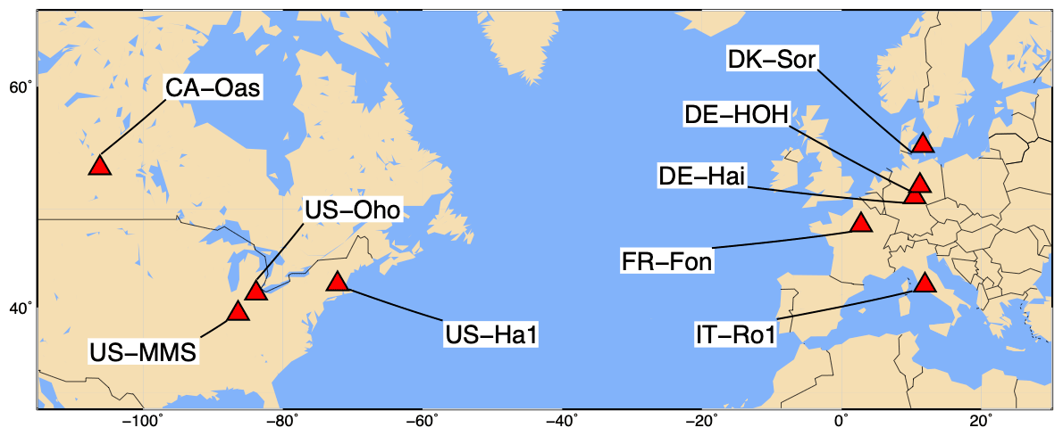
Figure 2Location of the FLUXNET2015 sites investigated in this study.
Table 1Descriptions of flux tower sites from FLUXNET2015 global database collection. Note that, since the phenology submodel for simulating budburst in each year needs the temperature data from the last 10–11 days of the previous year, the very first year of the investigation period at each site is not included in the simulations.
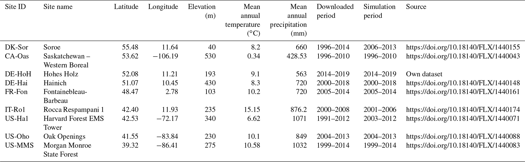
Table 2List of input and state variables (at daily time step) in PCM.
2.2.2 Model structure and setup
The impact of water availability (i.e., soil water deficits and atmospheric water deficits) on canopy photosynthesis in vegetation models is structured in two ways: individually or in combination with each other. Recently, plant hydraulic theory has also been introduced to reflect the vegetation water stress in the Community Land Model (CLM5), which is beyond the scope of this study (Kennedy et al., 2019). In some models, water stress is quantified as an overall stress from both atmosphere and soil (GLO-PEM; Prince and Goward, 1995, BIOME-BGC; Hidy et al., 2022). For instance, in the GLO-PEM model, the water stress condition is reflected by an estimated and potential evapotranspiration, a relative drying rate scalar for potential water extraction, and a volumetric soil moisture content (more details, together with equations, can be found in Zhang et al., 2015). Some other models account for the water stress only due to the atmospheric drought (CASA; Potter et al., 1993, MOD17 algorithm; Running et al., 2000). For example, in the MOD17 algorithm, only the atmospheric variable VPD and its two parameters, vmin and vmax, are used to calculate the water stress factor to predict GPP (Running et al., 2000). In some other models, such as FORMIND (Fischer et al., 2016) and EC-LUE (Yuan et al., 2007), only the soil moisture deficit is reflected. For instance, in the FORMIND model, the impact of the atmospheric water deficit (VPD impact) is not presented; however, the soil moisture deficit is represented by volumetric soil water content and soil parameters (soil field capacity, permanent wilting point, and minimum soil water content). In order to determine how stress should be represented in the final version of PCM, we conducted two sets of preliminary model experiments to examine (1) whether the inclusion of fSM in addition to the other stress factors affects the results, and (2) the effect of alternative integration approaches (i.e., Liebig's law and multiplicative approaches, see Sect. 2.1.1) on simulated GPP over the DE-HoH site during the drought in 2018. Since the best model skill of the PCM was achieved when incorporating all stress factors (fT, fVPD, and fSM) in the calculation of the overall environmental stress and when using the minimum integration approach (Eq. 6), this structure was selected for the final setup (see Figs. S1 and S2 in the Supplement). With regard to specific considerations in LAI simulations, the model starts with the simulation using a fixed initial LAI state variable to begin the carbon assimilation once weather conditions become more favorable for plant growth. Following the CABLE model parameterizations (Li et al., 2018), we set the initial LAI value to 0.35. We also consider a local maximum LAI (so-called Lb in this study), obtained from reported values in the literature (Fleischer et al., 2013), that individual mature forests can sustain at canopy closure. However, the local maximum LAI is, later in the calibration step, allowed to vary within ±1 m2 m−2 of the reported value. The Lb constrains the simulated LAI up to the reported value at each site across years.
2.2.3 Global sensitivity analysis
Despite the simplicity of parsimonious models, assessing model robustness remains a fundamental step when building and developing a model. One of the powerful and invaluable tools for robustness assessment is global sensitivity analysis (GSA) to test the underlying model parameterizations and to reveal sensitive model parameters for the subsequent parameter inference. In general, the GSA can be performed to understand the influence of parameter perturbations on modeled simulations and to determine the informative parameters that contribute the most to an output behavior (Iooss and Lemaître, 2014; Cuntz et al., 2016; Rakovec et al., 2014). In this study, during the GSA, the parameters vary over boundaries reported in the literature. In case there were no reports of upper and lower bounds available for some parameters (e.g., phenological parameters from Yue and Unger, 2015), we varied them at ±20 % level of their default values. We utilize the Sobol' variance-based sensitivity method (Saltelli et al., 1999) with the Sobol2002 formula (Saltelli, 2002), in which decomposition of the output variance is performed in terms of Sobol' indices. The Sobol' first-order index (Si) and total-order Sobol' index (ST) express the share of output variance associated with a given parameter i and the share of output variance where all parameters are varied except the parameter i, respectively. These indices range between 0 and 1, with 0 value indicating that the model output is entirely insensitive to the respective parameter changes. The closer the value is to 1, the more important and sensitive the respective parameter. Generally, the model parameters are deemed sensitive if the sensitivity index is above a certain threshold value. Here in this study, we report the total-order Sobol' index and set the selection threshold at 1 % (Tang et al., 2007), meaning that if the variation of a given parameter contributes to a change greater than 1 %, then that parameter is recognized as an informative parameter. In contrast, non-informative parameters are reported as parameters with Sobol' indices below 1 %. Given the focus of the present study on two main output variables (i.e., GPP and LAI), we use the time mean for both outputs over the entire period for the sensitivity analysis at each study site. However, the results are expected to differ not only according to the site and selected target output but also between the individual years if a specific year is of investigative interest (Göhler et al., 2013; Hou et al., 2012). To conduct the sensitivity analysis, we opt to use all coefficients in the empirical equations as adjustable parameters (Table 3). It helps to explore the model sensitivities of often hidden parameters to properly constrain the model (Cuntz et al., 2016). Overall, we apply the global sensitivity analysis to all study sites for the common 29 parameters and analyze the sensitivity of the soil moisture stress parameters together with other parameters only for the DE-HoH site at which representative soil moisture data at different depths, down to 80 cm into the soil, were available. Given the importance of the number of model evaluations required to conduct the Sobol' sensitivity analysis (Nossent and Bauwens, 2012) and the stability of sensitivity indices, we also check the convergence of the Sobol' indices through a visual assessment of diagnostic plots.
2.2.4 Parameter estimation
Based on the results of the sensitivity analysis, informative and non-informative parameters were identified. Later, we fixed the non-informative parameters to their corresponding values reported in the literature (see Table 3 for details); the remaining informative parameters were inferred using a Monte Carlo approach (Kuczera and Parent, 1998). The parameters were calibrated against the GPP_NT_VUT_REF time series from the corresponding flux tower measurements (global FLUXNET Tier1 network, accessed on 13 February 2021) (Pastorello et al., 2020). It is important to note that, besides the maximum LAI value, we did not use LAI field observations in the calibration process, as LAI is not readily available from the FLUXNET dataset. Instead, some LAI observations (obtained from site contacts) were used in the model validation step. The first year of the dataset is considered a spin-up period. The rest of the time series are divided into two sub-periods. The first half is used for the calibration phase, and the remaining years are used to independently evaluate the model performance (i.e., over the out-of-calibration set). A total of 10 000 parameter sets were sampled from their a priori defined ranges (Table 3) in each study site to estimate the parameters and to simulate the GPP flux and LAI. Model performance was quantified using a group of performance metrics, including Kling–Gupta efficiency (KGE) (Gupta et al., 2009), root-mean-square error (RMSE), and coefficient of determination (r2). We selected an ensemble of informative model runs that simultaneously lie within the top 5 % of all the performance metrics.
2.2.5 Site-specific validation and model generalization
The second half of the GPP time series at each study site was used for the model validation step. In addition to the at-site validation, it is also equally important to consider the generality of the model structure, including underlying model parameterizations. To this end, we considered an independent (spatial) validation approach – so called cross-validation – for assessing the robustness of model parameterizations beyond the conditions during which they were calibrated. The relevance of the cross-validation to the modeling framework is that transferable models can be used beyond the spatial and temporal limits of their underlying data, especially in the face of the pervasive scarcity of observational data to constrain model parameterizations (Yates et al., 2018). Therefore, as the next step in our modeling framework, after performing the site-specific calibration and validation, a cross-validation of the model is conducted to come up with a compromise solution (here, the parameter set) applicable across the study sites, following the approach of Zink et al. (2017). In doing so, the behavioral parameter sets found from the on-site calibration for each study site are grouped together as one unique set of all possible behavioral parameters. Then the model is run using all possible parameter sets, and the respective performance metric (i.e., KGE) for each parameter set at each investigated site is estimated. After that, the mean values of KGEs corresponding to each parameter set over all the study sites are calculated. Finally, a set of parameters associated with the highest mean KGE score is recognized as a compromise solution. Here, the goal of this analysis is to investigate the generality of the underlying model structure and to allow the inference of a common (compromise) set of model parameters for the PCM for a broader applicability (i.e., beyond the calibration sites).
In the following section, we first show and discuss findings from the global sensitivity analysis and site-specific parameter calibration. This is followed by a discussion of the site-specific model performance. Finally, we present the results of a cross-validation to test the generality of underlying model parameterizations. This also allows us to propose a standard set of PCM parameters for locations where calibration is not possible.
3.1 Sensitivity analysis
Here, we explore the sensitivity of the output variables (i.e., GPP and LAI) to the model parameter variations using Sobol' method at each study site. Although a direct comparison of PCM parameters sensitivities from this study with similar models in other studies is difficult due to differences in model structures and representation of photosynthesis processes, one can gain insights by comparative assessments among conducted studies. For instance, the light utilization in LUE-oriented GPP models is based on photon absorption and photosynthetic efficiency of incident light (Frost-Christensen and Sand-Jensen, 1992). Hence, one can compare the significance of the LUE parameter of our model with that of the quantum yield of photosynthesis, which is a measure of photosynthetic efficiency in the Farquhar equation (Farquhar et al., 1980) in several land surface models. As can be seen from Fig. 3a (mean GPP) and b (mean LAI), different sensitive parameters are associated with different output variables. However, for the same output variable, all sites more or less share a similar informative set of parameters, although the magnitudes differ. Furthermore, the evaluation of Sobol' indices convergence (see Fig. 4) showed relative stability of sensitivity indices at around 8000 model evaluations. In the following, we show and discuss the sensitivity of the model outputs to different PCM parameters.
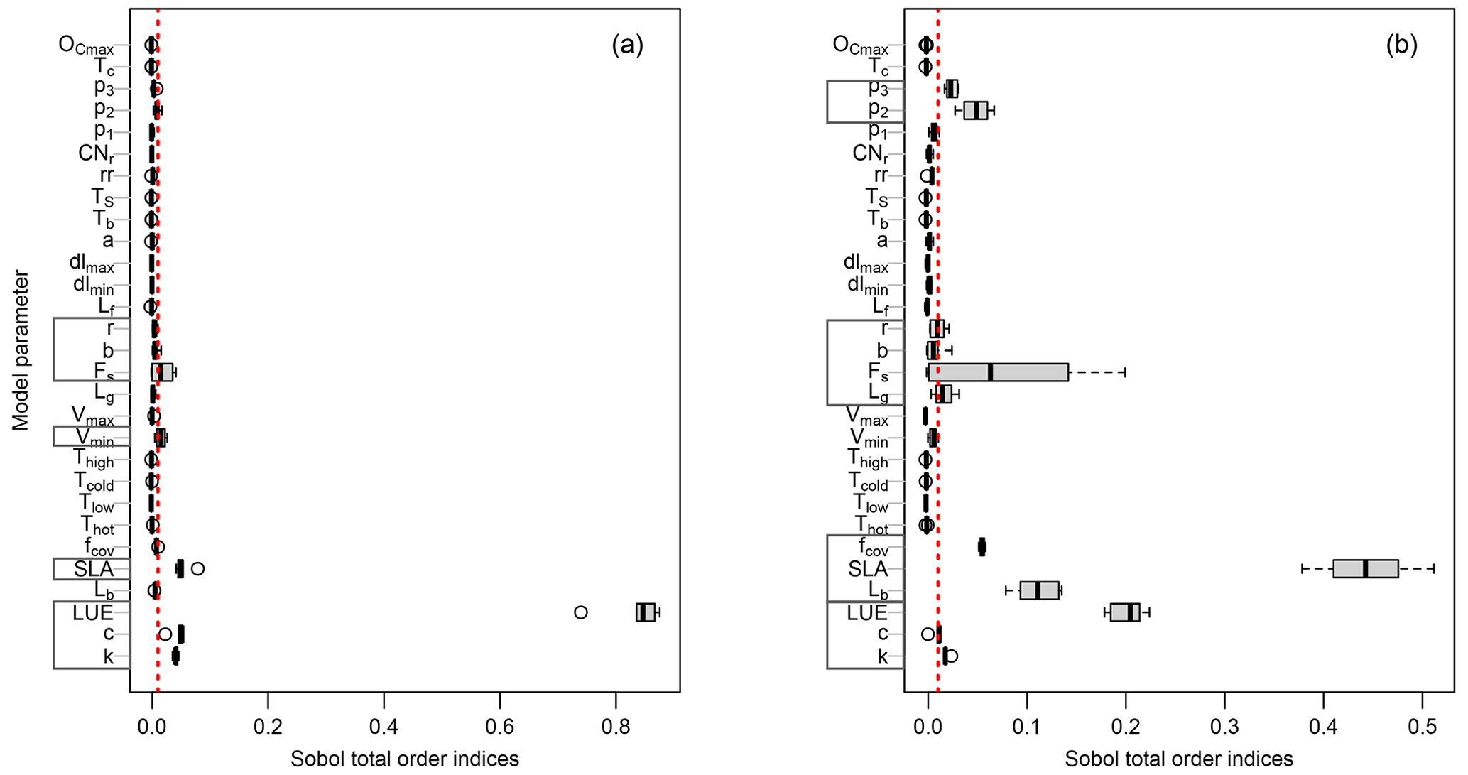
Figure 3Distribution of the total-order Sobol' indices for GPP (a) and LAI (b) outputs across all sites. Each gray box on the y axis represents parameters involved in a specific process as follows: GPP-related parameters (Eqs. 3 and 4); LAI-related parameters (Eqs. 2 and 26); environmental stresses-related parameters (Eq. 10); phenology-related parameters (Eqs. 18, 20, and 22); canopy respiration-related parameters (Eq. 17). The vertical dotted red line corresponds to the threshold of 1 %.
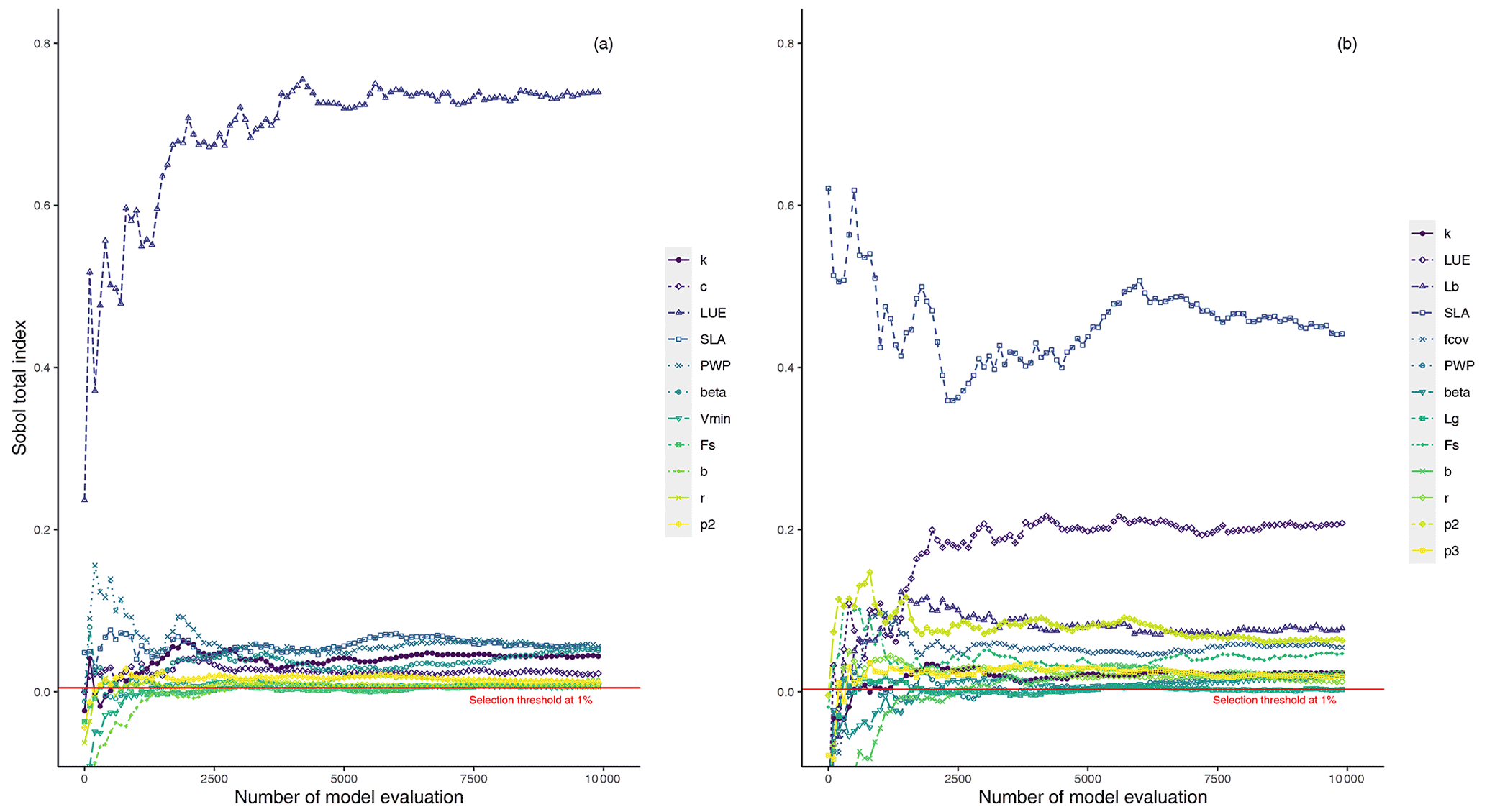
Figure 4Illustration of the evolution of total-order Sobol' indices (total-order indices convergence) for sensitive parameters with an increasing number of samples for GPP (a) and LAI (b) outputs at the DE-HoH site, taken as an example including soil moisture stress-related parameters.
3.1.1 Parameter sensitivity for GPP estimation
We first investigate the sensitivity of GPP output to the model parameters. Figure 3a shows the total-order Sobol' index of all parameters contributing to the GPP output. The boxes in Fig. 3a indicate the variation of the sensitivity of a given parameter across different sites. Only a small number of them out of the 34 model parameters (Fig. 3a) have ultimate control over the simulated GPP. This is in agreement with previous studies using LPJ-DGVM (Zaehle et al., 2005), BETHY (White et al., 2000), and BIOME-BGC (Knorr, 2000) models showing only a few of the investigated parameters significantly influencing the modeled carbon flux outputs (including GPP).
The most sensitive parameter for the GPP estimates turned out to be the light use efficiency (LUE) in Eq. (3). This agrees with numerous other studies confirming that light use efficiency is a significant parameter affecting GPP. For instance, Zaehle et al. (2005) conducted a probability-based sensitivity analysis using the LPJ-DGVM ecosystem model, utilizing the Farquhar photosynthesis scheme, and found that carbon fluxes (including GPP) are highly sensitive to parameters related to the photosynthesis process, particularly the intrinsic quantum efficiency parameter (so called αq in their model), which is related to the LUE in PCM. Similarly, Ma et al. (2020), using a GSA in the Flux-based ecosystem model and based on the Farquhar photosynthesis scheme, found canopy quantum efficiency of photon conversion to be among the most sensitive parameters with a strong influence on forest GPP. The multiplicative coefficient of canopy reflectance, C, and the light extinction coefficient, k, parameters in the fPAR formulation (Eq. 4) based on Lambert–Beer's law also showed substantial sensitivities. Notably, these parameters are fixed to constant values by default in the fPAR formulation in similar studies (e.g., Xiao et al., 2004, and Xin et al., 2019), whereas, here, we let these parameters (C and k) vary at ±20 % level of their fixed values. The next group of sensitive parameters are those involved in the imposed environmental stresses on GPP. (I) The vmin parameter (Eq. 10) exhibits some sensitivity and controls the impact of vapor pressure deficit stress on simulated GPP (fVPD). Balzarolo et al. (2019) also reported the strong impact of VPD in general on radiation use efficiency and on resultant GPP. (II) The next environmental factor constraining the GPP is soil moisture stress. Here, we identify β (Eq. 11) and θr (Eq. 15) as sensitive parameters. We can only consider and discuss the soil moisture stress-related parameters at the DE-HoH site due to the lack of soil moisture data at other sites. The investigated sensitivity of fSM-related parameters are shown in Fig. S3 in the Supplement. Similar findings of the pronounced impact of parameters controlling soil moisture availability (e.g., θr and β) on simulated GPP have been reported by Li et al. (2016) for the CABLE and JULES models. From a soil science perspective, θr is often a fixed value of soil water content corresponding to a soil matric potential of 1500 kPa (Zhang and Han, 2019) and is typically not considered as a parameter. However, our result shows that θr might not be considered as fixed. Pedotransfer functions (PTFs) link soil textural properties (e.g., sand, clay contents) to soil parameters (e.g., θr), and various functional forms have been developed in past decades (Van Looy et al., 2017). Empirical coefficients of PTFs can also be regarded as model parameters (Samaniego et al., 2010; Kumar et al., 2013; Schweppe et al., 2022). Hirmas et al. (2018) also showed that soil retention properties can change over time. For example, climate change may induce rapid changes in the soil macroporosity and the associated soil hydraulic properties. Those may alter the feedback between climate and land surface.
The SLA parameter (Eq. 2), as one of the structural parameters, is also a major contributor to simulated GPP. Its sensitivity can be explained by the direct effect of SLA on the LAI calculation (Eq. 2), through which the carbon assimilation (GPP) eventually takes place (Eqs. 3 and 4). Arsenault et al. (2018) and Li et al. (2016) also reported the SLA parameter among very sensitive model parameters when simulating carbon fluxes (including GPP) in the Noah-MP and CABLE land surface models, respectively.
Finally, the last group of sensitive parameters in modeled GPP are those involved in the phenology submodel. The parameter Fs (Eq. 21), determining the timing of leaf fall, appeared as a major informative parameter for all sites; however, some parameters were only sensitive at some sites, including those for the leaf budburst threshold – namely, b and r (Eq. 19). The b parameter appeared sensitive only at DE-HoH, and the parameter r is sensitive at CA-Oas and US-Oho. Generally, the implemented phenology submodel controls the plant's active period and, at the same time, accounts for the impact of the temperature factor on leaf development and resultant GPP. This might be a reason why temperature-related parameters in the temperature stress factors (Eqs. 8 and 9) are not found to be informative in the sensitivity analysis. In other words, temperature stress limits CO2 assimilation and gross primary productivity outside of the growing season. Phenology parameters play their roles during the growing season. This period demonstrates favorable conditions for plant growth when the temperature stress is mostly not active. Therefore, temperature stress parameters do not significantly influence the modeled GPP. In agreement with our results, Yuan et al. (2007) also reported little impact by environmental stresses due to temperature on GPP during the growing season. It is worth mentioning that the temperature stress is still applied during the growing season, but as the upper-most limits of temperature ( and Thigh=38 ∘C) do not occur frequently – unless during cold or heat stresses (particularly hot years in 2018 and 2019 at the DE-HoH site) – the sensitivity of GPP to temperature parameters is less pronounced during the growing season.
Another interesting point emerging from Fig. 3a is the insensitivity of GPP output to the LAI balanced (maximum) Lb. This effect can also be seen in the LAI simulation (e.g., at DE-HoH site) where an ensemble of simulated LAI at each time step during the maturity phase (i.e., in Fig. 7) did not cause much difference in the corresponding GPP output (i.e., in Fig. 5). This is in agreement with the previous studies of Jung et al. (2007) and Lee et al. (2019), which showed that GPP output saturates and becomes insensitive at LAI values above 4 m2 m−2.

Figure 5Time series of observed and simulated GPP at each study site during the last 3 years of calibration and the first 2 years of validation. The vertical dashed line marks the calibration–validation periods. The black dots indicate the tower-estimated GPP. The light gray, shaded area corresponds to the resultant ensemble output members at each time step. The dark gray line refers to the median of ensemble members.
3.1.2 Parameter sensitivity for LAI estimation
We further explore the parameter sensitivity for LAI output similarly to the GPP described above. In general, a similar set of sensitive parameters were identified for GPP and LAI outputs across sites (Fig. 3b). However, some differences were also detected: parameters such as Lb, fcov, Lg, p2, and p3 showed substantial sensitivity, while the sensitivity to vmin was almost negligible. Regarding the similarity of parameters between GPP and LAI, it is worth noting that the calculations of GPP and LAI depend on each other, since assimilated carbon (i.e., GPP) is partly converted to leaf biomass, from which the LAI is calculated and used in turn for the GPP calculation in the next time step. Therefore, LAI output should be sensitive to roughly the same set of parameters as the GPP output. The result in Fig. 3b shows that LUE, C, and k, directly involved in the GPP formulation, have considerable influence on the LAI output. These parameters, in particular the LUE, strongly control the assimilated carbon and consequently affect the modeled LAI.
Figure 3b also shows a major contribution of SLA (Eq. 2), fcov (Eq. 2), and Lb (Eq. 24) to the LAI output. Similar to the LUE for GPP, the SLA is central for the calculation of LAI (Eq. 2) and thus shows by far the largest sensitivity. Since the LAI output in the model depends on GPP, the studies (mentioned above) that report the impact of SLA on GPP are probably applicable to LAI output as well (Li et al., 2016; Arsenault et al., 2018). The fcov parameter represents the fractional vegetation coverage per unit area and is a critical parameter in calculating forest GPP (Ma et al., 2015). Ma et al. (2015) assumed 100 % forest coverage in their calculation of GPP, from which LAI was calculated. They showed how this inappropriate assumption (i.e., 100 % forest coverage), in the place of a realistic coverage, can exaggerate the forest area when calculating forest GPP (and consequently the LAI). Here in the PCM, the fcov parameter is allowed to vary between 60 % and 95 % as an adjustable parameter (based on the Fluxnet2015 Dataset description of percent coverage greater than 60 % at DBF sites; http://sites.fluxdata.org/, last access: 20 March 2022). We observe that fractional vegetation coverage substantially influences the simulation of LAI. In agreement with Ma et al. (2015), our result supports the importance of the fractional coverage (fcov) as an important structural parameter in carbon cycle modeling studies. The Lb parameter (Eq. 24) also exhibits a marked sensitivity for the LAI output (Fig. 3b), because it directly affects how long carbon allocation to the leaf pool continues until the canopy LAI reaches its maximum value at canopy closure (see Eq. 26). Other parameters the LAI output is sensitive to are those governing the leaf phenology in the phenology submodel: Lg (Eq. 18), Fs (Eq. 22), b (Eq. 20), and r (Eq. 20) (i.e., in Fig. 3b). To the best of our knowledge, these parameters have not been studied elsewhere within a sensitivity analysis framework; therefore, we could not perform any comparative assessment. Parameters b and r contribute to the simulation of leaf budburst day, Fs contributes to the identification of leaf fall day, and Lg influences the LAI output estimation through its influence on the length of the growing season. The Fs parameter exhibits higher sensitivity and a larger between-site variation than other parameters (Fig. 3b). This parameter represents a coldness threshold for leaf fall in degree day. If the cumulative cold degree days from the summer solstice (FDD) become equal to or less than this threshold, then leaves start falling (more detail can be found in Yue and Unger, 2015). For instance, a higher threshold would lead to an early leaf shedding, especially in the cold climates where cumulative cold degree days can be reached faster. Therefore, the between-site variation of this parameter is not surprising given the differences in temperature and accumulated cold degree days among study sites.
Other additional parameters that showed sensitivity for the LAI output are p2 and p3 (Eq. 17). These parameters belong to the canopy respiration process in the modified Arrhenius equation (Eq. 17). They are typically considered as fixed parameters (e.g., in TETIS-VEG model, Perez, 2016, in LPJ-ML model, Schaphoff et al., 2018), while here we varied these parameters within 20 % of their nominal value. Notably, these parameters showed greater sensitivity for the LAI estimation than that of the GPP. It might be due partly to the reduced/raised carbon (GPP) assimilated by canopy respiration, which in turn might decrease/increase the available carbon to be allocated to leaf biomass and affect the resultant LAI. In addition to that, to the best of our knowledge, it is the first time that these parameters have been thoroughly analyzed within a sensitivity analysis framework, and we might not be able to find a reason or explanation for this pattern in this study. This calls for future studies to further investigate this aspect.
3.2 Site-specific model assessment
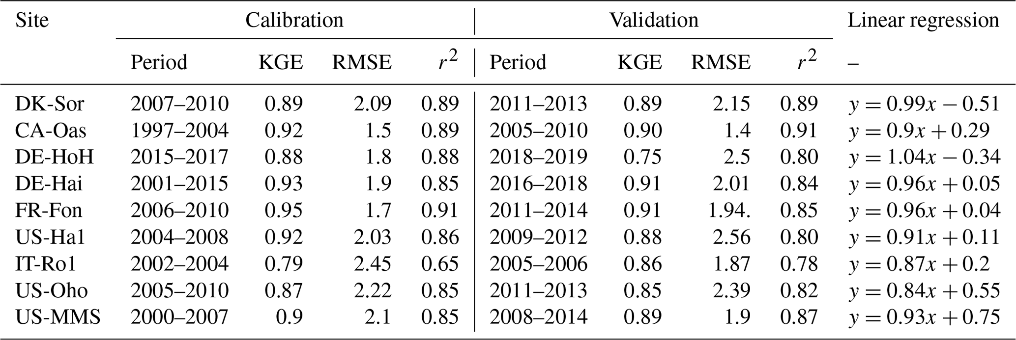
We conduct site-specific parameter estimation for all available eddy covariance (EC) flux tower study sites (Fig. 5). For this, only the most sensitive parameters (depending on the sensitivity analysis result at each site, the number of the most sensitive parameters varied between 8 and 14 parameters) identified in the sensitivity analysis are calibrated, and the others are fixed (Table 3). For model parameter calibrations, we used the first half of the available time series and the remaining years for validation (Table 1). Calibration and validation of the model are only performed for the GPP flux, because direct LAI measurements are not available at all of the flux sites. Figure 5 shows the seven-day mean of simulated GPP for a set of ensemble members for each study site during both the calibration and validation periods. Since the different sites were operational at different times and since some sites (e.g., DE-Hai) cover a relatively long time period, we show only 5 years of simulation at each site: the last 3 years of calibration and the first 2 years of validation (Fig. 5). A complete simulation for each site during the entire available times series is provided in Fig. S4 in the Supplement. In addition, Table 4 summarizes the model performance in simulating GPP during the calibration and validation periods at different sites. In general, the model achieved KGE values of above 0.65, RMSE of less than 2.5 , and r2 values of above 0.65 over all study sites. We compare the performance of our model to other modeling studies whenever there is either an identical site or a similar biome type (i.e., DBF) to our study presented. To this end, our results are similar to Yue and Unger (2015), who found a high correlation of more than 0.8 and RMSE lower than 3 for the GPP simulations at DBF forest sites in a global setting using the Yale Interactive terrestrial Biosphere model. Another study conducted by Asaadi et al. (2018) showed a quite good model performance using the CLASS-CTEM land surface model (Melton and Arora, 2014) applied at US-Ha1 (1998–2013) and US-MMs (1999–2006) flux tower sites, with an r2 value of 0.99 accompanying RMSE of 0.62 and an r2 value of 0.98 accompanying RMSE of 1.07 at US-Ha1 and US-MMs, respectively. In a recent study, Holtmann et al. (2021) assessed the daily carbon fluxes over the DE-HoH forest during 2015–2017 using the FORMIND model (Fischer et al., 2016). They showed that the simulated and measured GPP correlates with an r2 of 0.82 and RMSE of 9 equivalent to 2.46 using the FORMIND model.
Table 4Summary statistics for the comparison between model-estimated GPP and tower-estimated GPP at different sites. Statistics include KGE, root-mean-square error (RMSE), and r2. GPP units are []. The statistics refer to ensemble medians of model-estimated GPP. The linear regression is over both the calibration and validation periods.
Taken together, our model exhibits a reasonable performance and performs equally well in estimating the temporal dynamics of GPP (Table 4) compared to other, more complex land surface and biogeochemical models. The PCM shows skill in capturing GPP at most of the investigated sites, although it overestimates GPP at the IT-Ro1 during summer. IT-Ro1 is located in a Mediterranean climate exposed to dry summers (Vicca et al., 2016). The forest ecosystems in Mediterranean-type climates are affected by water limitations that can affect the GPP flux significantly (Cueva et al., 2021). The lack of soil moisture data probably contributed to the misrepresentation of GPP at this site. This is in agreement with previous studies that found similarly poor modeling performance across sites located in the Mediterranean climate in central Italy in dry summer periods when simulating GPP (Maselli et al., 2012; Chiesi et al., 2011; Fibbi et al., 2019). Vargas et al. (2013) also discussed the interannual dynamics of the effect of soil moisture on GPP flux in Mediterranean ecosystems using five process-oriented ecosystem models, including water balance. They observed a systematic underestimation of GPP in the models that were accounting for soil water balance. Those underestimations may have been related to the complex nature of Mediterranean ecosystems, e.g., due to deep roots and the important role of the lower canopy. In contrast, here we overestimate the GPP and believe that this is due to lack of local information on soil moisture stress. More information regarding soil moisture stress is therefore expected to improve the model. Overall, they emphasize the importance of drought conditions and the complex nature of Mediterranean ecosystems in representing forest dynamics, including GPP flux. In addition, the impact of water limitation on GPP could be related to the irregular occurrence of extreme events (e.g., the European-wide drought in 2018). Such conditions were observed at DE-HoH and DE-Hai sites, where the model overestimated GPP during the late summer of 2018, which coincided with the Europe-wide drought of 2018 (Buras et al., 2020). In the next step, we also examined the model's overall performance in reproducing GPP in terms of the multi-year average of GPP at each site. Figure 6 shows that the model can generally explain the spatial variation of GPP with an r2 as high as 0.90.
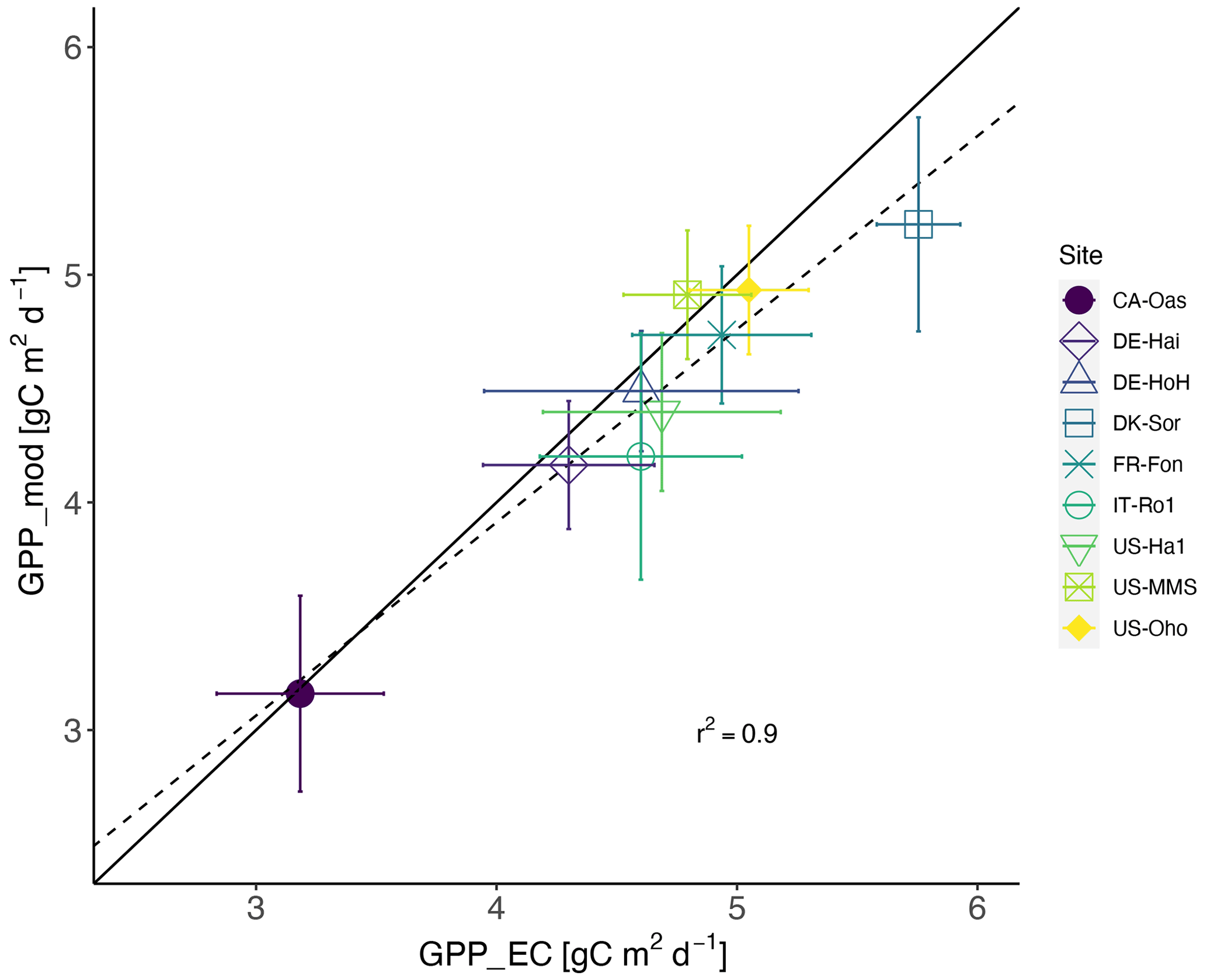
Figure 6Estimated GPP based on flux tower measurements vs. modeled GPP ± 1 standard deviation (error bars) across the 9 studied sites. The solid line indicates the 1:1 line, and the dashed line indicates the regression line. Each dot represents one of the sites and refers to site-averaged GPP over the entire available time series.
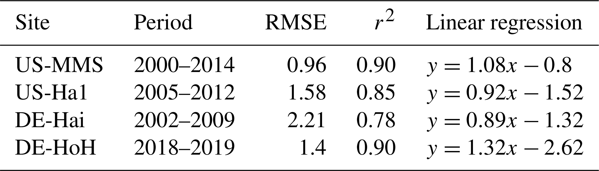
As an independent validation step, we evaluate the PCM simulations of LAI against field-measurement data from some study sites where observational data were made available via personal contacts with site investigators. Figure 7 compares the simulated values of LAI with their field measurements at four sites (US-MMS, US-Ha1, DE-Hai, and DE-HoH). In general, a good spatial and temporal consistency between the simulated LAI and the field-measurement LAI can be seen from the plots (Fig. 7). The r2 corresponding to the US-MMS, US-Ha1, DE-Hai, and DE-HoH sites are 0.90, 0.85, 0.78, and 0.90, respectively. Furthermore, the comparisons yield RMSE of 0.96, 1.58, 2.21, 1.4 m2 m−2 to the US-MMS, US-Ha1, DE-Hai, and DE-HoH sites, respectively. Table 5 summarizes the model performance in simulating LAI during a common period of observed and modeled data.
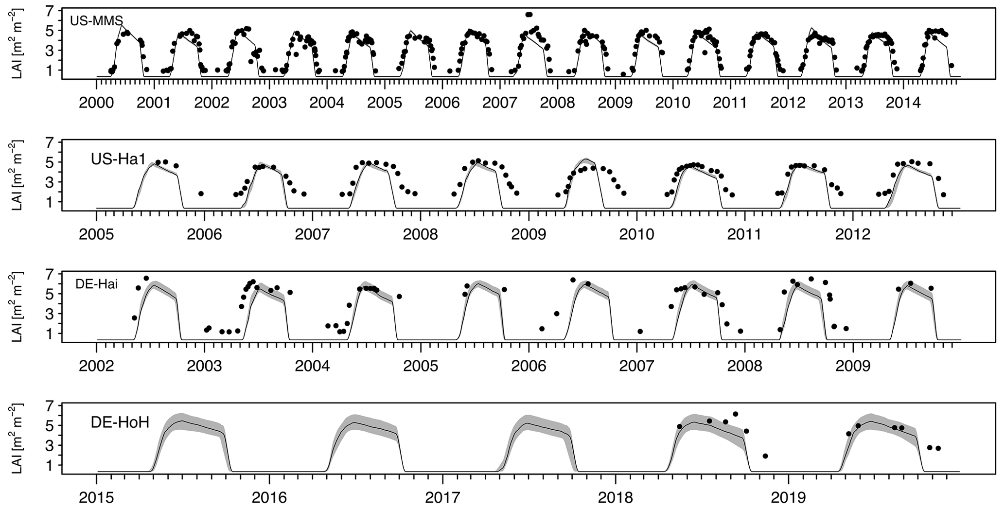
Figure 7Time series of observed and simulated LAI at study flux tower sites during the common years of field measurements and simulations. The black dots indicate the field measurement LAI. The light gray, shaded area corresponds to ensemble members of the LAI output at each time step. The dark gray line refers to the median of ensemble members.
Table 5Summary statistics for the comparison between model-estimated LAI and field measurement LAI at different sites. Statistics include r2 and RMSE. LAI units are []. The statistics refer to ensemble medians of model-estimated LAI.
The simulated LAI captures the observed LAI seasonality at almost all the sites reasonably well. It demonstrates the capability of the model in capturing the canopy status at different phenophases. However, there are some pronounced deviations between modeled and observed LAI at some sites (US-Ha1, DE-HoH) during the dormancy phase and autumn leaf decline period. Given the deciduous nature of those ecosystems, it is likely that the higher winter values of the field measurements compared to the simulated LAI reflects the presence of understory vegetation (Asaadi et al., 2018) or the instrument's reading of present stand and/or dead leaves on trees after the onset of leaf shedding. We also notice a slight phase of lag in the simulated LAI during the spring as compared to the field measurements data (e.g., at the DE-Hai site). Such discrepancy may be due to the lack of accounting for the dependence of the green-up rate on non-structural carbohydrates from previous years as a buffer to initiate leaf onset (Asaadi et al., 2018), which is currently not represented in the PCM.
3.3 Spatial model validation and model generalization
We conduct a cross-validation of the parameter transferability for all sites against tower-derived GPP data (Sect. 2.2.5). Figure 8 summarizes the results of this analysis, providing a comparison between the range of obtained Kling–Gupta efficiency performance metrics (KGE) from on-site calibrations and KGE obtained from a compromised solution. It can be seen that the model with a compromise parameter set still shows a reasonable predictive skill (KGE>0.5) while leaving space for skill improvement with a site-specific parameter (ΔKGE≈0.10). The poorest performances are associated with the northernmost site, DK-Sor, and the Mediterranean IT-Ro1 site. The associated bias in those sites is likely related to GPP response to the maximum LUE parameter obtained from the compromise solution applied over all the sites. As was shown in the sensitivity analysis (see Sect. 3.1.1), the variation of GPP is predominantly driven by the LUE variation; thus, a constant, fixed maximum LUE across all sites might be a reason for the limited performance at the sites located in maximum latitude and water-limited regions. It has been shown that maximum LUE varies in different geographical locations (Jung et al., 2007), and this is in line with our on-site calibration result indicating largest maximum LUE at the DK-Sor (northernmost site with a cold and moist climate) and lowest at the IT-Ro1 (a relatively drier, Mediterranean site) sites. Thus, applying a compromise value for LUE at these two sites would result in a bias in GPP estimation. Previous studies (Wang et al., 2010; Madani et al., 2014) showed a large variation in maximum LUE not only between different biomes but also within an individual biome and plant functional type. Concerning the large spatial variability of maximum LUE, several factors – such as the spatial heterogeneity of vegetation, canopy densities, ages, soil nutrition, and leaf nutrient content – have been mentioned in previous studies (Wang et al., 2010; Madani et al., 2014). Some methods, such as spatially explicit estimation of optimum LUE (Madani et al., 2014) or the introduction of pixel-level maximum LUE (Wang et al., 2010), have been employed in satellite-based LUE models to overcome this shortcoming. It is argued that the assumption of a constant maximum LUE (i.e., based on a standard MODIS-based GPP algorithm and a biome property look-up table; Heinsch et al., 2003) needs to be re-examined so that spatial heterogeneity between individual plant functional types is represented. Therefore, the uncertainty introduced by the fixed maximum LUE may be reduced and ecosystem productivity modeling would be improved.
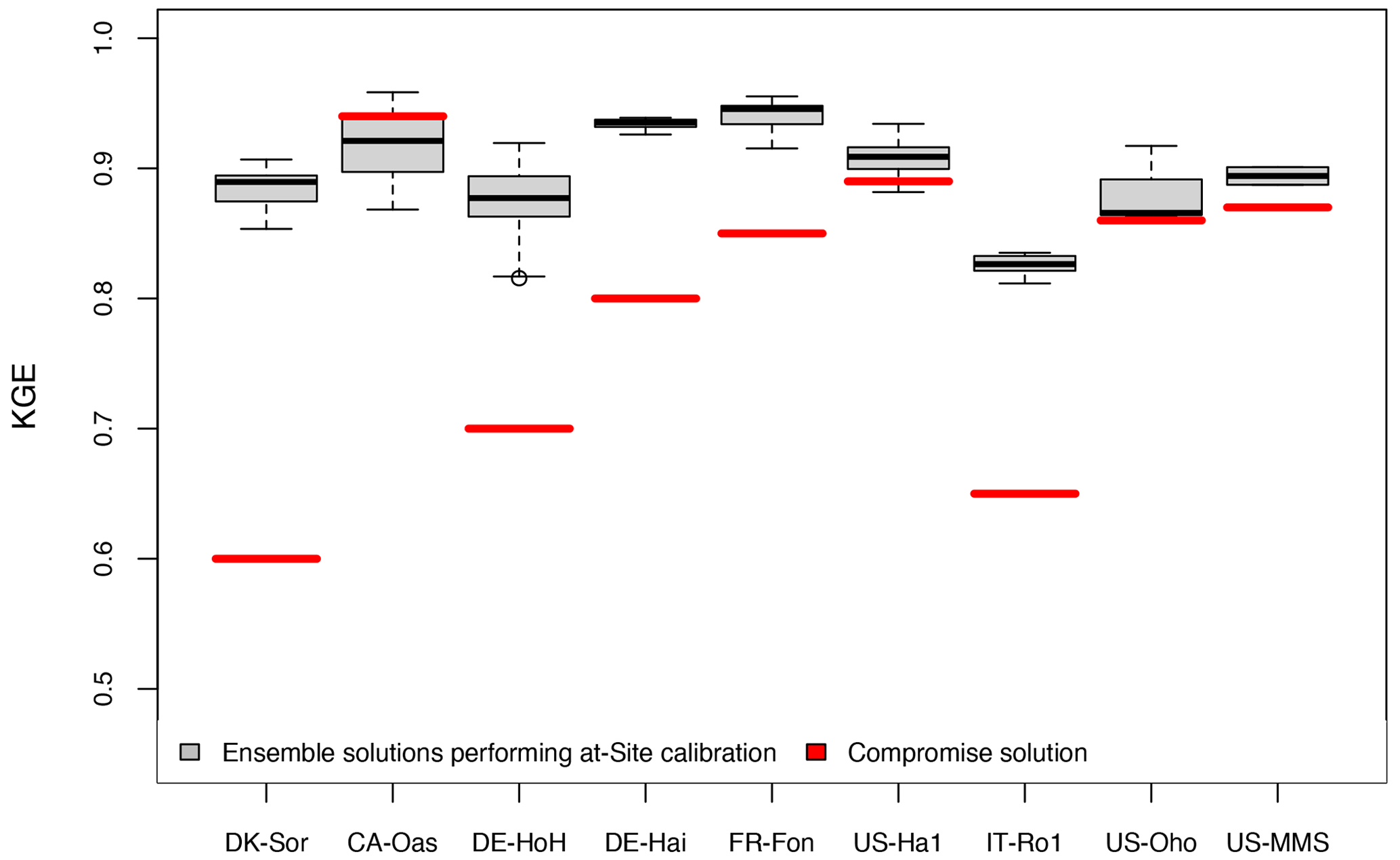
Figure 8Comparison between KGE obtained from ensemble-simulated GPP performing at-site calibration, and the KGE obtained from compromised solution.
3.4 Limitations and opportunities
While the model performs well, in general, in simulating the GPP, some inconsistencies in the observed and modeled GPP across sites help to identify the model's limitations and introduce future opportunities to improve the model's performance. One of the limitations is that the model was unable to adequately capture the observed decline in GPP in 2019 (Fig. 5) at the DE-HoH. This may be related to a possible legacy impact of the drought year 2018 on the successive year 2019 (Buras et al., 2020; Schuldt et al., 2020; Schnabel et al., 2021; Reichstein et al., 2013). Here, we infer that the reduction in the tower GPP in 2019 might be due to a change in the LUE parameter. Based on calibration from previous non-drought years, the obtained LUE value might lead the model to overestimate GPP in early 2019. Indeed, calibrating the model to the drought years of 2018 and 2019 yielded a lower LUE parameter (reduction of LUE value by 12 %), which might support the possible legacy impact of last year's drought on the LUE parameter. Another possible explanation, alternatively to or collectively with the plant legacy effect, would be the variation in or depletion of deep soil moisture storage (Jung et al., 2009). Since the model does not represent established internal feedback for carry-over effects after extreme events (Reichstein et al., 2013) and only considers the soil moisture up to 80 cm depth, the current model version would not reflect on such a process, and GPP is likely to be overestimated.
Another limitation in our simulation is that the possible effect of diffuse light on GPP response is not accounted for in the current model structure. We observed the potential role of diffuse light on GPP during some mismatch periods between eddy flux tower and modeled GPP across some of the sites (e.g., DE-HoH year 2017, FR-Fon year 2012, and US-Ha1 year 2010) (see Fig. S1). The model underestimates GPP during these periods based on a lower PAR input; however, the observations show greater GPP despite lower input PAR. This is in line with the findings of Knohl and Baldocchi (2008), who investigated the effect of diffuse light on the forest ecosystem and discussed how diffuse radiation can lead to an increase in carbon uptake. The enhancement of GPP due to diffuse light is related to a more even distribution and more efficient light penetration within the canopy (Yuan et al., 2014). Integration of such effects in the current model by means of introducing a time-varying LUE (condition-varying) (Wei et al., 2017) instead of the fixed LUE would improve the simulation result. In particular, under unprecedented global warming and climate change, future changes in cloud cover and aerosol concentrations are expected to modify the solar radiation and the subsequent ecosystem productivity (Durand et al., 2021; Meyer et al., 2014). Regarding LAI simulation, one limitation is that, at some points, the model cannot increase LAI in the initial onset of LAI as fast as that which is observed in the early growing period. In previous studies, it has been shown that the inclusion of non-structural carbon storage at the beginning of green-up might help to overcome this issue (Asaadi et al., 2018) and refine the model simulation results further. Aside from the current model limitations to be subjected to further improvement, the model exhibits a reasonable validity and performs equally well in estimating the temporal dynamics of GPP and LAI development compared to more complex land surface and biogeochemical models. The PCM being parsimonious makes it suitable for more far-reaching applications in coupled models. Dynamic development of LAI is relevant to GPP estimation and is beneficial for hydrologic models, providing them with prognostically driven LAI time series based on vegetation responses to temperature, particularly in the context of water budget responses to climate variability.
We aim, as a next step, to implement the presented model into the existing open-source mesoscale Hydrologic Model (mHM; Samaniego et al., 2010; Kumar et al., 2013, available at https://www.ufz.de/mhm, last access: 20 March 2022), with a proven predictive power in simulating root-zone soil moisture dynamics (Boeing et al., 2021). The spatially simulated soil moisture derived from mHM would provide an alternative to the (limited) soil moisture observations required for GPP simulation. In particular, in the face of ongoing and future climate changes and the increasing occurrence of droughts (Harper et al., 2021), reliable simulations of soil moisture are invaluable information for capturing plant drought responses for the carbon cycle and climate feedbacks (Harper et al., 2021). Finally, in doing so, we expect the improved capability of the hydrological model to represent the coupled water and carbon (i.e., GPP/LAI in this study) components.
In view of ongoing natural and anthropogenic changes, assessing the extent to which terrestrial plants can sequester atmospheric carbon and affect the water balance through LAI is essential for effective climate-adaptation and resilience plans. Here, we present a parsimonious canopy model (PCM) with a medium level of complexity to simulate canopy GPP and LAI. In the PCM model, the carbon uptake drives leaf biomass accumulation based on a mass balance approach. The model employs the light use efficiency principle, in which the core concept is the conversion of absorbed photosynthetically active radiation (PAR) into biomass. An integrated phenology submodel, from which the allocation of carbon to and decay from the leaf pool is guided, is incorporated to predict the timing of leaf development and to characterize different phenological stages. The PCM model performed reasonably well in reproducing the daily development of GPP and LAI in deciduous broad-leaved forest biomes across Europe and North America. The model runs with a few required inputs: air temperature, vapor pressure deficit, PAR, and soil moisture (optional, though recommended in dry regions and drought events). Although the proposed model runs with a number of parameters for representing the relevant processes (29 parameters without the soil moisture-related parameters), a global sensitivity analysis showed that only 10 parameters (on average across sites) were sensitive and had to be inferred via calibration. The result reaffirms that light use efficiency and specific leaf area index parameters are by far the most informative parameters in GPP and LAI simulations, respectively. The on-site calibrated maximum LUE parameter showed relatively large variation within the sites, with greater maximum LUE in Denmark (Dk-Sor site) and lower values in Italy (IT-Ro1 site). It implies that applying a fixed, biome-specific, maximum LUE would not be applicable over different locations. Moreover, modeled GPP during the growing season was shown to be almost insensitive to LAI changes. This indicates that GPP is saturated at a particular value of LAI, and any further increase in LAI does not necessarily increase the resultant GPP. We also tested the robustness and generality of the underlying model structure, identifying a compromise set of model parameters applicable to all sites (region-wide). The results show that the model application is possible without site-specific calibration while still yielding reasonable model quality. The model's skill in capturing the LAI dynamics – which were not used in the parameter inference process – further confirms the robustness of the presented model structure. Given the scarce soil moisture information, we expect that simulated soil moisture derived from a hydrological model would improve the representation of GPP simulations, particularly at semiarid regions or during drought events. We envision that the medium complexity of the presented model will allow for a seamless integration into large-scale hydrological models to better represent the ecohydrological aspects of ecosystems. We plan to implement the PCM model into the existing hydrologic models (e.g., open-source mesoscale Hydrologic Model; mHM), thereby enabling an improved representation of coupled water and carbon fluxes in the face of a changing environment. To allow for a seamless estimation of carbon and water fluxes, we plan to include the implementation of a robust, regional parameter inference approach (e.g., establishing regionalized LUE parameters through a multiscale parameterization approach; Samaniego et al., 2010) and performing extensive cross-validation experiments to ensure credible model simulations across a wide range of spatial domains.
The PCM is archived at https://doi.org/10.5281/zenodo.6373776 (Bahrami et al., 2022) (last access: 21 March 2022). It is also publicly available at https://git.ufz.de/bahrami/pcm (last access: 21 March 2022).
The flux tower datasets for DK-Sor, CA-Oas, DE-Hai, FR-Fon, IT-Ro1, US-Ha1, US-Oho, and US-MMS can be can be accessed from the FLUXNET 2015 Tier 1 at https://fluxnet.org/data/fluxnet2015-dataset/ (last access: 20 July 2021). Data from DE-HoH are available from corinna.bebmann@ufz.de and felix.pohl@ufz.de. LAI field measurements for US-Ha1 can be downloaded from https://harvardforest1.fas.harvard.edu/exist/apps/datasets/showData.html?id=hf069 (last access: 20 January 2022)
The supplement related to this article is available online at: https://doi.org/10.5194/gmd-15-6957-2022-supplement.
BB coded and scripted the model. BB performed the sensitivity analysis. BB also prepared the manuscript. RK, AH, and ST were involved in the interpretation of the results and discussions. All authors contributed to the results, discussion, review, and editing of the manuscript.
The contact author has declared that none of the authors has any competing interests.
Publisher's note: Copernicus Publications remains neutral with regard to jurisdictional claims in published maps and institutional affiliations.
We acknowledge the FLUXNET data network for providing the data at participant flux sites – DK-Sor, CA-Oas, DE-Hai, FR-Fon, US-Ha1, US-Oho, US-MMS, IT-Ro1 – used in our study. We would like to thank Felix Pohl for providing data from the DE-HoH flux site. We thank Anne Klosterhalfen for the helpful information regarding the data for DE-Hai. We would also like to thank Corinna Rebmann (DE-HoH), Martina Mund (DE-Hai), Timothy Whitby (US-Ha1), and Michael Phillip Voyles (US-MMS) for sharing the LAI data in this study.
The article processing charges for this open-access publication were covered by the Helmholtz Centre for Environmental Research – UFZ.
This paper was edited by David Lawrence and reviewed by two anonymous referees.
Ariza-Carricondo, C., Mauro, F., Op de Beeck, M., Roland, M., Gielen, B., Vitale, D., Ceulemans, R., and Papale, D.: A comparison of different methods for assessing leaf area index in four canopy types, Central European Forestry Journal, 65, 67–80, https://doi.org/10.2478/forj-2019-0011, 2019. a, b, c
Arora, V.: Modeling vegetation as dynamic component in soil-vegetation-atmosphere transfer schemes and hydrological models, Rev. Geophys., 40, 1–26, https://doi.org/10.1029/2001RG000103, 2002. a, b, c
Arsenault, K., Nearing, G., Wang, S., Yatheendradas, S., and Peters-Lidard, C.: Parameter Sensitivity of the Noah-MP Land Surface Model with Dynamic Vegetation, J. Hydrometeorol., 19, 815–830, https://doi.org/10.1175/JHM-D-17-0205.1, 2018. a, b
Asaadi, A., Arora, V. K., Melton, J. R., and Bartlett, P.: An improved parameterization of leaf area index (LAI) seasonality in the Canadian Land Surface Scheme (CLASS) and Canadian Terrestrial Ecosystem Model (CTEM) modelling framework, Biogeosciences, 15, 6885–6907, https://doi.org/10.5194/bg-15-6885-2018, 2018. a, b, c, d, e
Balzarolo, M., Valdameri, N., Fu, Y. H., Schepers, L., Janssens, I. A., and Campioli, M.: Different determinants of radiation use efficiency in cold and temperate forests, Global Ecol. Biogeogr., 28, 1649–1667, https://doi.org/10.1111/geb.12985, 2019. a
Beer, C., Reichstein, M., Tomelleri, E., Ciais, P., Jung, M., Carvalhais, N., Rodenbeck, C., Arain, M., Baldocchi, D., Bonan, G., Bondeau, A., Cescatti, A., Lasslop, G., Lindroth, A., Lomas, M., Luyssaert, S., Margolis, H., Oleson, K., Roupsard, O., and Papale, D.: Terrestrial Gross Carbon Dioxide Uptake: Global Distribution and Covariation with Climate, Science, 329, 834–838, https://doi.org/10.1126/science.1184984, 2010. a, b
Boeing, F., Rakovech, O., Kumar, R., Samaniego, L., Schrön, M., Hildebrandt, A., Rebmann, C., Thober, S., Müller, S., Zacharias, S., Bogena, H., Schneider, K., Kiese, R., and Marx, A.: High-resolution drought simulations and comparison to soil moisture observations in Germany, Hydrol. Earth Syst. Sci. Discuss. [preprint], https://doi.org/10.5194/hess-2021-402, in review, 2021. a
Bohn, F. J., Frank, K., and Huth, A.: Of climate and its resulting tree growth: Simulating the productivity of temperate forests, Ecol. Model., 278, 9–17, https://doi.org/10.1016/j.ecolmodel.2014.01.021, 2014. a
Bonhomme, R. and Chartier, P.: The interpretation and automatic measurement of hemispherical photographs to obtain sunlit foliage area and gap frequency, Israel J. Agr. Res., 22, 53–61, 1972. a
Boons-Prins, E.: Grassland simulation with the LPJmL model: version 3.4.018, no. 172 in WOt-werkdocument, Wettelijke Onderzoekstaken Natuur and Milieu, 2010. a
Buras, A., Rammig, A., and Zang, C. S.: Quantifying impacts of the 2018 drought on European ecosystems in comparison to 2003, Biogeosciences, 17, 1655–1672, https://doi.org/10.5194/bg-17-1655-2020, 2020. a, b
Che, M.-L., Chen, B.-Z., Wang, Y., and Guo, X.-Y.: Review of dynamic global vegetation models (DGVMs), J. Appl. Ecol., 25, 263–271, 2014. a
Cheng, Y.-B., Zhang, Q., Lyapustin, A., Wang, Y., and Middleton, E.: Impacts of light use efficiency and fPAR parameterization on gross primary production modeling, Agr. Forest Meteorol., 189–190, 187–197, https://doi.org/10.1016/j.agrformet.2014.01.006, 2014. a, b, c
Chiesi, M., Fibbi, L., Genesio, L., Gioli, B., Magno, R., Maselli, F., Moriondo, M., and Vaccari, F.: Integration of ground and satellite data to model Mediterranean forest processes, Int. J. Appl. Earth Obs., 13, 504–515, https://doi.org/10.1016/j.jag.2010.10.006, 2011. a
Cholet, C., Houle, D., Sylvain, J.-D., Doyon, F., and Maheu, A.: Climate Change Increases the Severity and Duration of Soil Water Stress in the Temperate Forest of Eastern North America, Frontiers in Forests and Global Change, 5, 879382, https://doi.org/10.3389/ffgc.2022.879382, 2022. a
Collatz, G., Ribas-Carbo, M., and Berry, J.: Coupled Photosynthesis-Stomatal Conductance Model for Leaves of C4 Plants, Funct. Plant Biol., 19, 519–538, https://doi.org/10.1071/PP9920519, 1992. a
Coops, N. C., Waring, R. H., and Law, B. E.: Assessing the past and future distribution and productivity of ponderosa pine in the Pacific Northwest using a process model, 3-PG, Ecol. Model., 183, 107–124, https://doi.org/10.1016/j.ecolmodel.2004.08.002, 2005. a
Cox, P., Betts, R., Bunton, C., Essery, R., Rowntree, P., and Smith, J.: The impact of new land surface physics on the GCM simulation of climate and climate sensitivity, Clim. Dynam., 15, 183–203, https://doi.org/10.1007/s003820050276, 1999. a
Cueva, A., Bullock, S. H., Méndez-Alonzo, R., López-Reyes, E., and Vargas, R.: Foliage Senescence as a Key Parameter for Modeling Gross Primary Productivity in a Mediterranean Shrubland, J. Geophys. Res.-Biogeo., 126, e2020JG005839, https://doi.org/10.1029/2020JG005839, 2021. a
Cuntz, M., Mai, J., Samaniego, L., Clark, M., Wulfmeyer, V., Branch, O., Attinger, S., and Thober, S.: The impact of standard and hard-coded parameters on the hydrologic fluxes in the Noah-MP land surface model, J. Geophys. Res.-Atmos., 121, 10676–10700, https://doi.org/10.1002/2016JD025097, 2016. a, b
Durand, M., Murchie, E. H., Lindfors, A. V., Urban, O., Aphalo, P. J., and Robson, T. M.: Diffuse solar radiation and canopy photosynthesis in a changing environment, Agr. Forest Meteorol., 311, 108684, https://doi.org/10.1016/j.agrformet.2021.108684, 2021. a
Dyderski, M. K., Chmura, D., Dylewski, Ł., Horodecki, P., Jagodziński, A. M., Pietras, M., Robakowski, P., and Woziwoda, B.: Biological Flora of the British Isles: Quercus rubra, J. Ecol., 108, 1199–1225, https://doi.org/10.1111/1365-2745.13375, 2020. a
Estoque, R., Dasgupta, R., Winkler, K., Avitabile, V., Johnson, B., Myint, S., Gao, Y., Ooba, M., Murayama, Y., and Lasco, R.: Spatiotemporal pattern of global forest change over the past 60 years and the forest transition theory, Environ. Res. Lett., 17, 084022, https://doi.org/10.1088/1748-9326/ac7df5, 2022. a
Fang, H., Baret, F., Plummer, S., and Schaepman-Strub, G.: An Overview of Global Leaf Area Index (LAI): Methods, Products, Validation, and Applications, Rev. Geophys., 57, 739–799, https://doi.org/10.1029/2018RG000608, 2019. a, b, c
Farquhar, G. D., von Caemmerer, S., and Berry, J. A.: A biochemical model of photosynthetic CO2 assimilation in leaves of C3 species, Planta, 149, 78–90, https://doi.org/10.1007/BF00386231, 1980. a, b
Fibbi, L., Moriondo, M., Chiesi, M., Bindi, M., and Maselli, F.: Impacts of climate change on the gross primary production of Italian forests, Ann. For. Sci., 76, 59, https://doi.org/10.1007/s13595-019-0843-x, 2019. a
Fischer, R., Armstrong, A., Shugart, H. H., and Huth, A.: Simulating the impacts of reduced rainfall on carbon stocks and net ecosystem exchange in a tropical forest, Environ. Modell. Softw., 52, 200–206, https://doi.org/10.1016/j.envsoft.2013.10.026, 2014. a
Fischer, R., Bohn, F., Dantas de Paula, M., Dislich, C., Groeneveld, J., Gutiérrez, A. G., Kazmierczak, M., Knapp, N., Lehmann, S., Paulick, S., Pütz, S., Rödig, E., Taubert, F., Köhler, P., and Huth, A.: Lessons learned from applying a forest gap model to understand ecosystem and carbon dynamics of complex tropical forests, Ecol. Model., 326, 124–133, https://doi.org/10.1016/j.ecolmodel.2015.11.018, 2016. a, b, c, d, e, f
Fleischer, K., Rebel, K. T., van der Molen, M. K., Erisman, J. W., Wassen, M. J., van Loon, E. E., Montagnani, L., Gough, C. M., Herbst, M., Janssens, I. A., Gianelle, D., and Dolman, A. J.: The contribution of nitrogen deposition to the photosynthetic capacity of forests, Global Biogeochem. Cy., 27, 187–199, https://doi.org/10.1002/gbc.20026, 2013. a, b, c, d
Foley, J. and Ramankutty, N.: A primer on the terrestrial carbon cycle: What we don't know but should, in: The global carbon cycle: integrating humans, climate, and the natural world, edited by: Field, C. B. and Raupach, M. R., Island Press, Washington, D.C., 279–294, 2003. a
Forzieri, G., Girardello, M., Ceccherini, G., Spinoni, J., Feyen, L., Hartmann, H., Beck, P. S. A., Camps-Valls, G., Chirici, G., Mauri, A., and Cescatti, A.: Emergent vulnerability to climate-driven disturbances in European forests, Nat. Commun., 12, 1081, https://doi.org/10.1038/s41467-021-21399-7, 2021. a
Francés, F., Velez, J., and Velez, J.: Split-parameter structure for the automatic calibration of distributed hydrological models, J. Hydrol., 332, 226–240, https://doi.org/10.1016/j.jhydrol.2006.06.032, 2007. a, b
Friedlingstein, P., Joel, G., Field, C. B., and Fung, I. Y.: Toward an allocation scheme for global terrestrial carbon models, Glob. Change Biol., 5, 755–770, https://doi.org/10.1046/j.1365-2486.1999.00269.x, 1999. a
Frost-Christensen, H. and Sand-Jensen, K.: The quantum efficiency of photosynthesis in macroalgae and submerged angiosperms, Oecologia, 91, 377–384, https://doi.org/10.1007/BF00317627, 1992. a
Gamon, J. A.: Reviews and Syntheses: optical sampling of the flux tower footprint, Biogeosciences, 12, 4509–4523, https://doi.org/10.5194/bg-12-4509-2015, 2015. a
Gim, H.-J., Park, S. K., Kang, M., Thakuri, B. M., Kim, J., and Ho, C.-H.: An improved parameterization of the allocation of assimilated carbon to plant parts in vegetation dynamics for Noah-MP, J. Adv. Model. Earth Sy., 9, 1776–1794, https://doi.org/10.1002/2016MS000890, 2017. a, b, c, d
Göhler, M., Mai, J., and Cuntz, M.: Use of eigendecomposition in a parameter sensitivity analysis of the Community Land Model, J. Geophys. Res.-Biogeo., 118, 904–921, https://doi.org/10.1002/jgrg.20072, 2013. a
Gower, S. and Norman, J.: Rapid Estimation of Leaf Area Index in Conifer and Broad-Leaf Plantations, Ecology, 72, 1896–1900, https://doi.org/10.2307/1940988, 1991. a
Granier, A., Bréda, N., Biron, P., and Villette, S.: A lumped water balance model to evaluate duration and intensity of drought constraints in forest stands, Ecol. Model., 116, 269–283, https://doi.org/10.1016/S0304-3800(98)00205-1, 1999. a, b, c, d
Granier, A., Ceschia, E., Damesin, C., Dufrêne, E., Epron, D., Gross, P., Lebaube, S., Le Dantec, V., Le Goff, N., Lemoine, D., Lucot, E., Ottorini, J. M., Pontailler, J. Y., and Saugier, B.: The carbon balance of a young Beech forest, Funct. Ecol., 14, 312–325, https://doi.org/10.1046/j.1365-2435.2000.00434.x, 2000. a
Guan, X., Chen, J., Shen, H., and Xie, X.: A modified two-leaf light use efficiency model for improving the simulation of GPP using a radiation scalar, Agric. Forest Meteorol., 307, 108546, https://doi.org/10.1016/j.agrformet.2021.108546, 2021. a
Gupta, H., Kling, H., Yilmaz, K., and Martinez, G.: Decomposition of the Mean Squared Error and NSE Performance Criteria: Implications for Improving Hydrological Modelling, J. Hydrol., 377, 80–91, https://doi.org/10.1016/j.jhydrol.2009.08.003, 2009. a
Harper, A. B., Williams, K. E., McGuire, P. C., Duran Rojas, M. C., Hemming, D., Verhoef, A., Huntingford, C., Rowland, L., Marthews, T., Breder Eller, C., Mathison, C., Nobrega, R. L. B., Gedney, N., Vidale, P. L., Otu-Larbi, F., Pandey, D., Garrigues, S., Wright, A., Slevin, D., De Kauwe, M. G., Blyth, E., Ardö, J., Black, A., Bonal, D., Buchmann, N., Burban, B., Fuchs, K., de Grandcourt, A., Mammarella, I., Merbold, L., Montagnani, L., Nouvellon, Y., Restrepo-Coupe, N., and Wohlfahrt, G.: Improvement of modeling plant responses to low soil moisture in JULESvn4.9 and evaluation against flux tower measurements, Geosci. Model Dev., 14, 3269–3294, https://doi.org/10.5194/gmd-14-3269-2021, 2021. a, b, c
Hartge, K. H.: Feddes, R. A., Kowalik, P. I. und Zaradny, H.: simulation of field water use and crop yield. Pudoc (Centre for agricultural publishing and documentation) Wageningen, Niederlande, 195 Seiten, 13 Abbildungen, Paperback. Preis: hfl 30,–, Z. Pflanz. Bodenkunde, 143, 254–255, https://doi.org/10.1002/jpln.19801430219, 1980. a
Haverd, V., Smith, B., Raupach, M., Briggs, P., Nieradzik, L., Beringer, J., Hutley, L., Trudinger, C. M., and Cleverly, J.: Coupling carbon allocation with leaf and root phenology predicts tree–grass partitioning along a savanna rainfall gradient, Biogeosciences, 13, 761–779, https://doi.org/10.5194/bg-13-761-2016, 2016. a
Heinsch, F., Reeves, M., Votava, P., Kang, S., Cristina, M., Zhao, M., Glassy, J., Jolly, W., Loehman, R., Bowker, C., Kimball, J., and Nemani, R.: User's guide GPP and NPP (MOD17A2/A3) products NASA MODIS land algorithm, Version 2.0, 2003. a, b, c
Hidy, D., Barcza, Z., Hollós, R., Dobor, L., Ács, T., Zacháry, D., Filep, T., Pásztor, L., Incze, D., Dencső, M., Tóth, E., Merganičová, K., Thornton, P., Running, S., and Fodor, N.: Soil-related developments of the Biome-BGCMuSo v6.2 terrestrial ecosystem model, Geosci. Model Dev., 15, 2157–2181, https://doi.org/10.5194/gmd-15-2157-2022, 2022. a, b
Hirmas, D., Giménez, D., Nemes, A., Kerry, R., Brunsell, N., and Wilson, C.: Climate-induced changes in continental-scale soil macroporosity may intensify water cycle, Nature, 561, 100–103, https://doi.org/10.1038/s41586-018-0463-x, 2018. a
Holtmann, A., Huth, A., Pohl, F., Rebmann, C., and Fischer, R.: Carbon Sequestration in Mixed Deciduous Forests: The Influence of Tree Size and Species Composition Derived from Model Experiments, Forests, 12, 726, https://doi.org/10.3390/f12060726, 2021. a
Hou, Z., Huang, M., Leung, L. R., Lin, G., and Ricciuto, D. M.: Sensitivity of surface flux simulations to hydrologic parameters based on an uncertainty quantification framework applied to the Community Land Model, J. Geophys. Res.-Atmos., 117, D15108, https://doi.org/10.1029/2012JD017521, 2012. a
Huang, X., Zheng, Y., Zhang, H., Lin, S., Liang, S., Li, X., Ma, M., and Yuan, W.: High spatial resolution vegetation gross primary production product: Algorithm and validation, Science of Remote Sensing, 5, 100049, https://doi.org/10.1016/j.srs.2022.100049, 2022. a
Imadi, S., Gul, A., Dikilitas, M., Karakas, S., Sharma, I., and Ahmad, P.: Water stress: Types, causes, and impact on plant growth and development, John Wiley & Sons, 343–355, https://doi.org/10.1002/9781119054450.ch21, 2016. a
Iooss, B. and Lemaître, P.: A Review on Global Sensitivity Analysis Methods, Operations Research/Computer Science Interfaces Series, vol. 59, Springer, https://doi.org/10.1007/978-1-4899-7547-8_5, 2014. a
IPCC: Climate Change 2021: The Physical Science Basis. Contribution of Working Group I to the Sixth Assessment Report of the Intergovernmental Panel on Climate Change, edited by: Masson-Delmotte, V., Zhai, P., Pirani, A., Connors, S. L., Péan, C., Berger, S., Caud, N., Chen, Y., Goldfarb, L., Gomis, M. I., Huang, M., Leitzell, K., Lonnoy, E., Matthews, J. B. R., Maycock, T. K., Waterfield, T., Yelekçi, O., Yu, R., and Zhou, B., Cambridge University Press, in press, https://doi.org/10.1017/9781009157896, 2021. a
Istanbulluoglu, E., Wang, T., and Wedin, D. A.: Evaluation of ecohydrologic model parsimony at local and regional scales in a semiarid grassland ecosystem, Ecohydrology, 5, 121–142, https://doi.org/10.1002/eco.211, 2012. a
Jackson, R. B., Canadell, J., Ehleringer, J. R., Mooney, H. A., Sala, O. E., and Schulze, E. D.: A global analysis of root distributions for terrestrial biomes, Oecologia, 108, 389–411, https://doi.org/10.1007/BF00333714, 1996. a, b, c
Jolly, W. M., Nemani, R., and Running, S. W.: A generalized, bioclimatic index to predict foliar phenology in response to climate, Glob. Change Biol., 11, 619–632, https://doi.org/10.1111/j.1365-2486.2005.00930.x, 2005. a
Jung, M., Vetter, M., Herold, M., Churkina, G., Reichstein, M., Zaehle, S., Ciais, P., Viovy, N., Bondeau, A., Chen, Y., Trusilova, K., Feser, F., and Heimann, M.: Uncertainties of modeling gross primary productivity over Europe: A systematic study on the effects of using different drivers and terrestrial biosphere models, Global Biogeochem. Cy., 21, GB4021, https://doi.org/10.1029/2006GB002915, 2007. a, b
Jung, M., Reichstein, M., and Bondeau, A.: Towards global empirical upscaling of FLUXNET eddy covariance observations: validation of a model tree ensemble approach using a biosphere model, Biogeosciences, 6, 2001–2013, https://doi.org/10.5194/bg-6-2001-2009, 2009. a
Kattge, J., Diaz, S., Lavorel, S., Prentice, I., Leadley, P., Bönisch, G., Garnier, E., Westoby, M., Reich, P., Wright, I., Cornelissen, J., Violle, C., Harrison, S., Bodegom, P., Reichstein, M., Enquist, B., Soudzilovskaia, N., Ackerly, D., Anand, M., and Wirth, C.: TRY – a global database of plant traits, Glob. Change Biol., 17, 2905–2935, https://doi.org/10.1111/j.1365-2486.2011.02451.x, 2011. a, b
Kennedy, D., Swenson, S., Oleson, K. W., Lawrence, D. M., Fisher, R., Lola da Costa, A. C., and Gentine, P.: Implementing Plant Hydraulics in the Community Land Model, Version 5, J. Adv. Model. Earth Sy., 11, 485–513, https://doi.org/10.1029/2018MS001500, 2019. a
Knohl, A. and Baldocchi, D.: Effects of diffuse radiation on canopy gas exchange processes in a forest ecosystem, J. Geophys. Res.-Biogeo., 113, G02023, https://doi.org/10.1029/2007JG000663, 2008. a, b
Knorr, W.: Annual and interannual CO2 exchanges of the terrestrial biosphere: process-based simulations and uncertainties, Global Ecol. Biogeogr., 9, 225–252, https://doi.org/10.1046/j.1365-2699.2000.00159.x, 2000. a
Konings, A. G., Williams, A. P., and Gentine, P.: Sensitivity of grassland productivity to aridity controlled by stomatal and xylem regulation, Nat. Geosci., 10, 284–288, https://doi.org/10.1038/ngeo2903, 2017. a
Kuczera, G. and Parent, E.: Monte Carlo assessment of parameter uncertainty in conceptual catchment models: the Metropolis algorithm, J. Hydrol., 211, 69–85, https://doi.org/10.1016/S0022-1694(98)00198-X, 1998. a
Kumar, R., Samaniego, L., and Attinger, S.: Implications of distributed hydrologic model parameterization on water fluxes at multiple scales and locations, Water Resour. Res., 49, 360–379, https://doi.org/10.1029/2012WR012195, 2013. a, b
Lal, R. and Lorenz, K.: Carbon Sequestration in Temperate Forests, Springer, 187–202, https://doi.org/10.1007/978-94-007-4159-1_9, 2012. a
Law, B., Anthoni, P., and Aber, J.: Measurements of gross and net ecosystem productivity and water vapour exchange of a Pinus ponderosa ecosystem, and an evaluation of two generalized models, Glob. Change Biol., 6, 155–168, https://doi.org/10.1046/j.1365-2486.2000.00291.x, 2000. a
Lee, H., Park, J., Cho, S., Lee, M., and Kim, H.: Impact of leaf area index from various sources on estimating gross primary production in temperate forests using the JULES land surface model, Agr. Forest Meteorol., 276–277, 107614, https://doi.org/10.1016/j.agrformet.2019.107614, 2019. a, b
Li, J., Wang, Y., Duan, Q., Lu, X., Pak, B., Wiltshire, A., Robertson, E., and Ziehn, T.: Quantification and attribution of errors in the simulated annual gross primary production and latent heat fluxes by two global land surface models, J. Adv. Model. Earth Sy., 8, 1270–1288, https://doi.org/10.1002/2015MS000583, 2016. a, b, c
Li, Q., Lu, X., Wang, Y., Huang, X., Cox, P. M., and Luo, Y.: Leaf area index identified as a major source of variability in modeled CO2 fertilization, Biogeosciences, 15, 6909–6925, https://doi.org/10.5194/bg-15-6909-2018, 2018. a
Lloyd, J. and Taylor, J. A.: On the temperature dependence of soil respiration, Funct. Ecol., 8, 315–323, 1994. a
Luyssaert, S., Inglima, I., Jungs, M., Richardson, A., Reichsteins, M., Papale, D., Piao, S., Schulzes, E., Wingate, L., Matteucci, G., Aragaoss, L., Aubinet, M., Beers, C., Bernhofer, C., Black, K., Bonal, D., Bonnefonds, J., Chambers, J., Ciais, P., and Janssens, I.: CO2 balance of boreal, temperate, and tropical forests, Glob. Change Biol., 13, 2509–2537, https://doi.org/10.1111 j.1365-2486.2007.01439.x, 2007. a
Ma, H., Ma, C., Li, X., Yuan, W., Liu, Z., and Zhu, G.: Sensitivity and Uncertainty Analyses of Flux-based Ecosystem Model towards Improvement of Forest GPP Simulation, Sustainability, 12, 7, https://doi.org/10.3390/su12072584, 2020. a
Ma, J., Yan, X., Dong, W., and Chou, J.: Gross primary production of global forest ecosystems has been overestimated, Sci. Rep.-UK, 5, 10820, https://doi.org/10.1038/srep10820, 2015. a, b, c
Madani, N., Kimball, J. S., Affleck, D. L. R., Kattge, J., Graham, J., van Bodegom, P. M., Reich, P. B., and Running, S. W.: Improving ecosystem productivity modeling through spatially explicit estimation of optimal light use efficiency, J. Geophys. Res.-Biogeo., 119, 1755–1769, https://doi.org/10.1002/2014JG002709, 2014. a, b, c
Malhi, Y., Doughty, C., and Galbraith, D.: The allocation of ecosystem net primary productivity in tropical forests, Philos. T. Roy. Soc. B, 366, 3225–3245, https://doi.org/10.1098/rstb.2011.0062, 2011. a
Malhi, Y., Franklin, J., Seddon, N., Solan, M., Turner, M., Field, C., and Knowlton, N.: Climate change and ecosystems: Threats, opportunities and solutions, Philos. T. Roy. Soc. B, 375, 20190104, https://doi.org/10.1098/rstb.2019.0104, 2020. a
Maselli, F., Pasqui, M., Chirici, G., Chiesi, M., L, F., Salvati, R., and Corona, P.: Modeling primary production using a 1 km daily meteorological data set, Clim. Res., 54, 271–285, https://doi.org/10.3354/cr01121, 2012. a
Melton, J. R. and Arora, V. K.: Sub-grid scale representation of vegetation in global land surface schemes: implications for estimation of the terrestrial carbon sink, Biogeosciences, 11, 1021–1036, https://doi.org/10.5194/bg-11-1021-2014, 2014. a
Melton, J. R. and Arora, V. K.: Competition between plant functional types in the Canadian Terrestrial Ecosystem Model (CTEM) v. 2.0, Geosci. Model Dev., 9, 323–361, https://doi.org/10.5194/gmd-9-323-2016, 2016. a, b, c, d, e, f, g
Meyer, L., Brinkman, S., van Kesteren, L., Leprince-Ringuet, N., and van Boxmeer, F. E.: Climate Change 2014: Synthesis Report. Contribution of Working Groups I, II and III to the Fifth Assessment Report of the Intergovernmental Panel on Climate Change, Cambridge University Press, Geneva, Switzerland, ISBN 978-92-9169-143-2, 2014. a
Monsi, M. and Saeki, T.: Über den Lichtfaktor in den Pflanzengesellschaften und seine Bedeutung für die Stoffproduktion, Jpn. J. Bot., 14, 22–52, 1953. a, b
Monteith, J. L.: Solar Radiation and Productivity in Tropical Ecosystems, J. Appl. Ecol., 9, 20, 1972. a
Monteith, J. L.: Climate and the Efficiency of Crop Production in Britain, Philos. T. Roy. Soc. B, 281, 277–294, https://doi.org/10.1098/rstb.1977.0140, 1977. a
Nathalie, B.: Ground-based measurements of leaf area index: A review of methods, instruments and current controversies, J. Exp. Bot., 54, 2403–2417, https://doi.org/10.1093/jxb/erg263, 2003. a
Nathalie, B., Huc, R., Granier, A., and Dreyer, E.: Temperate forest trees and stands under severe drought: A review of ecophysiological responses, adaptation processes and long-term consequences, Ann. Forest Sci., 63, 625–644, https://doi.org/10.1051/forest:2006042, 2006. a
Nigatu, M.: Review on Effect of Climate Change on Forest Ecosystem, International Journal of Environmental Sciences and Natural Resources, 17, 126–129, https://doi.org/10.19080/IJESNR.2019.17.555968, 2019. a
Nossent, J. and Bauwens, W.: Optimising the convergence of a Sobol' sensitivity analysis for an environmental model: application of an appropriate estimate for the square of the expectation value and the total variance, International Congress on Envir onmental Modelling and Software, 14, https://scholarsarchive.byu.edu/iemssconference/2012/Stream-B/14 (last access: 20 March 2022), 2012. a
Ostle, N. J., Smith, P., Fisher, R., Woodward, F. I., Fisher, J. B., Smith, J. U., Galbraith, D., Levy, P., Meir, P., McNamara, N. P., and Bardgett, R. D.: Integrating plant–soil interactions into global carbon cycle models, J. Ecol., 97, 851–863, https://doi.org/10.1111/j.1365-2745.2009.01547.x, 2009. a, b
Pan, N., Wang, S., Wei, F., Shen, M., and Fu, B.: Inconsistent changes in NPP and LAI determined from the parabolic LAI versus NPP relationship, Ecol. Indic., 131, 108134, https://doi.org/10.1016/j.ecolind.2021.108134, 2021. a
Pan, Y., Birdsey, R., Fang, J., Houghton, R., Kauppi, P., Kurz, W., Phillips, O., Shvidenko, A., Lewis, S., Canadell, J., Ciais, P., Jackson, R., Pacala, S., McGuire, A., Piao, S., Rautiainen, A., Sitch, S., and Hayes, D.: A Large and Persistent Carbon Sink in the World's Forests, Science, 333, 988–993, https://doi.org/10.1126/science.1201609, 2011. a, b
Pasquato, M., Medici, C., Friend, A., and Frances, F.: Comparing two approaches for parsimonious vegetation modelling in semiarid regions using satellite data, Ecohydrology, 8, 1024–1036, 2015. a, b, c, d
Pastorello, G., Trotta, C., Canfora, E., Chu, H., Christianson, D., Cheah, Y.-W., Poindexter, C., Chen, J., Elbashandy, A., Humphrey, M., Isaac, P., Polidori, D., Ribeca, A., Ingen, C., Zhang, L., Amiro, B., Ammann, C., Arain, M., Ardö, J., and Papale, D.: The FLUXNET2015 dataset and the ONEFlux processing pipeline for eddy covariance data, Scientific Data, 7, 225, https://doi.org/10.1038/s41597-020-0534-3, 2020. a, b
Perez, G. R.: On the use of satellite data to calibrate a parsimonious ecohydrological model in ungauged basins, PhD thesis, Departamento de Ingenieria Hidraulica y Medio Ambiente, Universitat Politecnica de Valencia, https://doi.org/10.4995/Thesis/10251/72639, 2016. a, b
Potter, C. S., Randerson, J. T., Field, C. B., Matson, P. A., Vitousek, P. M., Mooney, H. A., and Klooster, S. A.: Terrestrial ecosystem production: A process model based on global satellite and surface data, Global Biogeochem. Cy., 7, 811–841, https://doi.org/10.1029/93GB02725, 1993. a, b, c, d, e, f
Prince, S. and Goward, S.: Global Primary Production: A Remote Sensing Approach, J. Biogeogr., 22, 815, 1995. a, b
Rahman, A., Zhang, X., Houser, P., Sauer, T., and Maggioni, V.: Global Assimilation of Remotely Sensed Leaf Area Index: The Impact of Updating More State Variables Within a Land Surface Model, Frontiers in Water, 3, 789352, https://doi.org/10.3389/frwa.2021.789352, 2022. a, b
Rakovec, O., Hill, M. C., Clark, M. P., Weerts, A. H., Teuling, A. J., and Uijlenhoet, R.: Distributed Evaluation of Local Sensitivity Analysis (DELSA), with application to hydrologic models, Water Resour. Res., 50, 409–426, https://doi.org/10.1002/2013WR014063, 2014. a
Reichstein, M., Bahn, M., Ciais, P., Frank, D., Mahecha, M., Seneviratne, S., Zscheischler, J., Beer, C., Buchmann, N., Frank, D., Papale, D., Rammig, A., Smith, P., Thonicke, K., Velde, M., Vicca, S., Walz, A., and Wattenbach, M.: Climate extremes and the carbon cycle, Nature, 500, 287–295, https://doi.org/10.1038/nature12350, 2013. a, b
Reinmann, A. B. and Hutyra, L. R.: Edge effects enhance carbon uptake and its vulnerability to climate change in temperate broadleaf forests, P. Natl. Acad. Sci. USA, 114, 107–112, https://doi.org/10.1073/pnas.1612369114, 2017. a, b
Rödig, E., Huth, A., Bohn, F., Rebmann, C., and Cuntz, M.: Estimating the carbon fluxes of forests with an individual-based forest model, Forest Ecosystems, 4, 4, https://doi.org/10.1186/s40663-017-0091-1, 2017. a, b, c, d, e, f, g
Ruimy, A., Saugier, B., and Dedieu, G.: Methodology for the estimation of terrestrial net primary production from remotly sensed data, J. Geophys. Res.-Atmos., 99, 5263–5283, 1994. a
Ruimy, A., Kergoat, L., Bondeau, A., and The Participants of the Potsdam NPP Model Intercomparison: Comparing global models of terrestrial net primary productivity (NPP): analysis of differences in light absorption and light-use efficiency, Glob. Change Biol., 5, 56–64, https://doi.org/10.1046/j.1365-2486.1999.00007.x, 1999. a, b
Ruiz-Pérez, G., Koch, J., Manfreda, S., Caylor, K., and Francés, F.: Calibration of a parsimonious distributed ecohydrological daily model in a data-scarce basin by exclusively using the spatio-temporal variation of NDVI, Hydrol. Earth Syst. Sci., 21, 6235–6251, https://doi.org/10.5194/hess-21-6235-2017, 2017. a
Running, S., Nemani, R., Heinsch, F., Zhao, M., Reeves, M., and Hashimoto, H.: A Continuous Satellite-Derived Measure of Global Terrestrial Primary Production, BioScience, 54, 547–560, https://doi.org/10.1641/0006-3568(2004)054[0547:ACSMOG]2.0.CO;2, 2004. a
Running, S. W., Thornton, P. E., Nemani, R., and Glassy, J. M.: Global Terrestrial Gross and Net Primary Productivity from the Earth Observing System, Springer New York, New York, NY, 44–57, https://doi.org/10.1007/978-1-4612-1224-9_4, 2000. a, b, c, d, e, f, g
Saltelli, A.: Making best use of model evaluations to compute sensitivity indices, Comput. Phys. Commun., 145, 280–297, https://doi.org/10.1016/S0010-4655(02)00280-1, 2002. a
Saltelli, A., Tarantola, S., and Chan, K. P.-S.: A Quantitative Model-Independent Method for Global Sensitivity Analysis of Model Output, Technometrics, 41, 39–56, https://doi.org/10.1080/00401706.1999.10485594, 1999. a
Samaniego, L., Kumar, R., and Attinger, S.: Multiscale parameter regionalization of a grid-based hydrologic model at the mesoscale, Water Resour. Res., 46, W05523, https://doi.org/10.1029/2008WR007327, 2010. a, b, c
Schaefer, K., Schwalm, C. R., Williams, C., Arain, M. A., Barr, A., Chen, J. M., Davis, K. J., Dimitrov, D., Hilton, T. W., Hollinger, D. Y., Humphreys, E., Poulter, B., Raczka, B. M., Richardson, A. D., Sahoo, A., Thornton, P., Vargas, R., Verbeeck, H., Anderson, R., Baker, I., Black, T. A., Bolstad, P., Chen, J., Curtis, P. S., Desai, A. R., Dietze, M., Dragoni, D., Gough, C., Grant, R. F., Gu, L., Jain, A., Kucharik, C., Law, B., Liu, S., Lokipitiya, E., Margolis, H. A., Matamala, R., McCaughey, J. H., Monson, R., Munger, J. W., Oechel, W., Peng, C., Price, D. T., Ricciuto, D., Riley, W. J., Roulet, N., Tian, H., Tonitto, C., Torn, M., Weng, E., and Zhou, X.: A model-data comparison of gross primary productivity: Results from the North American Carbon Program site synthesis, J. Geophys. Res.-Biogeo., 117, G03010, https://doi.org/10.1029/2012JG001960, 2012. a, b, c, d
Schaphoff, S., von Bloh, W., Rammig, A., Thonicke, K., Biemans, H., Forkel, M., Gerten, D., Heinke, J., Jägermeyr, J., Knauer, J., Langerwisch, F., Lucht, W., Müller, C., Rolinski, S., and Waha, K.: LPJmL4 – a dynamic global vegetation model with managed land – Part 1: Model description, Geosci. Model Dev., 11, 1343–1375, https://doi.org/10.5194/gmd-11-1343-2018, 2018. a
Schnabel, F., Purrucker, S., Schmitt, L., Engelmann, R. A., Kahl, A., Richter, R., Seele-Dilbat, C., Skiadaresis, G., and Wirth, C.: Cumulative growth and stress responses to the 2018–2019 drought in a European floodplain forest, bioRxiv, https://doi.org/10.1101/2021.03.05.434090, 2021. a
Schuldt, B., Buras, A., Arend, M., Vitasse, Y., Beierkuhnlein, C., Damm, A., Gharun, M., Grams, T. E., Hauck, M., Hajek, P., Hartmann, H., Hiltbrunner, E., Hoch, G., Holloway-Phillips, M., Körner, C., Larysch, E., Lübbe, T., Nelson, D. B., Rammig, A., Rigling, A., Rose, L., Ruehr, N. K., Schumann, K., Weiser, F., Werner, C., Wohlgemuth, T., Zang, C. S., and Kahmen, A.: A first assessment of the impact of the extreme 2018 summer drought on Central European forests, Basic Appl. Ecol., 45, 86–103, https://doi.org/10.1016/j.baae.2020.04.003, 2020. a
Schweppe, R., Thober, S., Müller, S., Kelbling, M., Kumar, R., Attinger, S., and Samaniego, L.: MPR 1.0: a stand-alone multiscale parameter regionalization tool for improved parameter estimation of land surface models, Geosci. Model Dev., 15, 859–882, https://doi.org/10.5194/gmd-15-859-2022, 2022. a
Senf, C., Pflugmacher, D., Zhiqiang, Y., Sebald, J., Knorn, J., Neumann, M., Hostert, P., and Seidl, R.: Canopy mortality has doubled in Europe's temperate forests over the last three decades, Nat. Commun., 9, 4978, https://doi.org/10.1038/s41467-018-07539-6, 2018. a
Seo, H. and Kim, Y.: Role of remotely sensed leaf area index assimilation in eco-hydrologic processes in different ecosystems over East Asia with Community Land Model version 4.5 – Biogeochemistry, J. Hydrol., 594, 125957, https://doi.org/10.1016/j.jhydrol.2021.125957, 2021. a
Sitch, S., Smith, B., Prentice, I. C., Arneth, A., Bondeau, A., Cramer, W., Kaplan, J. O., Levis, S., Lucht, W., Sykes, M. T., Thonicke, K., and Venevsky, S.: Evaluation of ecosystem dynamics, plant geography and terrestrial carbon cycling in the LPJ dynamic global vegetation model, Glob. Change Biol., 9, 161–185, https://doi.org/10.1046/j.1365-2486.2003.00569.x, 2003. a, b, c, d, e, f, g, h, i, j, k
Spielmann, F. M., Wohlfahrt, G., Hammerle, A., Kitz, F., Migliavacca, M., Alberti, G., Ibrom, A., El-Madany, T. S., Gerdel, K., Moreno, G., Kolle, O., Karl, T., Peressotti, A., and Delle Vedove, G.: Gross Primary Productivity of Four European Ecosystems Constrained by Joint CO2 and COS Flux Measurements, Geophys. Res. Lett., 46, 5284–5293, https://doi.org/10.1029/2019GL082006, 2019. a
Springer, K., Wang, R., and Gamon, J.: Parallel Seasonal Patterns of Photosynthesis, Fluorescence, and Reflectance Indices in Boreal Trees, Remote Sens.-Basel, 9, 691, https://doi.org/10.3390/rs9070691, 2017. a
Street, L. E., Shaver, G. R., Williams, M., and Van Wijk, M. T.: What is the relationship between changes in canopy leaf area and changes in photosynthetic CO2 flux in arctic ecosystems?, J. Ecol., 95, 139–150, https://doi.org/10.1111/j.1365-2745.2006.01187.x, 2007. a
Tang, Y., Reed, P., Wagener, T., and van Werkhoven, K.: Comparing sensitivity analysis methods to advance lumped watershed model identification and evaluation, Hydrol. Earth Syst. Sci., 11, 793–817, https://doi.org/10.5194/hess-11-793-2007, 2007. a
Turner, D., Ritts, W., Styles, J., Yang, Z., Cohen, W., Law, B., and Thornton, P.: A diagnostic carbon flux model to monitor the effects of disturbance and interannual variation in climate on regional NEP, Tellus B, 58, 476–490, https://doi.org/10.1111/j.1600-0889.2006.00221.x, 2006. a
Van Looy, K., Bouma, J., Herbst, M., Koestel, J., Minasny, B., Mishra, U., Montzka, C., Nemes, A., Pachepsky, Y. A., Padarian, J., Schaap, M. G., Tóth, B., Verhoef, A., Vanderborght, J., van der Ploeg, M. J., Weihermüller, L., Zacharias, S., Zhang, Y., and Vereecken, H.: Pedotransfer Functions in Earth System Science: Challenges and Perspectives, Rev. Geophys., 55, 1199–1256, https://doi.org/10.1002/2017RG000581, 2017. a
Vargas, R., Sonnentag, O., Abramowitz, G., Carrara, A., Chen, J., Ciais, P., Correia, A., Keenan, T., Kobayashi, H., Ourcival, J., Papale, D., Pearson, D., Pereira, J., Piao, S., Rambal, S., and Baldocchi, D.: Drought Influences the Accuracy of Simulated Ecosystem Fluxes: A Model-Data Meta-analysis for Mediterranean Oak Woodlands, Ecosystems, 16, 749–764, https://doi.org/10.1007/s10021-013-9648-1, 2013. a
Vicca, S., Balzarolo, M., Filella, I., Granier, A., Herbst, M., Knohl, A., Bernard, L., Mund, M., Nagy, Z., Pintér, K., Rambal, S., Verbesselt, J., Verger, A., Zeileis, A., Zhang, C., and Penuelas, J.: Remotely-sensed detection of effects of extreme droughts on gross primary production, Sci. Rep.-UK, 6, 28269, https://doi.org/10.1038/srep28269, 2016. a
Wang, H., Jia, G., Fu, C., Feng, J., Zhao, T., and Ma, Z.: Deriving maximal LUE from coordinated flux measurements and satellite data for regional gross primary production modeling, Remote Sens. Environ., 114, 2248–2258, https://doi.org/10.1016/j.rse.2010.05.001, 2010. a, b, c
Wang, L., Zhu, H., Lin, A., Zou, L., Qin, W., and Du, Q.: Evaluation of the Latest MODIS GPP Products across Multiple Biomes Using Global Eddy Covariance Flux Data, Remote Sens.-Basel, 9, 418, https://doi.org/10.3390/rs9050418, 2017. a
Wegehenkel, M.: Modeling of vegetation dynamics in hydrological models for the assessment of the effects of climate change on evapotranspiration and groundwater recharge, Adv. Geosci., 21, 109–115, https://doi.org/10.5194/adgeo-21-109-2009, 2009. a
Wei, S., Yi, C., Fang, W., and Hendrey, G.: A global study of GPP focusing on light-use efficiency in a random forest regression model, Ecosphere, 8, e01724, https://doi.org/10.1002/ecs2.1724, 2017. a, b, c, d
White, M., Thornton, P., Running, S., and Nemani, R.: Parameterization and Sensitivity Analysis of the BIOME–BGC Terrestrial Ecosystem Model: Net Primary Production Controls, Earth Interact., 4, https://doi.org/10.1175/1087-3562(2000)004<0003:PASAOT>2.0.CO;2, 2000. a, b
Xia, J., Yuan, W., Wang, Y.-P., and Zhang, Q.: Adaptive Carbon Allocation by Plants Enhances the Terrestrial Carbon Sink, Sci. Rep.-UK, 7, 3341, https://doi.org/10.1038/s41598-017-03574-3, 2017. a
Xiao, X., Zhang, Q., Braswell, B., Urbanski, S., Boles, S., Wofsy, S., Moore, B., and Ojima, D.: Modeling gross primary production of temperate deciduous broadleaf forest using satellite images and climate data, Remote Sens. Environ., 91, 256–270, https://doi.org/10.1016/j.rse.2004.03.010, 2004. a, b, c, d, e
Xin, Q., Dai, Y., and Liu, X.: A simple time-stepping scheme to simulate leaf area index, phenology, and gross primary production across deciduous broadleaf forests in the eastern United States, Biogeosciences, 16, 467–484, https://doi.org/10.5194/bg-16-467-2019, 2019. a, b, c
Yates, K. L., Bouchet, P. J., Caley, M. J., Mengersen, K., Randin, C. F., Parnell, S., Fielding, A. H., Bamford, A. J., Ban, S., Barbosa, A. M., Dormann, C. F., Elith, J., Embling, C. B., Ervin, G. N., Fisher, R., Gould, S., Graf, R. F., Gregr, E. J., Halpin, P. N., Heikkinen, R. K., Heinänen, S., Jones, A. R., Krishnakumar, P. K., Lauria, V., Lozano-Montes, H., Mannocci, L., Mellin, C., Mesgaran, M. B., Moreno-Amat, E., Mormede, S., Novaczek, E., Oppel, S., Ortuño Crespo, G., Peterson, A. T., Rapacciuolo, G., Roberts, J. J., Ross, R. E., Scales, K. L., Schoeman, D., Snelgrove, P., Sundblad, G., Thuiller, W., Torres, L. G., Verbruggen, H., Wang, L., Wenger, S., Whittingham, M. J., Zharikov, Y., Zurell, D., and Sequeira, A. M.: Outstanding Challenges in the Transferability of Ecological Models, Trends Ecol. Evol., 33, 790–802, https://doi.org/10.1016/j.tree.2018.08.001, 2018. a
Yuan, W., Liu, S., Zhou, G., Zhou, G., Tieszen, L., Baldocchi, D., Bernhofer, C., Gholz, H., Goldstein, A., Goulden, M., Hollinger, D., Hu, Y., Law, B., Stoy, P., Vesala, T., and Wofsy, S.: Deriving a light use efficiency model from eddy covariance flux data for predicting daily gross primary production across biomes, Agr. Forest Meteorol., 143, 189–207, https://doi.org/10.1016/j.agrformet.2006.12.001, 2007. a, b, c, d, e, f, g, h
Yuan, W., Liu, S., Yu, G., Bonnefond, J.-M., Chen, J., Davis, K., Desai, A. R., Goldstein, A. H., Gianelle, D., Rossi, F., Suyker, A. E., and Verma, S. B.: Global estimates of evapotranspiration and gross primary production based on MODIS and global meteorology data, Remote Sens. Environ., 114, 1416–1431, https://doi.org/10.1016/j.rse.2010.01.022, 2010. a
Yuan, W., Cai, W., Xia, J., Chen, J., Liu, S., Dong, W., Merbold, L., Law, B., Arain, A., Beringer, J., Bernhofer, C., Black, A., Blanken, P. D., Cescatti, A., Chen, Y., Francois, L., Gianelle, D., Janssens, I. A., Jung, M., Kato, T., Kiely, G., Liu, D., Marcolla, B., Montagnani, L., Raschi, A., Roupsard, O., Varlagin, A., and Wohlfahrt, G.: Global comparison of light use efficiency models for simulating terrestrial vegetation gross primary production based on the LaThuile database, Agr. Forest Meteorol., 192–193, 108–120, https://doi.org/10.1016/j.agrformet.2014.03.007, 2014. a, b
Yuan, W., Zheng, Y., Piao, S., Ciais, P., Lombardozzi, D., Wang, Y., Ryu, Y., Chen, G., Dong, W., Hu, Z., Jain, A. K., Jiang, C., Kato, E., Li, S., Lienert, S., Liu, S., Nabel, J. E., Qin, Z., Quine, T., Sitch, S., Smith, W. K., Wang, F., Wu, C., Xiao, Z., and Yang, S.: Increased atmospheric vapor pressure deficit reduces global vegetation growth, Sci. Adv., 5, eaax1396, https://doi.org/10.1126/sciadv.aax1396, 2019. a
Yue, X. and Unger, N.: The Yale Interactive terrestrial Biosphere model version 1.0: description, evaluation and implementation into NASA GISS ModelE2, Geosci. Model Dev., 8, 2399–2417, https://doi.org/10.5194/gmd-8-2399-2015, 2015. a, b, c, d, e, f, g, h, i, j, k, l, m, n, o, p, q, r, s
Zacharias, S. and Wessolek, G.: Excluding Organic Matter Content from Pedotransfer Predictors of Soil Water Retention, Soil Sci. Soc. Am. J., 71, 43–50, https://doi.org/10.2136/sssaj2006.0098, 2007. a
Zaehle, S., Sitch, S., Smith, B., and Hatterman, F.: Effects of parameter uncertainties on the modeling of terrestrial biosphere dynamics, Global Biogeochem. Cy., 19, GB3020, https://doi.org/10.1029/2004GB002395, 2005. a, b
Zhang, L. and Han, J.: Improving water retention capacity of an aeolian sandy soil with feldspathic sandstone, Sci. Rep.-UK, 9, 1–8, https://doi.org/10.1038/s41598-019-51257-y, 2019. a
Zhang, L., Zhou, D., Fan, J.-W., and Hu, Z.: Comparison of four light use efficiency models for estimating terrestrial gross primary production, Ecol. Model., 300, 30–39, https://doi.org/10.1016/j.ecolmodel.2015.01.001, 2015. a, b, c
Zhou, H., Yue, X., Lei, Y., Tian, C., Ma, Y., and Cao, Y.: Large Contributions of Diffuse Radiation to Global Gross Primary Productivity During 1981–2015, Global Biogeochem. Cy., 35, e06957, https://doi.org/10.1029/2021GB006957, 2021. a, b
Zink, M., Kumar, R., Cuntz, M., and Samaniego, L.: A high-resolution dataset of water fluxes and states for Germany accounting for parametric uncertainty, Hydrol. Earth Syst. Sci., 21, 1769–1790, https://doi.org/10.5194/hess-21-1769-2017, 2017. a