Improved CASA model based on satellite remote sensing data: simulating net primary productivity of Qinghai Lake basin alpine grassland

The Carnegie–Ames–Stanford Approach (CASA) model is widely used to estimate vegetation net primary productivity (NPP) at regional scales. However, the CASA is still driven by multisource data, e.g. satellite remote sensing (RS) data, and ground observations that are time-consuming to obtain. RS data can conveniently provide real-time regional information and may replace ground observation data to drive the CASA model. We attempted to improve the CASA model in this study using the Moderate Resolution Imaging Spectroradiometer (MODIS) RS products, the GlobeLand30 RS product, and the digital elevation model data derived from radar RS. We applied it to simulate the NPP of alpine grasslands in the Qinghai Lake basin, which is located in the northeastern Qinghai–Tibetan Plateau, China. The accuracy of the RS-data-driven CASA, with a mean absolute percent error (MAPE) of 22.14 % and root mean square error (RMSE) of 26.36 g C m⁻² per month, was higher than that of the multisource-data-driven CASA, with a MAPE of 44.80 % and RMSE of 57.43 g C m⁻² per month. The NPP simulated by the RS-data-driven CASA in July 2020 shows an average value of 108.01 ± 26.31 g C m⁻² per month, which is similar to published results and comparable with the measured NPP. The results of this work indicate that simulating alpine grassland NPP with satellite RS data rather than ground observations is feasible. We may provide a workable reference for rapid simulation of grassland NPP to satisfy the requirements of accounting carbon stocks and other applications.

1 Introduction

Net primary productivity (NPP) is defined as the net accumulation of organic matter through photosynthesis by green plants per unit of time and space (Yu et al., 2009). NPP reflects the carbon sink, production, and food supply capacity of an ecosystem (Jiao et al., 2018; Li et al., 2019), so it plays an important role in studying carbon cycles, ecosystem management, grassland productivity (Zhang et al., 2016), crop yields (Wang et al., 2019), climate change (Zhang et al., 2018), and other issues directly or indirectly at both local and global scales (J. Li et al., 2020​​​​​​​). NPP has been the subject of attention from academics and governmental agencies (Wang et al., 2017), which is recognized as a key indicator by the International Biological Program (IBP; Uchijima and Seino, 1985), the International Geosphere–Biosphere Program (IGBP; IGBP Terrestrial Carbon Working Group, 1998), the Global Change and Terrestrial Ecosystems (GCTE; Fang et al., 2003), and the Kyoto Protocol.

Direct field measurements are time-consuming and costly, so simulation models are generally used to analyse NPP (Hadian et al., 2019). Existing NPP simulation models can be roughly split into the following three categories: climate relative models, process models, and light use efficiency (LUE) models. LUE models include the Carnegie–Ames–Stanford Approach (CASA) model (Potter et al., 1993; Field, et al., 1995), carbon fixation model (Veroustraete et al., 2002), carbon flux model (Turner et al., 2006), etc. Among them, the CASA is a process-based model that describes processes of carbon exchange between the terrestrial biosphere and atmosphere (Cramer et al., 1999); it has been widely used to simulate regional or continental NPP over hundreds of published studies (Jay et al., 2016).

The parameters of the CASA model are the total solar radiation (SOL), fraction of absorbed photosynthetically active radiation (FPAR), water stress coefficient (WSC), temperature stress factors T_ε1 and T_ε2, and the maximum possible efficiency (ε_max). At regional scales, the FPAR is usually calculated by remote sensing (RS) data (e.g. Potter et al., 1993; Pei et al., 2018), and the ε_max for vegetation types is usually determined by the land use and land cover change (LUCC). Wang et al. (2017) used the Moderate Resolution Imaging Spectroradiometer (MODIS) LUCC product (MCD12Q1) in the CASA model to determine the ε_max for each vegetation type. T_ε1 and T_ε2 are usually calculated by the air temperature data from ground meteorological stations through the spatial interpolation method. SOL, a basic driver of the CASA model, is usually calculated via the Ångström–Prescott equation or simulated by a solar radiation flux (SOLARFLUX) model. The Ångström–Prescott equation (Prescott, 1940) uses measured solar radiation data to determine empirical coefficients a (the ratio of surface solar radiation to astronomical radiation under completely cloudy conditions) and b (the transmission characteristics of clouds to solar radiation); then, SOL can be calculated using sunshine duration data from the ground meteorological station. The SOLARFLUX model simulates SOL using the key parameter of the digital elevation model (DEM) that derived from radar RS and whose simulation precision mainly depends on the accuracy of atmospheric conditions. When astronomical solar radiation passes through the atmosphere, it is weakened by atmospheric scattering and absorption and, finally, transmits to the Earth surface (so-called surface solar radiation), which means that atmospheric conditions significantly affect surface solar radiation. The total cloud cover can greatly affect the atmospheric conditions, so it is helpful to introduce total cloud cover to simulate SOL. However, the SOLARFLUX model that is introducing total cloud cover has rarely been reported so far. The WSC, another basic driver of the CASA model, is traditionally obtained using a ratio of the actual or estimated evapotranspiration (ET) to the potential evapotranspiration (PET). Initially, both ET and PET are determined from a soil moisture (SM) submodel. This model needs meteorological temperature and precipitation data and soil texture, soil depth, and other soil parameters typically obtained from a soil database or field investigation. ET and PET can also be calculated separately with different simulation models and data sources. PET is often calculated by the Food and Agriculture Organization (FAO) Penman–Monteith equation (Allen et al., 1998), which needs meteorological observation data as input parameters; ET can be obtained with models based on the complementary relationship of evapotranspiration (Bouchet, 1963) or other approaches such as the Pike equation (Pike, 1964). As such parameters are numerous, difficult to obtain, and complex to calculate, scholars have improved WSC by modifying ET or PET (e.g. Xu and Wang, 2016; Zhang et al., 2016; Pei et al., 2018). A few scholars attempted to introduce RS data to improve WSC, but their techniques still need the support of ground observation data. For example, Bao et al. (2016) introduced RS data to establish a land surface water index and ScaledP (the ratio between monthly precipitation amounts and the maximum monthly precipitation within the growing season for individual pixels of precipitation) to improve WSC, and Liu et al. (2018) improved WSC by the way of combining RS data and measured SM data.

In summary, the CASA model is still driven by multisource data, e.g. RS data and ground observation data. The parameter SOL can be simulated with radar RS data, while it should be introduced to total cloud cover to improve the simulation accuracy. The parameters T_ε1, T_ε2, and WSC are dependent on ground meteorological data, soil data, and other ground observation point data. The spatial distributions of these ground observation points are usually scattered and far apart. In some regions, there may be scant or even no observation stations, which drives down the application of CASA model. Moreover, due to the CASA needing to input continuous raster data, the data of discrete observation points must be converted into continuous raster data of study area, which inevitably causes errors and, in turn, affects the accuracy of simulation NPP. In addition, soil field measurements are time-consuming, and the monthly meteorological data and measured solar radiation data from meteorological departments are often published at a time delay, which makes it impossible to estimate NPP in real time. These factors prevent CASA from satisfying the requirements for accounting carbon stocks or other applications. Unlike ground observation points data, however, satellite RS can rapidly obtain regional data. Advancements in satellite sensor technologies and RS algorithms have yielded many LUCC data products (e.g. CCI-LC, MCD12, and GlobeLand30) and quality-controlled RS products, which are available online. GlobeLand30, a global LUCC data product, is widely used by scientists and users around the world (Chen et al., 2017). The MODIS satellite sensor records cloud cover and land surface information. Some MODIS products, e.g. the land surface temperature (LST) product, were evaluated in several previous studies (Wan et al., 2002; Zou et al., 2015) and applied in terms of air temperature estimation and other fields (Fu et al., 2011; Qie et al., 2020). Therefore, to drive a CASA model with an entire set of RS data, we used the MODIS products, GlobeLand30 product, and DEM data to improve CASA model as follows: (1) SOL was driven by total cloud cover data from the MOD08_M3 product and DEM data, (2) FPAR was driven by normalized difference vegetation index (NDVI) data from the MOD13Q1 product, (3) T_ε1 and T_ε2 were driven by LST data from the MOD11A2 product, (4) WSC was driven by shortwave infrared reflectance data from MOD09A1 product, and (5) ε_max was determined by vegetation types from GlobeLand30 product. The improved CASA that is called RS-data-driven CASA in this paper was compared with multisource-data-driven CASA and was tested with the measured NPP of alpine grassland in Qinghai Lake basin in the northeast of the Qinghai–Tibetan Plateau (QTP), China.

2 Data sources

2.1 Study area

The Qinghai Lake basin (QLB) is located in the northeastern QTP (Fig. 1). Its topography varies greatly over an altitude range of 3193–5114 m. It has a cold climate, with an average annual air temperature of 1.2 ^∘C (1951–2007). Its main vegetation types are alpine grasslands and alpine meadows, which account for 85.31 % of all vegetation types. The QLB was taken here as a study area to test the proposed RS-data-driven CASA model under conditions of varied topography and relative single vegetation types.

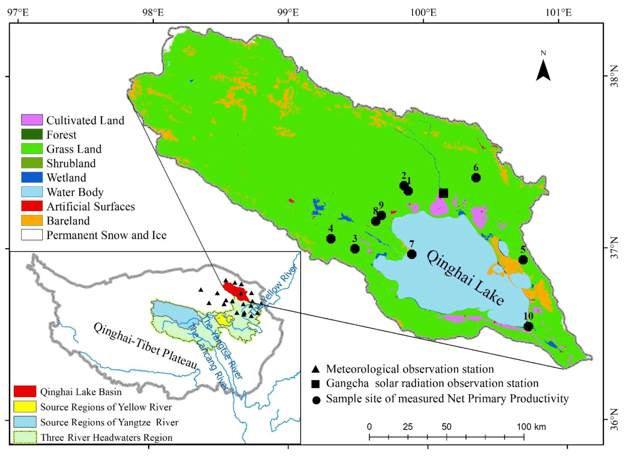
Figure 1 Location of the Qinghai Lake basin, with the sample and ground observation points shown. Note that the land cover is the GlobeLand30 product from 2020, which was obtained from http://www.globallandcover.com/ (last access: 30 January 2021).

2.2 Data sources

2.2.1 DEM

DEM data with a 90 m spatial resolution was derived from the Shuttle Radar Topography Mission (SRTM), as provided by the Geospatial Data Cloud (http://www.gscloud.cn/, last access: 25 December 2019). It was aggregated into a 500 m spatial resolution on the ArcGIS 10 software platform and then used to calculate SOL.

2.2.2 Solar radiation measurements

There is only one provincial ground solar radiation observation station in the study area. Observation data for the station in 2020 were not yet published at the time of this study, so we obtained its monthly SOL data for 2005, 2010, and 2015 from China Meteorological Data Service Centre (http://data.cma.cn/, last access: 10 June 2018) to verify the SOL simulation.

2.2.3 Ground meteorological data

The meteorological data of 20 ground observation stations in the study area and surrounding areas were obtained from China Meteorological Data Service Centre (http://data.cma.cn/, last access: 5 January 2021) and Qinghai Climate Center, Qinghai Province, China. The set contains the average monthly data for the years 2005, 2010, 2015, and 2020, including temperature (mean, minimum, and maximum), sunshine duration (only for 2020), sunshine percentage, precipitation, wind speed, and relative humidity and served to calculate traditional SOL, traditional WSC, and input parameters of the multisource-data-driven CASA model.

2.2.4 LUCC data

The GlobeLand30 product, at 30 m resolution in 2020, was obtained from http://www.globallandcover.com/ (last access: 30 January 2021) to identify grassland types and then determine its ε_max.

2.2.5 RS data

MODIS is a key sensor aboard the Terra and Aqua satellites. Terra MODIS and Aqua MODIS are covering the entire Earth's surface every 1 to 2 d. The Earth Science Data Systems Program generates 8 and 16 d, monthly, and other timescale-quality-controlled MODIS products. The products MOD11A2, MOD09A1, MOD13Q1, and MOD08M3 were obtained from the National Aeronautics and Space Administration (NASA; https://ladsweb.modaps.eosdis.nasa.gov/search/, last access: 6 January 2021). MOD13Q1, MOD09A1, and MOD11A2, with spatial resolutions ranging from 250 to 1000 m, were resampled to 500 m spatial resolution via the bilinear interpolation method. MOD08M3 was used to count the total cloud cover without unnecessarily adjusting its spatial resolution. In total, two images of 16 d products (MOD13Q1) and four images of 8 d products (MOD11A2 and MOD09A1) were averaged separately to calculate the monthly CASA parameters.

AMSR2 products, a surface SM dataset, have been evaluated in several previous studies and compared quite well with both observational and model simulation datasets from a variety of global test sites (Owe et al., 2008). We obtained the daily LPRM_AMSR2_DS_A_SOILM3 data of the AMSR2 products in July 2020 from the Goddard Distributed Active Archive Center (DAAC, https://disc.gsfc.nasa.gov/, last access: 11 October 2021) and averaged them to evaluate our WSC simulation results.

2.2.6 Field observation data

The field observation NPP data were surveyed via the quadrat method. Referencing the technical regulations for the survey and collection of the biomass of forest carbon pools (SACINFO, 2021) and the technical specification for field observations of a grassland ecosystem (Ministry of Ecology and Environment, PRC, 2021), three 1 m × 1 m quadrats were designed in the corner of square sample plots 25 m × 25 m in size. The average NPP values of these three quadrats was regarded as the NPP value of the sample plot. All aboveground vegetation in the quadrat was cut with scissors and placed into self-sealing bags and then placed into an oven at 105 ^∘C, baked for 15 min, and dried at 65 ^∘C until reaching a constant dry biomass value. The dry aboveground biomass (AGB) value was converted to NPP as follows (Zhang, 2016):

$$\begin{array}{}\text{(1)}& \mathrm{NPP}=\mathrm{AGB}\times C(\mathrm{1}+\mathrm{SR}),\end{array}$$

where C is carbon content coefficient converting biomass to NPP. It does not exceed 40 % for herbaceous plants in the Three River Headwaters region, QTP (Sun et al., 2017a), and was set to 37.13 % here according to the average carbon content of herbaceous plants (Zheng et al., 2007). SR represents the ratio of the aboveground biomass to the belowground biomass. Liu et al. (2020) reported that the average root–shoot ratio (the ratio of belowground and aboveground biomass) of alpine grassland is 6.87, so SR was set to $\mathrm{1.00}/\mathrm{6.87}$, i.e. SR equals 0.146 in this case.

From 23 July 2020 to 27 July 2020, we investigated a total of 30 quadrats and obtained 10 samples of NPP data to validate the RS-data-driven CASA model (Table 4).

3 Methods

3.1 CASA model

The CASA model incorporates meteorology, environment, and soil factors to simulate the physiological process of vegetation absorbing photosynthetically available radiation and transforming it into organic carbon. The model is as follows (Potter et al., 1993; Wang et al., 2017):

$$\begin{array}{}\text{(2)}& \begin{array}{rl}\mathrm{NPP}\left(x,t\right)& =\mathrm{0.5}\times \mathrm{SOL}(x,t)\times \mathrm{FPAR}(x,t)\times T_{\mathit{\epsilon }\mathrm{1}}\\ & \times T_{\mathit{\epsilon }\mathrm{2}}\times \mathrm{WSC}(x,t)\times {\mathit{\epsilon }}_{\max },\end{array}\end{array}$$

where NPP is the net primary production (g C m⁻² per month), 0.5 represents the proportion of the radiation which can absorbed by plants (0.4–0.7 µm​​​​​​​), SOL(x,t) is the total solar radiation incident on grid cell x in a given month (MJ m⁻² per month), FPAR(x,t) is the fraction of absorbed photosynthetically active radiation on grid cell x in a month, T_ε1 and T_ε2 are the temperature stress factors representing the effect of high and low temperature on light utilization efficiency, respectively, WSC(x,t) is the water stress coefficient on grid cell x in a month, and ε_max is the maximum possible efficiency (g C MJ⁻¹) under ideal conditions (no-stress temperature and no-stress water).

3.2 Improving CASA parameters with RS data

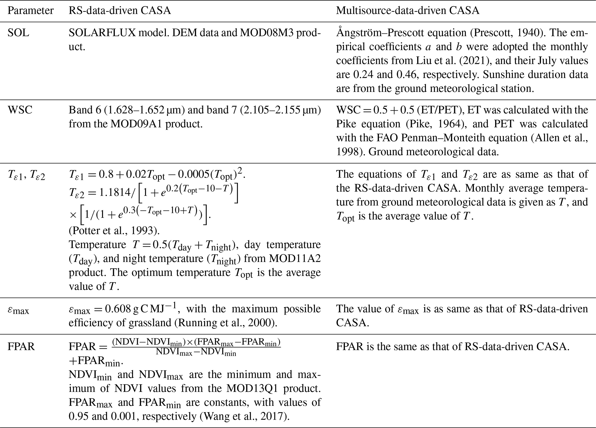
The RS data utilized here to improve CASA parameters are listed in Table 1. We focused specifically on improving the parameters of SOL and WSC.

Table 1 Calculation method and input data for CASA model parameters.

3.2.1 Calculation SOL by introducing RS total cloud cover

SOLARFLUX models (Hetrick et al., 1993; Kumar et al., 1997; Fu and Rich, 2002), which input DEM parameters and compute solar radiation over large areas, have been implemented for commercially available geographic information system (GIS) software such as ArcInfo (formerly ARC/INFO), ArcGIS, and Genasys. The solar radiation module of ArcGIS software takes into account the influence of atmospheric conditions, latitude, altitude, solar zenith angle and azimuth angle, terrain shade, slope, and aspect. The atmospheric conditions relevant to the present study were determined by the parameters diffuse_proportion and transmittivity. The diffuse_proportion is the fraction of global normal radiation flux that is diffused, which is expressed as a value from 0 to 1. Transmittivity, the fraction of radiation that passes through the atmosphere, ranges from 0 (no transmission) to 1 (all transmissions; ESRI, 2021).

There are distinct differences between diffuse_proportion and transmittivity on both clear and cloudy days (i.e. dependent on total cloud cover). The accurate determination of atmospheric conditions is the key to accurately estimating SOL. We introduced satellite total cloud cover to classify weather conditions and then determined the corresponding diffuse_proportion and transmittivity values. The total cloud cover data from the MOD08_M3 product, ranging from 0 (where the sky is completely clear) to 10 000 (where the sky is completely covered by clouds), was divided by 1000 to create 10 levels. For each level, the diffuse_proportion and transmittivity were determined according to a simple linear relationship (Table 2).

Table 2 Diffuse_proportion and transmittivity values under different total cloud cover levels.

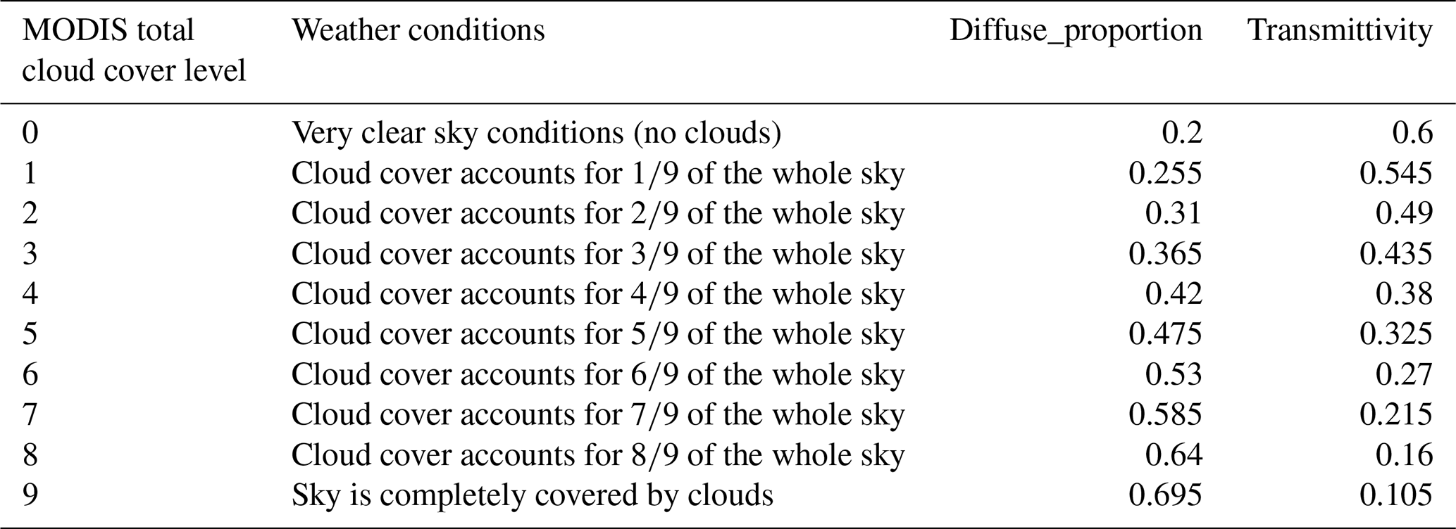
Note that, according to the scientific rule that diffuse_proportion has an inverse relation with transmittivity, the diffuse_proportion and transmittivity values were set to 0.2 and 0.6, respectively, in the case of very clear sky conditions. Under other cloud cover conditions, their values were determined according to a simple linear relationship, i.e. diffuse_proportion is 0.2 + 0.055level and transmittivity is 0.6−0.055​level. The step length of 0.055 was determined by repeatedly testing.

3.2.2 Improvement WSC using shortwave infrared reflectance

WSC reflects the effect of available water content on the solar radiation utilization efficiency of plants, ranging from 0.5 (extreme drought conditions) to 1.0 (extreme humidity). According to the relation that shortwave infrared reflectance is negatively correlated with the surface water content, scholars have proposed many water content RS indices. Referring to the form and connotation of the shortwave infrared soil moisture index (SIMI) proposed by Yao et al. (2011), we rewrote the WSC formula as follows:

$$\begin{array}{}\text{(3)}& {\displaystyle }\mathrm{WSC}=\mathrm{0.5}+\mathrm{0.5}(\mathrm{1}-N_{\mathrm{SIMI}}),\text{(4)}& {\displaystyle }{N}_{\mathrm{SIMI}}=(\mathrm{SIMI}-{\mathrm{SIMI}}_{\min })/({\mathrm{SIMI}}_{\max }-{\mathrm{SIMI}}_{\min }),\text{(5)}& {\displaystyle }\mathrm{SIMI}=\mathrm{0.7071}\sqrt{{\mathrm{SWIR}}_{\mathrm{1}}^{\mathrm{2}}+{\mathrm{SWIR}}_{\mathrm{2}}^{\mathrm{2}}},\end{array}$$

where WSC is the water stress coefficient, N_SIMI represents the normalized SIMI (ranging from 0 to 1), SIMI_max and SIMI_min are the maximum and minimum value of SIMI values, respectively, and SWIR₁ and SWIR₂ are the shortwave infrared reflectance, respectively.

4 Results

4.1 SOL

4.1.1 SOL simulated by the Ångström–Prescott equation

The SOL of ground stations was obtained using ground meteorological data and Ångström–Prescott equation (Table 1). The natural neighbour spatial interpolation approach was applied to convert the SOL of ground stations into grid SOL over study area (Fig. 2a).

Figure 2 Spatial distribution of the total solar radiation (SOL) in July 2020. (a) SOL simulated by the Ångström–Prescott equation. (b) SOL simulated by the improved approach.

4.1.2 SOL simulated by improved approach

The DEM, diffuse_proportion, and transmittivity determined by the MODIS total cloud cover were input into the Solar Radiation module of the ArcGIS10 software and then the SOL in July 2020 was simulated in the QLB (Fig. 2b). The simulated SOL ranged from 655.42 to 878.03 MJ m⁻² per month, with an average value of 738.80 MJ m⁻² per month. The surface of Qinghai Lake shows the lowest SOL of 695.50 MJ m⁻² per month. On the whole, SOL gradually increases along Qinghai Lake from southeast to northwest and is basically consistent with the actual total solar radiation.

4.1.3 Comparison of two SOL simulation approaches

We analysed the accuracy of simulation SOL from the Ångström–Prescott equation and improved the SOL approach with the measured SOL monthly data in 2005, 2010, and 2015 (at present, only the measured SOL data in these periods could be collected for the purposes of this study; Table 3). The root mean square error (RMSE) of the Ångström–Prescott equation and our improved approach, respectively, are 162.24 and 95.38 MJ m⁻² per month. Correspondingly, the mean absolute percent errors (MAPEs) of the two approaches are 24.56 % and 17.78 %, the July root mean square errors (RSMEs) are 274.34 and 70.66 MJ m⁻² per month, and the July MAPEs are 39.53 % and 9.25 %, respectively. To simulate SOL, the improved approach significantly increased the accuracy in the study area.

Table 3 Measured versus simulated SOL.

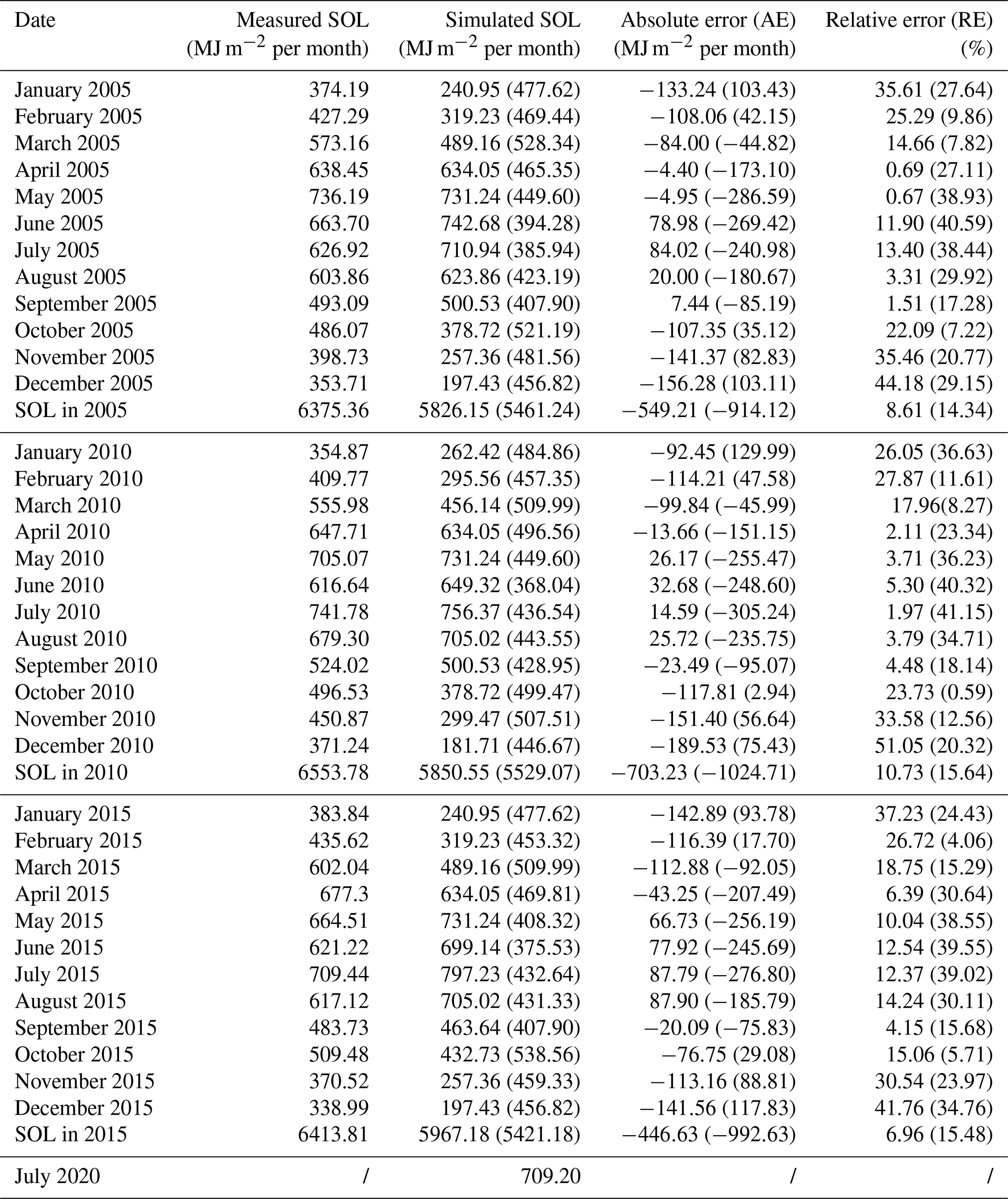
Note that the values in parentheses are the values of SOL simulated by the Ångström–Prescott equation and the corresponding error values.

4.2 WSC

4.2.1 Traditional WSC

The WSC of the ground stations was obtained using ground meteorological data for July 2020 and the approaches listed in Table 1. The natural neighbour approach was used to convert the WSC of ground stations into grid WSC over study area (Fig. 3a).

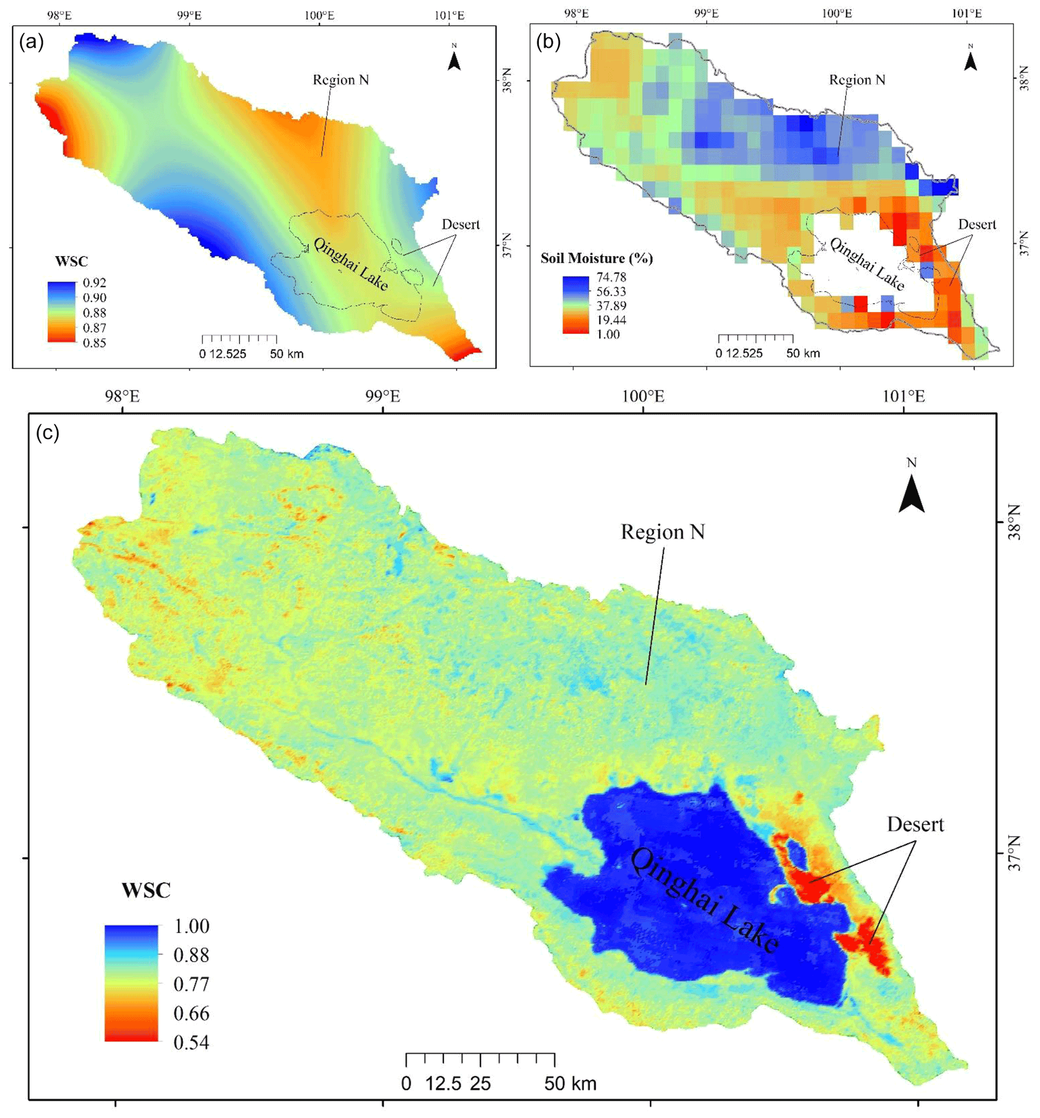
Figure 3 Spatial distribution of the water stress coefficient (WSC) in July 2020. (a) WSC simulated by the traditional method. (b) Surface soil moisture of the AMSR2 products. (c) WSC calculated with the RS shortwave infrared band.

4.2.2 Improved WSC

Using the shortwave infrared reflectance of bands 6 and 7 from MOD09A1, we applied Eqs. (3)–(5) and obtained the WSC in July 2020 (Fig. 3c). The WSC values were relatively high (>0.86) around Qinghai Lake and in river valleys and in the river source areas at higher altitudes, which indicates that these places have sufficient water supply. The desert ecosystem in the east of the Qinghai Lake showed the lowest WSC (0.54–0.68), which indicates that the ecosystem has insufficient water supply.

4.2.3 Comparison of two WSC simulation approaches

WSC, a measure of the availability of water to plants, essentially reflects the impact of the environmental water content on plants. For a grassland ecosystem, to a certain extent, surface SM can indirectly reflect the environmental water content. As a general rule, a higher value of WSC indicates a higher environmental water content. The surface SM dataset (LPRM_AMSR2_DS_A_SOILM3) was used to evaluate the WSC results simulated by different approaches.

The SM is high in north of Qinghai Lake (region N), and it is the lowest in the desert ecosystem (Fig. 3b). In region N, the traditional WSC shows low values, which indicates that the environmental water content is low, and the desert ecosystem showed a lower values but not the lowest. Hence, the traditional WSC results are inconsistent with surface SM; they cannot reflect the spatial distribution of environmental water content accurately. The sparse distribution of ground meteorological stations caused uncertainty in the interpolation results.

The improved WSC results compared well with the surface SM in above two regions. Their spatial distribution are approximately consistent with the actual water contents in study area, so it is feasible to estimate WSC using RS shortwave infrared reflectance.

4.3 NPP

4.3.1 Comparison of multisource and RS-data-driven CASA

The measured NPP obtained in July 2020 was used to verify the accuracy of the multisource- and RS-data-driven CASA models (Table 4). For the NPP simulated by multisource-data-driven CASA (Fig. 4a), the relative error (RE) ranges from 20.20 % to 68.43 %, the MAPE is 44.80 %, the absolute error (AE) ranges from −112.88 to −16.01 g C m⁻² per month, and the RMSE is 57.43 g C m⁻² per month. For the NPP simulated by RS-data-driven CASA, the RE ranges from 2.49 % to 47.80 %, the MAPE is 22.14 %, the AE ranges from −34.54 to 46.90 g C m⁻² per month, and the RMSE is 26.36 g C m⁻² per month. The simulation results of RS-data-driven CASA are more in accordance with the measured NPP, and RS-data-driven CASA significantly increased the accuracy of grassland NPP in the study area.

Table 4 Measured versus simulated NPP.

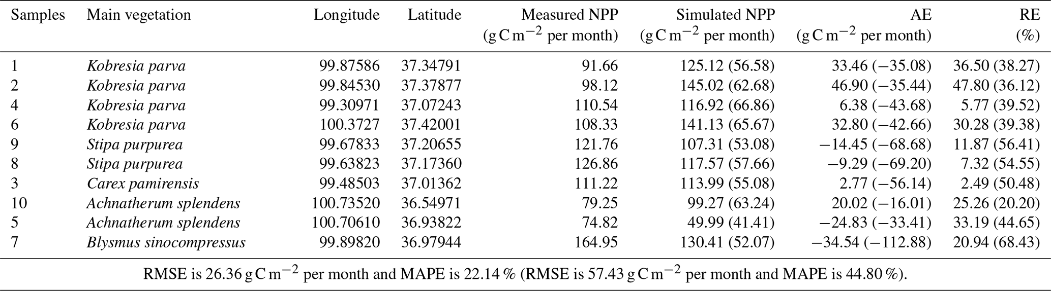
Note that the values in parentheses are the values of NPP simulated by multisource-data-driven CASA and the corresponding error values.

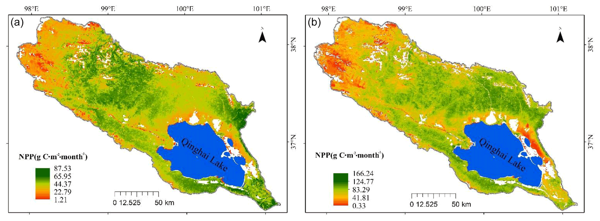
Figure 4 Spatial distribution of grassland net primary productivity (NPP) in July 2020. (a) NPP simulated by multisource-data-driven CASA. (b) NPP simulated by RS-data-driven CASA.

4.3.2 NPP spatial distribution

The values of NPP simulated by RS-data-driven CASA are lower in the northwestern parts of the basin and east of Qinghai Lake than elsewhere in the study area (Fig. 4b). The main vegetation in the northwest is alpine Kobresia humilis meadow plants, such as Saussurea pumila and Saussurea alpina, which have low vegetation productivity and NPP values ranging from 0.33 to 87.52 g C m⁻² per month. The main vegetation in the southwestern coast of Qinghai Lake and the middle part of the basin is Stipa purpurea Griseb. and Carex infuscata Nees alpine grasslands, which have higher vegetation productivity and NPP values greater than 87.52 g C m⁻² per month. NPP appears to decrease from the southeast to northwest, which is consistent with the distribution patterns of vegetation type.

5 Discussion and recommendations

5.1 SOL

Various approaches for simulation SOL consider the atmospheric effects on solar radiation from different perspectives. The Ångström–Prescott equation uses the sunshine duration (or sunshine percentage) to quantify atmospheric effects on solar radiation. We use the parameters of diffuse_proportion and transmittivity determined by total cloud cover to quantify these effects. The total cloud cover determines the weather conditions and affects the atmospheric conditions. Total cloud cover information can be used to directly determine weather conditions and indirectly determine atmospheric conditions. In this study, weather conditions were classified into 10 levels according to the satellite total cloud cover. The two important parameters of the SOLARFLUX model, diffuse_proportion and transmittivity, were determined for each level on the basis of a linear relationship. The atmospheric conditions could be further divided into 100 or more refined levels to determine the values of diffuse_proportion and transmittivity under different cloud cover conditions to improve the SOL simulation accuracy.

It is important to note that the SOLARFLUX model is designed only for local landscapes/regional scales, so it is generally acceptable to use one latitude value for the whole DEM. It is necessary to divide larger areas into zones of varying latitude as the latitudes exceed 1^∘ (ESRI, 2021).

5.2 WSC

The environmental water content can regulate vegetation NPP by affecting the photosynthetic capacity of plants. The WSC reflects the influence of environmental water content on vegetation NPP. The traditional WSC simulation approach applies a ratio of ET to PET to measure the availability of the environmental water content. ET and PET can be obtained by different approaches and data sources, resulting in substantial differences in ET and PET even if the same data are used, thus creating differences in WSC. The WSC result of our improved approach is certain as long as the same RS data are input in Eqs. (3)–(5). In addition, the proposed WSC approach has the RS retrieval mechanism of environmental water content. Soil and vegetation water contents are closely related to their shortwave infrared spectral reflectance; small changes in these contents can cause substantial changes in shortwave infrared spectral reflectance. Thus, the RS shortwave infrared band is sensitive to the environmental water content and can be used to calculate WSC. Many satellite sensors have shortwave infrared bands, such as MODIS (1.628–1.652 µm; 2.105-2.155 µm), LandSat 8 (1.560–1.660 µm; 2.100–2.300 µm), Sentinel-2 (1.565–1.655 µm; 2.100–2.280 µm), and HJ-1A and HJ-1B (1.550–1.750 µm). Scholars have developed many RS water content indexes such as SIMI, MSIWSI (Dong et al., 2015), and SWCI (Du et al., 2007). We modified the WSC using SIMI and the two shortwave infrared bands of MODIS in this study. The shortwave infrared bands of satellite sensors mentioned above, and the MSIWSI, SWCI, or other RS water content indices, can also be considered to calculate WSC.

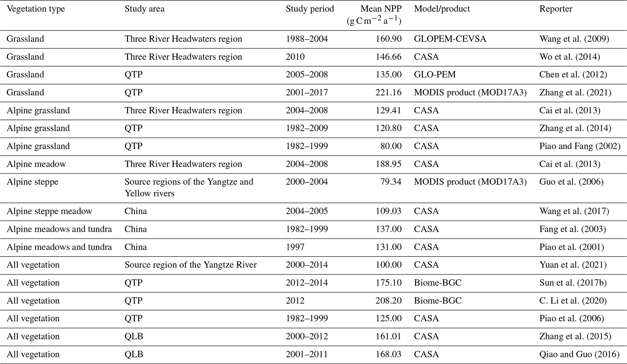
5.3 Rationality of NPP simulation results

We compared our simulated NPP with previously published results (Table 5). Our simulated grassland NPP in July 2020 has an average value of 108.01 ± 26.31 g C m⁻² per month, which is similar to most published results but smaller than some of them. The QLB is located on the QTP, which has a severely cold climate and a short growing season. Vegetation is in its growth stage in July, and its biomass reaches the highest values for the whole year before the end of August or the beginning of September, which means that grassland NPP also reaches the annual maximum value about a month later. The reported NPP encompasses the full year, so it is reasonable that July NPP simulation values would be lower than some previously reported NPP values.

Table 5 Published versus simulated NPP.

The simulation NPP values of Kobresia parva and Stipa purpurea are larger and smaller, respectively, than the measured NPP values. Kobresia parva is distributed in high-altitude areas which herders often utilize as summer pastures. Grazing cattle and sheep reduces the biomass of these areas, resulting in lower measured NPP values. Kobresia parva is characterized by low and short (1–3 cm) vegetation, with densely clumped stems and high coverage. Grazing livestock does not significantly affect its reflectance at red and near-infrared bands. For grazed and ungrazed Kobresia parva, the NDVI calculated by the reflectance of red and near-infrared bands is almost the same; the FPAR values calculated by NDVI are also very similar, so the simulated NPP values are nearly identical as well. Due to the lower measured NPP value of Kobresia parva caused by grazing, the NPP simulation values of Kobresia parva appear to be relatively high. Stipa purpurea, distributed in low-altitude areas that herders often use as winter pastures, is an ideal vegetation type to verify the NPP model as it is not consumed by cattle, sheep, or other livestock during the summer. Stipa purpurea has a thin stalk up to 45 cm high, and its leaf curls into needles with a strongly lignified epidermis and purple spikelets. These characteristics result in a lower reflectance at red and near-infrared bands, which leads to lower NDVI and FPAR values. Thus, the simulated NPP values of Stipa purpurea are relatively low.

5.4 Uncertainty

According to Eq. (1), the uncertainty of measured NPP originates from uncertainties in AGB, C​​​​​​​, and SR. There is randomness in which three quadrats are selected from the four corners of square sample plot, resulting in uncertainty in the AGB collection. In our case, C and SR are adopted as the values reported in the literature rather than measured values, which inevitably cause errors.

The uncertainty of multisource-data-driven CASA and its parameters is mainly caused by spatial interpolation methods. The WSC interpolation resulting from spline and kriging methods have significantly different values and spatial patterns (Fig. 5). Sample 7 (see Table 4) has the maximum errors of the estimation NPP. Its SOL, simulated by traditional approach, is 271.39 MJ m⁻² per month, which is obtained by interpolating the SOL of observation stations. The average simulated and measured SOL of the Gangcha observation station is 434.59 and 692.71 MJ m⁻² per month, respectively (Table 3). The distance from this station to sample 7 is about 43 km. Hence, for sample 7, the errors of multisource-data-driven CASA are mainly caused by the parameter SOL and the spatial interpolation method.

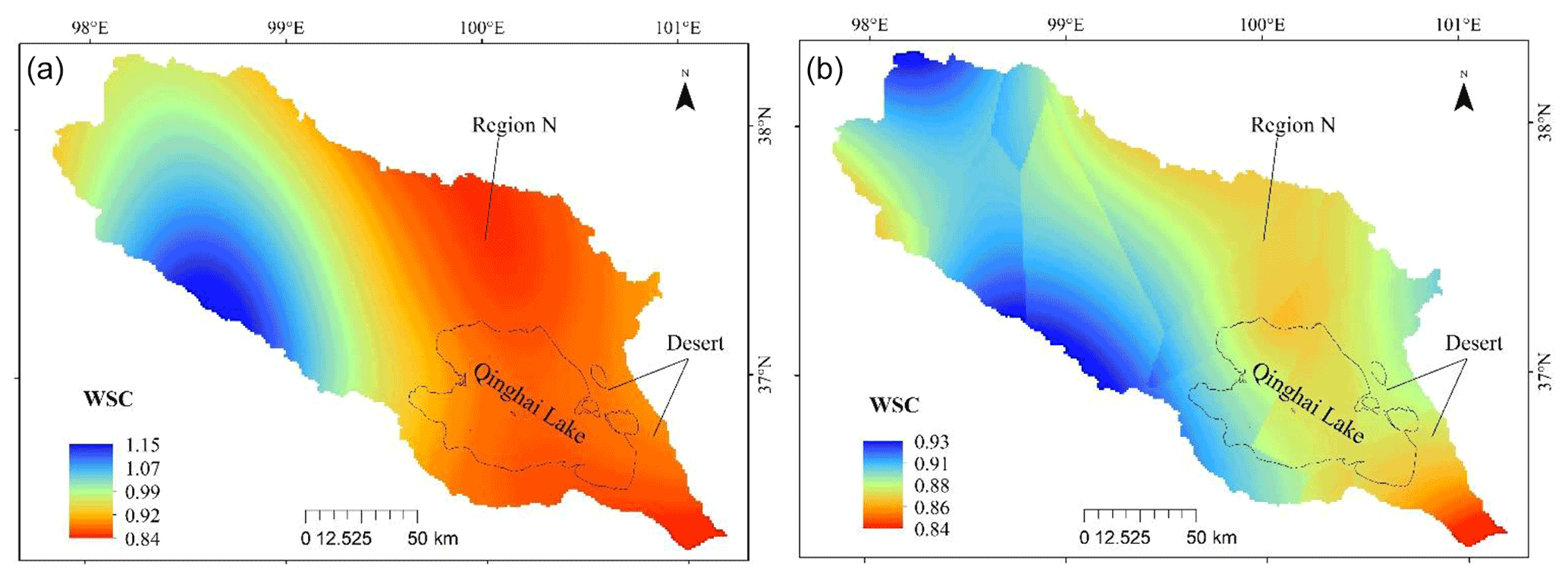
Figure 5 Comparison map of water stress coefficient (WSC) interpolation results in July 2020. (a) WSC from the spline method. (b) WSC from the kriging method.

The uncertainty of RS-data-driven CASA mainly stems from the RS product data quality and uncertainty propagation across parameters. The RS products usually have corresponding data quality assurance describing the uncertainty of each pixel (e.g. the uncertainty of production MOD11A2; details regarding quality assurance can be found online at https://icess.eri.ucsb.edu/modis/LstUsrGuide/usrguide_index.html, last access: 8 May 2021). The combined uncertainty of simulation NPP is determined by the uncertainty propagation from parameters. In our case, the combined uncertainty of grassland NPP is 108.01 ± 26.31 g C m⁻² per month. The uncertainty contribution of alpine meadow and other grassland types, and uncertainty propagation and quantification, will be carried out systematically in future work.

6 Conclusions

The traditional CASA model, driven by multisource data such as meteorology, soil, and RS, has notable disadvantages. In this study, we attempted to drive a CASA entirely by RS data. We conducted a case study of alpine grasslands in the QLB to find that it is feasible to calculate the CASA parameters of SOL, WSC, T_ε1, and T_ε2 using RS data. The estimated NPP results were reliable. The main conclusions of this work can be summarized as follows.

• Cloud cover was used to quantify the atmospheric effects on solar radiation. It is only necessary to use DEM and RS total cloud cover data to simulate SOL. The improved SOL simulation approach has a monthly RMSE and MAPE of 95.38 MJ m⁻² per month and 17.78 %, respectively.

• According to the RS retrieval mechanism of the environmental water content, shortwave infrared reflectance was used to modify the WSC. The improved WSC simulation approach simplified the input parameters. Its results are more consistent with the actual environment water contents than that of the traditional WSC in the study area.

• The RS-data-driven CASA, without the support of ground observation data (e.g. soil or meteorology), yields simulations in closer accordance with measured NPP values. The RE ranges from 2.49 % to 47.80 %, the MAPE is 22.14 %, the AE ranges from −34.54 to 46.90 g C m⁻² per month, and the RMSE is 26.36 g C m⁻² per month. The simulated NPP values of Kobresia parva in the grazing area and Stipa purpurea are higher than and lower than the respective real values. The combined uncertainty of grassland NPP is 108.01 ± 26.31 g C m⁻² per month. The uncertainty propagation and quantification will be the focus of our future work.