the Creative Commons Attribution 4.0 License.
the Creative Commons Attribution 4.0 License.
 | 09 Sep 2022
The bulk parameterizations of turbulent air–sea fluxes in NEMO4: the origin of sea surface temperature differences in a global model study
Doroteaciro Iovino
Laurent Brodeau
Simona Masina
Wind stress and turbulent heat fluxes are the major driving forces that modify the ocean dynamics and thermodynamics. In the Nucleus for European Modelling of the Ocean (NEMO) ocean general circulation model, these turbulent air–sea fluxes (TASFs) can critically impact the simulated ocean characteristics. This paper investigates how the various bulk parameterizations used to calculate turbulent air-sea fluxes in NEMOv4 can lead to substantial differences in the estimation of sea surface temperatures (SSTs). Specifically, we study the contributions of different aspects and assumptions of the bulk parameterizations in driving the SST differences in the NEMO global model configuration at ∘ of horizontal resolution. These aspects include the use of the skin temperature instead of the bulk SST in the computation of turbulent heat flux components and the estimation of wind stress and turbulent heat flux components, which vary in each parameterization due to different bulk transfer coefficients. The analysis of a set of short-term sensitivity experiments where the only change is related to one of the aspects of the bulk parameterizations shows that parameterization-related SST differences are primarily sensitive to wind stress differences and to the implementation of skin temperature in the computation of turbulent heat flux components. In addition, in order to highlight the role of SST–turbulent heat flux negative feedback at play in ocean simulations, we compare the TASF differences obtained using the NEMO ocean model with the estimations by Brodeau et al. (2017), who compared the different bulk parameterizations using prescribed SSTs. Our estimations of turbulent heat flux differences between bulk parameterizations are weaker than those found by Brodeau et al. (2017).
- Article
(26537 KB) - Full-text XML
-
Supplement
(11438 KB) - BibTeX
- EndNote


Ocean and atmosphere circulations are highly influenced by the transfer of momentum and heat at the air–sea interface (e.g., Gill, 1982; Siedler et al., 2013). These transfers of energy are primarily driven by surface radiative flux and turbulent air–sea fluxes (TASFs), which include wind stress and turbulent heat flux components (THFs, latent and sensible heat fluxes). In the upper ocean, wind stress is a major driving force of basin-scale circulation (e.g., Chen et al., 1994; Shriver and Hurlburt, 1997), and THFs are important for determining its thermal properties (e.g., Yuen et al., 1992; Swenson and Hansen, 1999). Therefore, both wind stress and THFs are important for the evolution of the sea surface temperature (SST) because of their contribution to turbulent mixing within the ocean surface mixed layer (e.g., Barnier, 1998).
Since direct observations of TASFs are sparse in space and time, the estimates are derived using bulk formulas, which relate each component of the turbulent air–sea flux to more easily measurable and widely available meteorological surface atmospheric variables (e.g., wind speed, air temperature, air specific humidity) through bulk transfer coefficients. These coefficients are estimated using bulk parameterizations. Different bulk parameterizations are currently used, which are traditionally developed statistically, comparing in situ meteorological observations of surface atmospheric variables with TASFs derived from ship and buoy measurements (Large and Pond, 1981, 1982; Smith, 1988; Fairall et al., 1996, 2003; Bradley and Fairall, 2007; Edson et al., 2013).
In the NEMO ocean general circulation model (OGCM), TASFs are computed by means of bulk formulas using prescribed surface atmospheric variables (air temperature, air humidity, wind) and the prognostic SST of the model (hereinafter the “online prognostic SST approach”). This approach incorporates the response of the ocean (i.e., SST) to atmospheric events into the estimation of the THFs and of long-wave radiation (i.e., non-solar-heat-flux components, NSHFs) at each time step of the numerical experiment. The feedback between the ocean and the atmosphere partially simulates the energy exchange between them (Kara et al., 2000). The OGCM entails the selection of a given bulk parameterization, which influences the magnitude of the wind stress and the THFs (Kara et al., 2000). The TASFs affect the simulated ocean characteristics and in particular the evolution of the SST (Torres et al., 2019). The online prognostic approach only partially closes the air–sea feedback. Surface winds and clouds are affected by the SST structure on daily timescales which, in turn, affect the SST and the TASFs (Desbiolles et al., 2021; de Szoeke et al., 2021; Gaube et al., 2019; Li and Carbone, 2012; Small et al., 2008). The closed air–sea feedback (hereinafter the “coupled approach”) in the system could substantially impact the turbulent fluxes (Lemarié et al., 2021; Small et al., 2008); however, the coupled approach is not yet mature in the ocean model community. Recently, Lemarié et al. (2021) exploited a simplified atmospheric boundary layer model (ABL) to improve the representation of air–sea interactions in NEMOv4.2. However, the online prognostic SST approach is still widely used by the ocean modeling community in a variety of applications.
Brodeau et al. (2017) compared a set of bulk parameterizations which compute TASFs using the prescribed SST (hereinafter “the offline prescribed SST approach”) rather than the prognostic SST of the model. They reported that the use of different bulk parameterizations to estimate TASFs can typically produce differences in total turbulent heat flux (QT, i.e., the sum of the THFs and the latent and sensible heat fluxes) of about 10 W m−2 and differences in wind stress of about 20 mN m−2. The online prognostic SST approach, used in the NEMO experiments performed in our study, can substantially modify these estimates through the negative SST feedback on QT, which likely dampens the QT discrepancies across the various bulk parameterizations (Seager et al., 1995).
The aim of this work is to better understand the response of the prognostic SST to the TASFs and to their parameterization in NEMO version 4.0 at ∘ of horizontal resolution. We also discuss the role of the SST–QT negative feedback at play in the online prognostic SST approach.
We address the sensitivity of the SST to various aspects of the different bulk parameterizations, such as the inclusion of the skin temperature in the computation of the THFs and the role of bulk transfer coefficients in the estimation of the wind stress and THFs. We thus analyzed differences between short-term sensitivity experiments where bulk assumptions are excluded (e.g., skin temperature) or where bulk transfer coefficients are computed by mixing the different bulk parameterizations. Lastly, in order to highlight the role of the SST–QT negative feedback at play in our online prognostic SST approach, we compare TASFs with the estimations from Brodeau et al. (2017). We also provide a simple validation of the various experiments against an SST observed data set; however, the main objective of the work was to investigate the impact of a set of bulk parameterizations on the SST generated by NEMO rather than evaluating their accuracy in reproducing it.
This paper is organized as follows. Section 2 presents the model used for this study, a short overview of the bulk formulas implemented in NEMOv4, the experimental setup, and the modifications introduced in the bulk parameterizations used for the sensitivity experiments. In Sect. 3, we present the parameterization-related SST discrepancies, quantify SST discrepancies related to various aspects of the different bulk parameterizations, and discuss our findings and compare them with the literature. Our conclusions are drawn in Sect. 4.
2.1 NEMOv4 model configuration
The sensitivity of the prognostic SST to bulk parameterizations is investigated in a numerical study using the Nucleus for European Modelling of the Ocean (https://www.nemo-ocean.eu/, last access: 31 August 2022) (NEMO, version 4.0, revision 12957). NEMO is a three-dimensional, free-surface, hydrostatic, primitive-equation global ocean general circulation model (Madec and the NEMO System Team, 2019) coupled to the Sea Ice modelling Integrated Initiative (SI3, NEMO Sea Ice Working Group, 2019). Our configuration uses the global ORCA025 tripolar grid (Madec and Imbard, 1996) with ∘ horizontal resolution (27.75 km) at the Equator, which increases with latitude, e.g., it is 14 km at 60∘. The vertical grid has 75 levels whose spacing increases with a double hyperbolic tangent function of depth from 1 m near the surface to 200 m at the bottom, with partial steps representing the topography of the bottom (Barnier et al., 2006). The bathymetry of the model is based on the combination of the ETOPO1 data set (Amante and Eakins, 2009) in the open ocean and GEBCO (IOC and IHO, 2003) in coastal regions. The horizontal turbulent viscosity is parameterized by means of a biharmonic function with a value of 1.8×10¹¹ m4 s−1 at the Equator, reducing poleward as the cube of the maximum grid cell size. The advection of the tracers uses a total variance dissipation (TVD) scheme (Zalesak, 1979). The Laplacian lateral tracer mixing is along isoneutral surfaces with a coefficient of 300 m2 s−1. The vertical mixing of tracers and momentum is parameterized using the turbulent kinetic energy (TKE) scheme (Blanke and Delecluse, 1993). Subgrid-scale vertical mixing processes are represented by a background vertical eddy diffusivity of m2 s−1 and a globally constant background viscosity of m2 s−1. The friction at the bottom is quadratic, and a diffusive bottom boundary layer scheme is included. The continental runoff data are a monthly climatology derived from the global river flow and continental discharge data set for the major rivers (Dai and Trenberth, 2002; Dai et al., 2009) and estimates by Jacobs et al. (1996) for the Antarctic coastal freshwater discharge. The initial conditions for temperature and salinity are provided by the World Ocean Atlas 2013 (Levitus et al., 2013). All the experiments are forced with the hourly ERA5 reanalysis of the ECMWF (Hersbach et al., 2020).
2.2 The bulk formulas and their parameterization in NEMO4.0
As stated in the “Introduction”, NEMO uses the online prognostic SST approach to compute TASFs, which are estimated using the prognostic SST and prescribed atmospheric surface variables by means of aerodynamic bulk formulas:
where τ is the wind stress, QH is the turbulent flux of sensible heat, E is the evaporation, and QL is the turbulent flux of latent heat. Throughout this paper, we use the convention that a positive sign of τ, of THFs (QH and QL), and of the total turbulent heat flux QT (QT = QH+QL) means a gain in the relevant quantity for the ocean. The term ρ is the density of air; Cp is the heat capacity of moist air, and Lv is the latent heat of vaporization. uz is the wind speed vector at height z, which may be absolute or relative to the ocean currents. The bulk scalar wind speed U is the scalar wind speed with the potential inclusion of gustiness. Convective gustiness is a temporary increase in the wind speed due to friction and free convection, and is active and significant in very calm wind conditions with an unstable near-surface atmosphere. It is added to the wind speed and avoids the zero wind singularity. θz and qz are the potential temperature and specific humidity of air at height z, while Ts and q0 are the potential temperature and specific humidity at the surface. Depending on the bulk parameterization used, Ts can be the temperature at the air–sea interface (the sea surface skin temperature, hereinafter “SSTskin”) or typically at a depth of 1 m (the bulk sea surface temperature, SST). The SSTskin differs from the SST due to two effects with opposite signs: the cool skin and warm layer (CSWL). The cool skin is the cooling of the millimeter-scale uppermost layer of the ocean, which ensures a steep vertical gradient of temperature that sustains the heat flux continuity between the ocean and atmosphere. The warm layer is the warming of the upper few meters of the ocean in daytime and sunny conditions.
CD, CH, and CE are the bulk transfer coefficients (BTCs) for wind stress, sensible heat, and moisture, respectively.
The main differences between bulk parameterizations are therefore usually related to:
-
The use of the skin temperature (SSTskin) rather than the bulk SST in the estimation of near-surface atmospheric stability and the bulk formulas
-
The dependence of the exchange coefficients on the wind speed
-
The inclusion of convective gustiness in the wind calculation
-
The effect of including ocean currents in the wind stress.
In this study, we disentangle the effects of the first two aspects on the SST (Sects. 3.2, 3.3, and 3.4) and discuss the effect of the inclusion of convective gustiness in the wind stress computation (Sect. 3.4). The effects of the ocean current interaction/feedback in the bulk formulation have been widely explored (e.g., Renault et al., 2019a, b; Sun et al., 2019). Although many studies have highlighted the substantial difference in the surface input to the ocean between calculations that use absolute vs. relative wind, we decided to leave this aspect to future work, since the implementation of this correction essentially depends on the characteristics of the forcing fields (Renault et al., 2020).
The online prognostic SST approach of NEMO uses the modeled SST at each time step to estimate NSHFs (i.e., THFs + long-wave radiation). In our experiments, we only focus on the NSHFs computed by bulk formulas, namely the THFs. The SST responds to the total turbulent heat flux QT at each time step: the QT generate SST anomalies, and SST anomalies, in turn, modulate QT. Specifically, the SST and QT feed back negatively: when the SST becomes anomalously cold, QT increases, which increases the SST. Then QT will decrease, and so on. This negative feedback of the online prognostic SST reduces the differences in heat fluxes across the different bulk parameterizations. On the other hand, the wind stress is not affected by this type of first-order feedback at play for the QT.
In this study, we focus on three bulk parameterizations implemented in NEMOv4: NCAR (Large and Yeager, 2009), COARE 3.6 (Edson et al., 2013; Chris Fairall, private communication, 2016 hereinafter “COARE”), and ECMWF as coded in the Aereobulk package (Brodeau et al., 2017). All the codes used to estimate TASFs in the NEMOv4.0 framework originate from this AeroBulk package (Brodeau et al., 2017). COARE and ECMWF parameterizations are designed to be used with the SSTskin, so the two algorithms include a CSWL parameterization to estimate it. NCAR uses the bulk SST in the heat flux calculation, and the zero-wind singularity is avoided by simply setting a minimum value for the scalar wind speed of 0.5 m s−1. To calculate the BTCs, the bulk parameterizations rely on an empirical closure. More specifically, in COARE and ECMWF parameterizations, the computation of BTCs uses the Monin–Obukhov similarity theory (MOST, Monin and Obukhov, 1954). As such, BTCs are a function of the roughness lengths and of the stability of the atmospheric surface layer. The NCAR parameterization uses a combination of the MOST theory with a semi-empirical form of the drag coefficient in which the BTCs are computed as a function of neutral wind speed (e.g., the wind speed in neutral stability conditions and at 10 m reference level, UN10). The BTCs are shifted to the current atmospheric stability.
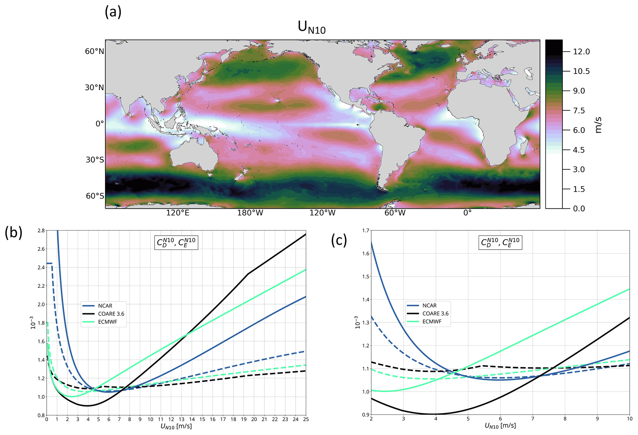
Figure 1(a) Annual mean UN10 from NCAR parameterization. (b) Neutral drag and moisture transfer coefficients ( and ) for COARE (black), NCAR (blue), and ECMWF (green) bulk parameterizations (solid and dashed lines, respectively) as functions of the neutral wind speed at 10 m. (c) Zoom of panel (b) for the wind range 2–10 m s−1.
Figure 1 shows the UN10 annual mean and the neutral BTCs as a function of UN10 for the selected bulk formula parameterizations. Due to the stronger neutral drag coefficient , the NCAR parameterization tends to enhance wind stress with respect to COARE and to ECMWF under light wind conditions (u<5 m s−1). On the other hand, the ECMWF parameterization enhances wind stress with respect to NCAR and COARE for wind speeds above 5 m s−1, while COARE enhances it for wind speeds above 13 m s−1. Under weak-wind conditions, the NCAR parameterization tends to enhance evaporation with respect to COARE and ECMWF due to the stronger (see Fig. 1). For a detailed explanation of the BTC derivation for each bulk parameterization, please refer to the technical report by Bonino et al. (2020).
2.3 Experimental setup
In order to investigate the roles of different aspects of bulk parameterizations in driving the prognostic SST, we performed six numerical experiments (Table 1). All the experiments lasted 1 year, starting from January 2016 after a 1 year spin-up. There was no intent to analyze this year in relation to a specific climatic mode. The simulations were forced by the hourly surface atmospheric variables of the ERA5 reanalysis (Hersbach et al., 2020).
We first performed three experiments (hereinafter “control experiments”) in order to quantify the bulk parameterization-related SST discrepancies. In particular, we performed ECMWF_S, COARE_S, and NCAR experiments, which used the ECMWF, COARE, and NCAR parameterizations, respectively. The ECMWF_S and COARE_S experiments used the SSTskin (through their respective CSWL schemes) and considered convective gustiness in the wind speed calculation. In contrast, the NCAR experiment computed THFs using the bulk SST, and the convective gustiness was not considered in the wind speed computation.
In order to disentangle the contribution of the skin temperature and the contribution of the different wind stresses and THFs in driving sea surface temperature differences, we performed three sensitivity experiments (hereinafter “mixed experiments”). First, we performed the ECMWF_NS experiment, which uses the ECMWF parameterization, and THFs were computed using the bulk SST rather than the SSTskin. Second, we performed the CdNC_CeEC_NS experiment, which used the ECMWF parameterization to calculate CH and CE BTCs and the NCAR bulk formula to calculate CD BTC. THFs were computed using the bulk SST.
We also performed an additional experiment, called ECMWF_NS_NG, which differed from ECMWF_NS only in terms of the exclusion of the convective gustiness from the wind speed calculation. We used the absolute wind, which means that the parameterizations did not include the ocean current feedback to calculate the wind in Eq. (1a).
Here we discuss the parameterization-related discrepancies in the control experiments in terms of TASFs (i.e., QT and τ), wind stress curl (WSC), SST, and meridional heat transport (Sect. 3.1). Then, we try to analyze the contributions of various aspects of the parameterizations in driving these SST and meridional transport discrepancies. In particular, the comparison between ECMWF_S and ECMWF_NS is used to determine the skin temperature contribution (Sect. 3.2), while the comparisons between CdNC_CeEC_NS and NCAR (Sect. 3.3) and between CdNC_CeEC_NS and ECMWF_NS (Sect. 3.4) teach us about the contribution of the bulk transfer coefficients. In Sect. 3.4, we also compare ECMWF_NS_NG and ECMWF_NS experiments to show the effect of the inclusion of convective gustiness in the wind speed calculation on wind stress computation (shown in the Supplement). For each pair of experiments, we only show the differences in TASFs and their components (e.g., U, CD, CE) which are relevant to understanding the SST or meridional heat transport discrepancies. The complementary TASF differences are reported in the Supplement. We analyze annual mean differences between experiments and assess their statistical significance using the t-test.
3.1 Parameterization-related discrepancies
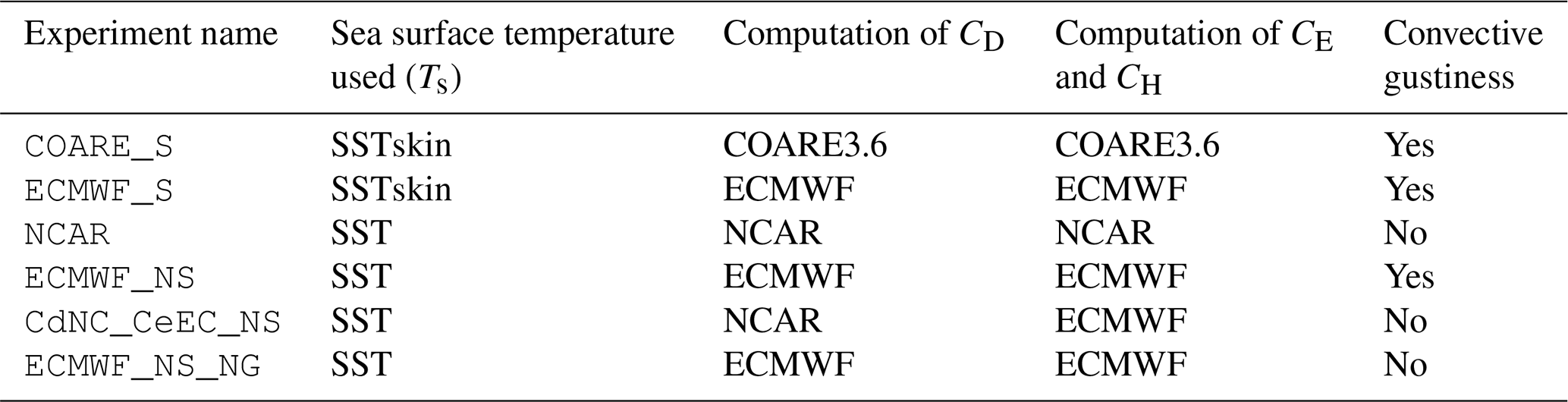
We compared the SSTs simulated by the ECMWF_S, COARE_S, and NCAR control experiments with the European Space Agency (ESA) Climate Change Initiative (CCI) SST data set v2.0 (hereinafter “ESA CCI SST data set”), which consists of daily-averaged global maps of SST on a 0.05∘ × 0.05∘ regular grid covering the period from September 1981 to December 2016 (Merchant et al., 2019).
All the control experiments present a warm bias in the eastern Pacific, in the eastern boundary upwelling systems (EBUS), in the western boundary currents (WBCs) and in the Antarctic Circumpolar Current (ACC) region. The SST reproduced by COARE_S and ECMWF_S shows a cold bias of about −1 ∘C in the North Atlantic open ocean at mid-latitudes and a warm bias of about 0.5 ∘C in the Indian Ocean and the western Pacific (Fig. 2a, b). The NCAR SST is also colder than observations, with a larger bias of about −2 ∘C in the North Atlantic (Fig. 2c). The bias is generally higher compared with the other two experiments and covers wider areas.
Figure 3 shows the differences in total turbulent heat fluxes, wind stress, and wind stress curl from ECMWF_S and COARE_S with respect to NCAR. The ECMWF_S wind stress is slightly weaker with respect to NCAR over the equatorial band and stronger elsewhere (Fig. 3a). In terms of wind stress, COARE_S is weaker than tNCAR over a broader region with respect to ECMWF_S, namely over the areas characterized by calm wind conditions (see Fig. 1). The WSC patterns are similar for the two pairs of differences (Fig. 3c), and differ only in terms of their magnitudes.
As regards the QT differences (Fig. 3b), a gain of heat for ECMWF_S is a clear feature over the Pacific and Atlantic equatorial regions and over the EBUS with respect to NCAR.
These TASFs probably cause substantial SST differences between experiments (Fig. 4).
While the SST in COARE_S is warmer than in NCAR everywhere, overall, the SST in ECMWF_S is warmer than in NCAR, but with a colder area (down to −0.6 ∘C) over the EBUS and over the Pacific and Atlantic equatorial regions.
This spatial pattern of SST differences persists when extending the simulations for up to 5 years (not shown). In these experiments, which differ only in terms of the bulk parameterization, SST differences can arise from the differences in the wind stress and in the THFs as computed by the chosen bulk parameterization (Fig. 3). In particular, due to the computation of CD and the inclusion of the convective gustiness, the wind stress discrepancies may impact on the ocean dynamics by modifying the 3D ocean circulation and mixing and hence the pattern of the SST. The differences in THFs, due to the CE and CH computation and the CSWL scheme, may affect the SST through modifications of the heat loss to the atmosphere. Furthermore, differences in the wind stress and in THFs may also act together by amplifying or damping their individual effects on the SST.
Changes in the simulated SST can reflect on the temperature profile in the upper ocean and the distribution of heat on a global scale. We computed the global ocean heat transport in the upper 100 m and compared it among our various experiments. Figure 4c, d present the meridional heat transport (MHT) as a function of latitude. The MHT is generally larger in ECMWF_S compared to NCAR at all latitudes (Fig. 4c), with the largest differences (about 0.8 PW, 20 % of the absolute value in NCAR) seen in the tropical band, where the ECMWF_S wind stress is stronger than the NCAR one (Fig. 3a). COARE_S and NCAR compare well, with differences lower than 0.3 PW (Fig. 4d). We thus focus only on the differences between ECMWF_S and NCAR in order to analyze the relationship between TASFs and SSTs. We show differences in MHT only when relevant. It is worth mentioning that the annual mean differences (i.e., in SST, τ, WSC, and QT) between each pair of experiments discussed in the following sections sum up linearly to give the annual mean difference between ECMWF_S and NCAR (not shown).
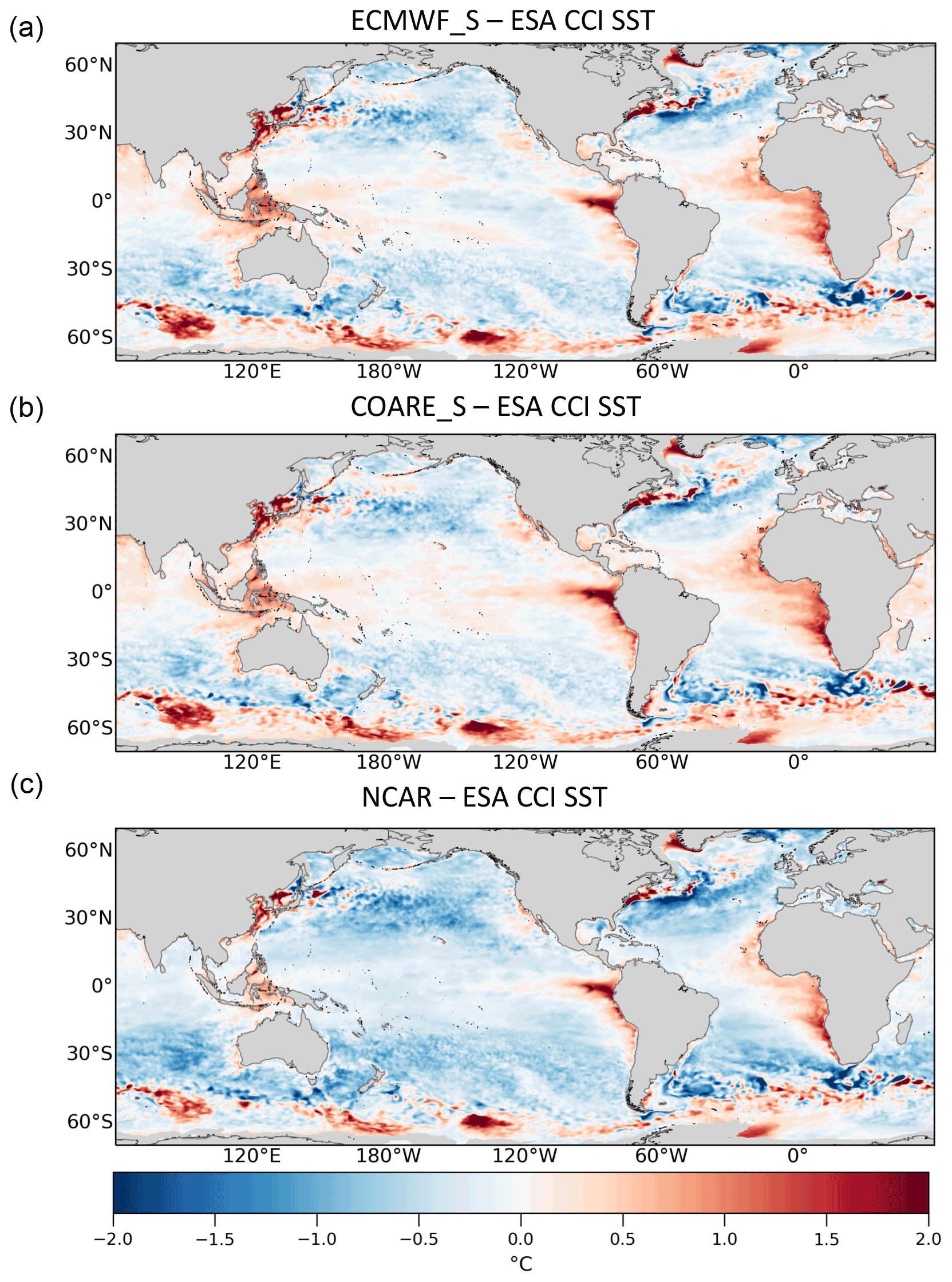
Figure 2Annual mean SST differences for (a) ECMWF_S, (b) COARE_S, and (c) NCAR versus the ESA CCI SST.
Figure 3Annual mean differences between ECMWF_S and NCAR experiments (left) and between COARE_S and NCAR experiments (right) in (a) wind stress (τ), (b) total turbulent heat flux (QT), and (c) wind stress curl (WSC). Hatching indicates significant values (95 % confidence level).
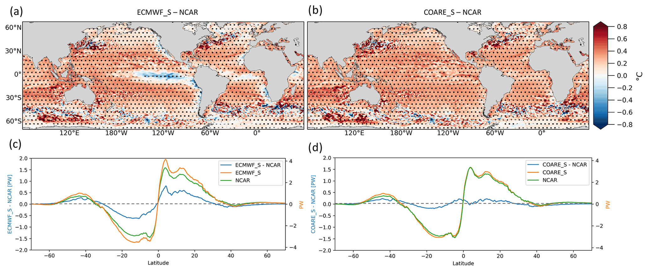
Figure 4Annual mean SST differences between (a) ECMWF_S − NCAR and (b) COARE_S − NCAR. Global meridional heat transport computed in the upper 100 m of the ocean for (c) ECMWF_S and NCAR and their differences; and for (d) COARE_S and NCAR and their differences. Right (left) y axes represent the MHT for single experiments (MHT difference). Hatching indicates significant values (95 % confidence level).
3.2 Skin temperature
The ECMWF and COARE parameterizations, in contrast to NCAR, expect SSTskin as the surface temperature input in order to estimate the near-surface atmospheric stability and to compute the THFs. The SSTskin is also used to estimate the upward long-wave flux, which is required by the CSWL scheme as a component of the NSHFs.
We now compare the results between ECMWF_S and ECMWF_NS to understand the impact of the CSWL implementation in causing the differences in the THFs and thus in the SSTs shown in Fig. 4 (see Table 1 for experimental details). We discuss the impact of the use of skin temperature on the ECMWF parameterization; however, similar results were found using COARE (not shown).
The ECMWF_S experiment uses the CSWL scheme, so Ts≡SSTskin is used to compute THFs, as opposed to ECMWF_NS, in which Ts≡SST.
Consideration of the CSWL effect yields an SST global mean warming of 0.2 ∘C (Fig. 5c), with a maximum of 0.3 ∘C over the western equatorial Pacific Ocean, in the Indo-Pacific Warm Pool.
In the tropical eastern and northern Pacific Ocean, and over the ACC, the differences are below 0.1 ∘C.
The global-mean SSTskin tends to be about 0.1 ∘C colder than the SST (Fig. 5a). On a global average basis, the cool skin process predominates over the warm layer effect. Specifically, evaporation occurs almost everywhere and most of the time, while the warm layer builds up only under sunny and low-wind conditions.
The colder Ts in ECMWF_S with respect to ECMWF_NS yields slightly weaker heat loss to the atmosphere due to the decreased NSHFs (mostly evaporation). In ECMWF_S, the weaker heat loss to the atmosphere implies a heat gain by the ocean (positive regions in Fig. 5b) of approximately 1 W m−2 on average globally compared to ECMWF_NS.
We can conclude that the negative SST discrepancies between parameterizations noted in Sect. 3.1 (Fig. 4a) are not explained by the use of the CSWL scheme in the ECMWF parameterization. Nevertheless, the CSWL scheme has a large impact on the positive SST difference between ECMWF_S and NCAR. The SST differences between ECMWF_NS and NCAR (Fig. 6a) with respect to the SST differences between ECMWF_S and NCAR (Fig. 4) present a reduction in the overall warm temperature differences.
τ and WSC differences are shown in Fig. S1 in the Supplement.
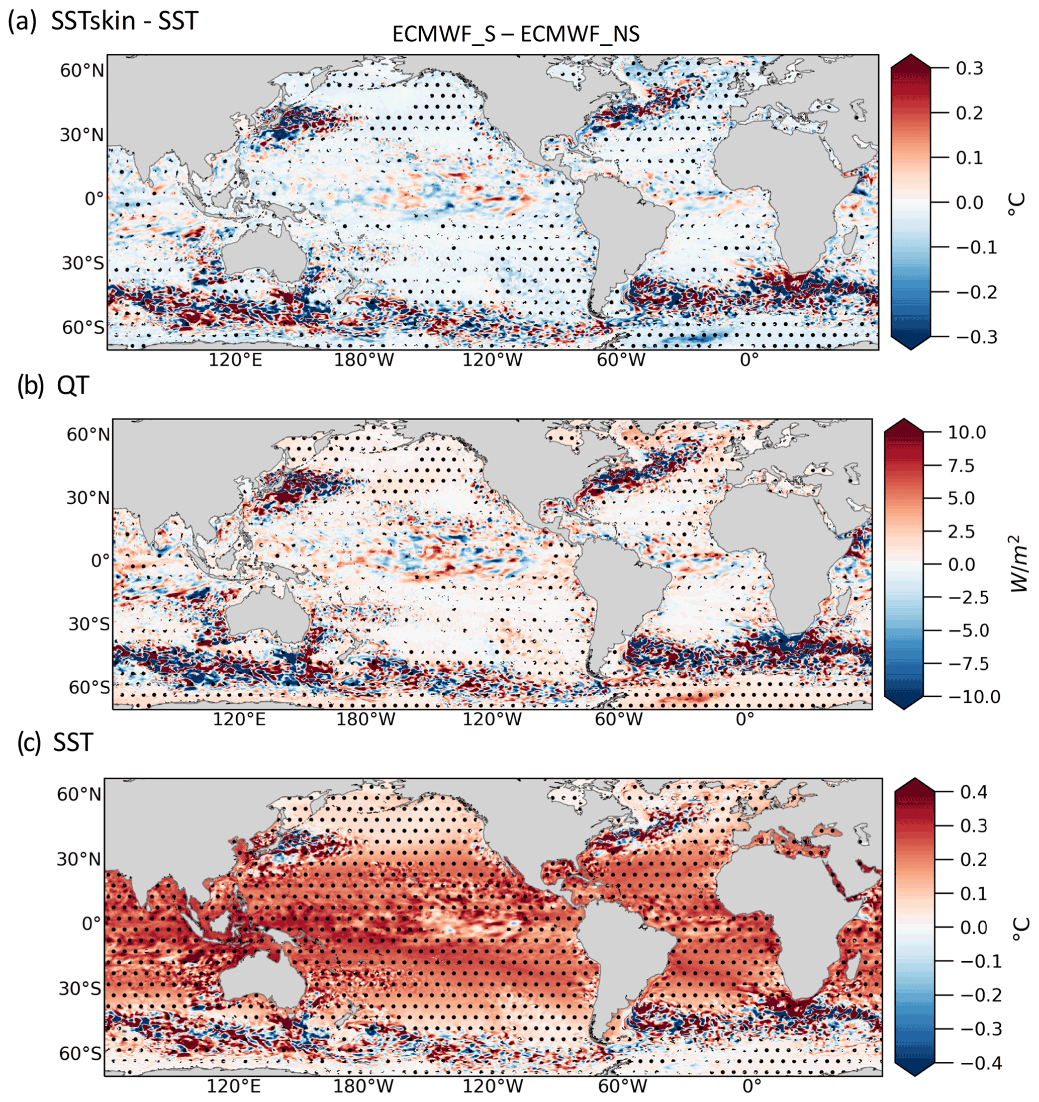
Figure 5Annual mean differences in (a) SSTskin (of ECMWF_S) − SST (of ECMWF_NS). Annual mean differences in (b) total turbulent heat flux (QT), and (c) SST between ECMWF_S and ECMWF_NS. Hatching indicates significant values (95 % confidence level).
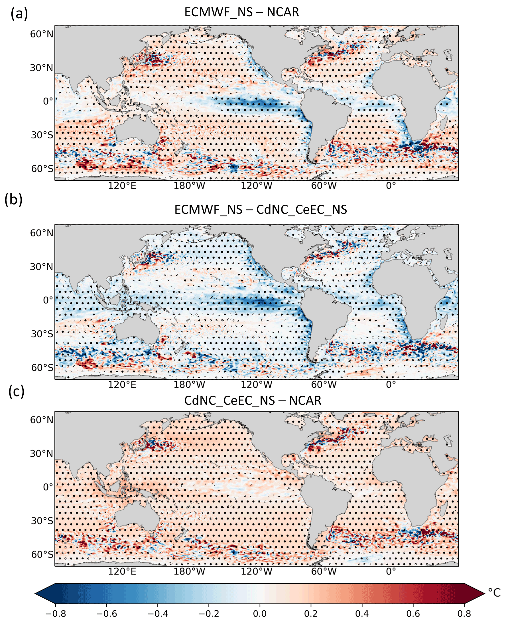
Figure 6Annual mean SST differences: (a) ECMWF_NS − NCAR, (b) ECMWF_NS − CdNC_CeEC_NS, and (c) CdNC_CeEC_NS − NCAR. Hatching indicates significant values (95 % confidence level).
3.3 Turbulent heat fluxes
In order to investigate the effect of the different computations of the THFs in ECMWF_S and NCAR in driving SST differences (Fig. 4a), we compared the results between CdNC_CeEC_NS and NCAR (see Table 1 for experimental details).
The SST difference between CdNC_CeEC_NS and NCAR does not show the cold bias over the EBUS and over the equatorial Atlantic and Pacific that we found between the experiments ECMWF_S and NCAR (compare Fig. 4a with Fig. 6c). Over those areas, the SST in CdNC_CeEC_NS is warmer than that in NCAR by about 0.3 ∘C on average.
As shown in Fig. 7a, CdNC_CeEC_NS receives an excess of QT of about 1 W m−2 on average with respect to NCAR.
The main contributor to this difference is the latent heat (Figs. 7a and 8b) resulting from the use of a different CE in the two experiments.
The CE of CdNC_CeEC_NS, which is smaller than the CE of NCAR (Fig. 8a), induces weak evaporation. The resulting weaker heat loss to the atmosphere in CdNC_CeEC_NS with respect to NCAR implies a gain of heat by the ocean (positive regions in Fig. 7a) of about 2 W m−2 over low latitudes and up to 6 W m−2 over mid-latitudes (Fig. 7b).
A similar process also occurs in areas where the annual mean pattern of QT is patchy due to mesoscale activities in both summer and winter (e.g., in the Western Boundary Currents, Fig. S2). In CdNC_CeEC_NS, the negative virtual temperature differences at the air–sea interface are smaller than in NCAR, inducing weaker heat losses from the ocean to the atmosphere.
It is worth mentioning that the 1 year simulation might not be adequate to properly represent the mean state in WBC regions due to the chaotic dynamics of these regions – this may explain some of the noise in the difference maps. However, this does not affect the robustness of the results.
The differences in QT and SST have the same sign, which suggests that QT drives the SST differences. As is clearly shown by the annual zonally averaged differences (Fig. 7b), the weaker the heat loss from the ocean in CdNC_CeEC_NS along a latitude, the warmer the ocean modeled by the CdNC_CeEC_NS experiment with respect to NCAR.
τ and WSC differences are shown in Fig. S3.
In summary, weak evaporation and thus weaker heat loss in CdNC_CeEC_NS generates an ocean surface temperature that is warmer than in NCAR.
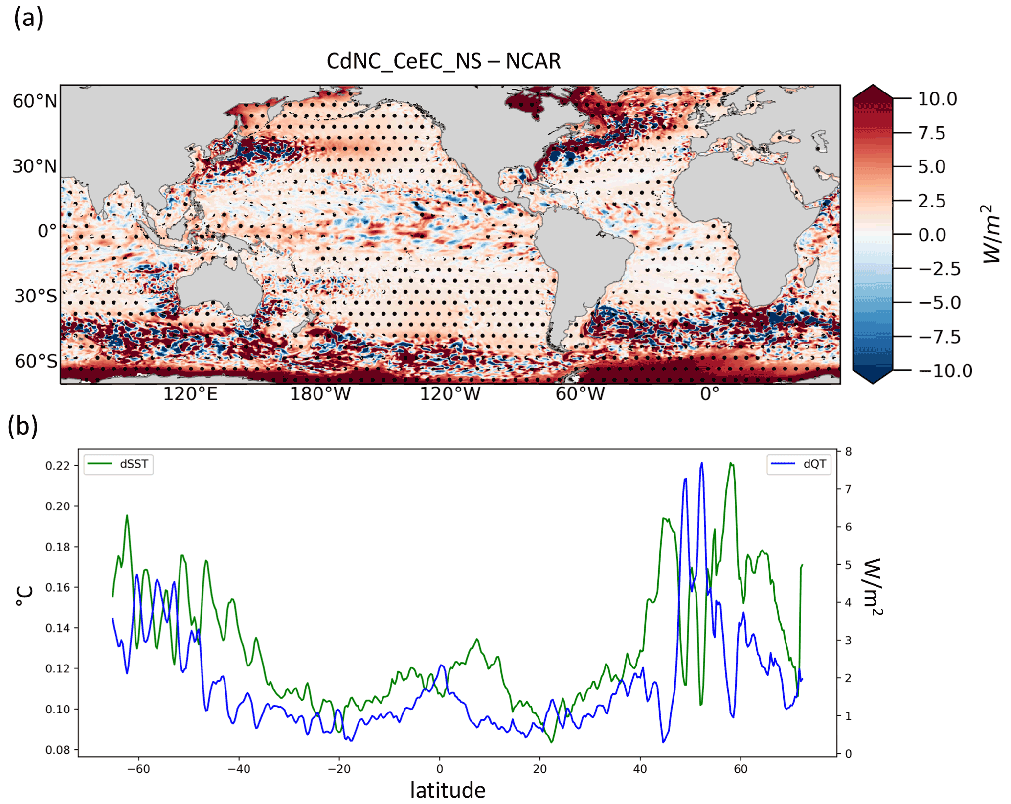
Figure 7(a) Annual mean differences in total turbulent heat fluxes QT between the CdNC_CeEC_NS and NCAR experiments. (b) Zonally averaged differences in SST (green) and QT (blue) annual means between the same experiments. Hatching indicates significant values (95 % confidence level).
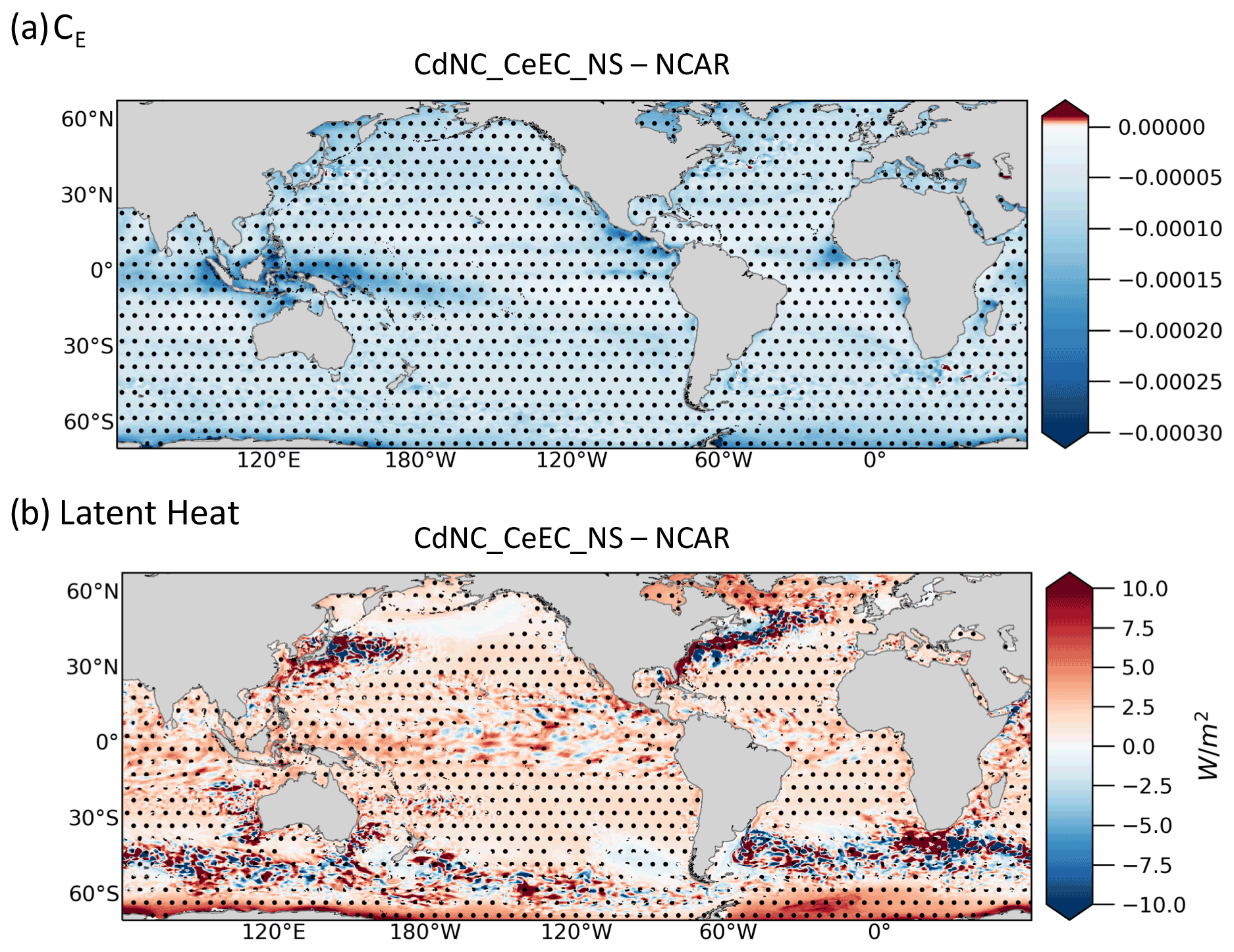
Figure 8Annual mean differences in (a) specific humidity transfer coefficient (CE) and (b) latent heat between CdNC_CeEC_NS and NCAR.
3.4 Drag coefficient and wind stress
We investigated the impact of the wind stress in driving the SST differences between the ECMWF_S and NCAR bulk parameterizations by comparing results from ECMWF_NS and CdNC_CeEC_NS simulations (see Table 1 for experimental details). CdNC_CeEC_NS differs from ECMWF_NS in its use of a different algorithm to compute CD and the inclusion of gustiness in the stress computation.
The SST simulated by ECMWF_NS is colder than that simulated by CdNC_CeEC_NS over the EBUS and the tropical Pacific and Atlantic oceans (Fig. 6b), which are characterized by wind-driven upwelling. This suggests that wind stress is a major driver of the SST differences (Fig. 4a).
Referring to Eq. (1a), the wind stress is proportional to the wind speed vector at height z (uz), the bulk scalar wind speed U (with the potential inclusion of a gustiness contribution), and the drag coefficient (CD).
Since U does not depend on the SST or on CD, including gustiness in the ECMWF calculation produces the scalar wind speed differences shown in Fig. 9a.
As expected, the differences caused by the gustiness correction, which do not exceed 0.3 m s−1, emerge in regions with calm and unstable conditions. These areas are in fact located in the 5–10∘ N latitude band, in the eastern Pacific and Atlantic oceans, in the tropical western Pacific including the South China Sea, and the tropical Indian Ocean. Differences in the CD and fields between experiments show similar patterns (Fig. 9b–c), suggesting that the differences in CD between parameterizations are related to the neutral coefficient () calculation rather than to its stability correction (the term to add to to obtain CD coefficients). In fact, as discussed in Sect. 2.2 for , the ECMWF CD is larger than that of NCAR for wind speeds above 5 m s−1, and smaller than that of NCAR for conditions ranging from calm to a light breeze (U<5 m s−1). In the areas where U is approximately 4–5 m s−1, such as in the northwest Pacific and the Atlantic oceans (between 20 and 30∘ N) and in the southeast Pacific and the Atlantic oceans (between 20 and 30∘ S), the ECMWF CD is similar to or slightly smaller than that of NCAR.
Since the wind stress is not affected by the type of first-order feedback at play for the NSHFs (SST–QT negative feedback, see Sect. 2.2), differences in U and CD between experiments are reflected in the resulting different fields after bulk calculation (i.e., τ and WSC, Fig. 10).
Over the ACC, the northern and southern mid-latitudes (e.g., the EBUS), and the Atlantic storm track (i.e., regions characterized by wind speeds above 5 m s−1 and with ECMWF_NS CD larger than CdNC_CeEC_NS CD, see Fig. 10), the ECMWF_NS wind stress is stronger with respect to NCAR by an average of 0.035 N m−2 (about 20 % of the absolute value in NCAR).
In the 5–10∘ N region, which is a latitudinal band characterized by mean winds below 5 m s−1 and larger CD values in CdNC_CeEC_NS than in ECMWF_NS (Fig. 10), ECMWF_NS shows a wind stress reduction of −0.003 N m−2 (about 3 % of NCAR absolute value) with respect to NCAR.
In regions where the differences in CD and wind stress are opposite (e.g., the northwest and southwest Pacific and Atlantic oceans, the Indian Ocean, Baja California, the Equatorial Warm Pool), the inclusion of convective gustiness in the U calculation may play a role in strengthening the wind stress in ECMWF_NS (Fig. 9a). In addition, the high time variability of the CD differences (not shown) could hide the relation between CD and τ.
Both hypotheses are verified: the ECMWF_NS experiment presents a stronger wind stress almost everywhere over the global ocean compared to a twin experiment (i.e., ECMWF_NS_NG) where the convective gustiness is not used in the computation (Fig. S4), and the correlation between CD differences and wind stress differences is always significant and positive (not shown). The higher the difference in CD, the stronger the difference in wind stress.
The SST differences between ECMWF_NS and CdNC_CeEC_NS over the tropical Pacific and Atlantic oceans (Fig. 6b) are probably related to Ekman suction, which is driven by the positive (negative) wind stress curl in the Northern (Southern) Hemisphere.
Substantial differences were found in ECMWF_NS compared to CdNC_CeEC_NS, characterized by greater mean wind stress both north and south of the tropical band and weaker wind stress along the Equator (Fig. 10a).
These latitudinal differences in wind stress between experiments are reflected in the differences in the wind stress curl patterns (Fig. 10b). Indeed, a stronger acceleration (deceleration) of southeast trades north (south) of the Equator in ECMWF_NS may lead to a stronger positive (negative) curl north (south) of the Equator.
This relation was found to be significant north of the Equator: the stronger positive wind stress curl in ECMWF_NS than in CdNC_CeEC_NS resulted in a colder SST in ECMWF_NS compared to CdNC_CeEC_NS (see the correlation map in Fig. S5).
The stronger wind stress along the EBUS in ECMWF_NS compared to CdNC_CeEC_NS instead probably enhances coastal upwelling, explaining most of the SST differences over these regions. Part of the SST difference could also be related to Ekman suction. ECMWF_NS shows a stronger positive (negative) wind stress curl in the Northern (Southern) Hemisphere EBUS compared to CdNC_CeEC_NS (Fig. 10b). The vertical velocity and, in turn, the coastal SST along the EBUS are, indeed, extremely sensitive to wind forcing changes (Bonino et al., 2019; Small et al., 2015; Capet et al., 2004; Desbiolles et al., 2014).
These relations were confirmed to be present along the coast of the Benguela Upwelling System (Figs. S6 and S6). During the Benguela upwelling season (ONDJ = October-November-December-January), the enhanced wind stress and negative wind stress curl in ECMWF_NS reinforce the vertical velocity with respect to CdNC_CeEC_NS (Fig. S6), resulting in a colder surface temperature (see the correlation maps in Fig. S7).
The differences in wind stress are also responsible for the changes in meridional heat transport. MHT differences between ECMWF_NS and CdNC_CeEC_NS resemble the differences between ECMWF_S and NCAR (compare Figs. 4c and 11c), with higher transport in ECMWF_NS at all latitudes. The largest differences are located in the tropical region (up to 0.6 PW, about 18 % of the mean value in NCAR), where the differences in meridional transport (linked to the equatorial upwelling) between the two experiments are likely maxima.

Figure 9Annual mean differences in (a) wind speed (U), (b) neutral wind stress transfer coefficient (CDN), and (c) wind stress transfer coefficient (CD) between ECMWF_NS and CdNC_CeEC_NS. Hatching indicates significant values (95 % confidence level).
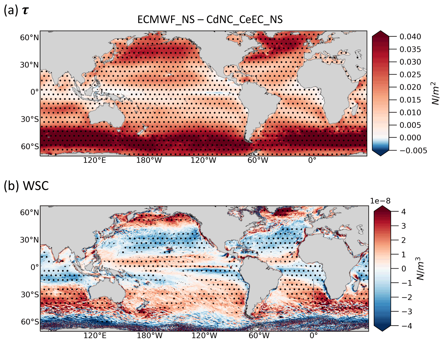
Figure 10Annual mean differences in (a) wind stress (τ) and (b) wind stress curl (WSC) between ECMWF_NS and CdNC_CeEC_NS.
Although the two experiments use the same CE and CH, the dependence of QL and QH on the prognostic SST at each time step generates differences in QT (Fig. 11a).
The ocean gains heat in ECMWF_NS compared to CdNC_CeEC_NS (i.e., positive QT differences) over the EBUS and the equatorial region.
In contrast to the previous finding, the differences in QT and SST have opposite signs, indicating that SST differences drive the QT differences: the colder the temperature produced by ECMWF_NS wind stress with respect to CdNC_CeEC_NS, the higher the heat gained by ECMWF_NS along the latitudes (Fig. 11b).
In summary, ECMWF_NS reproduces stronger wind stress and wind stress curl along the EBUS and stronger cyclonic wind stress curl along the Equator, which generate colder SSTs with respect to CdNC_CeEC_NS through enhanced upwelling processes.
Given the importance of wind stress in driving the SST differences between the ECMWF and NCAR parameterizations, we now examine why COARE_S does not show the cold SST differences in comparison to NCAR over the EBUS and the equatorial Pacific (Fig. 4b). With wind speeds ranging from 7 to 9 m s−1 (e.g., over the EBUS), the CD in the COARE_S parameterization is smaller than that of the ECMWF parameterization but slightly higher than or almost identical to (around 7 m s−1) the CD of NCAR (refer to Fig. 1c). Moreover, over the northern equatorial band, the CD of COARE_S is smaller than that of ECMWF_S and NCAR. As a consequence, the COARE_S differences in wind stress (Fig. 3a) in comparison with NCAR are characterized by a strong decrease – roughly 10 % – over the northern equatorial band, and a slight increase in the wind stress – roughly 2 % – over the EBUS. The increase in wind stress over the EBUS in COARE_S (2 % in comparison to the increase of 25 % that occurs over the EBUS in ECMWF_S) is insufficient to promote stronger coastal upwelling in the annual mean and, in turn, a colder SST with respect to NCAR.
As regards the equatorial upwelling, the weak increase in the wind stress in the northern equatorial region (e.g., the northern equatorial cold front) compared to the NCAR wind stress (Fig. 3a) prevents the enhancement of the positive wind stress curl in COARE_S (Fig. 3c). However, to properly identify the drivers of the pattern of SST differences between COARE_S and NCAR, further numerical experiments need to be performed.
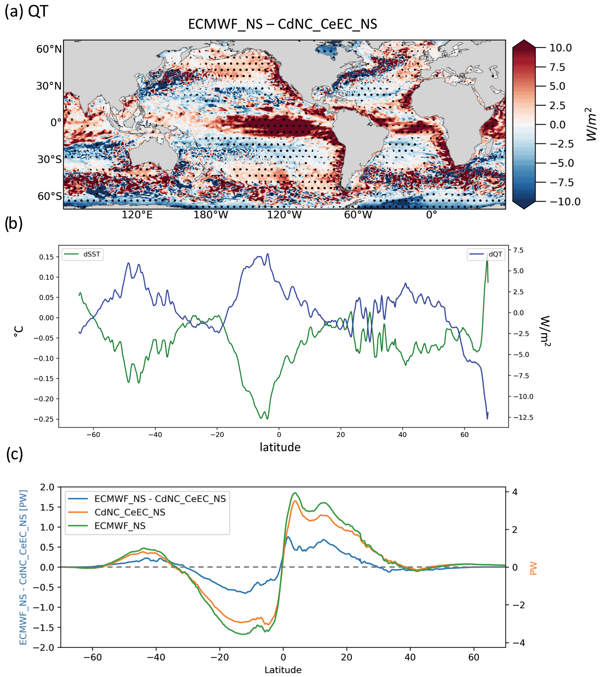
Figure 11(a) Annual mean differences in turbulent heat fluxes (QT) between ECMWF_NS and CdNC_CeEC_NS. (b) Time series of annual zonal-mean differences in SST (green) and QT (blue) between ECMWF_NS and CdNC_CeEC_NS. (c) Global meridional heat transport in the upper 100 m of the ocean (values on the right y axis) for ECMWF_NS and CdNC_CeEC_NS and differences (values on the left y axis) between them. Hatching indicates significant values (95 % confidence level).
3.5 Online prognostic SST approach vs. offline prescribed SST approach
In order to explore the role of the SST–QT negative feedback at play in the online prognostic SST approach, we compared our results with those of Brodeau et al. (2017), who compared the different bulk parameterizations using the offline prescribed SST approach (i.e., TASFs are computed by means of bulk formulas using prescribed surface atmospheric variables and the prescribed SST).
There are a few differences in bulk implementation between this study and Brodeau et al. (2017). The latter authors used the COARE3.0 parameterization instead of COARE3.6, and their simulations, which were performed for a longer (1982–2014) period, were forced by the ERA-Interim reanalysis instead of ERA5. Our aim in this comparison is therefore only to qualitatively understand the negative feedback between the SST and the QT at play in our experiments.
Brodeau et al. (2017) report a mean global increase in the wind stress of 20 mN m−2 using ECMWF parameterization instead of NCAR parameterization. The computation of the wind stress is not affected by the SST–QT negative feedback (see Eq. 1a). This means that our result – the 20 mN m−2 global mean increase in wind stress – is completely in line with the prescribed SST comparison by Brodeau et al. (2017).
Our findings do not follow Brodeau et al. (2017) in terms of the QT differences between the ECMWF_S and NCAR parameterizations. The latter authors found a global mean increase in QT of 13 W m−2 for ECMWF_S, while in our experiments, ECMWF_S showed a mean global increase of 5 W m−2 with respect to NCAR. Moreover, they report an increase of 7 W m−2 by considering the SSTskin rather than the SST in the COARE parameterization, while in our experiments, ECMWF_S showed a mean global increase of 1 W m−2 with respect to ECMWF_NS.
The negative feedback between the SST and the QT which is active in our experiments reduced the differences in the total turbulent flux across parameterizations compared to the prescribed SST comparison.
In this work, we have investigated how the implementation of different bulk parameterizations in the NEMOv4 ocean general circulation model drives substantial changes in prognostic sea surface temperature. Specifically, we studied the contributions of different aspects and assumptions of the bulk parameterizations in driving the SST differences across numerical experiments performed using the NEMO global model configuration with ∘ of horizontal resolution. We analyzed and quantified the role of the inclusion of the skin temperature in the computation of the turbulent heat flux components, and we also studied the roles of the turbulent heat flux components and the wind stress in driving the SST changes between parameterizations. We analyzed annual mean TASF differences between “control experiments”, short-term numerical experiments which used the bulk parameterizations implemented in NEMOv4, and “mixed experiments”, short-term sensitivity experiments where bulk assumptions were excluded (e.g., skin temperature) or bulk transfer coefficients were computed by mixing the bulk parameterizations (e.g., CD from NCAR parameterization and CE and CH from ECMWF parameterization). In addition to highlighting the sensitivity of the sea surface temperature to the bulk parameterizations, we believe that the importance of this work is also the examination of the role of the SST–QT negative feedback in the simulations. We compared the modeled turbulent air–sea fluxes with the estimations by Brodeau et al. (2017), who analyzed the same bulk parameterizations but used the offline prescribed SST approach. Our findings can be summarized as follows:
-
The implementation of skin temperature in the bulk parameterizations reduces evaporation and decreases the turbulent heat flux to the atmosphere, thus promoting ocean warming. The skin temperature is usually colder than the sea surface temperature. The skin temperature contribution in terms of turbulent heat flux is weaker than the estimations from Brodeau et al. (2017) due to the negative feedback between the SST and the QT. In our experiments, SST was free to evolve and fed back negatively with respect to QT.
-
The turbulent heat flux differences between experiments are dominated by the latent heat flux, which arises from CE differences between bulk parameterizations. A less evaporative ocean gains heat, which tends to promote ocean warming. The turbulent heat flux differences are weaker than the estimations of Brodeau et al. (2017) and can be attributed to the SST–QT negative feedback.
-
The wind stress differences between bulk parameterizations are attributable to the CD differences, especially in wind-driven dominantly ocean regions. Experiments with enhanced wind stress or wind stress curl over the EBUS and over the equatorial Pacific promote upwelling processes and consequent cooling of the sea surface temperature. Stronger wind stress causes an increase in the poleward heat transport in the upper ocean, which leads to a more pronounced increase in the ±20∘ N latitude band. The wind stress differences among the bulk parameterizations implemented in NEMOv4 are of the same magnitude as the wind stress differences calculated by Brodeau et al. (2017). This is due to the fact that, at first order, the wind stress computation is not affected by the SST.
We used forced ocean experiments in which the atmospheric fields (e.g., wind, air temperature, air humidity) in the ocean model and seen in the online prognostic SST approach come from an atmospheric reanalysis and do not feed back to the ocean variability. Introducing the air–sea feedback into the system might substantially impact on the turbulent fluxes and modify our findings in terms of comparing the SST response among the bulk parameterizations. In order to improve the representation of the air–sea interaction in the NEMO framework, an atmospheric boundary layer (ABL) was integrated into the new NEMO release 4.2 (Lemarié et al., 2021). However, this ABL implementation is at a preliminary stage, and the current online prognostic SST approach is still the most commonly used. Although the new release of NEMO, v4.2, includes some modifications to the bulk formula version used in this study, these changes do not affect the results presented in this paper.
| Acronym | Expansion |
| TASFs | Turbulent air–sea flux components |
| THFs | Turbulent heat flux components |
| NSHFs | Non-solar heat flux components |
| QT | Total turbulent heat flux |
| BTC | Bulk transfer coefficient |
| SSTskin | Sea surface skin temperature |
| CSWL | Cool skin and (diurnal) warm layer |
| EBUS | Eastern Boundary Upwelling Systems |
| MHT | Meridional heat transport |
| WSC | Wind stress curl |
The NEMO code and the namelists used to run each experiment are available in the Zenodo archive (https://doi.org/10.5281/zenodo.6258085, Bonino, 2022). This version of the NEMO code is based on release 4.0 (Madec and the NEMO System Team, 2019), revision number 12957 (https://forge.ipsl.jussieu.fr/nemo/browser/NEMO/trunk?rev=12957, last access: 24 February 2022). The original code was modified in the computations of the bulk transfer coefficients applied to perform the experiments.
The model outputs used to produce the figures are available in the Zenodo archive (https://doi.org/10.5281/zenodo.6258085, Bonino, 2022).
The supplement related to this article is available online at: https://doi.org/10.5194/gmd-15-6873-2022-supplement.
GB modified the numerical code, set up the experiment and wrote the manuscript. DI conceived and designed this study. GB, DI, LB and SM contributed to the interpretation of results and editing.
The contact author has declared that none of the authors has any competing interests.
Publisher’s note: Copernicus Publications remains neutral with regard to jurisdictional claims in published maps and institutional affiliations.
We acknowledge the CMCC Foundation for providing computational resources.
This research has been supported by the EU project IMMERSE (H2020 grant agreement no. 821926).
This paper was edited by Riccardo Farneti and reviewed by Justin Small and two anonymous referees.
Amante, C. and Eakins, B. W.: ETOPO1 1 Arc-Minute Global Relief Model: Procedures, Data Sources and Analysis, NOAA Technical Memorandum NESDIS NGDC-24, National Geophysical Data Center, NOAA [data set], https://doi.org/10.7289/V5C8276M, 2009. a
Barnier, B.: Forcing the Ocean, in: Ocean Modeling and Parameterization, edited by: Chassignet, E. P. and Verron, J., NATO Science Series, vol 516, Springer, 45–80, https://doi.org/10.1007/978-94-011-5096-5_2, 1998. a
Barnier, B., Madec, G., Penduff, T., Molines, J. M., Treguier, A. M., Le Sommer, J., Beckmann, A., Biastoch, A., Böning, C., Dengg, J., Derval, C., Durand, E., Gulev, S., Remy, E., Talandier, C., Theetten, S., Maltrud, M., McClean, J., and De Cuevas, B.: Impact of partial steps and momentum advection schemes in a global ocean circulation model at eddy-permitting resolution, Ocean Dynam., 56, 543–567, https://doi.org/10.1007/s10236-006-0082-1, 2006. a
Blanke, B. and Delecluse, P.: Variability of the tropical Atlantic Ocean simulated by a general circulation model with two different mixed-layer physics, J. Phys. Oceanogr., 23, 1363–1388, 1993. a
Bonino, G.: The bulk parameterizations of turbulent air-sea fluxes in NEMO4: the origin of Sea Surface Temperature differences in a global model study, Zenodo [code and data set], https://doi.org/10.5281/zenodo.6258085, 2022. a, b
Bonino, G., Masina, S., Iovino, D., Storto, A., and Tsujino, H.: Eastern Boundary Upwelling Systems response to different atmospheric forcing in a global eddy-permitting ocean model, J. Marine Syst., 197, 103178, https://doi.org/10.1016/j.jmarsys.2019.05.004, 2019. a
Bonino, G., Iovino, D., and Masina, S.: Bulk Formulations in NEMOv.4:algorithms review and sea surface temperature response in ORCA025case study, Technical Notes No. 289, https://doi.org/10.25424/cmcc/bulk_formulas_nemo_report, 2020. a
Bradley, E. and Fairall C.: A Guide to Making Climate Quality Meteorological and Flux Measurements at Sea, NOAA Technical Memorandum OAR PSD-311, NOAA/ESRL/PSD, Boulder, CO, 108, 2007. a
Brodeau, L., Barnier, B., Gulev, S. K., and Woods, C.: Climatologically significant effects of some approximations in the bulk parameterizations of turbulent air–sea fluxes, J. Phys. Oceanogr., 47, 5–28, 2017. a, b, c, d, e, f, g, h, i, j, k, l, m, n, o
Capet, X., Marchesiello, P., and McWilliams, J: Upwelling response to coastal wind profiles, Geophys. Res. Lett., 31, L13311, https://doi.org/10.1029/2004GL020123, 2004. a
Chen, D., Busalacchi, A. J., and Rothstein, L. M.: The roles of vertical mixing, solar radiation, and wind stress in a model simulation of the sea surface temperature seasonal cycle in the tropical Pacific Ocean, J. Geophys. Res.-Oceans, 99, 20345–20359, 1994. a
Dai, A. and Trenberth, K. E.: Estimates of freshwater discharge from continents: Latitudinal and seasonal variations, J. Hydrometeorol., 3, 660–687, 2002. a
Dai, A., Qian, T., Trenberth, K. E., and Milliman, J. D.: Changes in continental freshwater discharge from 1948 to 2004, J. Climate, 22, 2773–2792, 2009. a
Desbiolles, F., Blanke, B., Bentamy, A., and Grima, N.: Origin of fine-scale wind stress curl structures in the Benguela and Canary upwelling systems, J. Geophys. Res.-Oceans, 119, 7931–7948, https://doi.org/10.1002/2014JC010015, 2014. a
Desbiolles, F., Alberti, M., Hamouda, M. E., Meroni, A. N., and Pasquero, C.: Links between sea surface temperature structures, clouds and rainfall: Study case of the Mediterranean Sea, Geophys. Res. Lett., 48, e2020GL091839, https://doi.org/10.1029/2020GL091839, 2021. a
de Szoeke, S. P., Marke, T., and Brewer, W. A.: Diurnal ocean surface warming drives convective turbulence and clouds in the atmosphere, Geophys. Res. Lett., 48, e2020GL091299, https://doi.org/10.1029/2020GL091299, 2021. a
Edson, J. B., Jampana, V., Weller, R. A., Bigorre, S. P., Plueddemann, A. J., Fairall, C. W., Miller, S. D., Mahrt, L., Vickers, D., and Hersbach, H.: On the exchange of momentum over the open ocean, J. Phys. Oceanogr., 43, 1589–1610, 2013. a, b
Fairall, C. W., Bradley, E. F., Rogers, D. P., Edson, J. B., and Young, G. S.: Bulk parameterization of air-sea fluxes for tropical ocean-global atmosphere coupled-ocean atmosphere response experiment, J. Geophys. Res.-Oceans, 101, 3747–3764, 1996. a
Fairall, C. W., Bradley, E. F., Hare, J., Grachev, A. A., and Edson, J. B.: Bulk parameterization of air–sea fluxes: Updates and verification for the COARE algorithm, J. Climate, 16, 571–591, 2003. a
Gaube, P., Chickadel, C., Branch, R., and Jessup, A.: Satellite observations of SST-induced wind speed perturbation at the oceanic submesoscale, Geophys. Res. Lett., 46, 2690–2695, 2019. a
Gill, A. E.: Atmosphere-ocean dynamics, Int. Geophys. Ser., 30, 662, https://books.google.de/books?hl=en&lr=&id=1WLNX_lfRp8C&oi=fnd&pg=PR11&ots=Tr4Y05QSgT&sig=WvPiasaS4Rgcdu7L97z2uH1wrEs&redir_esc=y#v=onepage&q&f=false (last access: 1 September 2022), 1982. a
Hersbach, H., Bell, B., Berrisford, P., Hirahara, S., Horányi, A., Muñoz-Sabater, J., Nicolas, J., Peubey, C., Radu, R., Schepers, D., et al.: The ERA5 global reanalysis, Q. J. Roy. Meteor. Soc., 146, 1999–2049, 2020. a, b
IOC and IHO: BODC. Centenary Edition of the GEBCO Digital Atlas, published on CD-ROM on behalf of the Intergovernmental Oceanographic Commission (IOC) and the International Hydrographic Organization (IHO) as part of the General Bathymetric Chart of the Oceans, British Oceanographic Data Centre, Liverpool, 2003. a
Jacobs, S. S., Hellmer, H. H., and Jenkins, A.: Antarctic ice sheet melting in the Southeast Pacific, Geophys. Res. Lett., 23, 957–960, 1996. a
Kara, A. B., Rochford, P. A., and Hurlburt, H. E.: Efficient and accurate bulk parameterizations of air–sea fluxes for use in general circulation models, J. Atmos. Ocean. Tech., 17, 1421–1438, 2000. a, b
Large, W. and Pond, S.: Open ocean momentum flux measurements in moderate to strong winds, J. Phys. Oceanogr., 11, 324–336, 1981. a
Large, W. and Pond, S.: Sensible and latent heat flux measurements over the ocean, J. Phys. Oceanogr., 12, 464–482, 1982. a
Large, W. and Yeager, S.: The global climatology of an interannually varying air–sea flux data set, Clim. Dynam., 33, 341–364, 2009. a
Lemarié, F., Samson, G., Redelsperger, J.-L., Giordani, H., Brivoal, T., and Madec, G.: A simplified atmospheric boundary layer model for an improved representation of air–sea interactions in eddying oceanic models: implementation and first evaluation in NEMO (4.0), Geosci. Model Dev., 14, 543–572, https://doi.org/10.5194/gmd-14-543-2021, 2021. a, b, c
Levitus, S., Antonov, J., Baranova, O., Boyer, T., Coleman, C., Garcia, H., Grodsky, A., Locarnini, R., Mishonov, A., Reagan, J., Sazama, C. L., Seidov, D., Smolyar, I., Yarosh, E. S., and Zweng, M. M.: The world ocean database, Data Science Journal, 12, WDS229–WDS234, 2013. a
Li, Y. and Carbone, R.: Excitation of rainfall over the tropical western Pacific, J. Atmos. Sci., 69, 2983–2994, 2012. a
Madec, G. and Imbard, M.: A global ocean mesh to overcome the North Pole singularity, Clim. Dynam., 12, 381–388, 1996. a
Madec, G. and NEMO System Team: Nemo ocean engine – version 4.0.1, Scientific Notes of Climate Modelling Center (27) – ISSN 1288-1619, Institut Pierre-Simon Laplace (IPSL), https://doi.org/10.5281/zenodo.3878122, 2019 (code of revision 12957 available at: (https://forge.ipsl.jussieu.fr/nemo/browser/NEMO/trunk?rev=12957, last access: 24 February 2022). a, b
Merchant, C. J., Embury, O., Bulgin, C. E., Block, T., Corlett, G. K., Fiedler, E., Good, S. A., Mittaz, J., Rayner, N. A., Berry, D., Eastwood, S., Taylor, M., Tsushima, Y., Waterfall, A., Wilson, R., and Donlon, C.: Satellite-based time-series of sea-surface temperature since 1981 for climate applications, Scientific Data, 6, 223, https://doi.org/10.1038/s41597-019-0236-x, 2019. a
Monin, A. S. and Obukhov, A. M.: Basic laws of turbulent mixing in the surface layer of the atmosphere, Contrib. Geophys. Inst. Acad. Sci. USSR, 151, e187, https://moodle2.units.it/pluginfile.php/267453/mod_resource/content/1/ABL_lecture_13.pdf (last access: 1 September 2022), 1954. a
NEMO Sea Ice Working Group: Sea Ice modelling Integrated Initiative (SI3) – The NEMO sea ice engine, Scientific Notes of Climate Modelling Center (31) – ISSN 1288-1619, Institut Pierre-Simon Laplace (IPSL), Zenodo, https://doi.org/10.5281/zenodo.3878122, 2019. a
Renault, L., Lemarié, F., and Arsouze, T.: On the implementation and consequences of the oceanic currents feedback in ocean–atmosphere coupled models, Ocean Model., 141, 101423, https://doi.org/10.1016/j.ocemod.2019.101423, 2019a. a
Renault, L., Masson, S., Oerder, V., Jullien, S., and Colas, F.: Disentangling the mesoscale ocean-atmosphere interactions, J. Geophys. Res.-Oceans, 124, 2164–2178, 2019b. a
Renault, L., Masson, S., Arsouze, T., Madec, G., and Mcwilliams, J. C.: Recipes for how to force oceanic model dynamics, J. Adv. Model. Earth Sy., 12, e2019MS001715, https://doi.org/10.1029/2019MS001715, 2020. a
Seager, R., Blumenthal, M. B., and Kushnir, Y.: An advective atmospheric mixed layer model for ocean modeling purposes: Global simulation of surface heat fluxes, J. Climate, 8, 1951–1964, 1995. a
Shriver, J. F. and Hurlburt, H. E.: The contribution of the global thermohaline circulation to the Pacific to Indian Ocean throughflow via Indonesia, J. Geophys. Res.-Oceans, 102, 5491–5511, 1997. a
Siedler, G., Griffies, S. M., Gould, J., and Church, J. A.: Ocean circulation and climate: a 21st century perspective, Academic Press, eBook ISBN 9780123918536, Hardcover ISBN 9780123918512, 2013. a
Small, R. D., deSzoeke, S. P., Xie, S., O’Neill, L., Seo, H., Song, Q., Cornillon, P., Spall, M., and Minobe, S.: Air–sea interaction over ocean fronts and eddies, Dynam. Atmos. Oceans, 45, 274–319, 2008. a, b
Small, R. J., Curchitser, E., Hedstrom, K., Kauffman, B., and Large, W. G.: The Benguela upwelling system: Quantifying the sensitivity to resolution and coastal wind representation in a global climate model, J. Climate, 28, 9409–9432, 2015. a
Smith, S. D.: Coefficients for sea surface wind stress, heat flux, and wind profiles as a function of wind speed and temperature, J. Geophys. Res.-Oceans, 93, 15467–15472, 1988. a
Sun, Z., Liu, H., Lin, P., Tseng, Y.-H., Small, J., and Bryan, F.: The modeling of the North Equatorial Countercurrent in the Community Earth System Model and its oceanic component, J. Adv. Model. Earth Sy., 11, 531–544, 2019. a
Swenson, M. S. and Hansen, D. V.: Tropical Pacific Ocean mixed layer heat budget: The Pacific cold tongue, J. Phys. Oceanogr., 29, 69–81, 1999. a
Torres, O., Braconnot, P., Marti, O., and Gential, L.: Impact of air-sea drag coefficient for latent heat flux on large scale climate in coupled and atmosphere stand-alone simulations, Clim. Dynam., 52, 2125–2144, 2019. a
Yuen, C., Cherniawsky, J., Lin, C., and Mysak, L.: An upper ocean general circulation model for climate studies: Global simulation with seasonal cycle, Clim. Dynam., 7, 1–18, https://doi.org/10.1007/BF00204817, 1992. a
Zalesak, S. T.: Fully multidimensional flux-corrected transport algorithms for fluids, J. Comput. Phys., 31, 335–362, 1979. a
- Abstract
- Introduction
- Model configuration, bulk forcing, and experimental setup
- Results
- Summary and conclusions
- Appendix A: List of acronyms and symbols
- Code availability
- Data availability
- Author contributions
- Competing interests
- Disclaimer
- Acknowledgements
- Financial support
- Review statement
- References
- Supplement