the Creative Commons Attribution 4.0 License.
the Creative Commons Attribution 4.0 License.
 | 06 Sep 2022
Intercomparison of four algorithms for detecting tropical cyclones using ERA5
Stella Bourdin
Sébastien Fromang
William Dulac
Julien Cattiaux
Fabrice Chauvin
The assessment of tropical cyclone (TC) statistics requires the direct, objective, and automatic detection and tracking of TCs in reanalyses and model simulations. Research groups have independently developed numerous algorithms during recent decades in order to answer that need. Today, there is a large number of trackers that aim to detect the positions of TCs in gridded datasets. The questions we ask here are the following: does the choice of tracker impact the climatology obtained? And, if it does, how should we deal with this issue?
This paper compares four trackers with very different formulations in detail. We assess their performances by tracking TCs in the ERA5 reanalysis and by comparing the outcome to the IBTrACS observations database.
We find typical detection rates of the trackers around 80 %. At the same time, false alarm rates (FARs) greatly vary across the four trackers and can sometimes exceed the number of genuine cyclones detected. Based on the finding that many of these false alarms (FAs) are extra-tropical cyclones (ETCs), we adapt two existing filtering methods common to all trackers. Both post-treatments dramatically impact FARs, which range from 9 % to 36 % in our final catalogs of TC tracks. We then show that different traditional metrics can be very sensitive to the particular choice of tracker, which is particularly true for the TC frequencies and their durations. By contrast, all trackers identify a robust negative bias in ERA5 TC intensities, a result already noted in previous studies.
We conclude by advising against using as many trackers as possible and averaging the results. A more efficient approach would involve selecting one or a few trackers with well-known and complementary properties.
- Article
(5641 KB) - Full-text XML
- BibTeX
- EndNote


Assessing whether and how tropical cyclone (TC) activity will evolve with climate change is a crucial but difficult question to tackle. Since the theoretical understanding of these events remains incomplete, and the observations' time span is too short to infer robust trends in their properties, projections of TC activity typically rely on model simulations (Knutson et al., 2019, 2020). In this realm, the main impediment is their limited spatial resolution, which is currently around 100 km for the vast majority of CMIP6 models. This resolution is still too low to simulate realistic TCs (Camargo and Wing, 2016; Roberts et al., 2020a). However, with the recent advances in computational resources, global simulations with atmospheric spatial resolutions that reach 50–25 km are now feasible and will become more and more common in the future. The few high-resolution model results already published clearly demonstrate a dramatic improvement in simulating TCs (Manganello et al., 2012; Murakami et al., 2015; Walsh et al., 2015; Roberts et al., 2020a). This avenue is raising hopes in our capacity to better understand these storms and to better predict their future evolution.
Studying TCs in global simulations spanning several decades requires their objective and automatic detection and tracking, which is accomplished by so-called TC trackers. Trackers are algorithms that are able to detect cyclonic structures associated with a warm core in a gridded dataset and link them together into a trajectory. Many modeling and operational centers have developed such trackers independently, and there is now a wealth of such algorithms available to the community and described in the literature (see for example the list compiled by Zarzycki and Ullrich, 2017, in the Appendix of their paper). Broadly speaking, TC trackers can be divided in two main categories: “physics-based” and “dynamics-based” trackers. The former rely on thermodynamical variables. They are based on the detection of a local minimum sea-level pressure (SLP) combined with a warm-core criterion – usually expressed as a temperature anomaly or a geopotential thickness – on top of which discriminating intensity criteria are applied based on surface winds or vorticity. This category includes, for example, the trackers from Camargo and Zebiak (2002), Zhao et al. (2009), Murakami (2014), Horn et al. (2014), or Chauvin et al. (2006) and Zarzycki and Ullrich (2017), hereafter referred to as CNRM and UZ, respectively. “Dynamics-based” trackers, on the other hand, rely on dynamical variables such as vorticity or other derivatives of the velocity. They include the TRACK method (Strachan et al., 2013; Hodges et al., 2017) and the OWZ algorithm (Tory et al., 2013b). Trackers in the latter category often claim to be resolution-independent (Tory et al., 2013a). By contrast, the physics-based trackers usually embed a threshold on the 10 m wind: a parameter known to be very sensitive to resolution (Walsh et al., 2007).
Despite this diversity, only a few studies explicitly aim to compare different TC trackers. Horn et al. (2014) were the first to put forward the question of tracker comparison. The authors showed that the results obtained using four physics-based trackers could vary significantly because of the different thresholds and criterion variables used by the different algorithms. Raavi and Walsh (2020) later performed a similar comparison between the CSIRO and OWZ trackers. The OWZ tracker was found to produce better results across a wide range of resolutions, while the CSIRO tracker performed better for the high-resolution datasets.
These studies confirm the naive expectation that different tracking algorithms inevitably have different TC detection skills. As a result, it is often difficult to compare different studies because they use different trackers. For example, future projections of TC frequencies in CMIP5 as reported by Tory et al. (2013b) and Camargo (2013) are difficult to compare because they used the OWZ tracker and that of Camargo and Zebiak (2002), respectively. Two recent papers by Roberts et al. (2020a) have tried to circumvent this problem using multiple trackers when analyzing a given dataset and check whether the result is robust, i.e., independent of the tracker (Roberts et al., 2020a, b). These intercomparisons of a series of HighResMIP simulations (Haarsma et al., 2016) use TRACK and UZ. In both papers, the authors reported large differences between the two trackers in the frequencies of TCs. Nevertheless, they also confirmed robust improvements in TC statistics with spatial resolution regardless of the tracking algorithm they considered. However, a detailed comparison of the two trackers' properties is still lacking at these high spatial resolutions and would improve interpretations of modeling results. The present paper performs such a comparison in order to document the relative strengths and weaknesses of the large variety of trackers presented above, as well as provide guidelines for the use of TC trackers in climate simulation outputs.
This paper reports the results of an intercomparison of four different trackers with properties as different as possible from one another in terms of their formulation. The report is based on a comparison between the tracks detected by these trackers on a reanalysis (ERA5, Hersbach et al., 2020) and those recorded in an observation database, i.e., the International Best Track Archive for Climate Stewardship (IBTrACS, Knapp et al., 2010). This study uses the reanalysis as a bridge between observations and simulation. Our main goal is not to provide an assessment of ERA5 performances in reproducing a given TC climatology but to compare the trackers with one another. Numerous studies have undergone such an assessment on several other reanalyses, including ERA5's predecessor ERA-Interim (Hodges et al., 2017; Schenkel and Hart, 2012; Murakami, 2014; Bell et al., 2018). Only recently, Zarzycki et al. (2021) presented an evaluation of ERA5's TCs against other reanalyses. The study shows that ERA5 performs as well as reanalyses that include specific TC assimilation techniques such as JRA and NCEP, and that a significant improvement is brought about by the increase in resolution between ERA-Interim and ERA5. A comprehensive assessment of TCs in ERA5 will be presented in future work.
The paper is organized as follows: after a description of the classification and datasets, we detail the algorithms of the four trackers as well as our track-matching method (Sect. 2). We then use the four trackers to track TCs in ERA5 and to match the detected tracks with IBTrACS tracks, and we present a detailed analysis of the population of missing and false alarm (FA) tracks so obtained (Sect. 3.1). This knowledge is taken into account to develop two methods common to all trackers that aim to filter extra-tropical FAs from the results (Sect. 3.2 and 3.3). The filtered datasets are then used to analyze the sensitivity of traditional metrics to the choice of the trackers (Sect. 4). Finally, we gather the insight gained from this analysis to consider the complementarity of different trackers and provide some guidelines for applying TC trackers to model results (Sect. 5). The conclusion gives a summary of the trackers' common points and differences (Sect. 6).
Klotzbach et al. (2020)Table 1Tropical cyclone (TC) intensity classification. Saffir–Simpson Hurricane Scale (SSHS) thresholds are converted into 10 min sustained wind using a 1.12 conversion coefficient.
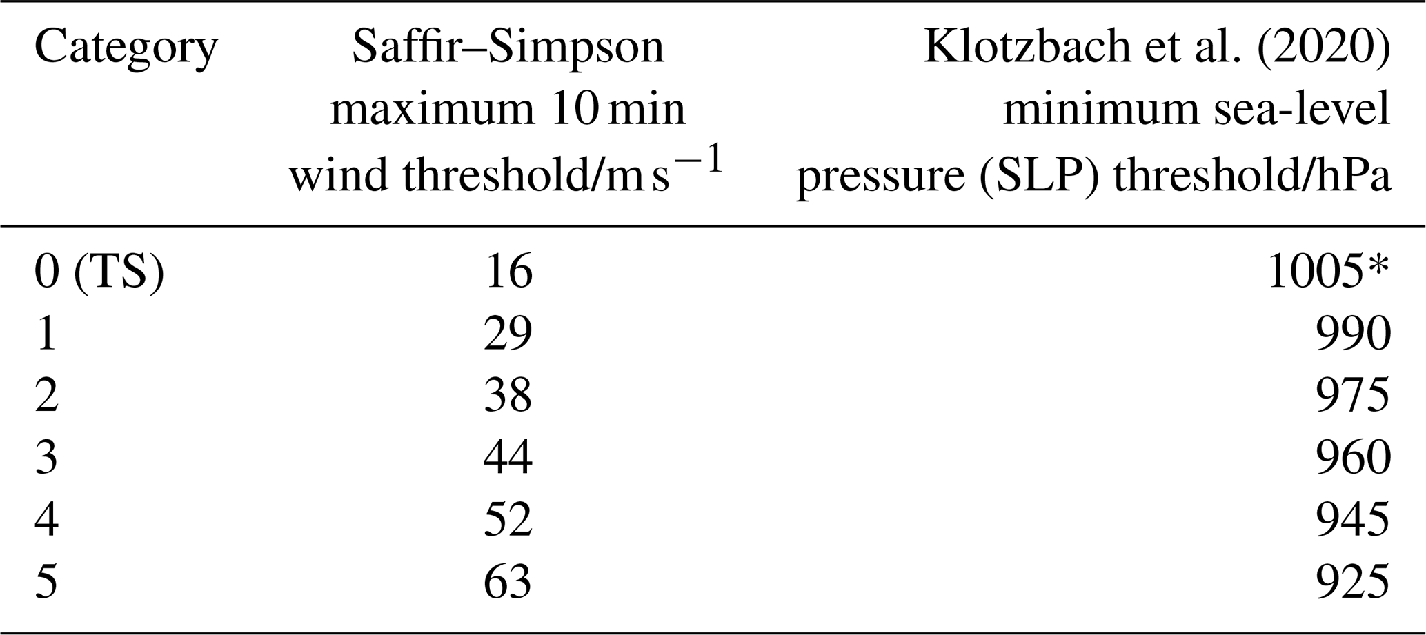
* This threshold is not in the original classification but has been derived by us using the same method.
Our analysis combines resources available for both the database of observed TCs, namely IBTrACS (Knapp et al., 2010) and the ERA5 reanalysis (Hersbach et al., 2020). Before describing these two datasets in detail, we first highlight our procedure to classify TCs according to their intensities. We next describe the specifics of the four trackers we compare in this paper, and explain our track-matching method.
2.1 Tropical cyclone (TC) intensities and classification
The TCs are commonly classified on the Saffir–Simpson Hurricane Scale (SSHS) with the peak 1 min near-surface wind (generally at 10 m above the surface). This is different from the World Meteorological Organization (WMO) standard to report the 10 min near-surface sustained wind u10. For that reason, we have chosen to systematically convert 1 min sustained winds to 10 min sustained winds. To do so, we applied the 1.12 coefficient provided by the IBTrACS documentation (Knapp et al., 2010), although we note there are some ambiguities in the precise value one should use for that purpose (Harper et al., 2010). As a result, u10 must exceed 29 m s−1 for a given structure to be classified as a TC, while tropical storms (TS) are defined as storms for which . The threshold values of u10 for each TC category are reported in Table 1.
In the present paper, we will evaluate TC intensities using their minimum SLP. As discussed in the literature in the past few years, the rationale behind this practice is 2-fold. First, minimum SLP is easier to measure than u10 (Klotzbach et al., 2020), thereby reducing the uncertainty associated with its evaluation. It is also uniformly defined among the different forecast agencies (Knapp et al., 2010), thereby removing the uncertainties associated with the conversion between winds obtained for different averaging periods such as described above. In addition, models tend to be able to reproduce the observed range of the minimum SLP of TCs but fail to simulate the largest wind speeds (Knutson et al., 2015; Chavas et al., 2017). The minimum SLP is a more reliable indicator of TC intensities than wind speeds. This is true in models, but also for ERA5, as recently shown by Zarzycki et al. (2021). Finally, and even if we do not tackle TC damage in this study, it has also been argued that minimum SLP is a better predictor of TC damage than maximum wind speed (Klotzbach et al., 2020).
Simpson and Saffir (1974) provided a version of the SSHS categorization in terms of pressure, but it does not preserve the proportion in categories of the wind scale. Therefore, we rather use the classification from Klotzbach et al. (2020) to compute TC intensity categories. It is reported in Table 1 for completeness.
2.2 Datasets
2.2.1 IBTrACS
The IBTrACS (Knapp et al., 2010) version 4 is the most comprehensive database of observed TCs. We used the “since 1980” subset in the present paper (Knapp et al., 2018). It combines data provided by TC centers of WMO, namely the Regional Specialized Meteorological Centers (RSMCs) and Tropical Cyclone Warning Centers (TCWCs), as well as non-WMO centers, such as the China Meteorological Administration, the Hong Kong Observatory, and the Joint Typhoon Warning Center. Since IBTrACS sources are so diverse, the database is heterogeneous and requires careful treatment before one can safely use it. The steps we followed are summarized below and detailed in a workflow chart (Fig. B1).
This study considers the cyclonic seasons from 1980 to 2019 in the Northern Hemisphere (NH, 40 seasons) and from 1981 to 2019 in the Southern Hemisphere (SH, 39 seasons). We removed seasons after 2019 because they contain provisional tracks. We also filtered out all tracks labeled as “spur” since they correspond to “usually short-lived tracks associated with main track and often represent alternate positions at the beginning of a system [or] actual system interactions”1. In the remaining tracks, we only kept 6-hourly time steps for consistency with ERA5. Winds and sea-level pressure (SLP) data were retrieved when available, prioritizing the WMO center responsible for the relevant region. Tracks lacking wind data (0.5 % of all tracks) were dropped. Tracks lacking SLP data (7 % of TS intensity tracks) were kept but not be included in those parts of the analysis for which storm intensities are needed. Finally, we removed tracks that do not reach the TS stage (16 m s−1) and those that last less than 1 d.
Hereafter, our selection of IBTrACS data will be referred to as IB-TS. We also define IB-TC as the subset of IB-TS tracks that reached the TC intensity (). IB-TS (resp. IB-TC) contains 3519 (resp. 1938) tracks.
2.2.2 ERA5
We retrieved data from the fifth generation of ECMWF Reanalysis (ERA5, Hersbach et al., 2020). Hourly estimates of atmospheric variables are provided by ERA5 on a grid with 0.25∘ horizontal resolution from 1979 to the present day. For the purpose of this paper, we only used 6-hourly data from 1980 to 2019 (as in IBTrACS). We made the choice of using 6-hourly data, considering our final objective, which is to use the trackers on simulations. In simulations, as is customary, we only have 6-hourly data available. However, we checked that the difference it makes is unimportant by running part of the tracking on 1-hourly data.
Unlike other reanalyses such as JRA-55 or NCEP-CFSR, ERA5 does not perform any specific assimilation for TCs (Hodges et al., 2017). Nevertheless, ERA5 has recently been assessed as having similar performances as JRA-55 or NCEP-CFSR for a range of metrics (Zarzycki et al., 2021; Roberts et al., 2020a). These results motivated our choice to use ERA5 as a test bed to benchmark the detection skills of the four different TC trackers we will now describe.
2.3 TC trackers
In Table B1 we provide a synthesis table of the trackers' criteria and thresholds presented below.
2.3.1 TempestExtremes
TempestExtremes (see https://climate.ucdavis.edu/tempestextremes.php, last access: 22 August 2022) has been developed by Ullrich and Zarzycki (2017) as a command-line software enabling a fast and versatile implementation of TC trackers.
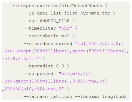
For the tracking of pointwise features, such as TCs, it provides two functions: (i) DetectNodes finds candidates “nodes” corresponding to local extrema of a given variable, and optionally satisfying a set of additional criteria (closed-contours, thresholds); and (ii) StitchNodes links candidates within a given distance of one another into a track. In this paper, we use TempestExtremes to implement two vastly different TC trackers, UZ and OWZ, respectively described by Ullrich et al. (2021) and Tory et al. (2013c). We describe both algorithms below and provide the associated codes in Appendix C.
2.3.2 UZ algorithm
We implemented the physics-based UZ algorithm in TempestExtremes as described by Ullrich et al. (2021). The thresholds were calibrated by Zarzycki and Ullrich (2017) using sensitivity analysis to several metrics and the data of four reanalysis products. This tracker was referred to as “TempestExtremes” in Roberts et al. (2020a, b) but we prefer to distinguish between the framework and the tracker formulation itself.
Candidate detection. The first step consists in finding the local minima of SLP. It defines a series of candidate points. In a second step, only those candidates that verify the following two closed-contour criteria are retained:
- i.
SLP must increase by 200 Pa over a distance of 5.5∘ great-circle distance (GCD) from the candidate point;
- ii.
Z300−500 – the geopotential thickness between 300 and 500 hPa – must decrease by 58.8 m2 s−2 over a distance of 6.5∘ GCD, using the maximum value of Z300−500 within 1∘ GCD of the minimum SLP as a reference.
Criterion (i) ensures that the low-pressure region is of sufficient magnitude and coherent. Criterion (ii) verifies that there is an upper-level warm core associated with the local depression. Finally, candidates for which a stronger SLP minimum exists within 6∘ GCD are eliminated.
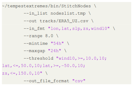
Stitching TC tracks. Consecutive candidates are linked together if they lie within 8∘ GCD of one another. A maximum 24 h gap is allowed in a track, and tracks must last for at least 54 h. Ten 6-hourly time steps (54 h) must also verify the following additional thresholds: , ∘, zsurf≤150 m, where ϕ and z stand for the latitude and the altitude, respectively. They respectively ensure that the track is of sufficient intensity, located close enough to the Equator, and spends a significant fraction of its lifetime over oceans.
2.3.3 OWZ algorithm
The OWZ algorithm, presented in Tory et al. (2013c) and assessed using ERA-Interim data by Bell et al. (2018) is based on evaluating the eponymous Obuko-Weiss-Zeta (OWZ) quantity, defined according to
where η is the absolute vorticity, the sum of the relative vorticity ζ and the coriolis parameter f, and OWnorm stands for the normalized Obuko-Weiss parameter:
in which E and F are the stretching and the shearing deformation, respectively and are given by
Candidate detection. Our implementation of OWZ in TempestExtremes first identifies local maxima of OWZ at 850 hPa. Candidates for which a stronger OWZ maximum exists within 5∘ GCD are eliminated. Next, only those candidates that satisfy the following six conditions within a distance of 2∘ GCD of that maximum are retained (with r and q being the relative and specific humidity, respectively, and vws denotes the vertical wind shear between 200 and 850 hPa):
Stitching TC tracks. Consecutive TC points are stitched together when they lie within a maximum distance of 5∘ GCD from one another, allowing for a maximum 24 h gap. Additional core thresholds must be reached for at least 9 time-steps (48 h):
Finally, tracks that do not reach TS intensity () for at least 1 time step are filtered out.
Due to the specifics of the TempestExtremes framework, we note that our implementation differs slightly from the original algorithm described by Tory et al. (2013c). These modifications, along with the results of a sensitivity study justifying our choices for rthreshold and rrange, are further discussed in Appendix C.
2.3.4 TRACK algorithm
TRACK derives from an extra-tropical cyclone (ETC) tracking algorithm (Hodges, 1994). It is versatile and has since been used to study many types of weather systems, including the detection and tracking of TCs (Bengtsson et al., 2007; Hodges et al., 2017; Roberts et al., 2020a). The rationale behind TRACK is different from the previously described trackers: because it aims to track all vorticity perturbations, it does not embed any warm-core criterion in its initial fundamental detection. The TC selection, including the warm core test, is only performed in the last step, independently of the tracking. In the present paper, we used the database of trajectories detected by TRACK in ERA5 that was recently published by Roberts et al. (2020a) without any modification. For completeness, we detail below the thresholds used in that case.
The algorithm is based on ζT63(P) which is the relative vorticity at pressure level P, spectrally filtered to retain total wavenumbers 6–63 only, as well as its vertical average from 850 to 600 hPa, hereafter referred to as . Local extrema of are detected and the ones for which define a series of candidate points. Neighboring candidates are then stitched together by minimizing a cost function for track smoothness (Hodges, 1995, 1999). The tracks so obtained must last for at least 2 d and start between 30∘ S and 30∘ N.
The presence of a warm core is diagnosed according to the following criteria that must be satisfied for at least 1 d over the ocean:
-
.
-
.
-
A local maximum of ζT63(P) exists at each pressure level.
2.3.5 CNRM algorithm
The CNRM algorithm was developed by Chauvin et al. (2006), and later used in Chauvin et al. (2020) and Cattiaux et al. (2020).
Candidate points are first tracked with the following criteria:
-
The SLP displays a local minimum which defines the center of the system.
-
The 850 hPa relative vorticity is larger than s−1.
-
The 850 hPa wind intensity is larger than 5 m s−1.
-
The sum of the temperature anomalies averaged over the 700, 500, 300 hPa pressure levels is larger than 1 K.
-
The difference between the 850 and 300 hPa temperature anomalies is smaller than 1 K.
-
The difference between the 300 and 850 hPa wind intensity is smaller than 5 m s−1.
This detection step is followed by a stitching procedure adapted from Hodges (1994) and detailed in Ayrault (1998). Tracks shorter than 1 d are eliminated. Once TC tracks are obtained, a relaxation step is performed to complete the track life cycle and to detect tracks that were cut into two or more pieces (for example, because of a temporary weakening). This relaxation step is done with a 850 hPa relative vorticity threshold equal to s−1.
2.4 Tracks matching
When using reanalysis products like ERA5, detected tracks can tentatively be associated with observed tracks (Murakami, 2014; Hodges et al., 2017; Ullrich et al., 2021). We derived the following matching algorithm: consider the case of a given detected track D composed of n points () defined at times (). The observations O consist of a database of tracks and can be seen as a collection of points at given times. For each point di(ti) of track D, we associated those points of O at time ti that are located closer than 300 km from the point di. Of course, it is possible that such points do not exist in O. The subset of points of O that have been associated with any point in D is denoted as OD−paired. It is composed of elements. There are three possibilities:
-
: None of the points of D has been paired to a point in O and D is considered to be an FA.
-
and all the points in OD−paired belong to the same track DO in O: DO is considered to be the match of D.
-
and the points in OD−paired belong to more than one track in O: the observed track having the largest number of points paired with D is considered the match of D.
After this matching is completed for all detected tracks, a final treatment is performed: if an observed track is paired with two or more detected tracks, these detected tracks are merged into a single track. Such cases arise when the detected track corresponds to different parts of the same observed tracks and occur when, for example, the TC temporarily weakened while going over an island before strengthening again. In Appendix D, we present a rapid analysis that validates our method.
This matching procedure enables us to label tracks as “Hits” (H), “Misses” (M), and “False Alarms” (FAs). Hits are tracks present in IB-TS and detected in ERA5. Misses are tracks present in IB-TS that were not detected in ERA5. False Alarms are tracks detected in ERA5 that do not correspond to any track in IB-TS. We then used this labeling to define two detection skills metrics, the Probability of Detection (POD, sometimes also presented as HR for “Hit Rate”) and the False Alarm Rate (FAR):
We used Eqs. (3) and (4) to calculate the POD and FAR of the four trackers with respect to IB-TS. For UZ, we found a POD of 75 % and an FAR equal to 18 %. These values are almost identical to Zarzycki et al. (2021), who report 78 % and 14 % for their POD and FAR, respectively. Subtle differences in the pre-processing of the IBTrACS data account for this difference (Colin Zarzycki,, personal communication, 2022) but the fact that both PODs and FARs are almost identical validates our implementation of that tracker. For TRACK, we found a POD of 85 % and a FAR equal to 50 %. Both scores are comparable to the values reported by Hodges et al. (2017), who applied TRACK to other reanalyses. We note that the POD we report here is on the higher end of the values found by Hodges et al. (2017), which is consistent with our more restrictive filtering of IBTrACS than Hodges et al. (2017). The OWZ and CNRM trackers display PODs similar to UZ, but their FARs are more heterogeneous and amount to 28 % for OWZ and 60 % for the CNRM tracker.
Overall, the results demonstrate that all trackers can capture most of the observed TCs. Although this is satisfying, we note that a given tracker can miss up to one-fourth of the existing tracks. In addition, as stated above, the FARs are more heterogeneous, and FAs can account for more than half of the detected trajectories. These two caveats call for a better understanding of the properties of both populations. This is the purpose of the following section.
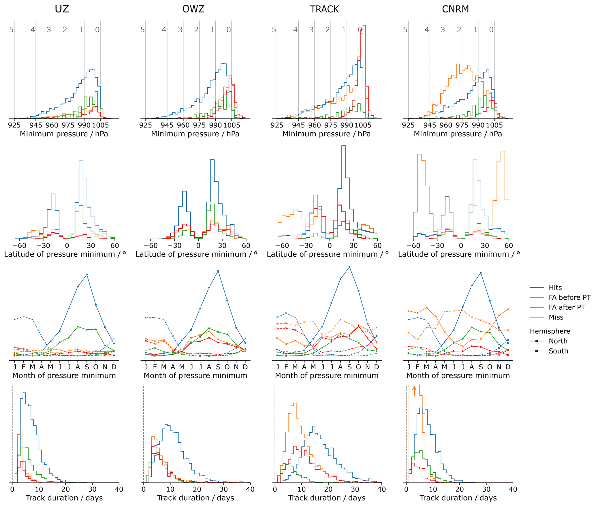
Figure 1Histograms representing the properties of the Hits, the Misses, and the False Alarm (FA) tracks for each tracking algorithm. From left to right, the columns correspond to UZ, OWZ, TRACK, and the CNRM tracker, respectively. The rows correspond from top to bottom to the minimum sea-level pressure (SLP, with the storm categories as defined according to Table 1 shown with vertical gray lines), the latitude at which that value is reached, the month at which that value is reached (solid line in the Northern Hemisphere, and dashed line in the Southern Hemisphere), and finally the track duration. The blue and green colors correspond to the Hits and the Misses, respectively, for all plots. Raw FAs are shown in orange while we plot the FAs that remain after the post-treatment in red (see Sect. 3 for details). The histograms display counts that have not been normalized. Hence, the area under each curve is proportional to the number of tracks in each ensemble.
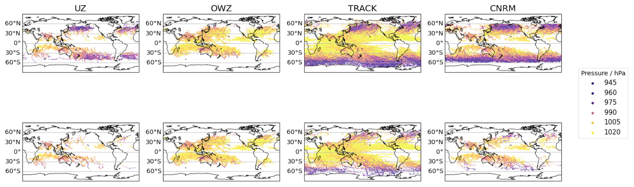
Figure 2Top row: maps of the FA tracks color-coded according to their intensity in terms of pressure. The different columns each correspond to a different tracker. Bottom row: same as the top row, but after the sub-tropical jet (STJ) post-treatment has been applied (see Sect. 3).
3.1 Missing tracks and false alarm (FA) properties
Figure 1 reports several diagnostics that characterize the different populations (hits, misses, and FAs) detected in ERA5 by the trackers.
For practical purposes, we use the hits (blue color in Fig. 1) as a reference against which to compare these diagnostics. The TC intensity distribution (first row) and seasonal cycle (third row) are similar across all trackers. The seasonal cycle is the same as in the observations, but the intensity distribution is underestimated (see Sect. 4.4). We find some differences in the latitude at which the SLP minima are reached (second row). The CNRM tracker distribution features secondary maxima in midlatitudes in both hemispheres that are absent in UZ and OWZ and only barely visible in TRACK (particularly in the Southern Hemisphere). These tracks correspond to TCs that reached their maximum intensities after a post-tropical transition. The lifetimes of hits (fourth row) also vary with trackers: UZ and the CNRM display the shortest tracks with a distribution that peaks between 5 and 10 d, followed by OWZ with storm durations peaking at 10 d, while TRACK tracks typically last for 15 d. We will revisit these properties in Sect. 4.3.
Missing tracks (green color in Fig. 1) correspond to TS or TCs that were observed and are reported in the IB-TS database but that a given tracker did not find in ERA5. They typically consist of weak (first row), tropical (second row), and short-lived (fourth row) perturbations for which the amplitude is probably not strong enough to exceed the detection thresholds for a long-enough time2. This is why TRACK, with its relatively soft criteria, misses half as many tracks as the other trackers. We also note that the latitudinal distribution of missed tracks (second row) is skewed in favor of the Northern Hemisphere, a property they share with the population of hits. Because they are observed as a tropical storm, missing tracks are more numerous during the TC season of their hemisphere (third row). To conclude, the missed trajectories seem to correspond to the weak tail of the distribution of hit trajectories. Our description of missing tracks is in agreement with Hodges et al. (2017).
The FAs (orange color in Fig. 1) correspond to perturbations detected in ERA5 by a given tracker for which no correspondence in IB-TS exists. The FA storms are not systematically weak and their intensity distributions vary across trackers (first row). The CNRM tracker shows the most extreme distribution of FAs, with a peak that corresponds to category 2 storms. By contrast, the OWZ distribution of FAs is strongly biased toward weak category 0 storms. The UZ and TRACK strength distributions of FAs simultaneously show weak storms along with a significant tail of strong storms – in the sense that the number of category 1 and 2 storms is not negligible compared to the number of category 0 storms. The second row of Fig. 1 suggests that these relatively strong disturbances correspond to ETCs. Indeed, the latitude distribution of the minimum SLP value shows two peaks at midlatitudes for UZ, TRACK, and the CNRM tracker. For the latter, these peaks even exceed the subtropical peaks associated with the hits. In agreement with that hypothesis, the seasonality of FAs in UZ, TRACK, and CNRM shows that there is an important number of storms detected during the winter season of each hemisphere, i.e., precisely when ETCs are numerous (Fig. 1, third row). By contrast, OWZ FAs occur during the TC season. For all trackers, the ratio of summer to winter FAs is consistent with the ratio of the peaks observed at tropical and midlatitudes in the latitudinal distribution of FAs: UZ and TRACK FAs have rather flat seasonal cycles, and the same number of tropical and extra-tropical FAs. The CNRM tracker has most of its FAs during winter at extra-tropical latitudes, and OWZ FAs mainly occur during the TC season at tropical latitudes. Finally, FAs are generally shorter events than hits (last row). The UZ and CNRM FAs tracks are the shortest and last less than 10 d. The longest tracks are the TRACK FAs and feature durations of up to a month. The OWZ FAs can last up to 20 d. Interestingly, Bell et al. (2018) also reported similarly long FAs while tracking TCs in ERA-Interim with OWZ. They were then able to associate the longest FAs with observed tropical disturbances that had been discarded from IBTrACS because they only retained storms of tropical intensity and stronger, as we did in this paper. Although we did not do the same exercise, in light of their results, it is likely that some of the FAs we report here also correspond to weak storms we excluded from IBTrACS.
We conclude that FAs belong to two categories: (i) strong extra-tropical and (ii) weak tropical storm. This conclusion is nicely illustrated and confirmed with the help of FA track maps (Fig. 2, top row): For UZ and the CRNM tracker, FA tracks correspond to intense storms (pink colors) that cluster beyond 30∘ latitude. On the other hand, OWZ FAs are located in the tropics and are weak disturbances (yellow colors). The TRACK FA tracks are of both types: many of them are strong extra-tropical storms, but there is also a large contingent of weak tracks.
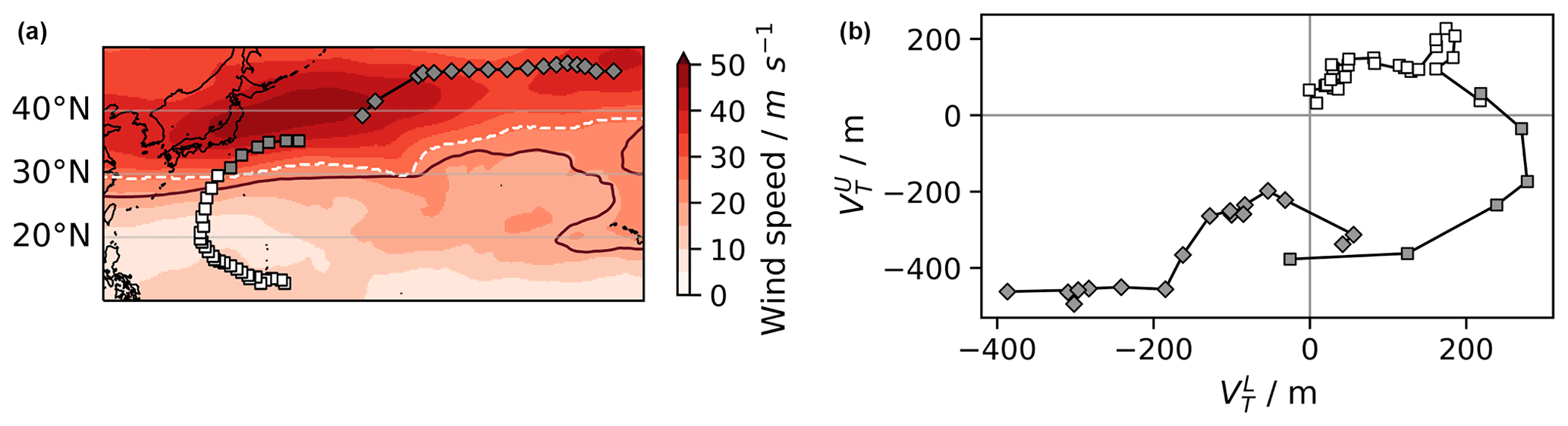
Figure 3Illustration of the post-treatment procedures of (a) STJ and (b) VTU. Panel (a) shows a close-up map of the western North Pacific (WNP). It displays two tracks detected by the UZ tracker that occurred simultaneously (represented using square and diamond symbols). Also shown are the 200 hPa horizontal wind speed (red shadings), the 15 zonal wind contour (dark red line) and the sub-tropical jet limit at that time as defined in Sect. 3.2 (dashed white line). Panel (b) displays both tracks in the Hart phase space diagram, also defined in Sect. 3.2. The track represented using square symbols on both panels features more than one point equatorward of the sub-tropical jet limit (a) and in the upper part of the Hart diagram (b). It is thus classified as a genuine TC according to both post-treatment methods. In fact, it corresponds to Typhoon Mac (1982) as found using the track-matching procedure described in Sect. 2.4. By contrast, the track represented with diamonds on both panels lies poleward of (a) the sub-tropical jet limit and (b) in the lower part of the Hart diagram. It is thus classified as an ETC according to both post-treatment methods. It was indeed classified as an FA according to the track matching algorithm. Finally, note that the gray points correspond to points that lie poleward of the sub-tropical jet limit and are therefore labeled as extra-tropical by the sub-tropical jet method.
3.2 Post-treatment: two methods
The discussion above identified two types of FAs: weak, short-lived TS and strong ETCs. It seems complicated to filter the weak and short-lived tracks because such a procedure would simultaneously remove many hits and significantly reduce the POD. For example, 24 % to 83 % of the tracks (for TRACK and UZ, respectively) with a minimum pressure larger than 1005 hPa are hits.
By contrast, ETCs are sufficiently different from genuine TCs to derive a discriminating method. We note that such an avenue for improvement has already been explored in the past. For example, based on the fact that ETCs preferentially develop in midlatitudes, some trackers use a fixed latitude criterion to filter out some of the tracks suspected to correspond to ETCs (see e.g., Table 1 in Chauvin et al., 2006). Such a simple criterion may not be elaborate enough, though. For example, it does not take into account the natural variability of the sub-tropical limit nor its potential poleward shift with climate change (Arias et al., 2021). In fact, the two trackers in this study that embed such a cut-off parameter (UZ and TRACK) still present a large number of extra-tropical tracks, suggesting that there is room for improvement. An alternative option is to rely on the structural differences between TCs and ETCs, for example, the nature – warm or cold – of their core.
In the following discussion, we develop and analyze the results and relative merits of both approaches. We propose two post-treatment methods inspired by the existing literature: (1) an adaptation of Bell et al. (2018) sub-tropical jet (STJ) cut-off, hereafter called the STJ method, and (2) an exploitation of Hart phase space diagram (Hart, 2003), hereafter called the VTU method.
The STJ method (see Fig. 3, left panel for a graphical illustration) is an environmental method that aims to establish an objective criterion to determine whether a given disturbance is located in the midlatitudes or the tropics. It is based on the large-scale wind field properties at 200 hPa. First, we apply a 30 d running mean on both wind components to remove the fast atmospheric synoptic activity. The sub-tropical jet is then defined as the region where the wind speed is larger than 25 m s−1 and the zonal wind u200 is larger than 15 m s−1. At each time step, we define the maximum tropical latitude for each longitude as the equatorward boundary of the sub-tropical jet. For those longitudes where no sub-tropical jet exists, the boundary latitude is linearly interpolated between the two closest longitudes with an existing sub-tropical jet. Any disturbance located poleward of that limit is assigned an extra-tropical label. We eventually filter out tracks that feature no or only one tropical point.
The VTU method (see Fig. 3, right panel for a graphical illustration) is a structural method that aims to establish an objective criterion to discriminate between TCs and ETCs. Here we use the Hart phase space diagram that plots storm trajectories in a 2D diagram based on measures of the storm thermal wind in the upper and lower troposphere, respectively denoted as and (Hart, 2003). We used the following relation to calculate :
where Ptop=300 hPa, Pbottom=600 hPa, , and . The ΔZ(P) denotes the maximum height perturbation on the isobaric surface of pressure P within a circle of a 500 km radius centered on the storm:
has a similar definition but with Ptop=600 hPa and Pbottom=900 hPa. As noted by Hart (2003), storm trajectories in the plane are enlightening as to the nature of the storm, and we have found that is a powerful discriminant between full-troposphere warm-core TCs and other structures. In practice, the VTU method consists of filtering out tracks for which is negative for all time steps.
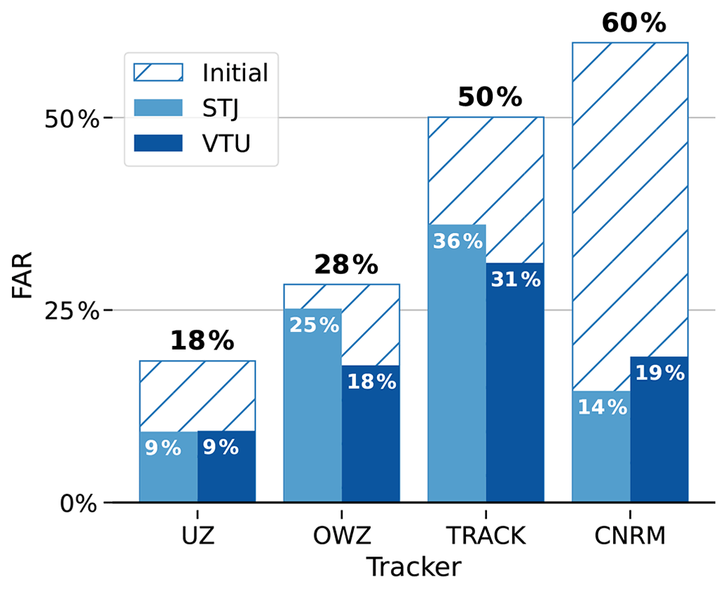
Figure 4FARs for each algorithm, before (hatched, black figures) and after (filled, white figures) post-treatment.
3.3 Post-treatment: the results
Both post-treatment schemes are effective at reducing FARs (see Fig. 4). The STJ method removes between 11 % and 76 % (for OWZ and CNRM, respectively) of FAs, while the corresponding reductions range from 37 % up to 68 % (for OWZ and CNRM, respectively) with the VTU method. The STJ reductions in FAR correspond to the proportion of extra-tropical FAs identified in Sect. 3.1: barely any in OWZ, about half in UZ and TRACK, and most in CNRM tracks.
In Fig. 1, we further compare the properties of the FAs before and after the STJ post-treatment, respectively with the orange and red distributions (The effects of the VTU method on the FA distributions are shown in Fig. B2 and are almost identical). The large amplitudes of the tail of strong storms and the secondary peaks at midlatitudes are significantly reduced for all trackers (first and second row). Both distributions are now similar to that of the hits. Furthermore, the seasonal cycle of the filtered FAs looks more similar to that displayed by actual TCs (third row). The visual inspection of STJ-filtered FA tracks (Fig. 2, second row) confirms these quantitative diagnostics and shows that the filtering procedure has dramatically reduced extra-tropical track frequencies. We conclude that the STJ method fulfills its goal of selectively removing ETC tracks.
The FARs after post-treatment are similar with both methods. They range from 9 % up to 36 % for the STJ method and from 9 % up to 31 % for the VTU method (see also Table 2). However, OWZ seems to be an exception to that rule. While the STJ method leaves its FAR nearly unchanged, the VTU method succeeds in removing more than one-third of its FAs. This relatively poor performance of the STJ method at removing OWZ FAs was to be expected. As discussed above in Sect. 3.1, extra-tropical storms do not dominate its population of FAs, which rather appear to be composed mostly of weak short storms. This is most likely because OWZ already embeds a wind shear criterion in its formulation. It probably already detects the crossing of the sub-tropical jet, thereby reducing the interest of the STJ filtering method. By contrast, the better performance of the VTU method for that tracker suggests that it is more efficient at identifying weak/short FA tracks and makes it more interesting to use in combination with OWZ. Nevertheless, we note that our results are in agreement with Bell et al. (2018), who report a decrease of 2.5 % and 4.5 % of the total tracks in NH and SH, respectively, when they used an STJ-like criterion on ERA-Interim data. In our case, we found that the STJ post–treatment removes 4 % of all the OWZ tracks. The detection scores obtained for OWZ after the STJ post-treatment are also close to those obtained by Bell et al. (2018) with ERA-Interim, i.e., a 73 % POD and 19 % FAR.
As mentioned above, a desired property of any post-treatment procedure is to leave the POD unaltered. We found that the two methods display some differences (see Fig. 5). While the STJ method only reduces the POD by 1 % at most for all trackers, the VTU method has a larger impact: PODs decrease from 3 % (for TRACK) to 7 % (for the CNRM tracker). The VTU post-treatment even removes up to 4 % of TC-strength hits in UZ and CNRM. For this reason, we only present results obtained using the STJ method in the remainder of this paper. It does not mean that the VTU post-treatment should always be discarded. As opposed to the STJ method, it only requires information about the local and instantaneous properties of the flow. The VTU method is thus simpler to implement than the STJ method. This relative simplicity has a price to pay in terms of a modest decrease of PODs that one should be aware of.
In addition to filtering out ETCs, the post-treatment methods described above allow us to label extra-tropical points in the remaining tracks. These extra-tropical points are then excluded when computing the intensity statistics of the tracks (see Sect. 4). This “free bonus” of the post-treatment step removes potential biases in the metrics that would result from TC tracks that reach their maximum intensity after performing a post-tropical transition.
We now analyze the properties of the database of ERA5 tracks that we obtained after the post-treatment described above, focusing on the differences between trackers. We first revisit the detection skills of trackers (Sect. 4.1). We then discuss the sensitivity of the metrics introduced by Zarzycki et al. (2021) in Sect. 4.2 and thereafter relate these sensitivities to the different tracks' duration as captured by the four trackers (Sect. 4.3) and to the intensity distribution of the reanalyzed storms in ERA5 (Sect. 4.4).
Table 2Probability of detection (POD) and false alarm rate (FAR) of the four trackers used in this paper with respect to IB-TS.
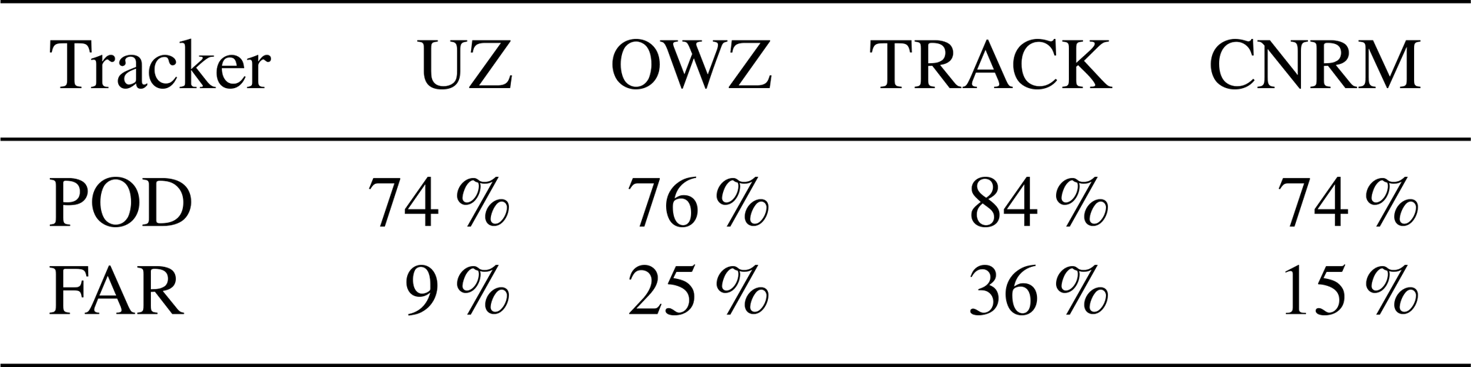
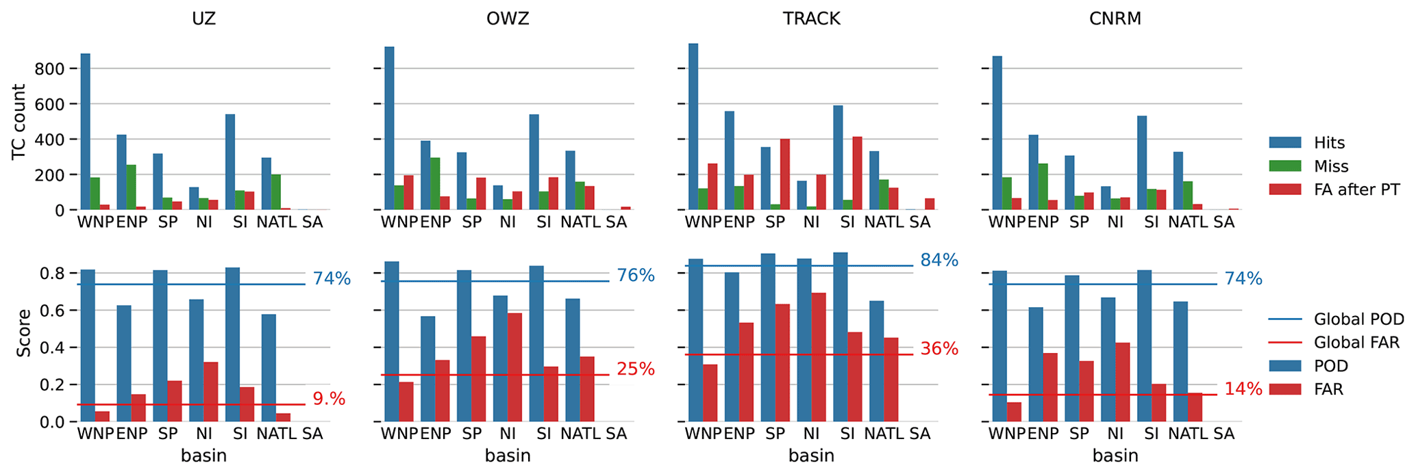
Figure 5Upper panel: Hits, misses and FA total numbers per oceanic basin. From left to right, the different panels correspond to UZ, OWZ, TRACK and the CNRM tracker, respectively. Lower panel: POD and FAR for each tracker in each basin (bars) compared to the global mean (lines). Basin abbreviations are defined as follows: western North Pacific (WNP), eastern North Pacific (ENP), South Pacific (SP), North Indian (NI), South Indian (SI), North ATLantic (NATL), and South Atlantic (SA).
4.1 Trackers' detection skills
For completeness Table 2 summarizes the filtered trackers' detection skills that were extensively discussed in the previous section. The PODs are almost unchanged compared to the values discussed in Sect. 3 before post-treatment, and the FARs are as shown in Fig. 4 for the STJ method. Overall, these numbers illustrate the trade-off between FAs and misses: improvements of the POD tend to occur at the cost of an increase in the FAR.
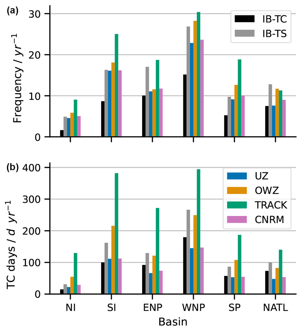
However, these numbers are global averages and hide a significant regional variability. This variability is illustrated in Fig. 5 (top row), which decomposes the numbers of hits, misses, and FAs by oceanic basins3. First, we note that the hits' geographical distribution is similar across trackers: they are more numerous in the western North Pacific (WNP), followed by the South Indian (SI), the eastern North Pacific (ENP), and finally the South Pacific (SP) and North Atlantic (NATL) which features almost the same number of TCs. The geographical distribution of misses is not identical to that of the hits and varies among trackers. This variability translates into POD values than can strongly deviate from the mean (Fig. 5, bottom row). For example, the POD in the NATL is smaller than the global average by 10 % for all trackers and only reaches 58 % for UZ. Misses are also more numerous in the ENP, although with contrasted results among trackers: while UZ, OWZ, and CNRM PODs roughly equal 60 %, it amounts to 80 % for TRACK, i.e., close to its global average. We find similar figures for North Indian (NI). These problems are balanced by POD scores that are systematically larger than the global averages for WNP, SP, and SI oceans, where the PODs are larger than 80 %. With almost two-thirds of the world's TCs occurring in the WNP and SI oceans, these two basins largely account for the global averages reported in Table 2.
Similarly, the geographical distribution of FAs does not necessarily follow that of the hits and is heavily weighted by the WNP value. In this basin, the FAR is equal to 8 % and 10 % for UZ and the CNRM trackers, respectively, and largely explains the low FARs for these two trackers. It amounts to 20 % and 30 % for OWZ and TRACK, also reflecting their global average values. In many of the other basins, FARs are much worse than their global averages and often exceed 40 %. This is particularly true for the southern oceanic basins and NI ocean. In fact, regional FARs smaller than the global mean are an exception rather than the rule.
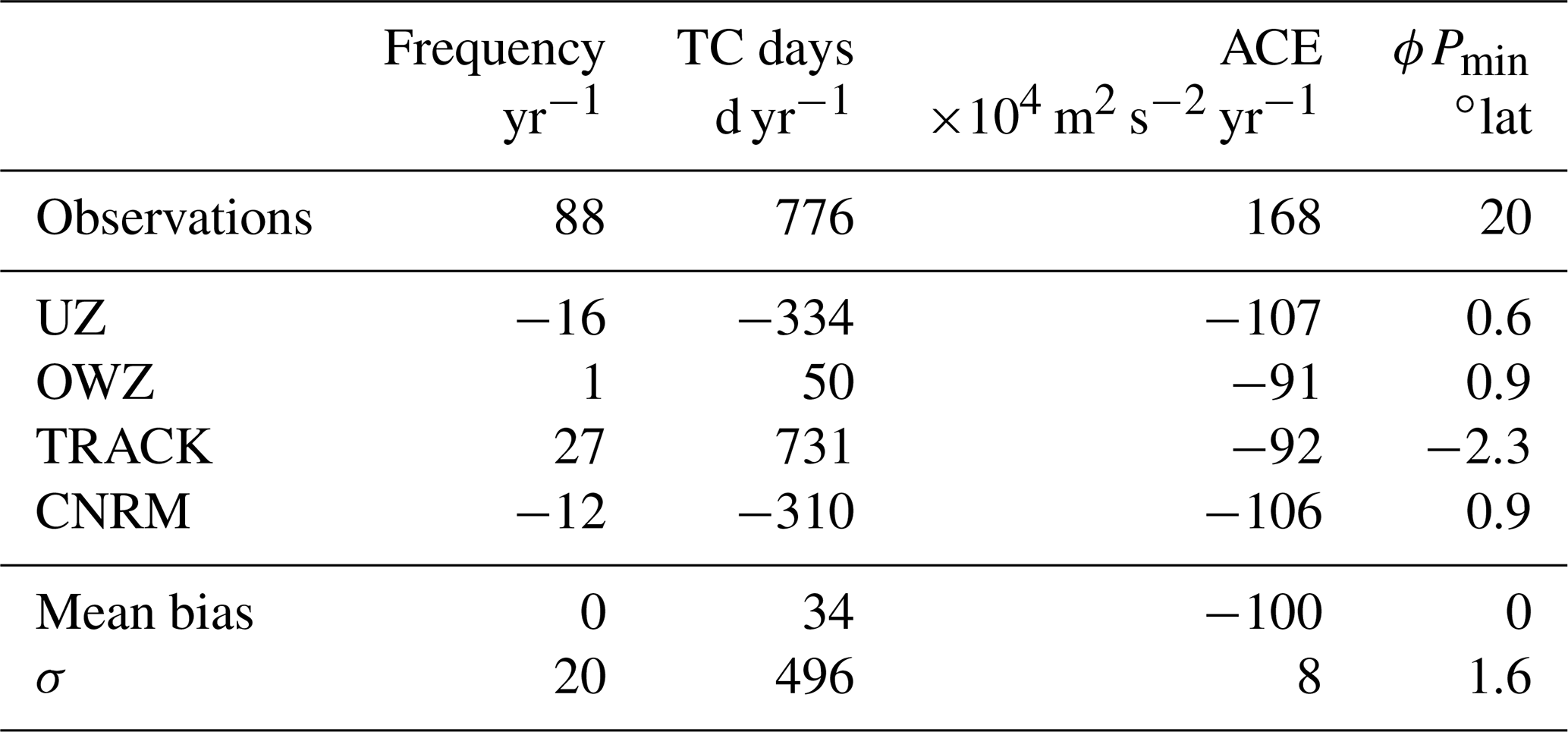
Table 3Frequency, TC days, ACE and latitude of minimum pressure () in the observations, and bias in ERA5 depending on the tracker used. The last two lines show the mean and the standard deviation of the bias with regard to the trackers.
4.2 Metrics sensitivity
We now take a different view of assessing the properties of the detected tracks as an ensemble composed of the hits and FAs aggregated together. We compare them with the properties of the observed tracks as derived from IBTrACS. Such an approach would be more appropriate when using trackers to evaluate model results as opposed to reanalysis for which detection scores can be calculated.
To do so, Zarzycki et al. (2021) suggested using a series of standard metrics as a means to evaluate the performance of a system in simulating tropical storms against an observed reference. Using the UZ tracker (albeit without the post-treatment method described above), they applied it to several reanalysis products. Here, we take a complementary viewpoint and use a subset of their metrics to evaluate the performances of several trackers against a single reanalysis product. Table 3 reports the bias we measured for each of these metrics and for each of the trackers with respect to IB-TS.
The global storm frequencies – i.e., the total number of storms detected per year – vary among trackers and reflect their different sensitivities: UZ and the CNRM tracker are the most selective and display a negative bias. TRACK is the most sensitive tracker and has a positive bias. The behavior of OWZ is intermediate and features a very small bias. Perhaps more important than their absolute value is the fact that the standard deviation of biases (σ=20 yr−1) amounts to more than 20 % of the observed track frequency. It is also comparable to the dispersion of track frequencies of 18.3 yr−1 reported by Zarzycki et al. (2021) in their analysis of a series of reanalysis products with a single tracker. This comparison indicates that uncertainties associated with using a single reanalysis product are as large as those associated with using a single tracker.
Zarzycki and Ullrich (2017) and Zarzycki et al. (2021) advocate using more integrated metrics, such as the total number of days featuring TCs, also referred to as TC days. We recover biases of the same sign as that of the frequencies for that metric. For UZ, the bias is very different in both its sign and amplitude from the value reported by Zarzycki et al. (2021). This is because we consider the entire trajectories reported in IBTrACS, while Zarzycki et al. (2021) only included storms of TS strength (i.e., with u10>16 m s−1). The observed number of TC days that they calculated is thus smaller than the values we report in Table 3, explaining the differences between the biases. Even if the number of TC days is an integrated metric, its scatter among the different trackers is even larger than found for the frequencies and amounts to 63 % of the IB-TS value. This large scatter is due to the fact that TC days multiplies TC frequencies with track duration. As already discussed in Sect. 3.1, the latter is variable among trackers, and that variability is positively correlated with trackers' sensitivities: tracks durations increase for sensitive trackers. We will revisit that aspect in Sect. 4.3.
As already mentioned in Sect. 4.1, there is significant regional variability of the POD and FAR. This is also the case for the aggregated catalog (hits plus FAs), as illustrated in Fig. 6 (top row), where we also compare our results with both IB-TS and IB-TC. First, we note that TCs' frequency biases with respect to IB-TC are positive for all trackers and all basins. The comparison with IB-TS is more variable. We recover the negative biases in frequencies of UZ and CNRM for all basins, although with different amplitudes: it is large in the ENP but nearly vanishes in the SI and SP oceans. Similarly, OWZ features smaller biases but with different signs depending on the basins and occasionally displays large values, for example, for the ENP. The TRACK biases also tend to be positive and large, in line with the global positive bias, except for NATL. The low POD we already noticed in that basin is not compensated by FAR, and the number of detected tracks remains smaller than observed, even for that sensitive tracker. Surprisingly, this is also the only basin where OWZ outnumbers TRACK. Concerning TC days, the geographical distribution (Fig. 6, bottom row) visually confirms the larger scatter for that metric than for the frequencies. However, the biases with respect to IB-TS appears to be more homogeneous, with large negative biases obtained for UZ and CNRM, a small bias for OWZ and large positive biases for TRACK, occasionally showing TC days larger by more than a factor of 2 compared to the observed value, as is the case for example in the SI and SP oceans and for ENP. This consistency between the regional and global biases also manifests itself in the good spatial correlations between the observed and detected catalogs. In agreement with Zarzycki et al. (2021), we indeed found a correlation coefficient of 0.97 between UZ and IB-TS, while we obtained similar albeit slightly smaller values of 0.93, 0.85 and 0.96 for OWZ, TRACK and the CNRM, respectively.
Table 3 also reports the values of the accumulated cyclone energy (ACE), which is a measure of the storms' maximum kinetic energy:
where is the maximum 10 m wind speed reached by each of the tracks and the sum is over the total number of detected or observed tracks. In agreement with Zarzycki et al. (2021), the ACE bias is negative for UZ as well as for the other trackers. The values are also much more homogeneous because ACE is heavily weighted by the more powerful TCs for which the different trackers agree. We will revisit that point in Sect. 4.4.
Finally, the latitudes of minimum pressure is well represented in ERA5 (Table 3, last column). The UZ bias is smaller than reported by Zarzycki et al. (2021) and the actual value of is closer to the observed value. This reduction is a consequence of the removal of extra-tropical tracks by the post-treatment. Before filtering, we indeed found a bias in equal to 3.5∘. This is also in agreement with the interpretation of Hodges et al. (2017), who found positive biases for a large number of reanalyses when using TRACK. In our case, we note that TRACK is the only tracker with a negative bias, a fact we attribute to the post–treatment as well, and to the large number of FAs. The latter are mostly composed of short and weak storms that preferentially develop equatorward of the population of hits.
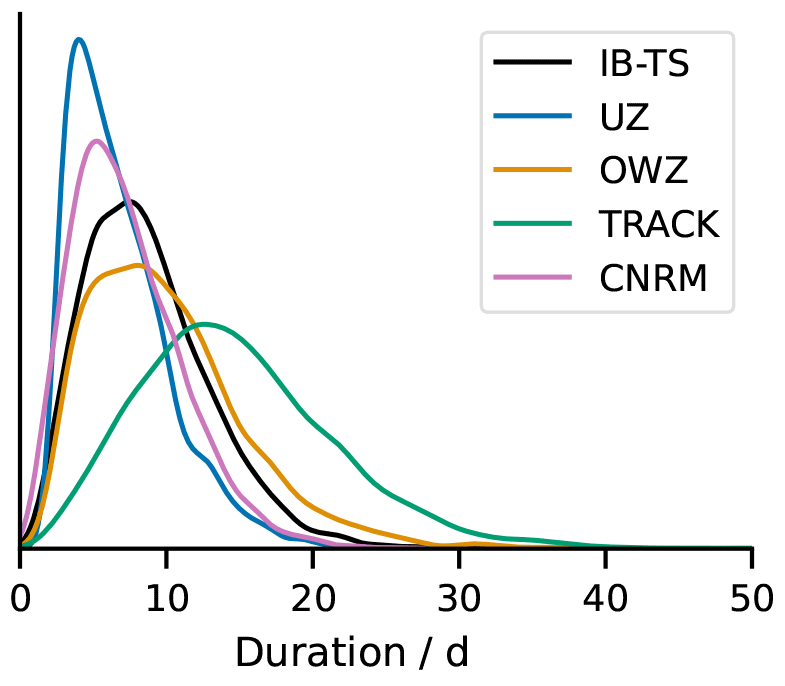
Figure 7Normalized distribution of track duration for all tracks detected by each tracker, after the STJ filtering, compared to IB-TS.

Figure 8Delay between the first (last) detection by each of the trackers and the first (last) record for the corresponding storm in IBTrACS is presented on the left (right) panel. The different colors correspond to different basins, whose abbreviations are as defined in Fig. 5. Boxplots display 25th, 50th, and 75th percentiles, whiskers display 10th and 90th percentiles, outliers are not shown.
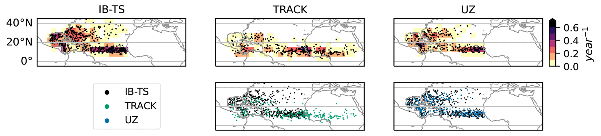
Figure 9First observed/detected points in IB-TS, TRACK and UZ. Top row shows the first points along with the corresponding density. Bottom row overlays IB-TS tracks' first point with ERA5 tracks' first point as detected tracks by TRACK (second column) and UZ (third column).
4.3 Track duration
In Sect. 4.2, we argued that the increased scatter for TC days compared to that of the frequencies was due to the differing track durations detected by the different trackers (see also Sect. 3.1, which highlights that issue for the hits). Figure 7 shows that this is indeed the case: track durations are ranked according to the tracker sensitivity, and the corresponding distributions are found to peak at 5, 6, 8, and 12 d for UZ, the CNRM, OWZ, and TRACK, respectively. Hodges et al. (2017) already showed such long TRACK storm durations for other reanalyses products. We find here that they are also longer than IB-TS tracks. The durations of OWZ tracks are closest to the observations, while UZ and CNRM tracks are shorter than IB-TS tracks.
To illustrate that point further, we can compare the first and final dates of detected and observed tracks (Fig. 8). This comparison demonstrates that durations of tracks are homogeneous across oceanic basins. The only exception may be the WNP, where the results suggest a tendency for UZ and the CNRM tracker to detect tracks later than other oceanic basins. In general, TRACK detects the most extended TC life cycle: 50 % of its tracks start 4 d or more before the first IBTrACS record and terminate 2 d or more after the last IBTrACS record. Figure 8 also shows that three-quarters of OWZ tracks start before IBTrACS but present a reduced ability to follow a track after its recurvature. The UZ and CNRM tracks are very similar to the IBTrACS ones, although slightly shorter in general. These results may sound surprising at first because they appear to disagree with Fig. 7 where we found that OWZ tracks correspond to IB-TS while UZ and CNRM tracks were significantly shorter. The difference is due to the FAs: necessarily, Fig. 8 is restricted to matching tracks, i.e., to the hits. As discussed above, FAs are mainly composed of short and weak tracks, which reduce the mean duration of the trackers' trajectories, explaining the differences between the two figures. Interestingly, we note that the two dynamics-based trackers in our study share the capacity to detect the storms early in their development.
One can use the ability of TRACK – and, to a lesser extent, OWZ – to detect storm tracks early in their life cycle to study the genesis locations of TCs. For example, in the NATL, although the exact role of African easterly waves (AEW) is still debated (Patricola et al., 2018), there is a correlation between AEW and cyclogenesis (Landsea, 1993; Avila et al., 2000). It is therefore interesting to be able to probe the early parts of TCs life cycles. In IBTrACS, the first reported point of TC tracks tends to be located in the eastern central Atlantic ocean, in agreement with the tracks detected in ERA5 by UZ (Fig. 9, left and right panels). By contrast, TRACK's genesis locations extend further east and well over the African continent (Fig. 9, middle panel), i.e., well into the region where AEWs develop. These differences in genesis locations illustrate TRACK's ability to follow the vorticity perturbations that later transform into genuine TCs from very early on, and potentially to associate these early perturbations with known atmospheric phenomena. In this regard, OWZ is a middle ground between TRACK and UZ (Fig. 8, left panel), and is able to find some precursors over land (Fig. B3). The CNRM tracker is very similar to UZ, except it catches some precursors over land, probably because of its specific relaxation step that only takes vorticity into account. This property of TRACK and OWZ opens the way for studying the correlation between NATL TC genesis and AEW in ERA5, in the spirit of studies such as conducted by Thorncroft and Hodges (2001); Hopsch et al. (2007) and Duvel (2021). It would be interesting to further exploit that property by performing similar studies of TC precursors in other oceanic basins systematically, especially in the context where some of the uncertainty related to climate-change projections of TC activity is due to the lack of understanding of TC seeding and whether it is a driver of the natural variability of TCs (Vecchi et al., 2019).
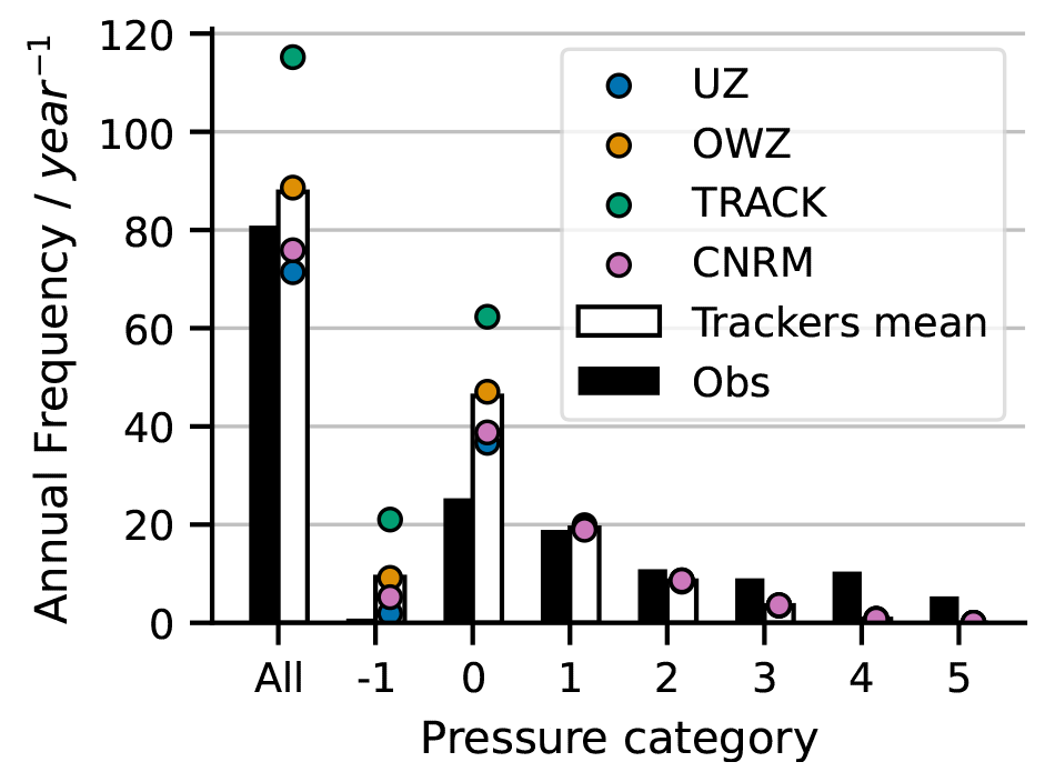
Figure 10Annual frequency depending on the pressure category in IBTrACS (black bars), and as found by each tracker in ERA5. The colored dots show the result of each tracker and the mean is represented with the white bar. The −1 category corresponds to tracks that did not reach the 1005 hPa threshold for category 0.
4.4 Intensity
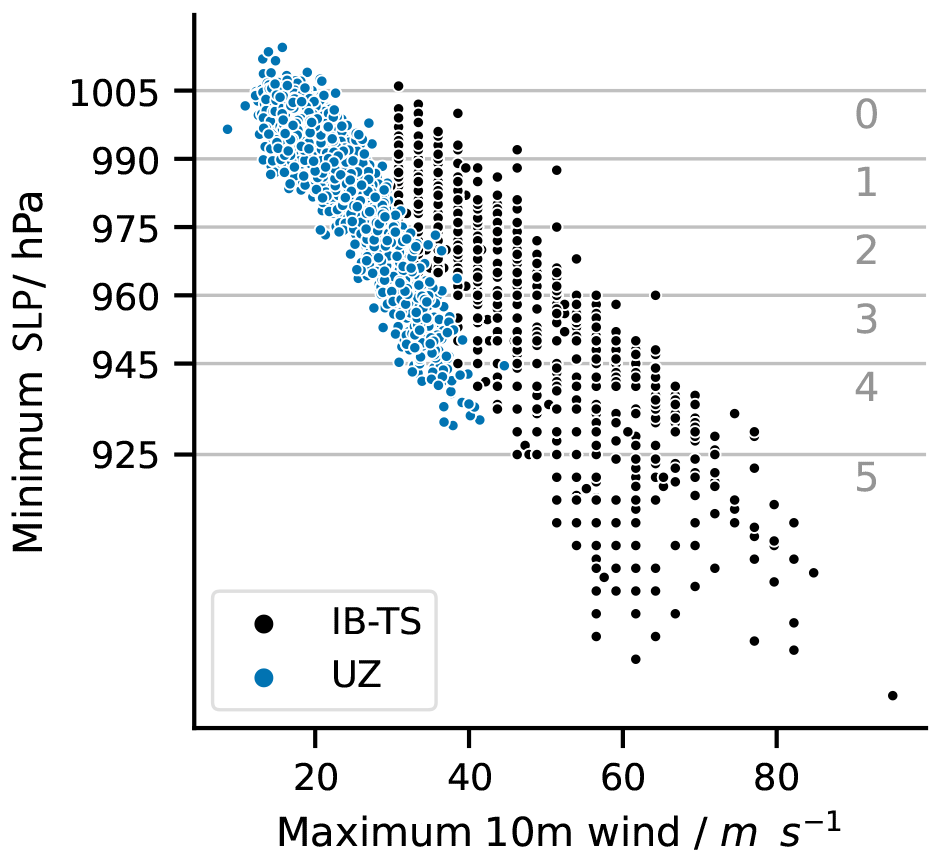
Section 4.2 reported a large and negative bias of ACE for all trackers. This is because the intensity distribution of reanalyzed TCs is different from the intensity distribution of observed TCs (Fig. 10). For all trackers, there is a negative bias for storms of category 2 and larger and an excess of weak storms of categories 0 and −1, which is due to both FAs and hits reanalyzed in ERA5 with a weaker intensity than observed. The two biases compensate so that the overall TC frequencies are comparable in ERA5 and IBTrACS. The difficulty of models in general to simulate strong cyclones is well known (Roberts et al., 2015; Manganello et al., 2012; Strachan et al., 2013; Davis, 2018). It is often illustrated using so-called wind–pressure diagrams such as shown in Fig. 11 for UZ (the wind–pressure diagrams obtained using the other trackers are almost indistinguishable). In agreement with the ACE negative bias and with Fig. 10, Fig. 11 confirms that detected TCs are weaker than observed. They do not follow the same wind–pressure relationship as seen in the observations. In ERA5, the maximum wind speeds of TCs are even more dramatically reduced than the minimum pressure of TCs compared to the observations. The problem is not specific to ERA5. It is encountered in all reanalyses, especially in ERA5's predecessor, ERA-Interim (Hodges et al., 2017; Schenkel and Hart, 2012; Murakami, 2014; Bell et al., 2018). Zarzycki et al. (2021) report an improvement from ERAI to ERA5 in terms of ACE, but it is obvious from Figs. 10 and 11 that ERA5 remains heavily biased.
Figure 10 also reveals that all trackers agree very well for intense TCs of category 2 and above, so the following result holds: all of the detected strong cyclones are detected by all trackers, all of the detected strong cyclones are hits (see the red distributions in the first row of Fig. 1), and there are no FAs among the detected strong cyclones (see the green distributions in the first row of Fig. 1). The spread between trackers is only due to FAs and misses of weak tropical storms.
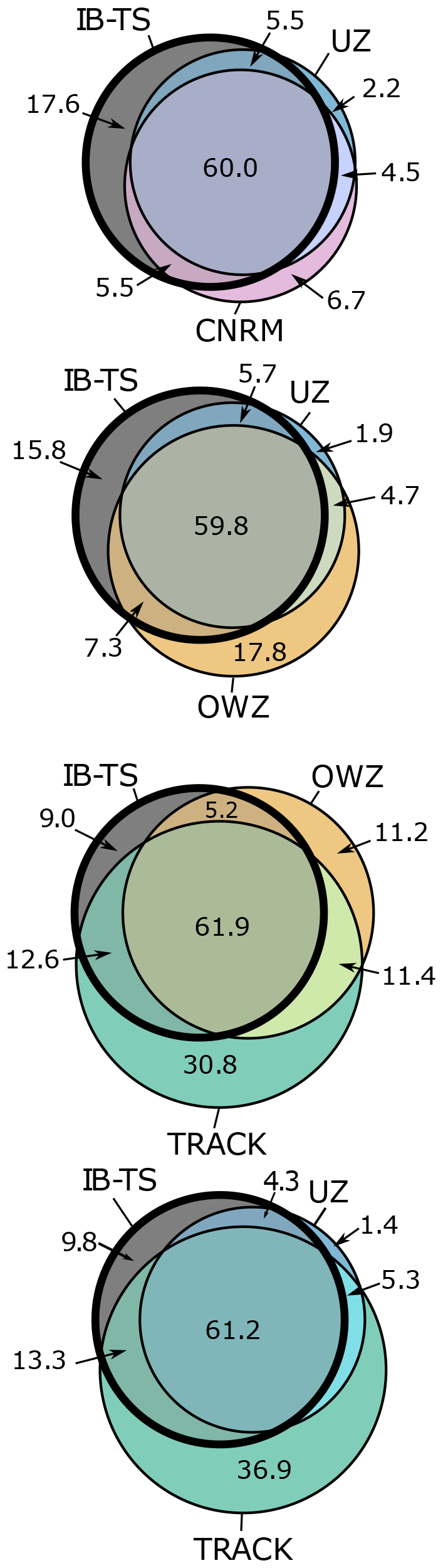
Figure 12Venn diagrams representing common tracks between each algorithm and IB-TS. The figures in the circles are the annual frequency of each group. Venn diagrams are used to show logical relations between sets. Each set of tracks is represented by a circle, whose area is proportional to the size of the set – i.e. the number of tracks. The different circles superpose on an area proportional to the number of tracks that each ensemble have in common. We used the matplotlib-venn package in Python, available on PyPI (https://pypi.org/project/matplotlib-venn/, last access: 22 August 2022) to draw the Venn diagrams.
Now that we better understand what each tracker entails, we can discuss the benefits of using them in isolation or simultaneously.
We found that the use of Venn diagrams, such as shown in Fig. 12, is an interesting method to build a quick and robust intuition about the similarities and differences between the different trackers. They immediately identify the common detections between two algorithms and their respective FAs and misses. First, the most obvious result is that there is a large pool of observed TCs that all trackers detect: there are 3510 tracks in total in IB-TS and about 2400 of them are detected by all trackers, regardless of the Venn diagram considered. This result is simply graphically reflecting the large PODs we found for all trackers. Second, Fig. 12 (first diagram) shows that UZ and CNRM are nearly identical: the number of detections they have in common vastly outnumbers the number of tracks detected by one tracker without being detected by the other. This overlap explains the similar properties noted above for these trackers, both for the globally integrated metrics and properties and for the geographical distributions of detected TCs. We conclude that UZ and CNRM are essentially identical as far as tracking TCs is concerned. Third, these diagrams also nicely illustrate the increasing sensitivity of the different trackers: OWZ is more sensitive than UZ and the CNRM tracker (second diagram) but is itself less sensitive than TRACK (third diagram). Both diagrams also highlight the increasing number of FAs with sensitivity already discussed above.
Below we review the different lines of arguments that could be taken into account for the choice of tracking method. In particular, we keep in mind our objective to apply these trackers to simulation outputs for which we cannot make a pointwise comparison with observations.
It would be tempting to aggregate the four trackers' catalogs. For example, using the union of all trackers would maximize the POD up to 92 %, with the common 8 % of observed storms missed by all trackers corresponding to the weakest and shortest IB-TS storms. However, it would also increase the FAR to 42 %. The opposite approach of using the intersection of all trackers would reduce the FAR down to 6 %, but also cut the POD down to about 65 %. Obviously, none of these simple approaches is ideal by themselves. Similarly, considering the mean value of the metrics might seem attractive: for example, in our case, the mean value of the storms' frequencies features an almost vanishing bias (see Table 3). But as shown by the large associated scatter, this is not significant and only the result of our specific choice of trackers. This approach, though, helps to identify aspects of the detected trajectories that are robust (i.e., tracker-independent). As shown above, this is the case for the negative ACE biases, which result from intrinsic difficulties for TCs to amplify enough in models and reanalyses.
An alternative might be to choose the “best” tracker based on its ability to minimize a given metric or a set of metrics. For example, OWZ minimizes the bias on frequency and TC days (Table 3). This is because, for OWZ, the number of missing TCs is almost equal to the number of FAs. In addition, FAs and missing storms have similar global properties in terms of intensity, latitude of pressure maximum, seasonal cycle, and track durations (compare the red and green distributions in Fig. 1). It means that, on the global scale, FAs can be thought of as a substitute for the misses. This property of OWZ was already noted in ERAI by Bell et al. (2018) and appears to hold here for the particular case of ERA5. However, we caution that this nice global agreement hides a significant regional variability. For OWZ, the number of missing TCs largely outnumbers the number of FAs in the ENP, a bias that is compensated by the larger number of FAs in both the SI and SP oceans (see Fig. 5). These differences point to regional biases, and it is difficult to anticipate how and whether these biases would translate in any numerical simulation.
Another interesting approach is to exploit the respective strengths of the trackers and combine two of them. The fourth Venn diagram in Fig. 12 illustrates such a possibility: the idea is to combine the low FARs of UZ with TRACK's ability to follow the extended life cycles of TCs. Combining UZ and TRACK hits only reduces the POD to 70 % but retains UZ's low FARs. By removing TRACK FAs, which are frequent and close to the Equator, this approach could give stronger support to an analysis of the link between NATL TCs and AEW, such as illustrated in Fig. 9, and still benefit from TRACK's ability to probe the early trajectories of TCs before they are amplified enough to be detected by UZ.
There could be cases for which one is only interested in the strongest tracks. In such cases, the detection skills of all trackers are identical and nearly perfect. As already described above, no detected track beyond category 2 (included) is an FA, and TCs observed with category 4 or 5 are found whatever the tracker. In this case, other properties might become more important, such as the ability to track a larger part of the life cycle provided by OWZ and TRACK.
Another consideration regards the resolution-(in)dependence of the tracking method, or its performance at a given target resolution. Here, the target resolution was that of ERA5, which is about 30 km. The trackers we used either claim to be resolution-independent, or were calibrated at reanalyses with similar resolution, so that the target resolution here is supposedly optimal. It is not guaranteed that any of these trackers will behave similarly at resolutions much lower or much higher than those of ERA5. In particular, trackers embedding a wind threshold might be particularly sensitive to resolution (Walsh et al., 2013). There are also situations for which one would want to assess a set of simulations with a wide range of horizontal resolutions, and for which a resolution-independent method would be preferred. Even though there are arguments in the literature that dynamics-based trackers – e.g., TRACK, OWZ – might be less dependent on resolution than physics-based methodologies (Tory et al., 2013a, b; Raavi and Walsh, 2020), there is no quantitative assessment of this property. In general, we are lacking a quantification of the range of resolutions for which trackers are valid, with or without retuning.
Table 4Comparison of the different trackers' implementations. Computation times are orders of magnitude of the time necessary to sequentially track TCs in one hemisphere over 1 year. They might vary with different machines and setups. (* Kevin Hodges, personal communication, 2022)
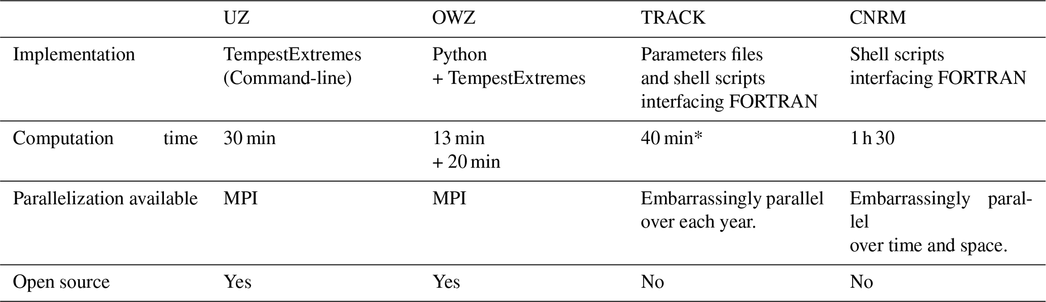
Finally, Table 4 provides practical considerations on the implementation of each tracker. The UZ tracker is implemented using the TempestExtremes command-line software, which is easily parallelizable using MPI, a fully open source. We also benchmarked UZ on 1-hourly data, proving that the computation time scales linearly with temporal resolution. The OWZ necessitates two steps: the first is the computation of the OWZ variable, which is done in Python, and the second is the tracking itself, done here with TempestExtremes (and therefore parallelized using MPI as well). The code for OWZ is provided along with this paper. TRACK is run using shell scripts that read input from text files and run the FORTRAN code. Since it performs spectral filtering, it needs to be run globally, and because of the stitching step that is not independent, it is tricky to split it in the middle of a TC season. Therefore, the embarrassingly parallel potential is limited to parallelizing over the years. TRACK code is not open source but available upon request. The CNRM tracker is also implemented in FORTRAN, interfaced with shell scripts. It does not have any parallelization implemented so far, but it can be used embarrassingly parallel over space or time. In terms of computation time, if no parallelization is used, UZ, OWZ, and TRACK are roughly equivalent, while CNRM requires about twice as much time. The best potential for parallel acceleration is presented by UZ, followed by OWZ, although with a slightly reduced potential because the TempestExtremes part corresponds to two-thirds of its processing.
In the present paper we have applied four tracking algorithms to ERA5 over the period 1980–2019. These trackers are UZ (Zarzycki and Ullrich, 2017; Ullrich et al., 2021), OWZ (Tory et al., 2013b; Bell et al., 2018), TRACK (Hodges, 1994) and the CNRM tracker (Chauvin et al., 2006). The PODs evaluated against IBTrACS range from 75 % to 85 %, and the FARs vary between 19 % and 60 %. Tracks missed by the trackers mostly correspond to weak tropical storms. One possibility is that missing tracks correspond to storms that were not reanalyzed with sufficient intensity in ERA5. The false alarms correspond to either weak tropical disturbances or extra-tropical cyclones. We derived two objective filtering methods to target these extra-tropical false alarms. The first one is based on the environment of the tracks, i.e., it relies on the relative positions of the detected tracks and the upper troposphere sub-tropical jet (STJ). The second one is based on the third Hart phase space parameter, the upper-level thermal wind (VTU), i.e., it allows us to determine whether the core of the storm is warm or cold. Both post-treatments can be applied identically to any catalog of TC tracks. For the four trackers we used for this study, we found a dramatic reduction of FAs for all trackers except OWZ: FARs range from 9 to 36 % after post-treatment, which correspond to reductions of up to 76 %.
We then studied how several traditional metric biases depend on the choice of the tracker. The TC frequencies are highly sensitive to the algorithm. This is consistent with the study of Horn et al. (2014), who found that the intensity threshold drives the difference of TC frequencies found using several physics-based trackers. Our analysis shows that this is true when including dynamics-based trackers as well. The number of TC days also varies with the algorithm, i.e., tracks' mean duration is smaller than the observation for UZ and CNRM, similar for OWZ, and longer for TRACK. Both metrics' sensitivity reflects the large variability in trackers' selectivity regarding weak storms. They are also consistent with Raavi and Walsh (2020), who found that the CSIRO tracker features simultaneously lower TC frequencies and shorter tracks than OWZ. However, other metrics do not suffer from that variability. The ACE is almost uniform across trackers because it is mostly sensitive to the strongest TCs, for which all trackers agree.
It should be noted that these global scores are heavily weighted by the most active oceanic basin, namely the WNP ocean. The TC frequencies in that particular basin compare well with the observations and the scatter across trackers remains moderate (Fig. 6). This is more of an exception rather than the rule. In the SI and SP oceans, TRACK bias in TC frequency is positive and large, while the other trackers are close to IB-TS. In the ENP, TRACK bias in TC frequency is small, while the other trackers' biases are negative and large. The NATL ocean is peculiar because all trackers feature negative biases. Contrasted results are also found for the number of TC days. They are not easy to understand. They may result from inhomogeneities in IBTrACS due to differences in reporting methods by each agency and/or from inhomogeneities in ERA5 because of the varying amount and density ofthe observations available for assimilation. Moreover, TCs may have different intrinsic properties in the different oceanic basins. It will be interesting to investigate whether these geographical differences hold in model results in order to disentangle these alternatives.
Finally, it is important to keep in mind that deriving detection scores implicitly implies that some sort of Boolean-reality threshold exists between what is a TC or not. Of course, this is not the case in reality where these meteorological systems form a continuum. Hence, any attempt to categorize them is intrinsically somewhat arbitrary. In the same way that classification based on satellite imagery or fixed wind thresholds is, to some extent, subjective, trackers' thresholds are arbitrary and artificially create a strict limit in the gray zone that separates tropical disturbances, storms, and cyclones. One should not forget that these limits are trackers' design choices that reflect the goals of their designers. OWZ was created to study precursors and to be resolution-independent (Tory et al., 2013b). TRACK aims to detect all vorticity perturbations, while TC identification is secondary (Hodges, 1994). The UZ and the CNRM trackers were calibrated using a series of observed metrics in the reanalyses (Zarzycki and Ullrich, 2017). These design choices are reflected in past and present results and will affect future analyses of both reanalyses and models.
| TC | tropical cyclone |
| TS | tropical storm |
| SLP | sea-level pressure |
| SSHS | Saffir–Simpson Hurricane Scale |
| NH | Northern Hemisphere |
| SH | Southern Hemisphere |
| IBTrACS | International Best Track Archive for |
| Climate Stewardship | |
| IB-TS | Tropical storm subset of IBTrACS |
| IB-TC | Tropical cyclone subset of IBTrACS |
| ERA5 | Fifth European ReAnalysis |
| UZ | Ullrich & Zarzycki |
| OWZ | Obuko-Weiss-Zeta |
| CNRM | Centre National de Recherches |
| Météorologiques | |
| FA | false alarm |
| FAR | false alarm rate |
| POD | probability of detection |
| ETC | extra-tropical cyclone |
| NATL | North Atlantic |
| WNP | western North Pacific |
| ENP | eastern North Pacific |
| SP | South Pacific |
| NI | North Indian |
| SI | South Indian |
| ACE | accumulated cyclonic energy |
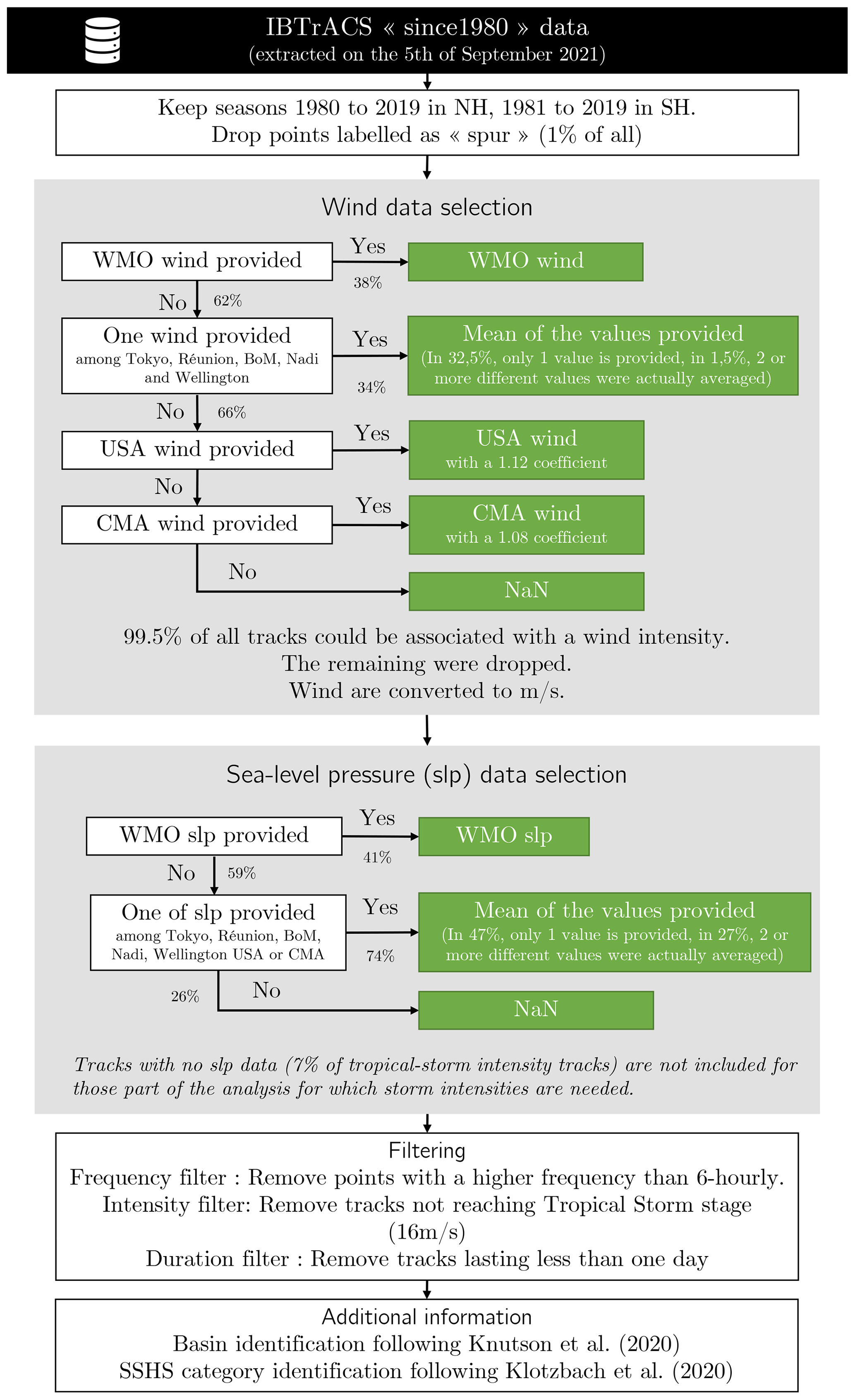
Figure B1Workflow chart describing the treatment of the IBTrACS database in out study. The 1.08 coefficient to convert 3-min sustained winds to 10-min sustained winds was obtained using a linear regression on the data for which we had both.
Table B1Synthesis of the trackers' criteria. All subscripts except 10 correspond to pressure levels in hPa.
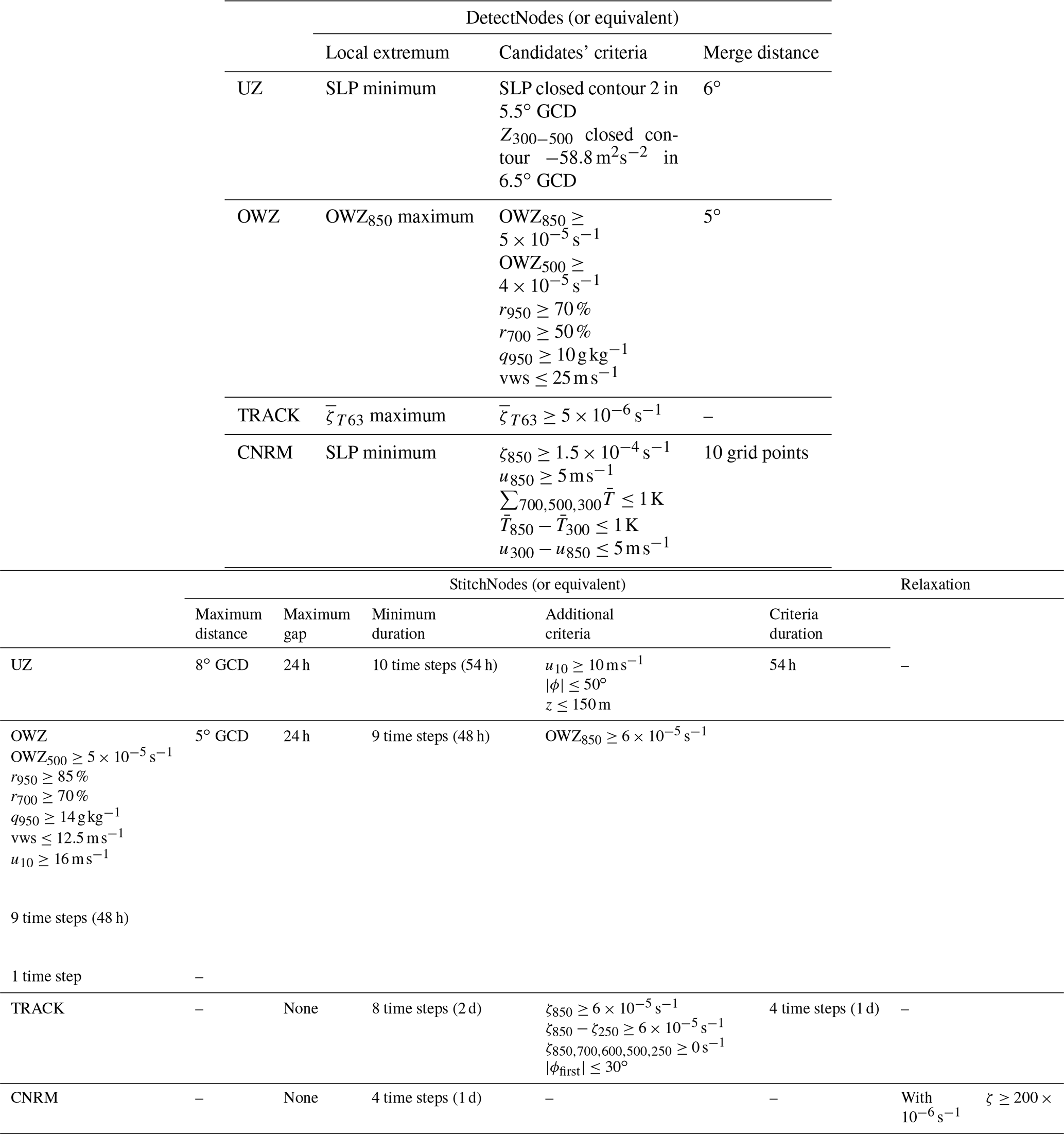
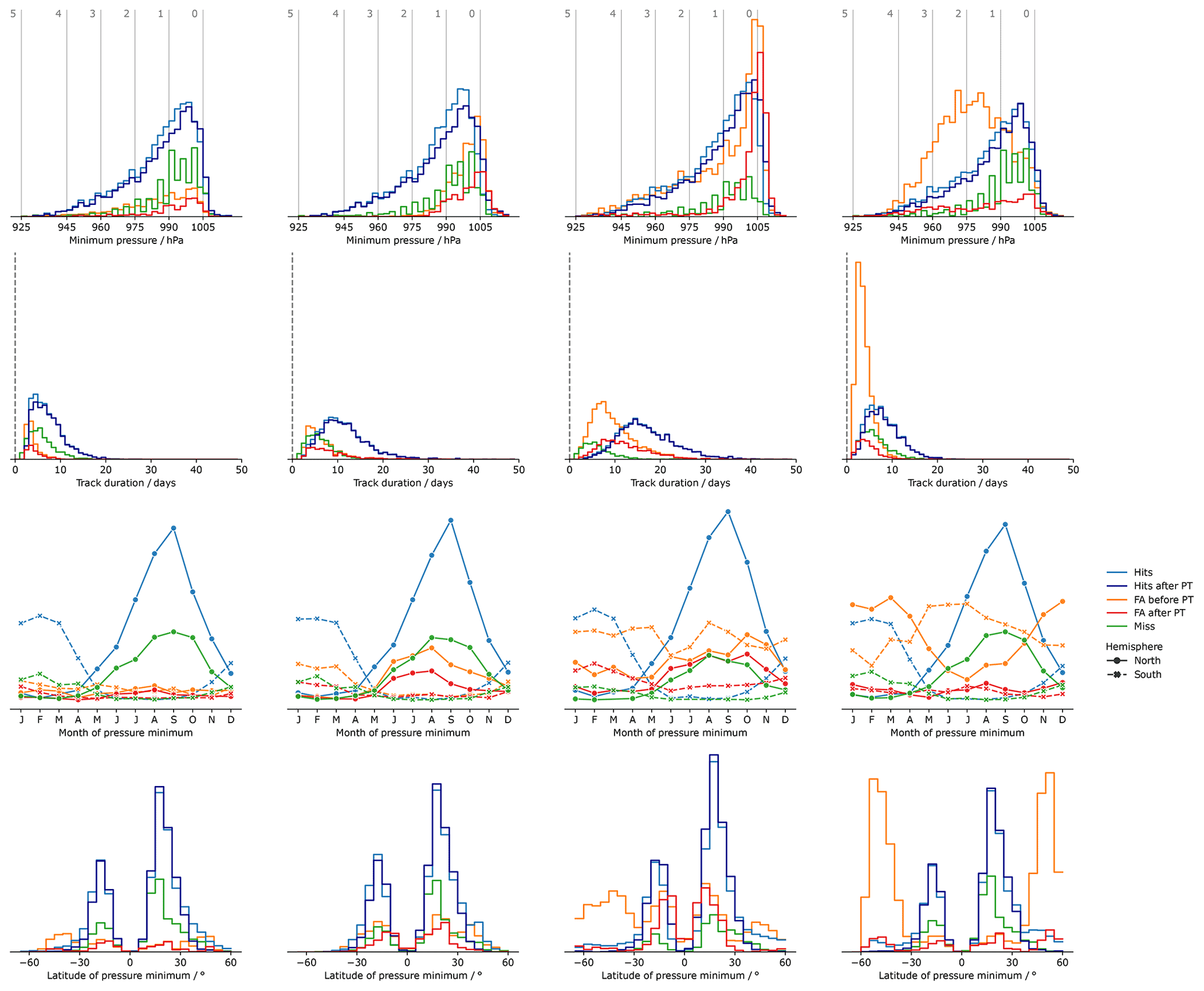
Figure B2Same figure as Fig. 1, but for the VTU post-treatment: characterization of the FAs of each algorithm. The first line of distributions correspond to the minimum SLP, the second line to the latitude of the pressure minimum, and the third line to the track duration. In all plots, blue distribution correspond to the hits, orange to the FAs before the VTU post-treatment, and red to the FAs remaining after the VTU post-treatment.
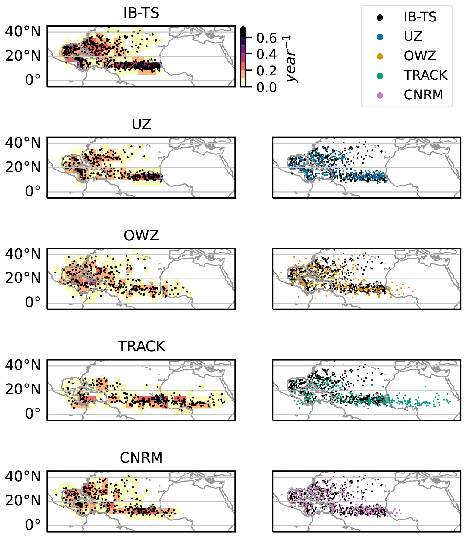
Figure B3Extension of Fig. 9 for all four trackers. First observed/detected points in IB-TS, TRACK, and UZ. The left column shows the first points along with the corresponding density. The right column overlays IB-TS track's first point with ERA5 track's first point as detected tracks by each tracker.
C1 UZ
The code for UZ is exactly the same as in Ullrich et al. (2021), we only adapted it to our own data infrastructure.
C2 OWZ
For this study, we adapted the OWZ algorithm presented in Sect. 2.3 to be used in the TempestExtremes framework (Ullrich and Zarzycki, 2017; Ullrich et al., 2021). Doing so involved a change in part of the methodology, and the arbitrary choice of some criteria that are required by the TempestExtremes framework.
C2.1 Original algorithm
In Bell et al. (2018), the OWZ algorithm applied on ERA-Interim data is described as follows:
-
Each grid point at each time step is assessed based on the initial threshold values.
-
Clusters (or “clumps” in Tory et al., 2013b) are formed by gathering neighboring points that satisfy the initial thresholds and that are supposed to represent a single circulation at that point in time.
-
Circulations from step (2) are linked through time by estimating their position in relation to the circulation's expected position based on an averaged 4∘ × 4∘ steering wind at 700 hPa.
-
Tracks are terminated when no circulation match is found in the next 2 time steps within a latitude-dependent radius (∼350 km).
-
Tracks are declared TC if the core thresholds are satisfied for five consecutive 12 h periods.
The thresholds are provided in their Table 1.
Tory et al. (2013b) further specifies that “clumps in close proximity are reduced to one clump by discarding the weaker or smaller clumps”, and that each clump must satisfy a set of clump conditions: “a minimum size limit, and a land-impact condition”. The minimum size limit is two grid points and the radius to look for weaker or smaller clumps is 550 km. The land-impact condition tests whether the point is over the land or the ocean. In this paper, the latitude-dependent radius of step (4) “varies linearly from 600 to 400 km between 15 and 30∘ latitude in both hemispheres, with constant values outside this latitude band”, which does not correspond with the 350 km specified by Bell et al. (2018).
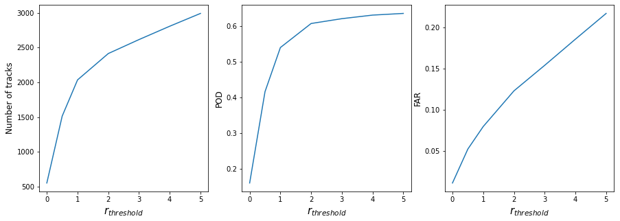
Figure C1Sensitivity of the number of tracks, the POD, and the FAR of OWZ for different values of rthreshold.
C2.2 TempestExtremes Adaptation
The TempestExtremes nodal feature detection framework (DetectNodes + StitchNodes) does not work with the same paradigm, but still allows us to implement a very similar algorithm. The fundamental principle in DetectNodes is to track a local extremum of one variable. It can then merge all extrema in a given radius (rmerge) into the largest one, and the position of the extremum is considered the center of the detected feature. One can also add discriminatory criteria, either (i) in terms of thresholds to be satisfied for given variables at the grid point of the extremum, or by one grid point in a given radius rthreshold from the center, or (ii) in terms of a closed contour. (see Ullrich and Zarzycki, 2017). The subsequent StitchNodes uses a nearest-neighbors approach to link consecutive points within a maximum distance rrange. In this command, one can also allow for a gap to exist in the track, and check additional thresholds that must be satisfied for a given number of points in order to validate the track.
Here we choose to look for a local maximum of OWZ, and to merge all weaker maxima in a 5∘ GCD (≈550 km in the original algorithm). Thresholds from the original algorithm must be satisfied by at least one grid point in a rthreshold radius (that will be determined from the following sensitivity tests). In the StitchNodes command, we look for consecutive points within a rrange radius (that will also be determined from the following sensitivity tests). A 24 h gap is allowed, corresponding to the “next 12 h time steps”). In addition to this, core thresholds are assessed within the same rthreshold radius, and must be satisfied for at least nine 6-hourly time steps. Core thresholds include the “land-impact condition” that we implement using the land–ocean mask and consider as ocean points with less than 50 % of land. The minimum duration is set to 48 h, corresponding to the 9 6-hourly time steps, so that it is not a discriminatory criterion but helps to accelerate the computation.
At this stage, we have two parameters left to determine: rthreshold and rrange, for which we conduct independent sensitivity tests.
C2.3 Sensitivity analysis
In the original algorithm, the thresholds must all be satisfied in the same grid point. However, it was used on ERA-Interim data interpolated onto a 1∘ × 1∘ grid, whereas ERA5 data present itself with 0.25∘ × 0.25∘ grid points. One can expect that this higher resolution might allow for the formation of an eye in the circulation, so that all the thresholds might be verified in the wall rather than in the center of the circulation. We test seven values for rthreshold: 0∘ (thresholds must be passed at the center), 0.5, 1∘.
The 350 km range in Bell et al. (2018) corresponds to 3∘, whereas the [400, 600 km] range in Tory et al. (2013b) correspond to [3.5, 5.5∘]. In UZ, the range is set to 8∘. We test rrange values between 3 and 8∘.
To assess the sensitivity of the detection to these thresholds, we compute the number of tracks detected. We also pair detected tracks with observed IB-TS tracks following the procedure described in Sect. 2.4, and compute the FAR and the probability of detection.
The sensitivity to the rrange parameter is low (not shown), in accordance with results in UZ by Zarzycki and Ullrich (2017). We choose rrange=5∘ in the middle of Tory et al. (2013b) range. Figure C1 shows the sensitivity of the three metrics to the rthreshold parameter. We can see that for rthreshold≥2, the POD saturate and all additional tracks are false positive. For this reason, we keep rthreshold=2.
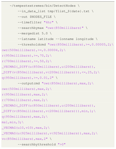
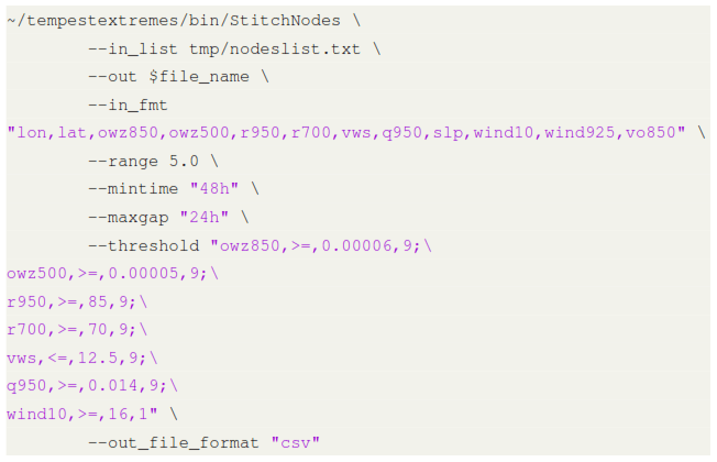
Here we validate our matching method through a few sanity checks. They show that the pairing methodology is not very sensitive.
Figure D1 shows the distribution of the numbers of overlapping time steps, i.e., the time for which two paired tracks are closer than 300 km. By construction of our method, there must be at least one of them. It is compared to the distribution of lifetime in IB-TS. Figure D2 shows the proportion of the observed lifetime matching the corresponding ERA5 track, when it exists. Figure D3 shows the distribution of the distance between the observed and detected tracks, averaged over the overlapping time steps for each pair of tracks. Each distribution is provided for each tracker as a boxplot that indicates the 1st, 25th, 50th, 75th, and 99th percentiles.
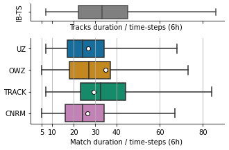
Figure D1Distribution of the duration of the overlap between matching detected and observed tracks. Whiskers display the 1st and 99th percentiles, and white points show the mean of the distributions. Outliers are not shown.

Figure D2Distribution of the duration of the overlap between matching detected and observed tracks. Whiskers display the 1st and 99th percentiles, and white points show the mean of the distributions. Outliers are not shown.
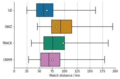
Figure D3Distribution of distance between matching detected and observed tracks. Whiskers display the 1st and 99th percentiles, and white points show the mean of the distributions. Outliers are not shown.
Figure D1 shows that despite the fact that our methodology imposes only one overlapping point, more than 99 % of the pairs, whatever the tracker, match for at least 5 time steps. It shows that the matching is not sensitive to this threshold. In fact, Fig. D3 shows that in most cases, observed tracks are matched for more than half of the observed lifetime (Fig. D3). This proportion relates to the mean-detected lifetime by each tracker displayed in Fig. 7. Moreover, the matching distance is of the order of a few grid cells, inferior or close to 100 km regardless of the trackers, with a slightly better accuracy of the trackers that use SLP as their center. All this gives us confidence in the fact that the tracks that are paired together are indeed corresponding, because they are close to one another for a significant part of their lifetime.
Figure D3 (TRACK line) can be compared to Hodges et al. (2017), who found that the TRACK match distance was about 1∘ for other reanalyses tracked with TRACK. The improvement can be related to the increase in resolution.
ERA5 data are available on the Copernicus Climate Change Service Climate Data Store (CDS, https://cds.climate.copernicus.eu/cdsapp#!/dataset/reanalysis-era5-pressure-levels, last access: 22 August 2022). The IBTrACS database is provided by NOAA at https://www.ncdc.noaa.gov/ibtracs/ (last access: 22 August 2022).
All the scripts used to produce the present paper's results are available at https://doi.org/10.5281/zenodo.6424432 (Bourdin, 2022a). These include the code to run the UZ and OWZ trackers and the original TRACK and CNRM databases, the code for the post-treatment and the tracks matching Python scripts for the whole analysis, the code to reproduce the figures, and finally, a copy of v.0.5 of the dynamicoPy package used in the Python scripts (https://doi.org/10.5281/zenodo.7015245; Bourdin, 2022b).
SB designed and carried out the study under the supervision of SF. All authors provided critical feedback and helped to shape the whole study. WD ran the CNRM tracker under the supervision of JC and FC. SB and SF prepared the manuscript, with input from all co-authors. SB did the figures. SF obtained the funding.
The contact author has declared that none of the authors has any competing interests.
Publisher's note: Copernicus Publications remains neutral with regard to jurisdictional claims in published maps and institutional affiliations.
The research is supported by public funding to the CEA and CNRM. Stella Bourdin and Sébastien Fromang were also financially supported by the EUR IPSL-Climate Graduate School through the ICOCYCLONES project.
The authors are grateful to Kevin Hodges for providing the TRACK dataset, for insightful scholar discussion and literature provision and for his review of an earlier version of this manuscript. The authors thank Paul Ullrich and Colin Zarzycki for their help regarding TempestExtremes. Stella Bourdin thanks colleagues at the LSCE for helpful discussion and feedback, and especially Robin Noyelle for the idea of using the Hart phase space. The authors appreciated the constructive and insightful comments from Malcolm Roberts and one anonymous reviewer, which helped improve the present manuscript.
This research has been supported by the Centre National de la Recherche Scientifique (LEFE/CYPRESSA) and the Sorbonne Université (EUR IPSL-Climate Graduate School).
This paper was edited by Travis O'Brien and reviewed by Malcolm Roberts and one anonymous referee.
Arias, P., Bellouin, N., Coppola, E., Jones, R., Krinner, G., Marotzke, J., Naik, V., Palmer, M., Plattner, G.-K., Rogelj, J., Rojas, M., Sillmann, J., Storelvmo, T., Thorne, P., Trewin, B., Achuta Rao, K., Adhikary, B., Allan, R., Armour, K., Bala, G., Barimalala, R., Berger, S., Canadell, J., Cassou, C., Cherchi, A., Collins, W., Collins, W., Connors, S., Corti, S., Cruz, F., Dentener, F., Dereczynski, C., Di Luca, A., Diongue Niang, A., Doblas-Reyes, F., Dosio, A., Douville, H., Engelbrecht, F., Eyring, V., Fischer, E., Forster, P., Fox-Kemper, B., Fuglestvedt, J., Fyfe, J., Gillett, N., Goldfarb, L., Gorodetskaya, I., Gutierrez, J., Hamdi, R., Hawkins, E., Hewitt, H., Hope, P., Islam, A., Jones, C., Kaufman, D., Kopp, R., Kosaka, Y., Kossin, J., Krakovska, S., Lee, J.-Y., Li, J., Mauritsen, T., Maycock, T., Meinshausen, M., Min, S.-K., Monteiro, P., Ngo-Duc, T., Otto, F., Pinto, I., Pirani, A., Raghavan, K., Ranasinghe, R., Ruane, A., Ruiz, L., Sallée, J.-B., Samset, B., Sathyendranath, S., Seneviratne, S., Sörensson, A., Szopa, S., Takayabu, I., Tréguier, A.-M., van den Hurk, B., Vautard, R., von Schuckmann, K., Zaehle, S., Zhang, X., and Zickfeld, K.: Technical Summary, 33–144, Cambridge University Press, Cambridge, United Kingdom and New York, NY, USA, https://www.ipcc.ch/report/ar6/wg1/downloads/report/IPCC_AR6_WGI_TS.pdf (last access: 22 August 2022), 2021. a
Avila, L. A., Pasch, R. J., and Jiing, J.-G.: Atlantic tropical systems of 1996 and 1997: Years of contrasts, Mon. Weather Rev., 128, 3695–3706, 2000. a
Ayrault, F.: Environnement, structure et évolution des dépressions météorologiques: réalité climatologique et modèles types, PhD thesis, Toulouse, 3, 1998. a
Bell, S. S., Chand, S. S., Tory, K. J., and Turville, C.: Statistical Assessment of the OWZ Tropical Cyclone Tracking Scheme in ERA-Interim, J. Climate, 31, 2217–2232, https://doi.org/10.1175/JCLI-D-17-0548.1, 2018. a, b, c, d, e, f, g, h, i, j, k, l
Bengtsson, L., Hodges, K. I., Esch, M., Keenlyside, N., Kornblueh, L., Luo, J.-J., and Yamagata, T.: How may tropical cyclones change in a warmer climate?, Tellus A, 59, 539–561, https://doi.org/10.1111/j.1600-0870.2007.00251.x, 2007. a
Bourdin, S.: Bourdin et al. 2022, Intercomparison of Four Tropical Cyclones Detection Algorithms on ERA5 – Code and Data (Version v1), Zenodo [code and data], https://doi.org/10.5281/zenodo.6424432, 2022a. a
Bourdin, S.: DynamicoPy v0.6 (0.6), Zenodo [code and data], https://doi.org/10.5281/zenodo.7015245, 2022b. a
Camargo, S. J.: Global and Regional Aspects of Tropical Cyclone Activity in the CMIP5 Models, J. Climate, 26, 9880–9902, https://doi.org/10.1175/JCLI-D-12-00549.1, 2013. a
Camargo, S. J. and Wing, A. A.: Tropical cyclones in climate models, WIREs Climate Change, 7, 211–237, https://doi.org/10.1002/wcc.373, 2016. a
Camargo, S. J. and Zebiak, S. E.: Improving the Detection and Tracking of Tropical Cyclones in Atmospheric General Circulation Models, Weather Forecast., 17, 1152–1162, https://doi.org/10.1175/1520-0434(2002)017<1152:ITDATO>2.0.CO;2, 2002. a, b
Cattiaux, J., Chauvin, F., Bousquet, O., Malardel, S., and Tsai, C.-L.: Projected Changes in the Southern Indian Ocean Cyclone Activity Assessed from High-Resolution Experiments and CMIP5 Models, J. Climate, 33, 4975–4991, https://doi.org/10.1175/JCLI-D-19-0591.1, 2020. a
Chauvin, F., Royer, J.-F., and Déqué, M.: Response of hurricane-type vortices to global warming as simulated by ARPEGE-Climat at high resolution, Clim. Dynam., 27, 377–399, https://doi.org/10.1007/s00382-006-0135-7, 2006. a, b, c, d
Chauvin, F., Pilon, R., Palany, P., and Belmadani, A.: Future changes in Atlantic hurricanes with the rotated-stretched ARPEGE-Climat at very high resolution, Clim. Dynam., 54, 947–972, https://doi.org/10.1007/s00382-019-05040-4, 2020. a
Chavas, D. R., Reed, K. A., and Knaff, J. A.: Physical understanding of the tropical cyclone wind-pressure relationship, Nat. Commun., 8, 1360, https://doi.org/10.1038/s41467-017-01546-9, 2017. a
Davis, C. A.: Resolving Tropical Cyclone Intensity in Models, Geophys. Res. Lett., 45, 2082–2087, https://doi.org/10.1002/2017GL076966, 2018. a
Duvel, J.-P.: On vortices initiated over West Africa and their impact on North Atlantic tropical cyclones, Mon. Weather Re., 149, 585–601, 2021. a
Haarsma, R. J., Roberts, M. J., Vidale, P. L., Senior, C. A., Bellucci, A., Bao, Q., Chang, P., Corti, S., Fučkar, N. S., Guemas, V., von Hardenberg, J., Hazeleger, W., Kodama, C., Koenigk, T., Leung, L. R., Lu, J., Luo, J.-J., Mao, J., Mizielinski, M. S., Mizuta, R., Nobre, P., Satoh, M., Scoccimarro, E., Semmler, T., Small, J., and von Storch, J.-S.: High Resolution Model Intercomparison Project (HighResMIP v1.0) for CMIP6, Geosci. Model Dev., 9, 4185–4208, https://doi.org/10.5194/gmd-9-4185-2016, 2016. a
Harper, B., Kepert, J. D., and Ginger, J. D.: Guidelines for converting between various wind averaging periods in tropical cyclone conditions, world Meteorological Organization Rep., 54 pp., http://citeseerx.ist.psu.edu/viewdoc/download?doi=10.1.1.730.9719&rep=rep1&type=pdf (last access: 22 August 2022), 2010. a
Hart, R. E.: A Cyclone Phase Space Derived from Thermal Wind and Thermal Asymmetry, Mon. Weather Rev., 131, 585–616, https://doi.org/10.1175/1520-0493(2003)131<0585:ACPSDF>2.0.CO;2, 2003. a, b, c
Hersbach, H., Bell, B., Berrisford, P., Hirahara, S., Horányi, A., Muñoz-Sabater, J., Nicolas, J., Peubey, C., Radu, R., Schepers, D., Simmons, A., Soci, C., Abdalla, S., Abellan, X., Balsamo, G., Bechtold, P., Biavati, G., Bidlot, J., Bonavita, M., De Chiara, G., Dahlgren, P., Dee, D., Diamantakis, M., Dragani, R., Flemming, J., Forbes, R., Fuentes, M., Geer, A., Haimberger, L., Healy, S., Hogan, R. J., Hólm, E., Janisková, M., Keeley, S., Laloyaux, P., Lopez, P., Lupu, C., Radnoti, G., de Rosnay, P., Rozum, I., Vamborg, F., Villaume, S., and Thépaut, J.-N.: The ERA5 global reanalysis, Q. J. Roy. Meteor. Soc., 146, 1999–2049, https://doi.org/10.1002/qj.3803, 2020. a, b, c
Hodges, K., Cobb, A., and Vidale, P. L.: How Well Are Tropical Cyclones Represented in Reanalysis Datasets?, J. Climate, 30, 5243–5264, https://doi.org/10.1175/JCLI-D-16-0557.1, 2017. a, b, c, d, e, f, g, h, i, j, k, l, m
Hodges, K. I.: A General Method for Tracking Analysis and Its Application to Meteorological Data, Mon. Weather Rev., 122, 2573–2586, https://doi.org/10.1175/1520-0493(1994)122<2573:AGMFTA>2.0.CO;2, 1994. a, b, c, d
Hodges, K. I.: Feature Tracking on the Unit Sphere, Mon. Weather Rev., 123, 3458–3465, https://doi.org/10.1175/1520-0493(1995)123<3458:FTOTUS>2.0.CO;2, 1995. a
Hodges, K. I.: Adaptive Constraints for Feature Tracking, Mon. Weather Rev., 127, 1362–1373, https://doi.org/10.1175/1520-0493(1999)127<1362:ACFFT>2.0.CO;2, 1999. a
Hopsch, S. B., Thorncroft, C. D., Hodges, K., and Aiyyer, A.: West African storm tracks and their relationship to Atlantic tropical cyclones, J. Climate, 20, 2468–2483, 2007. a
Horn, M., Walsh, K., Zhao, M., Camargo, S. J., Scoccimarro, E., Murakami, H., Wang, H., Ballinger, A., Kumar, A., Shaevitz, D. A., Jonas, J. A., and Oouchi, K.: Tracking Scheme Dependence of Simulated Tropical Cyclone Response to Idealized Climate Simulations, J. Climate, 27, 9197–9213, https://doi.org/10.1175/JCLI-D-14-00200.1, 2014. a, b, c
Klotzbach, P. J., Bell, M. M., Bowen, S. G., Gibney, E. J., Knapp, K. R., and Schreck, C. J.: Surface Pressure a More Skillful Predictor of Normalized Hurricane Damage than Maximum Sustained Wind, B. Am. Meteorol. Soc., 101, E830–E846, https://doi.org/10.1175/BAMS-D-19-0062.1, 2020. a, b, c, d
Knapp, K. R., Kruk, M. C., Levinson, D. H., Diamond, H. J., and Neumann, C. J.: The International Best Track Archive for Climate Stewardship (IBTrACS): Unifying Tropical Cyclone Data, B. Am. Meteorol. Soc., 91, 363–376, https://doi.org/10.1175/2009BAMS2755.1, 2010. a, b, c, d, e
Knapp, K. R., Diamond, H. J., Kossin, J. P., Kruk, M. C., and Schreck, C.: International best track archive for climate stewardship (IBTrACS) project, version 4, https://doi.org/10.25921/82ty-9e16, subset: since1980, 2018. a
Knutson, T., Camargo, S. J., Chan, J. C. L., Emanuel, K., Ho, C.-H., Kossin, J., Mohapatra, M., Satoh, M., Sugi, M., Walsh, K., and Wu, L.: Tropical Cyclones and Climate Change Assessment: Part I: Detection and Attribution, B. Am. Meteorol. Soc., 100, 1987–2007, https://doi.org/10.1175/BAMS-D-18-0189.1, 2019. a
Knutson, T., Camargo, S. J., Chan, J. C. L., Emanuel, K., Ho, C.-H., Kossin, J., Mohapatra, M., Satoh, M., Sugi, M., Walsh, K., and Wu, L.: Tropical Cyclones and Climate Change Assessment: Part II: Projected Response to Anthropogenic Warming, B. Am. Meteorol. Soc., 101, E303–E322, https://doi.org/10.1175/BAMS-D-18-0194.1, 2020. a, b
Knutson, T. R., Sirutis, J. J., Zhao, M., Tuleya, R. E., Bender, M., Vecchi, G. A., Villarini, G., and Chavas, D.: Global Projections of Intense Tropical Cyclone Activity for the Late Twenty-First Century from Dynamical Downscaling of CMIP5/RCP4.5 Scenarios, J. Climate, 28, 7203–7224, https://doi.org/10.1175/JCLI-D-15-0129.1, 2015. a
Landsea, C. W.: A climatology of intense (or major) Atlantic hurricanes, Mon. Weather Rev., 121, 1703–1713, 1993. a
Manganello, J. V., Hodges, K. I., Kinter, J. L., Cash, B. A., Marx, L., Jung, T., Achuthavarier, D., Adams, J. M., Altshuler, E. L., Huang, B., Jin, E. K., Stan, C., Towers, P., and Wedi, N.: Tropical Cyclone Climatology in a 10-km Global Atmospheric GCM: Toward Weather-Resolving Climate Modeling, J. Climate, 25, 3867–3893, https://doi.org/10.1175/JCLI-D-11-00346.1, 2012. a, b
Murakami, H.: Tropical cyclones in reanalysis data sets, Geophysical Research Letters, 41, 2133–2141, https://doi.org/10.1002/2014GL059519, 2014. a, b, c, d
Murakami, H., Vecchi, G. A., Underwood, S., Delworth, T. L., Wittenberg, A. T., Anderson, W. G., Chen, J.-H., Gudgel, R. G., Harris, L. M., Lin, S.-J., and Zeng, F.: Simulation and Prediction of Category 4 and 5 Hurricanes in the High-Resolution GFDL HiFLOR Coupled Climate Model, J. Climate, 28, 9058–9079, https://doi.org/10.1175/JCLI-D-15-0216.1, 2015. a
Patricola, C. M., Saravanan, R., and Chang, P.: The response of Atlantic tropical cyclones to suppression of African easterly waves, Geophys. Res. Lett., 45, 471–479, 2018. a
Raavi, P. H. and Walsh, K. J. E.: Sensitivity of Tropical Cyclone Formation to Resolution-Dependent and Independent Tracking Schemes in High-Resolution Climate Model Simulations, Earth Space Sci., 7, e2019EA000906, https://doi.org/10.1029/2019EA000906, 2020. a, b, c
Roberts, M. J., Vidale, P. L., Mizielinski, M. S., Demory, M.-E., Schiemann, R., Strachan, J., Hodges, K., Bell, R., and Camp, J.: Tropical Cyclones in the UPSCALE Ensemble of High-Resolution Global Climate Models, J. Climate, 28, 574–596, https://doi.org/10.1175/JCLI-D-14-00131.1, 2015. a
Roberts, M. J., Camp, J., Seddon, J., Vidale, P. L., Hodges, K., Vanniere, B., Mecking, J., Haarsma, R., Bellucci, A., Scoccimarro, E., Caron, L.-P., Chauvin, F., Terray, L., Valcke, S., Moine, M.-P., Putrasahan, D., Roberts, C., Senan, R., Zarzycki, C., and Ullrich, P.: Impact of Model Resolution on Tropical Cyclone Simulation Using the HighResMIP–PRIMAVERA Multimodel Ensemble, J. Climate, 33, 2557–2583, https://doi.org/10.1175/JCLI-D-19-0639.1, 2020a. a, b, c, d, e, f, g, h
Roberts, M. J., Camp, J., Seddon, J., Vidale, P. L., Hodges, K., Vannière, B., Mecking, J., Haarsma, R., Bellucci, A., Scoccimarro, E., Caron, L.-P., Chauvin, F., Terray, L., Valcke, S., Moine, M.-P., Putrasahan, D., Roberts, C. D., Senan, R., Zarzycki, C., Ullrich, P., Yamada, Y., Mizuta, R., Kodama, C., Fu, D., Zhang, Q., Danabasoglu, G., Rosenbloom, N., Wang, H., and Wu, L.: Projected Future Changes in Tropical Cyclones Using the CMIP6 HighResMIP Multimodel Ensemble, Geophys. Res. Lett., 47, e2020GL088662, https://doi.org/10.1029/2020GL088662, 2020b. a, b
Schenkel, B. A. and Hart, R. E.: An Examination of Tropical Cyclone Position, Intensity, and Intensity Life Cycle within Atmospheric Reanalysis Datasets, J. Climate, 25, 3453–3475, https://doi.org/10.1175/2011JCLI4208.1, 2012. a, b
Simpson, R. H. and Saffir, H.: The hurricane disaster potential scale, Weatherwise, 27, 169, 1974. a
Strachan, J., Vidale, P. L., Hodges, K., Roberts, M., and Demory, M.-E.: Investigating Global Tropical Cyclone Activity with a Hierarchy of AGCMs: The Role of Model Resolution, J. Climate, 26, 133–152, https://doi.org/10.1175/JCLI-D-12-00012.1, 2013. a, b
Thorncroft, C. and Hodges, K.: African Easterly Wave Variability and Its Relationship to Atlantic Tropical Cyclone Activity, J. Climate, 14, 1166–1179, https://doi.org/10.1175/1520-0442(2001)014<1166:AEWVAI>2.0.CO;2, 2001. a
Tory, K. J., Chand, S. S., Dare, R. A., and McBride, J. L.: An Assessment of a Model-, Grid-, and Basin-Independent Tropical Cyclone Detection Scheme in Selected CMIP3 Global Climate Models, J. Climate, 26, 5508–5522, https://doi.org/10.1175/JCLI-D-12-00511.1, 2013a. a, b
Tory, K. J., Chand, S. S., Dare, R. A., and McBride, J. L.: The Development and Assessment of a Model-, Grid-, and Basin-Independent Tropical Cyclone Detection Scheme, J. Climate, 26, 5493–5507, https://doi.org/10.1175/JCLI-D-12-00510.1, 2013b. a, b, c, d, e, f, g, h
Tory, K. J., Dare, R. A., Davidson, N. E., McBride, J. L., and Chand, S. S.: The importance of low-deformation vorticity in tropical cyclone formation, Atmos. Chem. Phys., 13, 2115–2132, https://doi.org/10.5194/acp-13-2115-2013, 2013c. a, b, c
Ullrich, P. A. and Zarzycki, C. M.: TempestExtremes: a framework for scale-insensitive pointwise feature tracking on unstructured grids, Geosci. Model Dev., 10, 1069–1090, https://doi.org/10.5194/gmd-10-1069-2017, 2017. a, b, c
Ullrich, P. A., Zarzycki, C. M., McClenny, E. E., Pinheiro, M. C., Stansfield, A. M., and Reed, K. A.: TempestExtremes v2.1: a community framework for feature detection, tracking, and analysis in large datasets, Geosci. Model Dev., 14, 5023–5048, https://doi.org/10.5194/gmd-14-5023-2021, 2021. a, b, c, d, e, f
Vecchi, G. A., Delworth, T. L., Murakami, H., Underwood, S. D., Wittenberg, A. T., Zeng, F., Zhang, W., Baldwin, J. W., Bhatia, K. T., Cooke, W., He, J., Kapnick, S. B., Knutson, T. R., Villarini, G., van der Wiel, K., Anderson, W., Balaji, V., Chen, J., Dixon, K. W., Gudgel, R., Harris, L. M., Jia, L., Johnson, N. C., Lin, S.-J., Liu, M., Ng, C. H. J., Rosati, A., Smith, J. A., and Yang, X.: Tropical cyclone sensitivities to CO2 doubling: roles of atmospheric resolution, synoptic variability and background climate changes, Clim. Dynam., 53, 5999–6033, https://doi.org/10.1007/s00382-019-04913-y, 2019. a
Walsh, K., Lavender, S., Scoccimarro, E., and Murakami, H.: Resolution dependence of tropical cyclone formation in CMIP3 and finer resolution models, Clim. Dynam., 3-4, 585–599, https://doi.org/10.1007/s00382-012-1298-z, 2013. a
Walsh, K. J. E., Fiorino, M., Landsea, C. W., and McInnes, K. L.: Objectively Determined Resolution-Dependent Threshold Criteria for the Detection of Tropical Cyclones in Climate Models and Reanalyses, J. Climate, 20, 2307–2314, https://doi.org/10.1175/JCLI4074.1, 2007. a
Walsh, K. J. E., Camargo, S. J., Vecchi, G. A., Daloz, A. S., Elsner, J., Emanuel, K., Horn, M., Lim, Y.-K., Roberts, M., Patricola, C., Scoccimarro, E., Sobel, A. H., Strazzo, S., Villarini, G., Wehner, M., Zhao, M., Kossin, J. P., LaRow, T., Oouchi, K., Schubert, S., Wang, H., Bacmeister, J., Chang, P., Chauvin, F., Jablonowski, C., Kumar, A., Murakami, H., Ose, T., Reed, K. A., Saravanan, R., Yamada, Y., Zarzycki, C. M., Vidale, P. L., Jonas, J. A., and Henderson, N.: Hurricanes and Climate: The U.S. CLIVAR Working Group on Hurricanes, B. Am. Meteorol. Soc., 96, 997–1017, https://doi.org/10.1175/BAMS-D-13-00242.1, 2015. a
Zarzycki, C. M. and Ullrich, P. A.: Assessing sensitivities in algorithmic detection of tropical cyclones in climate data, Geophys. Res. Lett., 44, 1141–1149, https://doi.org/10.1002/2016GL071606, 2017. a, b, c, d, e, f, g
Zarzycki, C. M., Ullrich, P. A., and Reed, K. A.: Metrics for evaluating tropical cyclones in climate data, J. Appl. Meteorol. Climatol., 60, 643–660, https://doi.org/10.1175/JAMC-D-20-0149.1, 2021. a, b, c, d, e, f, g, h, i, j, k, l, m, n
Zhao, M., Held, I. M., Lin, S.-J., and Vecchi, G. A.: Simulations of Global Hurricane Climatology, Interannual Variability, and Response to Global Warming Using a 50-km Resolution GCM, J. Climate, 22, 6653–6678, https://doi.org/10.1175/2009JCLI3049.1, 2009. a
IBTrACS columns documentation
Some care is required here: by definition, the properties of missing tracks reported in Fig. 1 rely on the information contained in IBTrACS, while that of hits comes from ERA5. While this is probably not a concern for the latitudes of pressure minimum and for the track duration, this may be more problematic for the pressure minimum itself, as modeled TCs tend to reach weaker intensities than observed TCs.
Here and in the remainder of the paper, oceanic basins are defined following the appendix guidelines of Knutson et al. (2020).
- Abstract
- Introduction
- Data and methods
- A common post-treatment for trackers
- Results
- Discussion
- Conclusions
- Appendix A: List of abbreviations
- Appendix B: Supplementary figures and tables
- Appendix C: TempestExtremes code and OWZ adaptation
- Appendix D: Match characteristics
- Code and data availability
- Author contributions
- Competing interests
- Disclaimer
- Acknowledgements
- Financial support
- Review statement
- References