the Creative Commons Attribution 4.0 License.
the Creative Commons Attribution 4.0 License.
 | 06 Sep 2022
LPJ-GUESS/LSMv1.0: a next-generation land surface model with high ecological realism
David Martín Belda
Peter Anthoni
David Wårlind
Stefan Olin
Guy Schurgers
Jing Tang
Benjamin Smith
Almut Arneth
Land biosphere processes are of central importance to the climate system. Specifically, ecosystems interact with the atmosphere through a variety of feedback loops that modulate energy, water, and CO2 fluxes between the land surface and the atmosphere across a wide range of temporal and spatial scales. Human land use and land cover modification add a further level of complexity to land–atmosphere interactions. Dynamic global vegetation models (DGVMs) attempt to capture land ecosystem processes and are increasingly incorporated into Earth system models (ESMs), which makes it possible to study the coupled dynamics of the land biosphere and the climate. In this work we describe a number of modifications to the LPJ-GUESS DGVM, aimed at enabling direct integration into an ESM. These include energy balance closure, the introduction of a sub-daily time step, a new radiative transfer scheme, and improved soil physics. The implemented modifications allow the model (LPJ-GUESS/LSM) to simulate the diurnal exchange of energy, water, and CO2 between the land ecosystem and the atmosphere and thus provide surface boundary conditions to an atmospheric model over land. A site-based evaluation against FLUXNET2015 data shows reasonable agreement between observed and modelled sensible and latent heat fluxes. Differences in predicted ecosystem function between standard LPJ-GUESS and LPJ-GUESS/LSM vary across land cover types. We find that the emerging ecosystem composition and carbon fluxes are sensitive to both the choice of stomatal conductance model and the response of plant water uptake to soil moisture. The new implementation described in this work lays the foundation for using the well-established LPJ-GUESS DGVM as an alternative land surface model (LSM) in coupled land–biosphere–climate studies, where an accurate representation of ecosystem processes is essential.
- Article
(6800 KB) - Full-text XML
-
Supplement
(1833 KB) - BibTeX
- EndNote


The land surface is of central importance in the climate system, as feedbacks between the land biosphere and the atmosphere impact climate across a wide range of temporal and spatial scales (Pitman, 2003). Biological processes affected by climate variations can feed back into the climate by modulating the fluxes of energy and water between vegetation and the atmosphere (Guo et al., 2006; Green et al., 2017). For example, the early, strong greening caused by the warming climate can enhance evapotranspiration, which may result in a seasonal cooling effect or in an amplification of heat waves, depending on regional characteristics and water availability (Peñuelas et al., 2009; Lorenz et al., 2013). On decadal timescales, decreased vegetation cover caused by reduced rainfall can further decrease local precipitation (Zeng et al., 1999). Large-scale shifts in vegetation cover in response to climate change can affect global and regional climate by altering the radiation and water budgets (O'ishi and Abe-Ouchi, 2009; Levis et al., 2000; Wramneby et al., 2010; Wu et al., 2021).
The climate and the biosphere are also coupled biogeochemically through the carbon cycle (Luo, 2007). Increased atmospheric carbon dioxide (CO2) concentration promotes vegetation growth through CO2 fertilization, which increases plant CO2 absorption from the atmosphere. However, higher temperatures caused by a higher atmospheric CO2 concentration enhance the release of CO2 from respiration (Cramer et al., 2001; Piao et al., 2013). Other important effects relate to extreme events (Zscheischler et al., 2014), disturbances (Kurz et al., 2008; Metsaranta et al., 2010), or interaction with the nitrogen cycle (Arneth et al., 2010; Lamarque et al., 2013; Ciais et al., 2014).
Of particular importance is the added complexity arising from land use and land cover change. Conversion of forests into cropland or grassland increases surface albedo, which may promote surface cooling at temperate latitudes (e.g. de Noblet-Ducoudré et al., 2012) but is also a significant contributor to anthropogenic CO2 emissions (Arneth et al., 2017; Le Quéré et al., 2018). Observations and model studies suggest that historical land cover changes over the industrial era have had a minor net impact on the climate system at the global scale, but regional effects are large (Brovkin et al., 2004; Pongratz et al., 2010; Christidis et al., 2013). Further complexity arises from the interaction between land use change and the water cycle (e.g. Narisma and Pitman, 2003; Kumar et al., 2013; Lawrence and Vandecar, 2015), atmospheric circulation (Swann et al., 2012; Wu et al., 2017), and atmospheric teleconnections (Werth and Avissar, 2002; Medvigy et al., 2013).
Incorporating DGVMs into ESMs allows the interactions between the biosphere and the rest of the climate system to be studied on the long timescales of vegetation dynamics and biogeochemical and biogeographical responses (Quillet et al., 2010; Fisher et al., 2018). There is considerable uncertainty regarding the carbon cycle response to future climate warming scenarios (Friedlingstein et al., 2006, 2014; Jones et al., 2013), which has been attributed to uncertainty in the representation of land surface processes (Huntingford et al., 2009; Booth et al., 2012; Friend et al., 2014) and differences between the global circulation models (GCMs) used to make such projections (Ahlström et al., 2013, 2017; Schurgers et al., 2018). Improved representations of land biosphere processes and land use change in ESMs are therefore essential to constrain climate change projections (Friend et al., 2014) and thus to support the assessment of mitigation and adaptation strategies.
DGVMs are frequently integrated into ESMs through an intermediary land surface model (LSM), which facilitates the sub-daily energy, water, and gas exchange calculations (e.g. Bonan et al., 2003; Krinner et al., 2005; Smith et al., 2011; Döscher et al., 2022). This is necessary because DGVMs normally run on a daily or longer time step, while atmospheric models may use time steps ranging from seconds to tens of minutes, depending on the required resolution. This indirect approach can, however, entail inconsistencies between the DGVM and the LSM, such as the use of different time steps and temperatures in photosynthetic calculations, duplicated or inconsistent soil water tracking, inconsistent carbon mass balance, or different characterization of vegetation types. In this work we modify the LPJ-GUESS DGVM (Smith et al., 2001, 2014) to enable coupling with an atmospheric model without the need for a mediating LSM. LPJ-GUESS simulates a wide range of land biosphere processes, including vegetation growth, establishment, and mortality, plant functional type (PFT) competition, disturbances, wildfires, and land use change. This model has been used in a broad range of applications, including coupled biosphere–atmosphere regional (Wramneby et al., 2010; Smith et al., 2011; Zhang et al., 2014, 2018; Wu et al., 2016, 2021) and global (Weiss et al., 2014; Alessandri et al., 2017; Forrest et al., 2020; Döscher et al., 2022) studies, although these suffer from the above-mentioned limitations of the indirect coupling approach. LPJ-GUESS is maintained by an international developer community and undergoes active development and evaluation, which makes it a suitable choice for studying climate–biosphere interactions.
Coupling LPJ-GUESS with an atmospheric model requires it to be able to calculate diurnal energy and water exchange rates between plant canopies and the atmosphere. To achieve this, we introduced several major modifications to LPJ-GUESS v4.0, namely (a) energy balance closure on a sub-daily time step and (b) a new radiative transfer scheme, capable of calculating upwelling short-wave radiation dynamically on a sub-daily time step as well as accounting for direct and diffuse solar radiation separately, and (c) an improved representation of heat and water transport in the soil. Section 2 describes these modifications in detail. A site-based comparison with the standard LPJ-GUESS model and an evaluation of the modelled fluxes against eddy covariance data are presented in Sect. 3. Finally, the work is discussed and summarized in Sect. 4.
2.1 LPJ-GUESS
LPJ-GUESS (Smith et al., 2001, 2014) is a process-based model of vegetation dynamics and ecosystem biogeochemistry and water cycling that incorporates tree demographic processes and competition for light, space, and soil resources among co-occurring PFTs. Capturing the establishment, growth, and death of individuals allows us to better represent the mechanisms underlying competition, population and community structural dynamics, carbon assimilation, and ecosystem carbon turnover (Smith et al., 2001; A. Wolf et al., 2011). In LPJ-GUESS, natural vegetation is represented as a co-occurring mixture of different PFTs (Table 1), divided into age classes or cohorts, in a modelled area or patch. New cohorts can establish in the patch when climatic conditions are within PFT-prescribed bioclimatic limits and compete with other cohorts for light, water, and soil nitrogen. Each cohort assimilates atmospheric CO2 at a rate, updated daily in the standard model, that depends on the amount of photosynthetically active radiation (PAR) it absorbs, water availability, temperature, and the maximum rate of carboxylation, Vmax. The maximum rate of carboxylation is estimated under the assumption that plants redistribute leaf nitrogen content across the canopy so as to maximize net assimilation at the canopy level (Haxeltine and Prentice, 1996) and is limited by nitrogen availability (Smith et al., 2014). The yearly assimilated carbon is distributed between roots, leaves, and, in the case of woody PFTs, sapwood, according to a set of PFT-specific allometric constraints. The phenological status of the cohorts (for summergreen and raingreen PFTs) is updated daily. Population dynamics (establishment and mortality) and non-fire-related disturbances are modelled as stochastic processes, influenced by environmental factors, vegetation structure, growth, and competition. Disturbances occur recurrently and destroy all vegetation in a patch, restarting the successional cycle. Wildfires are modelled explicitly (Thonicke et al., 2001). At any given geographical location (grid cell), a number of replicate patches with independent successional histories are simulated.
LPJ-GUESS can represent managed land (croplands, pastures/rangelands, and managed forest) and land use change (Lindeskog et al., 2013, 2021; Olin et al., 2015). Each grid cell contains different land cover types or stands, which are updated every simulation year (for example, to simulate conversion of forest to cropland). Croplands are represented as single PFT stands, distinguishing various rainfed and irrigated crop functional types. In pasture stands only grassy PFTs are allowed to establish. Simulated land management practices include crop sowing, irrigation, fertilization, harvest, rotation and abandonment, and pasture grazing.
2.2 Model modifications
Figure 1 shows a comparison of the daily loop in standard LPJ-GUESS and in the new LSM implementation. In both versions, phenology and soil organic matter dynamics are calculated daily, and carbon allocation (growth) and vegetation dynamics (establishment, mortality, and disturbance) are computed at the end of every simulation year.
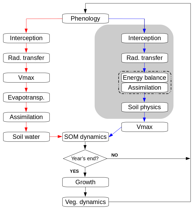
Figure 1Flowchart of the main daily simulation loop in standard LPJ-GUESS (red branch) and the modified version (LPJ-GUESS/LSM, blue branch). The shaded area indicates the sub-daily loop in the modified version. The dashed line encloses coupled iterative calculations.
Radiative transfer in standard LPJ-GUESS is based on Beer's law (Monsi and Saeki, 1953, 2005). The canopy is divided into vertical layers, each absorbing a fraction of the PAR let through by the layer above. The PAR absorbed by each layer is then split among cohorts according to their share of the leaf area index (LAI) in that layer. In this way, taller cohorts have access to more PAR and shade than the lower layers of the canopy. Daily unstressed values of Vmax and canopy conductance gpot are first computed for each cohort assuming well-watered conditions. The actual evapotranspiration rate in the patch is then calculated as the minimum of a potential rate, determined by atmospheric conditions and gpot, and a supply rate, which depends on the amount of soil water available for uptake and the vegetation rooting profiles. For each cohort, the model calculates a daily assimilation rate that is consistent with its contribution to the total patch evapotranspiration. The soil column consists of a top layer of 0.5 m and a bottom layer of 1 m thickness. The fraction of root matter in each soil layer is PFT-specific. Soil water content is updated taking into account daily precipitation, interception, percolation between the two layers, evapotranspiration, and runoff. Daily soil temperature is calculated as a dampened, lagged oscillation around the annual mean of the forcing air temperature, as described in Sitch et al. (2003). More detailed descriptions of the radiative transfer, evapotranspiration, assimilation, and soil organic matter calculations can be found in the Supplement to Smith et al. (2001), Smith et al. (2014), and references therein. The hydrology scheme is described in Gerten et al. (2004).
In the LSM implementation, radiative transfer, energy balance, assimilation, and soil heat and water transport are all solved on a sub-daily basis. Elaborating on Dai et al. (2004), each cohort is conceptualized as two big leaves representing its sunlit and shaded parts. Sunlit leaves receive direct solar radiation and diffuse radiation, while shaded leaves receive only diffuse radiation. The total LAI for each cohort is calculated dynamically by LPJ-GUESS. A stem area index (SAI) was added to account for the impact of stems and branches in the energy balance and radiative transfer calculations. Whole-canopy leaf area and plant area (PAI) indices are obtained by aggregating over cohorts denoted by i:
Based on Kucharik et al. (1998), we set the stem area index of woody PFTs to 10 % of their leaf area index at full leaf coverage. Grasses do not have a stem area index. The sunlit and shaded fractions of leaf and plant area indices are updated in the radiative transfer routine on a sub-daily basis (Sect. 2.2.2).
We replaced the original two-layer soil column with a new profile consisting of nine layers. The top four layers have thicknesses of 7, 10, 13, and 20 cm, in order of increasing depth, and correspond to the top soil layer in the original soil column. The next three layers have thicknesses of 30, 30, and 40 cm and correspond to the original bottom layer. These seven layers constitute the rooting zone. The new water transport scheme assumes, for simplicity, free gravitational drainage at the bottom of the soil column, which can lead to excessive soil dryness during dry periods. Additionally, no heat flux is allowed through the bottom boundary, an approximation better met at higher soil depths. In order to mitigate spurious effects derived from this choice of boundary conditions, we extended the soil column with two additional layers of 50 and 100 cm, reaching a total depth of 3 m.
The sunlit and shaded leaves of each cohort have different assimilation rates and stomatal conductances. The temperatures of sunlit and shaded leaves are different but common to all the cohorts in the patch. The vertical layering of the canopy is kept in the radiation calculations, but the new scheme distinguishes direct and diffuse radiation and two separate wavebands (visible and near infrared). Infrared radiation does not contribute to photosynthetic assimilation but needs to be accounted for in the energy balance calculations. A separate treatment of diffuse and direct radiation allows us to resolve sunlit and shaded leaves. This approach has been shown to lead to predictions of fluxes of energy, water, and CO2 that are comparable in accuracy with those made by more complex, and considerably more computationally expensive, multi-layered canopy models (Wang and Leuning, 1998).
Each cohort exchanges sensible and latent heat with a common canopy air space, which in turn exchanges sensible and latent heat with the atmosphere (Fig. 2). Assimilation and evapotranspiration are calculated consistently in the energy balance routine. Daily averages of absorbed PAR are used to update Vmax for each cohort. The new energy balance, radiative transfer, and soil physics calculations are detailed in Sects. 2.2.1 to 2.2.5.
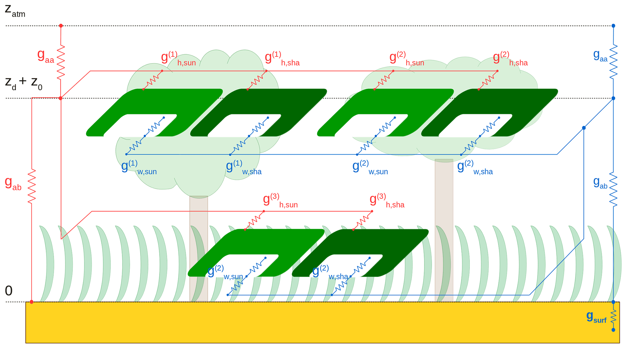
Figure 2Networks of sensible (red) and latent (blue) heat exchange between the ground surface, the canopy, and the atmosphere in the patch. Light green indicates the sunlit fraction of the cohorts, dark green the shaded fraction. gaa is the aerodynamic conductance from the canopy air to the atmospheric reference level (zatm). z0 and zd are, respectively, roughness length and zero plane displacement. gab is the aerodynamic conductance for heat/moisture flux from the ground surface to the canopy air. gsurf is the surface conductance for moisture flux. is the conductance for sensible heat transport from the sunlit (shaded) part of cohort i to the canopy air. is the conductance for moisture transport from the sunlit (shaded) part of cohort i to the canopy air, with the contributions from stomatal conductance and leaf boundary layer conductance represented explicitly. A dry canopy (fwet=0) is represented for clarity.
2.2.1 Energy balance
The energy balance of the patch canopy is described by the following equations (e.g. Bonan, 2015):
where the S terms are absorbed short-wave radiation, L is net emitted long-wave radiation, H is sensible heat flux towards the canopy air space, E is water vapour flux towards the canopy air space, and λ is latent heat of vaporization (here taken to be constant; J kg−1). The sub-indices “sun” and “sha” refer to the sunlit and shaded parts of the canopy. The calculation of the short-wave and long-wave radiation terms is detailed in Sects. 2.2.2 and 2.2.3.
The sensible heat flux from the sunlit part of the canopy to the canopy air space is formulated as
where PAIc,sun is the plant area index of the sunlit canopy, ρ is air density, cP is the specific heat of air at constant pressure, gb is average leaf boundary layer conductance (e.g. Bonan, 2015), Tca is the temperature of the canopy air, and Tsun is the temperature of the sunlit canopy. The factor 2 expresses heat loss from both sides of the leaf and stem elements.
The latent heat flux from the sunlit part of the canopy to the canopy air is
where qca is the specific humidity of the canopy air, q∗(Tsun) is the specific humidity inside the stomatal cavity, taken to be the saturated humidity at the leaf temperature, and gw,sun is the conductance for water vapour flux from the sunlit part of the canopy to the canopy air space. The latter is calculated as a weighted average of the contributions from evaporation of intercepted water and transpiration through the stomata (Appendix A):
In this equation fwet is the wet fraction of the canopy, the factor ηsun limits evaporation to the amount of intercepted water present in the canopy, and is the leaf area index of the sunlit part of cohort i. The stomatal conductance of the sunlit leaves of cohort i, , is related to the leaf-level net photosynthetic rate through a semi-empirical model. We implemented two selectable stomatal conductance models: the Ball–Berry model (Ball et al., 1987) and the Medlyn model (Medlyn et al., 2011). Equations analogous to Eqs. (5) through (7) apply to the shaded part of the canopy.
The energy balance equation for the ground surface is
where G is heat conducted into the ground. The sensible heat from the ground surface to the canopy air space is
where gab is the aerodynamic conductance from the ground surface to the canopy air space, which is calculated following Sakaguchi and Zeng (2009). The latent heat from the ground surface to the canopy air is given by
where we used the model of Sakaguchi and Zeng (2009) for the surface conductance gsurf, and αq∗(Tg) is the specific humidity of the air at the ground surface (Philip, 1957).
The heat conducted into the ground is calculated as
where , , and Δz(1) are, respectively, the thermal conductivity, the temperature, and the thickness of the top soil layer.
The following two equations express conservation of latent and sensible heat:
where H↑ and λE↑ are, respectively, the sensible and latent heat fluxes into the atmosphere, given by
Here, Tatm and qatm are the temperature and specific humidity of the air at the atmospheric reference level, and gaa is the aerodynamic conductance above the canopy. The latter is calculated by applying the Monin–Obukov similarity theory (see e.g. Bonan, 2015), which requires knowledge of the surface roughness length, z0, and the zero plane displacement, zd. These are calculated as a function of the canopy plant area index, PAIc, and the canopy height, hc, according to the model of Raupach (1994, 1995):
where k=0.4 is the von Karman constant and . Canopy height is calculated, following Forrest et al. (2020), as an average of cohort heights weighted by their foliar projective cover (FPC).
Equations (3), (4), and (8), subject to constraints (12) and (13), are solved simultaneously every time step with a multidimensional Newton–Rhapson method (e.g. Press, 2003).
2.2.2 Short-wave radiative transfer
We adapted the two-big-leaf model of Dai et al. (2004), based on the two-stream model of Dickinson (1983) and Sellers (1985), to LPJ-GUESS's multiple-cohort, vertically layered canopy. This approach considers direct solar radiation and diffuse atmospheric radiation separately. The intensity of the direct solar radiation beam in the canopy decreases exponentially with cumulative plant area index P (measured from the top of the canopy, increasing downwards) (Monsi and Saeki, 1953, 2005):
where is incoming direct solar radiation and k is the direct-beam extinction coefficient. The profile of diffuse radiation in the canopy results from the multiple scattering and backscattering of incoming radiation by leaves and stems. Corrected profiles (normalized by incoming radiation) of scattered direct-beam ( and ) and scattered atmospheric diffuse radiation ( and ) are given in analytic form in Dai et al. (2004) (the arrows indicate the direction of propagation).
The direct-beam radiation absorbed in a canopy layer l between P and P+ΔlP is calculated as the fraction of the decrease in direct-beam intensity in that layer that is not scattered:
where ω is the direct-beam scattering coefficient, and Δl denotes change across layer l. The diffuse radiation absorbed in the layer is the sum of the radiation from the direct beam that is scattered and reabsorbed in the layer and the contribution from the diffuse beams:
where is incoming atmospheric diffuse radiation. The radiation absorbed by the sunlit and shaded parts of this layer is
where the sunlit and shaded fractions of the layer are given by
The total amount of short-wave radiation absorbed by the sunlit and shaded parts of the canopy is obtained by summing over layers:
The short-wave radiation absorbed by the ground surface is calculated as the difference between the downward and upward beams at P=PAIc:
The short-wave radiation reflected back at the atmosphere is obtained by evaluating the upward beams at P=0:
The optical elements in the canopy have different properties in the visible and near-infrared wavebands, so the equations above are applied separately to these two parts of the spectrum, and the contributions are summed to calculate total absorption. In order to keep the model development process tractable, we set the optical properties of the canopy to the following values, regardless of PFT:
where α is absorptivity, τ is transmissivity, “vis” refers to visible radiation, and “nir” refers to near-infrared. These values were taken from the ones assigned to tropical trees by Oleson et al. (2010). Soil albedo is calculated from the soil dry- and moisture-saturated reflectances and the water content of the top soil layer following Oleson et al. (2010). Soil colour classes are from Lawrence and Chase (2007) and were obtained from the dataset included in the CLM4.0 code (Lawrence et al., 2011).
The PAR absorbed by the sunlit leaves of a cohort i is obtained as the sum over layers of the absorbed visible radiation weighted by the cohort's fractional leaf area index in each layer:
The sunlit leaf and plant area indices of cohort i are obtained by aggregating over layers:
The sunlit plant area index for the whole canopy is calculated by summing over cohorts:
Equations analogous to Eqs. (33) to (36) apply to the shaded parts of the canopy.
2.2.3 Long-wave radiative transfer
The long-wave radiation emitted by the sunlit part of the canopy is (Dai et al., 2004)
where σ is the Stefan–Boltzmann constant, L↓ is the incoming atmospheric long-wave radiation, Tsun, Tg is expressed in Kelvin, and
The thermal emissivity of plants and soil is assumed to be 1. The net emission of long-wave radiation by the shaded part of the canopy is described by analogous equations.
The long-wave radiation emitted by the ground surface is
The bulk long-wave radiation emitted by the land surface toward the atmosphere is
2.2.4 Assimilation and stomatal conductance
In what follows, variables that are updated daily are denoted with the subscript “day”. Daytime averages are denoted with the subscript “dt”. All the other variables are computed on a sub-daily basis. Photosynthetic assimilation is now calculated within the sub-daily energy balance routine (Fig. 1). A net photosynthetic rate is computed for the sunlit and shaded leaves of each cohort separately by calling the photosynthesis routine built in LPJ-GUESS. This calculation is based on the biochemical model of Collatz et al. (1991, 1992), the strong-optimality model of light use efficiency at the canopy level of Haxeltine and Prentice (1996), and the nitrogen limitation of the maximum carboxylation rate introduced in Smith et al. (2014). The net photosynthetic assimilation is accumulated over the diurnal cycle and subtracted from heterotrophic respiration (Rh, computed daily) to calculate daily net ecosystem exchange (NEE).
For a given cohort i, the maximum carboxylation rate, , is recalculated at the end of every simulation day and depends linearly on the total amount of daily absorbed photosynthetic active radiation, (Haxeltine and Prentice, 1996):
In this equation, is expressed per unit patch area. The slope of the relationship, fv, encodes the influence of temperature and nitrogen limitation. The calculation of uses the original LPJ-GUESS PAR absorption estimation as described in Sect. 2.2. However, the influence of temperature is calculated using the newly simulated canopy temperature rather than the daily average air temperature. Updating on sub-daily timescales is not necessary because readjustment of leaf nitrogen content and photosynthetic traits occurs on timescales of days to weeks (e.g. Reich et al., 1991; Irving and Robinson, 2006) and therefore cannot follow diurnal environmental variations.
The daytime averaged leaf temperature, , is weighted by the daily-averaged fractions of sunlit and shaded leaves for cohort i:
where ndt is the number of daytime sub-daily periods.
Separating the contributions to daily absorbed PAR from sunlit and shaded leaves, maximum carboxylation rates for the sunlit and shaded parts of the cohort are estimated as
where and are the total daily PAR absorbed by the sunlit and shaded leaves of cohort i, respectively. Combining Eqs. (41) and (43) yields, for sunlit leaves,
The maximum carboxylation rate per unit leaf area is then calculated as
where is the daily-averaged sunlit LAI of cohort i, and we have introduced a factor β to limit the photosynthetic rate under conditions of water stress. The prefactor 86 400−1 converts the rate from d−1 to s−1. Analogous equations apply to shaded leaves.
The water stress factor β is formulated as a sum over soil layers of a water uptake response function weighed by a PFT-specific vertical rooting profile:
where r(j) is the fraction of roots in soil layer j. In order to study the impact of the β factor on the model predictions, we implemented four different options for the water uptake response function . In the Noah type (Niu et al., 2011), decreases linearly in each soil layer with volumetric water content θ(j) down to the wilting point:
where θwilt and θfc are volumetric water content at wilting point and field capacity, respectively. In LPJ-GUESS, the wilting point is assumed to be at a matric potential of m, and the corresponding soil water content is calculated following Prentice et al. (1992).
The CLM-type water uptake response function is formulated in terms of matric potential (Oleson et al., 2010):
where ψ(j) is the matric potential of layer j, ψsat is the matric potential at saturation, and ψwilt,CLM is the matric potential at wilting point, set to −150m. In this case, the water uptake response is flatter than in the Noah-type case when the soil is wet, and decreases more steeply when the soil gets drier. We also implemented a modified version of the CLM-type uptake function, with the same functional form but using LPJ-GUESS's −45m wilting matric potential instead of CLM's −150m.
The SSiB type water uptake response function is
where the parameter c2 depends on PFT, and takes values between 4.36 and 6.37 (Xue et al., 1991). In this study, we set c2 to a fixed value of 5.8 for all PFTs, which results in high β values in most of the water availability range, and a steep decrease when approaching the wilting point.
Figure 4 shows the behavior of the different formulations of as a function of volumetric water content. This type of formulations, which are widely used in LSMs (see Damour et al., 2010, for an overview), are phenomenological relationships that attempt to capture the response of plants to water stress in a rather simplified way (Egea et al., 2011; De Kauwe et al., 2013). Transpiration of soil water by plants is primarily driven by the water potential gradient along the soil–plant–atmosphere continuum. Plants regulate this gradient by opening and closing their stomata in response to environmental factors, including vapour pressure deficit, leaf water potential, and soil water availability, in a way that depends on their hydraulic strategy (a detailed discussion can be found in Lambers et al., 2008). Including a more explicit representation of soil–plant–air hydraulics as well as physiological constraints in an LSM leads to better agreement with observations than the above formulations under soil water stress conditions (Bonan et al., 2014). However, implementing these more complex formulations in ESMs remains a challenge due to a lack of data for broader applicability and computational efficiency tradeoffs (Clark et al., 2015).
Stomatal conductance and photosynthetic rate are related through a semi-empirical model. The photosynthesis rate depends on the CO2 concentration inside the stomatal cavity. This concentration is related to the atmospheric CO2 concentration through a diffusion process across the stomatal opening and the leaf boundary layer and therefore depends upon stomatal conductance, which in turn depends on the photosynthetic rate. Hence, photosynthetic rate and stomatal conductance are calculated simultaneously by iteration. A detailed description of the algorithm can be found in Bonan (2019).
As noted above, we implemented two selectable stomatal conductance models. In the Ball–Berry model (Ball et al., 1987), stomatal conductance depends linearly on net assimilation and the fractional humidity at the leaf surface hs, and inversely on CO2 concentration at the leaf surface, cs. The stomatal conductance for sunlit leaves of cohort i is
where is the net photosynthetic rate per unit leaf area, gmin is a minimum stomatal conductance, and g1 is a PFT-specific parameter. The Medlyn model (Medlyn et al., 2011) is derived from the assumption that stomata optimize CO2 uptake while minimizing water loss. In this model, stomatal conductance depends inversely on the square root of the vapour pressure deficit at the leaf surface, Ds. The stomatal conductance for sunlit leaves of cohort i is
Values of the parameters g1,BB and g1,Med for specific PFTs were obtained following Sellers et al. (1996) for the Ball–Berry model and De Kauwe et al. (2015) for the Medlyn model. Figure 3 shows the different behaviour of the stomatal conductance models as a function of Ds.
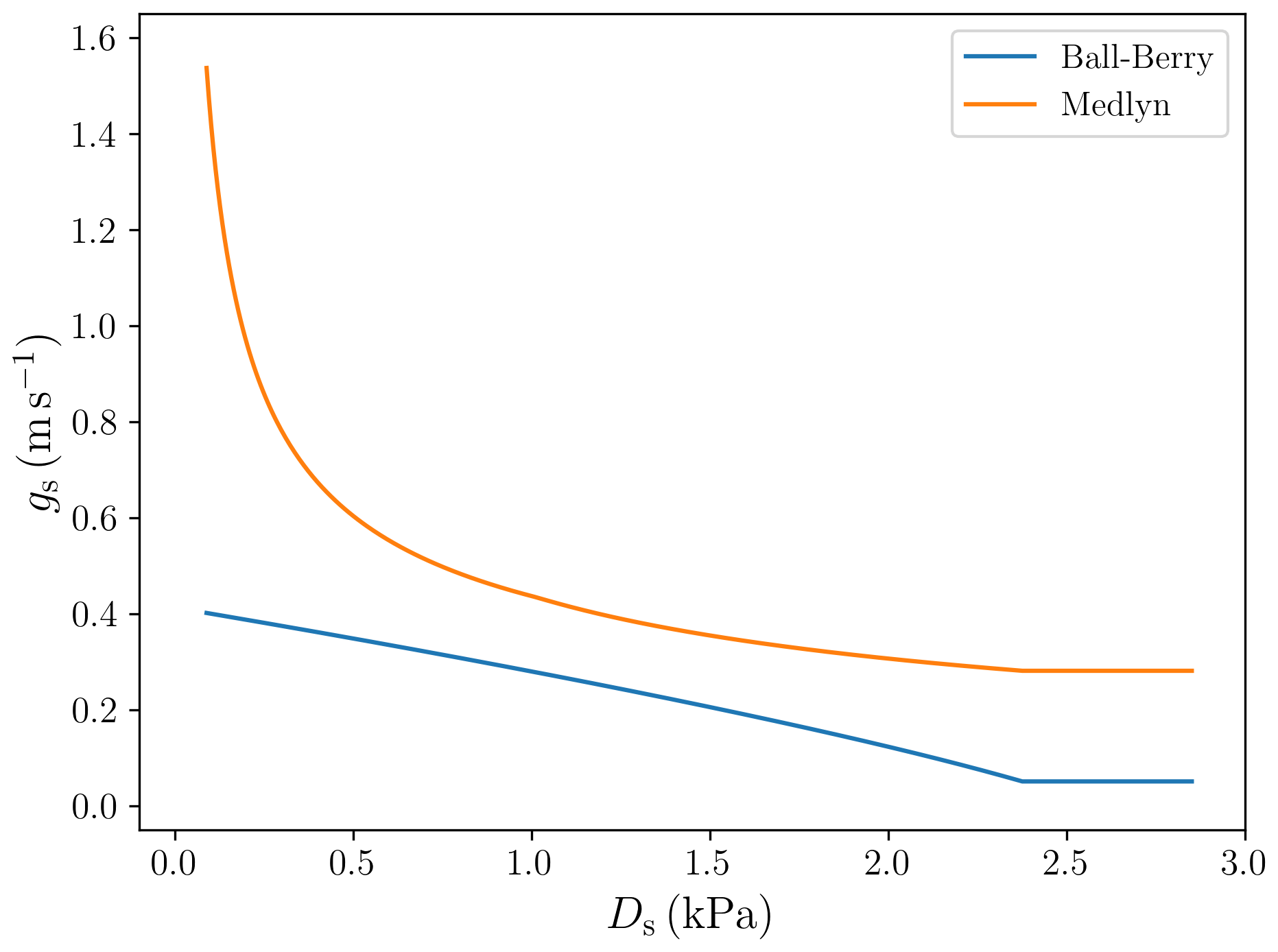
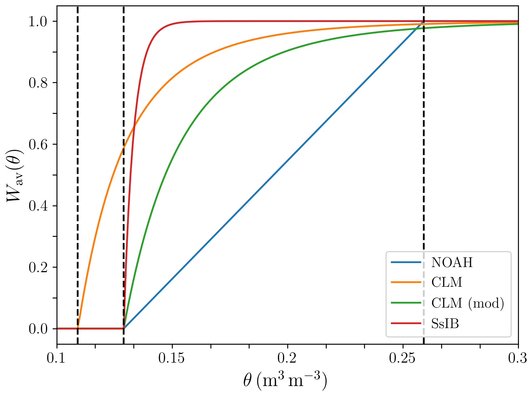
Figure 4Factor limiting plant water uptake as a function of volumetric soil water content. The dashed vertical lines represent, from left to right, the volumetric soil water content at a wilting matric potential of −150 m, at a wilting matric potential of −45 m, and at field capacity.
2.2.5 Soil physics
In standard LPJ-GUESS, soil temperature is used in calculations related to ecosystem respiration and nitrogen cycling, while soil water content influences plant water uptake and evapotranspiration. Both quantities affect soil organic matter decomposition rates.
Soil temperature Ts is now calculated by solving the heat transport equation:
where ch(z) and κs(z) are soil heat capacity and thermal conductivity, respectively. The top boundary condition is given by the heat flux into the ground, G, calculated in the energy balance routine (Eq. 11). Heat flow through the bottom boundary of the soil column is neglected. Thermal conductivity is calculated following the method of Johansen (1977). Soil heat capacity is computed as a weighted sum of the heat capacities of the dry soil, which depends on soil texture, and water (de Vries, 1963). Soil organic matter does not contribute to soil heat capacity in the current version of the model.
Vertical water transport in the soil column is described by the Richards equation (Richards, 1931), which can be expressed in the following form:
Here, θ is volumetric water content, λw(θ) is hydraulic diffusivity, γw(θ) is hydraulic conductivity, and Sθ(z) is a volumetric sink term that accounts for plant water uptake (Sθ≤0). Hydraulic diffusivity and conductivity are calculated as a function of soil texture and soil water content by using the expressions derived by Clapp and Hornberger (1978) and Cosby et al. (1984). Rainwater that is not intercepted by the canopy infiltrates into the soil at a rate limited by the soil's infiltration capacity as given by the Green–Ampt equation (Green and Ampt, 1911). Free gravitational drainage is assumed at the bottom of the soil column.
Soil temperature, water content, ecosystem respiration, plant water uptake and evapotranspiration are calculated in the sub-daily loop. Equations (52) and (53) are solved with a Crank–Nicolson scheme (e.g. Press, 2003). Daily averages of water content and temperature over the layers corresponding to standard LPJ-GUESS top and bottom layers are then used as inputs to the original soil organic matter and nitrogen cycling routines.
3.1 Model verification
The revised model was verified by performing energy and water conservation tests. At any given time step, the energy conservation error per unit time and per unit patch area, Δuerr (), is calculated as
where 〈⋅〉 indicates an average over patches, and Δusoil is the rate of change of energy stored in the soil column per unit patch area. The latter is calculated as
where Δt is the time step in seconds, and , Δz(j) and are, respectively, the heat capacity, thickness and temperature of soil layer j. Figure 5 shows the frequency of the energy conservation error relative to the energy input to the system (i.e. the total incoming irradiance, ). The vast majority of the time steps (∼99.8 %) the error is smaller than 0.2 % of the incoming radiation, and the error is never larger than 0.85 % of the energy input. The mean energy balance closure error is ∼0.013 % of the energy input (σ∼0.035 %).

Figure 5The histogram shows the energy conservation error, as a percentage of the energy input, incurred at every time step. The symbols indicate the mean absolute error corresponding to each bin. The error bars indicate ±1σ around the mean. The plots are derived from data from the historical period of all LSM simulations in this study.
The water conservation error is computed as
where P is precipitation, R is runoff (including surface runoff and base flow), E↑ is evapotranspiration, Δwsoil is the change in soil water content per unit patch area, per unit time, and Δwc is the change in canopy water content. This error is, on average, % of the precipitation at any given time step (), and never surpasses % of the water input.
We therefore conclude that the magnitude of the errors in energy balance closure and water conservation are negligible.
3.2 Evaluation set-up
We evaluated the revised model by comparing hourly and monthly simulated fluxes of sensible and latent heat and annual CO2 fluxes, with flux tower measurements from 21 FLUXNET2015 (Pastorello et al., 2020) sites. The current version of the model does not simulate snow or frozen soil water, so we restricted our study to sites where the air temperature remained above 0 ∘C throughout the measuring period. We additionally discarded wetland sites, which require a more detailed representation of soil water and groundwater hydrology (Wania et al., 2009). A list of the selected sites is presented in Table 2. The locations of the sites are represented on the world map in Fig. 6.
Table 1List of plant functional types in the standard configuration of LPJ-GUESS (only PFTs predicted by the simulations in this study are listed).
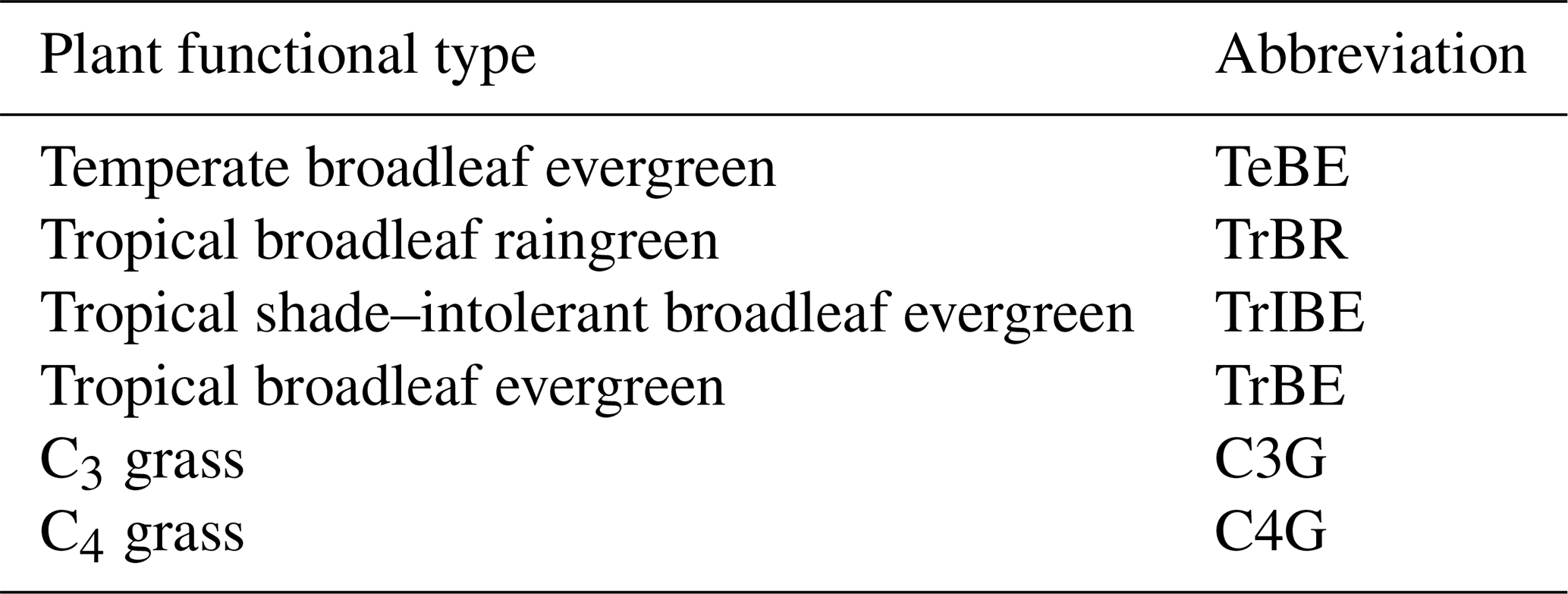
Table 2Brief description of selected sites. The land cover classification was taken from the FLUXNET site description web pages. The reference level height is taken as the height of the measuring sensors above the canopy. A dash indicates that we were not able to find an observed LAI value for the site.
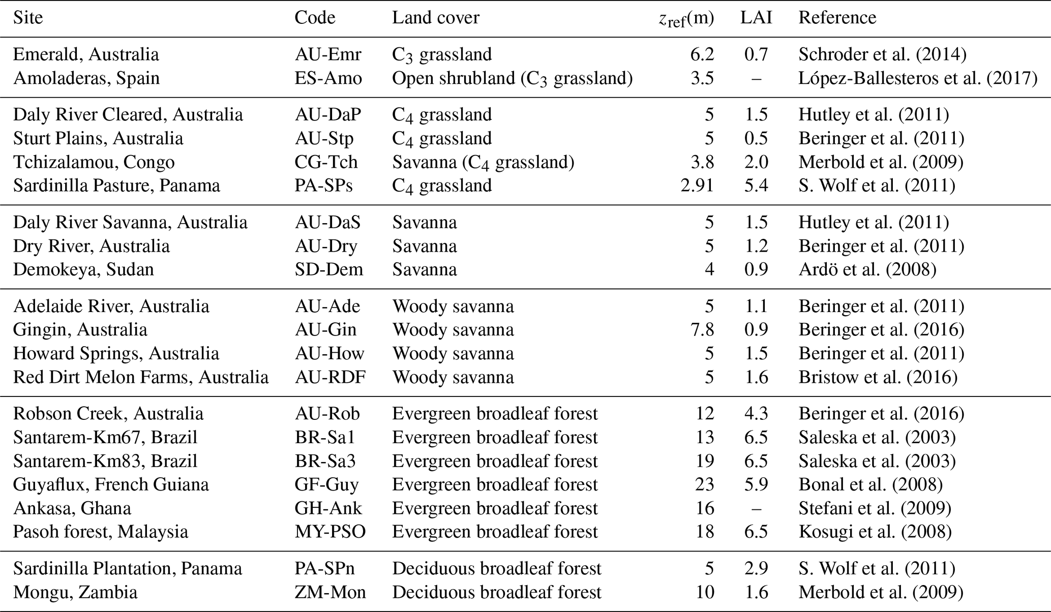
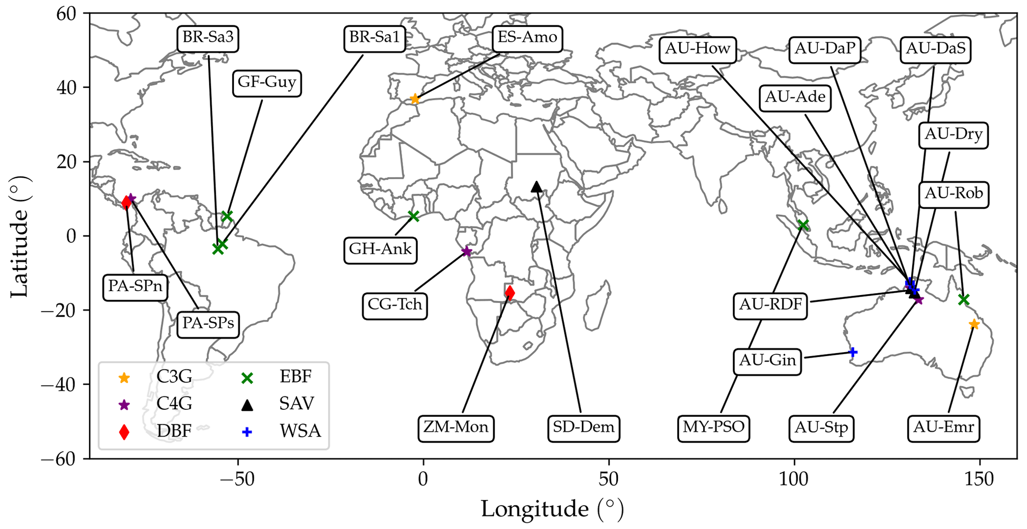
Figure 6FLUXNET sites selected for model evaluation. Different symbols indicate different land cover types. The sites are labelled according to their site code (Table 2).
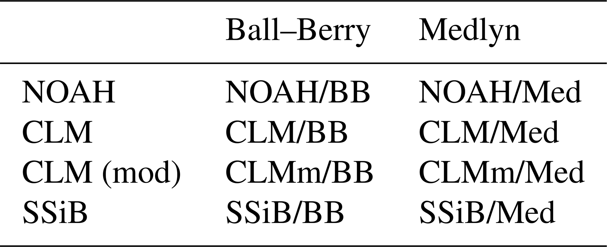
For each site, we ran eight simulations, covering all possible configurations of the water uptake response functions and stomatal conductance schemes described in Sect. 2.2.4 (Table 3). We used the climate data collected at the tower sites to force the model. Half-hourly forcing data were converted to hourly averages to use a fixed time step of 1 h in all simulations. We set a lower boundary of 10 % of the dataset median on the air humidity to correct for physically invalid negative values. Nitrogen deposition data are from Lamarque et al. (2013). The soil texture data used to calculate soil hydraulic and thermal properties (as described in Sect. 2.2.5) at each site were as in Sitch et al. (2003), based on the Digitized Soil Map of the World (Zobler, 1986; FAO, 1991). Atmospheric CO2 concentration data are from McGuire et al. (2001). Additionally, we ran a standard (non-LSM) LPJ-GUESS simulation to compare both model versions' predictions of monthly evapotranspiration and a number of ecosystem composition and function variables. The number of replicate patches was set to 100 in all the simulations to avoid spurious effects of the stochastic ecosystem processes on the modelled fluxes. Simulation of wildfires was switched off in all simulations.
Table 3Summary of the LPJ-GUESS/LSM simulations carried out. Simulations with different stomatal conductance schemes are arranged in columns: Ball–Berry (BB) and Medlyn (Med). Simulations with different water uptake response function types are arranged in rows: NOAH, CLM, modified CLM, and SSiB.
All natural PFTs were allowed to establish in forest and savanna sites. Since the focus of the model evaluation was placed on the turbulent fluxes, we restricted the simulated PFTs to grassy types at sites classified as grasslands, which limits modelled surface roughness. This was also done for Spain-Amoladeras and Congo-Tchizalamou. Amoladeras is classified as an open shrubland on the FLUXNET reference, but the vegetation is short and the most abundant species is Machrocloa Tenacissima, a type of grass (López-Ballesteros et al., 2017). Tchizalamou, which is classified as savanna, is actually a C4 grassland (Merbold et al., 2009).
The simulations were spun up from a bare ground state following a standard procedure that combines 500 simulation years with a semi-analytic calculation of the equilibrium size of the soil organic matter pools (see Supplement), to bring C and N soil and vegetation pools to near equilibrium with the climate. During the spin-up phase, the site climate spanning the whole measurement period was repeated cyclically, with interannual trends in air temperature removed, and the atmospheric CO2 concentration was kept at the level of the first year of observations at each site.
3.3 Analysis
Half-hourly measured fluxes were converted to hourly averages for direct comparison with model outputs. Sub-daily FLUXNET data are classified into four quality categories: 0 (measured), 1 (good-quality gap fill), 2 (poor-quality gap fill), and 3 (downscale from ERA reanalysis data). In our analysis, we only used sub-daily fluxes with a quality flag of 0 or 1. For monthly and annual fluxes, the quality flag varies between 0 and 1 and indicates the fraction of the sub-daily values in that month/year whose quality is either 0 or 1. We only used monthly and annual fluxes with a quality flag equal to or greater than 0.75. Following Stöckli et al. (2008), we further discarded fluxes with friction velocity m s−1 in order to avoid possibly biased eddy covariance measurements during periods of weak turbulence (Schroder et al., 2014).
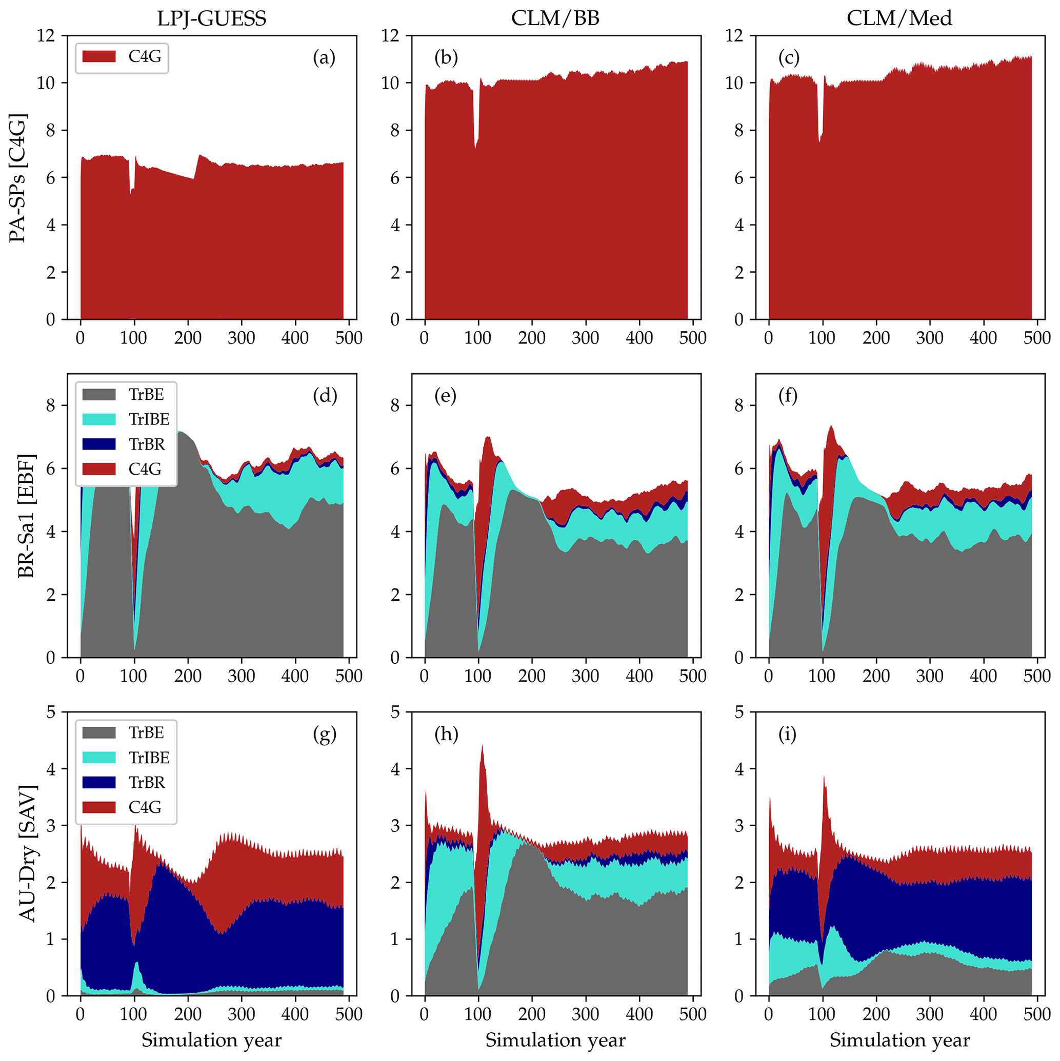
Figure 7LAI values for the spin-up period at three selected sites: PA-SPs (panels a–c), BR-Sa1 (panels d–f), and AU-Dry (panels g–i). The columns correspond to standard LPJ-GUESS (a, d, g), CLM/BB (b, e, h), and CLM/Med (c, f, i) simulations. The time series were smoothed for better visualization by applying a 15-year running average.
To evaluate the agreement between measured and simulated turbulent heat fluxes at each site for all different model configurations we used standard statistical metrics: correlation coefficient (r), mean bias, and root mean square error (RMSE). We also considered the standard deviation of the modelled fluxes normalized by the standard deviation of the observed fluxes (), which provides a measure of the agreement between observed and simulated variability.
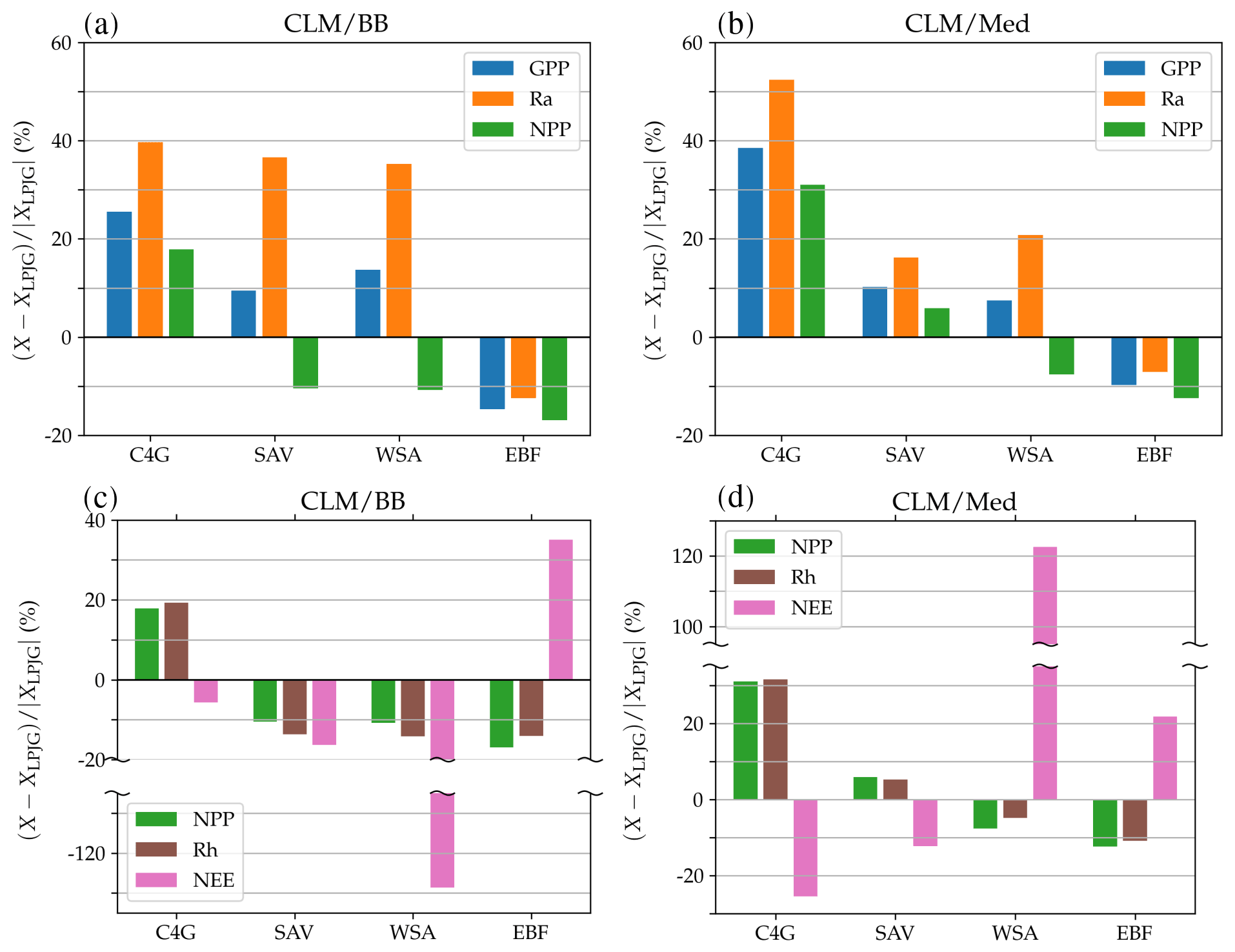
Figure 8Panels (a, b): percent change in average gross primary production (blue), autotrophic respiration (orange), and net primary production (green), simulated by the LSM version with respect to standard LPJ-GUESS. Panels (c, d): percent change in predicted average net primary production (green), heterotrophic respiration (brown), and net ecosystem exchange (pink).
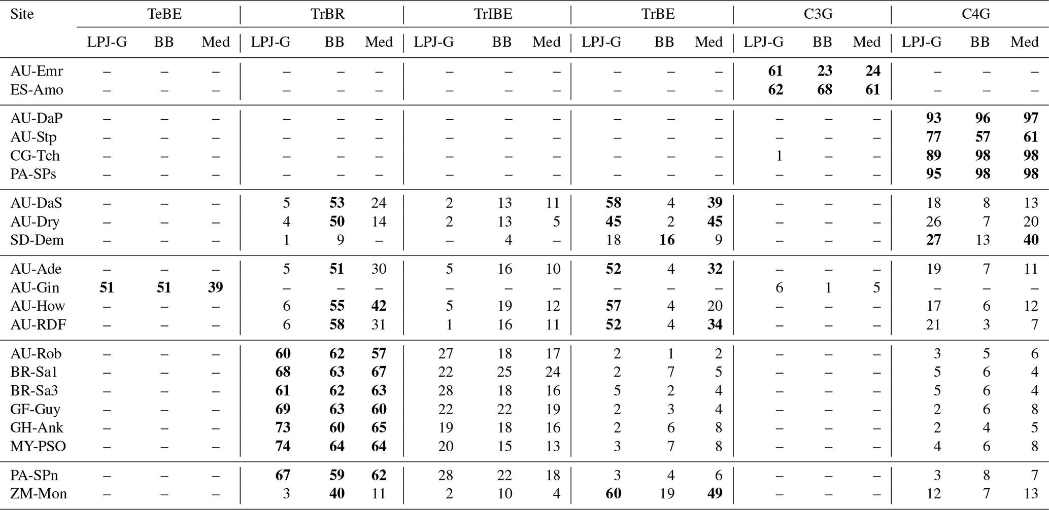
Table 4Foliar projective cover, averaged over the whole simulated period, of the plant functional types predicted for each site, given as a percentage. The LSM simulations use the CLM-type water uptake response factor. The dominant PFT for each site is highlighted in bold font.
3.4 Results
3.4.1 Ecosystem composition and function
The emerging ecosystem composition in both LSM runs is similar to the standard LPJ-GUESS prediction over forests and grasslands, but it is sensitive to the choice of stomatal conductance scheme at some savanna and woody savanna sites and at ZM-Mon (Table 4). Figure 7 shows the LAI evolution of the established PFTs over the spin-up period for the CLM/BB, CLM/Med, and standard LPJ-GUESS simulations at three selected sites. All three simulations predict a C4 grassland at PA-SPs, but LAI values are much higher in the LSM simulations (∼11) than the LPJ-GUESS prediction (∼6.5). At BR-Sa1 (a tropical rainforest), the species composition is similar for the three simulations, but LAI values are lower in the LSM runs (∼5.5 vs. ∼6.2). At AU-Dry, the use of different stomatal conductance schemes causes a shift in PFT composition. The BB simulation favours evergreen trees, while the PFT mix is dominated by raingreen trees in the Med simulation, a prediction closer to standard LPJ-GUESS. We found this behaviour to be representative of how the soil water uptake response factor and the stomatal conductance scheme influence the PFT composition at most savanna and woody savanna sites in the LSM simulations. A stronger limitation on transpiration (e.g. the NOAH-type water uptake response factor or the Ball–Berry stomatal conductance model) results in higher soil water content throughout the year, which promotes stronger growth of evergreen trees.
Model predictions for the rest of the selected variables are shown in Table 5. The two C3 grassland sites show different behaviour with respect to ecosystem productivity and respiration. At AU-Emr, LSM simulations predict substantially lower gross primary production (GPP) and autotrophic respiration (Ra) than standard LPJ-GUESS, which results in lower estimates of net primary production (NPP). This site is a net carbon source (positive NEE) in all three simulations, which agrees with observations. At ES-Amo, the NPP increase in the LSM runs is larger than the decrease in heterotrophic respiration (Rh), resulting in an enhanced carbon sink compared with standard LPJ-GUESS.
Table 5Comparison of selected variables related to simulated ecosystem structure and function between standard LPJ-GUESS and the LSM version at the selected sites. The LSM values are from the CLM/BB and CLM/Med simulations. Gross primary production (GPP), autotrophic respiration (Ra), net primary production (NPP), heterotrophic respiration (Rh), and net ecosystem exchange (NEE) are given in . Bold fonts in the LAI and NEE columns indicate the closest match to the observed value. Bold fonts in the rest of the columns indicate the LSM prediction closest to standard LPJ-GUESS.
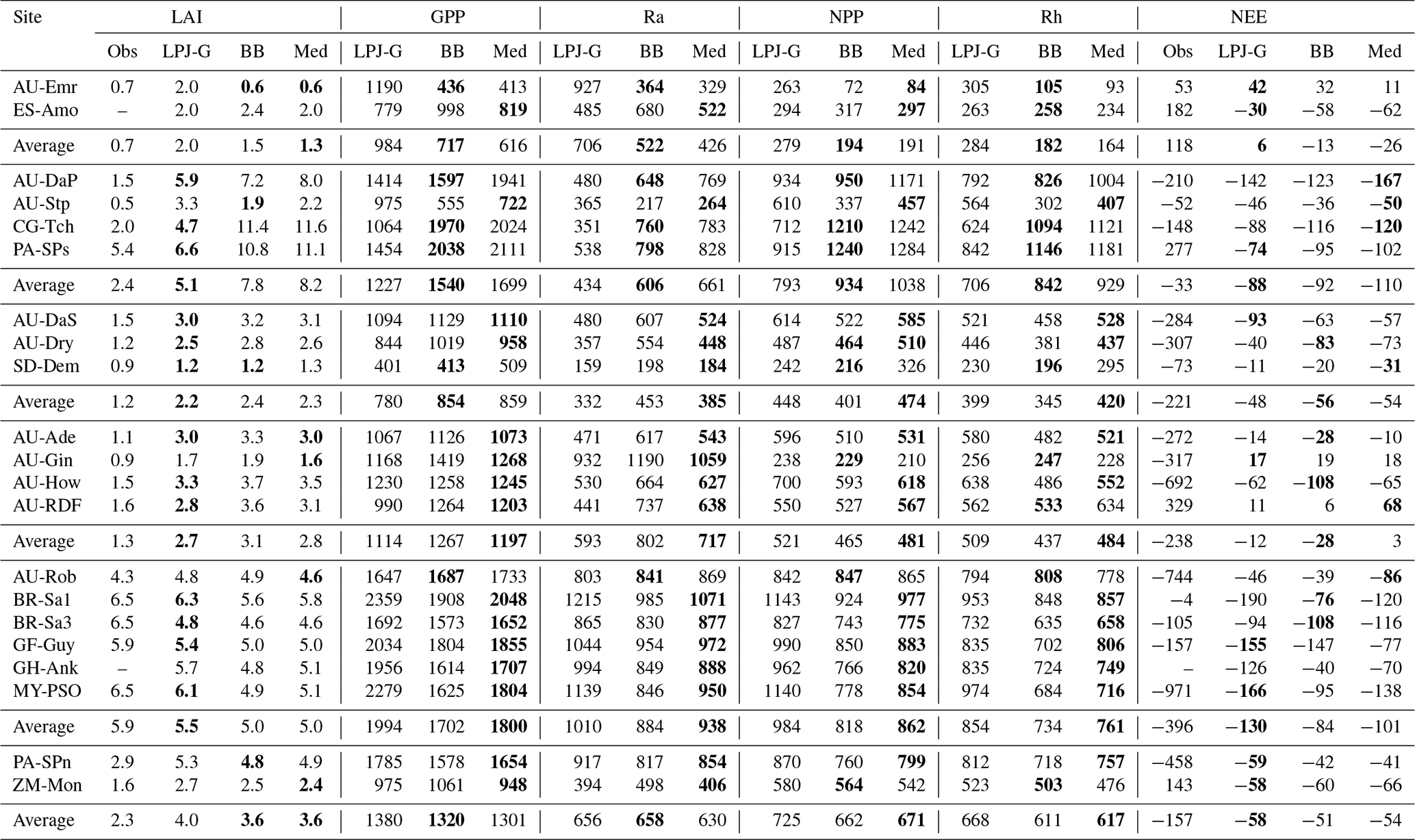
At PA-SPn, both NPP and Rh decrease in the LSM simulations, but the former decreases less than the latter, resulting in slightly weaker carbon sinks in the LSM simulations. The three simulations predict carbon fluxes much smaller than the measured value of −458 . Predictions for ZM-Mon show some differences between runs, but NPP and Rh are similar in all three simulations, resulting in carbon sinks of . This result is inconsistent with measurements at the site, which indicate a carbon source of 143 .
Differences in simulated carbon fluxes between standard LPJ-GUESS and the CLM/BB and CLM/Med runs for the remaining land cover types are summarized in Fig. 8. Both LSM runs predict, on average, higher GPP and Ra values than the non-LSM simulation over C4 grassland, savanna, and woody savanna sites. This results in an increased average NPP value in C4 grasslands (∼18 % in the CLM/BB run and ∼31 % in the CLM/Med run) and a decreased average NPP at woody savanna sites ( % and % in the CLM/BB and CLM/Med runs, respectively). At savanna sites, the increase in GPP in both LSM simulations is similar (∼10 %), but the increase in Ra is much higher for CLM/BB, which leads to changes in NPP of % in the CLM/BB run and ∼6 % in the CLM/Med run. At forest sites, the balance between decreased values of GPP and Ra results in lower NPP values in the LSM simulations. Average values of Rh in the CLM/BB simulation increase over C4 grasslands and decrease over woody savannas and evergreen forests. The CLM/Med simulation shows the same pattern except over savanna sites, where Rh increases by ∼5 % with respect to standard LPJ-GUESS. Over woody savannas, the average NEE change is % for the CLM/BB run and ∼122 % for the CLM/Med run.
The above-described discrepancies between standard LPJ-GUESS and the LSM versions stem from the different physical environments simulated in the models. Calculating assimilation at the newly simulated canopy temperature, rather than the air temperature, can lead to either higher or lower productivity, depending on the optimal photosynthetic temperature ranges of each PFT and the impact of temperature on nitrogen limitation (Sect. 4.2). Canopy temperature also affects autotrophic respiration, while differences in the simulated soil humidity and temperature impact organic matter decomposition rates and heterotrophic respiration. The combination of these effects results in differences in simulated carbon and nitrogen pools and NEE (we have included a comparison between soil carbon and nitrogen pools simulated by standard LPJ-GUESS and LPJ-GUESS/LSM in the Supplement).
The large relative changes in NEE between simulations result from small discrepancies in magnitude. Figure 9 shows a comparison between land cover averages of measured and modelled NEE for C4 grasslands, savanna, woody savanna, and evergreen forests. Average measured NEE is negative for all land cover types and substantially more negative than in the simulations for savanna, woody savanna, and evergreen broadleaf forests, implying an average underestimation of the C sink by the models at these sites. At C4 sites simulations predict NEE values between −88 and −110 , while observations indicate a less negative value of −33 . For savanna, measured NEE is −221 , while simulations predict an average between −48 and −56 . For woody savanna, measured NEE averages to −238 , while simulated fluxes range between −28 and 3 . Simulated fluxes at evergreen broadleaf forests are, on average, between −84 and −130 , while measurements indicate an average NEE of −396 . However, this is the result of very large negative values measured at AU-Rob and MY-PSO (Table 5). In general, differences in simulated fluxes between standard LPJ-GUESS and the LPJ-GUESS/LSM simulations are small compared with the magnitude of observed fluxes, and the interannual and cross-site variabilities of the measured fluxes are much greater than in the simulations. The discrepancies between observed and simulated NEE magnitude and variability reflect the fact that, in the simulations, the carbon pools are all close to equilibrium with the climate and atmospheric CO2 concentration as a result of the spin-up procedure described in Sect. 3.2. Differences between observed and simulated NEE values are to be expected because we did not attempt to reproduce site history, including age, disturbance, and legacies arising from historical trends in CO2 concentration.
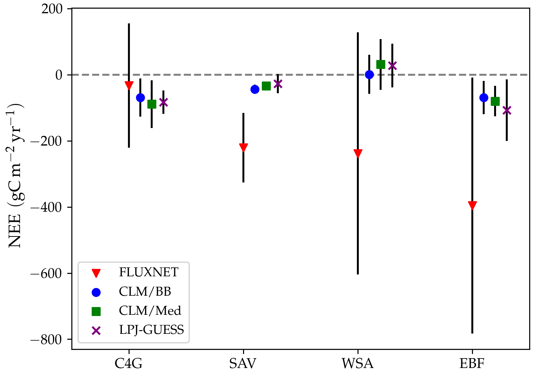
Figure 9Comparison between observed and modelled annual NEE. The symbols indicate averages over sites with the same land cover type. Red triangles correspond to flux tower CO2 measurements. Blue dots, green squares, and purple crosses correspond, respectively, to the CLM/BB, CLM/Med, and standard LPJ-GUESS simulations. The bars represent 1 standard deviation above and below the average.
3.4.2 Annual and diurnal cycles of turbulent heat fluxes
Figure 10 shows examples of simulated and observed monthly averages of turbulent and latent heat fluxes over the course of a year at four sites: Gingin (AU-Gin), Daly River Savanna (AU-DaS), Santarem-Km67 (BR-Sa1), and Guyaflux (GF-Guy). Examples of the monthly-averaged diurnal cycle for the same sites are shown in Figs. 11 and 12. We chose these sites and years to illustrate situations with varying degrees of agreement between simulations and measurements. The simulated fluxes are from the run using the CLM-type water uptake response function and the Medlyn model of stomatal conductance (CLM/Med).
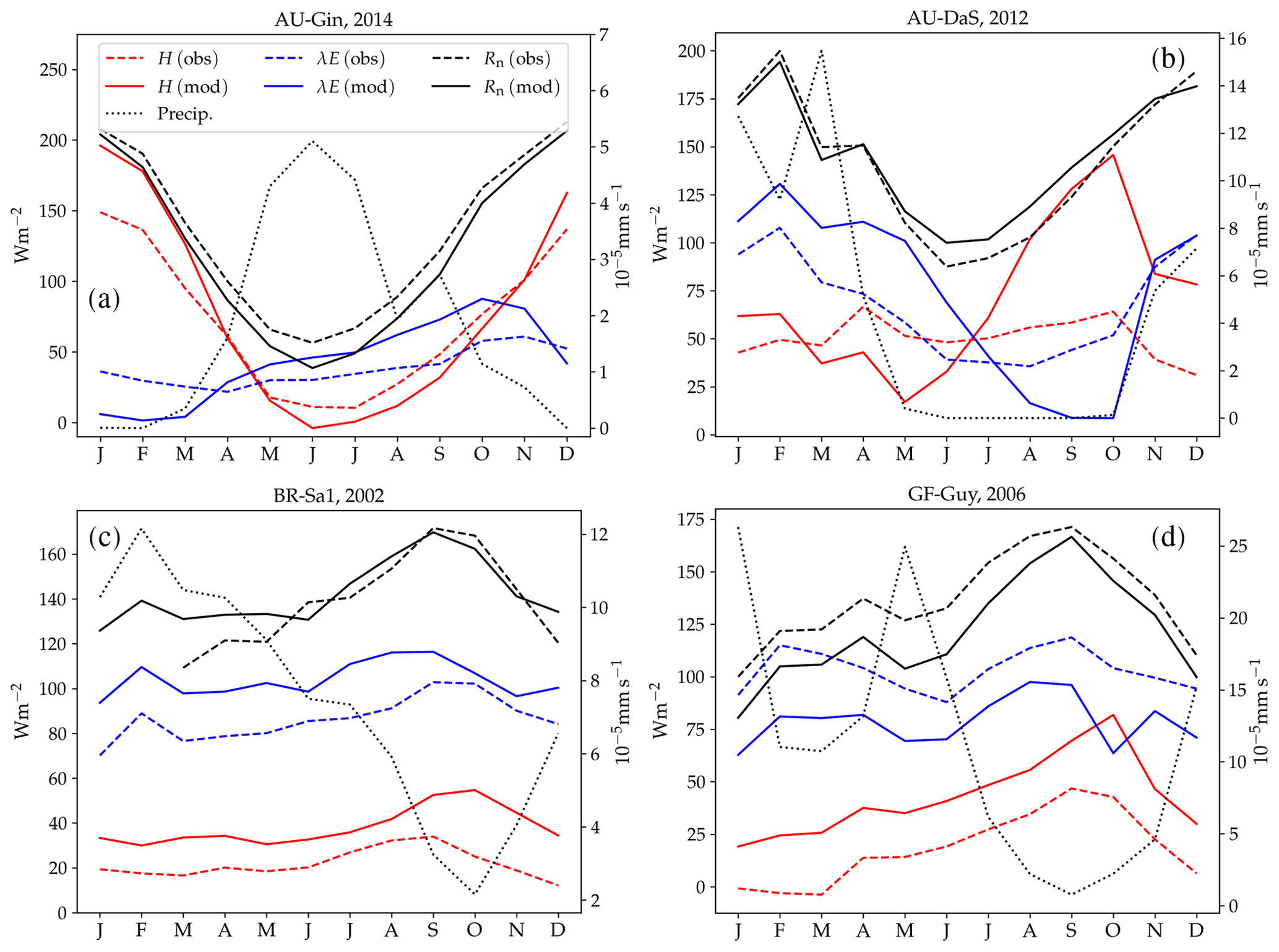
Figure 10Observed and simulated annual cycles of sensible (H) and latent (λE) heat flux at four selected sites: Gingin (AU-Gin, panel a), Daly River Savanna (AU-DaS, panel b), Santarem-Km67 (BR-Sa1, panel c), and Guyana (GF-Guy, panel d). Mean monthly precipitation and observed and modelled net radiation (Rn) are plotted for reference.
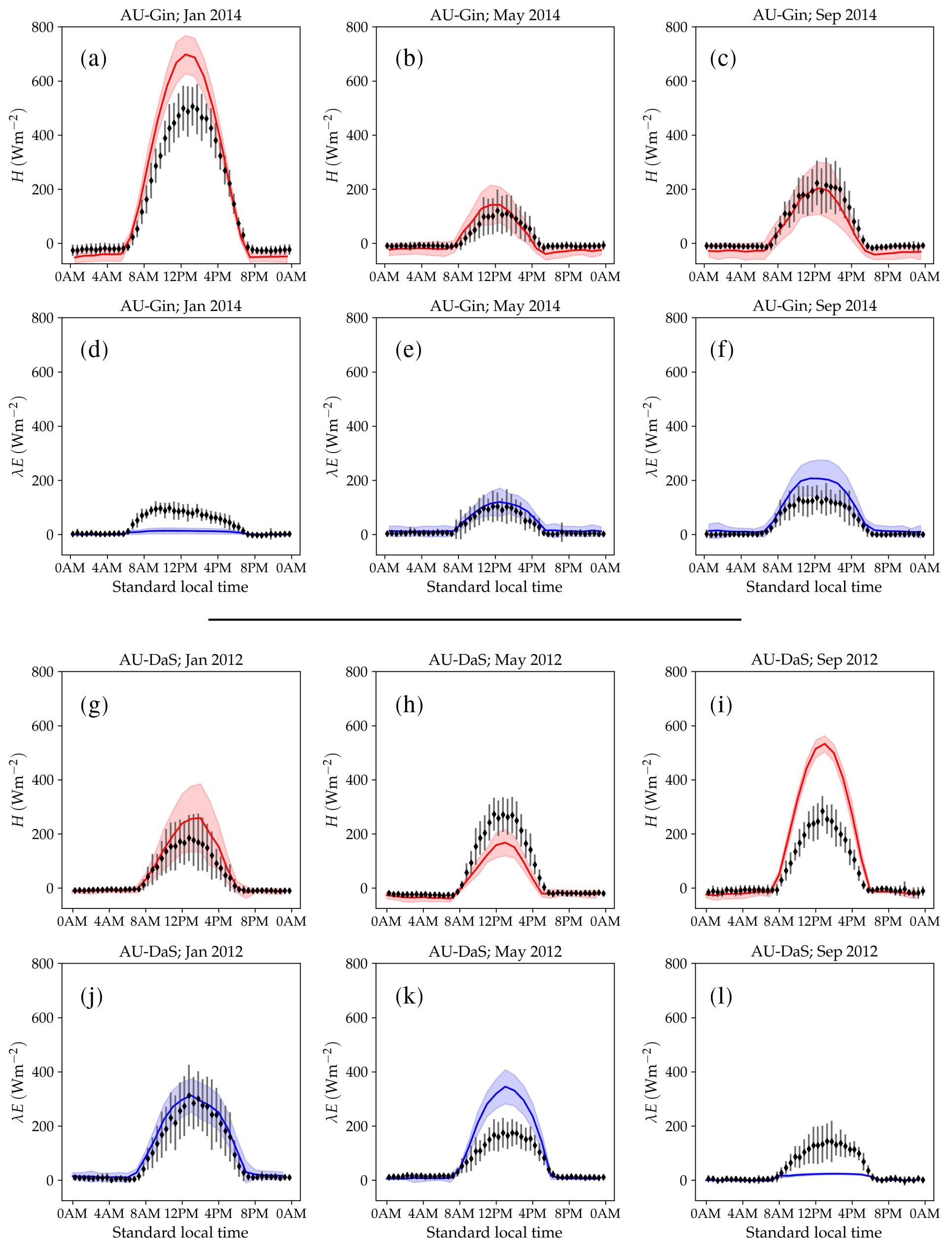
Figure 11Monthly-averaged diurnal cycle of sensible and latent heat flux at the AU-DaP (panels a–f) and AU-DaS (panels g–l) sites in selected months. The red and blue lines represent simulated sensible and latent heat fluxes, respectively. The shaded areas around each curve delimit 1 standard deviation above and below it. The symbols represent monthly-averaged fluxes. The error bars indicate a ±1σ deviation from the observed mean.

Figure 12Monthly-averaged diurnal cycle of sensible and latent heat flux at the BR-Sa1 (panels a–f) and GF-Guy (panels g–l) sites in selected months. The red and blue lines represent simulated sensible and latent heat fluxes, respectively. The shaded areas around each curve delimit 1 standard deviation above and below it. The symbols represent monthly-averaged fluxes. The error bars indicate a ±1σ deviation from the observed mean.
At the AU-Gin site, the shapes of the annual cycles of latent and sensible heat are well-reproduced in the simulations (Fig. 10a). Sensible heat is largest at the beginning of the year, decreases steeply to its minimum around June–July, and starts increasing again around August. The simulation agrees well with measurements most of the year but overestimates sensible heat by ∼45 W m−2 in the first 2 months. Observed latent heat increases at the start of the wet season and dominates the turbulent exchange from May to September. Simulated latent heat is overestimated by up to ∼25 W m−2 in the wet season and underestimated in the dry season. The shift from larger sensible heat to larger latent heat in May is well captured in the simulation, but, due to the overestimation of latent heat, the shift back to larger sensible heat flux is delayed by about 2 months with respect to the observations. The average simulated diurnal cycle of sensible heat is overestimated in January, peaking at ∼700 W m−2 (observed: ∼500 W m−2), while it agrees very well with observations in May and September, both in terms of magnitude and day-to-day variability (Fig. 11a–c).
At the AU-DaS site (Fig. 10b), observed and simulated heat fluxes diverge substantially during the dry season (July–November). Simulated monthly averages of latent heat are ∼20–30 W m−2 above measured values from March to May and ∼30–45 W m−2 below the measurements between August and October. The average simulated latent heat diurnal cycle peaks at ∼350 W m−2 in May (observed: ∼ 175 W m−2) and at ∼ 25 W m−2 in September (observed: ∼ 145 W m−2; Fig. 11j–l). This marked divergence from measured values happens in very dry periods, when the simulated soil moisture in the rooting zone drops close to the wilting point and there is not enough precipitation to replenish it until the start of the wet season. As a consequence, sensible heat is greatly overestimated. Simulated monthly averages rise sharply and peak at ∼ 120–140 W m−2 from September to October, while measured values stay at ∼60 W m−2 throughout the dry season. The average sensible heat diurnal cycle peaks at ∼530 W m−2 in September, while the observed average diurnal peak is slightly under ∼300 W m−2 (Fig. 11g–i).
Monthly averages of sensible and latent heat at the BR-Sa1 tropical rainforest site show little variability throughout the year (Fig. 10c). Measured sensible heat flux stays at ∼20 W m−2 for most of the year and increases to ∼30 W m−2 around August and September, when measured precipitation reaches its minimum. During this period, the soil retains enough moisture in the rooting zone to maintain average latent heat levels at ∼80–90 W m−2. Sensible and latent heat fluxes are systematically overestimated by the model by ∼10–20 W m−2. This overestimation takes place even when simulated net radiation is very close to observations (June to November), so assuming the measurements do not underestimate the fluxes, it must be compensated by an underestimation of ground heat. One possible contributing factor is an underestimation of the heat conductivity, which could be caused by an underestimation of soil moisture in the top soil layer. Unfortunately, soil moisture measurements are not available for this site, so we were not able to test this hypothesis. Average sensible heat flux peaks daily between ∼160 and 275 W m−2 (measured: ∼100–150 W m−2). Latent heat flux peaks daily between ∼280 and 340 W m−2 (measured: ∼220–320 W m−2, Fig. 12a–f).
At the GF-Guy site, another tropical rainforest, monthly averages of sensible heat are overestimated by ∼20 W m−2 throughout the year, while latent heat flux is underestimated by about the same amount. The simulated sensible heat diurnal cycle peaks, on average, by ∼100 W m−2 above the measured values, while the peak of the simulated latent heat diurnal cycle is ∼130 W m−2 below the measured values. There is a marked decrease in simulated latent heat in October and a corresponding sharp increase in sensible heat, due to excessively low soil moisture in the rooting zone in the model. The simulated October average diurnal sensible heat cycle peaks at ∼350 W m−2 (measured: ∼190 W m−2), while the average latent heat diurnal cycle peaks at ∼180 W m−2 (measured: ∼360 W m−2).
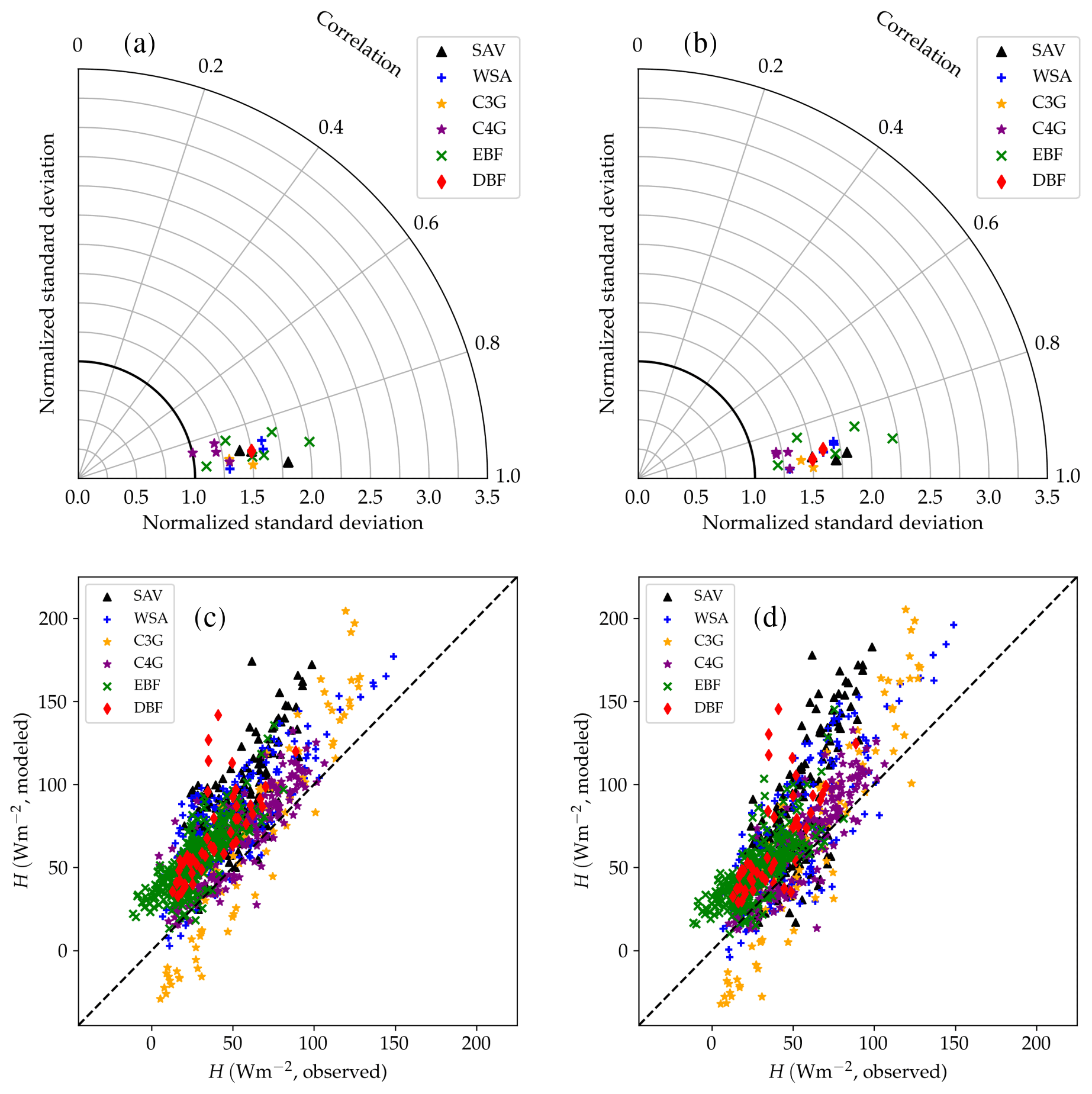
Figure 13Performance of the CLM/BB (a, c) and CLM/Med (b, d) runs for sensible heat flux. The Taylor diagrams (Taylor, 2001) in panels (a) and (b) summarize the degree of agreement between observed and simulated hourly fluxes by relying on the geometrical relationship between the “centred pattern” root mean square difference (defined as ), the correlation coefficient, and the standard deviation of observed and modelled data: . Each point in the polar diagram represents a simulation. The radial coordinate indicates the ratio between modelled and observed standard deviations. The correlation between observed and modelled values is encoded by the polar angle; it decreases anticlockwise from r=1 (perfect correlation) for points situated on the x axis to r=0 for points situated on the y axis. The distance between a point in the diagram and the reference value 1 on the x axis equals the centred pattern RMSE normalized by the standard deviation of the observed values, , and is therefore a measure of the agreement between observed and simulated data. The scatter plots (panels c, d) show a direct comparison of observed and modelled monthly-averaged fluxes. The different symbols refer to different land cover types: savanna (SAV), woody savanna (WSA), C3 grasslands (C3G), C4 grasslands (C4G), evergreen broadleaf forest (EBF), and deciduous broadleaf forest (DBF).
3.4.3 Influence of different stomatal conductance schemes on the simulated heat fluxes
Table 6 and Fig. 13 show model performance statistics for sensible heat fluxes for the CLM/BB and CLM/Med simulations. Correlations between modelled and observed sensible heat fluxes are very high and similar for both runs. For hourly fluxes, r is between ∼0.84 and 96. Correlations between monthly-averaged fluxes are weaker but still high at most sites (r>0.75), but they are very low for SD-Dem, AU-RDF, and ZM-Mon. At these three sites, the CLM/Med simulation shows better correlations and smaller errors than the one using the BB scheme.
Table 6Model performance statistics for simulated hourly (left) and monthly (right) sensible heat fluxes for the CLM/BB and CLM/Med simulations. Bold fonts indicate the model configuration that performed better. The mean and standard deviation of the observed fluxes ( and σo, respectively), shown for reference, are given in W m−2. The RMSE and bias have been normalized by the mean of the observed fluxes for easier cross-site comparison.
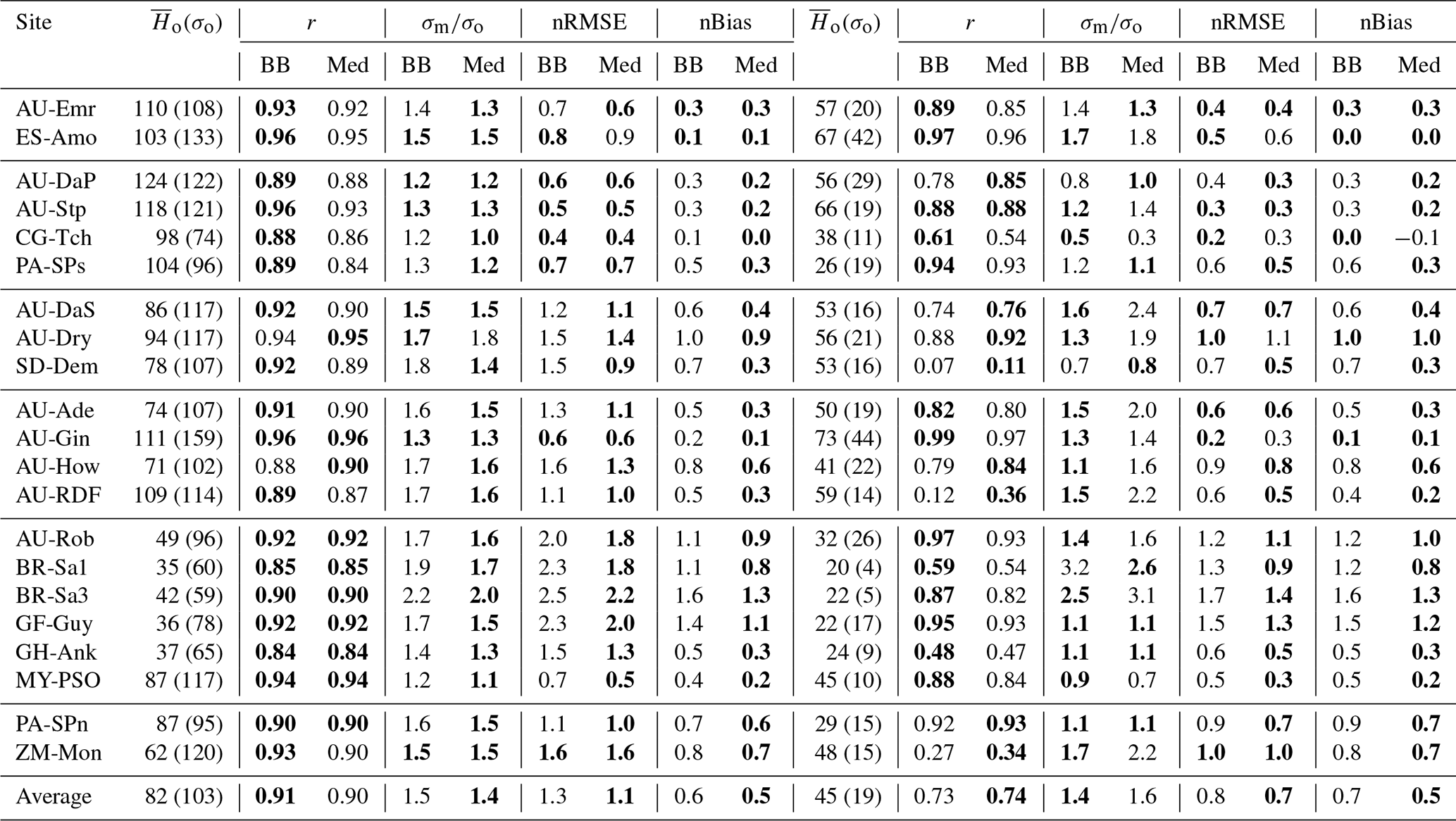
The model tends to overestimate average sensible heat. The hourly and monthly mean biases are non-negative at all sites (except at CG-Tch for monthly fluxes, where it is slightly negative), but normalized RMSE and mean bias are smaller for the CLM/Med run at most sites. The simulations seem to perform comparatively better in grasslands; for the Med simulation, RMSE is between 0.4 and 0.9 of the sample average (hourly fluxes), whereas it is in the 0.6–1.6 range at savanna sites and in the 0.5–2.5 range at forest sites.
The variability of sensible heat flux is also overestimated by the model. In this case, the CLM/Med run performs better than the CLM/BB run for hourly fluxes, but the situation is the reversed for monthly average fluxes. Again, the simulations show better performance at grassland sites; for hourly fluxes, the Med simulation predicts –1.5 in grasslands, ∼1.3–1.8 in savanna and woody savanna sites, and ∼1.1–2.2 in forest sites.
Model performance statistics for latent heat fluxes are presented in Table 7 and Fig. 14. Correlations for hourly fluxes are between 0.7 and 0.9 for most sites. For monthly fluxes, correlations are poorer at forest sites but errors are comparatively small; normalized RMSE is in the 0.1–0.5 range. Hourly correlations are similar for both model configurations at most sites.
Table 7Model performance statistics for simulated hourly (left) and monthly (right) latent heat fluxes for the CLM/BB and CLM/Med simulations. Bold fonts indicate the model configuration that performed better. The mean and standard deviation of the observed fluxes ( and σo, respectively), shown for reference, are given in W m−2. The RMSE and bias have been normalized by the mean of the observed fluxes for easier cross-site comparison.
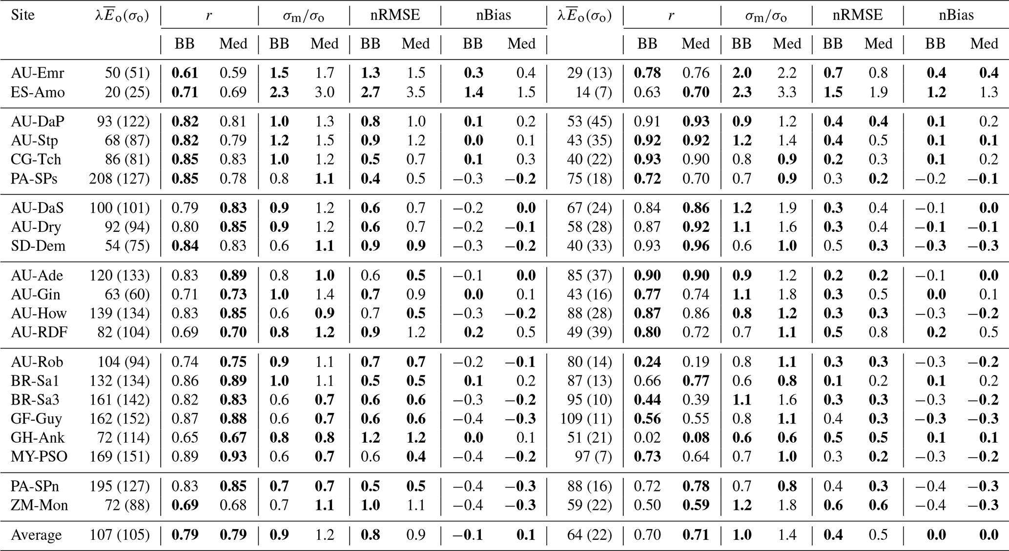
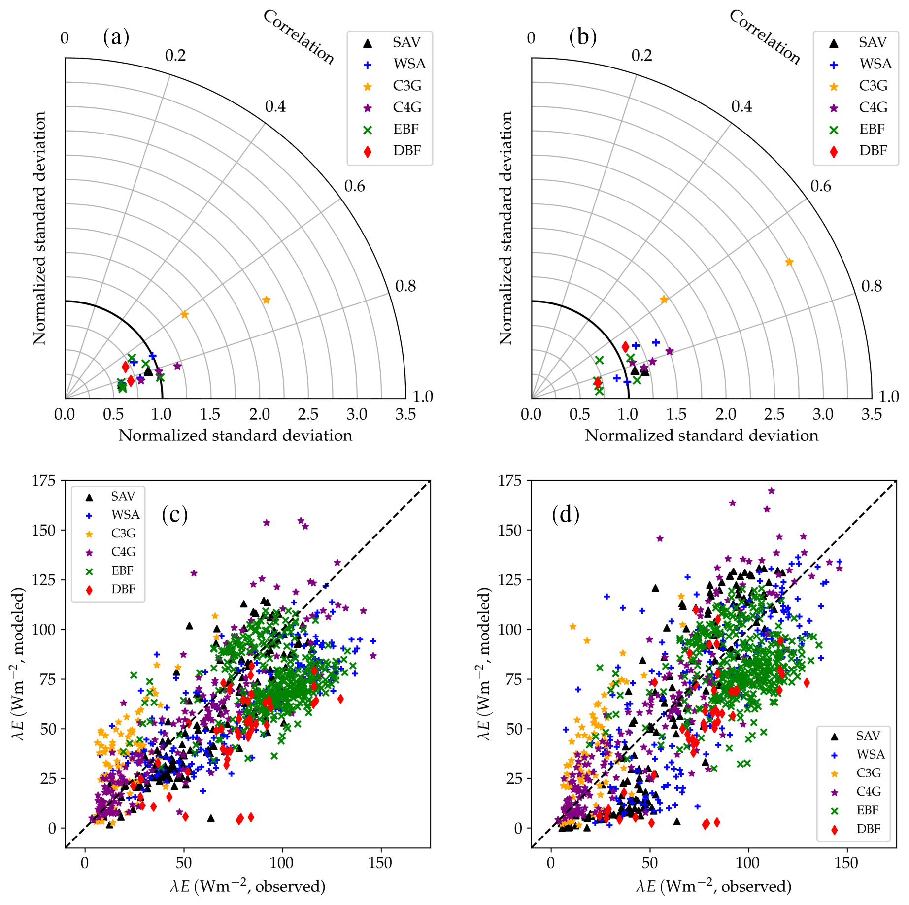
Figure 14Performance of the CLM/BB (a, c) and CLM/Med (b, d) runs for latent heat flux. The Taylor diagram shows statistical metrics calculated from hourly observed and simulated fluxes. The scatter plots show a direct comparison of observed and modelled monthly-averaged fluxes. The different symbols refer to different land cover types: SAV, WSA, C3G, C4G, EBF, and DBF.
Latent heat fluxes tend to be underestimated in forest and savanna sites and overestimated over grasslands. The CLM/BB configuration seems to perform better at grassland sites, while the CLM/Med configuration performs slightly better at forest sites. Results for savanna sites are mixed in terms of RMSE, but the CLM/Med scheme yields somewhat smaller biases.
The variability of simulated latent heat fluxes is larger in the CLM/Med run than in the CLM/BB run. Over C3 grasslands, both LSM runs predict a much larger variability than the observed one. At savanna and woody savanna sites, the CLM/Med run predicts a larger variability than the observed one, both in the hourly and monthly cases, whilst the CLM/BB simulation tends to produce a lower variability. For forest sites, both runs yield σm ≲ σo, with the exception of BR-Sa3 in the CLM/Med run, where the variability of the monthly fluxes is ∼1.6 times larger than the observed one. On average, the CLM/BB simulation shows better agreement with measured variability over grasslands, while CLM/Med performs somewhat better at forest sites.
3.4.4 Alternative model configurations
To evaluate the overall performance of the different model configurations, we considered the cross-site averaged statistics of each simulation (Table 8). Since the covered period differs across sites, this method ensures all sites contribute equally to the result.
Table 8Cross-site averaged model performance statistics for simulated hourly and monthly sensible and latent heat fluxes. RMSE and bias are given in W m−2. Bold fonts indicate the best-performing simulations in each metric.

Figure 15 shows the cross-site averaged metrics on a Taylor diagram. The clumping and clear separation of simulations using different stomatal conductance schemes suggest that this component of the model has a greater influence than the soil water uptake response function on the behaviour of the model, with the possible exception of the linear response function (Noah type), which is much more restrictive than the other three in terms of water uptake. In this case, the variability of modelled latent heat fluxes in the Med simulation is closer to the observed average, lying somewhere between the Med and BB clumps.
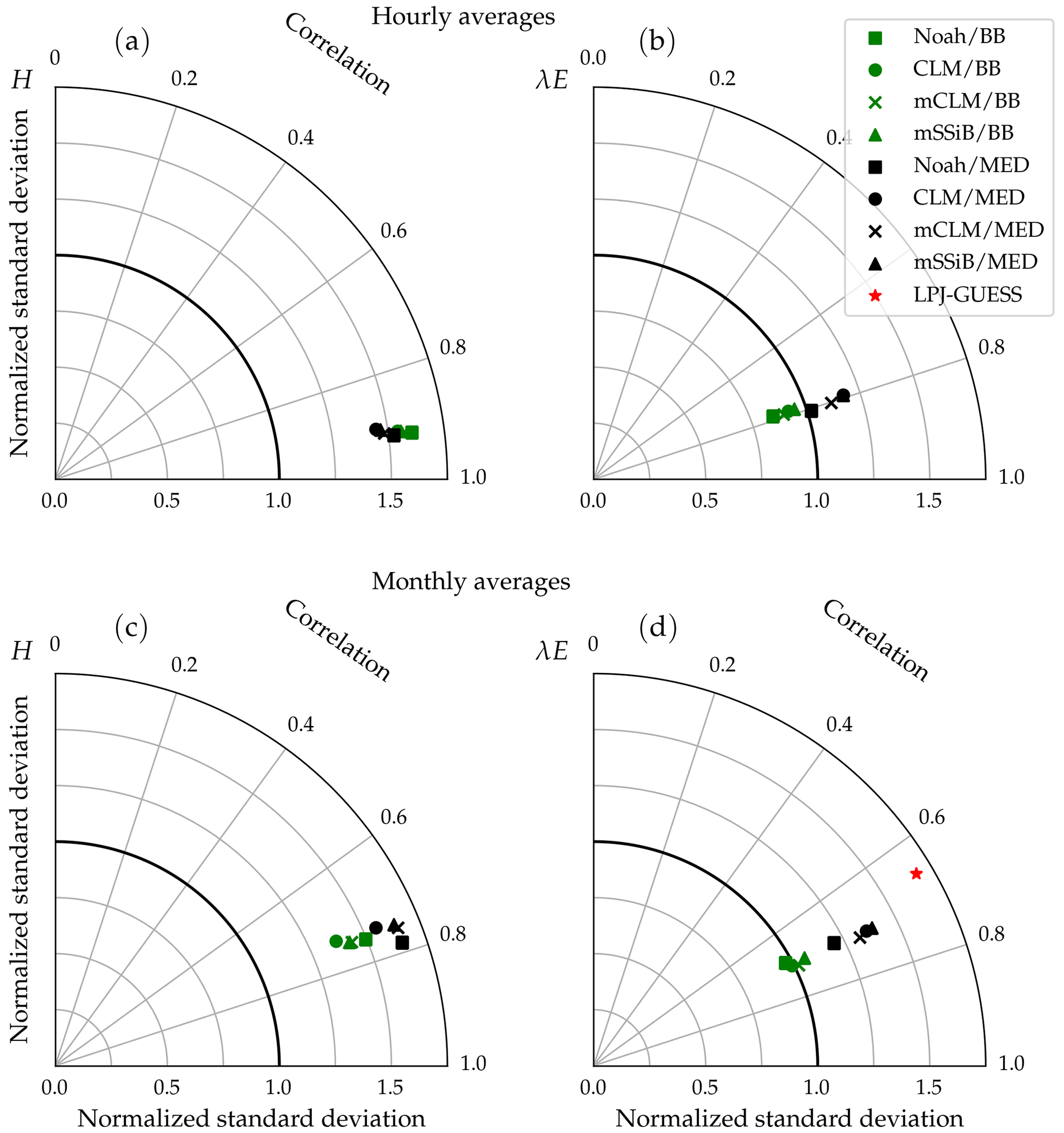
Figure 15Average performance statistics for each model configuration, obtained from modelled and measured hourly (a, b) and monthly (c, d) fluxes of sensible and latent heat flux. The different symbol shapes represent different water uptake response functions (squares: NOAH type; circles: CLM type; crosses: modified CLM type; triangles: SSiB type), and the different colours represent different stomatal conductance schemes (green: Ball–Berry type; black: Medlyn). The red star represents average performance statistics for monthly latent heat fluxes derived from the standard LPJ-GUESS simulation.
Simulated sensible heat fluxes display similar correlation with observations in all runs. The correlation coefficient is very high (r∼0.9) for hourly fluxes and moderately high (r∼0.75) for monthly averages.
Sensible heat is overestimated in all model configurations; the average bias is always positive, but the Med simulations perform better in this respect. In the case of hourly averages, BB runs show an average bias of ∼46 W m−2, while the average value for the Med runs is ∼35 W m−2. Average errors are also smaller in the Med simulations. For hourly fluxes, the average RMSE is ∼90 W m−2 for BB runs and ∼81 W m−2 for Med runs. For monthly fluxes, RMSE averages are ∼31 and ∼28 W m−2, respectively.
The model also generally overestimates the variability of sensible heat. For hourly fluxes, the standard deviation of the sample is, on average, ∼1.6 times greater than the measurements for the BB runs and ∼1.5 for the Med runs. In the case of monthly variability, BB runs perform slightly better; the average standard deviations of modelled fluxes are ∼1.4 and ∼1.6 for the BB and Med runs, respectively.
Correlations between modelled and measured latent heat fluxes are lower than for sensible heat: r∼0.8 for hourly fluxes and ∼0.7 for monthly fluxes. All runs show a similar RMSE: ∼75 and ∼24 W m−2 for hourly and monthly fluxes, respectively. Latent heat is underestimated on average in all configurations. However, the Med runs perform significantly better than the BB runs with this metric. The average bias is W m−2 (BB: W m−2) for hourly fluxes and W m−2 (BB: W m−2) for monthly fluxes. The variability of hourly latent heat fluxes is underestimated in the BB runs by about the same amount that it is overestimated in the Med runs, but in the case of monthly fluxes, BB simulations seem to reproduce the measured variability better (σm∼σo, while σm∼1.3σo for Med runs).
Monthly averages of latent heat simulated by the non-LSM version of LPJ-GUESS show a slightly worse correlation with measurements than the LSM version of the model. The average bias is W m−2, in line with the CLM/Med simulation and significantly lower than the BB simulations, and the RMSE is slightly higher but close to the LSM runs. However, the predicted variability is significantly exaggerated; the standard deviation of the sample of modelled monthly fluxes is, on average, ∼1.7 times larger than observed.
In this work we described a number of modifications to the LPJ-GUESS DGVM aimed at making the model suitable for direct coupling with an atmospheric model. The newly incorporated energy balance module resolves the diurnal cycle of energy and water fluxes between the canopy and the atmosphere, as opposed to LPJ-GUESS's daily calculations. Calculating these fluxes on a sub-daily basis is necessary to match the shorter time step at which atmospheric models operate (typically 1 h or shorter, depending on resolution). The original daily PAR absorption calculations were replaced with a more sophisticated radiative transfer scheme by adapting the models of Sellers (1985) and Dai et al. (2004) to LPJ-GUESS's multi-cohort, multi-layer canopy (some differences in PAR absorption calculated by both schemes are shown in the Supplement). This enables the model to simulate the upwelling short-wave radiation flux on sub-daily timescales. Direct and diffuse radiations are treated separately, which allows us to resolve sunlit and shaded leaves in the canopy. This approach offers a reasonable compromise between accuracy of the modelled fluxes and computational efficiency (Wang and Leuning, 1998). The representation of soil physical processes was modified in two ways. Firstly, the original 1.5 m-deep, two-layer soil column was replaced with a 3 m-deep, nine-layer column. Secondly, the soil heat and water transport schemes were replaced with less parametrized formulations. Soil heat transport is now calculated by solving the heat diffusion equation, while soil water transport is solved by applying Richards' equation. These formulations are better fit to resolve near-surface heat and water fluxes on the sub-daily timescales introduced in the model.
The new physical schemes introduced in this work lead to discrepancies between the LSM and standard LPJ-GUESS, which stem from the different physical environments simulated in the models. Calculating assimilation at the newly simulated canopy temperature, rather than the air temperature, can lead to either higher or lower productivity, depending on the optimal photosynthetic temperature ranges of each PFT and the effect of temperature on N limitation (see Sect. 4.2). Canopy temperature also affects autotrophic respiration, while differences in the simulated soil humidity and temperature impact organic matter decomposition rates and heterotrophic respiration. The combination of these effects results in differences in the simulated equilibrium carbon and nitrogen pools (see the Supplement) and ecosystem–atmosphere carbon fluxes.
4.1 Evaluation of the simulated heat fluxes
The new model was evaluated by comparing simulated fluxes of sensible and latent heat with flux tower measurements at 21 FLUXNET sites. Stöckli et al. (2008) used a similar analysis (including the filtering of fluxes with m s−1) to evaluate the improvement in the performance of CLM 3.5 after introducing nitrogen limitation of photosynthesis, a groundwater model, and an updated formulation of surface resistance. Owing to the different site selection, a rigorous comparison of that study with the results presented in Sect. 3.4.3 is not possible, but average statistics of model performance can provide an overview of how the models compare. Table 9 shows averaged values of the correlation coefficient and RMSE for CLM 3.0, CLM 3.5, and LPJ-GUESS/LSM. Our model seems to yield stronger correlations between measured and observed sensible heat fluxes and RMSE values similar to CLM 3.5, while CLM 3.5 appears to perform better in terms of RMSE for hourly latent heat fluxes, and the correlation between measured and observed monthly latent heat fluxes is stronger. In order to ascertain the significance of these findings, a comparison using the same site-measured fluxes and forcing climate would be needed. Nevertheless, the values presented in Table 9 suggest that the performance of our model is closer to CLM 3.5 than to CLM 3.0.
Table 9Average correlation and RMSE between observed and simulated sensible and latent heat fluxes for LPJ-GUESS/LSM, CLM 3.0, and CLM 3.5. RMSE values (between brackets) are given in W m−2. Hourly and monthly values are labelled (h) and (m), respectively. CLM values correspond to averages over temperate, tropical, and grassland sites as reported in Stöckli et al. (2008). LPJ-GUESS/LSM values correspond to the CLM/Med simulation.
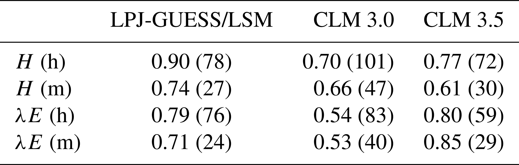
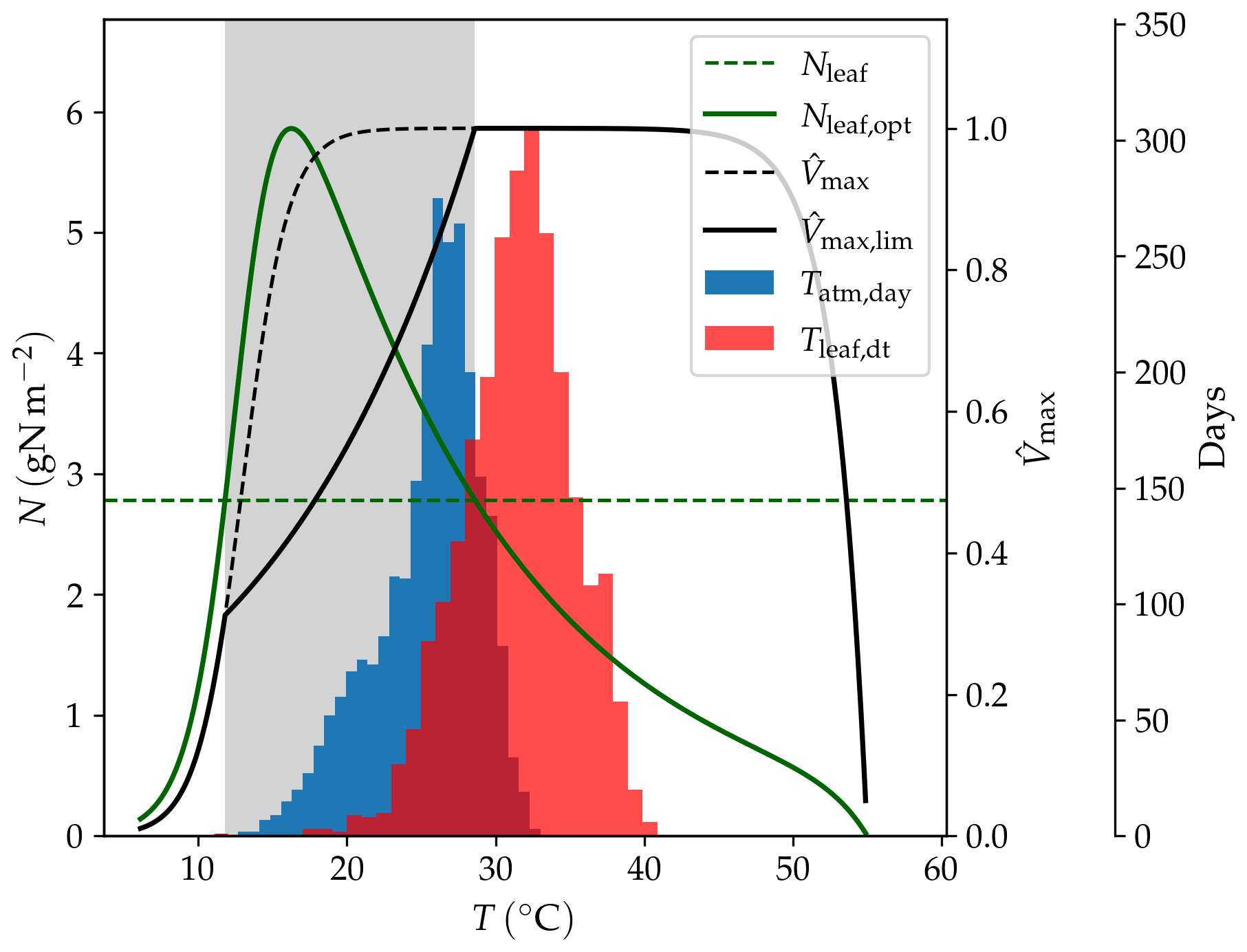
Figure 16Effect of temperature (T) on modelled Vmax; Nleaf,opt: leaf nitrogen content necessary to attain the maximum carboxylation rate; Nleaf: representative leaf nitrogen concentration; : normalized maximum carboxylation rate without nitrogen limitation; : normalized maximum carboxylation rate with nitrogen limitation. The histograms show the frequency of temperatures in the AU-DaP simulation; Tatm,day: daily average of air temperature; Tleaf,dt: daytime average of leaf temperature. The shaded area indicates the temperature range where Vmax is nitrogen-limited.
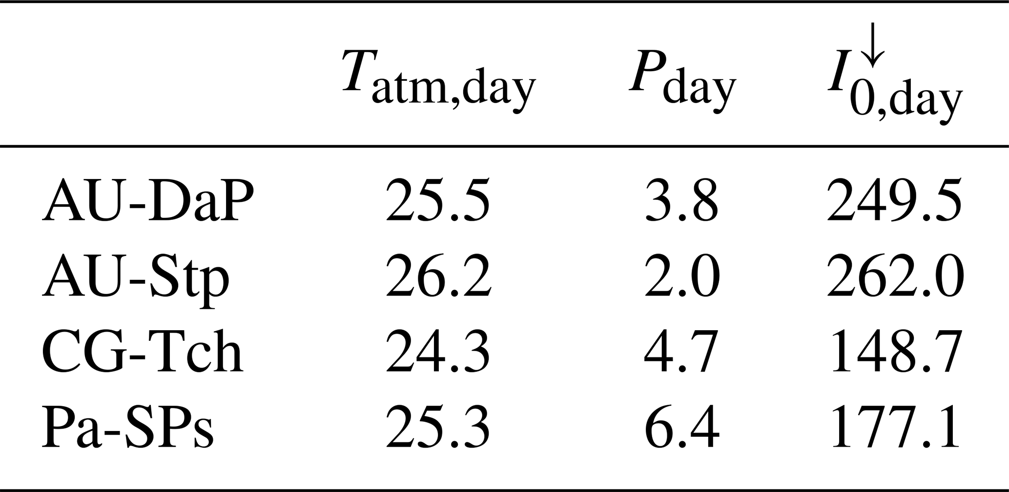
Table 10Daily average climate measured at the four C4 grassland sites in this study. Tatm,day: daily average temperature (∘C); Pday: daily average precipitation (mm d−1); : daily average incoming solar irradiance (W m−2).
Sensible heat is generally overestimated by the LSM. Poor performance in sensible heat flux estimation is a common issue of many land surface models (Best et al., 2015). The reason for this is not well-understood. It has been suggested that the models, the majority of which use similar methods to calculate the turbulent fluxes, do not extract all the information available in the climate forcing data. However, eddy covariance measurements often fail to close the energy balance and might systematically underestimate sensible heat much more than latent heat, which would appear as an overestimation of sensible heat in the simulations. A detailed discussion of these issues is provided in Haughton et al. (2016).
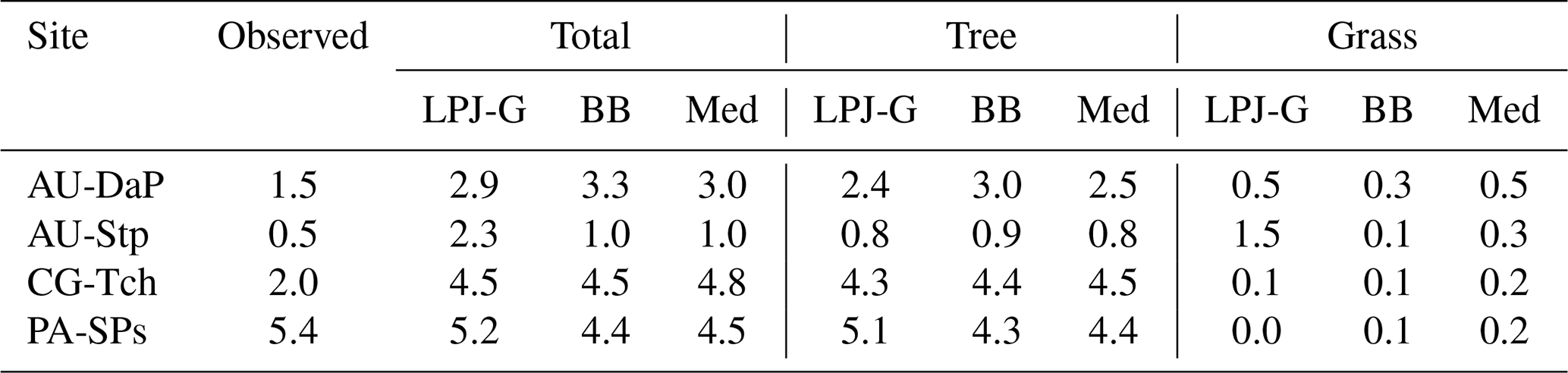
Table 11Observed and simulated LAI at the four C4 grassland sites when all natural PFTs are allowed to grow in the patch. The BB and Med values correspond to LSM simulations using the CLM-type water uptake response function.
One issue in our simulations is the marked underestimation of latent heat flux during extremely dry periods, when the rooting zone is nearly depleted of water available for plant uptake. This, in turn, causes a strong spike in sensible heat (Fig. 10b). All eight model configurations show this behaviour. One possible reason for this is the choice of free drainage boundary conditions at the bottom of the soil column. Simulating groundwater in the model may promote the retention of some soil moisture during dry periods and thus help alleviate this problem (Stöckli et al., 2008). Deeper root profiles and lateral access to soil water may also be important for supporting evapotranspiration in dry periods (Schenk and Jackson, 2002).
We implemented two different stomatal conductance schemes: the Ball–Berry model (Ball et al., 1987) and the Medlyn model (Medlyn et al., 2011). One notable difference between these two models concerns the behaviour of the stomatal conductance when the vapour pressure deficit at the leaf surface (VPD) is small. In the Ball–Berry model, stomatal conductance increases linearly with decreasing VPD, while in the Medlyn model stomatal conductance increases much more rapidly as VPD approaches zero (Fig. 3). Larger stomatal conductance leads to generally higher evapotranspiration values (less negative bias values, Table 8) and enhanced GPP (Fig. 8) in simulations using the Medlyn model. A statistical evaluation of the impact of these differences on the model output was not carried out, but the clumping of symbols representing the two different stomatal conductance models seen in Fig. 15 suggests that the stomatal conductance scheme has a greater impact on the model's behaviour than the choice of soil water uptake response function.
4.2 Why does C4 productivity increase so much in LSM simulations?
The results presented in Sect. 3.4.1 show that predictions of PFT composition, ecosystem productivity, respiration, and carbon dioxide exchange vary between LSM simulations using different water uptake response functions and stomatal conductance schemes and with respect to standard LPJ-GUESS. Very notably, both the gross and net productivities of C4 grasses are substantially enhanced in the LSM simulations compared with the non-LSM model. This results in unrealistically high simulated LAI values at three out of the four sites where the grasses are allowed to grow without competition.
We found that the main reason for this behaviour is the occurrence of higher photosynthetic rates in the LSM simulations due to the mitigation of biochemical N limitation at higher leaf temperatures. Standard LPJ-GUESS uses a daily average of the forcing air temperature as a proxy for leaf temperature in the Vmax calculation. By contrast, LPJ-GUESS/LSM simulates leaf temperature explicitly and uses a daytime average (Eq. 42) to estimate Vmax. This average leaf temperature can be several degrees above the forcing air temperature, which makes it possible to reach the optimal maximum carboxylation rate at lower leaf nitrogen concentrations (see Haxeltine and Prentice, 1996). This makes it easier for the plants to attain the optimal Vmax with the available nitrogen, which enhances productivity. Exceedingly high leaf temperatures can have a negative impact on Vmax due to the thermal breakdown of the biochemical reactions. However, the simulated leaf temperatures are still within the optimal temperature range for C4 grasses (20 to 45 ∘C in LPJ-GUESS). The temperature dependence of Vmax, including the effect on nitrogen limitation, is illustrated in Fig. 16.
At AU-Stp, all three simulations predict much lower productivities. In this case, water availability is the limiting factor. This site receives, on average, considerably less rainwater than the other three C4 grasslands (Table 10), which leads to lower values of the β factor (Eq. 46) and brings photosynthetic rates down.
As pointed out in Sect. 3.2, the simulated PFTs were restricted to grassy types at these sites. Table 11 shows a summary of LAI values predicted by standard LPJ-GUESS and two representative LSM simulations when establishment is not restricted to grassy PFTs. All three experiments predict a mixture of trees and grasses, but total LAI in the LSM runs is much lower than in the simulations where only grasses were allowed to establish. In these runs, competition with trees limits the resources available to grasses, and shading from the taller trees helps lower the average leaf temperature of the grassy understory, all of which helps counteract the effect described above.
4.3 Conclusion and outlook
The developments presented in this paper will enable us to study feedbacks between the climate and the biosphere using the state-of-the-art DGVM LPJ-GUESS directly coupled to an atmospheric model. Work is in progress regarding the development of a flexible interface to enable such coupling and extending the model's ability to simulate cold-climate ecosystems. More work is also needed to characterize and fully understand the model's response to the switch from using air temperature as a proxy for leaf temperature to simulating leaf temperature explicitly, particularly as these concern the productivity of C4 plants in well-watered, no-competition situations (e.g. monoculture crops or managed pastures) and the way the new schemes affect the simulation of the carbon cycle on regional and global scales. These developments will allow us to use LPJ-GUESS/LSM in regional as well as global studies. Given the capacity of LPJ-GUESS to represent land use change and management (Lindeskog et al., 2013, 2021; Olin et al., 2015), the range of applications includes exploring impacts of management on regional climate, which can be an important tool to help devise and assess climate change mitigation policies.
During a given time step Δt, the total amount of water evapotranspired from the sunlit part of the canopy can be expressed as the sum of the contributions from the dry and wet parts:
where Esun is the actual evapotranspiration rate, Esun,tr is the potential rate of transpiration, Esun,ev is the potential rate of evaporation, and Δtwet,sun is the time that the wet part of the sunlit canopy remains wet at the potential evaporation rate. The latter is calculated as
where wc is the current canopy water content (kg m−2).
The evaporation rates in the above equations can be expressed as follows:
where the index i runs over cohorts. Inserting these expressions into Eq. (A1), dividing both sides by Δt, simplifying, and rearranging terms yields
where . Identical equations apply to the shaded part of the canopy.
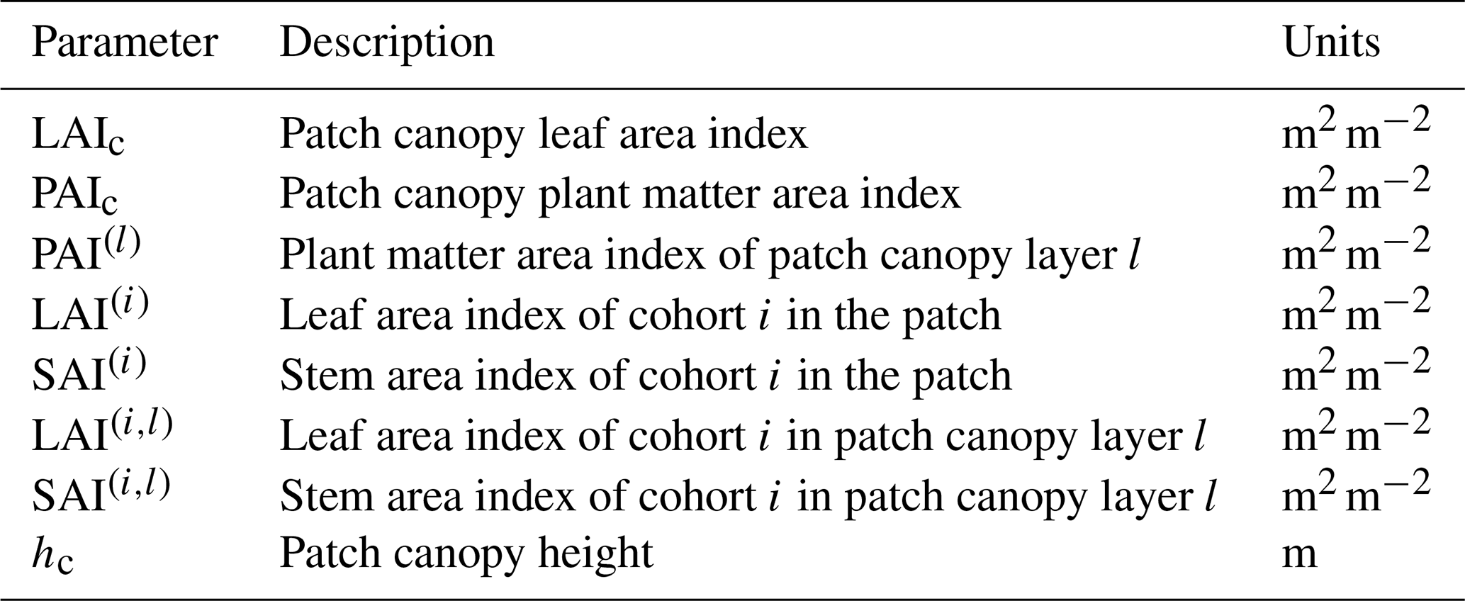
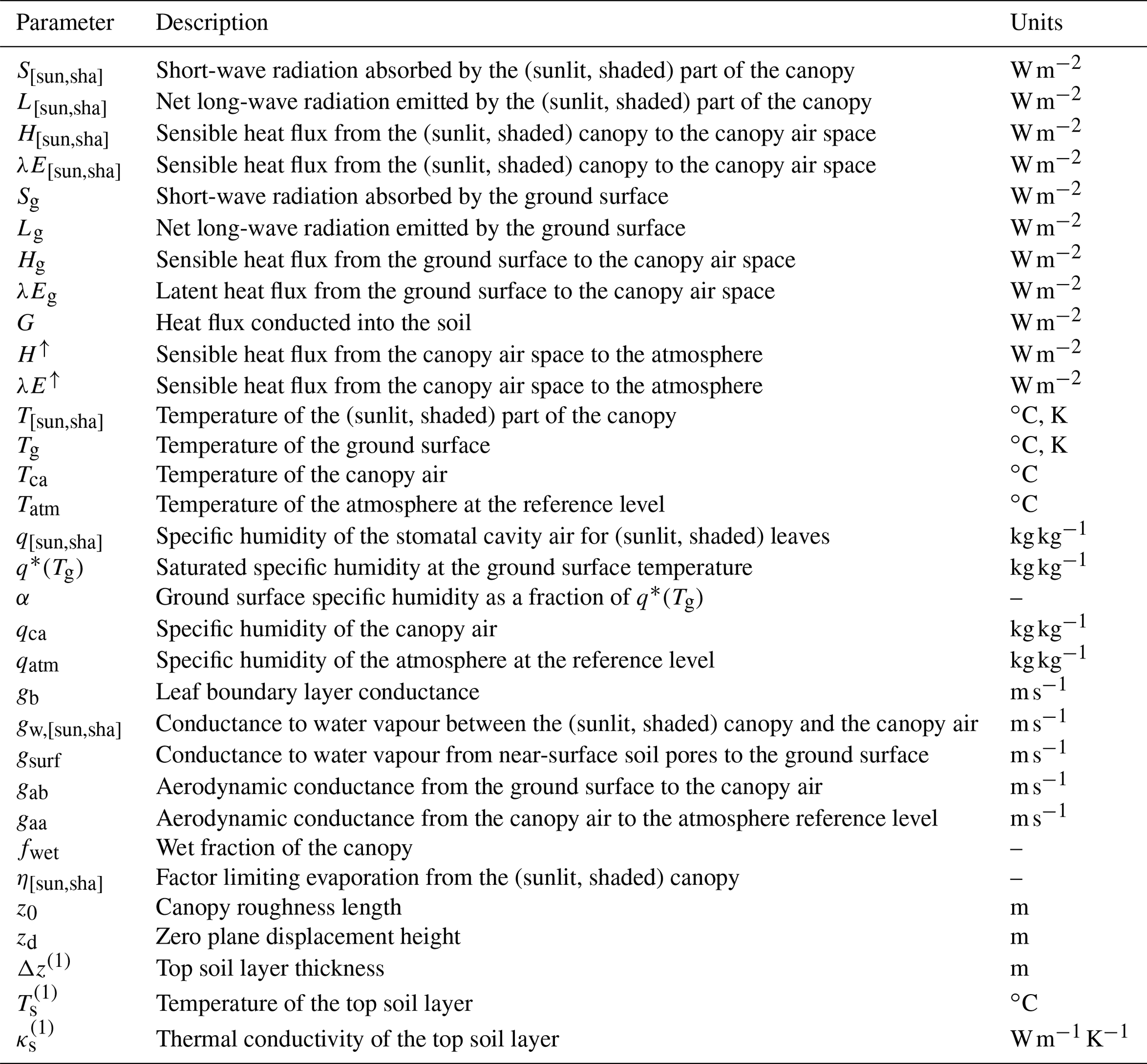
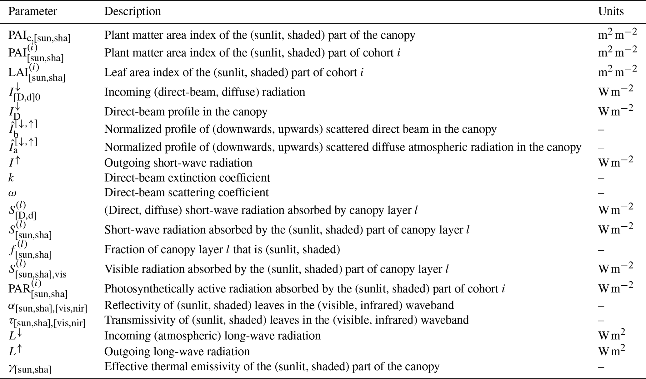

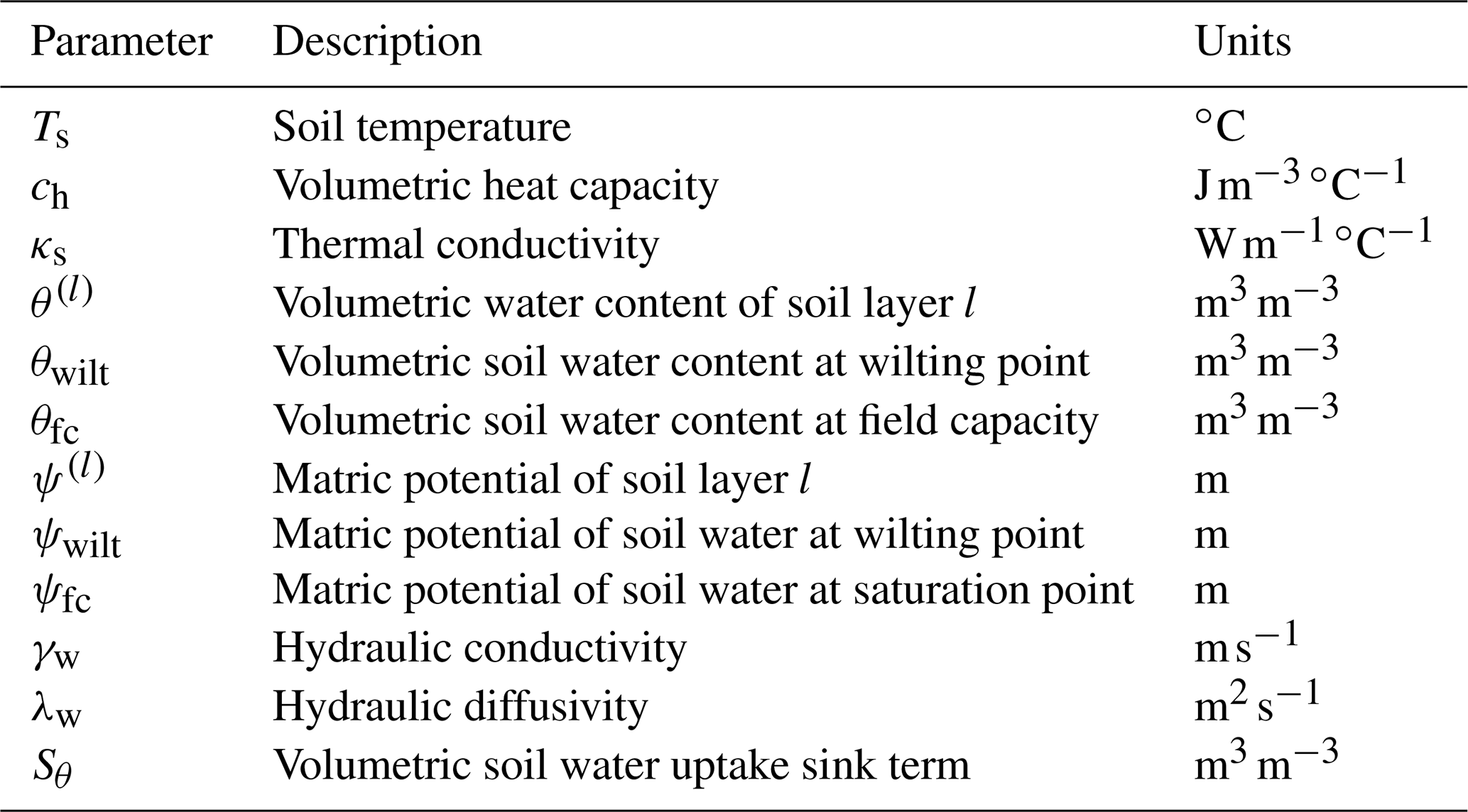
LPJ-GUESS is a worldwide developed and refined DGVM. The model code is managed and maintained by the Department of Physical Geography and Ecosystem Science, Lund University, Sweden. The source code can be made available with a collaboration agreement under the acceptance of certain conditions. For this reason, a DOI for the model code cannot be provided. The code with the augmentations developed for this paper is available to the editor and reviewers via a restricted link, on the condition that the code is used only for review purposes and is deleted after the review process. Additional details and information can be found at the LPJ-GUESS website (http://web.nateko.lu.se/lpj-guess; Smith et al., 2014). The forcing data, evaluation data, model output, and analysis scripts used in this study have been uploaded to a public repository with DOI https://doi.org/10.5281/zenodo.6856036 (Martin-Belda, 2021).
The supplement related to this article is available online at: https://doi.org/10.5194/gmd-15-6709-2022-supplement.
AA had the original idea and motivated the development. DMB designed the model augmentations described in this work with input from all the coauthors. DMB implemented the code, ran the experiments, and performed the model evaluation analysis. All the coauthors provided input regarding the analysis of the results and the discussion and helped shape the final form of the manuscript.
The contact author has declared that none of the authors has any competing interests.
Publisher's note: Copernicus Publications remains neutral with regard to jurisdictional claims in published maps and institutional affiliations.
This research has been supported by the Deutsche Forschungsgemeinschaft (grant no. SCHM 2376/2-1) and the Helmholtz Gemeinschaft (grant no. W3 – Impuls- und Vernetzungsfond). David Wårlind, Stefan Olin, Jing Tang, and Benjamin Smith were financially supported by the strategic research area “Modeling the Regional and Global Earth System” (MERGE). David Wårlind, Stefan Olin, and Benjamin Smith were financially supported by the Swedish national strategic e-science research programme eSSENCE.
The article processing charges for this open-access publication were covered by the Karlsruhe Institute of Technology (KIT).
This paper was edited by David Lawrence and reviewed by two anonymous referees.
Ahlström, A., Smith, B., Lindström, J., Rummukainen, M., and Uvo, C. B.: GCM characteristics explain the majority of uncertainty in projected 21st century terrestrial ecosystem carbon balance, Biogeosciences, 10, 1517–1528, https://doi.org/10.5194/bg-10-1517-2013, 2013. a
Ahlström, A., Schurgers, G., and Smith, B.: The large influence of climate model bias on terrestrial carbon cycle simulations, Environ. Res. Lett., 12, 014004, https://doi.org/10.1088/1748-9326/12/1/014004, 2017. a
Alessandri, A., Catalano, F., De Felice, M., Van Den Hurk, B., Doblas Reyes, F., Boussetta, S., Balsamo, G., and Miller, P. A.: Multi-scale enhancement of climate prediction over land by increasing the model sensitivity to vegetation variability in EC-Earth, Clim. Dynam., 49, 1215–1237, https://doi.org/10.1007/s00382-016-3372-4, 2017. a
Ardö, J., Mölder, M., El-Tahir, B. A., and Elkhidir, H. A. M.: Seasonal variation of carbon fluxes in a sparse savanna in semi arid Sudan, Carbon Balance and Management, 3, 7, https://doi.org/10.1186/1750-0680-3-7, 2008. a
Arneth, A., Harrison, S. P., Zaehle, S., Tsigaridis, K., Menon, S., Bartlein, P. J., Feichter, J., Korhola, A., Kulmala, M., O'Donnell, D., Schurgers, G., Sorvari, S., and Vesala, T.: Terrestrial biogeochemical feedbacks in the climate system, Nat. Geosci., 3, 525–532, https://doi.org/10.1038/ngeo905, 2010. a
Arneth, A., Sitch, S., Pongratz, J., Stocker, B. D., Ciais, P., Poulter, B., Bayer, A. D., Bondeau, A., Calle, L., Chini, L. P., Gasser, T., Fader, M., Friedlingstein, P., Kato, E., Li, W., Lindeskog, M., Nabel, J. E. M. S., Pugh, T. A. M., Robertson, E., Viovy, N., Yue, C., and Zaehle, S.: Historical carbon dioxide emissions caused by land-use changes are possibly larger than assumed, Nat. Geosci., 10, 79–84, https://doi.org/10.1038/ngeo2882, 2017. a
Ball, J. T., Woodrow, I. E., and Berry, J. A.: A Model Predicting Stomatal Conductance and its Contribution to the Control of Photosynthesis under Different Environmental Conditions, in: Progress in Photosynthesis Research, in: Proceedings of the VIIth International Congress on Photosynthesis Providence, Vol. 4, edited by: Biggins, J., Rhode Island, USA, 10–15 August 1986, Springer Netherlands, Dordrecht, 221–224, https://doi.org/10.1007/978-94-017-0519-6_48, 1987. a, b, c
Beringer, J., Hacker, J., Hutley, L. B., Leuning, R., Arndt, S. K., Amiri, R., Bannehr, L., Cernusak, L. A., Grover, S., Hensley, C., Hocking, D., Isaac, P., Jamali, H., Kanniah, K., Livesley, S., Neininger, B., Paw, U., Kyaw, T., Sea, W., Straten, D., Tapper, N., Weinmann, R., Wood, S., and Zegelin, S.: SPECIAL – Savanna Patterns of Energy and Carbon Integrated across the Landscape, B. Am. Meteorol. Soc., 92, 1467–1485, https://doi.org/10.1175/2011BAMS2948.1, 2011. a, b, c, d
Beringer, J., Hutley, L. B., McHugh, I., Arndt, S. K., Campbell, D., Cleugh, H. A., Cleverly, J., Resco de Dios, V., Eamus, D., Evans, B., Ewenz, C., Grace, P., Griebel, A., Haverd, V., Hinko-Najera, N., Huete, A., Isaac, P., Kanniah, K., Leuning, R., Liddell, M. J., Macfarlane, C., Meyer, W., Moore, C., Pendall, E., Phillips, A., Phillips, R. L., Prober, S. M., Restrepo-Coupe, N., Rutledge, S., Schroder, I., Silberstein, R., Southall, P., Yee, M. S., Tapper, N. J., van Gorsel, E., Vote, C., Walker, J., and Wardlaw, T.: An introduction to the Australian and New Zealand flux tower network – OzFlux, Biogeosciences, 13, 5895–5916, https://doi.org/10.5194/bg-13-5895-2016, 2016. a, b
Best, M. J., Abramowitz, G., Johnson, H. R., Pitman, A. J., Balsamo, G., Boone, A., Cuntz, M., Decharme, B., Dirmeyer, P. A., Dong, J., Ek, M., Guo, Z., Haverd, V., van den Hurk, B. J. J., Nearing, G. S., Pak, B., Peters-Lidard, C., Santanello, J. A., Stevens, L., and Vuichard, N.: The Plumbing of Land Surface Models: Benchmarking Model Performance, J. Hydrometeorol., 16, 1425–1442, https://doi.org/10.1175/JHM-D-14-0158.1, 2015. a
Bonal, D., Bosc, A., Ponton, S., Goret, J.-Y., Burban, B., Gross, P., Bonnefond, J.-M., Elbers, J., Longdoz, B., Epron, D., Guehl, J.-M., and Granier, A.: Impact of severe dry season on net ecosystem exchange in the Neotropical rainforest of French Guiana, Global Change Biol., 14, 1917–1933, https://doi.org/10.1111/j.1365-2486.2008.01610.x, 2008. a
Bonan, G.: Ecological Climatology: Concepts and Applications, 3 edn., Cambridge University Press, Cambridge, https://doi.org/10.1017/CBO9781107339200, 2015. a, b, c
Bonan, G.: Climate Change and Terrestrial Ecosystem Modeling, Cambridge University Press, Cambridge, https://doi.org/10.1017/9781107339217, 2019. a
Bonan, G. B., Levis, S., Sitch, S., Vertenstein, M., and Oleson, K. W.: A dynamic global vegetation model for use with climate models: concepts and description of simulated vegetation dynamics, Global Change Biol., 9, 1543–1566, https://doi.org/10.1046/j.1365-2486.2003.00681.x, 2003. a
Bonan, G. B., Williams, M., Fisher, R. A., and Oleson, K. W.: Modeling stomatal conductance in the earth system: linking leaf water-use efficiency and water transport along the soil–plant–atmosphere continuum, Geosci. Model Dev., 7, 2193–2222, https://doi.org/10.5194/gmd-7-2193-2014, 2014. a
Booth, B. B. B., Jones, C. D., Collins, M., Totterdell, I. J., Cox, P. M., Sitch, S., Huntingford, C., Betts, R. A., Harris, G. R., and Lloyd, J.: High sensitivity of future global warming to land carbon cycle processes, Environ. Res. Lett., 7, 024002, https://doi.org/10.1088/1748-9326/7/2/024002, 2012. a
Bristow, M., Hutley, L. B., Beringer, J., Livesley, S. J., Edwards, A. C., and Arndt, S. K.: Quantifying the relative importance of greenhouse gas emissions from current and future savanna land use change across northern Australia, Biogeosciences, 13, 6285–6303, https://doi.org/10.5194/bg-13-6285-2016, 2016. a
Brovkin, V., Sitch, S., Bloh, W. V., Claussen, M., Bauer, E., and Cramer, W.: Role of land cover changes for atmospheric CO2 increase and climate change during the last 150 years, Global Change Biol., 10, 1253–1266, https://doi.org/10.1111/j.1365-2486.2004.00812.x, 2004. a
Christidis, N., Stott, P. A., Hegerl, G. C., and Betts, R. A.: The role of land use change in the recent warming of daily extreme temperatures, Geophys. Res. Lett., 40, 589–594, https://doi.org/10.1002/grl.50159, 2013. a
Ciais, P., Sabine, C., Bala, G., Bopp, L., Brovkin, V., Al, E., and House, J. I.: Carbon and Other Biogeochemical Cycles, Climate Change 2013: The Physical Science Basis. Contribution of Working Group I to the Fifth Assessment Report of the Intergovernmental Panel on Climate Change Change, Cambridge University Press, 465–570, https://doi.org/10.1017/CBO9781107415324.015, 2014. a
Clapp, R. B. and Hornberger, G. M.: Empirical equations for some soil hydraulic properties, Water Resour. Res., 14, 601–604, https://doi.org/10.1029/WR014i004p00601, 1978. a
Clark, M. P., Fan, Y., Lawrence, D. M., Adam, J. C., Bolster, D., Gochis, D. J., Hooper, R. P., Kumar, M., Leung, L. R., Mackay, D. S., Maxwell, R. M., Shen, C., Swenson, S. C., and Zeng, X.: Improving the representation of hydrologic processes in Earth System Models, Water Resour. Res., 51, 5929–5956, https://doi.org/10.1002/2015WR017096, 2015. a
Collatz, G., Ball, J., Grivet, C., and Berry, J. A.: Physiological and environmental regulation of stomatal conductance, photosynthesis and transpiration: a model that includes a laminar boundary layer, Agr. Forest Meteorol., 54, 107–136, https://doi.org/10.1016/0168-1923(91)90002-8, 1991. a
Collatz, G. J., Ribas-Carbo, M., and Berry, J. A.: Coupled Photosynthesis-Stomatal Conductance Model for Leaves of C4 Plants, Funct. Plant Biol., 19, 519–538, https://doi.org/10.1071/pp9920519, 1992. a
Cosby, B. J., Hornberger, G. M., Clapp, R. B., and Ginn, T. R.: A Statistical Exploration of the Relationships of Soil Moisture Characteristics to the Physical Properties of Soils, Water Resour. Res., 20, 682–690, https://doi.org/10.1029/WR020i006p00682, 1984. a
Cramer, W., Bondeau, A., Woodward, F. I., Prentice, I. C., Betts, R. A., Brovkin, V., Cox, P. M., Fisher, V., Foley, J. A., Friend, A. D., Kucharik, C., Lomas, M. R., Ramankutty, N., Sitch, S., Smith, B., White, A., and Young-Molling, C.: Global response of terrestrial ecosystem structure and function to CO2 and climate change: results from six dynamic global vegetation models, Global Change Biol., 7, 357–373, https://doi.org/10.1046/j.1365-2486.2001.00383.x, 2001. a
Dai, Y., Dickinson, R. E., and Wang, Y.-P.: A Two-Big-Leaf Model for Canopy Temperature, Photosynthesis, and Stomatal Conductance, J. Climate, 17, 2281–2299, https://doi.org/10.1175/1520-0442(2004)017<2281:ATMFCT>2.0.CO;2, 2004. a, b, c, d
Damour, G., Simonneau, T., Cochard, H., and Urban, L.: An overview of models of stomatal conductance at the leaf level, Plant Cell Environ., 33, 1419–1438, https://doi.org/10.1111/j.1365-3040.2010.02181.x, 2010. a
De Kauwe, M. G., Medlyn, B. E., Zaehle, S., Walker, A. P., Dietze, M. C., Hickler, T., Jain, A. K., Luo, Y., Parton, W. J., Prentice, I. C., Smith, B., Thornton, P. E., Wang, S., Wang, Y.-P., Wårlind, D., Weng, E., Crous, K. Y., Ellsworth, D. S., Hanson, P. J., Seok Kim, H., Warren, J. M., Oren, R., and Norby, R. J.: Forest water use and water use efficiency at elevated CO2: a model-data intercomparison at two contrasting temperate forest FACE sites, Global Change Biol., 19, 1759–1779, https://doi.org/10.1111/gcb.12164, 2013. a
De Kauwe, M. G., Kala, J., Lin, Y.-S., Pitman, A. J., Medlyn, B. E., Duursma, R. A., Abramowitz, G., Wang, Y.-P., and Miralles, D. G.: A test of an optimal stomatal conductance scheme within the CABLE land surface model, Geosci. Model Dev., 8, 431–452, https://doi.org/10.5194/gmd-8-431-2015, 2015. a
de Noblet-Ducoudré, N., Boisier, J.-P., Pitman, A., Bonan, G. B., Brovkin, V., Cruz, F., Delire, C., Gayler, V., van den Hurk, B. J. J. M., Lawrence, P. J., van der Molen, M. K., Müller, C., Reick, C. H., Strengers, B. J., and Voldoire, A.: Determining Robust Impacts of Land-Use-Induced Land Cover Changes on Surface Climate over North America and Eurasia: Results from the First Set of LUCID Experiments, J. Climate, 25, 3261–3281, https://doi.org/10.1175/JCLI-D-11-00338.1, 2012. a
de Vries, D.: Thermal properties of soils, Physics of Plant Environment, North-Holland Publishing Co., https://doi.org/10.1002/2017RG000581, 1963. a
Dickinson, R. E.: Land Surface Processes and Climate – Surface Albedos and Energy Balance, in: Advances in Geophysics, Theory of Climate, vol. 25, edited by: Saltzman, B., Elsevier, 305–353, https://doi.org/10.1016/S0065-2687(08)60176-4, 1983. a
Döscher, R., Acosta, M., Alessandri, A., Anthoni, P., Arsouze, T., Bergman, T., Bernardello, R., Boussetta, S., Caron, L.-P., Carver, G., Castrillo, M., Catalano, F., Cvijanovic, I., Davini, P., Dekker, E., Doblas-Reyes, F. J., Docquier, D., Echevarria, P., Fladrich, U., Fuentes-Franco, R., Gröger, M., v. Hardenberg, J., Hieronymus, J., Karami, M. P., Keskinen, J.-P., Koenigk, T., Makkonen, R., Massonnet, F., Ménégoz, M., Miller, P. A., Moreno-Chamarro, E., Nieradzik, L., van Noije, T., Nolan, P., O'Donnell, D., Ollinaho, P., van den Oord, G., Ortega, P., Prims, O. T., Ramos, A., Reerink, T., Rousset, C., Ruprich-Robert, Y., Le Sager, P., Schmith, T., Schrödner, R., Serva, F., Sicardi, V., Sloth Madsen, M., Smith, B., Tian, T., Tourigny, E., Uotila, P., Vancoppenolle, M., Wang, S., Wårlind, D., Willén, U., Wyser, K., Yang, S., Yepes-Arbós, X., and Zhang, Q.: The EC-Earth3 Earth system model for the Coupled Model Intercomparison Project 6, Geosci. Model Dev., 15, 2973–3020, https://doi.org/10.5194/gmd-15-2973-2022, 2022. a, b
Egea, G., Verhoef, A., and Vidale, P. L.: Towards an improved and more flexible representation of water stress in coupled photosynthesis–stomatal conductance models, Agr. Forest Meteorol., 151, 1370–1384, https://doi.org/10.1016/j.agrformet.2011.05.019, 2011. a
FAO: The Digitized Soil Map of the World, FAO, Rome, Italy, https://www.fao.org/soils-portal/data-hub/soil-maps-and-databases/faounesco-soil-map-of-the-world/en/ (last access: 22 August 2022), 1991. a
Fisher, R. A., Koven, C. D., Anderegg, W. R. L., Christoffersen, B. O., Dietze, M. C., Farrior, C. E., Holm, J. A., Hurtt, G. C., Knox, R. G., Lawrence, P. J., Lichstein, J. W., Longo, M., Matheny, A. M., Medvigy, D., Muller-Landau, H. C., Powell, T. L., Serbin, S. P., Sato, H., Shuman, J. K., Smith, B., Trugman, A. T., Viskari, T., Verbeeck, H., Weng, E., Xu, C., Xu, X., Zhang, T., and Moorcroft, P. R.: Vegetation demographics in Earth System Models: A review of progress and priorities, Global Change Biol., 24, 35–54, https://doi.org/10.1111/gcb.13910, 2018. a
Forrest, M., Tost, H., Lelieveld, J., and Hickler, T.: Including vegetation dynamics in an atmospheric chemistry-enabled general circulation model: linking LPJ-GUESS (v4.0) with the EMAC modelling system (v2.53), Geosci. Model Dev., 13, 1285–1309, https://doi.org/10.5194/gmd-13-1285-2020, 2020. a, b
Friedlingstein, P., Cox, P., Betts, R., Bopp, L., von Bloh, W., Brovkin, V., Cadule, P., Doney, S., Eby, M., Fung, I., Bala, G., John, J., Jones, C., Joos, F., Kato, T., Kawamiya, M., Knorr, W., Lindsay, K., Matthews, H. D., Raddatz, T., Rayner, P., Reick, C., Roeckner, E., Schnitzler, K.-G., Schnur, R., Strassmann, K., Weaver, A. J., Yoshikawa, C., and Zeng, N.: Climate–Carbon Cycle Feedback Analysis: Results from the C4MIP Model Intercomparison, J. Climate, 19, 3337–3353, https://doi.org/10.1175/JCLI3800.1, 2006. a
Friedlingstein, P., Meinshausen, M., Arora, V. K., Jones, C. D., Anav, A., Liddicoat, S. K., and Knutti, R.: Uncertainties in CMIP5 Climate Projections due to Carbon Cycle Feedbacks, J. Climate, 27, 511–526, https://doi.org/10.1175/JCLI-D-12-00579.1, 2014. a
Friend, A. D., Lucht, W., Rademacher, T. T., Keribin, R., Betts, R., Cadule, P., Ciais, P., Clark, D. B., Dankers, R., Falloon, P. D., Ito, A., Kahana, R., Kleidon, A., Lomas, M. R., Nishina, K., Ostberg, S., Pavlick, R., Peylin, P., Schaphoff, S., Vuichard, N., Warszawski, L., Wiltshire, A., and Woodward, F. I.: Carbon residence time dominates uncertainty in terrestrial vegetation responses to future climate and atmospheric CO2, P. Natl. Acad. Sci. USA, 111, 3280–3285, https://doi.org/10.1073/pnas.1222477110, 2014. a
Gerten, D., Schaphoff, S., Haberlandt, U., Lucht, W., and Sitch, S.: Terrestrial vegetation and water balance – hydrological evaluation of a dynamic global vegetation model, J. Hydrol., 286, 249–270, https://doi.org/10.1016/j.jhydrol.2003.09.029, 2004. a
Green, J. K., Konings, A. G., Alemohammad, S. H., Berry, J., Entekhabi, D., Kolassa, J., Lee, J.-E., and Gentine, P.: Regionally strong feedbacks between the atmosphere and terrestrial biosphere, Nat. Geosci., 10, 410–414, https://doi.org/10.1038/ngeo2957, 2017. a
Green, W. H. and Ampt, G. A.: Studies on Soil Phyics, J. Agr. Sci., 4, 1–24, https://doi.org/10.1017/S0021859600001441, 1911. a
Guo, Z., Dirmeyer, P. A., Koster, R. D., Sud, Y. C., Bonan, G., Oleson, K. W., Chan, E., Verseghy, D., Cox, P., Gordon, C. T., McGregor, J. L., Kanae, S., Kowalczyk, E., Lawrence, D., Liu, P., Mocko, D., Lu, C.-H., Mitchell, K., Malyshev, S., McAvaney, B., Oki, T., Yamada, T., Pitman, A., Taylor, C. M., Vasic, R., and Xue, Y.: GLACE: The Global Land–Atmosphere Coupling Experiment. Part II: Analysis, J. Hydrometeorol., 7, 611–625, https://doi.org/10.1175/JHM511.1, 2006. a
Haughton, N., Abramowitz, G., Pitman, A. J., Or, D., Best, M. J., Johnson, H. R., Balsamo, G., Boone, A., Cuntz, M., Decharme, B., Dirmeyer, P. A., Dong, J., Ek, M., Guo, Z., Haverd, V., van den Hurk, B. J. J., Nearing, G. S., Pak, B., Santanello, J. A., Stevens, L. E., and Vuichard, N.: The Plumbing of Land Surface Models: Is Poor Performance a Result of Methodology or Data Quality?, J. Hydrometeorol., 17, 1705–1723, https://doi.org/10.1175/JHM-D-15-0171.1, 2016. a
Haxeltine, A. and Prentice, I. C.: A General Model for the Light-Use Efficiency of Primary Production, Funct. Ecol., 10, 551–561, https://doi.org/10.2307/2390165, 1996. a, b, c, d
Huntingford, C., Lowe, J. A., Booth, B. B. B., Jones, C. D., Harris, G. R., Gohar, L. K., and Meir, P.: Contributions of carbon cycle uncertainty to future climate projection spread, Tellus B, 61, 355–360, https://doi.org/10.1111/j.1600-0889.2009.0, 2009. a
Hutley, L. B., Beringer, J., Isaac, P. R., Hacker, J. M., and Cernusak, L. A.: A sub-continental scale living laboratory: Spatial patterns of savanna vegetation over a rainfall gradient in northern Australia, Agr. Forest Meteorol., 151, 1417–1428, https://doi.org/10.1016/j.agrformet.2011.03.002, 2011. a, b
Irving, L. J. and Robinson, D.: A dynamic model of Rubisco turnover in cereal leaves, New Phytol., 169, 493–504, https://doi.org/10.1111/j.1469-8137.2005.01584.x, 2006. a
Johansen, O.: Thermal Conductivity of Soils, Tech. rep., Cold Regions Research and Engineering Lab Hanover NH, https://apps.dtic.mil/sti/citations/ADA044002 (last access: 22 August 2022), 1977. a
Jones, C., Robertson, E., Arora, V., Friedlingstein, P., Shevliakova, E., Bopp, L., Brovkin, V., Hajima, T., Kato, E., Kawamiya, M., Liddicoat, S., Lindsay, K., Reick, C. H., Roelandt, C., Segschneider, J., and Tjiputra, J.: Twenty-First-Century Compatible CO2 Emissions and Airborne Fraction Simulated by CMIP5 Earth System Models under Four Representative Concentration Pathways, J. Climate, 26, 4398–4413, https://doi.org/10.1175/JCLI-D-12-00554.1, 2013. a
Kosugi, Y., Takanashi, S., Ohkubo, S., Matsuo, N., Tani, M., Mitani, T., Tsutsumi, D., and Nik, A. R.: CO2 exchange of a tropical rainforest at Pasoh in Peninsular Malaysia, Agr. Forest Meteorol., 148, 439–452, https://doi.org/10.1016/j.agrformet.2007.10.007, 2008. a
Krinner, G., Viovy, N., de Noblet-Ducoudré, N., Ogée, J., Polcher, J., Friedlingstein, P., Ciais, P., Sitch, S., and Prentice, I. C.: A dynamic global vegetation model for studies of the coupled atmosphere-biosphere system, Global Biogeochem. Cy., 19, GB1015, https://doi.org/10.1029/2003GB002199, 2005. a
Kucharik, C. J., Norman, J. M., and Gower, S. T.: Measurements of branch area and adjusting leaf area index indirect measurements, Agr. Forest Meteorol., 91, 69–88, https://doi.org/10.1016/S0168-1923(98)00064-1, 1998. a
Kumar, S., Dirmeyer, P. A., Merwade, V., DelSole, T., Adams, J. M., and Niyogi, D.: Land use/cover change impacts in CMIP5 climate simulations: A new methodology and 21st century challenges, J. Geophys. Res.-Atmos., 118, 6337–6353, https://doi.org/10.1002/jgrd.50463, 2013. a
Kurz, W. A., Dymond, C. C., Stinson, G., Rampley, G. J., Neilson, E. T., Carroll, A. L., Ebata, T., and Safranyik, L.: Mountain pine beetle and forest carbon feedback to climate change, Nature, 452, 987–990, https://doi.org/10.1038/nature06777, 2008. a
Lamarque, J.-F., Dentener, F., McConnell, J., Ro, C.-U., Shaw, M., Vet, R., Bergmann, D., Cameron-Smith, P., Dalsoren, S., Doherty, R., Faluvegi, G., Ghan, S. J., Josse, B., Lee, Y. H., MacKenzie, I. A., Plummer, D., Shindell, D. T., Skeie, R. B., Stevenson, D. S., Strode, S., Zeng, G., Curran, M., Dahl-Jensen, D., Das, S., Fritzsche, D., and Nolan, M.: Multi-model mean nitrogen and sulfur deposition from the Atmospheric Chemistry and Climate Model Intercomparison Project (ACCMIP): evaluation of historical and projected future changes, Atmos. Chem. Phys., 13, 7997–8018, https://doi.org/10.5194/acp-13-7997-2013, 2013. a, b
Lambers, H., Chapin, F. S., and Pons, T. L.: Plant Physiological Ecology, Springer, New York, NY, https://doi.org/10.1007/978-0-387-78341-3, 2008. a
Lawrence, D. and Vandecar, K.: Effects of tropical deforestation on climate and agriculture, Nat. Clim. Change, 5, 27–36, https://doi.org/10.1038/nclimate2430, 2015. a
Lawrence, D. M., Oleson, K. W., Flanner, M. G., Thornton, P. E., Swenson, S. C., Lawrence, P. J., Zeng, X., Yang, Z.-L., Levis, S., Sakaguchi, K., Bonan, G. B., and Slater, A. G.: Parameterization improvements and functional and structural advances in Version 4 of the Community Land Model, J. Adv. Model. Earth Sy., 3, M03001, https://doi.org/10.1029/2011MS00045, 2011. a
Lawrence, P. J. and Chase, T. N.: Representing a new MODIS consistent land surface in the Community Land Model (CLM 3.0), J. Geophys. Res.-Biogeo., 112, G01023, https://doi.org/10.1029/2006JG000168, 2007. a
Le Quéré, C., Andrew, R. M., Friedlingstein, P., Sitch, S., Hauck, J., Pongratz, J., Pickers, P. A., Korsbakken, J. I., Peters, G. P., Canadell, J. G., Arneth, A., Arora, V. K., Barbero, L., Bastos, A., Bopp, L., Chevallier, F., Chini, L. P., Ciais, P., Doney, S. C., Gkritzalis, T., Goll, D. S., Harris, I., Haverd, V., Hoffman, F. M., Hoppema, M., Houghton, R. A., Hurtt, G., Ilyina, T., Jain, A. K., Johannessen, T., Jones, C. D., Kato, E., Keeling, R. F., Goldewijk, K. K., Landschützer, P., Lefèvre, N., Lienert, S., Liu, Z., Lombardozzi, D., Metzl, N., Munro, D. R., Nabel, J. E. M. S., Nakaoka, S., Neill, C., Olsen, A., Ono, T., Patra, P., Peregon, A., Peters, W., Peylin, P., Pfeil, B., Pierrot, D., Poulter, B., Rehder, G., Resplandy, L., Robertson, E., Rocher, M., Rödenbeck, C., Schuster, U., Schwinger, J., Séférian, R., Skjelvan, I., Steinhoff, T., Sutton, A., Tans, P. P., Tian, H., Tilbrook, B., Tubiello, F. N., van der Laan-Luijkx, I. T., van der Werf, G. R., Viovy, N., Walker, A. P., Wiltshire, A. J., Wright, R., Zaehle, S., and Zheng, B.: Global Carbon Budget 2018, Earth Syst. Sci. Data, 10, 2141–2194, https://doi.org/10.5194/essd-10-2141-2018, 2018. a
Levis, S., Foley, J. A., and Pollard, D.: Large-Scale Vegetation Feedbacks on a Doubled CO2 Climate, J. Climate, 13, 1313–1325, https://doi.org/10.1175/1520-0442(2000)013<1313:LSVFOA>2.0.CO;2, 2000. a
Lindeskog, M., Arneth, A., Bondeau, A., Waha, K., Seaquist, J., Olin, S., and Smith, B.: Implications of accounting for land use in simulations of ecosystem carbon cycling in Africa, Earth Syst. Dynam., 4, 385–407, https://doi.org/10.5194/esd-4-385-2013, 2013. a, b
Lindeskog, M., Smith, B., Lagergren, F., Sycheva, E., Ficko, A., Pretzsch, H., and Rammig, A.: Accounting for forest management in the estimation of forest carbon balance using the dynamic vegetation model LPJ-GUESS (v4.0, r9710): implementation and evaluation of simulations for Europe, Geosci. Model Dev., 14, 6071–6112, https://doi.org/10.5194/gmd-14-6071-2021, 2021. a, b
López-Ballesteros, A., Serrano-Ortiz, P., Kowalski, A. S., Sánchez-Cañete, E. P., Scott, R. L., and Domingo, F.: Subterranean ventilation of allochthonous CO2 governs net CO2 exchange in a semiarid Mediterranean grassland, Agr. Forest Meteorol., 234-235, 115–126, https://doi.org/10.1016/j.agrformet.2016.12.021, 2017. a, b
Lorenz, R., Davin, E. L., Lawrence, D. M., Stöckli, R., and Seneviratne, S. I.: How Important is Vegetation Phenology for European Climate and Heat Waves?, J. Climate, 26, 10077–10100, https://doi.org/10.1175/JCLI-D-13-00040.1, 2013. a
Luo, Y.: Terrestrial Carbon–Cycle Feedback to Climate Warming, Annu. Rev. Ecol. Evol. S., 38, 683–712, https://doi.org/10.1146/annurev.ecolsys.38.091206.095808, 2007. a
Martin-Belda, D.: Forcing data, evaluation data, model output and analysis scripts used in LPJ-GUESS/LSM description paper [Data set], Zenodo [data set], https://doi.org/10.5281/zenodo.6856036, 2021. a
McGuire, A. D., Sitch, S., Clein, J. S., Dargaville, R., Esser, G., Foley, J., Heimann, M., Joos, F., Kaplan, J., Kicklighter, D. W., Meier, R. A., Melillo, J. M., Moore III, B., Prentice, I. C., Ramankutty, N., Reichenau, T., Schloss, A., Tian, H., Williams, L. J., and Wittenberg, U.: Carbon balance of the terrestrial biosphere in the Twentieth Century: Analyses of CO2, climate and land use effects with four process-based ecosystem models, Global Biogeochem. Cy., 15, 183–206, https://doi.org/10.1029/2000GB001298, 2001. a
Medlyn, B. E., Duursma, R. A., Eamus, D., Ellsworth, D. S., Prentice, I. C., Barton, C. V. M., Crous, K. Y., Angelis, P. D., Freeman, M., and Wingate, L.: Reconciling the optimal and empirical approaches to modelling stomatal conductance, Global Change Biol., 17, 2134–2144, https://doi.org/10.1111/j.1365-2486.2010.02375.x, 2011. a, b, c
Medvigy, D., Walko, R. L., Otte, M. J., and Avissar, R.: Simulated Changes in Northwest U.S. Climate in Response to Amazon Deforestation, J. Climate, 26, 9115–9136, https://doi.org/10.1175/JCLI-D-12-00775.1, 2013. a
Merbold, L., Ardö, J., Arneth, A., Scholes, R. J., Nouvellon, Y., de Grandcourt, A., Archibald, S., Bonnefond, J. M., Boulain, N., Brueggemann, N., Bruemmer, C., Cappelaere, B., Ceschia, E., El-Khidir, H. A. M., El-Tahir, B. A., Falk, U., Lloyd, J., Kergoat, L., Le Dantec, V., Mougin, E., Muchinda, M., Mukelabai, M. M., Ramier, D., Roupsard, O., Timouk, F., Veenendaal, E. M., and Kutsch, W. L.: Precipitation as driver of carbon fluxes in 11 African ecosystems, Biogeosciences, 6, 1027–1041, https://doi.org/10.5194/bg-6-1027-2009, 2009. a, b, c
Metsaranta, J. M., Kurz, W. A., Neilson, E. T., and Stinson, G.: Implications of future disturbance regimes on the carbon balance of Canada's managed forest (2010–2100), Tellus B, 62, 719–728, https://doi.org/10.1111/j.1600-0889.2010.00487.x, 2010. a
Monsi, M. and Saeki, T.: On the Factor Light in Plant Communities and its Importance for Matter Production, Jpn. J. Bot., 14, 22–52, 1953. a, b
Monsi, M. and Saeki, T.: On the Factor Light in Plant Communities and its Importance for Matter Production, Ann. Bot.-London, 95, 549–567, https://doi.org/10.1093/aob/mci052, 2005. a, b
Narisma, G. T. and Pitman, A. J.: The Impact of 200 Years of Land Cover Change on the Australian Near-Surface Climate, J. Hydrometeorol., 4, 424–436, https://doi.org/10.1175/1525-7541(2003)4<424:TIOYOL>2.0.CO;2, 2003. a
Niu, G.-Y., Yang, Z.-L., Mitchell, K. E., Chen, F., Ek, M. B., Barlage, M., Kumar, A., Manning, K., Niyogi, D., Rosero, E., Tewari, M., and Xia, Y.: The community Noah land surface model with multiparameterization options (Noah-MP): 1. Model description and evaluation with local-scale measurements, J. Geophys. Res., 116, D12109, https://doi.org/10.1029/2010JD015139, 2011. a
O'ishi, R. and Abe-Ouchi, A.: Influence of dynamic vegetation on climate change arising from increasing CO2, Clim. Dynam., 33, 645–663, https://doi.org/10.1007/s00382-009-0611-y, 2009. a
Oleson, K. W., Lawrence, D. M., Flanner, M. G., Kluzek, E., Levis, S., Swenson, S. C., Thornton, E., Dai, A., Decker, M., Dickinson, R., Feddema, J., Heald, C. L., Lamarque, J.-F., Niu, G.-Y., Qian, T., Running, S., Sakaguchi, K., Slater, A., Stöckli, R., Wang, A., Yang, L., Zeng, X., and Zeng, X.: Technical Description of version 4.0 of the Community Land Model (CLM), OPENSKY, https://doi.org/10.5065/D6FB50WZ, 2010. a, b, c
Olin, S., Lindeskog, M., Pugh, T. A. M., Schurgers, G., Wårlind, D., Mishurov, M., Zaehle, S., Stocker, B. D., Smith, B., and Arneth, A.: Soil carbon management in large-scale Earth system modelling: implications for crop yields and nitrogen leaching, Earth Syst. Dynam., 6, 745–768, https://doi.org/10.5194/esd-6-745-2015, 2015. a, b
Pastorello, G., Trotta, C., Canfora, E., Chu, H., Christianson, D., Cheah, Y.-W., Poindexter, C., Chen, J., Elbashandy, A., Humphrey, M., Isaac, P., Polidori, D., Reichstein, M., Ribeca, A., van Ingen, C., Vuichard, N., Zhang, L., Amiro, B., Ammann, C., Arain, M. A., Ardö, J., Arkebauer, T., Arndt, S. K., Arriga, N., Aubinet, M., Aurela, M., Baldocchi, D., Barr, A., Beamesderfer, E., Marchesini, L. B., Bergeron, O., Beringer, J., Bernhofer, C., Berveiller, D., Billesbach, D., Black, T. A., Blanken, P. D., Bohrer, G., Boike, J., Bolstad, P. V., Bonal, D., Bonnefond, J.-M., Bowling, D. R., Bracho, R., Brodeur, J., Brümmer, C., Buchmann, N., Burban, B., Burns, S. P., Buysse, P., Cale, P., Cavagna, M., Cellier, P., Chen, S., Chini, I., Christensen, T. R., Cleverly, J., Collalti, A., Consalvo, C., Cook, B. D., Cook, D., Coursolle, C., Cremonese, E., Curtis, P. S., D'Andrea, E., da Rocha, H., Dai, X., Davis, K. J., Cinti, B. D., de Grandcourt, A., Ligne, A. D., De Oliveira, R. C., Delpierre, N., Desai, A. R., Di Bella, C. M., di Tommasi, P., Dolman, H., Domingo, F., Dong, G., Dore, S., Duce, P., Dufrêne, E., Dunn, A., Dušek, J., Eamus, D., Eichelmann, U., ElKhidir, H. A. M., Eugster, W., Ewenz, C. M., Ewers, B., Famulari, D., Fares, S., Feigenwinter, I., Feitz, A., Fensholt, R., Filippa, G., Fischer, M., Frank, J., Galvagno, M., Gharun, M., Gianelle, D., Gielen, B., Gioli, B., Gitelson, A., Goded, I., Goeckede, M., Goldstein, A. H., Gough, C. M., Goulden, M. L., Graf, A., Griebel, A., Gruening, C., Grünwald, T., Hammerle, A., Han, S., Han, X., Hansen, B. U., Hanson, C., Hatakka, J., He, Y., Hehn, M., Heinesch, B., Hinko-Najera, N., Hörtnagl, L., Hutley, L., Ibrom, A., Ikawa, H., Jackowicz-Korczynski, M., Janouš, D., Jans, W., Jassal, R., Jiang, S., Kato, T., Khomik, M., Klatt, J., Knohl, A., Knox, S., Kobayashi, H., Koerber, G., Kolle, O., Kosugi, Y., Kotani, A., Kowalski, A., Kruijt, B., Kurbatova, J., Kutsch, W. L., Kwon, H., Launiainen, S., Laurila, T., Law, B., Leuning, R., Li, Y., Liddell, M., Limousin, J.-M., Lion, M., Liska, A. J., Lohila, A., López-Ballesteros, A., López-Blanco, E., Loubet, B., Loustau, D., Lucas-Moffat, A., Lüers, J., Ma, S., Macfarlane, C., Magliulo, V., Maier, R., Mammarella, I., Manca, G., Marcolla, B., Margolis, H. A., Marras, S., Massman, W., Mastepanov, M., Matamala, R., Matthes, J. H., Mazzenga, F., McCaughey, H., McHugh, I., McMillan, A. M. S., Merbold, L., Meyer, W., Meyers, T., Miller, S. D., Minerbi, S., Moderow, U., Monson, R. K., Montagnani, L., Moore, C. E., Moors, E., Moreaux, V., Moureaux, C., Munger, J. W., Nakai, T., Neirynck, J., Nesic, Z., Nicolini, G., Noormets, A., Northwood, M., Nosetto, M., Nouvellon, Y., Novick, K., Oechel, W., Olesen, J. E., Ourcival, J.-M., Papuga, S. A., Parmentier, F.-J., Paul-Limoges, E., Pavelka, M., Peichl, M., Pendall, E., Phillips, R. P., Pilegaard, K., Pirk, N., Posse, G., Powell, T., Prasse, H., Prober, S. M., Rambal, S., Rannik, Ü., Raz-Yaseef, N., Rebmann, C., Reed, D., Resco de Dios, V., Restrepo-Coupe, N., Reverter, B. R., Roland, M., Sabbatini, S., Sachs, T., Saleska, S. R., Sánchez-Cañete, E. P., Sanchez-Mejia, Z. M., Schmid, H. P., Schmidt, M., Schneider, K., Schrader, F., Schroder, I., Scott, R. L., Sedlák, P., Serrano-Ortíz, P., Shao, C., Shi, P., Shironya, I., Siebicke, L., Šigut, L., Silberstein, R., Sirca, C., Spano, D., Steinbrecher, R., Stevens, R. M., Sturtevant, C., Suyker, A., Tagesson, T., Takanashi, S., Tang, Y., Tapper, N., Thom, J., Tomassucci, M., Tuovinen, J.-P., Urbanski, S., Valentini, R., van der Molen, M., van Gorsel, E., van Huissteden, K., Varlagin, A., Verfaillie, J., Vesala, T., Vincke, C., Vitale, D., Vygodskaya, N., Walker, J. P., Walter-Shea, E., Wang, H., Weber, R., Westermann, S., Wille, C., Wofsy, S., Wohlfahrt, G., Wolf, S., Woodgate, W., Li, Y., Zampedri, R., Zhang, J., Zhou, G., Zona, D., Agarwal, D., Biraud, S., Torn, M., and Papale, D.: The FLUXNET2015 dataset and the ONEFlux processing pipeline for eddy covariance data, Sci. Data, 7, 225, https://doi.org/10.1038/s41597-020-0534-3, 2020. a
Peñuelas, J., Rutishauser, T., and Filella, I.: Phenology Feedbacks on Climate Change, Science, 324, 887–888, https://doi.org/10.1126/science.1173004, 2009. a
Philip, J. R.: Evaporation, and moisture and heat fields in the soil, J. Meteorol., 14, 354–366, https://doi.org/10.1175/1520-0469(1957)014<0354:EAMAHF>2.0.CO;2, 1957. a
Piao, S., Sitch, S., Ciais, P., Friedlingstein, P., Peylin, P., Wang, X., Ahlström, A., Anav, A., Canadell, J. G., Cong, N., Huntingford, C., Jung, M., Levis, S., Levy, P. E., Li, J., Lin, X., Lomas, M. R., Lu, M., Luo, Y., Ma, Y., Myneni, R. B., Poulter, B., Sun, Z., Wang, T., Viovy, N., Zaehle, S., and Zeng, N.: Evaluation of terrestrial carbon cycle models for their response to climate variability and to CO2 trends, Global Change Biol., 19, 2117–2132, https://doi.org/10.1111/gcb.12187, 2013. a
Pitman, A. J.: The evolution of, and revolution in, land surface schemes designed for climate models, Int. J. Climatol., 23, 479–510, https://doi.org/10.1002/joc.893, 2003. a
Pongratz, J., Reick, C. H., Raddatz, T., and Claussen, M.: Biogeophysical versus biogeochemical climate response to historical anthropogenic land cover change, Geophys. Res. Lett., 37, L08702, https://doi.org/10.1029/2010GL043010, 2010. a
Prentice, I. C., Cramer, W., Harrison, S. P., Leemans, R., Monserud, R. A., and Solomon, A. M.: Special Paper: A Global Biome Model Based on Plant Physiology and Dominance, Soil Properties and Climate, J. Biogeogr., 19, 117–134, https://doi.org/10.2307/2845499, 1992. a
Press, W. H. (Ed.): Numerical recipes in Fortran 77: the art of scientific computing, 2nd edn. reprinted with corrections, in: Numerical recipes in FORTRAN, vol. [1,1], Cambridge Univ. Press, Cambridge, oCLC 249641445, 2003. a, b
Quillet, A., Peng, C., and Garneau, M.: Toward dynamic global vegetation models for simulating vegetation–climate interactions and feedbacks: recent developments, limitations, and future challenges, Environ. Rev., 18, 333–353, https://doi.org/10.1139/A10-016, 2010. a
Raupach, M. R.: Simplified expressions for vegetation roughness length and zero-plane displacement as functions of canopy height and area index, Bound.-Lay. Meteorol., 71, 211–216, https://doi.org/10.1007/BF00709229, 1994. a
Raupach, M. R.: Corrigenda, Bound.-Lay. Meteorol., 76, 303–304, https://doi.org/10.1007/BF00709356, 1995. a
Reich, P. B., Walters, M. B., and Ellsworth, D. S.: Leaf age and season influence the relationships between leaf nitrogen, leaf mass per area and photosynthesis in maple and oak trees, Plant Cell Environ., 14, 251–259, https://doi.org/10.1111/j.1365-3040.1991.tb01499.x, 1991. a
Richards, L. A.: Capillary conduction of liquids through porous mediums, Physics, 1, 318–333, https://doi.org/10.1063/1.1745010, 1931. a
Sakaguchi, K. and Zeng, X.: Effects of soil wetness, plant litter, and under-canopy atmospheric stability on ground evaporation in the Community Land Model (CLM3.5), J. Geophys. Res.-Atmos., 114, D01107, https://doi.org/10.1029/2008JD010834, 2009. a, b
Saleska, S. R., Miller, S. D., Matross, D. M., Goulden, M. L., Wofsy, S. C., da Rocha, H. R., de Camargo, P. B., Crill, P., Daube, B. C., de Freitas, H. C., Hutyra, L., Keller, M., Kirchhoff, V., Menton, M., Munger, J. W., Pyle, E. H., Rice, A. H., and Silva, H.: Carbon in Amazon Forests: Unexpected Seasonal Fluxes and Disturbance-Induced Losses, Science, 302, 1554–1557, https://doi.org/10.1126/science.1091165, 2003. a, b
Schenk, H. J. and Jackson, R. B.: Rooting depths, lateral root spreads and below-ground/above-ground allometries of plants in water-limited ecosystems, J. Ecol., 90, 480–494, https://doi.org/10.1046/j.1365-2745.2002.00682.x, 2002. a
Schroder, I., Kuske, T., and Zegelin, S.: Eddy Covariance Dataset for Arcturus (2011–2013), Geoscience Australia, Tech. rep., Canberra, https://doi.org/102.100.100/14249, 2014. a, b
Schurgers, G., Ahlström, A., Arneth, A., Pugh, T. A. M., and Smith, B.: Climate Sensitivity Controls Uncertainty in Future Terrestrial Carbon Sink, Geophys. Res. Lett., 45, 4329–4336, https://doi.org/10.1029/2018GL077528, 2018. a
Sellers, P., Randall, D., Collatz, G., Berry, J., Field, C., Dazlich, D., Zhang, C., Collelo, G., and Bounoua, L.: A Revised Land Surface Parameterization (SiB2) for Atmospheric GCMS. Part I: Model Formulation, J. Climate, 9, 676–705, https://doi.org/10.1175/1520-0442(1996)009<0676:ARLSPF>2.0.CO;2, 1996. a
Sellers, P. J.: Canopy reflectance, photosynthesis and transpiration, Int. J. Remote Sens., 6, 1335–1372, https://doi.org/10.1080/01431168508948283, 1985. a
Sitch, S., Smith, B., Prentice, I. C., Arneth, A., Bondeau, A., Cramer, W., Kaplan, J. O., Levis, S., Lucht, W., Sykes, M. T., Thonicke, K., and Venevsky, S.: Evaluation of ecosystem dynamics, plant geography and terrestrial carbon cycling in the LPJ dynamic global vegetation model, Global Change Biol., 9, 161–185, https://doi.org/10.1046/j.1365-2486.2003.00569.x, 2003. a, b
Smith, B., Prentice, I. C., and Sykes, M. T.: Representation of vegetation dynamics in the modelling of terrestrial ecosystems: comparing two contrasting approaches within European climate space, Global Ecol., 10, 621–637, https://doi.org/10.1046/j.1466-822X.2001.t01-1-00256.x, 2001. a, b, c, d
Smith, B., Samuelsson, P., Wramneby, A., and Rummukainen, M.: A model of the coupled dynamics of climate, vegetation and terrestrial ecosystem biogeochemistry for regional applications, Tellus A, 63, 87–106, https://doi.org/10.1111/j.1600-0870.2010.00477.x, 2011. a, b
Smith, B., Wårlind, D., Arneth, A., Hickler, T., Leadley, P., Siltberg, J., and Zaehle, S.: Implications of incorporating N cycling and N limitations on primary production in an individual-based dynamic vegetation model, Biogeosciences, 11, 2027–2054, https://doi.org/10.5194/bg-11-2027-2014, 2014. a, b, c, d, e, f
Stefani, P., Belelli Marchesini, L., Consalvo, C., Forgione, A., Bombelli, A., Grieco, E., Mazzenga, F., Vittorini, E., Papale, D., and Valentini, R.: Eddy Flux Tower in Ankasa Park: a new facility for the study of the carbon cycle of primary tropical forests in Africa, EGU General Assembly Conference Abstracts, 11, 9538, http://adsabs.harvard.edu/abs/2009EGUGA..11.9538S (last access: 22 August 2022), 2009. a
Stöckli, R., Lawrence, D. M., Niu, G.-Y., Oleson, K. W., Thornton, P. E., Yang, Z.-L., Bonan, G. B., Denning, A. S., and Running, S. W.: Use of FLUXNET in the Community Land Model development, J. Geophys. Res.-Biogeo., 113, G01025, https://doi.org/10.1029/2007JG000562, 2008. a, b, c, d
Swann, A. L. S., Fung, I. Y., and Chiang, J. C. H.: Mid-latitude afforestation shifts general circulation and tropical precipitation, P. Natl. Acad. Sci. USA, 109, 712–716, https://doi.org/10.1073/pnas.1116706108, 2012. a
Taylor, K. E.: Summarizing multiple aspects of model performance in a single diagram, J. Geophys. Res.-Atmos., 106, 7183–7192, https://doi.org/10.1029/2000JD900719, 2001. a
Thonicke, K., Venevsky, S., Sitch, S., and Cramer, W.: The role of fire disturbance for global vegetation dynamics: coupling fire into a Dynamic Global Vegetation Model, Global Ecol. Biogeogr., 10, 661–677, https://doi.org/10.1046/j.1466-822X.2001.00175.x, 2001. a
Wang, Y. P. and Leuning, R.: A two-leaf model for canopy conductance, photosynthesis and partitioning of available energy I: Model description and comparison with a multi-layered model, Agr. Forest Meteorol., 91, 89–111, https://doi.org/10.1016/S0168-1923(98)00061-6, 1998. a
Wania, R., Ross, I., and Prentice, I. C.: Integrating peatlands and permafrost into a dynamic global vegetation model: 1. Evaluation and sensitivity of physical land surface processes: Peatlands and Permafrost in LPJ, 1, Global Biogeochem. Cy., 23, https://doi.org/10.1029/2008GB003412, 2009. a
Weiss, M., Miller, P. A., van den Hurk, B. J. J. M., van Noije, T., Ştefănescu, S., Haarsma, R., van Ulft, L. H., Hazeleger, W., Le Sager, P., Smith, B., and Schurgers, G.: Contribution of Dynamic Vegetation Phenology to Decadal Climate Predictability, J. Climate, 27, 8563–8577, https://doi.org/10.1175/JCLI-D-13-00684.1, 2014. a
Werth, D. and Avissar, R.: The local and global effects of Amazon deforestation, J. Geophys. Res.-Atmos., 107, LBA 55-1–LBA 55-8, https://doi.org/10.1029/2001JD000717, 2002. a
Wolf, A., Ciais, P., Bellassen, V., Delbart, N., Field, C. B., and Berry, J. A.: Forest biomass allometry in global land surface models, Global Biogeochem. Cy., 25, GB3015, https://doi.org/10.1029/2010GB003917, 2011. a
Wolf, S., Eugster, W., Potvin, C., Turner, B. L., and Buchmann, N.: Carbon sequestration potential of tropical pasture compared with afforestation in Panama, Global Change Biol., 17, 2763–2780, https://doi.org/10.1111/j.1365-2486.2011.02460.x, 2011. a, b
Wramneby, A., Smith, B., and Samuelsson, P.: Hot spots of vegetation-climate feedbacks under future greenhouse forcing in Europe, J. Geophys. Res.-Atmos., 115, D21119, https://doi.org/10.1029/2010JD014307, 2010. a, b
Wu, M., Schurgers, G., Rummukainen, M., Smith, B., Samuelsson, P., Jansson, C., Siltberg, J., and May, W.: Vegetation–climate feedbacks modulate rainfall patterns in Africa under future climate change, Earth Syst. Dynam., 7, 627–647, https://doi.org/10.5194/esd-7-627-2016, 2016. a
Wu, M., Schurgers, G., Ahlström, A., Rummukainen, M., Miller, P. A., Smith, B., and May, W.: Impacts of land use on climate and ecosystem productivity over the Amazon and the South American continent, Environ. Res. Lett., 12, 054016, https://doi.org/10.1088/1748-9326/aa6fd6, 2017. a
Wu, M., Smith, B., Schurgers, G., Ahlström, A., and Rummukainen, M.: Vegetation-Climate Feedbacks Enhance Spatial Heterogeneity of Pan-Amazonian Ecosystem States Under Climate Change, Geophys. Res. Lett., 48, e2020GL092001, https://doi.org/10.1029/2020GL092001, 2021. a, b
Xue, Y., Sellers, P. J., Kinter, J. L., and Shukla, J.: A Simplified Biosphere Model for Global Climate Studies, J. Climate, 4, 345–364, https://doi.org/10.1175/1520-0442(1991)004<0345:ASBMFG>2.0.CO;2, 1991. a
Zeng, N., Neelin, J. D., Lau, K.-M., and Tucker, C. J.: Enhancement of Interdecadal Climate Variability in the Sahel by Vegetation Interaction, Science, 286, 1537–1540, https://doi.org/10.1126/science.286.5444.1537, 1999. a
Zhang, W., Jansson, C., Miller, P. A., Smith, B., and Samuelsson, P.: Biogeophysical feedbacks enhance the Arctic terrestrial carbon sink in regional Earth system dynamics, Biogeosciences, 11, 5503–5519, https://doi.org/10.5194/bg-11-5503-2014, 2014. a
Zhang, W., Miller, P. A., Jansson, C., Samuelsson, P., Mao, J., and Smith, B.: Self-Amplifying Feedbacks Accelerate Greening and Warming of the Arctic, Geophys. Res. Lett., 45, 7102–7111, https://doi.org/10.1029/2018GL077830, 2018. a
Zobler, L.: A world soil file grobal climate modeling, NASA Tech. Memo, 32, https://cir.nii.ac.jp/crid/1570009749339537280 (last access: 22 August 2022), 1986. a
Zscheischler, J., Mahecha, M. D., von Buttlar, J., Harmeling, S., Jung, M., Rammig, A., Randerson, J. T., Schölkopf, B., Seneviratne, S. I., Tomelleri, E., Zaehle, S., and Reichstein, M.: A few extreme events dominate global interannual variability in gross primary production, Environ. Res. Lett., 9, 035001, https://doi.org/10.1088/1748-9326/9/3/035001, 2014. a
- Abstract
- Introduction
- Model description
- Model verification and evaluation
- Discussion and summary
- Appendix A: Derivation of the canopy conductance for water vapour flux
- Appendix B: List of symbols, parameters, and variables used in the model description
- Code and data availability
- Author contributions
- Competing interests
- Disclaimer
- Financial support
- Review statement
- References
- Supplement