the Creative Commons Attribution 4.0 License.
the Creative Commons Attribution 4.0 License.
 | 26 Jan 2022
Numerically consistent budgets of potential temperature, momentum, and moisture in Cartesian coordinates: application to the WRF model
Matthias Göbel
Stefano Serafin
Mathias W. Rotach
Numerically accurate budgeting of the forcing terms in the governing equations of a numerical weather prediction model is hard to achieve. Because individual budget terms are generally 2 to 3 orders of magnitude larger than the resulting tendency, exact closure of the budget can only be achieved if the contributing terms are calculated consistently with the model numerics.
We present WRFlux, an open-source software that allows precise budget evaluation for the WRF model and, in comparison to existing similar tools, incorporates new capabilities. WRFlux transforms the budget equations from the terrain-following grid of the model to the Cartesian coordinate system, permitting a simplified interpretation of budgets obtained from simulations over non-uniform orography. WRFlux also decomposes the resolved advection into mean advective and resolved turbulence components, which is useful in the analysis of large-eddy simulation output. The theoretical framework of the numerically consistent coordinate transformation is also applicable to other models. We demonstrate the performance and a possible application of WRFlux with an idealized simulation of convective boundary layer growth over a mountain range. We illustrate the effect of inconsistent approximations by comparing the results of WRFlux with budget calculations using a lower-order advection operator and two alternative formulations of the coordinate transformation. With WRFlux, the sum of all forcing terms for potential temperature, water vapor mixing ratio, and momentum agrees with the respective model tendencies to high precision. In contrast, the approximations lead to large residuals: the root mean square error between the sum of the diagnosed forcing terms and the actual tendency is 1 to 3 orders of magnitude larger than with WRFlux.
- Article
(1759 KB) - Full-text XML
- BibTeX
- EndNote


Budget analysis for variables of a numerical weather prediction model is a widely used tool when examining physical processes in the atmospheric sciences. Energy and mass budgeting has been used, for instance, to understand the governing dynamics of thermally driven circulations in the mountain boundary layer (Rampanelli et al., 2004; Lehner and Whiteman, 2014; Potter et al., 2018). Other examples, such as Lilly and Jewett (1990), Kiranmayi and Maloney (2011), and Huang et al. (2018) are listed in Chen et al. (2020). In a budget analysis, the relative weight and the spatial or temporal patterns of individual forcing terms are assessed. For potential temperature, for instance, forcing terms include resolved advection, subgrid-scale diffusion, and diabatic processes, such as radiative heating and latent heat release.
Large competing forcing terms adding up to a relatively small total tendency make the budget calculation particularly error-prone (Chen et al., 2020): if approximations inconsistent with the model numerics are made, the sum of all forcing terms can result in an unclosed budget with a large residual, even if the relative error of each forcing term is small.
For the WRF model (Skamarock and Klemp, 2008), there have been several attempts to achieve precise budget calculations, e.g., Lehner (2012), Moisseeva and Steyn (2014), Potter et al. (2018), and Chen et al. (2020). Chen et al. (2020) developed a momentum and potential temperature budget analysis tool for the WRF model. Their study focuses on the horizontal momentum budget in idealized 2D simulations of slantwise convection and squall lines and demonstrates that very small residual values can be achieved by retrieving all relevant forcing terms during the runtime of the model. Chen et al. (2020) compare their results with other ways of approximating the momentum budget: neglection of grid staggering, use of a lower-order advection operator, and use of the advective form instead of the flux form of the equations. The authors demonstrate that these approximations strongly deteriorate the budget closure.
Even if the equations in the numerical model are cast in flux form, some authors use the advective form in budget analyses as they find it easier to interpret (e.g., Umek et al., 2021). Although it is possible to discretize an advective-form equation in a way that it is numerically equivalent to the respective flux form (Xue and Lin, 2001), the advective form may hinder interpretation (Lee et al., 2004): if the fluxes on two opposing sides of a grid box are equal, the tendency component is zero for the flux form but not necessarily for the advective form of the equations.
By design, the budget computation method of Chen et al. (2020) cannot discriminate between tendencies caused by resolved-scale and subgrid-scale turbulence. This is important, especially when doing large-eddy simulations, which partially resolve the turbulence spectrum. A budget analysis tool capable of estimating tendencies from resolved turbulence must rely on online computation of turbulence statistics during model integration.
Furthermore, budget analysis is more intuitively carried out in the Cartesian coordinate system, while numerical weather prediction models generally adopt a curvilinear terrain-following system. For budget diagnostics in simulation domains with non-uniform orography, accurate computation of the coordinate transformation between the terrain-following and the Cartesian system is therefore mandatory. This is mainly an issue when tendencies resulting from flux derivatives in a particular spatial direction, such as the vertical derivative of the resolved turbulent flux, are inspected.
Some numerical weather prediction models, e.g., WRF, adopt a mass-based vertical coordinate. Because the atmospheric mass in a model column generally varies during integration, the height of the vertical levels changes with time. Thus, time derivatives on constant model levels and at constant height are not equal. This also needs to be accounted for if one wishes to compute the total model tendency in the Cartesian coordinate system accurately. When looking at the instantaneous tendencies between individual model time steps, this effect can usually be neglected. However, if the budget is averaged over a time interval, the distance between the vertical levels can change considerably.
The decomposition into mean and turbulent components and the coordinate transformation to the Cartesian coordinate system were implemented, e.g., by Schmidli (2013) and Umek et al. (2021). However, neither of the two studies aim at a closed budget.
In this study, we present WRFlux, an open-source budget calculation tool for WRF that yields a closed budget, a consistent transformation to the Cartesian coordinate system, and decomposition into mean and turbulent components. WRFlux allows us to output time-averaged resolved and subgrid-scale fluxes and other tendency components for potential temperature, water vapor mixing ratio, and momentum for the Advanced Research WRF (ARW) dynamical core.
The paper is organized as follows. First, we summarize the theoretical foundation of the approach in Sect. 2. This is relevant not only for the WRF model but for any hydrodynamic model in flux form that utilizes a generalized vertical coordinate. In Sect. 3, details about the implementation of WRFlux are given, followed by the results of an example simulation in Sect. 4. The purpose of the example simulation is to illustrate a possible application of WRFlux, show its performance, and compare it to other, more simplified budget computation approaches.
2.1 Conservation equation transformations
The flux-form conservation equation for a variable ψ in the Cartesian coordinate system reads
where ρ is the air density, ui is the ith component of the wind speed vector, and ψ is a prognostic variable (e.g., ui, potential temperature θ or mixing ratio, e.g., of water vapor). The first term on the right-hand side is the advective tendency; the second term contains all other forcing terms for ψ.
Equation (1) can be transformed from the Cartesian coordinate system to general curvilinear coordinates . Details about coordinate transformations, especially concerning coordinate systems with a generalized vertical coordinate, can be found for instance in Kasahara (1974), Pielke (1984), Byun (1999), and Liseikin (2010). We only give a short summary here.
The transformation of Eq. (1) yields
where |J| is the determinant of the 4 × 4 Jacobi matrix of the transformation, , and is the contravariant velocity in the new coordinate system with . Following Liseikin (2010), we use a four-dimensional coordinate system since the coordinate transformation can be time-dependent.
Many atmospheric models use a coordinate system of the form with the generalized vertical coordinate η. η can be a function of space and time and must possess a monotonic relationship to height z (Kasahara, 1974). The Jacobian matrix for the transformation to such a coordinate system and its inverse are given in Appendix A. The Jacobian determinant reads
and the contravariant velocity vector is
with
Examples of generalized vertical coordinates include terrain-following coordinates and pressure-based coordinates. WRF, for instance, uses a hybrid terrain-following vertical coordinate based on hydrostatic pressure (Klemp, 2011). In WRF, η is a function of space (x, y, and z) and time. The coordinate metric |J| appears as part of the dry-air mass in the model equations, where ρd is the dry-air density and g the acceleration due to gravity. All prognostic variables in WRF are coupled, i.e., multiplied, with μd.
Inserting Eqs. (3) and (4) into Eq. (2) yields
This form of the conservation equations is typically used in numerical weather prediction models. The horizontal and temporal derivatives are taken on constant η levels. To make this clear, we continue using τ, ξ1, and ξ2 in the equations, even though .
For a budget calculation tool, taking the derivatives on constant η levels is convenient since it avoids interpolation of the model output to constant height levels. However, we would like to have the individual tendency terms as in the Cartesian coordinate system (Eq. 1) for improved interpretability and for comparison with measurements. To attain both of these requirements we can transform the derivatives in Eq. (1) to be on constant η levels. Derivatives with respect to xi and ξi in a coordinate system with a generalized vertical coordinate are related (Kasahara, 1974; Byun, 1999) as
with , ,and .
Using Eq. (7) in Eq. (1) yields
The second term on the left-hand side and the second term in square brackets are the correction terms that account for the derivatives being natively computed on constant η instead of on constant z levels.
As will be pointed out in Sect. 2.4, Eq. (8) is not ideal for budget closure because the contained derivative terms cannot be discretized using numerical methods consistent with those for the governing equation (Eq. 6) in WRF. Therefore, we search for an alternative formulation which is equivalent to Eq. (8) and develop a discretization that is numerically consistent with Eq. (6). Starting with Eq. (6), we first replace ω with w using
This equation is analogous to the geopotential tendency equation in WRF.
Solving for zηω, inserting in Eq. (6) and rearranging leads to
Dividing by zη finally yields
Using the product rule and the commutativity of partial derivatives, one can show that Eq. (11) is mathematically equivalent to Eq. (8). For example, the horizontal flux divergence term in Eq. (10) can be expressed as
Dividing Eq. (12) by zη gives the same expression of the horizontal flux divergence term as in Eq. (8). The left-hand side of Eq. (11) can be transformed analogously.
The correction terms in Eq. (11) (second term on the left-hand side and second term in square brackets) are conceptually different from the correction terms in Eq. (8). While the latter only correct for the derivatives being taken on constant η levels, the former also correct for zη being used in the temporal and horizontal derivatives.
Instead of Eq. (8), we select Eq. (11) as the budget equation because the coordinate metric zη appears within the derivatives as in the WRF governing equation (Eq. 6), and so the associated budget analysis can be closed more precisely, consistent with the model dynamics (see Sect. 2.4). For this, we need to close the model equation in the terrain-following coordinate system (Eq. 6) and the geopotential equation (Eq. 9) and zηω needs to be numerically equivalent in both equations. The latter two requirements can be achieved by recalculating w based on Eq. (9) instead of using the prognostic value of the model.
2.2 The θ budget
For numerical reasons, WRF uses potential temperature perturbation as a prognostic variable. The perturbation is computed with respect to a constant base state, as with θ0 = 300 K. Based on this decomposition, the potential temperature equation can be split up into advection of the perturbation and of the constant base state:
with the contravariant velocity ν. Due to the continuity equation, the last term on the right-hand side of Eq. (13) is identically zero. Equation (13) can be used to compute the components of the full-θ tendency with high numerical accuracy.
2.3 Advective form
So far we looked at the budget equations in flux form. This form corresponds to the tendency of ρψ. Often, however, we are interested in the tendency of ψ itself. This is particularly relevant for θ, which usually has a tendency opposing the one of ρ. The advective form in the terrain-following coordinate system can be obtained from Eq. (6) using the continuity equation and reads
To compute the advective form in a numerically consistent way, we can use the components of the flux-form equation and the mass tendencies from Eq. (13). The left-hand side of Eq. (14) can be computed as
and the components of the right-hand side as
In the Cartesian coordinate system correction terms for the mass tendency components are introduced analogously to the correction terms in Eq. (11).
2.4 Discretization
WRF uses C grid staggering (Arakawa and Lamb, 1977) to discretize the governing equations due to its favorable conservation properties. For the thermodynamic variables (potential temperature and mixing ratio), we discretize Eq. (11) as
On the right-hand side, the operator δ denotes central finite differences of the staggered fluxes, while overbars denote spatial averaging to the correct location. The averaging operation for ψ depends on the type and order of the advection operator. While the even-order advection operators are spatially centered, the odd-order operators consist of an even-order operator and an upwind term (Skamarock et al., 2019; Chen et al., 2020). In addition to the standard advection operators, WRF offers positive-definite, monotonic, and weighted essentially non-oscillatory options.
For Eq. (17) to be numerically consistent with the conservation equation used in the model (Eq. 6), all terms need to use the same advection operator as in the numerical model. The correction terms derive from the vertical advection term and thus must be discretized in the same way as the vertical advection.
Although the momentum variables are staggered differently from the thermodynamic variables, their discretized equations can be derived analogously. We do not state them here for brevity.
In Eq. (8), we introduced a form of the conservation equation that follows immediately from the Cartesian conservation equation but is numerically not consistent with the precise budget equation derived above. This is because when applying the product rule in Eq. (12) to transform Eq. (11) into Eq. (8), the second and fourth term in the second line of Eq. (12) only cancel out analytically but not numerically: the flux ρuiψ in the former originates from a horizontal derivative and thus must be discretized as , while the latter comes from a vertical derivative and is discretized as . To demonstrate the inconsistency, we compare Eq. (17) with two different discretizations of Eq. (8).
In the first one the corrections for the horizontal derivatives are built by taking the horizontal flux and staggering it horizontally and vertically to the grid of the vertical flux:
This is analogous to the implementation of subgrid-scale diffusion in WRF.
The second one adopts a different discretization in the horizontal correction term that is closer to the one in Eq. (17):
The impact of the approximate budget calculations (Eqs. 18 and 19) is discussed in Sect. 4.3.
2.5 Flux averaging and decomposition
After introducing the discretizations of the precise budget equation (Eq. 17) and of the alternative formulations (Eqs. 18 and 19) we now turn to the decomposition of the fluxes into mean advective, resolved turbulent, and subgrid-scale turbulent components. This decomposition often provides valuable insights for large-eddy simulations. It affects several terms in the conservation equations: the vertical flux, the two horizontal flux components and corresponding correction terms, and the subgrid-scale fluxes that are part of S. The subgrid-scale fluxes are taken as computed by the subfilter-scale model or planetary boundary layer scheme. Here, we show the decomposition of the resolved fluxes into mean advective and resolved turbulent. This decomposition requires averaging the fluxes over time and/or space (e.g., Schmidli, 2013). The averaging is regarded as an approximation of an ensemble average. Means and perturbations are defined by
〈ψ〉 denotes the time and/or spatial block average, is the density-weighted average and ψ′′ the perturbation thereof.
The decomposition of the resolved flux then reads
with the total resolved flux on the left-hand side and the mean advective and resolved turbulent fluxes on the right-hand side.
We use the density-weighted average, also known as Hesselberg or Favre averaging (Hesselberg, 1926; Favre, 1969) because WRF is a compressible model. Other studies using density-weighted averaging include Kramm et al. (1995), Greatbatch (2001), and Kowalski (2012). The budget closure is insensitive to whether or not density-weighted averaging is applied. In fact, the latter only affects the partitioning between the mean advective and resolved turbulent fluxes but not the total flux itself. For typical atmospheric applications, the impact on the mean advective and resolved turbulent components is also hardly noticeable.
The correction flux used in the horizontal corrections in Eq. (11) can be decomposed as
with .
We implemented the theoretical framework of the previous section in a diagnostic package for WRF: WRFlux. The main features of WRFlux are as follows.
-
Budget components are retrieved for potential temperature, water vapor mixing ratio, and momentum, including tendencies from the acoustic time step, subgrid-scale diffusion (from all available subfilter-scale models and planetary boundary layer schemes), physical parameterizations, and numerical diffusion and damping.
-
The subgrid-scale and resolved fluxes and all budget components except for advection are averaged in time during model integration over a user-specified time window. The optional spatial averaging and computation of advective tendencies with decomposition into mean advective and resolved turbulent is done in the post-processing. The resolved turbulent component is calculated using Eq. (21).
-
The vertical velocity is recalculated with Eq. (9). The last term in Eq. (9) is formulated to be consistent with the vertical advection of the budget variable in the terrain-following coordinate system. The recalculated w is only used in diagnosing the vertical advection term in the Cartesian coordinate system, not as the prognostic variable in the conservation equation for w. To achieve a close match of this recalculated velocity and the prognostic one, we removed an unnecessary double-averaging of ω in the vertical advection of geopotential.1 Except for this modification, which leads to about 10 % stronger updrafts and downdrafts, WRFlux does not change the dynamics of the WRF model.
-
To close the budget for both the perturbation and full θ, the last term in Eq. (13) needs to vanish. That means we have to close the mass continuity equation. This is difficult since the continuity equation in WRF is not integrated explicitly; rather μd is diagnosed from its definition after vertically integrating the mass divergence. To close the continuity equation anyway, we calculate the temporal term and horizontal divergence terms of the continuity equation explicitly and take the vertical term as the residual. Using the residual only has a marginal effect on the vertical component but avoids large residuals in the final θ budget.
-
The mean advective tendencies, the total advective tendencies, and the final model tendency can be transformed to the advective form using the components of the time-averaged continuity equation in Eqs. (15) and (16). This can be done in the post-processing without changing the online part. The resolved turbulence tendency is left in flux form.
-
Dry θ tendencies can be output even when the model is configured to use moist θ (Xiao et al., 2015) as the prognostic variable.
-
Map-scale factors are taken care of as described in Skamarock et al. (2019). Thus, WRFlux is also suited for real-case simulations.
-
Before each update of WRFlux, an automated test suite is carried out that checks the output of WRFlux for consistency using idealized test simulations with a large number of different namelist settings. Details about the tests can be found in the documentation of WRFlux. The latest version of WRFlux, version 1.3, is based on WRF-ARW version 4.3. WRFlux is easy to install, and new releases of WRF are continuously integrated. The post-processing tool is written in Python.
4.1 Simulation design
We demonstrate the capabilities of WRFlux with a simulation of the diurnal evolution of the convective boundary layer over mountainous terrain using WRFlux version 1.2.1. The model setup, i.e., the initial conditions, terrain specification, grid spacing, land surface properties, and the choice of the subfilter-scale model, follows Schmidli (2013).
WRF's hybrid terrain-following coordinate is used. There are 140 vertical levels with a vertical grid spacing ranging approximately from 8 m at the surface to 50 m at the model top at a height of 5 km. The horizontal grid spacing is Δx = 50 m. The model time step is Δt = 1 s. The domain size is 20 km in the x (cross-mountain) and 10 km in the y direction (along-mountain). The boundary conditions are periodic in both directions. The topography is a periodic two-dimensional cosine valley with a flat valley bottom and flat mountain ridge:
with the ridge height hm = 1500 m and x1 = 0.5 km, x2 = 9.5 km. The valley-to-valley distance is thus 20 km, equal to the domain width. The distance in the x direction is defined to be 0 at the center of the domain.
Implicit Rayleigh damping (Klemp et al., 2008) is used above 4 km. We verified that the damping layer is sufficiently deep to dissipate vertically propagating gravity waves before they could reach the model top, be reflected, and cause numerical instabilities. The advection scheme is fifth-order in the horizontal and third-order in the vertical. Subgrid-scale diffusion follows Deardorff (1980), with different eddy diffusivities for the horizontal and vertical to account for the anisotropic grid.
The boundary layer evolution is driven by a simplified radiation scheme as in Schmidli (2013). The radiative balance at the surface is given by
where Rn is the net radiation, Sn = 475 W m−2 is the net shortwave flux, ϵa=0.725 and ϵg=0.995 are the emissivities of the atmosphere and the surface, respectively, σ is the Stefan–Boltzmann constant, Ta is the air temperature averaged over the lowest two model levels, and Ts is the surface temperature. The remaining components of the surface energy balance – the surface heat and moisture fluxes and the ground heat flux – and the resulting surface temperature Ts are calculated with the NOAH land surface model (Tewari et al., 2004). The surface layer is parametrized with the revised MM5 similarity theory scheme (Jiménez et al., 2012). The soil type is sandy loam and the roughness length is 0.02 m. With these settings, the spatially and temporally averaged sensible heat flux is roughly 150 W m−2, similar to Schmidli (2013).
The model is initialized at rest with the lapse rate Γ = 3 K km−1 and a constant relative humidity of 40 % and run for 4 h. Random initial perturbations of potential temperature drawn from a uniform distribution between −0.5 and 0.5 K are added to the lowest five model levels. The setup leads to negligible latent heat fluxes and a very dry atmosphere; therefore moist processes are neglected. Due to the small domain size and zero background wind, Coriolis force effects are not taken into account either.
Since no microphysics scheme is activated and the simplified radiation scheme only affects the surface energy balance, the heat budget in the atmosphere only consists of resolved advection and subgrid-scale diffusion. For general applications, other grid-resolved and parameterized physics terms are possible and categorized as additional budget components. We calculate full-θ tendencies and decompose them into resolved turbulence, subgrid-scale turbulence, and mean advective. The averaging in Eqs. (20)–(22) is over 30 min and in the y direction. The averaging interval of 30 min is often used to compute turbulence statistics as it typically provides a good compromise between obtaining a large sample for the statistics while still being able to assume stationarity (Stiperski and Rotach, 2016). Due to the y averaging and the periodic boundary conditions, the flux derivatives in the y direction are almost zero and therefore not shown. The budget calculation is carried out with the WRFlux procedure (Eq. 17), with the two alternative formulations (Eqs. 18 and 19), and with second-order instead of the third- and fifth-order advection used by the model.
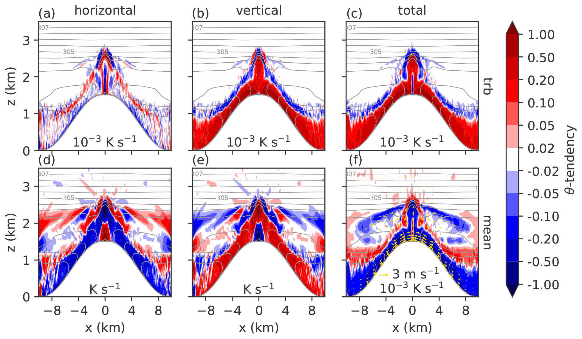
Figure 1Cross sections of total turbulence (trb = resolved + subgrid-scale turbulence, panels a–c) and mean advective (panels d–f) θ tendency components in the Cartesian coordinate system for the averaging period between 3.5 and 4 h after initialization. The calculation is based on Eq. (11), discretized according to Eq. (17), and decomposed with Eqs. (21) and (22). The horizontal (a, d) and vertical (b, e) components are the flux derivatives in the cross-mountain and vertical direction, respectively. Panels (c) and (f) show the sum of the horizontal and vertical components. The units of the color bar are denoted in each panel. Note that a different color scale is used in panels (d) and (e). The contour lines represent mean potential temperature with a spacing of 0.5 K. Panel (f) also shows averaged wind vectors.
The budget components are divided by mean density to obtain tendencies of the form with units of Kelvin per second. This should not be confused with tendencies in advective form 〈∂tθ〉.
We quantify the budget closure with the root-mean-square error of the sum of all forcing terms f with respect to the actual model tendency t normalized by the standard deviation of t:
The averaging is over all grid points and 30 min averaging intervals. Following Chen et al. (2020), we also compute the 99th percentile of the absolute residual scaled by the 99th percentile of the absolute tendency:
4.2 Cross-valley circulation
We start with a short overview of the individual heat budget components in the example simulation for the averaging period between 3.5 and 4 h after initialization.
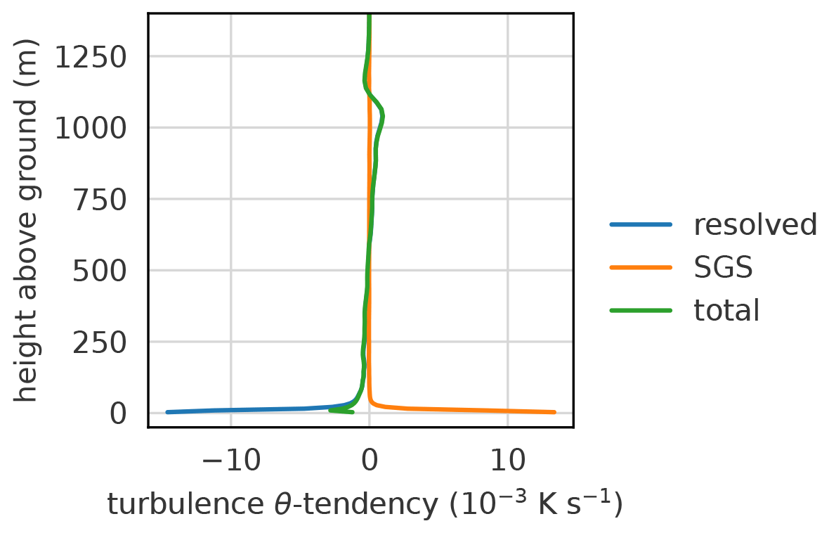
Figure 2Profiles of turbulence θ tendency (subgrid-scale, resolved, and their sum) on the ridge at x=0, for the averaging period between 3.5 and 4 h after initialization.
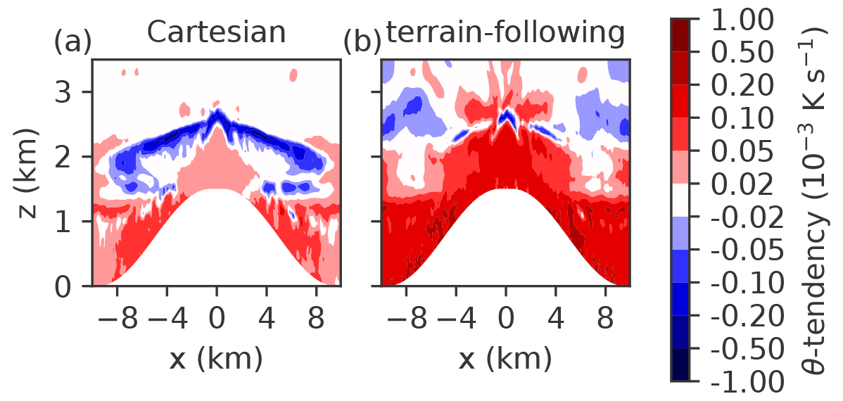
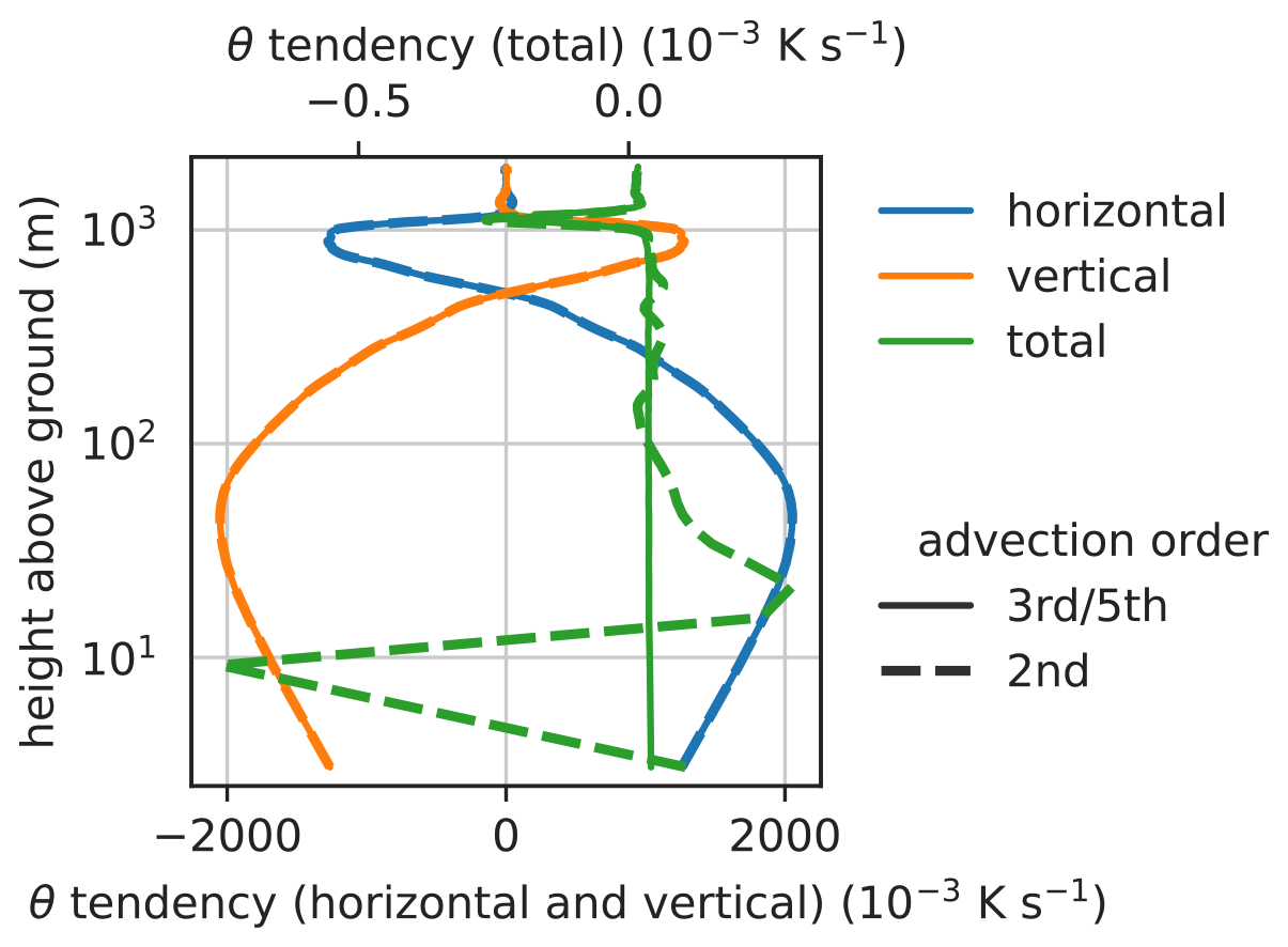
Figure 4Profiles of total θ tendency (resolved + subgrid-scale) on the ridge at x=0, for the averaging period between 3.5 and 4 h after initialization resulting from flux derivatives in the x (blue, lower x axis) and z (orange, lower x axis) directions and their sum (green, upper x axis) calculated with second-order advection (dashed) and third- (vertical) and fifth-order (horizontal) advection, consistent with the numerical model (solid).
Figure 1 shows cross sections of the total turbulence (resolved + subgrid-scale) and mean advective components of the heat budget in the Cartesian coordinate system (Eq. 17). The dynamics are driven by the surface sensible heat flux; vertical turbulent flux convergence in the layer close to the surface (Fig. 1b) induces upslope winds and compensatory return flows aloft and in the valley center (wind arrows in Fig. 1f). Above the slope wind layer, vertical turbulent entrainment leads to cooling (Fig. 1b). Above the ridge, a convective core develops that transports heat from the surface to higher levels. Lateral turbulent entrainment cools the convective core and warms the surrounding air (Fig. 1a). Figure 2 shows the resolved and subgrid-scale turbulence components above the ridge separately. The subgrid-scale component is only relevant close to the ground. There, it causes a positive tendency (flux convergence) by diffusing the sensible heat flux from the ground, while resolved turbulent eddies cause a negative tendency (flux divergence) by transporting the heat further up. The two contributions largely balance out, but the subgrid-scale warming is of slightly lower magnitude than the cooling by the resolved turbulence. The resulting tendency from total turbulence is locally negative; this only occurs within the thermal plume at the ridge top, as visible in Fig. 1c. At all other locations along the slope, the heating by subgrid-scale heat flux convergence offsets the cooling operated by resolved turbulent transport. The mean advective tendency shows regions of horizontal θ flux divergence on the slope and convergence on the ridge and vice versa for the vertical (Fig. 1d and e). These regions essentially coincide with regions of mass convergence and divergence (not shown). The scale of the horizontal and vertical advective tendencies is 3 orders of magnitude larger than for the corresponding turbulence tendencies (Fig. 1a and b). However, the respective sums of the horizontal and vertical components are of comparable magnitude (Fig. 1c and f). Close to the surface, the net mean advective tendency shows cooling of the slope wind layer by the mean upslope wind and warming of the convective core due to horizontal mass convergence (Fig. 1f). The former is weaker than the turbulent heating, while the latter is stronger than the turbulent cooling, leading to net warming close to the surface (Fig. 3a). Away from the surface, the mean advective tendency leads to cooling zones that propagate with time from the ridge towards the valley center. After 4 h this cooling zone spans almost the whole domain in the horizontal direction (Figs. 1f and 3a).
The total tendency in the mass-based terrain-following coordinate system shows somewhat different structures with stronger warming throughout the domain (Fig. 3b). The only difference between the total tendencies in the terrain-following and the Cartesian formulation is the second term on the left-hand side in Eq. (11), which accounts for the height of the vertical levels being time-dependent; the coordinate layers expand as they are heated up. As we can see, this term has a considerable impact and is thus needed to close the budget in Eq. (11). In contrast, in the alternative form of the equation (Eq. 8), the correction term for the time derivative is almost negligible (not shown). With this formulation, Fig. 3a (with correction) and Fig. 3b (without correction) would look almost identical. This shows that the correction terms in Eqs. (11) and (8) are conceptually different, as mentioned in Sect. 2.1.
Since we use the equations in flux form, Figs. 1 and 3, in general, cannot be compared to Schmidli (2013), who used the advective form. However, as Schmidli (2013) points out, under the Boussinesq approximation the total turbulence tendency is equivalent in both formulations. In fact, the total turbulence tendency in Fig. 1c is of comparable magnitude and shows very similar spatial patterns as the one in Fig. 6c in Schmidli (2013).
As shown above, a budget equation typically consists of large competing forcing terms that add up to a relatively small total tendency. To illustrate this, instead of looking at the decomposition into total turbulence and mean advective tendencies as in Fig. 1, we consider the two budget components as they are calculated by the model (not decomposed): resolved advection and subgrid-scale diffusion. The horizontal and vertical components of the resolved advection close to the surface above the ridge are on the order of −1 and +1 K s−1, respectively. Their sum is much smaller: on the order of −10−2 K s−1. The subgrid-scale diffusion is on the order of +10−2 K s−1. Adding the resolved advection and the subgrid-scale diffusion leads to a total tendency on the order of +10−5 K s−1. When adding the large forcing terms, approximations in the budget calculation can lead to considerable errors, as we will demonstrate in the following.
4.3 Comparison of budget calculation methods
We compare the budget obtained with WRFlux (Eq. 17) with several alternative forms. The first alternative uses second-order advection in Eq. (17) instead of the advection order that is consistent with the model (third- and fifth-order). The differences between using second-order and the consistent advection order are largest on the ridge, where the vertical velocities are largest. The horizontal and vertical components of the total θ tendency (resolved + subgrid-scale) in Fig. 4 are both very close for the two calculation methods. But when adding these large and opposing components, the second-order calculation yields considerably different results close to the surface. Instead of the constant warming up to the entrainment layer, we see large oscillations of warming and cooling. The main errors derive from the vertical component (not shown). Only the deviation at 250 originates from errors in the horizontal turbulent entrainment. At other locations in the domain, where the up- and downdrafts are weaker, the differences are smaller.

Figure 5Profiles of resolved turbulence θ tendency over the slope at x = −5 km, for the averaging period between 3.5 and 4 h after initialization resulting from flux derivatives in the x (blue) and z (orange) directions and their sum (green). The line styles indicate different formulations for the horizontal flux derivatives (explained in Sect. 2).
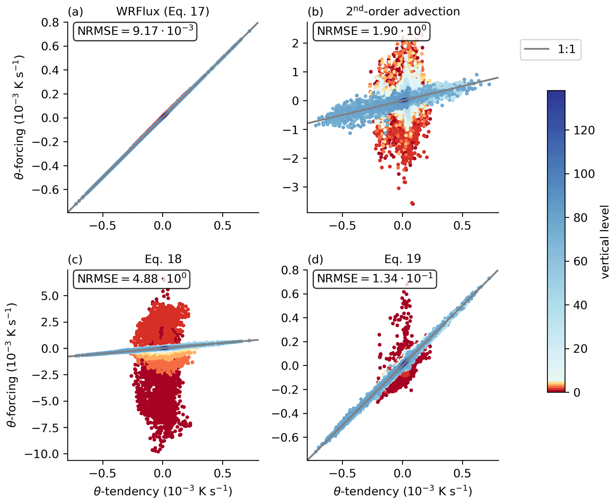
Figure 6Scatterplots of the right-hand side (θ forcing) of Eq. (17), Eq. (17) with second-order advection, Eq. (18), and Eq. (19) against the respective left-hand side (θ tendency) for all model grid points and eight half-hourly (from initialization to 4 h later) values together with the corresponding NRMSE values (Eq. 25). For this plot, the data are only averaged temporally, not spatially. The color code indicates the vertical levels of the model grid points with a focus on the lowest five levels. The gray line is the 1:1 line that signifies a perfectly closed budget.
The different formulations for the horizontal flux derivatives (Sect. 2) differ significantly only where the grid elements are strongly tilted. Figure 5 shows profiles of the resolved turbulence θ tendency over the slope at x = −5 km for the three different formulations. The calculation of the vertical component is identical for all three formulations. The formulation in Eq. (19), which uses the consistently discretized θ in the horizontal correction, yields very similar profiles as the reference WRFlux procedure (Eq. 17). In contrast, the formulation in Eq. (18), in which the horizontally de-staggered and then vertically staggered horizontal flux is used in the corrections, results in considerable errors close to the surface.
Table 1NRMSE (Eq. 25) and r99 (%, Eq. 26) values for all budget variables and budget calculation methods.
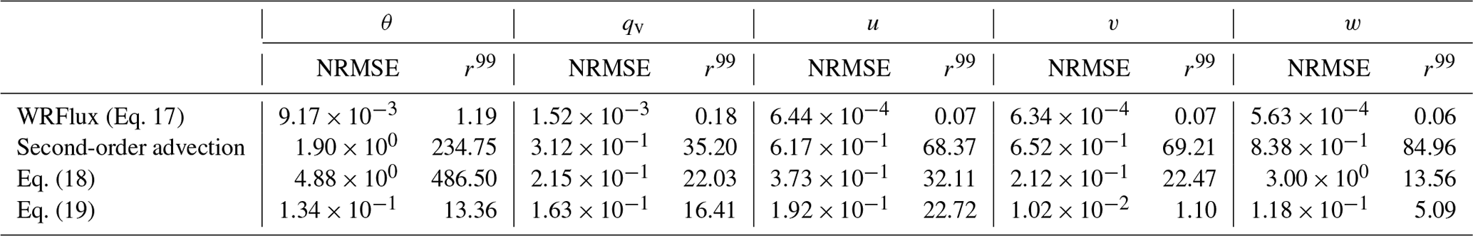
To quantify the differences, we plot the right-hand side (forcing) of Eq. (17), Eq. (17) with second-order advection, Eq. (18), and Eq. (19) against the respective left-hand side (tendency) and compute the normalized root-mean-square error (NRMSE, Eq. 25) in Fig. 6. To avoid averaging out large errors, we drop the spatial averaging for this plot and only use temporal averaging. For the WRFlux procedure (Eq. 17), the points lie close to the 1:1 line, indicating a good budget closure, quantified with an NRMSE of 9.17 × 10⁻³. The NRMSE increases by about 1 order of magnitude when using Eq. (19) and by about 2 orders when using Eq. (18) or second-order advection. The errors are largest at the lowest vertical levels. For the water vapor mixing ratio, the NRMSE of WRFlux is about 6 times smaller and for the wind speed components, it is about 15 times smaller (Table 1). For these variables, the other budget calculation methods lead to NRMSE values that are 2 to 3 orders of magnitude worse than the one of WRFlux.
We also tested two other approximations: using WRF's prognostic vertical velocity in the resolved vertical flux instead of the one recalculated with Eq. (9) and not including the density in the time averaging of the total resolved flux (left-hand side of Eq. 21). The effect on the budget closure is moderate. For both of these approximations, the NRMSE score is increased by about 1 order of magnitude.
To compare our results to Chen et al. (2020), we compute the 99th percentile of the absolute residual scaled by the 99th percentile of the absolute tendency (Eq. 26). For potential temperature, WRFlux reaches a value of r99th≈ 1.2 %. For horizontal momentum (u wind speed), we reach a score of r99th≈ 0.07 %, similar to the value of 0.1 % that Chen et al. (2020) state for their simulations.
We developed a computational method to accurately diagnose the advective and turbulence components of the budgets of prognostic variables in a numerical weather prediction model. The method is based on a numerically consistent implementation of the transformation from a coordinate system with a generalized vertical coordinate, such as a terrain-following coordinate system, to the Cartesian coordinate system. The partitioning of the advective tendency into horizontal and vertical components is different in the two coordinate systems, and thus the coordinate transformation is helpful when investigating the horizontal and vertical components separately. We illustrated this by assessing the local heat budget in a simulation of a convective boundary layer over an idealized 2D mountain ridge. The slope flow layer is subject to vertical resolved and subgrid-scale turbulent heating from the ground and turbulent cooling due to vertical entrainment. Close to the surface, the sum of the potential temperature tendencies due to resolved horizontal and vertical advection is about 2 orders of magnitude smaller than the individual components. Adding the subgrid-scale diffusion yields a total tendency that is another 3 orders of magnitude smaller.
The circumstance of large and counteracting budget components adding up to a relatively small total tendency makes the budget calculation sensitive to approximations. While the sum of all forcing terms in WRFlux agrees to very high precision with the actual model tendency, we could show that approximations based on a lower-order advection operator or a numerically inconsistent formulation of the coordinate transformation lead to large residuals in the budget and noticeable differences in the tendency profiles. When looking at cross-section plots, the differences between the budget calculation methods are hardly noticeable. Nevertheless, a budget analysis tool that yields large residuals is unreliable. In general, if the residual is large, we do not know whether the individual forcing terms are more or less reliable and only the sum is erroneous or whether the forcing terms are not trustworthy either due to approximations or software bugs. Therefore, a closed budget as achieved by WRFlux is essential. This requires the budget calculations to be consistent with the model numerics.
WRFlux expands the approach of Chen et al. (2020) by the computation of resolved turbulence tendencies and the transformation of fluxes and flux divergence components to the Cartesian coordinate system. Possible applications of our budget analysis tool include the study of
-
the reasons for the unclosed surface energy balance often reported in field studies (e.g., De Roo and Mauder, 2018) for which diagnostics in a layer close to the surface are required;
-
the evolution of thermal updrafts in mountainous terrain that are subject to lateral and vertical turbulent entrainment (e.g., Kirshbaum, 2011, 2020);
-
the exchange of heat and moisture between the boundary layer of a valley and the free troposphere (e.g., Rotach et al., 2015; Leukauf et al., 2015, 2017).
A conceivable extension for WRFlux is the inclusion of further budget variables, such as the mixing ratios of other water species or of a passive tracer.
The Jacobian matrix of the transformation from the Cartesian coordinate system to a coordinate system with generalized vertical coordinate η reads
which yields the Jacobian determinant .
The inverse of J is given by
WRFlux is available at https://github.com/matzegoebel/WRFlux (last access: 18 January 2022). The presented example simulation was run with WRFlux v1.2.1 (https://doi.org/10.5281/zenodo.4726600, Göbel, 2021b), which is based on WRF version 4.2.2. Code specific to the example simulation is deposited at https://doi.org/10.5281/zenodo.4724415 (Göbel, 2021a). This upload contains the namelist file, input sounding, and modified initialization routine used for the large-eddy simulation (LES) ideal case in WRF and the simplified radiation scheme introduced in Sect. 4.1.
The post-processed, y-averaged model output data with which Figs. 1–5 can be reproduced are available at https://doi.org/10.5281/zenodo.5879316 (Göbel, 2021c). A simplified plotting script to reproduce the figures is also included in this upload.
MG developed the theoretical framework and the software package, ran and analyzed the example simulation, and prepared the paper. StS and MWR supervised the work and reviewed and edited the paper extensively. StS acquired the funding and administers the project.
The contact author has declared that neither they nor their co-authors have any competing interests.
Publisher's note: Copernicus Publications remains neutral with regard to jurisdictional claims in published maps and institutional affiliations.
The computational results presented have been achieved using the Vienna Scientific Cluster (VSC).
We would like to thank Lukas Umek, Alexander Gohm, and Wiebke Scholz for their suggestions and the many fruitful discussions and Lukas Umek for providing his code (published in Umek et al., 2021), which was the starting point of WRFlux. Last but not least, we thank the three anonymous reviewers for their valuable comments and suggestions.
This research has been supported by the Austrian Science Fund (grant no. P30808-N32).
This paper was edited by James Kelly and reviewed by three anonymous referees.
Arakawa, A. and Lamb, V. R.: Computational Design of the Basic Dynamical Processes of the UCLA General Circulation Model, in: Methods in Computational Physics: Advances in Research and Applications, edited by: Chang, J., vol. 17 of General Circulation Models of the Atmosphere, Elsevier, New York, USA, https://doi.org/10.1016/B978-0-12-460817-7.50009-4, pp. 173–265, 1977. a
Byun, D. W.: Dynamically Consistent Formulations in Meteorological and Air Quality Models for Multiscale Atmospheric Studies. Part I: Governing Equations in a Generalized Coordinate System, J. Atmos. Sci., 56, 3789–3807, https://doi.org/10/bxzs4f, 1999. a, b
Chen, T.-C., Yau, M.-K., and Kirshbaum, D. J.: Towards the closure of momentum budget analyses in the WRF (v3.8.1) model, Geosci. Model Dev., 13, 1737–1761, https://doi.org/10.5194/gmd-13-1737-2020, 2020. a, b, c, d, e, f, g, h, i, j, k
De Roo, F. and Mauder, M.: The influence of idealized surface heterogeneity on virtual turbulent flux measurements, Atmos. Chem. Phys., 18, 5059–5074, https://doi.org/10.5194/acp-18-5059-2018, 2018. a
Deardorff, J. W.: Stratocumulus-Capped Mixed Layers Derived from a Three-Dimensional Model, Bound.-Lay. Meteorol., 18, 495–527, https://doi.org/10/dtgccs, 1980. a
Favre, A.: Statistical Equations of Turbulent Gases, in: Problems of hydrodynamics and continuum mechanics, Society for Industrial and Applied Mathematics, Philadelphia, USA, pp. 231–266, 1969. a
Göbel, M.: Simulation Setup for “Numerically consistent budgets of potential temperature, momentum, and moisture in Cartesian coordinates: application to the WRF model”, Zenodo [code], https://doi.org/10.5281/zenodo.4724415, 2021a. a
Göbel, M.: WRFlux: v1.2.1, Zenodo [code], https://doi.org/10.5281/zenodo.4726600, 2021b. a
Göbel, M.: Model output for “Numerically consistent budgets of potential temperature, momentum and moisture in Cartesian coordinates: Application to the WRF model”, Zenodo [data set], https://doi.org/10.5281/zenodo.5879316, 2021c. a
Greatbatch, R. J.: A Framework for Mesoscale Eddy Parameterization Based on Density-Weighted Averaging at Fixed Height, J. Phys. Oceanogr., 31, 2797–2806, https://doi.org/10/d772sx, 2001. a
Hesselberg, T.: Die Gesetze Der Ausgeglichenen Atmosphärischen Bewegungen, Beiträge zur Physik der Atmosphäre, 12, 141–160, 1926. a
Huang, Y.-H., Wu, C.-C., and Montgomery, M. T.: Concentric Eyewall Formation in Typhoon Sinlaku (2008). Part III: Horizontal Momentum Budget Analyses, J. Atmos. Sci., 75, 3541–3563, https://doi.org/10/gfbrq9, 2018. a
Jiménez, P. A., Dudhia, J., González-Rouco, J. F., Navarro, J., Montávez, J. P., and García-Bustamante, E.: A Revised Scheme for the WRF Surface Layer Formulation, Mon. Weather Rev., 140, 898–918, https://doi.org/10/cm98fw, 2012. a
Kasahara, A.: Various Vertical Coordinate Systems Used for Numerical Weather Prediction, Mon. Weather Rev., 102, 509–522, https://doi.org/10/bh82xh, 1974. a, b, c
Kiranmayi, L. and Maloney, E. D.: Intraseasonal Moist Static Energy Budget in Reanalysis Data, J. Geophys. Res.-Atmos., 116, https://doi.org/10/fcbgw8, 2011. a
Kirshbaum, D. J.: Cloud-Resolving Simulations of Deep Convection over a Heated Mountain, J. Atmos. Sci., 68, 361–378, https://doi.org/10/b8kzbc, 2011. a
Kirshbaum, D. J.: Numerical Simulations of Orographic Convection across Multiple Gray Zones, J. Atmos. Sci., 77, 3301–3320, https://doi.org/10/gjnqnv, 2020. a
Klemp, J. B.: A Terrain-Following Coordinate with Smoothed Coordinate Surfaces, Mon. Weather Rev., 139, 2163–2169, https://doi.org/10/dpd3pb, 2011. a
Klemp, J. B., Dudhia, J., and Hassiotis, A. D.: An Upper Gravity-Wave Absorbing Layer for NWP Applications, Mon. Weather Rev., 136, 3987–4004, https://doi.org/10/d6hwx2, 2008. a
Kowalski, A. S.: Exact Averaging of Atmospheric State and Flow Variables, J. Atmos. Sci., 69, 1750–1757, https://doi.org/10/f3xxh7, 2012. a
Kramm, G., Dlugi, R., and Lenschow, D. H.: A Re-Evaluation of the Webb Correction Using Density-Weighted Averages, J. Hydrol., 166, 283–292, https://doi.org/10/cqpz2t, 1995. a
Lee, T., Fukumori, I., and Tang, B.: Temperature Advection: Internal versus External Processes, J. Phys. Oceanogr., 34, 1936–1944, https://doi.org/10/btgvv8, 2004. a
Lehner, M.: Observations and Large-Eddy Simulations of the Thermally Driven Cross-Basin Circulation in a Small, Closed Basin, PhD thesis, University of Utah, Salt Lake City, USA, available at: https://collections.lib.utah.edu/ark:/87278/s61n8fxw (last access: 18 January 2022), 2012. a
Lehner, M. and Whiteman, C. D.: Physical Mechanisms of the Thermally Driven Cross-Basin Circulation, Q. J. Roy. Meteor. Soc., 140, 895–907, https://doi.org/10/f52kwg, 2014. a
Leukauf, D., Gohm, A., Rotach, M. W., and Wagner, J. S.: The Impact of the Temperature Inversion Breakup on the Exchange of Heat and Mass in an Idealized Valley: Sensitivity to the Radiative Forcing, J. Appl. Meteorol. Clim., 54, 2199–2216, https://doi.org/10/f3sx2n, 2015. a
Leukauf, D., Gohm, A., and Rotach, M. W.: Toward Generalizing the Impact of Surface Heating, Stratification, and Terrain Geometry on the Daytime Heat Export from an Idealized Valley, J. Appl. Meteorol. Clim., 56, 2711–2727, https://doi.org/10/gch62h, 2017. a
Lilly, D. K. and Jewett, B. F.: Momentum and Kinetic Energy Budgets of Simulated Supercell Thunderstorms, J. Atmos. Sci., 47, 707–726, https://doi.org/10/cwpd6k, 1990. a
Liseikin, V. D.: Coordinate Transformations, in: Grid Generation Methods, edited by: Liseikin, V. D., Scientific Computation, Springer Netherlands, Dordrecht, https://doi.org/10.1007/978-90-481-2912-6_2, pp. 31–66, 2010. a, b
Moisseeva, N. and Steyn, D. G.: Dynamical analysis of sea-breeze hodograph rotation in Sardinia, Atmos. Chem. Phys., 14, 13471–13481, https://doi.org/10.5194/acp-14-13471-2014, 2014. a
Pielke, R. A.: Coordinate Transformations, Chapter 6, in: Mesoscale Meteorological Modeling, edited by: Pielke, R. A., Academic Press, San Diego, https://doi.org/10.1016/B978-0-08-092526-4.50009-2, pp. 102–127, 1984. a
Potter, E. R., Orr, A., Willis, I. C., Bannister, D., and Salerno, F.: Dynamical Drivers of the Local Wind Regime in a Himalayan Valley, J. Geophys. Res.-Atmos., 123, 13186–13202, https://doi.org/10/gfrhz7, 2018. a, b
Rampanelli, G., Zardi, D., and Rotunno, R.: Mechanisms of Up-Valley Winds, J. Atmos. Sci., 61, 3097–3111, https://doi.org/10/bgqp3w, 2004. a
Rotach, M. W., Gohm, A., Lang, M. N., Leukauf, D., Stiperski, I., and Wagner, J. S.: On the Vertical Exchange of Heat, Mass, and Momentum Over Complex, Mountainous Terrain, Front. Earth Sci., 3, 76, https://doi.org/10/bxc3, 2015. a
Schmidli, J.: Daytime Heat Transfer Processes over Mountainous Terrain, J. Atmos. Sci., 70, 4041–4066, https://doi.org/10/f5g23h, 2013. a, b, c, d, e, f, g, h
Skamarock, W. C. and Klemp, J. B.: A Time-Split Nonhydrostatic Atmospheric Model for Weather Research and Forecasting Applications, J. Comput. Phys., 227, 3465–3485, https://doi.org/10/cpw3jm, 2008. a
Skamarock, W. C., Klemp, J. B., Dudhia, J., Gill, D. O., Liu, Z., Berner, J., Wang, W., Powers, J. G., Duda, M. G., Barker, D. M., and Huang, X.-Y.: A Description of the Advanced Research WRF Model Version 4, Tech. rep., UCAR/NCAR, Boulder, Colorado, USA, https://doi.org/10.5065/1DFH-6P97, 2019. a, b
Stiperski, I. and Rotach, M. W.: On the Measurement of Turbulence Over Complex Mountainous Terrain, Bound.-Lay. Meteorol., 159, 97–121, https://doi.org/10/f3sz82, 2016. a
Tewari, M., Chen, F., Wang, W., Dudhia, J., LeMone, M. A., Mitchell, K., Ek, M., Gayno, G., Wegiel, J., and Cuenca, R. H.: Implementation and Verification of the Unified Noah Land Surface Model in the WRF Model, in: 20th Conference on Weather Analysis and Forecasting/16th Conference on Numerical Weather Prediction, Seattle, Washington, 14 January 2004, American Meteorological Society, 14.2a, available at: https://ams.confex.com/ams/84Annual/techprogram/paper_69061.htm (last access: 18 January 2022), 2004. a
Umek, L., Gohm, A., Haid, M., Ward, H. C., and Rotach, M. W.: Large-Eddy Simulation of Foehn–Cold Pool Interactions in the Inn Valley during PIANO IOP 2, Q. J. Roy. Meteor. Soc., 147, 944–982, https://doi.org/10/gjgd97, 2021. a, b, c
Xiao, H., Endo, S., Wong, M., Skamarock, W. C., Klemp, J. B., Fast, J. D., Gustafson, W. I., Vogelmann, A. M., Wang, H., Liu, Y., and Lin, W.: Modifications to WRF's Dynamical Core to Improve the Treatment of Moisture for Large-Eddy Simulations, J. Adv. Model. Earth Sy., 7, 1627–1642, https://doi.org/10/gg5jgn, 2015. a
Xue, M. and Lin, S.-J.: Numerical Equivalence of Advection in Flux and Advective Forms and Quadratically Conservative High-Order Advection Schemes, Mon. Weather Rev., 129, 561–565, https://doi.org/10/ckk9vg, 2001. a
This modification is available as a namelist option starting from WRF version 4.3. See https://github.com/wrf-model/WRF/pull/1338 (last access: 18 January 2022).
- Abstract
- Introduction
- Theory
- Implementation
- Example of application and the effect of approximations
- Conclusions
- Appendix A: Coordinate transformation
- Code availability
- Data availability
- Author contributions
- Competing interests
- Disclaimer
- Acknowledgements
- Financial support
- Review statement
- References