the Creative Commons Attribution 4.0 License.
the Creative Commons Attribution 4.0 License.
 | 29 Aug 2022
Impact of the numerical solution approach of a plant hydrodynamic model (v0.1) on vegetation dynamics
L. Ruby Leung
Ryan Knox
Charlie Koven
Ben Bond-Lamberty
Numerous plant hydrodynamic models have started to be implemented in vegetation dynamics models, reflecting the central role of plant hydraulic traits in driving water, energy, and carbon cycles, as well as plant adaptation to climate change. Different numerical approximations of the governing equations of the hydrodynamic models have been documented, but the numerical accuracy of these models and its subsequent effects on the simulated vegetation function and dynamics have rarely been evaluated. Using different numerical solution methods (including implicit and explicit approaches) and vertical discrete grid resolutions, we evaluated the numerical performance of a plant hydrodynamic module in the Functionally Assembled Terrestrial Ecosystem Simulator (FATES-HYDRO version 0.1) based on single-point and global simulations. Our simulation results showed that when near-surface vertical grid spacing is coarsened (grid size >10 cm), the model significantly overestimates aboveground biomass (AGB) in most of the temperate forest locations and underestimates AGB in the boreal forest locations, as compared to a simulation with finer vertical grid spacing. Grid coarsening has a small effect on AGB in the tropical zones of Asia and South America. In particular, coarse surface grid resolution should not be used when there are large and prolonged water content differences among soil layers at depths due to long dry-season duration and/or well-drained soil or when soil evaporation is a dominant fraction of evapotranspiration. Similarly, coarse surface grid resolution should not be used when there is lithologic discontinuity along the soil depth. This information is useful for uncertainty quantification, sensitivity analysis, or the training of surrogate models to design the simulations when computational cost limits the use of ensemble simulations.
- Article
(3828 KB) - Full-text XML
-
Supplement
(834 KB) - BibTeX
- EndNote


Vegetation plays a central role in water, energy, and carbon cycles (Arora, 2002; Gerten et al., 2004; Levis et al., 2000) through the bidirectional interactions between climate and terrestrial biota. Stomatal conductance is one of plants' physiological properties that form the basis of evapotranspiration parameterizations in physically based hydrological models (Arora, 2002) and Earth system models (ESMs). Soil moisture plays a vital role in regulating stomatal conductance and plant water status (Anav et al., 2018; Buckley, 2019). How ESMs represent soil moisture regulation on stomatal conductance thus has important implications for the partitioning of evapotranspiration into evaporation and transpiration, the soil moisture profiles that influence soil hydrological processes, and plant growth and vegetation dynamics, as well as the accurate simulation of land–atmosphere energy and water fluxes.
Most ESMs use non-mechanistic soil moisture stress parameterizations that relate a metric of soil moisture status to attenuation of stomatal conductance in response to declining soil water under drying conditions, ignoring vegetation water use strategies (Kennedy et al., 2019). The ESM community has worked to replace such empirical water stress parameterizations with more realistic mechanistic plant hydrodynamic representations. Water transport in the soil–plant–atmosphere continuum is often represented using a Richards-type equation in the mixed form or potential-based form, which has been commonly used to describe fluid flow in partially saturated porous media (Celia et al., 1990; Lehmann and Ackerer, 1998). In the mixed form, the equation is written using both water potential and water content as the dependent variables, while the equation is written using water potential as the dependent variable in potential-based form. Hydrodynamic representations are nonlinear problems because xylem hydraulic conductivity (Ks) and plant water storage vary nonlinearly with water potential in each organ in the model, so they are typically solved numerically.
Different numerical approaches, with various degrees of simplifications, have been used in the literature to solve the equations in the plant hydrodynamic models. Hydraulic models that consider water storage in the simulated plant organs may use numerical techniques that feature non-iterative (e.g., explicit time integration) or iterative approaches (e.g., Newton's method for nonlinear problems). Examples of models using non-iterative solution approach are the Soil Plant Atmosphere (SPA) model (Williams et al., 1996), a dynamic water flow and storage model called HydGro (Steppe et al., 2006), the trait forest simulator (TFS) (Christoffersen et al., 2016), ED2-hydro (Xu et al., 2016), and Noah-MP-PHS (Li et al., 2021). Models that use iterative solutions include FETCH2 (Mirfenderesgi et al., 2016), the soil plant continuum model (Sperry et al., 1998, 2016), and a porous media model for the hydraulic system (Chuang et al., 2006). There has however been no systematic evaluation and comparison of their model performance and their consequential impact on evapotranspiration partitioning, soil moisture dynamics, and vegetation function and dynamics simulated by the ESMs.
As key differences among different plant hydrodynamic models lie in the numerical approaches used to solve the plant hydrodynamic equations, we implement several numerical solution options for the hydrodynamic problems in the same model to facilitate comparison. The model used here is the plant hydrodynamic model in the Functionally Assembled Terrestrial Ecosystem Simulator (FATES-HYDRO version 0.1) for illustrations. We compare the model performance of the various options and their impacts on simulating evapotranspiration partitioning, soil moisture dynamics, and vegetation dynamics. Our focus is on two aspects of the numerical solutions: vertical grid aggregation of the soil column and use of explicit vs. implicit solvers of the hydrodynamics equations, as they have implications for the accuracy and computational efficiency of the numerical solvers.
2.1 Functionally Assembled Terrestrial Ecosystem Simulator (FATES)
FATES is a vegetation demographic model, which uses the ecosystem demography (ED) (Moorcroft et al., 2001) and perfect-plasticity approximations (PPAs) (Purves et al., 2008) to scale from cohorts of individual plants of different plant functional types growing within a mosaic of patches with different disturbance histories to the land surface (Fisher et al., 2018; Koven et al., 2020). FATES has been coupled to the Energy Exascale Earth System Model (E3SM) land model (ELM) (Golaz et al., 2019; Leung et al., 2020), which we use here. Processes that are simulated in FATES include physiological processes on 30 min time steps, which include photosynthesis, respiration, and radiative transfer, as well as land-surface energy balance and all plant–soil hydrologic calculations coordinated with the land-surface model. At daily timescale, FATES handles plant growth, mortality, and disturbances. More details of FATES can be found in Fisher et al. (2015) and Koven et al. (2020), as well as in the online documentation at https://fates-docs.readthedocs.io/en/latest/fates_tech_note.html (last access: 24 August 2022).
The Energy Exascale Earth System Model (E3SM) is an Earth system model containing components for the atmosphere, land, ocean, sea ice, and rivers (Golaz et al., 2019; Leung et al., 2020). The land model in E3SM, referred to as ELM, was based on the Community Land Model version 4.5 (CLM4.5) (Oleson et al., 2013). The E3SM land model for this study is similar to the Community Land Model version 4.5 (Oleson et al., 2013) except for some biogeochemistry components (Ricciuto et al., 2018; Burrows et al., 2020) and a one-dimensional variably saturated subsurface flow model (Bisht et al., 2018), which were not turned on in this study. In ELM, the soil hydraulic properties are assumed to be a function of sand and clay contents, based on the work by Clapp and Hornberger (1978) and Cosby et al. (1984), and soil organic properties (Lawrence and Slater, 2008). The bulk hydraulic properties are weighted averages of the properties of the soil mineral and organic contents, and details can be found in Oleson et al. (2013). As described in Oleson et al. (2013), the mineral soil texture dataset for each soil layer was created from the International Geosphere-Biosphere Programme (IGBP) soil dataset (Global Soil Data Task, 2000) of 4931 soil mapping units and their sand and clay content (Bonan et al., 2002). The majority of the globe soil organic matter data is from ISRICWISE (Batjes, 2006), and those from the high latitudes come from the 0.25∘ version of the Northern Circumpolar Soil Carbon Database (Hugelius et al., 2013). Both datasets report carbon down to 1 m depth, and carbon is partitioned across the top seven soil layers as in Lawrence and Slater (2008).
2.2 FATES-HYDRO
FATES-HYDRO is an extension of the plant hydrodynamic model described in Christoffersen et al. (2016). It solves transient water flow from soil to roots, stem, and leaf to meet the transpiration demand. Xylem transport in FATES-HYDRO follows Darcy's law, which says that flow rate in the porous media is proportional to the hydraulic gradient and the hydraulic conductivity. FATES-HYDRO accounts for the plant internal water storage that can buffer the imbalance of root water uptake and transpiration demand. In discretized approximation, the transient water mass balance equation along the hydraulic path for each node i can be written as
where i is the node number and i at the leaf node is equal to 1, with nodes ordered from top to bottom and horizontally from the root node to soil node (Fig. 1). Discrete fluxes between the compartment of interest and a total of k other connected compartments are indexed by j. k is 1 for the leaf node, and it is equal to 2 for compartments other than the transporting root compartment, where k equals the number of soil layers plus 1. ρw is the density of water (kg m−3), Vi is the volume of modeled compartment or node (m3), t is time (s), θi is water content (dimensionless), and Qi,j (kg s−1) is the water mass flux between compartments i and j (positive for movement towards the leaf).
The flux over a connection is driven by potential differences between compartments, where g is acceleration due to gravity (9.81 m s−2), and ψi is xylem or soil matric water potential (MPa), which is calculated based on the pressure–volume curve, analogous to the soil water retention curve in ELM soil hydrology (Christoffersen et al., 2016); zi is the elevation above (positive) or below (negative) the ground (m), and Ki is the conductance (kg Mpa−1 s−1) at the boundary between compartments i and j. Ki is calculated as the product of the relative hydraulic conductance kr,i (dimensionless) and the maximum conductance (kg mPa−1 s−1) at the boundary of nodes i. Note the maximum conductance is a product of the conduit cross-section and the material conductivity. Relative conductance or fraction of maximum conductance, kr,i, is calculated by the vulnerability curve using an inverse polynomial function (Manzoni et al., 2013) in plant compartments as follows:
where P50 is the water potential leading to 50 % loss of hydraulic conductivity, and ai is a shape index (dimensionless). The water stress function is usually empirically represented in land models as a function of soil water matric potential, but here it is replaced by an empirical function of leaf water potential to include the hydraulic impacts on stomatal conductance (Christofferson et al., 2016):
where β is a water stress fraction, ψl is the leaf water potential (MPa), P50,gs is the leaf water potential ψl (MPa) at 50 % stomatal closure, and ags is the shape parameter (dimensionless).
β modifies the top of canopy leaf photosynthetic capacity and the Ball–Berry leaf stomatal conductance as shown in Eqs. (5) and (6) below:
where Vc,max is the maximum rate of carboxylation (µmol CO2 m−2 s−1), gs is the leaf stomal conductance (µmol m−2 s−1), m is a parameter that is dependent on the plant functional type, An is leaf net photosynthesis (µmol CO2 m−2 s−1), Cs is the leaf surface CO2 partial pressure (Pa), Patm is the atmospheric pressure (Pa), hs is the leaf surface humidity, b is the minimum stomatal conductance (µmol m−2 s−1), and β is the stress factor defined by Eq. (4).
Hydraulic-failure-induced mortality will be triggered when the plant fractional loss of conductivity (ftc) reaches a threshold (ftc,t, default is 0.5):
where mft is the maximum mortality rate (yr−1), and ftc is the maximum of () for i in plant compartments, where kr,i is defined in Eq. (3).
FATES-HYDRO divides each individual tree into four compartments: leaf, stem, transporting root (troot), and absorbing root (aroot), as shown in Fig. 1. In this study, all compartments except for the absorbing root are represented by a single node for each in the discrete approximation of the equation. The absorbing root is discretized into the same number of nodes as the number of soil layers for soil hydrology in ELM. The soil in each layer is radially discretized into cylindrical shells representing the rhizosphere around an absorbing root (Fig. 1). An example discretization with explicit compartment numbers is shown in Fig. S1 in the Supplement, and Eq. (1) for each compartment is listed in the Supplement as well to demonstrate how each compartment interacts with the others, including the soil–root interaction.
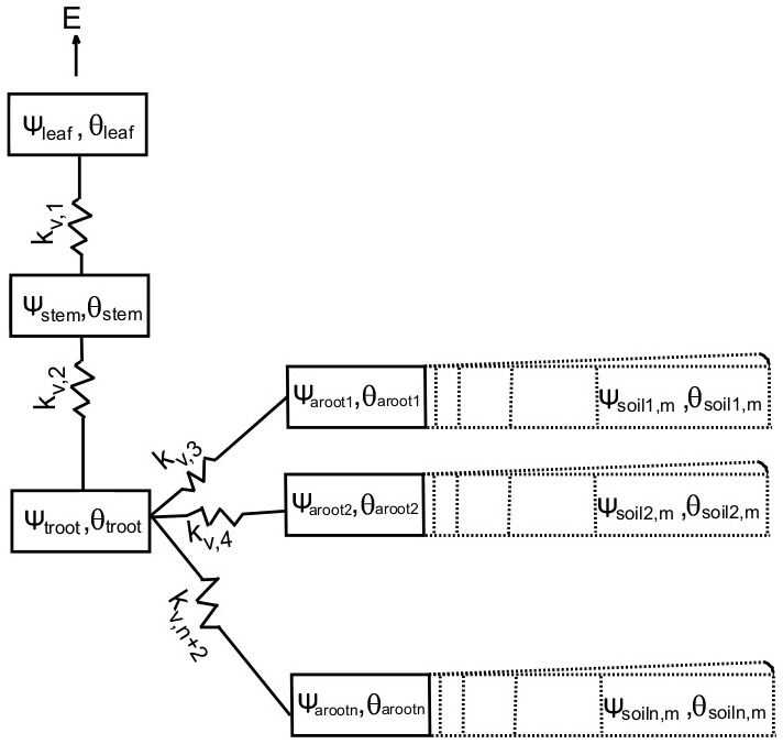
Figure 1Schematic of FATES-hydro, with each box representing a compartment of plant tissue or soil rhizosphere.
2.3 Numerical solutions
We provide the following options to solve Eq. (1), including non-iterative and iterative approaches. For the non-iterative approach, as the time step in FATES for fast processes is 30 min, we use a sub-stepping time integration, with a sub-time step of 10 min, following the time step used in ED2 (Xu et al., 2016). Nonlinear iterative methods, including the Newton and Picard schemes, are commonly used to solve Richards' equation (Albuja and Avila, 2021; Brenner and Cances, 2017; Caviedes-Voullieme et al., 2013; Celia et al., 1990; Lehmann and Ackerer, 1998; List and Radu, 2016). The Picard scheme is a globally convergent method with a low solution efficiency because of its first-order convergence rate. On the other hand, the Newton method is only locally convergent, but a converged solution is not always guaranteed. In this study, we use the Newton method.
We use water content θ in each compartment as unknowns for the Newton iteration. Coupled with a backward Euler approximation in time, the residual form of Eq. (1) for each compartment is defined as
Superscripts n and m denote time level and iteration number, and Rei is the residual for compartment i. The correction quantity δ of water content θ at each point from the last iteration is written as
where δm is the solution of the following matrix equation:
where A is the Jacobian matrix calculated from the derivative of the non-linear function in Eq. (8) with respect to the unknown water content at each compartment, and each row in Eq. (10) is
Taking compartment i connected to compartments i−1 and i+1 as an example, and expanding the water flux in a truncated Taylor series with respect to water content θ at the expansion point , we obtain
Neglecting the higher-order terms, the ith row in Eq. (10) becomes
Equation (10) is solved during each iteration. Convergence of the Newton iteration is achieved when the maximum residual is less than 10−8 or when the following inequality is satisfied at all nodes i:
where τ is the specified tolerance/accuracy. If the scheme is not convergent within the specified maximum number of iterations during a time step, Eq. (1) is explicitly integrated using sub-time stepping within each time step such that the Courant–Friedrichs–Lewy condition (Courant et al., 1928) is below 1.0.
The stack of vertical soil–root interaction layers can be customized by the user to save computation time or carry out a grid convergence study, where a series of grids are generated and model computations are performed to analyze the differences among the results with each grid configuration. In our model configuration, the top soil layer thickness can be as thin as a few centimeters.
Boundary conditions for the system include transpiration flux through leaves and zero flux for the outermost rhizosphere element, assuming the rhizosphere shells encompass the whole soil layer. The rate of water mass change in each soil layer during a time step of FATES-HYDRO is passed to the land model as a source/sink term to calculate the soil water state for the next time step. This rate differs from the transpiration sink as water can be stored or lost in the compartments.
2.4 Grid aggregation
In the default model setting, there are a total of 10 soil layers. Soil layers are the discrete vertical interval over which ELM resolves water content. ELM updates water content via processes of vertical percolation, infiltration, and evaporation and through runoff and drainage of the uppermost and lowermost layers respectively. The water content in each of these layers is presented as an initial condition to FATES-HYDRO. The grid thickness varies from 1.7 cm at the top layer to 1.5 m at the bottom layer. The thickness for layers 2, 3, 4, and 5 is 2.76, 4.55, 7.5, and 12.3 cm, respectively. To reduce computation time and avoid potential numerical stability issues caused by the thin layers, the FATES-HYDRO model can be configured such that several soil layers are aggregated to solve for a fewer number of equations. We define a “rhizosphere layer” as a discrete vertical interval that may contain one or more discrete soil layers, over which the water contents and the fluxes in fine-root tissues are resolved. For simplicity, the depth of the first rhizosphere layer for FATES-HYDRO aligns with the depth of the last soil layer that has been aggregated, and the rest of the rhizosphere layer thickness is the same as that from ELM at the same depth. For example, as shown in Fig. 2, if the first four soil layers (s1 to s4) in ELM are aggregated to form the first rhizosphere layer r1 in FATES-HYDRO, the thickness of r1 is the sum of the thickness of s1 to s4, and the thickness of r2 is the same as s5, and so on. Total water mass in s1 to s4 is assigned to r1. After FATES-HYDRO is solved, the flux exchange between the root and the rhizosphere for r1 is proportionally assigned to s1, s2, s3, and s4, weighted by the product of soil layer thickness and hydraulic conductivity of s1 to s4.
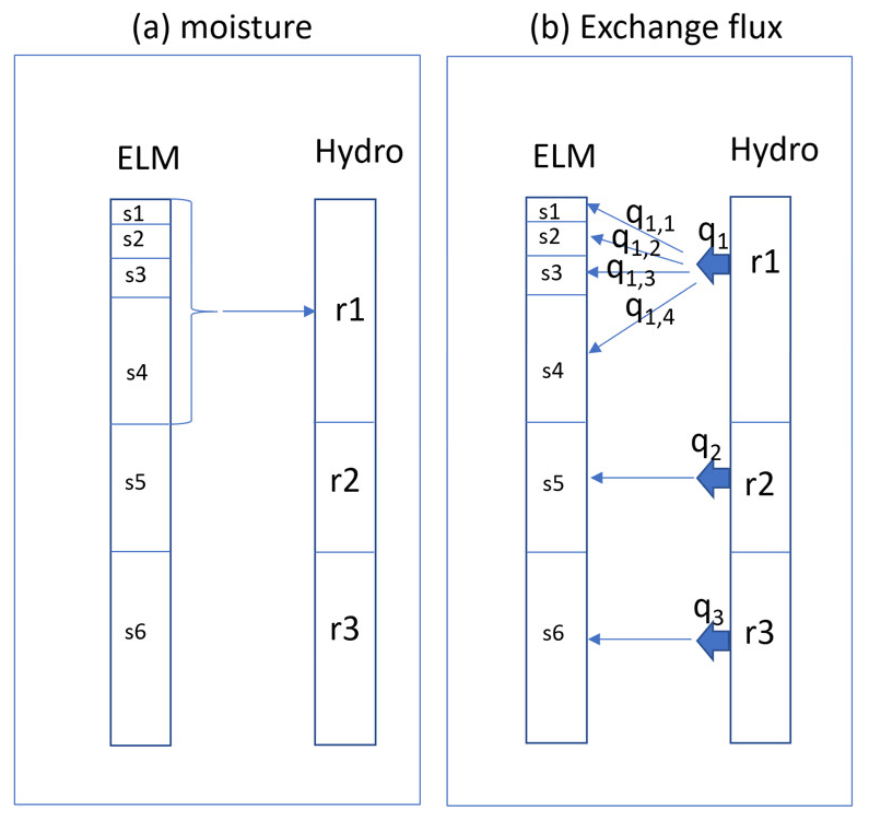
Figure 2Mapping of soil water mass (a) and flux exchange (b) between the soil column in ELM and the rhizosphere in FATES-HYDRO. “s” stands for ELM soil layer, “r” stands for rhizosphere layer, and “q” is flux exchange.
Global and point-scale simulations were performed to assess the impact of vertical soil layer aggregation. A 4×5∘ resolution global simulation was run for 100 years with two rhizosphere grid configurations: (1) no soil layer aggregation (i.e., rhizosphere soil layers in FATES-HYDRO are the same as ELM soil layers), referred to as the Reference case, and (2) aggregation of the top five ELM soil layers, referred to as the Experiment case. A repeating cycle of 3-year (2000–2002) atmospheric forcing data from Qian et al. (2006) is used to drive the model.
Four locations were selected after analyzing the global simulation to further evaluate model performances using different approaches. For point scale at selected locations, simulations with aggregation of one, three, five, and seven layers were first run using the implicit approach to check for model differences in aboveground biomass (AGB). If large differences were found between simulations, extra simulations of different layer aggregations for some points were run to determine which scheme starts to cause large difference and the relative computation costs. Each point was also simulated using the explicit approach for comparison with the implicit approach.
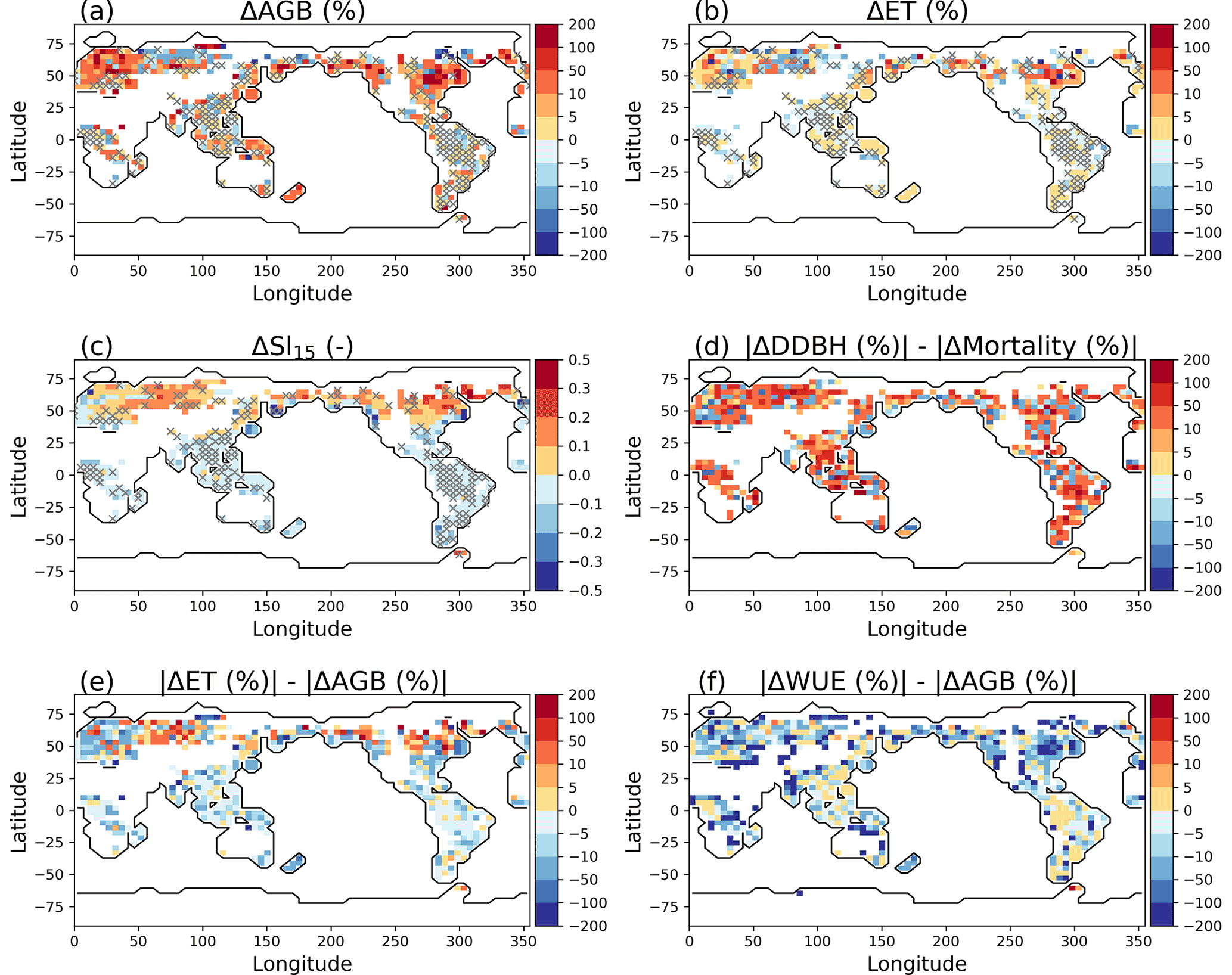
Figure 3Model difference resulted from layer aggregations: percent change of AGB (Experiment − Reference) (a) and percent change of ET (b), average soil water saturation between soil layer 1 and layer 5 in simulation year 100 (c) for the Reference simulation, relative change of growth compared to the relative change of mortality (d), relative change of ET compared to the relative change of AGB (e), and relative change of WUE compared to the relative change of AGB (f). The pixels in white on land have values beyond the limits of the legends, associated with AGB <0.5 gC m−2. Pixels with symbol × have ΔAGB less than 5 %.
3.1 Global simulation
It takes a longer time to solve more equations. The wall clock time for the simulation using no aggregation (Reference case) is 1.5 times that for the simulation using five-layer aggregation (Experiment case). The difference in aboveground biomass (AGB) using different layer aggregation strategies varies by regions, regardless of the total number of simulation years (Fig. 3). It took about 20 d using 120 processor cores to complete 100 years of simulation for the simulation without layer aggregation. Model differences with and without soil layer aggregations were evident during a much earlier simulation year, for example, year 15.
We found that when more rhizosphere soil layers near the surface are aggregated, the Experiment case simulates significantly more AGB (positive ΔAGB in Fig. 3a) in most of the temperate forest locations and less AGB in the boreal forest locations relative to Reference simulation. Layer aggregation only has small effects on AGB (<5 %) in tropical zones near Asia and South America. ΔAGB follows the same pattern as the differences in ET (ΔET) (Fig. 3b). In general, regions with large ΔAGB have small AGB. In the Southern Hemisphere where ΔAGB is high, the annual mean of soil water saturation in the soil layer at the ground surface is generally lower than that in the soil layer 17 cm (layer 5) below the surface (negative soil water saturation differences between soil layer 1 and layer 5 (ΔSl15) in Fig. 3c), and the opposite (positive ΔSl15) is true in a large fraction of the Northern Hemisphere. That is, mixing of soil water from layers of contrasting water saturation when aggregating grids is the main cause of ΔAGB. Using diameter growth increment (DDBH) to represent growth, we compared the difference between the absolute percentage increase of growth and absolute percentage increase of mortality caused by model differences and found mixed influence of growth and mortality on AGB due to soil moisture (Fig. 3d), and there are no specific patterns. However, most of the land pixels show soil moisture has a larger impact on growth than mortality. Compared to the percent change of AGB, the Experiment case has a larger effect on ET (Fig. 3e) in the Northern Hemisphere but an overall small effect on water use efficiency (WUE) (Fig. 3f), which is defined as the ratio of gross primary productivity (GPP) and ET.
Negative soil water saturation differences ΔSl15 between the shallow and deep soil layers can be caused by long dry-season durations and/or when the soil is well drained (rapid decrease of water content with matric potential in the capillary region); regions with large ΔAGB exhibit low clay content and/or long duration of dry seasons (Fig. 4). The dry-season duration is calculated as the number of months when evapotranspiration is larger than precipitation. For example, ΔAGB is big in the temperate forest regions which exhibit large organic matter density compared to the deeper soil layers (Fig. 4f), but the soils in those regions mostly have low and relatively homogeneous clay content (Fig 4c, e). ΔAGB in Amazon is small because of the high clay content (>30 %) and short dry-season durations.
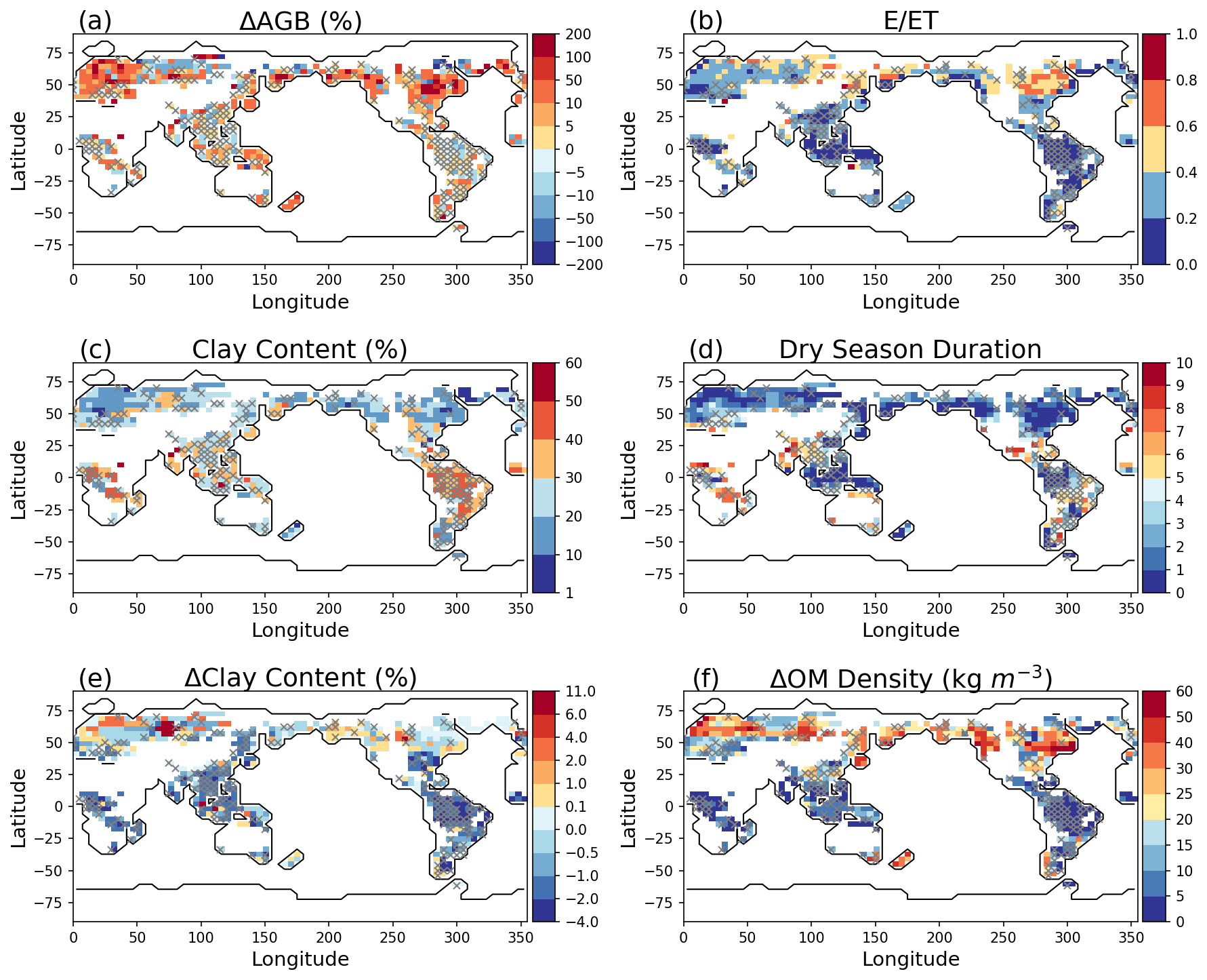
Figure 4Model differences resulted from layer aggregations: percent change of AGB (Experiment − Reference) (a), E ET (b) for simulation year 100, average clay content in the soil column (c), dry-season durations (months) (d), clay content difference (e), and organic matter difference (f) between layer 1 and the average of the top five layers from the surface. The pixels in white on land have values beyond the limits of the legends, associated with AGB <0.5 gC m−2. Pixels with symbol × have AGB differences less than 5 %.
In the high latitudes, layer aggregation schemes can still cause large difference in AGB, even in places with high clay content and short dry-season duration because frozen soil can cause large water content differences in surface soil layers. Ice in the soil can greatly decrease the hydraulic conductivity of the soil through a power law form of the ice-impedance factor, leading to nearly impermeable soil layers (Swenson et al., 2012). A large fraction of the high latitudes has a high soil evaporation / evapotranspiration ratio (E ET) (Fig. 4b). E is determined by the near- surface soil water states, and a large E ET can cause significant water content difference in soil layers. Therefore, the simulated AGB will be significantly changed if the surface soil is aggregated with the deeper wetter soil. Note that this simulation is not calibrated; thus the high E ET at the high latitudes may be overestimated.
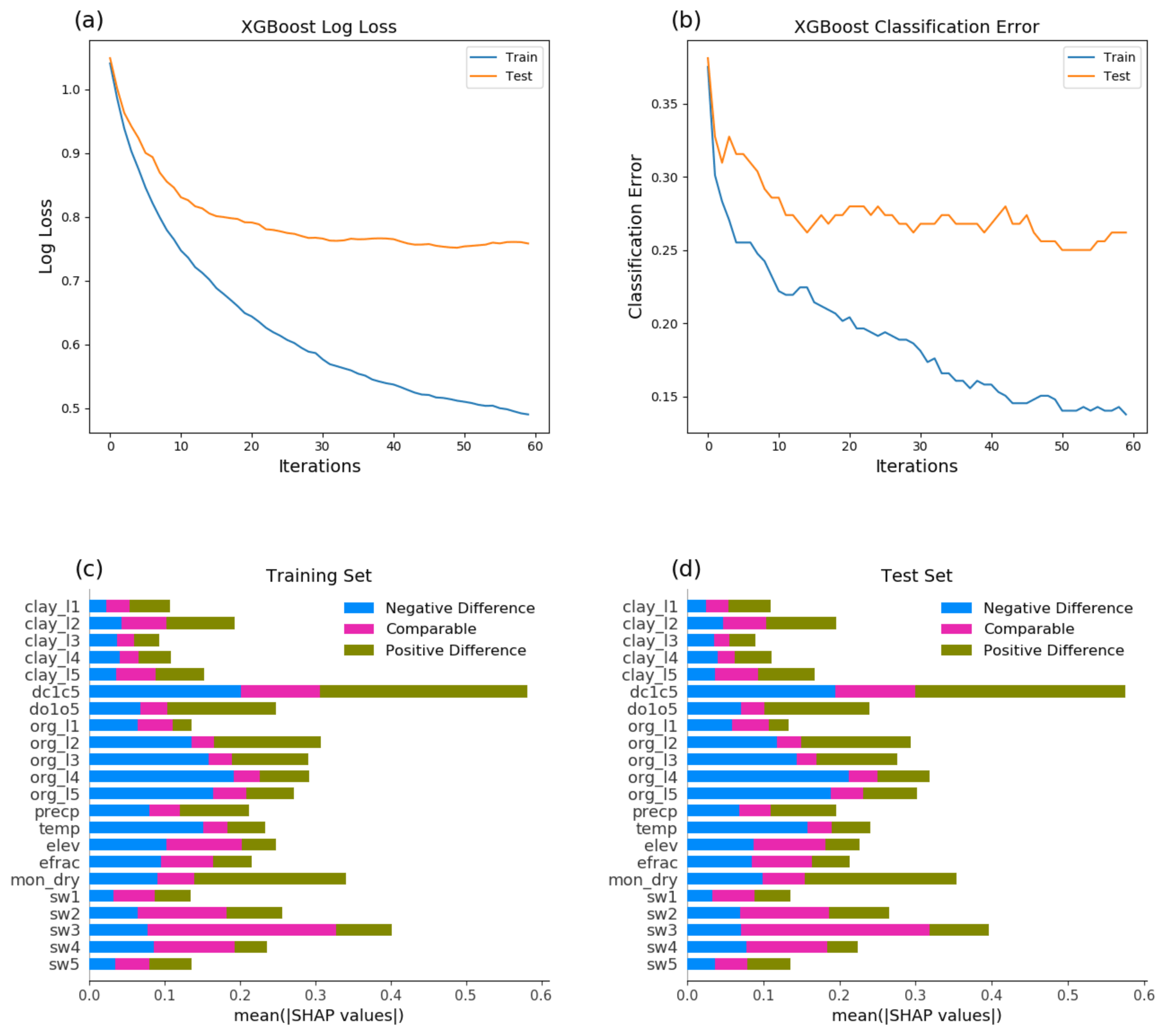
Figure 5XGBoost model evaluation using selected conditions as predictors: learning curve, logarithmic loss (a), learning curve, classification error (b), feature importance for the training set (c), and feature importance for the test set (d).
3.2 Interpretation of the model difference by machine learning
To confirm that the factors such as the E ET ratio and soil property discontinuity along depth are the driving factors for the model differences when aggregating grids in the global simulations, we calculated ΔAGB between the results from the simulation using no layer aggregation and the five-layer aggregation, averaged from the last 5 years of the simulation, and classified the grids with difference greater than 5 % as “positive difference” (i.e., more AGB from the Experiment case), less than −5 % as “negative difference” (i.e., more AGB from the Reference case), and the rest as “comparable”. We then constructed a machine learning model to evaluate the classification skills using the XGBoost classifier from the scikit-learn package in Python and model explanation using SHapley Additive exPlanations (SHAP) by providing impact of features on individual predictions (Lundberg and Lee, 2017). We developed a model using the following inputs including environmental variables: surface elevation, clay content in soil layers 1 to 5 (clay_l1, clay_l2, clay_l3, clay_l4, and clay_l5), clay content difference between the top one and the average of the top five layers (dc1c5), organic matter (OM) density in soil layers 1 to 5 (org_l1, org_l2, org_l3, org_l4, and org_l5), and the OM density difference between the top one and the average of the top five layers (do1o5), precipitation, and temperature, and model-dependent variables – soil evaporation / evapotranspiration ratio (efrac), dry-season duration (mon_dry), and soil water potential from the top five soil layers near the ground surface (sw1, sw2, sw3, sw4, sw5). Clay content and organic matter density were selected as features because they determine hydraulic conductivity. Model-dependent variables were selected to understand the physical process drivers of modeled AGB discrepancy. The machine learning classifier accuracy for the training and test data split from the simulation results is 85 % and 75 %, respectively (Fig. 5). There is 37 % improvement over the theoretical baseline of random guessing, and both training and test data exhibit consistent feature importance.
SHAP feature importance confirmed some of our previous hypothesis explaining the model differences. The top SHAP values for positive model differences in AGB include dc1c5, do1o5, mon_dry, and org_l2, while those responsible for negative model differences are dc1c5, temp, org_l3, org_l4, and org_l5. Temperature becomes important because it affects the presence of soil ice in high latitudes, which affects soil hydraulic conductivity. Features sw3, sw4, dc1c5, and elev are important in explaining small model differences in AGB. Because of the dependencies of efrac and mon_dry on soil moisture and soil hydraulic conductivity (affected by soil texture and ice), it is not surprising that soil water in deep soil layer is important in explaining the model differences. The deep soil water status can affect soil wetness in the rhizosphere soil shell when there is a large contrast between the soil water potential simulated by ELM between the top and deep soil layers.
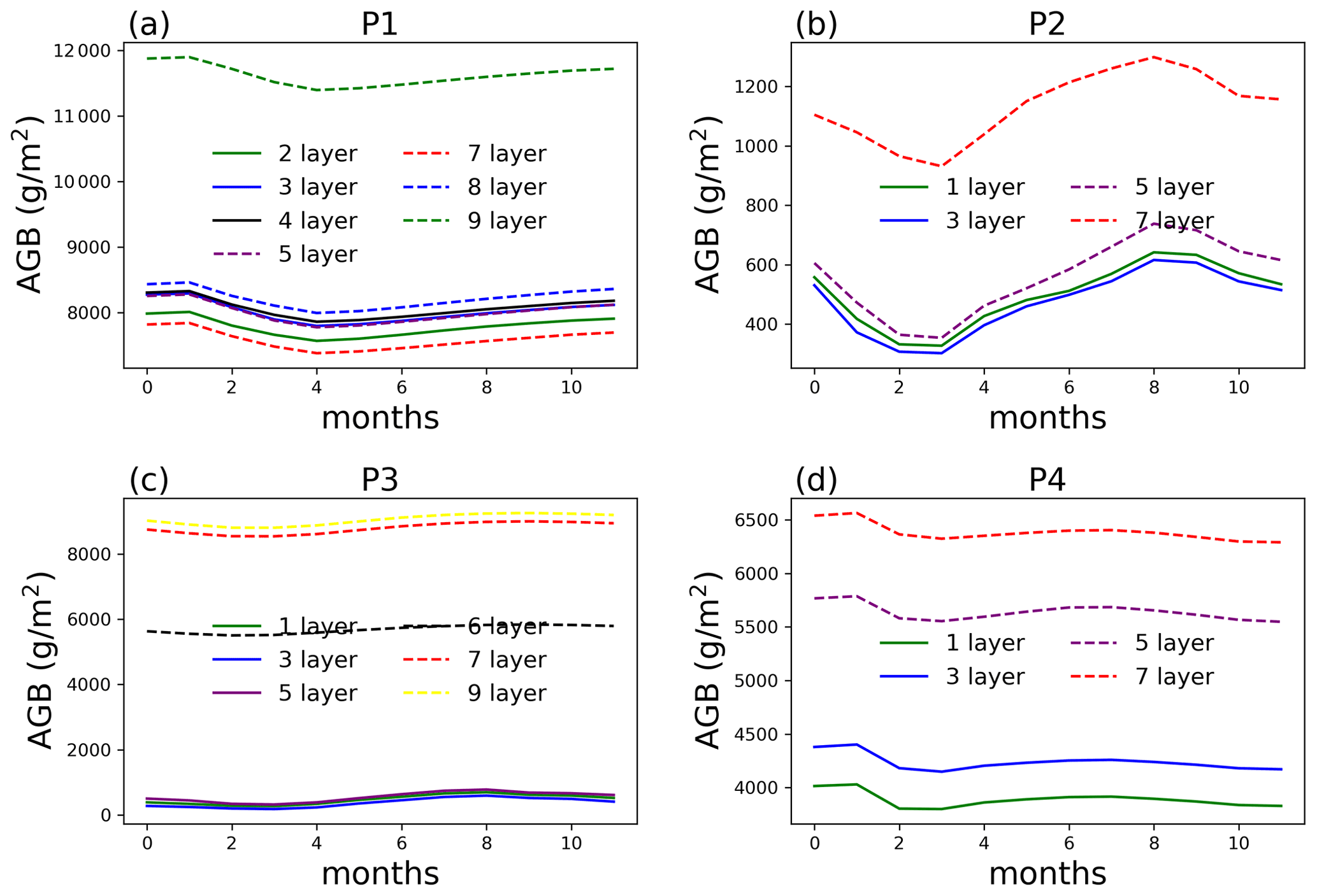
Figure 6AGB from single-point simulations at selected locations (P1–P4) at year 100 of the simulations.
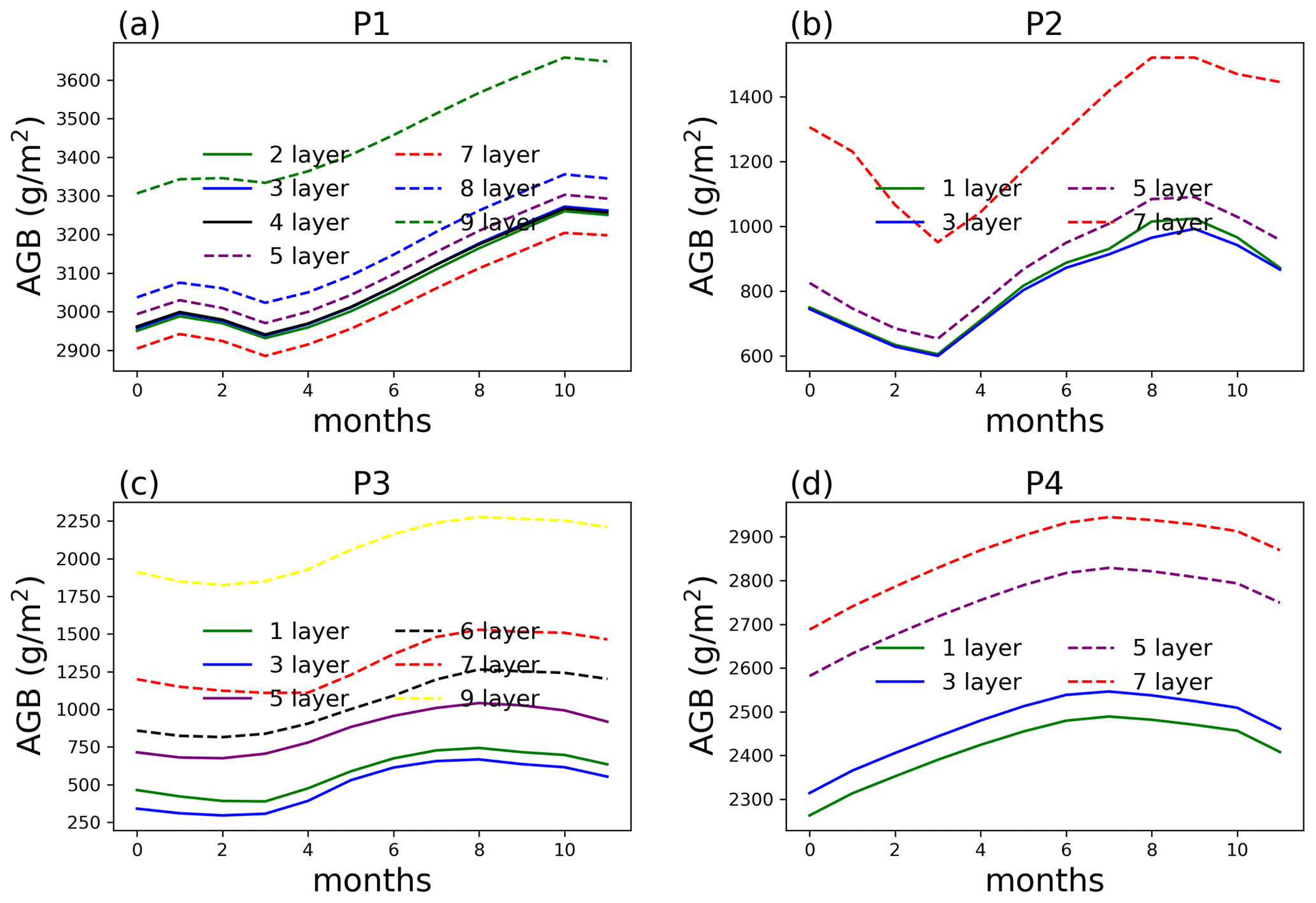
Figure 7AGB from single-point simulations at each selected location (P1–P4) at year 10 of the simulations.
3.3 Single-point simulations
To further understand the effect of soil layer aggregation, we selected a point in the tropical zone (P1, (10∘ N, 80∘ W)), temperate zone (P2, (46∘ N, 95∘ W)), polar zone (P3, (66∘ N, 15∘ E)), and equatorial zone (P4, (6∘ S, 135∘ E)), respectively from the global simulation and ran a 100-year simulation subjecting to a repeating cycle of a 3-year (2000–2002) atmospheric forcing from Qian et al. (2006) at each selected location (Fig. S2). Default FATES-HYDRO parameters are used without modification. Different rhizosphere grid configurations and numerical schemes were run and compared for each point. The clay content and organic matter density at each point are listed in Table S1. At P1 to P3 the clay content is around 30 %, 36 %, and 21 %, respectively, and it varies from 35 % to 26 % from the top to the bottom of soil at P4. Organic matter density varies the most with depth at P3.
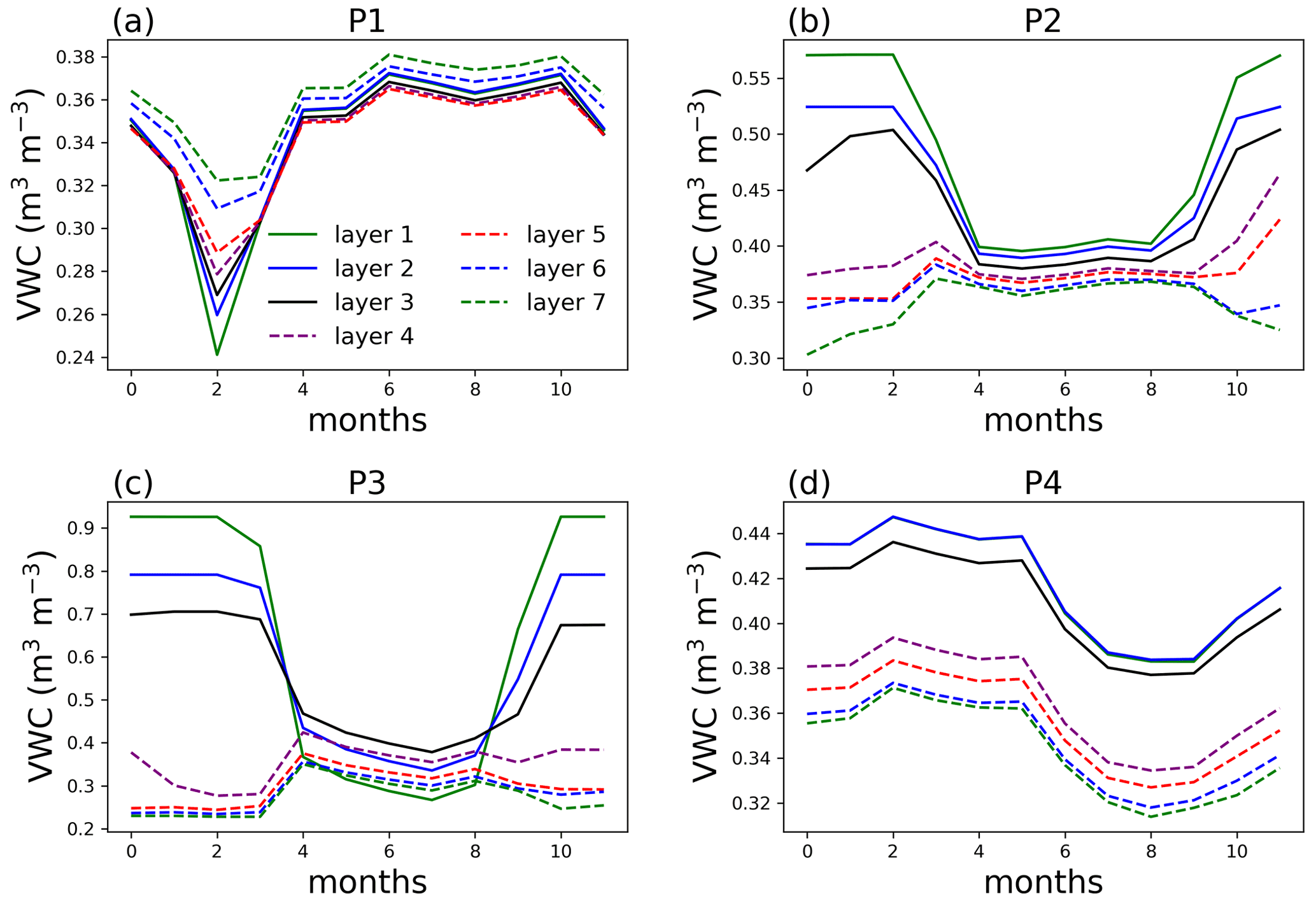
Figure 8Volumetric water content (VWC) at selected points for single-point simulations at year 100 of the simulation with no layer aggregation.
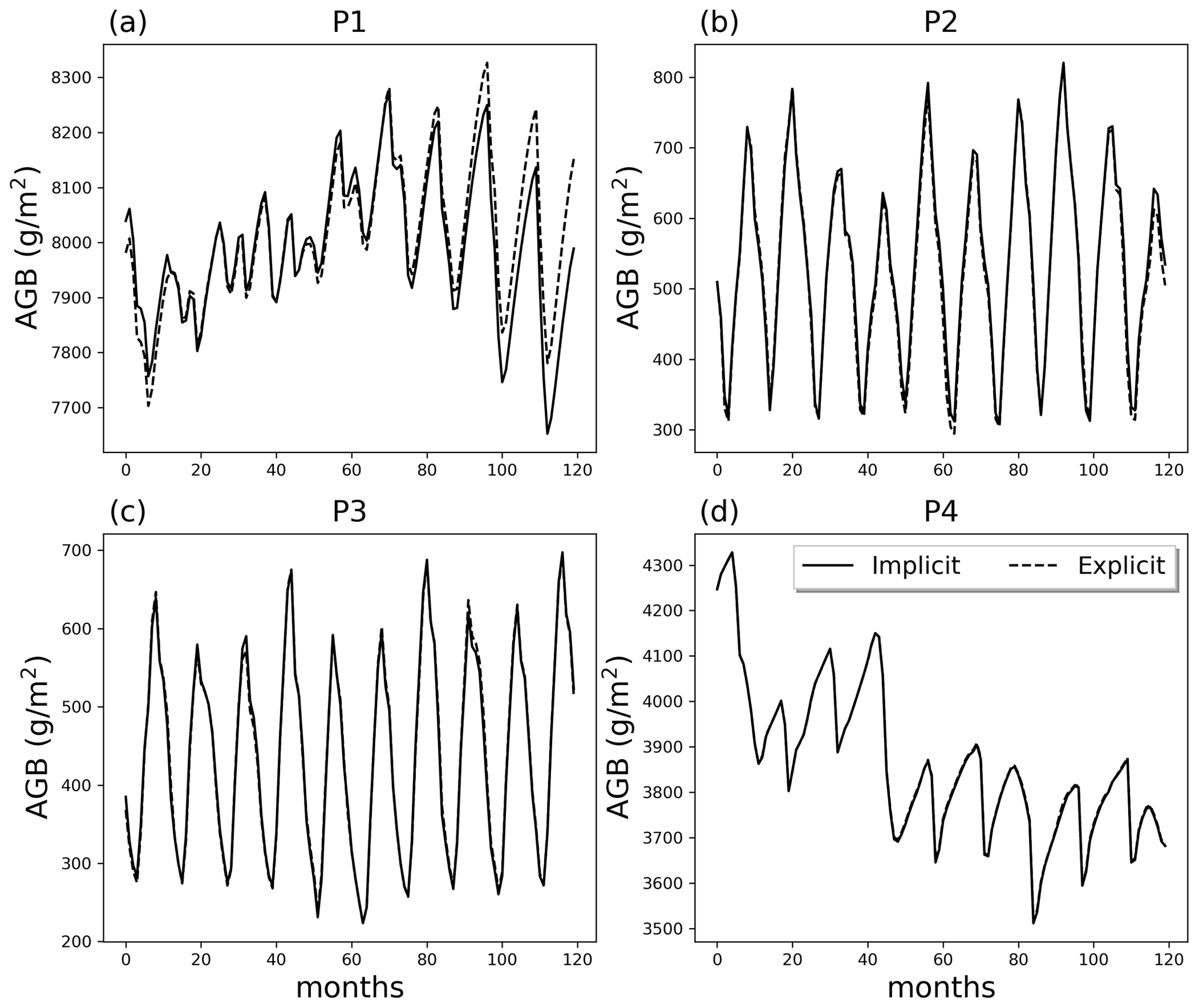
Figure 9Comparison of AGB in the last 10 simulation years at points P1 to P4 with implicit and explicit integration methods.
3.3.1 Aggregation schemes
At the end of the simulation, the fraction of wall clock time of simulations at each point using three-, five-, and seven-layer aggregations are around 0.8, 0.7, and 0.5 times that of the simulation with no layer aggregation.
AGB at point P1 starts to show significant difference (49.3 % on average compared to no aggregation) when only two rhizosphere layers are simulated, i.e., aggregating the top nine layers for the surface soil (Fig. 6). For P2, aggregating five layers and more can result in more than 12 % of AGB difference compared to no aggregation. The same is true for points P3 and P4, with larger differences for more layer aggregation. This kind of AGB difference between different layer aggregation schemes shows up early in the simulation, as shown in Fig. 7 for the 10-year simulation comparison. This means one does not need to run the full simulation to test whether layer aggregation will cause large AGB errors if computation cost is a concern. We found at these four sites, ET (Fig. S3) and WUE (Fig. S4) are not as significantly affected by layer aggregations as AGB.
At P1, the largest difference in water content is in February, the driest month, while the difference is trivial in the other months (Fig. 8). Because the dry-season duration is short, and clay content is relatively homogeneous at P1, aggregating the surface layers at this point does not cause large difference in AGB. Layers 4 and deeper at P2 and P3 are affected by ice impedance, creating a large difference from the top three layers. The water content at P3 is also affected by the large contrast in organic matter density between the surface layer and deeper soil from layer 4. At P4, lithologic discontinuity (clay content separation) between the top three layers and bottom layers can cause inaccuracy in soil water content and hence AGB.
Note that the response of AGB to the number of soil layers aggregated is nonlinear because of the nonlinearity of soil water retention curve and plant vulnerability curve and different layer soil properties, which will consequentially affect when growth or mortality will be more affected by the changing soil water status.
3.3.2 Integration methods
Implicit and explicit integrations of Eq. (1) for points P1 to P4 were run to evaluate model performance and computation costs. The simulations were performed without layer aggregation for comparison of the integration schemes. The time step for the explicit integration is 10 min. There are discrepancies between the two integration approaches at P1, but results show less than 2 % AGB difference at the end of the simulation year (Fig. 9). Results at P2 to P4 are almost identical. However, simulations took more time using the explicit integration approach, with wall clock times 1.85, 1.31, 1.93, and 1.72 times that of the implicit integration for P1 to P4, respectively.
Note that FATES is part of an Earth system model, which is expected to predict plant–soil hydraulic fluxes in innumerable conditions and extremes, over potentially long periods of time. The explicit approach is easier to implement than the implicit approach in terms of coding. However, the explicit approach tends to have stability issues and requires small time steps, while the implicit approach is stable using large time steps but may require many iterations to converge to a solution. We acknowledge there are other solvers that have been used effectively in hydraulic simulations (e.g., Crank–Nicolson), but there is often no best solver. The hydraulic solvers in this study were chosen based on the need to prioritize numerical stability for long simulations, which de-emphasizes the use of explicit solvers. The numerical experiments with different integration schemes in this study can serve as benchmark against each other. In the meantime, it shows that the 10 min time step in ED2 (Xu et al., 2016) is a reasonable time step for these single-point tests, but it is always a good practice to do convergence and stability tests for a specific study. As a matter of fact, our 1-year global simulation for the Reference case using the explicit integration and 10 min time step can result in more than 10 % of AGB difference compared to the implicit approach.
We have implemented multiple numerical schemes in solving plant hydrodynamic equations, including explicit and implicit iterative integration of Eq. (1), as well as aggregated rhizosphere soil layers for the consideration of computation cost and numerical difficulties. While not exhaustive, our results showed that explicit integration using a 10 min time step results in comparable AGB with the implicit method but has a longer simulation time. We also found that care should be taken when configuring soil layering as it can significantly affect AGB results. Large water content differences among soil layers at depth can occur due to lithologic discontinuity, long dry-season duration, high E ET ratio, or well-drained soil. Short time simulation tests can be sufficient to evaluate how model configurations or numerical approaches will affect the simulated AGB accuracy. The cost and accuracy using alternative grid aggregation methods (e.g., fewer number of cylindrical shells) and the approach to pass flux from aggregated layers back to ELM soil layers can be further investigated in the future. The results from our analysis are useful for uncertainty quantification, sensitivity analysis, or the training of surrogate models to design the simulations when computation cost limits the selection of ensemble simulations.
The FATES-HYDRO code is available at https://doi.org/10.5281/zenodo.6461878 (Fang et al., 2022).
The supplement related to this article is available online at: https://doi.org/10.5194/gmd-15-6385-2022-supplement.
YF, RK, and CK developed the code. YF set up the model, performed simulations, and prepared the figures. YF, LRL, RK, CK, and BBL contributed to writing and editing.
The contact author has declared that none of the authors has any competing interests.
Publisher's note: Copernicus Publications remains neutral with regard to jurisdictional claims in published maps and institutional affiliations.
The Pacific Northwest National Laboratory (PNNL) is operated for DOE by Battelle Memorial Institute under contract DE-AC05-76RLO1830.
This research was supported by the U.S. Department of Energy Office of Science Biological and Environmental Research through the Earth System Development program as part of the Energy Exascale Earth System Model (E3SM) project (grant no. 65814).
This paper was edited by Hisashi Sato and reviewed by Gil Bohrer and one anonymous referee.
Albuja, G. and Avila, A. I.: A family of new globally convergent linearization schemes for solving Richards' equation, Appl. Numer. Math, 159, 281–296, https://doi.org/10.1016/j.apnum.2020.09.012, 2021.
Anav, A., Proietti, C., Menut, L., Carnicelli, S., De Marco, A., and Paoletti, E.: Sensitivity of stomatal conductance to soil moisture: implications for tropospheric ozone, Atmos. Chem. Phys., 18, 5747–5763, https://doi.org/10.5194/acp-18-5747-2018, 2018.
Arora, V.: Modeling vegetation as a dynamic component in soil-vegetation-atmosphere transfer schemes and hydrological models, Rev. Geophys., 40, 1–26, https://doi.org/10.1029/2001rg000103, 2002.
Batjes, N. H.: ISRIC-WISE derived soil properties on a 5 by 5 arc-minutes global grid, Report 2006/02, http://www.isric.org (last access: 24 August 2022), 2006.
Bisht, G., Riley, W. J., Hammond, G. E., and Lorenzetti, D. M.: Development and evaluation of a variably saturated flow model in the global E3SM Land Model (ELM) version 1.0, Geosci. Model Dev., 11, 4085–4102, https://doi.org/10.5194/gmd-11-4085-2018, 2018.
Bonan, G.B., Levis, S., Kergoat, L., and Oleson, K. W.: Landscapes as patches of plant functional types: An integrating concept for climate and ecosystem models, Global Biogeochem. Cy., 16, 5.1–5.23, https://doi.org/10.1029/2000GB001360, 2002.
Brenner, K. and Cances, C.: Improving Newton's Method Performance by Parametrization: The Case of the Richards Equation, Siam J. Numer. Anal., 55, 1760–1785, https://doi.org/10.1137/16m1083414, 2017.
Buckley, T. N.: How do stomata respond to water status?, New Phytol., 224, 21–36, https://doi.org/10.1111/nph.15899, 2019.
Burrows, S. M., Maltrud, M., Yang, X., Zhu, Q., Jeffery, N., Shi, X., Ricciuto, D., Wang, S., Bisht, G., Tang, J., Wolfe, J., Harrop, B. E., Singh, B., Brent, L., Baldwin, S., Zhou, T., Cameron-Smith, P., Kneen, N., Collier, N., Xu, M., Hunke, E. C., Elliott, S. M., Turner, A. K., Li, H., Wang, H., Gloaz, J. C., Bond-Lamberty, B., Hoffman, F. M., Riley, W. J., Thornton, P. E., Calvin, K., and Leung, L. R.: The DOE E3SM v1.1 Biogeochemistry Configuration: Description and Simulated Ecosystem-Climate Responses to Historical Changes in Forcing, J. Adv. Model. Earth. Sy., 12, e2019MS001766, https://doi.org/10.1029/2019MS001766, 2020.
Caviedes-Voullieme, D., Garcia-Navarro, P., and Murillo, J.: Verification, conservation, stability and efficiency of a finite volume method for the 1D Richards equation, J. Hydrol., 480, 69–84, https://doi.org/10.1016/j.jhydrol.2012.12.008, 2013.
Celia, M. A., Bouloutas, E. T., and Zarba, R. L.: A General Mass-Conservative Numerical-Solution for the Unsaturated Flow Equation, Water Resour. Res., 26, 1483–1496, https://doi.org/10.1029/WR026i007p01483, 1990
Christoffersen, B. O., Gloor, M., Fauset, S., Fyllas, N. M., Galbraith, D. R., Baker, T. R., Kruijt, B., Rowland, L., Fisher, R. A., Binks, O. J., Sevanto, S., Xu, C., Jansen, S., Choat, B., Mencuccini, M., McDowell, N. G., and Meir, P.: Linking hydraulic traits to tropical forest function in a size-structured and trait-driven model (TFS v.1-Hydro), Geosci. Model Dev., 9, 4227–4255, https://doi.org/10.5194/gmd-9-4227-2016, 2016.
Clapp, R. B. and Hornberger, G. M.: Empirical Equations for Some Soil Hydraulic-Properties, Water Resour. Res., 14, 601–604, https://doi.org/10.1029/Wr014i004p00601, 1978.
Cosby, B. J., Hornberger, G. M., Clapp, R. B., and Ginn, T. R.: A statistical exploration of the relationships of soil moisture characteristics to the physical properties of soils, Water Resour. Res., 20, 682–690, https://doi.org/10.1029/WR020i006p00682, 1984.
Chuang, Y. L., Oren, R., Bertozzi, A. L., Phillips, N., and Katul, G. G.: The porous media model for the hydraulic system of a conifer tree: Linking sap flux data to transpiration rate, Ecol. Model., 191, 447–468, https://doi.org/10.1016/j.ecolmodel.2005.03.027, 2006.
Courant, R., Friedrichs, K., and Lewy, H.: Über die partiellen Differenzengleichungen der mathematischen Physik, Math. Ann., 100, 32–74, 1928.
Fang, Y., Leung, R., Knox, R., Koven, C., and Bond-Lamberty, B.: FATES-HYDRO, Zenodo [code], https://doi.org/10.5281/zenodo.6461878, 2022.
Fisher, R. A., Muszala, S., Verteinstein, M., Lawrence, P., Xu, C., McDowell, N. G., Knox, R. G., Koven, C., Holm, J., Rogers, B. M., Spessa, A., Lawrence, D., and Bonan, G.: Taking off the training wheels: the properties of a dynamic vegetation model without climate envelopes, CLM4.5(ED), Geosci. Model Dev., 8, 3593–3619, https://doi.org/10.5194/gmd-8-3593-2015, 2015.
Fisher, R. A., Koven, C. D., Anderegg, W. R. L., Christoffersen, B. O., Dietze, M. C., Farrior, C. E., Holm, J. A., Hurtt, G. C., Knox, R. G., Lawrence, P. J., Lichstein, J. W., Longo, M., Matheny, A. M., Medvigy, D., Muller-Landau, H. C., Powell, T. L., Serbin, S. P., Sato, H., Shuman, J. K., Smith, B., Trugman, A. T., Viskari, T., Verbeeck, H., Weng, E., Xu, C., Xu, X., Zhang, T., and Moorcroft, P. R.: Vegetation demographics in Earth System Models: A review of progress and priorities, Global Change Biol., 24, 35–54, https://doi.org/10.1111/gcb.13910, 2018.
Gerten, D., Schaphoff, S., Haberlandt, U., Lucht, W., and Sitch, S.: Terrestrial vegetation and water balance – hydrological evaluation of a dynamic global vegetation model, J. Hydrol., 286, 249–270, https://doi.org/10.1016/j.jhydrol.2003.09.029, 2004.
Global Soil Data Task 2000: Global soil data products CD-ROM (IGBP-DIS). International Geosphere-Biosphere Programme-Data and Information Available Services, https://daac.ornl.gov/SOILS/guides/IGBP-DIS.html (last access: 24 August 2022), 2000.
Golaz, J. C., Caldwell, P. M., Van Roekel, L. P., Petersen, M. R., Tang, Q., Wolfe, J. D., Valentine Anantharaj, G. A., Asay-Davis, X. S., Bader, D. C., Baldwin, S. A., Bisht, G., Bogenschutz, P. A., Branstetter, M., Brunke, M. A., Brus, S. R., Burrows S. M., Cameron-Smith, P. J., Donahue, A. S., Deakin, M., Easter, R. C., Evans K. J., Feng, Y., Flanner M., Foucar, J. G., Fyke, J. G., Griffin, B. M., Hannay, C., Harrop, B. E., Hoffman, M. J., Hunke, E. C., Jacob, R. L., Jacobsen, D. W., Jeffery, N., Jones, P. W., Keen, N. D., Klein, S. A., Larson, V. E., Leung, L. R., Li, H., Lin, W., Lipscomb, W. H., Ma, P. L., Mahajan, S., Maltrud, M. E., Mametjanov, A., McClean, J. L, McCoy, R. B., Neale, R. B., Price, S. F., Qian, Y., Rasch, P. J., Eyre, J. E. J. R, Riley, W. J., Ringler, T. D., Roberts, A. F., Roesler, E. L., Salinger, A. G., Shaheen, Z. Shi, X., Singh, B., Tang, J., Taylor, M. A., Thornton, P. E., Turner, A. K., Veneziani, M., Wan, H., Wang, H., Wang, S., Williams, D. N., Wolfram, P. J., Worley, P. H., Xie, S., Yang, Y., Yoon, J., Zelinka, M. D., Zender, C. S., Zeng, X., Zhang, C., Zhang, K., Zhang, Y., Zheng, X., Zhou, T., and Zhu, Q.: The DOE E3SM Coupled Model Version 1: Overview and Evaluation at Standard Resolution, J. Adv. Model. Earth Sy., 11, 2089–2129, https://doi.org/10.1029/2018ms001603, 2019
Hugelius, G., Tarnocai, C., Broll, G., Canadell, J. G., Kuhry, P., and Swanson, D. K.: The Northern Circumpolar Soil Carbon Database: spatially distributed datasets of soil coverage and soil carbon storage in the northern permafrost regions, Earth Syst. Sci. Data, 5, 3–13, https://doi.org/10.5194/essd-5-3-2013, 2013.
Kennedy, D., Swenson, S., Oleson, K. W., Lawrence, D. M., Fisher, R., da Costa, A. C. L., and Gentine, P.: Implementing Plant Hydraulics in the Community Land Model, Version 5, J. Adv. Model. Earth Sy., 11, 485–513, https://doi.org/10.1029/2018ms001500, 2019.
Koven, C. D., Knox, R. G., Fisher, R. A., Chambers, J. Q., Christoffersen, B. O., Davies, S. J., Detto, M., Dietze, M. C., Faybishenko, B., Holm, J., Huang, M., Kovenock, M., Kueppers, L. M., Lemieux, G., Massoud, E., McDowell, N. G., Muller-Landau, H. C., Needham, J. F., Norby, R. J., Powell, T., Rogers, A., Serbin, S. P., Shuman, J. K., Swann, A. L. S., Varadharajan, C., Walker, A. P., Wright, S. J., and Xu, C.: Benchmarking and parameter sensitivity of physiological and vegetation dynamics using the Functionally Assembled Terrestrial Ecosystem Simulator (FATES) at Barro Colorado Island, Panama, Biogeosciences, 17, 3017–3044, https://doi.org/10.5194/bg-17-3017-2020, 2020.
Lawrence, D. M. and Slater, A. G.: Incorporating organic soil into a global climate model, Clim. Dyn., 30, 145–160, https://doi.org/10.1007/s00382-007-0278-1, 2008.
Lehmann, F. and Ackerer, P. H.: Comparison of iterative methods for improved solutions of the fluid flow equation in partially saturated porous media, Transport Porous Med., 31, 275–292, https://doi.org/10.1023/A:1006555107450, 1998.
Leung, L. R., Bader, D. C., Taylor, M. A., and McCoy, R. B.: An Introduction to the E3SM Special Collection: Goals, Science Drivers, Development, and Analysis, J. Adv. Model. Earth Sy., 12, e2019MS001821, https://doi.org/10.1029/2019MS001821, 2020.
Levis, S., Foley, J. A., and Pollard, D.: Large-scale vegetation feedbacks on a doubled CO2 climate, J. Climate, 13, 1313–1325, https://doi.org/10.1175/1520-0442(2000)013<1313:Lsvfoa>2.0.Co;2, 2000.
Li, L. Yang, C., Z. L., Matheny, A. M., Zheng, H., Swenson, S. C., Lawrence, D. M., Barlage, M., Yan, B. Y., McDowell, N. G., and Leung, L. R.: Representation of Plant Hydraulics in the Noah-MP Land Surface Model: Model Development and Multiscale Evaluation, J. Adv. Model. Earth Sy., 13, e2020MS002214, https://doi.org/10.1029/2020MS002214, 2021.
List, F. and Radu, F. A.: A study on iterative methods for solving Richards' equation, Computat. Geosci., 20, 341–353, https://doi.org/10.1007/s10596-016-9566-3, 2016.
Lundberg, S. M. and Lee, S. I.: A Unified Approach to Interpreting Model Predictions, Adv. Neur. In., 30, 4768–4777, https://doi.org/10.48550/arXiv.1705.07874, 2017.
Manzoni, S., Vico, G., Katul, G., Palmroth, S., Jackson, R. B., and Porporato, A.: Hydraulic limits on maximum plant transpiration and the emergence of the safety-efficiency trade-off, New Phytol., 198, 169–178, https://doi.org/10.1111/nph.12126, 2013.
Mirfenderesgi, G., Bohrer, G., Matheny, A. M., Fatichi, S., Frasson, R. P. D., and Schafer, K. V. R.: Tree level hydrodynamic approach for resolving aboveground water storage and stomatal conductance and modeling the effects of tree hydraulic strategy, J. Geophys. Res.-Biogeo., 121, 1792–1813, https://doi.org/10.1002/2016jg003467, 2016.
Moorcroft, P. R., Hurtt, G. C., and Pacala, S. W.: A method for scaling vegetation dynamics: The ecosystem demography model (ED), Ecol. Monogr., 71, 557–585, https://doi.org/10.1890/0012-9615(2001)071[0557:Amfsvd]2.0.Co;2, 2001.
Oleson, K., Lawrence, D. M., Bonan, G. B., Drewniak, B., Huang, M., Koven, C. D., Levis, S., Li, F., Riley, W.J., Subin, Z. M. Swenson, S. C., Thornton, P. E., Bozbiyik, A., Fisher, R., Heald, C.L., Kluzek, E., Lamarque, J., Lawrence, P. J., Leung, L. R., Lipscomb, W., Muszala, S., Ricciuto, D. M., Sacks, W., Sun, Y., Tang, J., and Yang, Z.-L.: Technical description of version 4.5 of the Community Land Model (CLM) (No. NCAR/TN-503+STR) Research, Boulder, Colorado, National Center for Atmospheric Rep., 420 pp., https://doi.org/10.5065/D6RR1W7M, 2013.
Purves, D. W., Lichstein, J. W., Strigul, N., and Pacala, S. W.: Predicting and understanding forest dynamics using a simple tractable model, P. Natl. Acad. Sci. USA, 105, 17018–17022, https://doi.org/10.1073/pnas.0807754105, 2008.
Qian, T. T., Dai, A., Trenberth, K. E., and Oleson, K. W.: Simulation of global land surface conditions from 1948 to 2004. Part I: Forcing data and evaluations, J. Hydrometeorol., 7, 953–975, https://doi.org/10.1175/Jhm540.1, 2006.
Ricciuto, D., Sargsyan, K., and Thornton, P.: The Impact of Parametric Uncertainties on Biogeochemistry in the E3SM Land Model, J. Adv. Model. Earth Sy., 10, 297–319, https://doi.org/10.1002/2017ms000962, 2018.
Sperry, J. S., Adler, F. R., Campbell, G. S., and Comstock, J. P.: Limitation of plant water use by rhizosphere and xylem conductance: results from a model, Plant Cell Environ., 21, 347–359, https://doi.org/10.1046/j.1365-3040.1998.00287.x, 1998.
Sperry, J. S., Wang, Y. J., Wolfe, B. T., Mackay, D. S., Anderegg, W. R. L., McDowell, N. G., and Pockman, W. T.: Pragmatic hydraulic theory predicts stomatal responses to climatic water deficits, New Phytol., 212, 577–589, https://doi.org/10.1111/nph.14059, 2016.
Steppe, K., De Pauw, D. J. W., Lemeur, R., and Vanrolleghem, P. A.: A mathematical model linking tree sap flow dynamics to daily stem diameter fluctuations and radial stem growth, Tree Physiol., 26, 257–273, https://doi.org/10.1093/treephys/26.3.257, 2006.
Swenson, S. C., Lawrence, D. M., and Lee, H.: Improved simulation of the terrestrial hydrological cycle in permafrost regions by the Community Land Model, J. Adv. Model. Earth Sy., 4, M08002, https://doi.org/10.1029/2012ms000165, 2012.
Williams, M., Rastetter, E. B., Fernandes, D. N. Goulden, M. L., Wofsy, S. C., Shaver, G. R., Melillo, J. M., Munger, J. W. Fan, S. M., and Nadelhoffer, K. J.: Modelling the soil-plant-atmosphere continuum in a Quercus-Acer stand at Harvard forest: The regulation of stomatal conductance by light, nitrogen and soil/plant hydraulic properties, Plant Cell Environ., 19, 911–927, https://doi.org/10.1111/j.1365-3040.1996.tb00456.x, 1996.
Xu, X. Medvigy, D., Powers, J. S., Becknell, J. M., and Guan, K. Y.: Diversity in plant hydraulic traits explains seasonal and inter-annual variations of vegetation dynamics in seasonally dry tropical forests, New Phytol., 212, 80–95, 10.1111/nph.14009, 2016.