the Creative Commons Attribution 4.0 License.
the Creative Commons Attribution 4.0 License.
 | 17 Aug 2022
A machine learning methodology for the generation of a parameterization of the hydroxyl radical
Daniel C. Anderson
Melanie B. Follette-Cook
Sarah A. Strode
Julie M. Nicely
Junhua Liu
Peter D. Ivatt
Bryan N. Duncan
We present a methodology that uses gradient-boosted regression trees (a machine learning technique) and a full-chemistry simulation (i.e., training dataset) from a chemistry–climate model (CCM) to efficiently generate a parameterization of tropospheric hydroxyl radical (OH) that is a function of chemical, dynamical, and solar irradiance variables. This surrogate model of OH is designed to be integrated into a CCM and allow for computationally efficient simulation of nonlinear feedbacks between OH and tropospheric constituents that have loss by reaction with OH as their primary sinks (e.g., carbon monoxide (CO), methane (CH4), volatile organic compounds (VOCs)). Such a model framework is advantageous for studies that require multi-decadal simulations of CH4 or multi-year sensitivity simulations to understand the causes of trends and variations of CO and CH4. To allow the user to easily target the training dataset towards a desired application, we are outlining a methodology to generate a parameterization of OH and not presenting an “off-the-shelf” version of a parameterization to be incorporated into a CCM. This provides for the relatively easy creation of a new parameterization in response to, for example, changes in research goals or the underlying CCM chemistry and/or dynamics schemes. We show that a sample parameterization of OH generated from a CCM simulation is able to reproduce OH concentrations with a normalized root-mean-square error of approximately 5 % and capture the global mean methane lifetime within approximately 1 %. Our calculated accuracy of the parameterization assumes inputs being within the bounds of the training dataset. Large excursions from these bounds will likely decrease the overall accuracy. However, we show that the sample parameterization predicts large deviations in OH for an El Niño event that was not part of the training dataset and that the spatial distribution and strength of these deviations are consistent with the event. This result gives confidence in the fidelity of a parameterization developed with our methodology to simulate the spatial and temporal responses of OH to perturbations from large variations in the chemical, dynamical, and solar irradiance drivers of OH. In addition, we discuss how two machine learning metrics, Gain feature importance and Shapley additive explanations values, indicate that the behavior of a parameterization of OH generally accords with our understanding of OH chemistry, even though there are no physics- or chemistry-based constraints on the parameterization.
- Article
(11936 KB) - Full-text XML
-
Supplement
(4054 KB) - BibTeX
- EndNote


The hydroxyl radical (OH) is the dominant tropospheric oxidant. It removes numerous species from the atmosphere, including carbon monoxide (CO) and methane (CH4), which are the largest OH sinks on a global scale (Spivakovsky et al., 2000, 1990). Recent trends in CH4, the second-most-important anthropogenic greenhouse gas, can potentially be explained by changes in OH abundance (Rigby et al., 2017), although changes in emissions are also a likely contributor (Turner et al., 2017). Likewise, the large increase in CH4 during 2020 has been attributed to decreases in OH resulting from COVID-19 related changes in NOx (NOx= NO + NO2) abundance (Laughner et al., 2021). Understanding the nonlinear chemistry of the drivers of OH and feedbacks among these species is therefore important for characterizing past and present changes in the atmosphere and in projecting future climate scenarios.
Chemistry–climate models (CCMs) with detailed chemical mechanisms are used to investigate the complex, nonlinear chemistry between these species and their impacts on the atmosphere (e.g., Fiore et al., 2006; Voulgarakis et al., 2015; Gaubert et al., 2017; Holmes, 2018). The utility of CCMs for this purpose is limited, however, by the large computational expense of a CCM with a full representation of O3–NOx–VOC (ozone, NOx, volatile organic compound) chemistry combined with the need to model over decadal timescales in order to let CH4 perturbations fully evolve (Prather, 1996). Because of this computational expense, simulations are necessarily limited to a short time frame, performed at coarse horizontal resolutions, and/or limited in the number of sensitivity runs that can be performed (e.g., Fiore et al., 2006; Holmes, 2018; Voulgarakis et al., 2015).
There are several alternatives (i.e., surrogate models) to running a full-chemical mechanism that capture some of the relationship between OH and trace gases, such as CO and CH4, and are less computationally expensive. Prescribed OH fields, either static or annually varying, from a full-chemistry simulation or a climatology have been used for decades to simulate and understand trends in CO and CH4 in a computationally efficient way (e.g., Saito et al., 2013; Wang et al., 2004). However, this method linearizes CO and CH4 chemistry with OH, preventing the simulation of nonlinear feedbacks in changes in CO and CH4 on OH, and thus could bias, for instance, interannual CH4 changes (Chen and Prinn, 2006).
For over 30 years, parameterizations of OH have provided a viable alternative to climatologies in helping to understand OH–CO–CH4 feedbacks. Spivakovsky et al. (1990) developed a parameterization of OH, later updated by Duncan et al. (2000), that captures many of the nonlinear feedbacks between OH and tropospheric constituents (e.g., CO, CH4, VOCs) that have loss by reaction with OH as their primary sinks. The method to generate the parameterization uses higher-order polynomials with various chemical species, meteorological variables, and variables related to solar irradiance as inputs. The degree of the nonlinear impacts simulated by the parameterization of OH depends on the method used to populate these inputs. For instance, many of the meteorological and solar irradiance variables may be provided by the model at run time. The chemical variables that are not all simulated explicitly in the surrogate model may be provided as climatological or monthly means from a full-chemistry simulation. Duncan et al. (2007a) and Duncan and Logan (2008) used this parameterization of OH in an atmospheric model of CO to elucidate the causes of trends and interannual variations in CO from 1988–1997 on regional to global scales, as well as those observed by individual in situ monitors around the world.
Building on the CO–OH studies of Duncan et al. (2007a) and Duncan and Logan (2008), Elshorbany et al. (2016) developed the computationally Efficient CH4–CO–OH (ECCOH) chemistry module, which captures many of the nonlinearities and feedbacks of the CH4–CO–OH system without the computational expense of a full-chemistry simulation. ECCOH calculates 24 h averaged OH from a combination of archived (e.g., multiple VOCs, NOx) and online (e.g., pressure, temperature, cloud albedo) chemical, meteorological, and solar irradiance variables. Despite the partial reliance of the parameterization of OH in ECCOH on archived fields, its strength lies in the ability to calculate OH at a significantly reduced computational expense (Duncan et al., 2000; Elshorbany et al., 2016). ECCOH has been successfully implemented in the NASA Goddard Earth Observing System (GEOS) general circulation model (GCM).
Through manipulation of the input parameters (i.e., chemical, meteorological, and solar irradiance variables) to the parameterization of OH, as well as emissions and dynamics, ECCOH can produce multiple computationally cheap sensitivity simulations that help deconvolve the causes of local to global trends and variations in OH, CO, and CH4. For example, Strode et al. (2015) used the ECCOH module to investigate the effects of different model biases in GEOS on simulated OH. To do this, they performed multiple sensitivity simulations, adjusting tropospheric water vapor, ozone, and NOx to match satellite observations, to understand the impacts on OH and CH4 lifetime. Similarly, Elshorbany et al. (2016) investigated the impacts of varying CH4 and CO emissions on the growth rate of atmospheric methane concentrations through multiple sensitivity runs. One limitation of ECCOH in the configuration used in Strode et al. (2015) and Elshorbany et al. (2016), however, is the difficulty in updating the parameterization to reflect advances in atmospheric chemistry.
Machine learning algorithms are one potential method to quickly and accurately generate a new parameterization of OH, offering an advance over the methods used in Duncan et al. (2000) and Spivakovsky et al. (1990). A variety of machine learning techniques, such as neural networks (Nicely et al., 2017, 2020; Kelp et al., 2020), ridge regression (Nowack et al., 2018), random forest regression (Keller and Evans, 2019; Sherwen et al., 2019), and gradient-boosted regression trees (GBRTs) (Ivatt and Evans, 2020; Stirnberg et al., 2020) have been successfully used in atmospheric chemistry applications. In particular, GBRT models (Elith et al., 2008; Chen and Guestrin, 2016) use an ensemble of decision trees to predict the value of a target based on multiple inputs and have been used to predict surface OH using a combination of satellite observations and output from three-dimensional models (Zhu et al., 2022). Decision trees are created sequentially, with each new tree minimizing a cost function based on the results of the previous tree (Elith et al., 2008; Stirnberg et al., 2020). Unlike some other machine learning algorithms, such as neural networks, regression tree methods have easily interpretable metrics that help highlight the influence of the different input variables (Yan et al., 2016). These metrics can help further understanding of the model behavior in ways other machine learning techniques cannot. GBRT models are also relatively quick to generate and can capture the highly nonlinear relationships that describe tropospheric chemistry (Ivatt and Evans, 2020).
We present a new method for the efficient generation of a parameterization of OH using GBRTs and a full-chemistry simulation from a CCM, which serves as the training dataset. We illustrate our method by generating a parameterization of OH for the ECCOH module (Elshorbany et al., 2016), which captures many of the nonlinearities and feedbacks of the CH4–CO–OH system, as implemented into the NASA GEOS GCM. Our methodology allows for the parameterization to be easily and rapidly regenerated in response to changes in, for instance, the underlying model chemical mechanism (e.g., updates to the chemical rate constants or absorption cross sections) or model dynamics, which affect many of the variables that influence OH (e.g., Anderson et al., 2021). Likewise, the parameterization can be modified to include new input variables. This represents a significant advance over previous, much more laborious, methodologies to generate a parameterization of OH. Users can and should retrain the parameterization with datasets that are appropriate for the intended application. That is, we are not offering a parameterization for “off-the-shelf” use but a methodology by which a user can easily create a parameterization suitable for their needs. In Sect. 2, we outline the methodology used to develop the parameterization of OH, while in Sect. 3 we evaluate performance of the parameterization. Finally, in Sect. 4 we summarize the results and discuss implications for scientific research.
In this section, we outline the methodology to generate a parameterization of OH that may be used in research studies as discussed above. Specifically, we illustrate the methodology by describing the creation of a sample parameterization of OH for the ECCOH module that predicts daily averaged OH. In Sect. 2.1, we present the creation of the training dataset, and in Sect. 2.2 we outline the methodology used to create the parameterization of OH.
2.1 Creation of the training dataset for a parameterization
We created the training dataset using output from a 40-year (1980–2019) GEOS CCM simulation, consistent with our intent to integrate the parameterization into the ECCOH modeling framework. This simulation, called MERRA2 GMI (https://acd-ext.gsfc.nasa.gov/Projects/GEOSCCM/MERRA2GMI/, last access: 4 August 2022), was run in replay mode (Orbe et al., 2017) with MERRA2 (Modern Era Retrospective analysis for Research and Applications) meteorology (Gelaro et al., 2017) and the Global Modeling Initiative (GMI) chemical mechanism (Duncan et al., 2007b; Strahan et al., 2007). Aerosols were calculated with the Goddard Chemistry Aerosol Radiation and Transport (GOCART) module (Chin et al., 2002; Colarco et al., 2010). The model was run at a resolution of c180 on the cubed sphere (approximately 0.625∘ longitude by 0.5∘ latitude) with 72 vertical layers. In this analysis, we use only tropospheric output at daily and monthly resolutions. The GMI chemical mechanism includes approximately 120 species and 400 reactions, characterizing the photochemistry of the troposphere and stratosphere. Further simulation details, including a description of the emissions, are available elsewhere (Anderson et al., 2021; Strode et al., 2019).
We created a dataset of training targets, representing the full range of simulated OH values, for each month. We generate parameterizations for each month instead of one yearly parameterization to increase computational efficiency of the generation of the parameterization. The spatiotemporal variability in the abundance and emissions of OH drivers on the yearly scale would necessitate a far larger dataset and more complicated sampling procedures to ensure representativeness of both OH and the input variables. As demonstrated in Sect. 3, the adopted monthly approach accurately captures OH while limiting the size of the training dataset.
We generated the training dataset using daily averaged data. For each day of a month, we divided all simulated tropospheric OH concentrations from the 40-year simulation into 20 equally sized percentile bins (i.e., 0–5th percentile, 5th–10th percentile, etc.). Following this, we randomly selected 200 000 values from each bin, resulting in 4 000 000 training targets for each day of the month. We also included the maximum and minimum OH values of the entire dataset to represent the full range of values. We then combined training targets to form one large dataset with 120 000 000 values (for a 30 d month), encompassing the full range of OH concentrations from each day of the month. To limit the size of the training dataset, we then subsampled these targets, again randomly selecting 200 000 values from equally sized percentile bins of OH concentration. The procedure resulted in a dataset with 4 000 000 training targets that span all days within a given month. A schematic of this process is shown in Fig. S1. We omitted data from 4 years (1985, 1995, 2005, 2015) from the training dataset for model evaluation and from an additional year, 2016, for an El Niño case study discussed in Sect. 3.3. We also created a training dataset for monthly averaged output, discussed in Sect. 4, using an analogous process.
Finally, for each OH target, we extracted the inputs for the regression tree parameterization from the MERRA2 GMI simulation from the corresponding model grid box. We list parameterization inputs in Table 1. The parameterizations of Spivakovsky et al. (2000), Duncan et al. (2007a), and Elshorbany et al. (2016), along with expert knowledge of OH chemistry, informed our choice of inputs. The relative location of a particular OH target is indicated with the latitude and pressure variables. As discussed in the next section, NO2 serves as a sufficient proxy for the impact of NOx and NOy on OH, and thus NO2 is the only reactive nitrogen species included as an input parameter. For both ice and water cloud and aerosol optical depths, we include the optical depth above and below each data point as separate inputs. We use aerosol optical depth (AOD) at 550 nm, calculated from the GOCART aerosol module. We took all 27 inputs from the MERRA2 GMI simulation except surface UV albedo, which we took from the Ozone Monitoring Instrument (OMI) climatology of Kleipool et al. (2008).
Table 1Inputs to the machine learning parameterization of OH. UV albedo is the value at the surface. Cloud fraction is the fraction at a given model level. C4 and C5 alkanes are one input as they originate from a lumped variable in the GMI mechanism.

While we have used the publicly available MERRA2 GMI dataset to train the sample parameterization described in this paper, the training data could come from any simulation or combination of self-consistent simulations that has output of the variables outlined in Table 1. These training datasets could come from existing simulations, which would greatly reduce computational expense, or from a training dataset tailored for the purposes of a given study. Even though we use daily averaged training data for ECCOH, a user could train the parameterization with a dataset at any temporal resolution in order to make the parameterization compatible with a specific modeling platform or research goal. As discussed later, the parameterization performs best when applied to photochemical environments analogous to those on which it was trained. Therefore, users should carefully ensure that the training dataset reasonably encompasses the full range of photochemical environments necessary for a given sensitivity test or experiment. For example, as we will discuss further in Sect. 4, because the MERRA2 GMI training dataset only covers 1980–2018, it is inappropriate to use this for an application exploring changes in CH4 from the pre-industrial period to 2100. Instead, a new training dataset covering that time period would be required.
2.2 Creation of the GBRT parameterization
While other machine learning methods could likely produce parameterizations with similar performance as the one we describe here, we use GBRTs because of the speed in training a new parameterization, their accuracy, and the interpretability of the parameterization itself. We refer to the GBRT models as parameterizations to prevent confusion when referring to three-dimensional models.
We used the XGBoost package (Chen and Guestrin, 2016) version 0.81 in Python version 3.6 to create 12 parameterizations of OH (one for each month), training the parameterizations on the MERRA2 GMI datasets described in Sect. 2.1. Each parameterization outputs 24 h averaged OH. For each month, we used 80 % of the dataset (3.2 million data points) for model training and the remainder for model validation. In addition, as outlined in-depth in Sects. 2.1 and 3, we also evaluated the model on 5 years of data not included in the model training. Increasing the size of the training dataset did not improve model performance but did increase model training time, and thus the training set was restricted to a size that represented the full range of OH values.
To maximize parameterization performance while also balancing the potential of overfitting, we tuned hyperparameters, including the learning rate, the maximum tree depth, and the number of trees. We chose hyperparameter values that minimized the parameterization normalized root-mean-square error (NRMSE) (Eq. 1) of the training dataset. In Eq. (1), N is the number of samples, y is the MERRA2 GMI OH, is the parameterized OH, and IQR is the interquartile range of the dataset. We set the learning rate, which controls the magnitude of change when adding a new tree, to 0.1, while we varied the maximum tree depth and number of trees from 6 to 22 and from 10 to 150, respectively. For both maximum tree depth and number of trees, NRMSE initially dropped significantly with increasing value, representing sharp improvement in parameterization performance. NRMSE values eventually plateaued, increasing parameterization runtime without noticeably improving performance. A combination of a maximum tree depth of 18 and 100 trees balanced performance with model training and run time.
We also evaluated inputs into the parameterization to ensure that each did not lead to decreased performance, finding that no single variable dominates model performance and no variable reduces performance. We retrained the parameterization 27 times for July, removing each input successively, to determine its impact on the NRMSE. When we applied the resultant models to the July 2005 validation dataset, the percentage change in the NRMSE generally increased by less than 1 %. The small differences in NRMSE indicate that there are likely variables that provide duplicate information to the parameterization. As will be discussed in Sect. 3.2, however, the relative importance of inputs varies by month, and some variables, though not important on average, have a large influence in specific chemical environments. Because of these factors and a desire to use a consistent set of input variables across all months, we did not remove any inputs from the parameterization as a result of this analysis.
Finally, we omit NOx and NOy as parameterization inputs because we find that NO2 is sufficient as an input to capture the impact of reactive nitrogen on OH in the parameterization. Because of the importance of NOx in OH production (Spivakovsky et al., 2000; Anderson et al., 2021), we tested performance by substituting different reactive nitrogen species for NO2 as inputs to the parameterization. We trained three additional parameterizations, including ones with NOx, NOy (NOy= NO + NO2+ PAN + 2N2O5+ HNO3+ alkyl nitrates), and the individual NOy species. Parameterization performance did not improve noticeably with the inclusion of NOx or the individual NOy species. Including NOy as a group actually decreased performance.
We now evaluate the performance of the parameterization of OH for the ECCOH module created with the machine learning methodology. In Sect. 3.1, we compare the OH calculated with the parameterization to that from the MERRA2 GMI simulation, showing agreement in both local OH concentrations and in global metrics, such as CH4 lifetime (). In Sect. 3.2, we investigate the parameterization Gain feature importance and Shapley additive explanations (SHAP) values to understand the relative contributions of inputs to parameterization performance and to demonstrate that, even though there are no physics- or chemistry-based constraints, parameterization behavior accords with our understanding of OH chemistry. We explore the ability of the parameterization to predict OH in response to strong deviations in its drivers from the climatological mean in Sect. 3.3 by examining two El Niño events. Finally, we note that we evaluate an offline version of the parameterization of OH and not one integrated within the ECCOH framework. However, the performance will be similar based on preliminary testing and similarities in implementation to the previous parameterization, which has been extensively evaluated (Elshorbany et al., 2016) in the GEOS GCM.
3.1 Ability of the parameterization to reproduce modeled OH and global OH metrics
The parameterization is able to reproduce both the spatial distribution and concentration of daily averaged OH, although with noticeable errors at high latitudes in the winter hemisphere, which is unimportant as OH is seasonally low. Figure 1a shows the fractional difference between OH calculated with the parameterization and OH from the MERRA2 GMI simulation for 15 July 2005, a date omitted from the training dataset. The parameterized and MERRA2 GMI OH fields are shown in Fig. S2. The OH in Fig. 1 has been averaged over the lower free troposphere (LFT), defined as pressures between the top of the planetary boundary layer (PBL) and 500 hPa. Agreement is similar throughout the troposphere, but we highlight this region because of its importance for CH4 and CO loss (Spivakovsky et al., 2000). For 15 July there are notable regions of bias, particularly poleward of 30∘ S where OH is low (Fig. S2). While the source of this error is unknown, it could result from a tendency of regression tree models to have larger bias for lower values (Nowack et al., 2021). This results in a NRMSE for the entire troposphere of 13.9 % (Fig. 2a). At higher concentrations, the correlation between the MERRA2 GMI simulation and the parameterized OH is much tighter than at lower concentrations, although the highest density at all concentrations is centered around the 1:1 line. Because the CO and CH4 lifetimes are much longer than 1 d, the accuracy of the parameterization on monthly timescales is more relevant to the applications of the parameterization than an individual day.

Figure 1Fractional difference between the parameterized and MERRA2 GMI OH averaged over the LFT (top of the PBL to 500 hPa) for 15 July 2005 (a) and averaged across all days for July 2005 (b). Regions with low OH, defined as a mixing ratio of less than 0.005 pptv, are indicated with stippling.
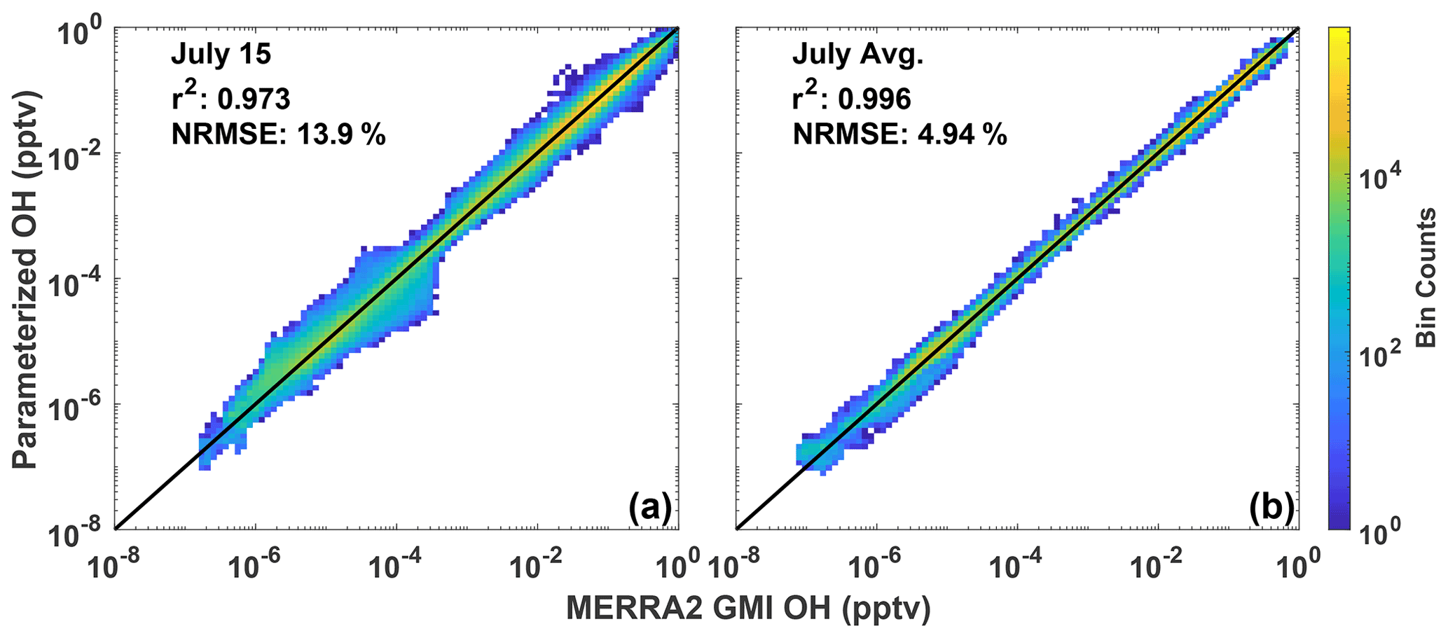
Figure 2Scatter density plot of tropospheric OH from the MERRA2 GMI simulation plotted against OH calculated by the parameterization for 15 July 2005 (a). Panel (b) shows the 24 h averaged OH output by the parameterization averaged across all July days for 2005. Colors indicate the number of data points in each bin. The r2 of a linear least-squares regression and the NRMSE are also indicated.
When we average the daily output to the monthly scale, the parameterization can reproduce the global OH distribution with little error (Figs. 1–2). For July 2005, the percentage difference between the parameterized OH and output from the MERRA2 GMI simulation in the LFT (Fig. 1b) and throughout the troposphere (Fig. S3) is generally within 10 %, outside of the Southern Hemispheric high latitudes, where it is polar night and OH concentrations are negligible. The random errors evident in the daily data in Fig. 1a average out on the monthly timescale, resulting in a tight correlation (r2=0.996) and a NRMSE of 4.94 % for all tropospheric values (Fig. 2b). Similar results are found for the July model when applied to other years (Table S1) and for parameterizations developed for other months (Figs. S3 and S4). Averaging the daily output over the monthly period yields a better NRMSE by more than a factor of 2 over climatology (NRMSE = 11 %), defined as the mean OH from the MERRA2 GMI simulation averaged over 1980 to 2019.
In regions where global CO and CH4 loss are most important, parameterization biases and errors are low. For CO and CH4, tropospheric loss to OH maximizes in the LFT in the 0–30∘ latitude band of the summer hemisphere with near-negligible loss in the winter hemisphere polar region (Fig. 3). The comparatively large overestimates and underestimates over Antarctica evident in Fig. 1 are irrelevant to the OH–CO–CH4 cycle because of the low loss rate in this region. In contrast, in regions where CO and CH4 loss maximize, the parameterization is biased low by only −0.3 % to −1.4 %. The normalized absolute error varies between 2.2 % and 4.6 % in the tropics and Northern Hemispheric midlatitudes for all tropospheric layers (MFT: pressures between 500 and 300 hPa; UFT: pressures between 300 hPa and the tropopause). Results are similar for other months.
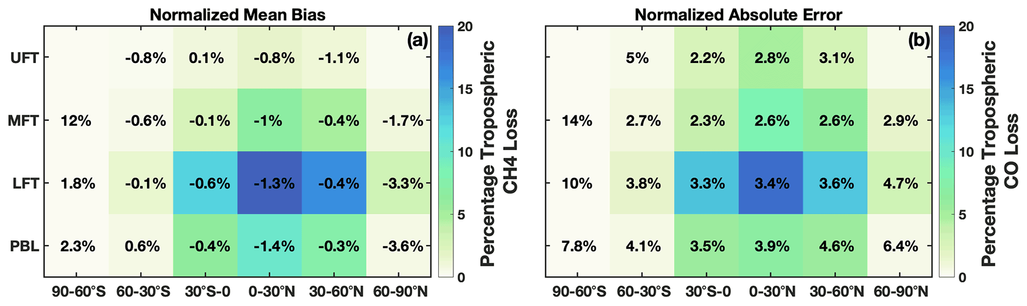
Figure 3(a) Percentage of total tropospheric CH4 lost to reaction with OH for July 2005 averaged over 30∘ zonal mean bins and four atmospheric layers is shown by the background colors. The percentage loss values account for the mass of each region relative to the total atmospheric mass. Percentages indicate the normalized mean bias of the parameterization with respect to the MERRA2 GMI simulation. Statistics for the polar UFT are omitted because low tropopause heights limit the data amount in these regions. Panel (b) is the same as panel (a) except it is for tropospheric CO loss and the normalized absolute error.
The parameterization is also able to reproduce global mean metrics of OH, such as , within 1.3 % on average. For each month of 2005, we calculated the global, mean mass-weighted tropospheric OH as described in Lawrence et al. (2001) and the mean tropospheric with respect to OH as described in Nicely et al. (2020) for the MERRA2 GMI simulation, the parameterization, and the climatological mean, defined as the average value from the MERRA2 GMI simulation between 1980 and 2019. Results for are shown in Fig. 4 and for mass-weighted OH in Fig. S5. The parameterization captures the seasonality of the , with a minimum in boreal summer and a maximum in boreal winter. Agreement varies slightly by month, differing by only 0.8 % in January and up to 2.5 % in August, although the bias is systematically low for 2005 and the other validation years (Table S1). These values are reasonable and much smaller than the inter-model variability often seen in model intercomparison projects (e.g., Nicely et al., 2020; Voulgarakis et al., 2013). Similar results are found for the global mean mass-weighted OH. The Northern Hemispheric/Southern Hemispheric OH ratio (Fig. S5) also generally agrees within 0.5 % for all months, again with the exception of August. The comparatively weaker performance for August is limited to 2005, however, as performance of the August parameterization in the other validation years (1985, 1995, and 2015) is closer to the 1 % difference shown by the parameterizations for the other months. The parameterizations present a significant improvement over the climatological mean, which for 2005 consistently underestimates for all months and by up to 6 % in March.
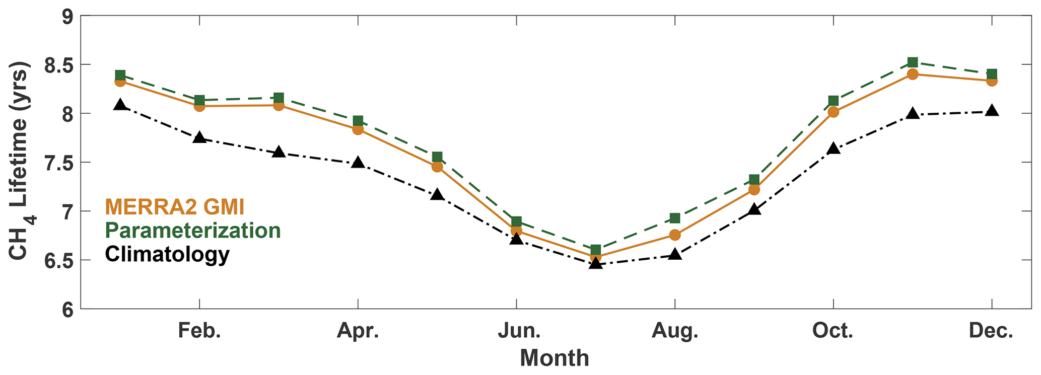
Figure 4Global mean methane lifetime with respect to tropospheric OH from the parameterization (green squares) and MERRA2 GMI (orange circles) for 2005 and the climatological average (black triangles) calculated from MERRA2 GMI for 1980–2019.
3.2 Understanding the relative importance of input parameters
While we have demonstrated that the parameterization is able to reproduce OH accurately, it is also instructive to understand the relative importance the parameterization places on each of the inputs. Although this parameterization is not a process-based example, understanding how the parameterization responds to different inputs can help determine if the regression tree is responding in a way consistent with current understanding of OH chemistry, although there are limitations to the information that can be gleaned from these metrics. We evaluate the regression tree parameterization using two metrics, the Gain feature importance as output by the XGBoost package, and SHAP values.
3.2.1 Investigating the Gain feature importance
The Gain feature importance (Chen and Guestrin, 2016) is a measure of the improvement in model accuracy achieved from adding branches in the model corresponding to a specific input variable. The Gain value therefore indicates the relative importance of each input for the model as a whole but not for individual data points. The Gain values for each input for the January and July models are shown in Fig. 5. While there are differences between the 2 months, several features are similar. Variables that indicate geographic location (e.g., SZA, latitude, and pressure) and chemical species that have previously shown to be dominant drivers of OH variability (e.g., NO2, O3, CO) and/or OH proxies (e.g., HCHO) (Wolfe et al., 2019; Murray et al., 2021) have some of the highest Gain values. As we show below, caution should be used in extrapolating results from the Gain values to a process-based understanding of OH without prior knowledge of its response to chemical and dynamical drivers.
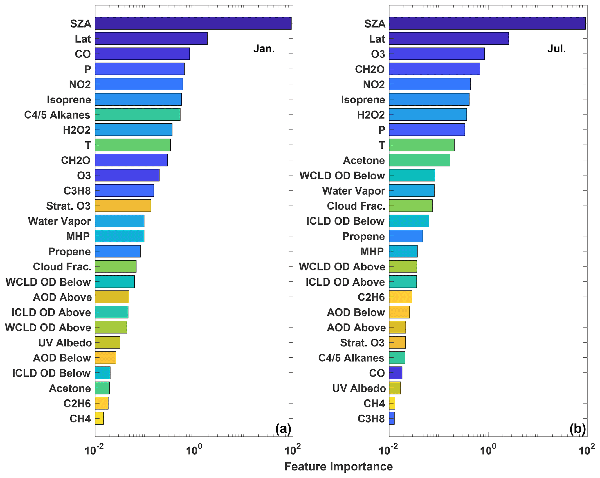
Figure 5The feature importance (gains) of the January (a) and July (b) parameterizations as calculated by XGBoost. Variables are sorted by their relative importance. WCLD stands for water cloud, ICLD stands for ice cloud, and OD stands for optical depth. “Above” and “below” for the optical depth variables indicate the optical depth above and below a particular model grid box. Colors are assigned to the variables to permit easier comparison of the panels.
The relative importance of variables that indicate location is consistent with OH chemistry and previous parameterization studies. Primary OH production is driven by the photolysis of O3 followed by the subsequent reaction of the O1D radical, produced from that photolysis, with water vapor (e.g., Spivakovsky et al., 2000). Thus, the OH distribution is strongly dependent on SZA, latitude, and pressure. This is consistent with the parameterization, where SZA and latitude have the highest Gain values for both months examined here, as well as with the results of Duncan et al. (2000), who highlighted the importance of latitude in their parameterization.
Similarly, the chemical species that are most important for controlling OH distribution on the global scale also tend to have higher Gain values. As discussed above, O3 and NOx chemistry is instrumental in controlling primary and secondary OH production on global scales (e.g., Spivakovsky et al., 2000; Anderson et al., 2021), consistent with their comparatively high Gain values. HCHO, an oxidation product of the reaction of OH with many VOCs, has been found to be a suitable proxy for OH in the remote atmosphere (Wolfe et al., 2019), consistent with its relative importance in both the July and January models.
The relative importance of global OH sinks in the parameterization, however, demonstrates the limitations of using the Gains values to interpret the regression tree model in a process-based way. CO, the dominant OH sink on a global scale (Spivakovsky et al., 2000), is the most important chemical input for the January parameterization, although it is relatively unimportant in the parameterizations for all other months. While tropical CO variability in MERRA2 GMI and biomass burning emissions (Duncan, 2003b) are larger in boreal winter than July, there is no process-based explanation for why CO should be different in January from December or February. Differences in the relative importance of CO between the 2 months does not imply that OH sensitivity to CO in MERRA2 GMI or the atmosphere varies in the same manner. Instead, the differences simply indicate that the parameterization algorithm finds CO to be more useful in predicting OH in January than July. Similarly, CH4, the second-most-important OH sink on the global scale, has low Gain values, suggesting it has little impact on model performance. This is likely because, in the MERRA2 GMI simulation, CH4 concentrations vary little within a given latitude band due to CH4 surface concentrations being set as a boundary condition. The methane distribution therefore provides little additional information beyond that already contained in the variables that indicate location.
3.2.2 Investigating parameterization SHAP values
While the Gain values indicate the relative importance of species in the parameterization and can provide some information as to whether the parameterization behaves in a manner consistent with our understanding of OH chemistry, the metric only provides information about the dataset as a whole. Gain values can therefore obscure the importance of variables that only strongly impact the parameterization for a small subset of the data. To better understand the relative importance of variables as well as the spatial variability in that importance, we also calculate the SHAP values (Lundberg and Lee, 2017), which provide information on the relative importance of each data point input into the model.
In the context of machine learning, Shapley values, an idea first developed for game theory (Shapley, 1953), indicate the average contribution of an individual model input to all possible combinations of inputs. For example, to calculate the Shapley value of the variable X for a hypothetical machine learning model with three input variables X, Y, and Z, first a model would be trained with all three variables. A new model would then be retrained, omitting X, and the difference between the two models would be calculated to determine the contribution of X. This process would then be repeated with different permutations of input variables (e.g., X and Y, X and Z) to determine the contribution of X in those instances. The final Shapley value is the average of the contribution from these different models. SHAP values use the same concept but in a manner that reduces the computation time (Lundberg and Lee, 2017), as this process could become prohibitive for a model, such as the parameterization of OH, that contains 27 inputs.
We calculate SHAP values using the TreeExplainer API of the SHAP package available for Python. One limitation of the algorithm used to calculate SHAP values is that it is too computationally expensive to calculate the SHAP values for the tuned regression tree model. Computational time to calculate SHAP values for the troposphere at the native model resolution for 1 d is several months. Maximizing computational speed by degrading the model resolution and running the SHAP package with GPUs would take approximately 4 d for one model day. Calculating SHAP values for a model with default model hyperparameters, however, takes minutes. This is due to the large reduction in the number of trees (100 to 10) and the maximum tree depth (18 to 6) in the parameterization, which significantly speeds up the creation of new regression trees needed in the SHAP value calculation.
We first evaluate the feasibility of using the SHAP values for the untuned model to explain the parameterization behavior. To test this, we created a subset of 5000 OH values from the parameterization training dataset that spanned the full range of OH concentrations. We then calculated the SHAP values for the July parameterization with tuned hyperparameters and for a July parameterization using the default XGBoost hyperparameters. For the variables found to be most important for the parameterization (e.g., SZA, NO2, O3, isoprene, HCHO, latitude), there are strong correlations (r2 of 0.97 or higher) for the SHAP values between the tuned and untuned model, resulting in similar spatial distributions, although there are differences in the magnitude. For other variables, correlation is much weaker, although the relative importance of variables is similar for the tuned and untuned parameterizations. We therefore restrict our analysis primarily to variables that have highly correlated SHAP values between the tuned and untuned models and our discussion to the relative importance of the different variables.
The distribution of SHAP values for the training dataset for July demonstrates the importance of including each of the variables as inputs to the parameterization and the large variability in their relative importance. Figure 6 shows the distribution of the SHAP values for each input parameter of the approximately 3.2 million data points used to train the July parameterization. The median SHAP values (Fig. 6) show similar ordering as the Gains feature importance (Fig. 5), with variables that indicate location, as well as O3 and NO2 being the most important in both cases. When looking at the distribution of the SHAP values, however, it becomes apparent that variables that appear to be unimportant for parameterization performance in the mean (e.g., propene and CH4) can have large importance for individual data points. For example, although propene can be locally important for OH chemistry, due to its reactivity, concentrations in the remote atmosphere are low, making the species seem unimportant in the aggregate. Similar results are found for the January parameterization (Fig. S6). As discussed in Sect. 2.2, the SHAP values provide a rationale for including each of these species in the parameterization.
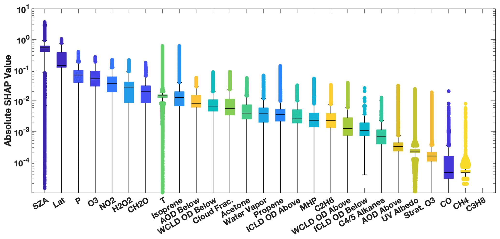
Figure 6Distribution of the absolute SHAP value for each parameterization input for July from an untuned version of the parameterization of OH. Input parameters are sorted by order of relative importance. The median is indicated with the black line, the edges of the box represent the interquartile range, and the whiskers represent the 5th and 95th percentile. Values outside this range are indicated with circles. Note that the SHAP value for propane is zero, indicating that it is not used by the untuned parameterization.
The SHAP values also demonstrate the spatial distribution of the relative importance of the different chemical OH drivers. Figure 7 shows the relative importance of NO2, as determined by the SHAP values for the untuned parameterization, for both the zonal mean and the LFT. Note that the untuned parameterization has large errors for low OH concentrations, and thus SHAP values poleward of 45∘ S should be viewed as more uncertain than those elsewhere. In both the horizontal and vertical, the SHAP values demonstrate that the parameterization captures the spatial pattern of the relative importance of NOx for OH production. The spatial pattern in Fig. 7a, for example, has the highest contribution of NO2 to the total SHAP value in the tropical UFT and in the Northern Hemisphere midlatitudes. This is nearly identical to the spatial pattern of the relative contribution of the NO + HO2 reaction to overall OH production in the MERRA2 GMI simulation (Anderson et al., 2021). Likewise, in the LFT, the contribution from NO2 maximizes over continental regions with high emission and minimizes over the remote oceans. The spatial pattern of SHAP values of isoprene also agree with OH chemistry, maximizing in regions of strong biogenic emissions and minimizing over oceans (Fig. S7). These SHAP values demonstrate that although the parameterization is not process-based, its behavior at least partially accords with our understanding of OH chemistry.
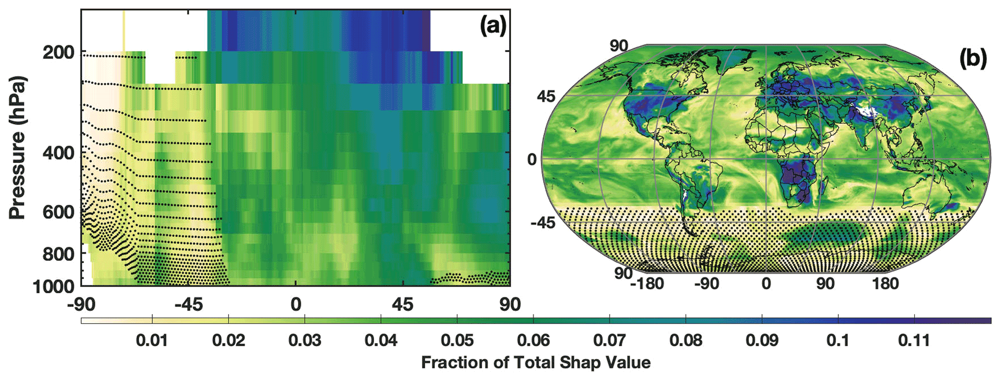
Figure 7The fraction of the contribution of the NO2 SHAP value to the sum of the absolute SHAP value of all inputs in July is shown for the zonal mean (a) and the LFT (b). Regions where mean OH mixing ratios are below 0.03 pptv, the point below which the untuned parameterization is unable to reasonably predict OH, are indicated by the stippling.
3.3 Case study: testing the parameterization response to the 2016 El Niño Event
While we have demonstrated that the parameterization can satisfactorily reproduce OH during all months of 2005, we now investigate its ability to capture OH accurately during the 2016 El Niño event that we excluded from the training dataset. Evaluating how the parameterization responds to deviations from the climatological mean of the inputs during a large-scale event on which it was not trained, such as the 2016 El Niño, is a strong test of its ability to predict extremes in OH and to respond to deviations from the climatological mean of the parameterization inputs. The response of the parameterized OH to these extremes in inputs will also provide a further test of the ability of the parameterization to behave in a process-based way.
El Niño events lead to dramatic changes in the concentrations and distributions of many OH drivers, including O3 (Oman et al., 2011, 2013), CO (Duncan, 2003a; Rowlinson et al., 2019), NOx (Murray et al., 2013, 2014), and water vapor (Shi et al., 2018; Anderson et al., 2021). As such, the El Niño–Southern Oscillation (ENSO) is the dominant mode of OH variability throughout much of the troposphere and can result in localized changes in OH on the order of 40 %–50 % from the climatological mean (Anderson et al., 2021; Turner et al., 2018). Changes in secondary production from NOx in the UFT and changes in primary production from O3 in the PBL and LFT drive the ENSO-related variability of OH (Anderson et al., 2021). Methane emissions also vary strongly with the ENSO phase (Zhang et al., 2018; Worden et al., 2013). In order to capture the OH–CH4–CO system correctly, the parameterization must be able to capture ENSO-related OH variability.
Here, we investigate the ability of the parameterization to capture OH during the El Niño events of 1997–1998 and 2015–2016, two of the largest such events during the period of the MERRA2 GMI simulation according to the Multivariate ENSO Index (Wolter and Timlin, 2011). The 1997–1998 event, which was included in the training dataset, was a prototypical example of an eastern Pacific (EP) El Niño, characterized by sea surface temperature (SST) anomalies extending to the coast of South America. In contrast, the 2015/2016 event was a blend of an EP and a central Pacific (CP) El Niño, also known as El Niño Modoki, where SST anomalies extend only to the international dateline (Paek et al., 2017). These different “flavors” of El Niño affect atmospheric distributions of OH drivers, such as water vapor (Du et al., 2021), in different ways, suggesting different impacts on OH. While we did include other blended El Niños (1986–1987, 1987–1988, and 1991–1992) (Kug et al., 2009) in the training dataset, each had responses in the atmospheric distribution of OH and its drivers distinct from the 2015–2016 event. We focus our investigation on January and the MFT, the time and location of the strongest correlation between ENSO and OH (Anderson et al., 2021) in the MERRA2 GMI simulation. We also restrict the analysis to the OH precursors, NO2, CO, and O3, as they have both a strong influence on the variability of ENSO-related OH production and loss and have comparatively large feature importance and SHAP values in the January parameterization.
For both the 1997–1998 and 2015–2016 El Niño events, each OH driver examined deviates strongly from the climatological mean, defined as the average value from the MERRA2 GMI simulation over all January months from 1980–2019. Both O3 and NO2 have pronounced positive anomalies over the western Pacific and Maritime Continent and negative anomalies over the eastern Pacific (Fig. 8) that extend throughout much of the free troposphere (Fig. S8), likely associated with changes in the Walker circulation as described in Oman et al. (2011). The positive anomalies over Indonesia show a distinct westward shift during the 1997–1998 event as compared to 2015–2016, highlighting the variability in the effects of ENSO on emissions and transport. CO has a large positive anomaly over much of the globe, attributable to the increases in biomass burning during El Niño events (e.g., Duncan, 2003a). As with O3 and NO2, there are large differences in the spatial pattern of the CO anomalies between the two events, particularly over the Indian Ocean, central Africa, and South America.
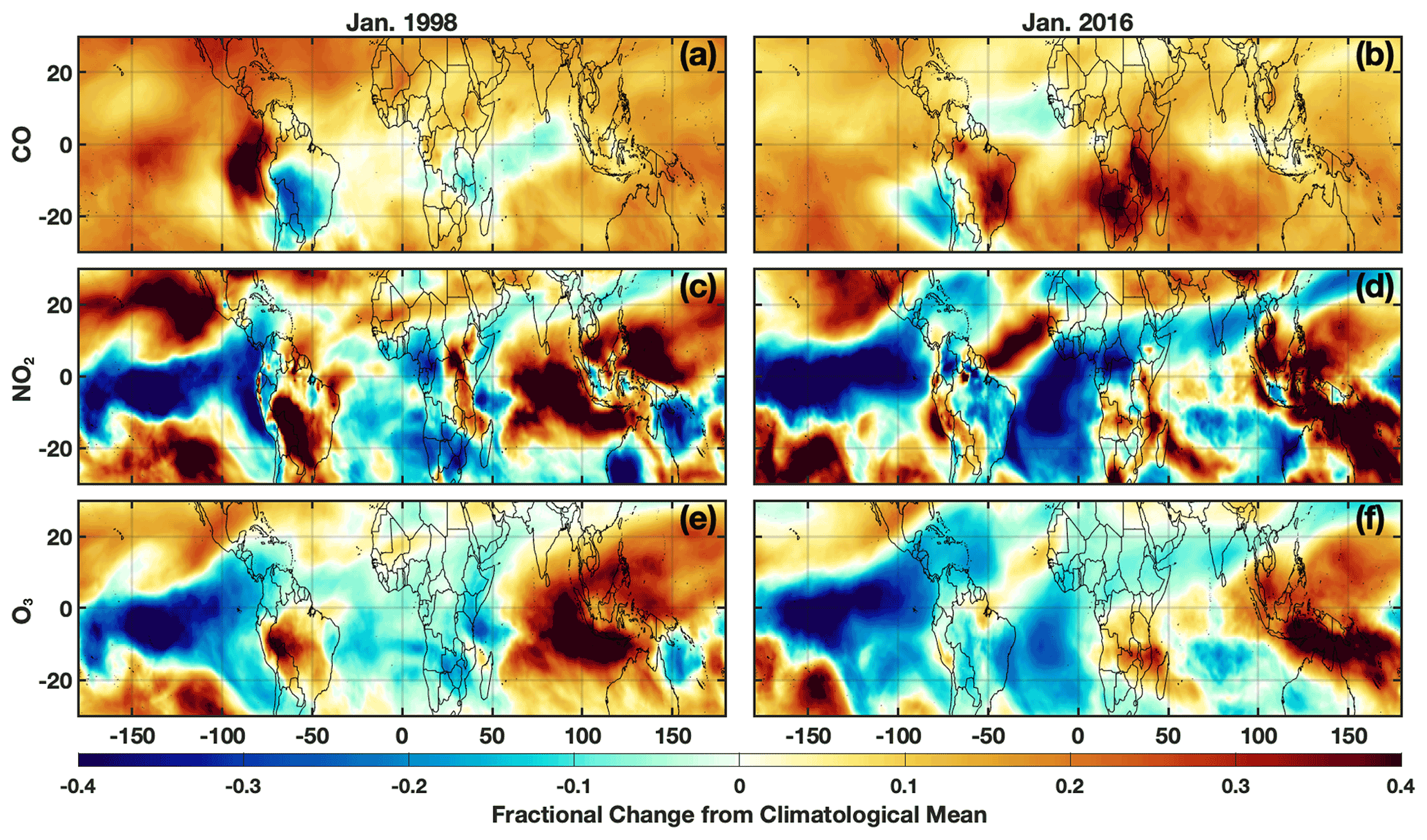
Figure 8Fractional difference in the indicated variable between January 1998 (a, c, e) and the climatological mean (1980–2019) calculated from the MERRA2 GMI simulation for the MFT. The same values but for January 2016 are indicated on the right. Species shown are CO (a, b), NO2 (c, d), and O3 (e, f).
The differences in anomalies of the OH drivers between the 1997–1998 and 2015–2016 El Niño events lead to distinct anomaly patterns in OH itself. During the 1997–1998 event, in the MFT there are noticeable positive anomalies in OH over much of the Indian Ocean basin, the southeastern Pacific, South America, and the western Atlantic Ocean (Fig. 9). During 2015–2016, the positive anomalies were more limited and most noticeable in the tropical western Pacific Ocean and southern Indian Ocean. Along the Equator, the positive anomalies extended throughout a larger portion of the troposphere during January 1998 than 2016. Both the parameterization inputs and the OH itself respond strongly and in different ways to each El Niño event, providing a strong test to determine the robustness of the parameterization.
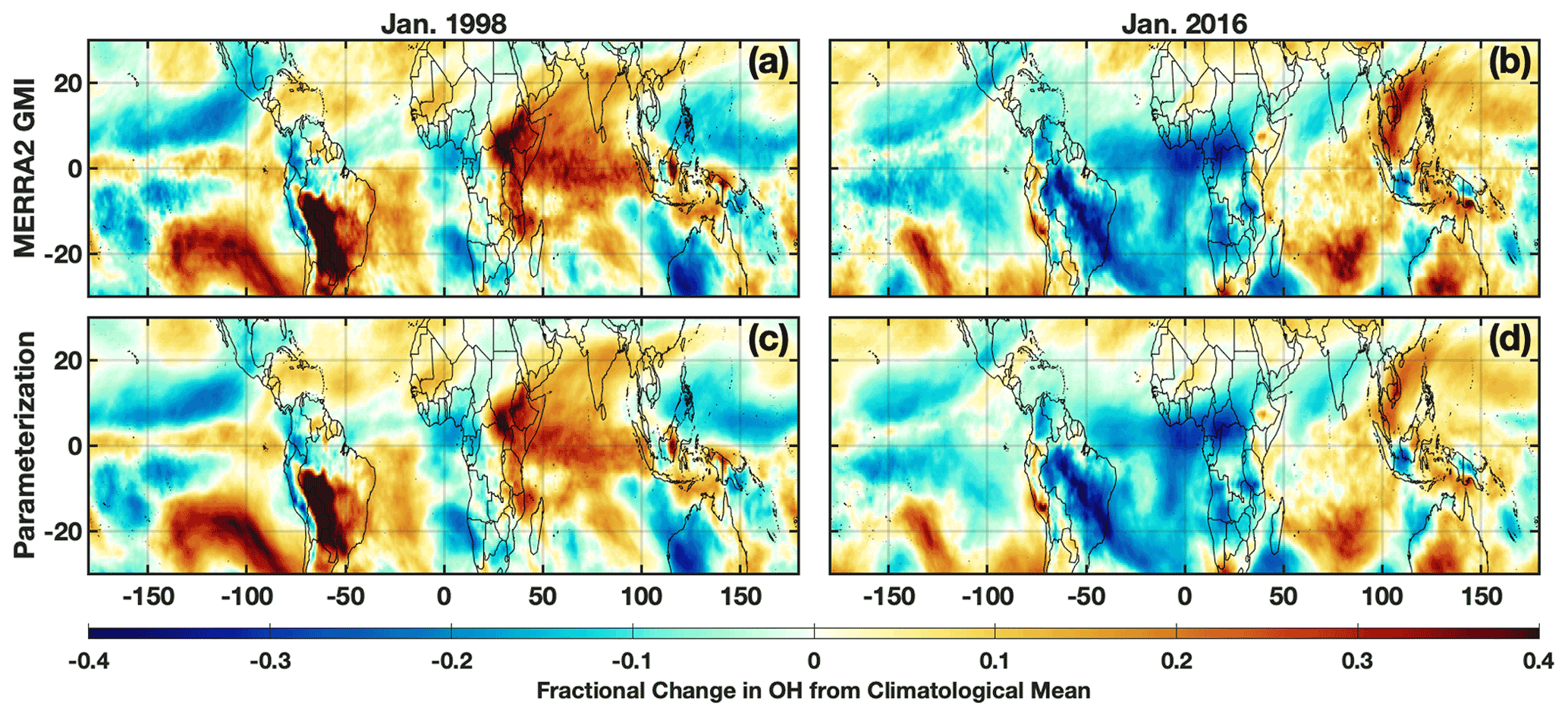
Figure 9Fractional difference in the indicated variable between January 1998 (a, c) and the climatological mean (1980–2019) calculated from the MERRA2 GMI simulation averaged over the MFT. The same values but for January 2016 are indicated on the right. Species shown are OH from the MERRA2 GMI simulation (a, b) and OH calculated by the parameterization (c, d).
The parameterization reproduces the ENSO-related OH anomalies for both El Niño events with remarkable fidelity. We ran the parameterization for all January months from 1980 to 2016 to calculate a climatology and calculated the deviations for 1998 and 2016 from that value. For both events, the parameterization accurately captures the location and magnitude, as well as the spatial pattern, of the OH anomalies with a few minor exceptions in the horizontal and vertical (Figs. 9 and S8). Correlation between the MERRA2 GMI and parameterized anomalies plotted in Fig. 9 has an r2 of 0.93 or higher for both years. The parameterization is therefore capable of reproducing both the climatological mean of OH and large deviations in the mean in response to strong climatological deviations in the model inputs, even for years excluded from the training dataset.
In this paper, we present a new methodology to generate a parameterization of OH that is efficient and easy to use compared to previous methods (e.g., Spivakovsky et al., 1990; Duncan et al., 2000), allowing the user to rapidly update the parameterization of OH as necessary. The new method uses GBRTs and a full-chemistry simulation from a CCM as the training data to generate the parameterization of OH with a high degree of accuracy relative to the full-chemistry simulation. We illustrated our methodology with a parameterization designed for the ECCOH module of the GEOS CCM.
The parameterization of OH accurately reproduces OH from the full-chemistry simulation on which it was trained, but it may not produce the desired accuracy for a given time period or scenario outside the range represented in the training data. Of course, the degree of degradation in accuracy depends on how far inputs exceed the ranges of the training dataset. In addition, the parameterization of OH generated using inputs from one model may not be portable to another model or even a different configuration of the same model as shown below. The simulated relationships between OH and the input parameters may differ because of inter-model variations in the chemical, dynamical, and radiative schemes. Ultimately, it is up to the user to determine an acceptable level of degradation for a specific research topic. In this section, we give an example of the degree of degradation in accuracy for a parameterization of OH that uses (1) a different time period for the same model and (2) input parameters from a different model.
4.1 Input parameters from a different time period for the same model setup
Analysis of a separate model simulation, the Chemistry Climate Model Initiative (CCMI) GEOS simulation (Morgenstern et al., 2017), highlights possible limitations in extending the parameterization to years outside of those on which it was trained, particularly if there is a strong trend in one of the inputs. The GEOS CCMI simulation has unconstrained meteorology, spans 1960–2100, and has a horizontal resolution of 2.0∘ latitude × 2.5∘ longitude. Emissions for precursors of tropospheric O3 and aerosols are from the RCP6.0 scenario. We trained two new parameterizations on the CCMI dataset, denoted CCMI2019 and CCMI2060, using data from 1980–2019 and 1980–2061, respectively. We used the same methodology to create the training datasets as for the MERRA2 GMI parameterization. CCMI output data are only available at monthly resolution, and thus we trained the CCMI parameterizations on monthly, instead of daily, averaged values. Every 10th year, staring in 2000, was omitted from the training dataset for validation.

Figure 10Time series showing the percent difference between calculated from the CCMI simulation and from three separate parameterizations: one trained on MERRA2 GMI output from 1980–2019 (blue circle), one trained on CCMI output spanning 1980–2019 (red triangle), and one trained on CCMI output spanning 1980–2060 (purple square). The stratospheric O3 column (orange star) from the CCMI simulation averaged over 30∘ S to 60∘ N, the region where tropospheric CH4 loss to OH maximizes (Fig. 3), is also shown. All data are for July.
While the CCMI2019 parameterization performed similarly to the MERRA2 GMI parameterization for years included in the training dataset, performance degraded significantly for years beyond 2019. The CCMI2019 parameterization captured the for 2000 and 2010 within 1 % (Fig. 10, red line) and the NRMSE within 5 % (not shown). When we applied the parameterization to years outside of the training window, however, performance degraded quickly and by 2060 underestimated by about 4 %. The CCMI2060 parameterization, on the other hand, captures the lifetime within 0.5 % for all validation years.
The reason for this performance degradation is likely due to input parameters that extend beyond the range used in the training dataset. For example, there is a strong positive trend in the stratospheric O3 column (Fig. 10), which results in chemical environments in 2060 that did not exist in the 1980–2019 training dataset. Other variables with strong trends, such as CH4 and temperature, as well as different large-scale dynamical patterns, could also decrease parameterization performance. These results strongly suggest caution when applying the parameterization to future scenarios outside of the training window. As will be discussed in the following section, care should be taken in choosing the training dataset to ensure that it represents the full range of photochemical conditions on which the parameterization will be applied.
4.2 Input parameters from a different model setup
Similar to applying the parameterization outside of the time frame on which it was trained, applying the parameterization to a different model setup also warrants caution, as the differences can result in new chemical environments on which the parameterization was not trained. We now discuss parameterization performance when output from the CCMI simulation discussed in Sect. 4.1 is input into the MERRA2 GMI-trained parameterization. Despite both simulations being from the GEOS framework, the CCMI simulation setup differs from the MERRA2 GMI simulation in emissions, time frame, resolution, and meteorology (unconstrained vs. specified dynamics), among other factors. Because CCMI output is only available at a monthly resolution, we created a separate parameterization, hereafter referred to as “M2GMI-monthly”, using MERRA2 GMI output with identical parameterization inputs as the daily parameterization but using monthly averaged values. Performance is similar to that of the parameterization trained on daily data and averaged over monthly timescales, with the NRMSE for the troposphere on the order of 6 %–7 % depending on the year.
When output from the CCMI simulation is used as inputs to the M2GMI-monthly parameterization, performance degrades significantly. For July 2000, for example, there are distinct regions of both positive and negative biases (Fig. 11a) in parameterized OH, resulting in a NRMSE of 13 %, on par with using climatology as an OH estimate. Because the largest discrepancies are centered outside of the tropics and/or in regions with low concentrations, for year 2000 is identical between the CCMI and parameterized OH. When applied to 2060 (Fig. 11c), which is far outside the training period of the M2GMI-monthly parameterization, there is a near universal high bias in parameterized OH, resulting in a NRMSE of 16 % and a biased low by 4.5 %. This overestimate results in a negative trend in from parameterized OH from 2000 to 2060 (Fig. 10, blue line), despite the trend in the CCMI simulation being positive. Applying the MERRA2 GMI parameterization to a study using the CCMI setup would therefore misrepresent the OH–CH4 cycle.
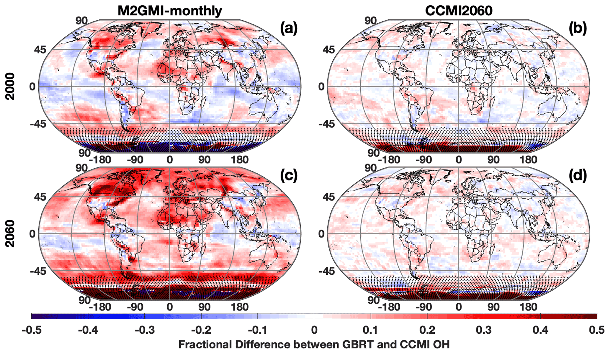
Figure 11Fractional difference between OH calculated by the M2GMI-monthly (a, c) and the CCMI2060 (b, d) parameterizations and OH output from the CCMI simulation. Data are averaged between 850 and 500 hPa for July 2000 (a, b) and July 2060 (c, d). Regions with low OH, defined as a mixing ratio of less than 0.005 pptv, are indicated with stippling.
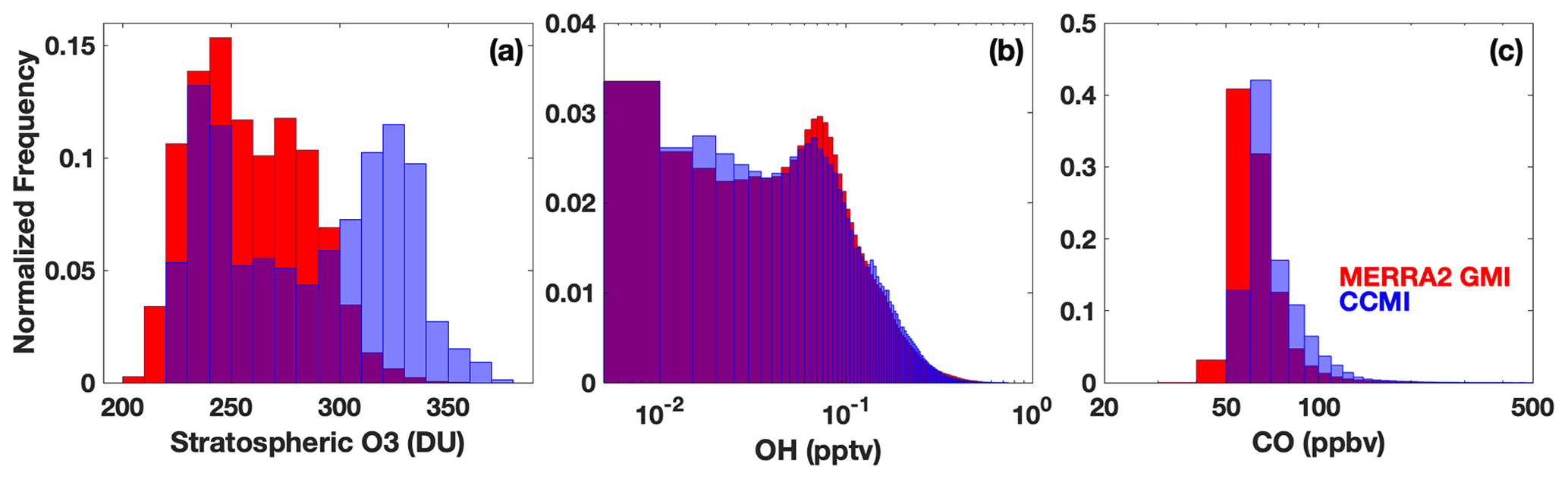
Figure 12Histograms showing the distribution of stratospheric column O3 (a), tropospheric OH (b), and tropospheric CO (c) from the M2GMI-monthly parameterization training dataset (red) and from the CCMI simulation for 2060 (blue). Purple indicates areas of overlap between the two distributions.
Through an analysis of the ranges of input parameters from both simulations, we found that the differences in parameterization performance for inputs from MERRA2 GMI and CCMI are likely largely attributable to differences in the stratospheric O3 distributions between the two simulations. In 2060, for example, CCMI stratospheric O3 has a much higher frequency of values above 300 DU than the M2GMI-monthly training dataset (Fig. 12). A smaller, but still noticeable, shift in the distribution is also found for the year 2000 (Fig. S9). Likewise, the accuracy of the M2GMI-monthly parameterization decreases from 2000–2060 as the stratospheric O3 burden increases (Fig. 10, red line). Mechanistically, higher stratospheric ozone in CCMI should result in lower tropospheric OH because the reduction in incoming ultraviolet radiation limits tropospheric O3 photolysis. This could also lead to a higher CO burden, due to the smaller OH sink. Comparisons between the OH and CO distributions from the two simulations are consistent with this hypothesis. Even though the M2GMI-monthly training dataset spanned the full range of stratospheric O3 values from the CCMI simulation, the frequency of stratospheric O3 values at higher concentrations likely creates chemical environments in the CCMI simulation distinct from those in MERRA2 GMI, forcing the parameterization to extrapolate to a chemical space on which it was not trained. This highlights the need to compare the distribution of any parameterization inputs to that of the training dataset to ensure that the training dataset fully encompasses the range of photochemical environments necessary for a given study. Once integrated into a modeling framework, safeguards could be added to warn a user if parameterization input values fall outside of the bounds of the training dataset, as is done with the current ECCOH parameterization.
Again, performance improves significantly when we apply output from the CCMI simulation to the CCMI2060 parameterization. The regions of consistent high bias notable when CCMI output was applied to the M2GMI-monthly parameterization are absent for both 2000 and 2060, and NRMSE shows a factor of 3 improvement over the previously discussed scenario. Likewise, for all validation years, the parameterized OH resulted in a that agreed with the CCMI simulation between 0 % and −0.46 % (purple line, Fig. 10).
We conclude that for best performance a separate parameterization should be created for each new modeling framework to capture OH variability accurately. This will not create an undue computational expense on an experiment. Because a full-chemistry simulation is necessary to create the parameterization inputs of chemical species that are not calculated online, the necessary data to create a training dataset will already be available. The only additional time will be that required to format the regression tree inputs and to train the model, which takes approximately 2–3 h for each month. This process can be performed using previously created Python scripts with minimal changes. The flexibility that this modeling framework permits will facilitate its use even if there are major changes to the underlying model chemistry or dynamics.
The methodology we present here allows for the quick generation of a parameterization of OH for use in a chemistry–climate model to help disentangle the complicated relationship between CO, CH4, and OH. The parameterization is designed for computationally inexpensive sensitivity runs and, as such, is not designed to capture feedbacks between OH and all of its chemical and dynamical drivers (e.g., H2O2 or MHP). Instead, if a user is interested in these feedbacks, they could use the results of the sensitivity tests to identify times, locations, or chemical regimes for a targeted full-chemistry simulation. Likewise, the parameterization reflects the photochemical environments of the dataset on which it was trained. Therefore, the training dataset should be carefully chosen to reflect the goals of a given study. However, we have demonstrated that the sample parameterization outlined here accurately predicts the magnitude and spatial distribution of the large deviations in OH for the 2016 El Niño, an event that was not part of the training dataset. This result gives confidence in the fidelity of a parameterization developed with our methodology when simulating the spatial and temporal responses of OH to perturbations from large variations in the chemical, dynamical, and solar irradiance drivers of OH.
The scripts used to create the training datasets and a sample script to create a parameterization have been archived by Zenodo at https://doi.org/10.5281/zenodo.6046037 (Anderson, 2022a). A sample parameterization for the ECCOH module trained on MERRA2-GMI output is available at https://doi.org/10.5281/zenodo.6604130 (Anderson, 2022b).
Output from the MERRA2 GMI simulation are publicly available at https://acd-ext.gsfc.nasa.gov/Projects/GEOSCCM/MERRA2GMI/ (NASA Goddard Space Flight Center, 2022). The training dataset and training targets for the July parameterization presented here are available at https://doi.org/10.5281/zenodo.6604130 (Anderson, 2022b). Output from the GEOSCCM simulation for CCMI is available at the Centre for Environmental Data Analysis (CED), the Natural Environment Research Council's Data Repository for Atmospheric Science and Earth Observation, at http://data.ceda.ac.uk/badc/wcrp-ccmi/data/CCMI-1/output (CEDA Archive, 2022).
The supplement related to this article is available online at: https://doi.org/10.5194/gmd-15-6341-2022-supplement.
DCA wrote the manuscript, performed the data analysis, and created the parameterizations. BND and MBFC developed the idea for the parameterization. SAS performed three-dimensional modeling for the work. JMN and PDI provided advice on machine learning. JL helped perform data analysis. All authors helped develop ideas for the analysis and contributed to the manuscript.
The contact author has declared that none of the authors has any competing interests.
Publisher's note: Copernicus Publications remains neutral with regard to jurisdictional claims in published maps and institutional affiliations.
This research has been supported by the National Aeronautics and Space Administration (NASA) Modeling, Analysis, and Prediction (MAP) program (grant no. 80NSSC17K0220). In addition, the authors received funding from the NASA Aura program.
This paper was edited by Fiona O'Connor and reviewed by two anonymous referees.
Anderson, D. C., Duncan, B. N., Fiore, A. M., Baublitz, C. B., Follette-Cook, M. B., Nicely, J. M., and Wolfe, G. M.: Spatial and temporal variability in the hydroxyl (OH) radical: understanding the role of large-scale climate features and their influence on OH through its dynamical and photochemical drivers, Atmos. Chem. Phys., 21, 6481–6508, https://doi.org/10.5194/acp-21-6481-2021, 2021.
Anderson, D. C., Follette-Cook, M. B., Strode, S. A., Nicely, J. M., Liu, J., Ivatt, P. D., and Duncan, B. N.: Code for the development of a parameterization of OH for CCMs, Zenodo [code], https://doi.org/10.5281/zenodo.6046037, 2022a.
Anderson, D. C., Follette-Cook, M. B., Strode, S. A., Nicely, J .M., Liu, J., Ivatt, P. D., and Duncan, B. N.: Sample ECCOH OH Parameterization (1.0), Zenodo [code and data set], https://doi.org/10.5281/zenodo.6604130, 2022b.
CEDA Archive: CCMI-1 Data Archive, CEDA Archive [data set], http://data.ceda.ac.uk/badc/wcrp-ccmi/data/CCMI-1/output, last access: 4 Aug. 2022.
Chen, T. and Guestrin, C.: XGBoost: A Scalable Tree Boosting System, KDD '16: Proceedings of the 22nd ACM SIGKDD International Conference on Knowledge Discovery and Data Mining, San Francisco, CA, USA, 13–17 August 2016, 785–794, https://doi.org/10.1145/2939672.2939785, 2016.
Chen, Y.-H. and Prinn, R. G.: Estimation of atmospheric methane emissions between 1996 and 2001 using a three-dimensional global chemical transport model, J. Geophys. Res.-Atmos., 111, D10307, https://doi.org/10.1029/2005JD006058, 2006.
Chin, M., Ginoux, P., Kinne, S., Torres, O., Holben, B. N., Duncan, B. N., Martin, R. V., Logan, J. A., Higurashi, A., and Nakajima, T.: Tropospheric Aerosol Optical Thickness from the GOCART Model and Comparisons with Satellite and Sun Photometer Measurements, J. Atmos. Sci., 59, 461–483, https://doi.org/10.1175/1520-0469(2002)059<0461:TAOTFT>2.0.CO;2, 2002.
Colarco, P., da Silva, A., Chin, M., and Diehl, T.: Online simulations of global aerosol distributions in the NASA GEOS-4 model and comparisons to satellite and ground-based aerosol optical depth, J. Geophys. Res.-Atmos., 115, D14207, https://doi.org/10.1029/2009JD012820, 2010.
Du, M., Huang, K., Zhang, S., Huang, C., Gong, Y., and Yi, F.: Water vapor anomaly over the tropical western Pacific in El Niño winters from radiosonde and satellite observations and ERA5 reanalysis data, Atmos. Chem. Phys., 21, 13553–13569, https://doi.org/10.5194/acp-21-13553-2021, 2021.
Duncan, B., Portman, D., Bey, I., and Spivakovsky, C.: Parameterization of OH for efficient computation in chemical tracer models, J. Geophys. Res.-Atmos., 105, 12259–12262, https://doi.org/10.1029/1999JD901141, 2000.
Duncan, B. N.: Indonesian wildfires of 1997: Impact on tropospheric chemistry, J. Geophys. Res., 108, D154458, https://doi.org/10.1029/2002jd003195, 2003a.
Duncan, B. N.: Interannual and seasonal variability of biomass burning emissions constrained by satellite observations, J. Geophys. Res., 108, D24100, https://doi.org/10.1029/2002jd002378, 2003b.
Duncan, B. N. and Logan, J. A.: Model analysis of the factors regulating the trends and variability of carbon monoxide between 1988 and 1997, Atmos. Chem. Phys., 8, 7389–7403, https://doi.org/10.5194/acp-8-7389-2008, 2008.
Duncan, B. N., Logan, J. A., Bey, I., Megretskaia, I. A., Yantosca, R. M., Novelli, P. C., Jones, N. B., and Rinsland, C. P.: Global budget of CO, 1988–1997: Source estimates and validation with a global model, J. Geophys. Res., 112, D22301, https://doi.org/10.1029/2007jd008459, 2007a.
Duncan, B. N., Strahan, S. E., Yoshida, Y., Steenrod, S. D., and Livesey, N.: Model study of the cross-tropopause transport of biomass burning pollution, Atmos. Chem. Phys., 7, 3713–3736, https://doi.org/10.5194/acp-7-3713-2007, 2007b.
Elith, J., Leathwick, J. R., and Hastie, T.: A working guide to boosted regression trees, J. Anim. Ecol., 77, 802–813, https://doi.org/10.1111/j.1365-2656.2008.01390.x, 2008.
Elshorbany, Y. F., Duncan, B. N., Strode, S. A., Wang, J. S., and Kouatchou, J.: The description and validation of the computationally Efficient CH4–CO–OH (ECCOHv1.01) chemistry module for 3-D model applications, Geosci. Model Dev., 9, 799–822, https://doi.org/10.5194/gmd-9-799-2016, 2016.
Fiore, A. M., Horowitz, L. W., Dlugokencky, E. J., and West, J. J.: Impact of meteorology and emissions on methane trends, 1990–2004, Geophys. Res. Lett., 33, L12809, https://doi.org/10.1029/2006gl026199, 2006.
Gaubert, B., Worden, H. M., Arellano, A. F. J., Emmons, L. K., Tilmes, S., Barré, J., Martinez Alonso, S., Vitt, F., Anderson, J. L., Alkemade, F., Houweling, S., and Edwards, D. P.: Chemical Feedback From Decreasing Carbon Monoxide Emissions, Geophys. Res. Lett., 44, 9985–9995, https://doi.org/10.1002/2017GL074987, 2017.
Gelaro, R., McCarty, W., Suarez, M. J., Todling, R., Molod, A., Takacs, L., Randles, C., Darmenov, A., Bosilovich, M. G., Reichle, R., Wargan, K., Coy, L., Cullather, R., Draper, C., Akella, S., Buchard, V., Conaty, A., da Silva, A., Gu, W., Kim, G. K., Koster, R., Lucchesi, R., Merkova, D., Nielsen, J. E., Partyka, G., Pawson, S., Putman, W., Rienecker, M., Schubert, S. D., Sienkiewicz, M., and Zhao, B.: The Modern-Era Retrospective Analysis for Research and Applications, Version 2 (MERRA-2), J. Climate, 30, 5419–5454, https://doi.org/10.1175/JCLI-D-16-0758.1, 2017.
Holmes, C. D.: Methane Feedback on Atmospheric Chemistry: Methods, Models, and Mechanisms, J. Adv. Model. Earth Sy., 10, 1087–1099, https://doi.org/10.1002/2017MS001196, 2018.
Ivatt, P. D. and Evans, M. J.: Improving the prediction of an atmospheric chemistry transport model using gradient-boosted regression trees, Atmos. Chem. Phys., 20, 8063–8082, https://doi.org/10.5194/acp-20-8063-2020, 2020.
Keller, C. A. and Evans, M. J.: Application of random forest regression to the calculation of gas-phase chemistry within the GEOS-Chem chemistry model v10, Geosci. Model Dev., 12, 1209–1225, https://doi.org/10.5194/gmd-12-1209-2019, 2019.
Kelp, M. M., Jacob, D. J., Kutz, J. N., Marshall, J. D., and Tessum, C. W.: Toward Stable, General Machine-Learned Models of the Atmospheric Chemical System, J. Geophys. Res.-Atmos., 125, e2020JD032759, https://doi.org/10.1029/2020JD032759, 2020.
Kleipool, Q. L., Dobber, M. R., de Haan, J. F., and Levelt, P. F.: Earth surface reflectance climatology from 3 years of OMI data, J. Geophys. Res.-Atmos., 113, D18308, https://doi.org/10.1029/2008JD010290, 2008.
Kug, J.-S., Jin, F.-F., and An, S.-I.: Two Types of El Niño Events: Cold Tongue El Niño and Warm Pool El Niño, J. Climate, 22, 1499–1515, https://doi.org/10.1175/2008JCLI2624.1, 2009.
Laughner, J. L., Neu, J. L., Schimel, D., Wennberg, P. O., Barsanti, K., Bowman, K. W., Chatterjee, A., Croes, B. E., Fitzmaurice, H. L., Henze, D. K., Kim, J., Kort, E. A., Liu, Z., Miyazaki, K., Turner, A. J., Anenberg, S., Avise, J., Cao, H., Crisp, D., de Gouw, J., Eldering, A., Fyfe, J. C., Goldberg, D. L., Gurney, K. R., Hasheminassab, S., Hopkins, F., Ivey, C. E., Jones, D. B. A., Liu, J., Lovenduski, N. S., Martin, R. V., McKinley, G. A., Ott, L., Poulter, B., Ru, M., Sander, S. P., Swart, N., Yung, Y. L., and Zeng, Z. C.: Societal shifts due to COVID-19 reveal large-scale complexities and feedbacks between atmospheric chemistry and climate change, P. Natl. Acad. Sci. USA, 118, e210948118, https://doi.org/10.1073/pnas.2109481118, 2021.
Lawrence, M. G., Jöckel, P., and von Kuhlmann, R.: What does the global mean OH concentration tell us?, Atmos. Chem. Phys., 1, 37–49, https://doi.org/10.5194/acp-1-37-2001, 2001.
Lundberg, S. M. and Lee, S.-I.: A Unified Approach to Interpreting Model Predictions, NeurIPS Proceedings, Adv. Neural In., 30, 4765–4774, 2017.
Morgenstern, O., Hegglin, M. I., Rozanov, E., O'Connor, F. M., Abraham, N. L., Akiyoshi, H., Archibald, A. T., Bekki, S., Butchart, N., Chipperfield, M. P., Deushi, M., Dhomse, S. S., Garcia, R. R., Hardiman, S. C., Horowitz, L. W., Jöckel, P., Josse, B., Kinnison, D., Lin, M., Mancini, E., Manyin, M. E., Marchand, M., Marécal, V., Michou, M., Oman, L. D., Pitari, G., Plummer, D. A., Revell, L. E., Saint-Martin, D., Schofield, R., Stenke, A., Stone, K., Sudo, K., Tanaka, T. Y., Tilmes, S., Yamashita, Y., Yoshida, K., and Zeng, G.: Review of the global models used within phase 1 of the Chemistry–Climate Model Initiative (CCMI), Geosci. Model Dev., 10, 639–671, https://doi.org/10.5194/gmd-10-639-2017, 2017.
Murray, L. T., Logan, J. A., and Jacob, D. J.: Interannual variability in tropical tropospheric ozone and OH: The role of lightning, J. Geophys. Res.-Atmos., 118, 11468–11480, https://doi.org/10.1002/jgrd.50857, 2013.
Murray, L. T., Mickley, L. J., Kaplan, J. O., Sofen, E. D., Pfeiffer, M., and Alexander, B.: Factors controlling variability in the oxidative capacity of the troposphere since the Last Glacial Maximum, Atmos. Chem. Phys., 14, 3589–3622, https://doi.org/10.5194/acp-14-3589-2014, 2014.
Murray, L. T., Fiore, A. M., Shindell, D. T., Naik, V., and Horowitz, L. W.: Large uncertainties in global hydroxyl projections tied to fate of reactive nitrogen and carbon, P. Natl. Acad. Sci. USA, 118, e2115204118, https://doi.org/10.1073/pnas.2115204118, 2021.
NASA Goddard Space Flight Center: MERRA2 GMI, NASA [data set], https://acd-ext.gsfc.nasa.gov/Projects/GEOSCCM/MERRA2GMI/, last access: 4 August 2022.
Nicely, J. M., Salawitch, R. J., Canty, T., Anderson, D. C., Arnold, S. R., Chipperfield, M. P., Emmons, L. K., Flemming, J., Huijnen, V., Kinnison, D. E., Lamarque, J.-F., Mao, J., Monks, S. A., Steenrod, S. D., Tilmes, S., and Turquety, S.: Quantifying the causes of differences in tropospheric OH within global models, J. Geophys. Res.-Atmos., 122, 1983–2007, https://doi.org/10.1002/2016JD026239, 2017.
Nicely, J. M., Duncan, B. N., Hanisco, T. F., Wolfe, G. M., Salawitch, R. J., Deushi, M., Haslerud, A. S., Jöckel, P., Josse, B., Kinnison, D. E., Klekociuk, A., Manyin, M. E., Marécal, V., Morgenstern, O., Murray, L. T., Myhre, G., Oman, L. D., Pitari, G., Pozzer, A., Quaglia, I., Revell, L. E., Rozanov, E., Stenke, A., Stone, K., Strahan, S., Tilmes, S., Tost, H., Westervelt, D. M., and Zeng, G.: A machine learning examination of hydroxyl radical differences among model simulations for CCMI-1, Atmos. Chem. Phys., 20, 1341–1361, https://doi.org/10.5194/acp-20-1341-2020, 2020.
Nowack, P., Braesicke, P., Haigh, J., Abraham, N. L., Pyle, J., and Voulgarakis, A.: Using machine learning to build temperature-based ozone parameterizations for climate sensitivity simulations, Environ. Res. Lett., 13, 104016, https://doi.org/10.1088/1748-9326/aae2be, 2018.
Nowack, P., Konstantinovskiy, L., Gardiner, H., and Cant, J.: Machine learning calibration of low-cost NO2 and PM10 sensors: non-linear algorithms and their impact on site transferability, Atmos. Meas. Tech., 14, 5637–5655, https://doi.org/10.5194/amt-14-5637-2021, 2021.
Oman, L. D., Ziemke, J. R., Douglass, A. R., Waugh, D. W., Lang, C., Rodriguez, J. M., and Nielsen, J. E.: The response of tropical tropospheric ozone to ENSO, Geophys. Res. Lett., 38, L13706, https://doi.org/10.1029/2011gl047865, 2011.
Oman, L. D., Douglass, A. R., Ziemke, J. R., Rodriguez, J. M., Waugh, D. W., and Nielsen, J. E.: The ozone response to ENSO in Aura satellite measurements and a chemistry-climate simulation, J. Geophys. Res.-Atmos., 118, 965–976, https://doi.org/10.1029/2012jd018546, 2013.
Orbe, C., Oman, L. D., Strahan, S. E., Waugh, D. W., Pawson, S., Takacs, L. L., and Molod, A. M.: Large-Scale Atmospheric Transport in GEOS Replay Simulations, J. Adv. Model. Earth Sy., 9, 2545–2560, https://doi.org/10.1002/2017ms001053, 2017.
Paek, H., Yu, J.-Y., and Qian, C.: Why were the 2015/2016 and 1997/1998 extreme El Niños different?, Geophys. Res. Lett., 44, 1848–1856, https://doi.org/10.1002/2016GL071515, 2017.
Prather, M. J.: Time scales in atmospheric chemistry: Theory, GWPs for CH4 and CO, and runaway growth, Geophys. Res. Lett., 23, 2597–2600, https://doi.org/10.1029/96GL02371, 1996.
Rigby, M., Montzka, S. A., Prinn, R. G., White, J. W. C., Young, D., O'Doherty, S., Lunt, M. F., Ganesan, A. L., Manning, A. J., Simmonds, P. G., Salameh, P. K., Harth, C. M., Muhle, J., Weiss, R. F., Fraser, P. J., Steele, L. P., Krummel, P. B., McCulloch, A., and Park, S.: Role of atmospheric oxidation in recent methane growth, P. Natl. Acad. Sci. USA, 114, 5373–5377, https://doi.org/10.1073/pnas.1616426114, 2017.
Rowlinson, M. J., Rap, A., Arnold, S. R., Pope, R. J., Chipperfield, M. P., McNorton, J., Forster, P., Gordon, H., Pringle, K. J., Feng, W., Kerridge, B. J., Latter, B. L., and Siddans, R.: Impact of El Niño–Southern Oscillation on the interannual variability of methane and tropospheric ozone, Atmos. Chem. Phys., 19, 8669–8686, https://doi.org/10.5194/acp-19-8669-2019, 2019.
Saito, R., Patra, P. K., Sweeney, C., Machida, T., Krol, M., Houweling, S., Bousquet, P., Agusti-Panareda, A., Belikov, D., Bergmann, D., Bian, H., Cameron-Smith, P., Chipperfield, M. P., Fortems-Cheiney, A., Fraser, A., Gatti, L. V., Gloor, E., Hess, P., Kawa, S. R., Law, R. M., Locatelli, R., Loh, Z., Maksyutov, S., Meng, L., Miller, J. B., Palmer, P. I., Prinn, R. G., Rigby, M., and Wilson, C.: TransCom model simulations of methane: Comparison of vertical profiles with aircraft measurements, J. Geophys. Res.-Atmos., 118, 3891–3904, https://doi.org/10.1002/jgrd.50380, 2013.
Shapley, L. S.: A Value for N-Person Games, in: Contributions to the Theory of Games II, edited by: Kuhn, H. W. and Tucker, A. W., Ann. Math. Studies, 28, Princeton University Press, 307–317, https://doi.org/10.1515/9781400881970-018, 1953.
Sherwen, T., Chance, R. J., Tinel, L., Ellis, D., Evans, M. J., and Carpenter, L. J.: A machine-learning-based global sea-surface iodide distribution, Earth Syst. Sci. Data, 11, 1239–1262, https://doi.org/10.5194/essd-11-1239-2019, 2019.
Shi, L., Schreck, C., and Schröder, M.: Assessing the Pattern Differences between Satellite-Observed Upper Tropospheric Humidity and Total Column Water Vapor during Major El Niño Events, Remote Sensing, 10, 1188, https://doi.org/10.3390/rs10081188, 2018.
Spivakovsky, C. M., Wofsy, S. C., and Prather, M. J.: A numerical method for parameterization of atmospheric chemistry: Computation of tropospheric OH, J. Geophys. Res.-Atmos., 95, 18433–18439, https://doi.org/10.1029/JD095iD11p18433, 1990.
Spivakovsky, C. M., Logan, J. A., Montzka, S. A., Balkanski, Y. J., Foreman-Fowler, M., Jones, D. B. A., Horowitz, L. W., Fusco, A. C., Brenninkmeijer, C. A. M., Prather, M. J., Wofsy, S. C., and McElroy, M. B.: Three-dimensional climatological distribution of tropospheric OH: Update and evaluation, J. Geophys. Res.-Atmos., 105, 8931–8980, https://doi.org/10.1029/1999jd901006, 2000.
Stirnberg, R., Cermak, J., Fuchs, J., and Andersen, H.: Mapping and Understanding Patterns of Air Quality Using Satellite Data and Machine Learning, J. Geophys. Res.-Atmos., 125, e2019JD031380, https://doi.org/10.1029/2019JD031380, 2020.
Strahan, S. E., Duncan, B. N., and Hoor, P.: Observationally derived transport diagnostics for the lowermost stratosphere and their application to the GMI chemistry and transport model, Atmos. Chem. Phys., 7, 2435–2445, https://doi.org/10.5194/acp-7-2435-2007, 2007.
Strode, S. A., Duncan, B. N., Yegorova, E. A., Kouatchou, J., Ziemke, J. R., and Douglass, A. R.: Implications of carbon monoxide bias for methane lifetime and atmospheric composition in chemistry climate models, Atmos. Chem. Phys., 15, 11789–11805, https://doi.org/10.5194/acp-15-11789-2015, 2015.
Strode, S. A., Ziemke, J. R., Oman, L. D., Lamsal, L. N., Olsen, M. A., and Liu, J.: Global changes in the diurnal cycle of surface ozone, Atmos. Environ., 199, 323–333, https://doi.org/10.1016/j.atmosenv.2018.11.028, 2019.
Turner, A. J., Frankenberg, C., Wennberg, P. O., and Jacob, D. J.: Ambiguity in the causes for decadal trends in atmospheric methane and hydroxyl, P. Natl. Acad. Sci. USA, 114, 5367–5372, https://doi.org/10.1073/pnas.1616020114, 2017.
Turner, A. J., Fung, I., Naik, V., Horowitz, L. W., and Cohen, R. C.: Modulation of hydroxyl variability by ENSO in the absence of external forcing, P. Natl. Acad. Sci. USA, 115, 8931–8936, https://doi.org/10.1073/pnas.1807532115, 2018.
Voulgarakis, A., Naik, V., Lamarque, J.-F., Shindell, D. T., Young, P. J., Prather, M. J., Wild, O., Field, R. D., Bergmann, D., Cameron-Smith, P., Cionni, I., Collins, W. J., Dalsøren, S. B., Doherty, R. M., Eyring, V., Faluvegi, G., Folberth, G. A., Horowitz, L. W., Josse, B., MacKenzie, I. A., Nagashima, T., Plummer, D. A., Righi, M., Rumbold, S. T., Stevenson, D. S., Strode, S. A., Sudo, K., Szopa, S., and Zeng, G.: Analysis of present day and future OH and methane lifetime in the ACCMIP simulations, Atmos. Chem. Phys., 13, 2563–2587, https://doi.org/10.5194/acp-13-2563-2013, 2013.
Voulgarakis, A., Marlier, M. E., Faluvegi, G., Shindell, D. T., Tsigaridis, K., and Mangeon, S.: Interannual variability of tropospheric trace gases and aerosols: The role of biomass burning emissions, J. Geophys. Res.-Atmos., 120, 7157–7173, https://doi.org/10.1002/2014jd022926, 2015.
Wang, J. S., Logan, J. A., McElroy, M. B., Duncan, B. N., Megretskaia, I. A., and Yantosca, R. M.: A 3-D model analysis of the slowdown and interannual variability in the methane growth rate from 1988 to 1997, Global Biogeochem. Cy., 18, GB3011, https://doi.org/10.1029/2003GB002180, 2004.
Wolfe, G. M., Nicely, J. M., St. Clair, J. M., Hanisco, T. F., Liao, J., Oman, L. D., Brune, W. B., Miller, D., Thames, A., Gonzalez Abad, G., Ryerson, T. B., Thompson, C. R., Peischl, J., McCain, K., Sweeney, C., Wennberg, P. O., Kim, M., Crounse, J. D., Hall, S. R., Ullmann, K., Diskin, G., Bui, P., Chang, C., and Dean-Day, J.: Mapping hydroxyl variability throughout the global remote troposphere via synthesis of airborne and satellite formaldehyde observations, P. Natl. Acad. Sci. USA, 116, 11171–11180, https://doi.org/10.1073/pnas.1821661116, 2019.
Wolter, K. and Timlin, M. S.: El Niño/Southern Oscillation behaviour since 1871 as diagnosed in an extended multivariate ENSO index (MEI.ext), Int. J. Climatol., 31, 1074–1087, https://doi.org/10.1002/joc.2336, 2011.
Worden, J., Jiang, Z., Jones, D. B. A., Alvarado, M., Bowman, K., Frankenberg, C., Kort, E. A., Kulawik, S. S., Lee, M., Liu, J., Payne, V., Wecht, K., and Worden, H.: El Niño, the 2006 Indonesian peat fires, and the distribution of atmospheric methane, Geophys. Res. Lett., 40, 4938–4943, https://doi.org/10.1002/grl.50937, 2013.
Yan, R., Ma, Z., Zhao, Y., and Kokogiannakis, G.: A decision tree based data-driven diagnostic strategy for air handling units, Energ. Buildings, 133, 37–45, https://doi.org/10.1016/j.enbuild.2016.09.039, 2016.
Zhang, Z., Zimmermann, N. E., Calle, L., Hurtt, G., Chatterjee, A., and Poulter, B.: Enhanced response of global wetland methane emissions to the 2015–2016 El Niño-Southern Oscillation event, Environ. Res. Lett., 13, 074009, https://doi.org/10.1088/1748-9326/aac939, 2018.
Zhu, Q., Laughner, J. L., and Cohen, R. C.: Combining Machine Learning and Satellite Observations to Predict Spatial and Temporal Variation of near Surface OH in North American Cities, Environ. Sci. Technol., https://doi.org/10.1021/acs.est.1c05636, 2022.
- Abstract
- Introduction
- Description of the methodology to generate a parameterization of OH
- Evaluation of the parameterization of OH for the ECCOH module
- Discussion and summary: the parameterization of OH as a tool for scientific research
- Code availability
- Data availability
- Author contributions
- Competing interests
- Disclaimer
- Financial support
- Review statement
- References
- Supplement