the Creative Commons Attribution 4.0 License.
the Creative Commons Attribution 4.0 License.
 | 03 Aug 2022
Multi-dimensional hydrological–hydraulic model with variational data assimilation for river networks and floodplains
Pierre-André Garambois
Jérôme Monnier
This contribution presents a novel multi-dimensional (multi-D) hydraulic–hydrological numerical model with variational data assimilation capabilities. It allows multi-scale modeling over large domains, combining in situ observations with high-resolution hydrometeorology and satellite data. The multi-D hydraulic model relies on the 2D shallow-water equations solved with a 1D–2D adapted single finite-volume solver. One-dimensional-like reaches are built through meshing methods that cause the 2D solver to degenerate into 1D. They are connected to 2D portions that act as local zooms, for modeling complex flow zones such as floodplains and confluences, via 1D-like–2D interfaces. An existing parsimonious hydrological model, GR4H, is implemented and coupled to the hydraulic model. The forward-inverse multi-D computational model is successfully validated on virtual and real cases of increasing complexity, including using the second-order scheme version. Assimilating multiple observations of flow signatures leads to accurate inferences of multi-variate and spatially distributed parameters among bathymetry friction, upstream and lateral hydrographs and hydrological model parameters. This notably demonstrates the possibility for information feedback towards upstream hydrological catchments, that is, backward hydrology. A 1D-like model of part of the Garonne River is built and accurately reproduces flow lines and propagations of a 2D reference model. A multi-D model of the complex Adour basin network, with inflow from the semi-distributed hydrological model, is built. High-resolution flow simulations are obtained on a large domain, including fine zooms on floodplains, with a relatively low computational cost since the network contains mostly 1D-like reaches. The current work constitutes an upgrade of the DassFlow computational platform. The adjoint of the whole tool chain is obtained by automatic code differentiation.
- Article
(4117 KB) - Full-text XML
- BibTeX
- EndNote


The accurate estimation of storage and fluxes in surface hydrology is an essential scientific question linked to major socio-economic issues in flood and drought forecasting, particularly with regards to the ongoing climate change and potential intensification of the water cycle and hydrological hazard (Allen et al., 2019; Iturbide et al., 2020). In this context, advanced numerical modeling tools are crucially needed to both perform meaningful and detailed representations of basin-scale hydrological processes and provide sensible local forecasts. The quantities of interest range from discharge hydrographs on upstream ungauged parts of the drainage network to their translation into flow depth, velocities and submersion times on downstream floodplains. This information is difficult to access, especially for floods over large territories. Indeed, given the complexity of physical processes involved, their limited observability and the resulting hydrological responses, hydrological modeling remains a hard task and internal state fluxes are generally tinged with uncertainties (Beven, 1993; Schuite et al., 2019; Milly, 1994). Moreover, the accuracy of high-resolution hydraulic computations may still be affected by complex dynamics with wet–dry fronts, multi-scale and uncertain topography structures and flow model parameters (e.g., friction), uncertain quantities at open boundaries (upstream inflows but also lateral ones due to sudden local runoff, downstream controls and backwater effects), internal inflows or outflows in urban areas, and large computational domains (Monnier et al., 2016). Thus, integrated hydrological–hydraulic approaches are required (e.g., Nguyen et al., 2016; Hocini et al., 2020). Such approaches are now enabled by the increasing informative richness of multi-source datasets provided by high-resolution hydrometeorology and satellite remote sensing in complement to in situ measurements. Nevertheless, reaching high-resolution accuracy and computational efficiency for large-scale applications remains a difficult challenge because of multi-scale non-linear hydrodynamic processes over large computational domains and multiple uncertainty sources.
These uncertainties could be reduced by the optimal combination of models and multi-source datasets, including high-resolution maps and spatially sparse in situ flow measurements but also the growing amount of earth observation data provided by new generations of satellites, drones and sensors (e.g., Biancamaria et al., 2016, 2017; Schumann and Domeneghetti, 2016, among others). Indeed, remote sensing provides very interesting cartographic observations of the variabilities of worldwide catchments characteristics (topography, soil occupation, surface moisture, snow cover, etc.), as well as an unprecedented and increasing hydraulic visibility over river networks (Garambois et al., 2017; Montazem et al., 2019; Rodríguez et al., 2020). This growing wealth of multi-sensed information is a key to the design and improvement of basin-scale models, as shown for accurate river network 1D hydraulic modeling enabled by recent multi-source altimetric and optical satellite data in Pujol et al. (2020) and in Malou et al. (2021) (see also references therein) or accurate 2D local floodplain models with radar-sensed flooding extent (Hostache et al., 2010).
Still, the underlying issue of the adequate combination of numerical models and multi-source data that is heterogeneous in nature and of varied spatio-temporal resolutions remains. In order to exploit this wealth of hydrological and hydraulic information, the complexity of integrated models has to be adapted to observation types and patterns, while retaining a good representation of spatial and temporal river network variabilities and relatively low computational costs over entire catchments, i.e., large computational domains. The challenging search for consistency between such datasets and models, generally involves the calibration of high-dimensional multi-variate parameter vectors, and corresponding inverse problems are often ill-posed or even ill-conditioned – see discussions about “equifinality” (Bertalanffy, 1968; Beven, 2000) in hydraulic inverse problems in Garambois and Monnier (2015), Larnier et al. (2020), Garambois et al. (2020), and Pujol et al. (2020) for river reach parameter inference from satellite altimetric data.
Cascades of 2D hydrological–hydraulic models have been proposed in recent literature, for inundation mapping at large scales using a worldwide digital elevation model (DEM, e.g., Grimaldi et al., 2018; Fleischmann et al., 2020; Uhe et al., 2020) with simplified non-inertial hydraulic modeling) or at a finer scale, e.g., at catchment scale for flash floods in Nguyen et al. (2016) and Hocini et al. (2020). In those studies, conceptual hydrological models of upstream-lateral sub-catchments are used as the inflow for hydraulic models of river network and floodplains in a weak coupling approach, mostly performed via external coupling of numerical models. In Grimaldi et al. (2018), Fleischmann et al. (2020) and Uhe et al. (2020), a simple 2D storage cell inundation model obtained from a 1D non-inertial model (Bates et al., 2010, following Hunter et al., 2008, implemented in the LISFLOOD-FP model) enables raster-based inundation modeling over very large domains at relatively low computational cost (see also Fleischmann et al., 2020, for coupling of this non-inertial model with the large-scale hydrological model MGB; Collischonn et al., 2007, Pontes et al., 2017). In Hocini et al. (2020), an original 2D hydraulic modeling approach is used to compute steady inundation maps of various return periods at high resolution (5 m) for river networks and floodplains at catchment scale of several thousands of square kilometers (up to 5050 km2). It uses “precipiton” for the resolution of the full shallow-water model, which consists in propagating elementary water volumes on the water surface, as proposed by Davy et al. (2017). In Nguyen et al. (2016), an unsteady full 2D shallow-water model (Sanders et al., 2010) is applied at relatively high resolution (10 or 30 m) in the river network and floodplains on a 808 km2 catchment. Note that sequential data assimilation methods based on the Kalmann filter have been carried out extensively for mono-variate data assimilation with such models (see, e.g., Brêda et al., 2019, with simplified hydraulics in a satellite observability context; references therein and Table 1) at varying spatio-temporal resolutions. Current model development strives to propose combinations of high-resolution accuracy and fast computation times over large domains and to incorporate multi-source data assimilation methods for state-flux-parameter estimation.
Brunner, 1995Sanders et al., 2010Delestre et al., 2017Steinstraesser et al., 2021Guinot et al., 2018Davy et al., 2017Kirstetter et al., 2021Galland et al., 1991Goutal and Maurel, 2002Bates et al., 2013Monnier et al., 2016Brisset et al., 2018Table 1Some established freeware hydraulic models. “SWE” stands for shallow-water equation. The equations resolved are either formulated in (A,Q) (flow section [m2] and at-a-section discharge [m3 s−1]) or in (water depth [m] and 2D depth-integrated flow velocities [m s−1]). “Max order” refers to the maximum demonstrated scheme order. “Sources available” means that the source code is freely accessible, either through direct download or upon request.
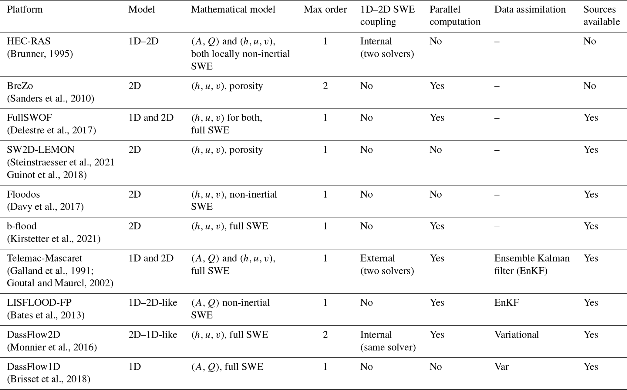
In order to combine local accuracy and computational efficiency, the association of 1D and 2D full shallow-water hydraulic models is an appropriate approach for simulating a basin-scale network in a way that is both practical and adequately accurate. Methods for coupling models of different dimensions have been developed (Miglio et al., 2005a, b; Amara et al., 2004), classically using domain decomposition (Gervasio et al., 2001) or more recently by coupling 1.5D and 2D equations, so as to model local 2D zooms of overflows overlapping with a 1D domain for in-bank flows, in a variational data assimilation framework in Gejadze and Monnier (2007) and Marin and Monnier (2009). An iterative coupling strategy is applied in Barthélémy et al. (2018) between a 1D Mascaret and a 2D Telemac operational numerical model, and a sequential data assimilation technique is performed for correcting water level forecasting. A summary of some established 1D and 2D numerical hydraulic models, external coupling methods and optimization–assimilation methods is presented in Table 1. Note that large-scale modeling of river routing–flooding is still generally performed with simplified models and/or external couplings, while enhancing the computational efficiency and realism of multi-dimensional models is important in the field of hydrological–hydraulic modeling. Furthermore, it is essential to investigate state-parameter estimation, from multi-source datasets, for improving the accuracy of hydrodynamic variables estimated with such models. Variational data assimilation (VDA) is an adequate method to tackle such high-dimensional and multi-variate hydrodynamic inverse problems from heterogeneous datasets (Lai and Monnier, 2009; Monnier et al., 2016; Brisset et al., 2018; Larnier et al., 2020; Garambois et al., 2020; Pujol et al., 2020; Malou et al., 2021). One can identify DassFlow2D (Monnier et al., 2016) as the only 2D full hydraulic model with a second-order solver with accurate wet–dry front treatment, parallel computation and adjoint-based variational data assimilation capabilities.
This work focuses on the following scientific problems: (i) the effective representation of river network flows through multi-D basin-scale hydraulic–hydrological numerical modeling, (ii) the inference from multi-source data of spatio-temporally distributed river channel parameters and inflows through a VDA approach, and (iii) the upstream informational feedback of river network observations to integrated hydrological models.
The present study details upgrades to the DassFlow variational data assimilation framework (DassFlow2D-V2, see Monnier et al., 2016) in the form of (i) a new multi-D hydraulic computational code relying on an internal mesh coupling and a single finite-volume solver and (ii) the integration and differentiation of a GR4 hydrological module, (iii) with the implementation of a regularization strategy based on Larnier et al. (2020), leading to DassFlow2D-V3.
One strength of the DassFlow platform is its variational data assimilation (VDA) algorithm. It can solve high-dimensional optimization problems with descent algorithms using gradients computed with the adjoint model. The adjoint model is obtained via the automatic differentiation tool Tapenade (Hascoet and Pascual, 2013). This allows the simultaneous inference of numerous model parameters, which may be needed over large domains. Let us remark that this is not the case for stochastic methods, where computational cost can increase dramatically with the number of sought parameters. The variational method also enables tackling multi-variate data assimilation problems, i.e., with composite control vectors (bathymetry, friction, boundary conditions, hydrological parameters), given multi-source datasets, heterogeneous in nature, and spatio-temporal resolutions (see, e.g., Brisset et al., 2018, Larnier et al., 2020, Pujol et al., 2020, and Malou et al., 2021).
To apply these unique capabilities at the scale of a river network, there is a need to develop a model with both sufficient complexity and a reasonably low computational cost. In this work, we also focus on tool simplicity, both for direct and inverse modeling, by proposing this model as a single hydraulic–hydrological tool and/or code. The proposed multi-D hydraulic code consists in a single finite-volume solver applied to a 2D river network. The network is discretized into “1D-like” reaches connected to high-resolution 2D meshes in a single formulation of the shallow-water equations (SWEs). The resulting product allows building large 1D-like river networks, connected to fine local zooms. Compared to a full 2D model, this allows computing large networks with low computational costs while maintaining the possibility to model dynamics locally at a fine scale.
The complete hydraulic–hydrological modeling of river network is achieved by coupling this hydraulic domain with a well-established conceptual hydrological model (GR4H “state–space” Santos et al., 2018) in a semi-distributed setup. The resulting integrated tool chain has been differentiated and via the VDA algorithm enables information feedback within the whole computational domain (basin) and especially from downstream to upstream.
The source code and synthetic cases presented in this study are available online (https://doi.org/10.5281/zenodo.6342723, Pujol et al., 2022), and the current updated version of the code is available upon simple request (http://www.math.univ-toulouse.fr/DassFlow, last access: 27 June 2022).
The remainder of this article is organized as follows. In Sect. 2, the modeling hypothesis, the computational resolution and inverse methods are detailed. In Sect. 3, the multi-D coupling scheme is validated on a series of academic cases and several academic and real-like inference setups are investigated. The study is concluded in Sect. 4, which also outlines potential applications and improvement perspectives that the proposed method and findings bring.
This section presents the integrated and multi-dimensional hydrological–hydraulic model and the data assimilation approach. The model is designed for simulating spatio-temporal flow variabilities over an entire river network, from upstream hydrological responses to complex flow zones (confluences, multichannel portions, floodplains, etc.).
The modeling approach which is detailed below, is based on the following ingredients:
-
an integrated multi-D hydraulic model – the 2D SWE with finite-volume solvers from Monnier et al. (2016) is applied to 1D-like–2D composite meshes of river networks using a numerical flux splitting method and an effective friction power law depending on flow depth;
-
a numerically coupled hydrological model, the widely used GR4 model from Perrin et al. (2003) in its state–space version (Santos et al., 2018), for the sake of model differentiability;
-
a computational inverse method based on VDA algorithms from Monnier et al. (2016), Brisset et al. (2018) and Larnier et al. (2020) enabling spatially distributed calibration and variational data assimilation with the whole chain.
2.1 Multi-D hydraulic–hydrological modeling principle
The flow model consists in a spatially distributed modeling of hydrological responses coupled to, i.e., inflowing, a seamless multi-scale 1D-like–2D hydraulic model of a river network within a 2D river basin domain denoted Ω⊂ℝ2 . The core idea of this work is to numerically solve the 2D shallow-water hydraulic model on a multi-D discretization 𝒟hy⊂ℝ2 of the computational hydraulic domain Ωhy⊂Ω . This discretization (mesh) 𝒟hy is composed of N mixed unstructured triangular and/or quadrangular cells with internal interfaces between 1D-like and 2D zones (see Sect. 2.2.3).
Let the basin domain Ω be composed of a hydrological domain Ωrr connected to a hydraulic domain Ωhy (Fig. 1) such that , their borders being denoted Γrr and Γhy and the hydrological–hydraulic coupling interface between Ωrr and Ωhy being denoted Γrh such that Γrh⊂Γhy. In other words, the border Γhy of the hydraulic domain Ωhy contains interfaces with the border Γrr of the hydrological domain Ωrr. Let us also consider 𝒟rr, a 2D discretization of the hydrological domain Ωrr.
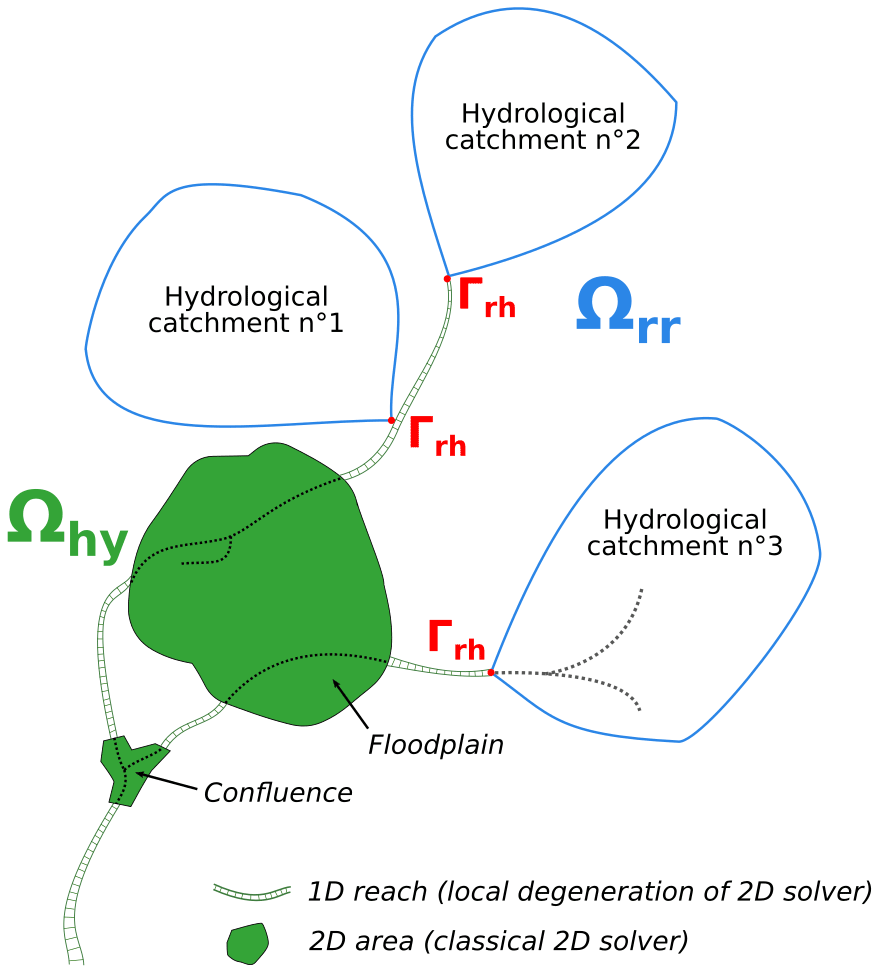
Figure 1Conceptual meshing approach for integrated hydraulic–hydrological and multi-dimensional modeling of a river network. The computational domain Ω is composed of the hydrological domain Ωrr connected to the hydraulic domain Ωhy. Ωhy contains 1D-like meshes interfaced with classical 2D meshes, Hydrological inflows generated in Ωrr can be injected into Ωhy at the Γrh domain interfaces.
Finally, an unstructured lattice covers the basin domain Ω, and a hydrological model and a hydraulic model will be resolved, respectively, on the hydrological and hydraulic subdomains and coupled via hydrological runoff flowing into the hydraulic model at the interface Γrh, as detailed in this section along with the inverse algorithm applied to the whole hydrological–hydraulic numerical chain.
2.2 Hydraulic module
Numerical hydraulic models describing open-channel flows generally rely on the resolution of cross-sectionally or depth-integrated flow equations: respectively, the 1D Saint-Venant equations or 2D SWE (see, e.g., Guinot, 2010). While 1D hydraulic models enable a physically sound representation of river flows variabilities in terms of wetted Section A and discharge Q for instance, 2D hydraulic models in flow depth h and depth-integrated velocity enable us to tackle more complex flow zones such as confluences and/or diffluences and floodplain flows. The 2D shallow-water model used in the proposed approach is presented here with the adaptation of the finite-volume solver from Monnier et al. (2016) for multi-D modeling. Note that 1D Saint-Venant equations are presented in Appendix B along with their resolution method in DassFlow1D (Brisset et al., 2018; Larnier et al., 2020), which is used for comparison in this study.
2.2.1 Mathematical flow model
On the hydraulic computational domain Ωhy⊂ℝ2 and for a time interval [0,T], the 2D SWEs with the Manning–Strickler friction term, in their conservative form, are written as follows:
with h being the water depth [m] and , the depth-averaged velocity [m s−1], being the flow state variables. g is the gravity magnitude [m s−2], b the bed elevation [m] and n the Manning–Strickler friction coefficient [s m], i.e., the flow model parameters. U is the vector of state variables and F(U) (G(U)) is its flux over the x (y) direction. Sg is a gravitational term and Sf is a friction term. Classical initial and boundary conditions adapted to real cases are considered (see Monnier et al., 2016, 2019, for details).
An effective friction law consisting in a simple power law n=αhβ is introduced, as previously done for 1D SWE for effective modeling with simplified multichannel river geometry in Garambois et al. (2017) and Brisset et al. (2018).
2.2.2 Building up equivalencies between 2D and 1D flow states
One-dimensional-like reaches refer to river reaches where the following meshing strategy has been applied: quadrangular cells are built such that their interfaces are perpendicular to the main flow direction and span the whole river (“bankfull”) width as a traditional 1D cross-section (XS) would. This leads to a series of quadrangular cells, each linked to a single upstream and downstream cell. The 1D-like approach implicitly assumes a rectangular XS shape which potentially impacts the representation of (i) a section hydraulic geometry (Leopold and Maddock, 1953) and (ii) longitudinal hydraulic controls and flow variabilities.
With a view to putting the multi-D model in coherence with real flow physics, a continuity condition between 1D and 1D-like models states and parameters is required. This continuity condition is enforced at a section, in a prismatic channel such that the uniform permanent flows, that is, equilibrium, are preserved.
Let us consider a reference 1D model in (A,Q) variables with the bankfull width value W1D. The friction term reads (Appendix B). In the corresponding 1D-like model in variables (see Sect. 2.2.1), the friction term reads
Considering 1D flow states over an idealized river section (Fig. 2a) and the hypothesis of local flow equilibrium (uniform, steady-state) with identical wetted areas A and water surface (WS) widths W, the continuity condition implies that
where n1Dlike (h1Dlike) is the Manning–Strickler friction coefficient (flow depth) in the 1D-like model i.e., the coefficient in the 2D SWE (Eq. 1).
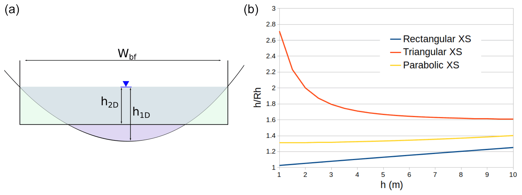
Figure 2Equivalency of 1D and 2D flow states at equilibrium (permanent uniform flows): effective friction and bathymetry. (a) Equivalency between a 1D idealized XS (blue) and a 2D single-cell rectangular XS (green), with the same flow section A and WS elevation. (b) Variation in the hydraulic radius Rh(h) for three XS shapes (of similar dimensions). This showcases the potential over- and underestimation of state variables using “1D-like equivalent friction” from Eq. (2).
With the additional assumption of a rectangular XS (as it will be assumed in some test cases), we have , which leads to .
This “1D-like equivalent friction” leads to a perfect fit in WS elevation of a 1D-like model and a 1D model in a straight prismatic channel at the given uniform regime (results not shown here for brevity). Figure 2b shows the evolution of the ratio vs. h. For rectangular and parabolic XS, the ratio is expected to increase with h. Thus, one can naturally expect an overestimation (underestimation) of the actual friction coefficient by n1Dlike at lower flows (greater flows). This would lead to an overestimation (underestimation) of the 1D WS elevation by the “equivalent” 1D-like model. However, later it will be considered a power law in h to model the friction coefficient (Sect. 2.2.1), which provides a better fit to the 1D WS elevations outside of the considered permanent flow.
Note that longitudinal controls and flow variabilities in 1D-like models are assessed using synthetic cases in Sect. 3.2.4.
2.2.3 Multi-dimensional hydraulic model
Over a given cell K∈Ωhy of area mK, the piecewise constant values are approximated. Recall that the finite-volume approach applied to the homogeneous part of the hyperbolic system of Eq. (1) (that is, without the friction source term Sf but including a consistent discretization of the gravitational source term Sg) is written as follows:
where and are the piecewise constant approximations of at time tn and tn+1 (with ), and Fe stands for Riemann fluxes through each edge e of the border ∂K of the cell K, with each adjacent cell Ke. The length of edge e is me, and ne,K is the unit normal to e oriented from K to Ke.
The finite-volume schemes are those developed in Couderc et al. (2013) and Monnier et al. (2016). The discretization of the friction source term is described in Appendix A.
Based on the first- and second-order finite-volume solvers of Couderc et al. (2013) and Monnier et al. (2016), a “1D–2D” coupling technique is introduced following a similar concept to Finaud-Guyot et al. (2018) (urban geometries and porosity context) to compute numerical fluxes on each interface between a 1D-like quadrangular mesh cell connected to several 2D cells as schematized in Fig. 3.
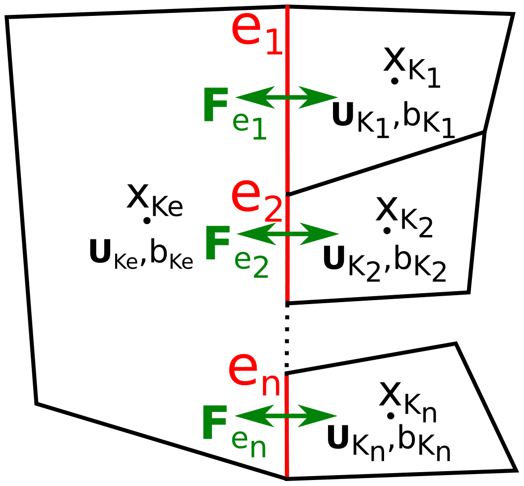
Figure 3Internal multi-D domain interface, general case. At each cell center x, the state variables and the bathymetry b are defined. The total numerical flux is conserved: .
At the multi-D interfaces, that is, in the case of n>1 cells xK,i i∈[1…n] adjacent to the same interface of another cell Ke (see Fig. 3 for notations and Sect. 3.3.2 for a real-like example), a special treatment is applied. It consists in the Riemann fluxes being calculated for each cell Ki using the state from the same corresponding Ke cell over an interface of length . In the end, the flux crossing the interface is equal to the sum of the fluxes crossing the ei interfaces: .
This type of internal interface has been implemented in the numerical solvers from Monnier et al. (2016) in the DassFlow platform, which includes a solver with second-order accuracy in space. This solver, developed in Couderc et al. (2013) and Monnier et al. (2016), is accurate and robust for wet–dry front propagations and fully applies in the present context. Note that the lateral distribution of variables across the 1D–2D interface is not constrained. The source code and synthetic cases are available upon simple request.
2.3 Hydrological module
In order to simulate the hydrological response of upstream and lateral sub-catchments flowing into the river network within a river basin, a hydrological module is coupled to the 2D SW hydraulic model, in a semi-distributed manner for simplicity here.
Over the hydrological domain Ωrr, we consider the discretization 𝒟rr here into C sub-catchments and corresponding disjointed sub-domains , the outlet coordinates of which are . For a given sub-catchment, the hydrological model is a dynamic operator, consisting in coupled state equations (ordinary differential equations, ODEs) and output equations, that reads
where h(x,t) is the state variable vector, P(x,t) and E(x,t) is the observable rainfall and evapotranspiration inputs (here spatially averaged over the area of each sub-catchment i for semi-distributed modeling), Q(x,t) is the “observable” output discharge, and θ(x) is the “unobservable” parameter vector.
The widely used, parsimonious and robust conceptual hydrological model GR4 (Perrin et al., 2003), in its state–space version from Santos et al. (2018), was chosen in this study for parsimony and differentiability reasons. The original lumped hydrological numerical model has been deployed in a semi-distributed manner in the DassFlow framework.
The model is composed of two non-linear stores for production (soil moisture accounting) and routing and a Nash cascade composed of a series of linear stores replacing the unit hydrograph from Perrin et al. (2003). Being a set of ODEs with explicit dependency to parameters, this hydrological model (Eq. 4, see detailed GR4 equations in Appendix C) is differentiable. Moreover, the Fortran code is differentiable with the automatic differentiation tool Tapenade (Hascoet and Pascual, 2013).
The evolution of reservoir states and model outputs and inputs is presented for a sample rain event in Fig. 4.
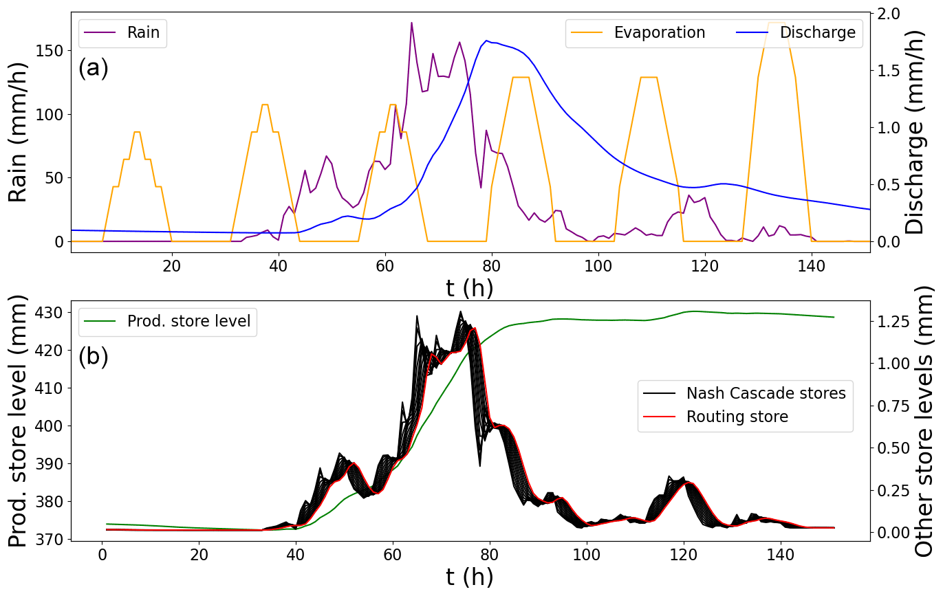
Figure 4Evolution of GR4 inputs, output and reservoirs states during a sample rain event. (a) Temporal forcings (rain and evaporation) and modeled output (discharge). (b) Hydrological model states (reservoir levels).
The input of the hydrological model is the evapotranspiration and precipitation En and Pn; the output is discharge [mm h−1]. En and Pn are classically imposed from data time series as a piecewise constant at the fixed temporal resolution (e.g., hourly). The numerical resolution is achieved with an implicit Euler algorithm with an adaptive sub-step algorithm enabling us to reduce numerical errors especially for high flows (Santos et al., 2018). The initial states of the stores is given by a 1-year warm-up run. The discharge q is injected into Ωhy at a sub-interface of Γhy-rr, either as an upstream or lateral flow.
The calibrated parameters will be the classical four parameters of GR4, i.e., the reservoir capacities in millimeters for each sub-catchment i∈1…C. They will constitute the parameter vector θrr considered in the forthcoming VDA experiments. Other parameters, such as several drainage law exponents or the number of Nash cascade stores, are not optimized as classically done with the GR4 model (Perrin et al., 2003). They are set at values from Santos et al. (2018).
2.4 Inverse algorithm: variational data assimilation
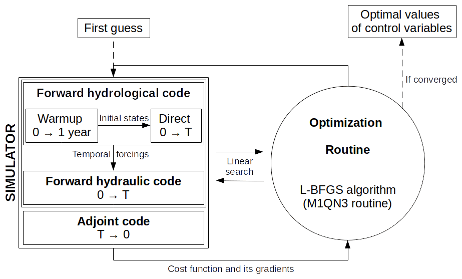
Given spatio-temporal flow observables, provided by in situ and airborne sensors for instance, the inverse algorithm consisting in variational data assimilation (VDA) aims at estimating the unknown or uncertain “input parameters” of the hydrological–hydraulic chain composed of a hydraulic model, presented in Sect. 2.2, and a hydrological model, presented in Sect. 2.3. Detailed know-how on VDA may be found in online courses (see, e.g., Bouttier and Courtier, 2002, and Monnier, 2014). This group of VDA algorithms relies on cost gradients, i.e., variations, here computed by the adjoint model, to minimize a misfit to the observed reality (see Fig. 5). The adjoint model of the whole toolchain composed of DassFlow multi-D with GR4 modules is obtained by automatic differentiation with the Tapenade engine (Hascoet and Pascual, 2013). Note that 2D, 1D-like and 1D–2D models are functionally identical from the point of view of the adjoint code and the assimilation process.
We consider the following set of spatio-temporal observations of water surface and discharge over the river domain Ω⊂ℝ2:
with Zo the observed WS elevation [m] above reference elevation, Qo the observed discharge [m3 s−1], No,Z the number of altimetric observation points and No,Q the number of observed discharges over Ω.
Note that observed discharge Qo may be a value of a hydraulic discharge at a flow XS in Ωhy or within the hydrological domain Ωrr and especially at the outlet of a sub-catchment here. Also note that other water surface observables could be considered, such as water surface velocity observations or dynamic water masks, but this is beyond the scope of this study.
Given river stage and/or discharge observations, the aim here is to estimate unknown or uncertain quantities of the hydrological–hydraulic model among discharge hydrographs on the border of the hydraulic domain (in 1D-like and/or 2D parts), spatially distributed hydraulic parameters over a river network (bathymetry elevation b or friction n) and hydrological parameters for all sub-catchments .
The control vector containing the sought quantities is denoted θ in what follows:
with θhy and θrr the control vectors of, respectively, the hydraulic and the hydrological modules, N the number of inflows control points in space and T the number of inflow values in time, M the number of bathymetry-friction control cells, and P the number of hydrological units.
We consider a cost function jobs aiming at measuring the discrepancy between simulated and observed flow quantities on the hydraulic–hydrological computational domain Ω. This cost function is defined as
This cost function contains either misfit to WS elevation, , or misfit to discharge, .
The metrics (symmetric positive definite matrices) 𝒪𝒵 and 𝒪𝒬 are based on the inverse of the observation error covariances. This enables us to regularize the inverse problem; see, e.g., Bouttier and Courtier, 2002, Monnier, 2021, Asch et al., 2016, and references therein for related discussions.
Moreover, we classically enrich the cost function with a regularization term: with jreg a Tikhonov-type regularization term. Here we consider a regularization on the bathymetry only: with θ defined by Eq. (6).
The regularization term adds convexity to the cost function. Moreover, it here dampens the bathymetry highest frequencies. Recall that low Froude flows; i.e., subcritical flows naturally act as a low-pass filtering of the bathymetry shape; see Martin and Monnier (2015) and Gudmundsson (2003).
The total cost function j is minimized starting from a background value θ(0). Following Lorenc et al. (2000) (see also Larnier et al., 2020), the following change in variables is applied:
with B being the covariance matrix of the background error.
Then by setting J(k)=j(θ), the optimization problem which is solved is actually the following:
The first-order optimality condition of this optimization problem (Eq. 9) reads . The change in variables based on the covariance matrix B acts as a preconditioning of the optimization problem. This optimization problem is solved using a first-order gradient-based algorithm, more precisely the classical limited-memory Broyden–Fletcher–Goldfarb–Shanno (L-BFGS) quasi-Newton algorithm (Zhu et al., 1997) or, in some cases in this study, its bounded version L-BFGS-B (Zhu et al., 1997) but without variable change (Eq. 8).
The choice of the covariance matrix B, represents an important a priori information and greatly influences the computed solution of the inverse problem. Assuming the unknown parameters are independent variables, the matrix B is defined as a block diagonal matrix:
Each block matrix of is defined as a covariance matrix (positive definite matrix) using 2D kernels for spatial controls. Here following Larnier et al. (2020), we consider
The parameters LQ and (Lb,Ln) act as correlation lengths. These parameters are usually empirically defined. However the expression of Bb and the correlation lengths can be derived from physically based estimations following Malou and Monnier (2021).
The following stopping criteria are used to stop the iterative optimization process if (i) the cost function does not decrease over a set number of iterations or (ii) the current cost gradient, normalized by the initial cost gradient, goes under a set objective value. The multi-D hydrological–hydraulic tool chain presented above has been implemented in the latest version of Monnier et al. (2019).
3.1 Numerical experiments design
Both synthetic and real cases are considered to test the forward and inverse modeling capabilities of the proposed computational chain for river network and floodplain simulation.
First, the multi-D hydraulic model (Sect. 2.2.3) is validated against reference hydraulic models on synthetic cases corresponding to typical hydraulic complexities: (i) simple straight channel, (ii) confluence, and (iii) straight, rectangular and parabolic, channels with effective parameterization of friction and bathymetry. For fluvial regimes in the context of altimetry, these hydraulic complexities generate hydraulic controls. Following Montazem et al. (2019), we define hydraulic controls as characterized by a maximal deviation of the water depth from the normal depth (see, e.g., Chow, 1959, and Dingman, 2009, for definition) at the reach scale.
A series of inference cases are considered in twin experiment setups. In a twin experiment, a reference model acts as a synthetic truth and is used to generate observations of model variables (e.g., b+h in Ωhy or Q in Ωrr). No observation noise is considered in this study. The VDA method is then applied with these observations on an altered version of the reference model. Inferences of temporal forcings, channel parameters and hydrological parameters are carried out.
3.2 Synthetic cases
First, the proposed multi-D hydraulic solver (Sect. 2.2.3) is evaluated and compared to a fine 2D reference model on two simple configurations, a straight channel and a confluence, that feature frontal interfaces between 1D-like and 2D meshes. Next, to investigate the reproducibility of hydraulic controls using a 1D-like meshing approach and effective modeling, this approach is compared to a 1D reference model in three typical channel configurations. Finally, inferences of inflow hydrographs and of a friction power law n=αhβ are carried out using WS observables.
3.2.1 Forward multi-D hydraulic cases
Straight channel case
A prismatic rectangular channel and a multi-D mesh are considered (1D-like to 2D to 1D-like, see Fig. 6). The channel width is 300 m and its length is 2300 m. A rating curve is imposed downstream. This multi-D model is compared to a reference 2D model with a refined mesh (mesh not shown, 2400 cells, average edge length ∽25 m). The multi-D waterline is validated against the 2D model at permanent flow and the modeled downstream discharges are compared for a flood hydrograph (Fig. 6b). Both first- (not shown) and second-order numerical solvers allow a close fit to the target water line (Fig. 6a, bottom diagram).
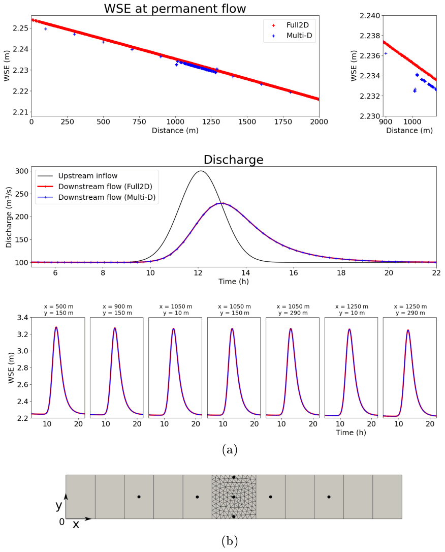
Figure 6Multi-D straight channel case results with second-order scheme. The flow is subcritical with a maximum Froude value of 0.06. (a) Top: waterlines for a permanent flow of 100 m3 s−1: reference 2D waterline (red); waterline for the mesh in (b) (blue);he total misfit at the 1D–2D upstream interface (at 1000 m) is around 10−3 m, for a relative misfit <0.15 % of the local depth. Middle: upstream discharge during sample varied flow event (blue); downstream simulated flow for the considered meshes (total overlap; red/blue). Bottom: WS elevation observations for the varied flow event (total overlap). (b) Multi-D mesh. Station locations are noted as blue dots.
At permanent flow, a slight misfit is observed between the 2D and multi-D WS elevations with the second-order scheme (Fig. 6a, top diagram, relative misfit <0.15 % at 1000 m). This is due to the approximation error in the multi-D model caused by large spatial steps in 1D-like reaches (dx=200 m). Indeed, this misfit is reduced by reducing the 1D-like cell length (not shown). This is confirmed and showcased in the next subsection.
At the interface between 1D-like and 2D meshes, a slight jump in WS elevations can be observed at all 2D cells (Fig. 6a, top diagram). This is due to the second-order scheme, which is currently not designed for multi-D interfaces. Recall that no constraint is imposed on the lateral distribution of computed variables. The technical implementation of this reconstruction for 1D–2D interfaces will be done in the next version of DassFlow.
During a varied flow event, the outflow of both models is close to identical (Fig. 6a, middle diagram). The flow is correctly transmitted at multi-D interfaces and, at this scale, the 1D-like meshes are adequate to model a flood wave propagation.
Simple confluence case
A simple symmetrical confluence is modeled using a multi-D mesh. The channel width is 300 m in the downstream reach and 150 m in the upstream reaches. Two inflow hydrographs are imposed at the two upstream interfaces. The maximum abscissa of the mesh points are 0 and 2075 m. The 2D part (average edge length ∽5 m) contains a confluence flow zone (Fig. 6), while the 1D-like mesh (dx=100 m) covers the upstream and downstream reaches. At permanent flow, the multi-D model compares well with the reference 2D fine model (mesh not shown, 15 000 cells, average edge length ∽5 m) and leads to similar conclusions to the above paragraphs. Using a shorter spatial step in the 1D-like reaches (10 m) reduces the difference between reference and multi-D model and allows for a nearly perfect fit to the reference WS elevation at permanent flow (Fig. 6a, middle diagram). During a varied flow event, the outflows modeled with the multi-D model are very close to reference ones: slight differences during rising and falling limbs, same peak time, and Nash–Sutcliffe efficiency (NSE) =0.996.
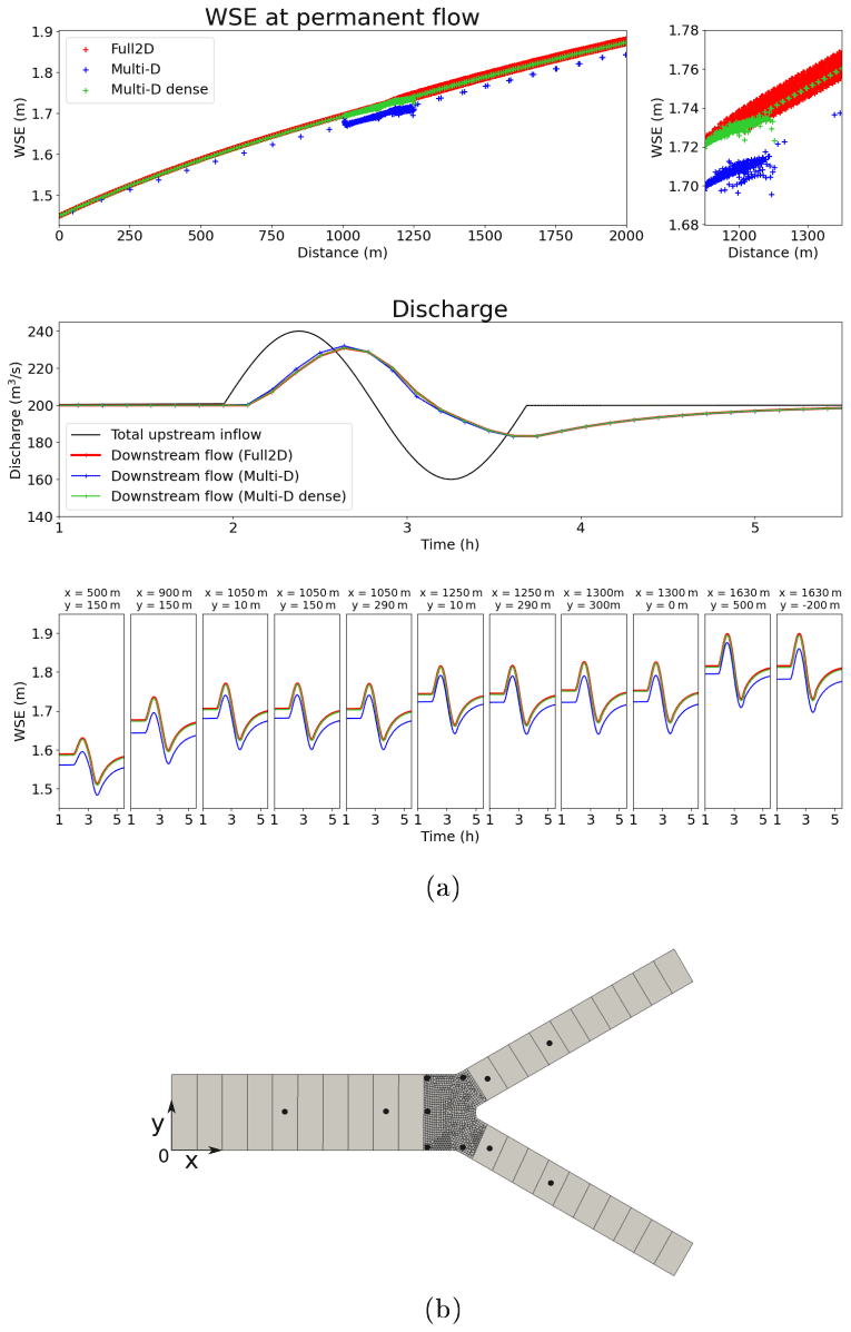
Figure 7Multi-D confluence case results with second-order scheme. (a) Top: waterlines for a permanent flow of 100 m3 s−1 at both upstream boundaries; reference 2D waterline (red); waterline for the mesh in (b) (blue); waterline for a denser 1D–2D mesh (not shown, green). Middle: total upstream discharge during sample varied flow event (evenly distributed between upstream boundaries, blue); downstream simulated flow for the considered meshes (red/green/blue). Bottom: WS elevation observations for the varied flow event. (b) Multi-D mesh. Station locations are noted as black dots.
Hydraulic controls and effective friction
To investigate the reproducibility of hydraulic controls for fluvial flows, which are characterized by a maximal deviation of the water depth from the normal depth at the reach scale (see definition in Montazem et al., 2019), using a 1D-like approach, a set of typical channel variabilities and hydraulic controls are considered. Let us compare 1D and 1D-like waterlines in a series of synthetic cases: (i) a straight rectangular channel, (ii) a straight rectangular channel with a mid-channel slope break and (iii) a straight parabolic channel.
Direct calibration
Recall the equivalent friction formulation (Eq. 2) designed to match the water line at a section and at equilibrium. For each 1D-like case, waterlines with 1D friction () and effective equivalent friction are generated. Effective friction values are calculated using Eq. (2) and results from the corresponding 1D case. Reference 1D flow lines are computed with DassFlow solving 1D Saint-Venant equations in (A,Q) state variables with a Preissmann scheme (see Appendix B and also Larnier et al., 2020).
In a straight rectangular prismatic channel, with the 1D normal water depth imposed downstream (Fig. 8a), a backwater curve is computed by the DassFlow1D model (in red). With a 1D homogeneous friction (), the 1D-like approach yields an underestimated waterline (in blue). A homogeneous effective friction allows us to correct the underestimation and to better match the 1D normal water depth over the whole domain (in green). The remaining misfit can be attributed to numerical errors, especially numerical diffusion from the Preissmann scheme (1D model spatial step is dx1D=100 m).
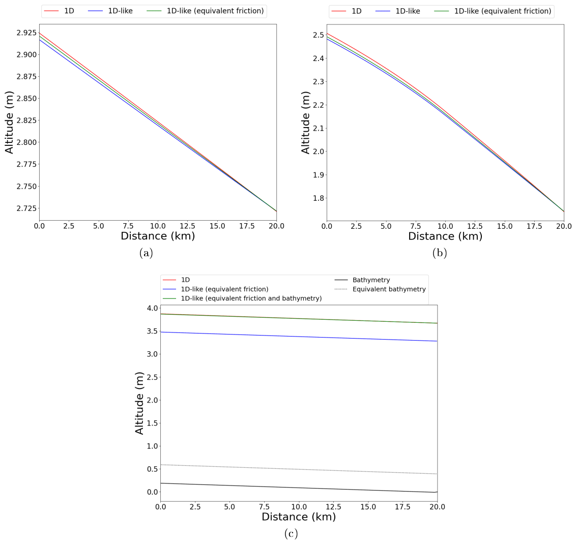
Figure 8Effective friction analysis for steady waterline in academic cases: (a) rectangular channel with constant slope, (b) rectangular channel with slope break, (c) parabolic channel with constant slope. Values of effective friction parameter α : (a) , (b) , , (c) . Bathymetric shift δb [m]: (a) 0, (b) 0, (c) 0.591. One-dimensional reference model: fixed time step 5 s, spatial step 100 m. Average Courant number equals 0.26 1D-like models: adaptive time step with mean value of 9 s. One-dimensional-like cell length 100 m; average Courant number equals 0.48.
A first complexification of this case consists in the introduction of a local hydraulic control point in the form of a slope break at x=10 km (Fig. 8b). In this setup, both 1D and 1D-like models generate M2 backwater curves; see, e.g., Dingman (2009). The hydraulic control generated at the slope break is well represented with a 1D-like approach, given the aforementioned numerical errors due to the coarse grid.
Another complexification of the first case consists in changing from a rectangular XS to a parabolic one (Fig. 2). In this case, both equivalent friction – a single homogeneous patch – and effective bathymetry, in the form of a homogeneous shift δb of the reference bathymetry, are needed to match the 1D WS elevation. Equivalent friction only allows us to model identical wetted sections at permanent bankfull flow for a given channel width (Sect. 2.2.2). In this case, matching the 1D wetted section does not equate to matching its WS elevation; thus an effective bathymetry is used.
According to the above model comparisons, effective parameterization of channel parameters is sufficient to reproduce 1D behaviors with a 1D-like approach for permanent bankfull flows in simple geometries. Outside of the permanent bankfull flow, a friction power law n=αhβ can be used (Sect. 2.2.1). This friction aims at better 1D-like representativity when modeled wetted surfaces (and other XS variables) are different in 1D and 1D-like models for the same WS elevation.
Inverse calibration
In the following comparison, power-law parameters α and β are obtained using VDA in a twin experiment setup. Observations are taken at two stations (Fig. 9). Prior values are α=0.05 s m and β=0.
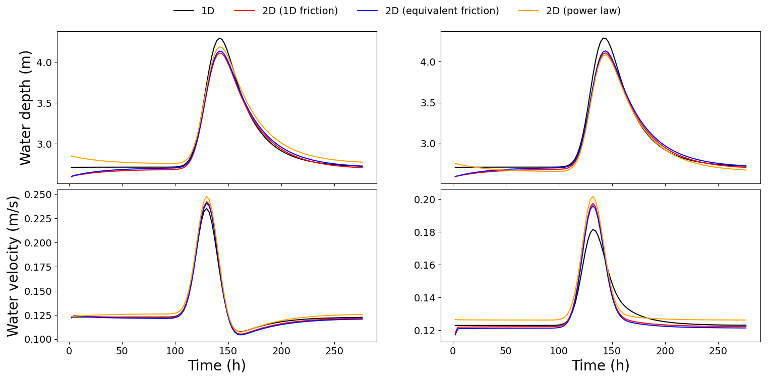
Figure 9Effective friction analysis for an unsteady waterline in case (i). The power law is given by n=αhβ, with α=0.0446 and β=0.0634. The injected hydrograph is symmetrical. observation stations are at x=2.5 km and x=7.5 km. Adaptive time step with average value of 13 s. One-dimensional-like cell length: 200 m. Average Courant number: 0.33.
The classic friction law and a power law with calibrated parameters are compared in Fig. 9 during a varied flow event (assimilation time window of 270 d). A range of water depth higher than the bankfull depth used to calculate equivalent friction parameters is simulated. This results in an increase in misfit to the 1D WS elevation at high flow (Fig. 9, in blue and red). The calibrated friction power law (in orange) somewhat reduces the misfit during high flows in this simple synthetic channel and within the simulated water depth range.
3.2.2 Multi-D hydraulic–hydrological data assimilation
Temporal forcing inference
Simple inference tests are carried on the confluence case from Sect. 3.2.1, following Pujol et al. (2020), in a twin experiment setup. A control vector is considered, where Q1 and Q2 are sinusoidal inflow hydrographs injected at the upstream cell of the two upstream reaches. Pujol et al. (2020) shows that the minimal requirement to infer multiple spatially distributed temporal forcings simultaneously is to observe either (i) both of their “unmixed” signatures, at one point each, or (ii) one of their unmixed signatures at one point and their mixed signatures at a second point. We verify this for configuration (ii). Unmixed signature observations are generated at a 1D-like cell of the upstream reaches; mixed signature observations are generated at a cell in the 2D part (Fig. 10a, red crosses). Prior values for the inflow hydrographs are constant and set to their average value . Using sets of two observation points over a 5 h period (see Fig. 10), we are able to reproduce the results of Pujol et al. (2020) but with the proposed multi-D hydraulic model: the VDA algorithm enables us to infer Q1 and Q2 close to perfectly from configurations (i) and (ii) (Fig. 10b).
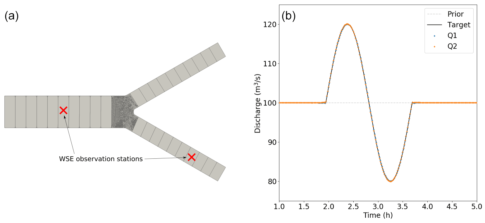
Figure 10Inflow hydrographs inference on confluence synthetic case in observation setup (b) with one station on a reach upstream of the confluence and one observing mixed flows downstream in the 2D part. Given sufficient observability and an unbiased prior, inferred hydrographs (in blue and orange) are both at target (blue, total overlap). The flow is subcritical with a maximum Froude value of 0.05.
Hydrological parameter inference
In this second twin experiment, the issue of the spatially distributed calibration of a hydrological model is studied, from multi-source observations of the river network. The confluence case above is used and this time, the upstream inflows are generated by the GR4H module applied to two upstream catchments flowing into the hydraulic module. For each catchment, synthetic rain and evaporation time series and a hydrological parameter set are used to generate a discharge time series over a 1-year period (not shown). Mixed observables are used: WS elevation is observed at a single downstream point, and hydrological model discharge is observed at the outlet of one of the catchments, over 360 d. They provide the same signal observability – mixed and unmixed signals – as in the above paragraph but with observations of a different nature. Since the observed variables are of a different nature and amplitude, we introduce a normalization. The cost function is here , with each term being normalized by the number of observations and by their range of variation such that
and
Those correspond to two separate normalized squared RMSE with No,Q and No,Z denoting the number of observation stations and TQ and TZ the number of observation time steps.
The control vector contains the two sets of four hydrological parameters each. For this synthetic case, an inequality constraint of the control parameters is imposed with the bounded L-BFGS-B algorithm (Zhu et al., 1997). Indeed, restricted research intervals are considered for the three first parameters of each catchment, namely a 5 % bracket around their target values used as a prior, while c4 is sought in its expected variation range from an erroneous prior (Table 2). Expected ranges for GR4H parameters are provided in Le Lay (2006), for the classical GR4 formulation.
Table 2Hydrological parameter inference results. Prior values are taken as identical to target values, except for parameter c4, where under- and overestimated prior value are considered. Inferred values for all parameters including c4 are very close to the target. The “/” separates values for the two distinct hydrological units.
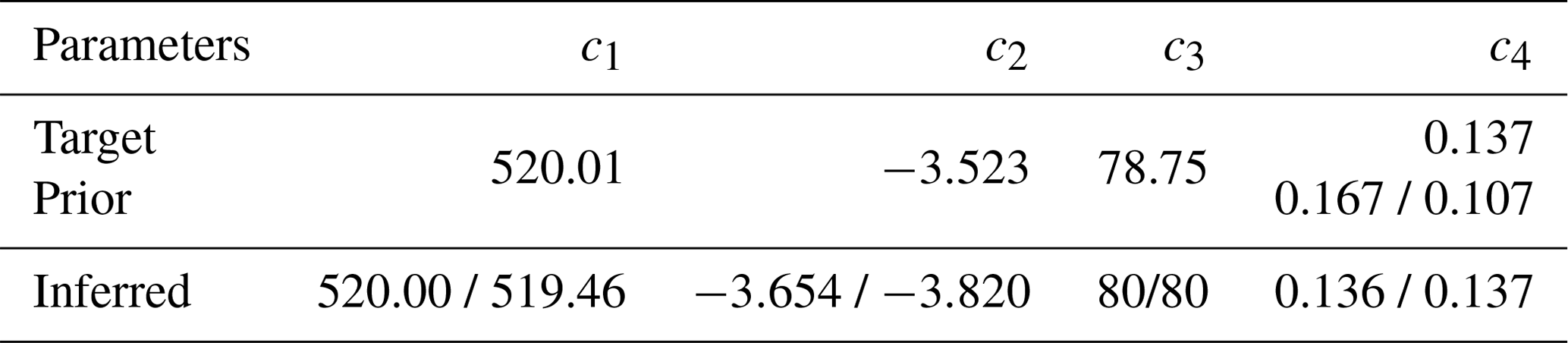
In this setup, both jQ and jZ are reduced during the iterative steps and the inferred value for both c4 parameters are very close to the target value starting from an erroneous prior (Fig. 11b). Bounded parameters c1 and c2 vary slightly between their bounds, while c3 is locked at its lower bound from the first iteration.
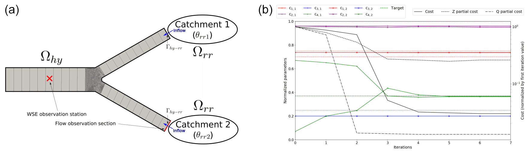
Figure 11Simultaneous inference of GR4H hydrological parameters in two catchments from multi-source observations: WS elevation and flow observations. (a) Multi-D hydraulic mesh and modeled hydrological catchments. Hydrological discharge at the outlet of Ωrr flows in upstream in Ωhy. Observation stations (red cross and red line) are used for inferring hydrological parameters. (b) Inference of two sets of four hydrological parameters: normalized costs and parameter values over the course of the iterative optimum search. The x4 background values are erroneous. x1, x2 and x4 background values are set to target values.
3.3 Real cases
3.3.1 Garonne River: 1D-like effective model of a 2D reference case
A 1D-like model of a reach of the Garonne River, in southern France, is built from real data and calibrated here via assimilation of spatially distributed WS observations in a twin experiment setup. A full 2D model of 75 km of the Garonne River (not shown, 867 500 cells including floodplains, average edge length ∽25 m) is used to generate real-like observables on this well-known case (Garambois and Monnier, 2015; Brisset et al., 2018; Larnier et al., 2020; Monnier et al., 2016). First, river extent is derived from the 2D model output at bankfull flow Q=400 m3 s−1 with a homogeneous friction n=0.05 s m. This extent is in turn used to build a 1D-like mesh, over the whole reach: single quadrangular cells cover the whole river width and are linked sequentially along the river reach (Fig. 12). One-dimensional-like cell interfaces are perpendicular to the flow direction, as would be cross sections (XSs) in a 1D model. Each cell is about 100 m in longitudinal length. This mesh was generated using the SMS.1 Cell bathymetry is first set using the lowest bathymetry point at each corresponding 2D XS.
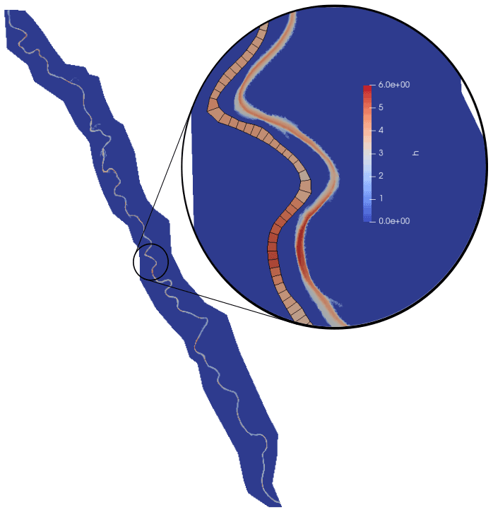
Figure 12Garonne 2D model extent and simulated water depths using the 2D model and the 1D-like model for a non-flooding event. In the zoom, both models are represented, with a slight longitudinal shift for the 1D-like model, to allow qualitative comparison of both simulated water depth and water surface extents.
Permanent bankfull flow calibration
A first expectedly imperfect 1D-like model (Model A1) is built using the 1D-like coarse mesh and expectedly underestimated bathymetry elevation and a homogeneous friction parameter of 0.05 s m. The simulated steady WS elevation at bankfull flow is lower than that of the 2D model (average misfit of 0.858 m), which is expected since the 1D bathymetry is that of the lowest point of the 2D XS (Fig. 2). Furthermore, the 1D-like friction is underestimated and leads to an underestimated simulated water depth (and flow surface). The WS elevation misfit does not seem to follow a significant trend from upstream to downstream, although it varies sharply at points of width variation (Fig. 13, e.g., around cell 410). Recall that the goal of this effective modeling approach is to accurately reproduce water surface signatures, including WS elevation and, tangentially, flow section (Sect. 2.2.2).
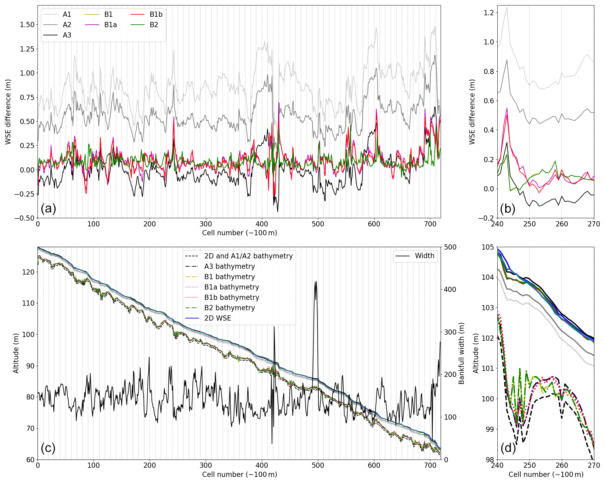
Figure 13Comparison of seven 1D-like models of 72 km of the Garonne River to a reference 2D SW fine model for a permanent flow (reference WS elevation in blue lines, c, d). (a) WS comparison of 1D-like models to 2D reference model at each spatial point. (b) Zoom on 3 km long reach of interest. (c) WS elevation and bathymetry for the reference and 1D like models. (d) Zoom on 3 km long reach of interest. For models A1, A2 and A3 (in gray), the bathymetry and homogeneous friction are manually calibrated. For mode B1 (yellow), B1a (magenta), B1b (red) and B2 (green), the bathymetry and friction are calibrated by VDA. For models B1 and B2, inferences are carried out from observations at each cell (720 total). For models B1a and B1b, inferences are carried out from observations every 10 cells (i.e., around every 1 km, 72 stations total). Vertical bars indicate these 72 stations.
Calibration by hand. We here propose to reduce the misfit using, on the one hand, effective friction and, on the other hand, bathymetry as follows. In Model A2, the introduction of an equivalent friction parameter (Eq. 2), calculated at each 1D cell using observations from 2D XS, improves the WS elevation misfit (mean friction of n=0.062 s m, average WS elevation misfit of 0.562 m). It reduces misfit overall but has no significant local influence (Fig. 13). In Model A3, we use the average WS elevation misfit from Model A2 to create a simple bathymetry shift δb that helps fit the observations. Equivalent friction parameters from Model A2 are kept and all bathymetry points are shifted by δb=0.562 m (the bottom slope is conserved). The average WS elevation misfit at bankfull flow reaches 0.003 m for Model A3, which is a very satisfying result.
Calibration by VDA. Now, the same calibration problem is addressed with an inference based on the VDA method. It is applied to the same reference model permanent flow waterline, observed at each cell. The control vector contains a single homogeneous friction parameter, as before, and spatialized bathymetry b(x) for each cell. To constrain the parameter search, two VDA processes are performed separately: a bathymetry regularization and a change in variable. Inference with bathymetry regularization leads to Model B1, with γ=1 (Sect. 2.4). Inference with change in variable (Eq. 8) leads to Model B2, with Lb=500 m (Eq. 11). Both models lead to average misfits close to that of Model A3: 0.0839 and 0.0844 m, respectively.
Two other inference setups based on Model B1 are considered. The number of observations is divided by 10: 72 stations, homogeneously distributed at 1 per each 1 km, are considered. In Model B1a, no regularization term is considered (γ=0). In Model B1b, a regularization is added (γ=1, chosen by trial and error). This weight can be optimally determined using iterative regularization (Malou and Monnier, 2022). It is dependent on the spatial scales of observed signals and on the discretization of inferred parameters. As presented in Fig. 13 and in Table 3, both inferences lead to low misfits of the 2D permanent WS elevation. The regularization tends to reduce extreme bathymetric variations that tend to appear far from the observation points. The iterative minimization process can be followed through the cost function value and the parameter gradients (Fig. 14). Values are normalized over their initial (iteration 0) value. For Model B1a, the optimal control is reached after 40 iteration (for a normalized cost of ), while for Model B1b it is reached in 85 iterations (for a normalized cost of ). Both models follow the same trajectory up to around iteration 12, where the regularization term jreg reaches the same order of scale as the WS elevation misfit term jobs.
Variational calibration of the channel parameter has allowed us to fit a permanent regime water line. The following paragraphs study the reproduction of propagation in a calibrated model during a varied flow event.
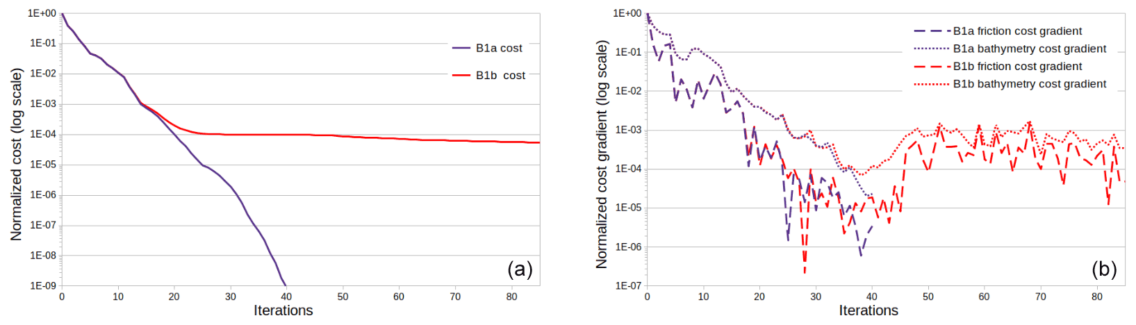
Figure 14Normalized cost functions and gradients for inferences of distributed bathymetry and homogeneous friction, from 72 observation stations, in models B1a and B1b. (a) Total cost normalized by initial cost vs. iterations. (b) Cost gradients normalized by initial gradient for the inferred parameters vs. iterations.
Table 3Garonne models parameters and metrics. “PR” stand for permanent regime (discharge of 400 m3 s−1). The “varied” flow event is non-flooding and has a mean discharge of 398 m3 s−1, with a minimum of 183 m3 s−1 and a maximum of 702 m3 s−1. “High” observation density corresponds to 720 stations or one station per 100 m. “Low” observation density corresponds to 72 stations or one station per 1 km.

Variational calibration for a flow event
Let us now consider a varied flow event, without flooding in the 2D model. This event lasts 10 d, with a peak discharge of 702 m3 s−1 at the start of day 2, a minimum discharge of 160 m3 s−1 and an average discharge of 382 m3 s−1. Given our previous inference attempts, we know that we can find a couple (n,b(x)) or (n,δb) that minimizes the average misfit. For the sake of simplicity, we consider the couple (n,δb). For a varied flow event, this couple would be an optimal parameterization for the average observed water line. A first inference trial is carried out for a densely observed (in space and time) varied flow. This dense observability is not meant to imitate the actual observability of real rivers but to provide sufficient constraints for the considered inverse problem, with the aim to showcase the capability of the variational toolchain and 1D-like model to fit fine-scale real-like water surface elevation (WSE) variations (see hydraulic parameter inference from sparse uneven altimetric observations of river surface in Brisset et al., 2018, Larnier et al., 2020, Garambois et al., 2020, and Pujol et al., 2020).
Using Model A1 as a prior for bathymetry and friction and observations from the 2D model, we find the following optimal parameters: . The resulting optimal model is Model C. To allow a better fit during high and low flows, we introduce the friction power law n=αhβ (Sect. 2.2.1). Using observations from the 2D model during the varied flow event, we infer the couple (β,δb). The value of α is set to 0.054 s m, the inferred value from Model D. Three different β priors are tested: −0.5, 0, 0.5. δb is included in the control vector to allow modeling of more varied water depths, which may be needed to reach the optimum. All three inferences lead to the very close optimal control. Their averaging, a slight bathymetric shift δb=0.099 m and , leads to Model D. The direct simulation results of Model D are compared to the reference model. They correspond to an average WS elevation misfit of 0.026 m at high flow and of 0.11 m at low flow. Compared to Model C (average misfit of 0.086 and 0.20 m at, respectively, high and low flow), this is an improvement. Note that NSE values for both model (Table 3) are both extremely close to 1.
The variational calibration of the global bathymetric shift δb and of a homogeneous friction value n in a 1D-like model has allowed us to closely fit WS elevation observations of a 10 d flood wave over the reference Garonne model. The calibration of depth-dependent friction, in the form of the β parameter in n=αhβ, has allowed an even closer fit to this reference WS elevation over the high and low flows, i.e., a better representation of the observed flood wave propagation.
3.3.2 Adour basin: multi-D hydrological–hydraulic model
The whole hydrological-multi-D hydraulic tool chain is now tested in a real context both for forward and inverse problem resolution. A real and complex basin case is now considered: the Adour River basin in the southwest of France, with a total drained area of 16 890 km2 at the estuary. It is probably one of the most difficult basins to model in the country because of contrasted hydrological regimes including nival effects in the south, flash floods on small ungauged catchments, complex river network morphology, anthropized floodplains and tidal effects from downstream areas.
In this section, a multi-D model, composed of 1D-like meshes and 2D zooms over the floodplain area is built from available data (Fig. 15, 2D area in green). Then, forward and inverse flow simulations on the river network are presented.
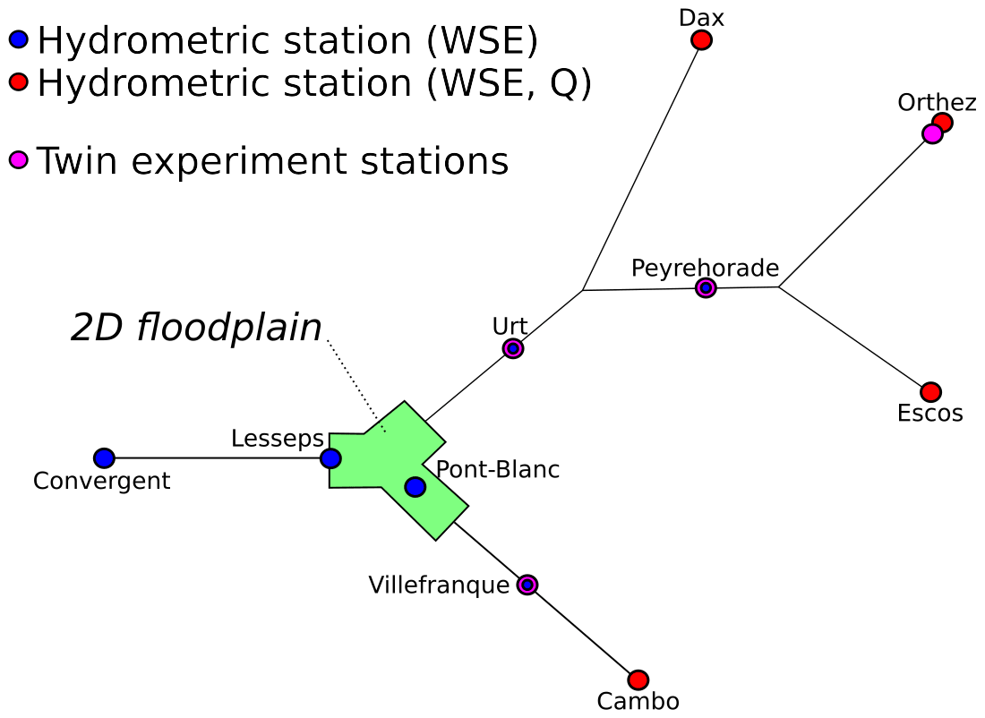
Figure 15Schematic view of the complete Adour River network and observability. Dimensions in the diagram are not to scale: total river lengths equal ≈180 km; 2D floodplain area equals . Tidal BC influence (from the downstream BC at Convergent) is observed up to Dax (and further upstream), Peyrehorade and Villefranque.
Model construction and rainfall to inundation simulation
The following model of the Adour River combines a multi-D hydraulic network model and several hydrological models of sub-catchments (Fig. 15). It encompasses around 180 km of river reaches and includes the Adour River from its tidal boundary downstream of Bayonne up to a gauging station around 70 km upstream and part of its main tributaries: the Nive River (around 45 km) and the Oloron and Pau rivers (around 65 km in total). The river network contains mostly single-branch reaches, with some notable flood areas around the city of Bayonne. The WS is observed in situ at 10 points, 5 of which are used as boundary conditions (Dax, Orthez, Escos, Cambo and Convergent in Fig. 15). Out of the five remaining stations kept for data assimilation, three are located on river reaches (Peyrehorade, Urt and Villefranque; blue points in Fig. 15) and two are located in the Bayonne area (Pont-Blanc and Lesseps; blue points in Fig. 15).
At the four upstream points of the modeled river network, four sub-catchments are modeled with four lumped hydrological models (Sect. 2.3). Their drainage areas are about 7811, 842, 2480 and 2464 km2. The hourly discharge has been extracted from the HYDRO2 database, while the rainfall data from the radar observation reanalysis ANTILOPE J+1, which merges radar and in situ gauge observations, is provided by Météo France. The interannual temperature data are provided by the SAFRAN reanalysis by Météo France and then used to calculate the potential evapotranspiration using the Oudin formula (Oudin et al., 2005). The rainfall and potential evapotranspiration are at a spatial resolution of a 1 km2 square grid and are processed at an hourly time step. Spatial averages of the rainfall and potential evapotranspiration computed using the SMASH distributed hydrological modeling platform (Jay-Allemand et al., 2020; Colleoni et al., 2021) over the four catchments are used as inputs for the lumped GR4H model. Lumped parameter sets for the four GR4H models are simply obtained here using for each the airGR global calibration algorithm (Coron et al., 2017). In this section, inferences are carried out only for upstream inflow hydrographs and not for hydrological parameters. Indeed, the study of global calibration and regionalization issues of spatially distributed hydrological models is left for further research.
Our multi-D hydraulic modeling approach (Sect. 2) is applied to this complex case as follows. First, a “1D-like-only” model of the whole network is built. Then, a multi-D model is built based on the 1D-like-only model, with the addition of a 2D mesh of a floodplain (Fig. 16a).
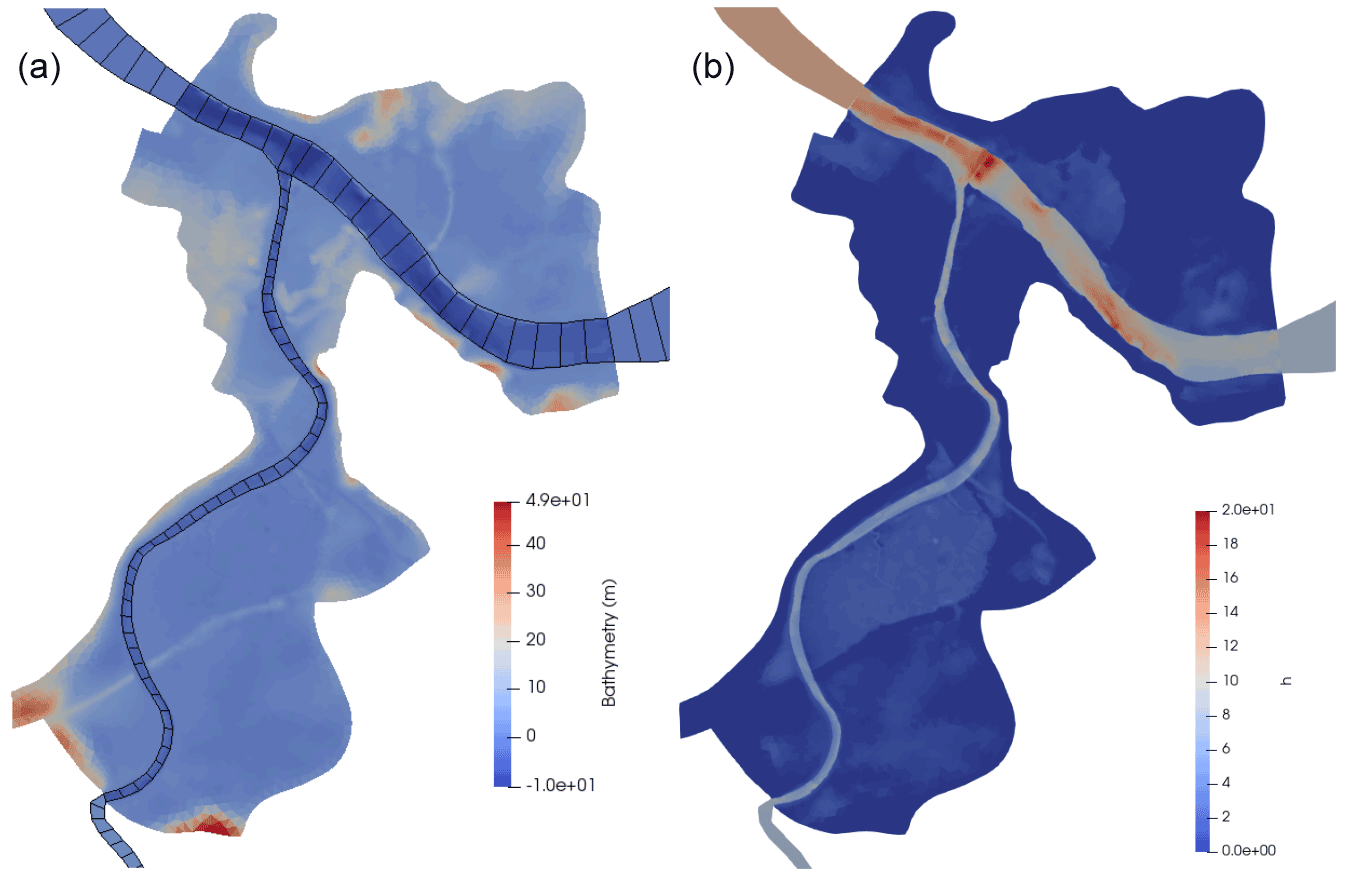
Figure 16Zoom on the Bayonne area (green area in Fig. 15) using the 1D-like and 1D–2D approaches. Manning values are homogeneous throughout the network and floodplains at . (a) Bathymetry in 1D-like and 2D meshes. The 2D area has 66 982 cells, and the coupled 1D-like reaches account for 1342 cells. The south, east and west interfaces, respectively, feature 6, 18 and 14 2D cells. The exclusively 1D-like mesh contains 1409 cells. (b) Simulated water height for the 1D–2D model for a sample flooding event (low tide, QAdour=650 m3 s−1 and QNive=58 m3 s−1 at 1D–2D interfaces).
On the 1D-like-only model, the goal is to analyze 1D-like signal propagation representation at a low computational cost. The Adour 1D-like model is built similarly to the Garonne 1D-like model, using DEM data to determine minor bed bank line placement and build the quadrangular cells. Bathymetry comes from 25×25 m DEM data, aggregated from fine lidar data from public databases, extracted at each cell. This rough approximation is sufficient to show the potential of the DassFlow assimilation tool chain for a large-scale river network. This 1D-like-only model contains 1409 cells. A 24 h simulation runs in around 13 s, using uncalibrated parameter estimates.
Then, a multi-D model is obtained: the existing 2D mesh from a Telemac model is coupled to a 1D-like mesh, similarly to the reference Telemac-Mascaret model from the regional flood forecast center SPC-GAD. The 1D-like parts of the mesh are kept identical to the 1D-like-only model, while the 2D part is the mesh extracted from the Telemac-Mascaret model (Fig. 16a) provided by SPC-GAD. For hydraulic coherence, bathymetry at coupled 1D-like cells is taken as the average bathymetry of the linked 2D cells. This 1D–2D model contains 66 982 cells in the 2D area and 1342 cells in 1D-like reaches. Results for a flooding event (around 6 h of computation per day, on a single thread ) in the Bayonne 2D area are presented in Fig. 16b. Modeled variables appear coherent over the 1D–2D area and a high-resolution flood map in coherence with flow conditions in the whole river network is obtained.
A 1 d (physical time) flooding event is computed in around 20 min (computation time) in the 1D–2D model (with 68 324 total cells, six threads in parallel). The same event leads to a 7 s computation time for the 1D-like-only model (with 1409 cells, same computational setup). Remember that computation time may vary depending on the number of wetted cells and on the adaptive time step calculation. This relatively low computation time and the potential to decrease it further by using more threads in parallel indicate that this multi-D method is suited to operational use. The code version this work is based on was proven to be scalable (Couderc et al., 2013). Additions made to the current version should not change this, but no numerical testing has been done.
Assimilation of WS observables to infer four upstream hydrographs
To investigate the 1D-like effective modeling on a river network, a twin experiment setup is designed to infer a large control vector from a realistic observability in the 1D-like-only model.
The considered control vector is composed of the four upstream hydrographs . Observations of WS elevation are generated at Peyrehorade, Urt and Villefranque stations and additionally at a virtual station directly downstream from Orthez. These four points give theoretically sufficient observability to identify the four upstream hydrographs. Indeed, they sample the mixed and unmixed signal similarly to the academic setup in Sect. 3.2.3. The observation pattern also corresponds to a reasonable expectation of spatial observability in French river networks. Prior hydrograph values are classically set to a constant average discharge value.
Simultaneous inference of the four hydrographs is satisfying. As shown in Fig. 17, left, upstream hydrographs injected at Cambo and Orthez are inferred very accurately (NSE >0.95). This is due to their WS elevation signature being observed to be unmixed in the respective downstream reaches. The Escos hydrograph WS signature is observed at Peyrehorade, mixed with the Orthez hydrograph WS elevation signature. This leads to a partial error of signature attribution and a less accurate inference (NSE =0.57). The Dax hydrograph WS elevation signature is observed only at the Urt station, where its signal is mixed with that of Escos and Orthez. The resulting inference is the less accurate, with a NSE of 0.50, and closer in shape to the inferred Escos and Orthez hydrographs. This suggests correlated influences of these hydrographs at observation stations and insufficient observability of the Dax hydrograph signal given the model hydrodynamics. Observed signals at the four stations are, however, all very accurate (Fig. 17, right). For upstream stations (Orthez and Villefranque), this is due to the accurate inference of upstream hydrographs. For stations under the influence of the tidal boundary condition (BC) (Peyrehorade and Urt), this is due to the backwater influence of the BC, which compensates for the error in inferred hydrographs (namely at Dax and less so at Escos).
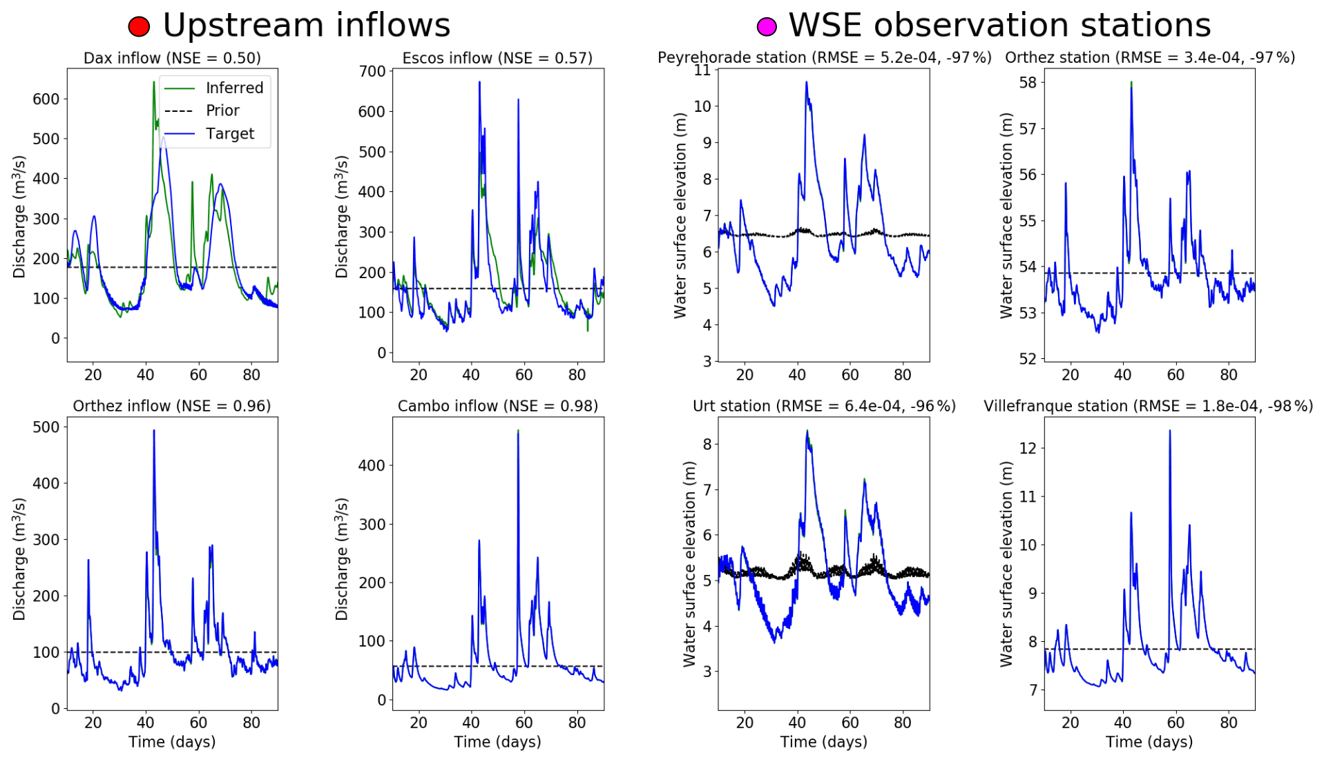
Figure 17Upstream hydrograph inferences from four observation stations in a twin experiment setup. Left: upstream inflow hydrographs used to generate observations (blue); inferred hydrographs at 20 iterations (green); background hydrograph value given for iteration 0 (mean target inflow over assimilation window; dotted lines). NSE values are given for their informative value but are not used in the assimilation process. Right: target WS elevation (blue); WS elevation generated by the inferred hydrographs (green); WS elevation generated by the background hydrographs (dotted lines). Downstream tidal boundary influence is felt at the two stations furthest downstream (Urt and Peyrehorade). RMSE values given are used to calculate cost in the assimilation process (Sect. 2.4).
In conclusion, this experiment shows the capability of the VDA tool chain to infer various upstream hydrographs in 1D-like network models. Note that multi-D models are identical to the investigated 1D-like model in terms of VDA capabilities. This paves the way towards investigations of multi-variate inferability of spatially distributed hydraulic–hydrological parameters.
In the future, investigation of the influence of data sparsity, observation weights and ill-posed problem constraints should be carried out.
This article presents a new approach and numerical chain for the multi-D hydrological–hydraulic modeling of complex river networks with variational data assimilation capabilities. It is based on the VDA algorithm and the finite-volume solvers (including a second-order one and accurate treatment of wet–dry front propagation) from Monnier et al. (2016). The resolution of the full 2D shallow-water equations (Eq. 1) is performed with a single finite-volume solver applied to a multi-D discretization of a river network domain. This lattice consists in 1D-like reaches meshed with irregular quadrangular cells connected via 1D-like–2D interfaces to 2D zooms consisting in higher-resolution unstructured meshes – either triangular or quadrangular. This hydraulic model with inflow from a hydrological model enabling us to describe upstream/lateral catchment inflow hydrographs. In this work, the parsimonious GR4 model is integrated (Perrin et al., 2003) in its state–space version (Santos et al., 2018) for the sake of differentiability (for the VDA computations). This approach is implemented in the platform DassFlow (Monnier et al., 2019). The adjoint of the whole tool chain is generated with Tapenade (Hascoet and Pascual, 2013) and validated. Forward-inverse capabilities with the new components are assessed in several cases of increasing complexity.
The 1D-like effective hydraulic modeling approach as well as its coupling with higher-resolution 2D zooms was validated, against (1) reference 1D and 2D hydraulic models, on an array of academic cases; (2) complex real cases featuring 1D and 2D flow variabilities in river networks with confluences and floodplains. These cases are also employed to test the coupling with the hydrological model implemented in a semi-distributed setup.
Considering single (multiple) type(s) of flow signature observations in those river networks through a single-objective (multi-objective) observation cost function, the capabilities of the VDA method for inferring mono- and/or multi-variate control vectors of large dimensions was successfully tested.
From the obtained results, the following conclusions can be drawn:
-
A complete integrated multi-D model coupled with an hydrological model has been implemented and validated in a parallel environment. Moreover, this complete tool chain includes VDA capabilities based on the adjoint code.
-
The 1D-like modeling approach enables us to simulate fine physical flow states compared to reference 1D or 2D SW models; hydrograph propagation remains very close also.
-
The inference, from heterogeneous observations in the river network, of multi-variate and high-dimension controls among multiple inflow discharge hydrographs, bathymetry, and friction of the full shallow-water multi-D hydraulic model but also hydrological model parameters is demonstrated. Very accurate inferences are obtained when the available information contained in system observability and priors is sufficient regarding the nature and quantity of unknown parameters (see discussion in Brisset et al., 2018, Larnier et al., 2020, Garambois et al., 2020, and references therein).
-
Information feedback from the river network to upstream hydrological models of sub-catchments is shown.
-
Real flows on complex channel geometries can be accurately simulated with the 1D-like model, despite its intrinsic rectangular XS, thanks to the calibration of effective geometry-friction patterns. The depth-dependent friction law helps to reduce misfits across flow regimes.
-
High-resolution simulations of real flows can be obtained on complex river networks including floodplains and confluences with reduced simulation costs.
To our knowledge, the present numerical tool is the first one proposing large-scale multi-D river network modeling with VDA capabilities. This new toolchain opens the way for the resolution of large-scale high-dimensional hydrological–hydraulic inverse problems that can be considered given constraints from multi-source datasets. The methods for direct and inverse modeling can be applied at multiple spatial scales including with a fine resolution (imposing finer calculation time steps to respect the Courant–Friedrichs–Lewy (CFL) condition in the forward hydraulic model). Building and constraining the models is, however, dependent on data availability and the informative content of observations, which may be linked to the spatial scale.
Short-term perspectives will aim to tailor the data assimilation algorithm to perform complex data assimilation experiments at basin scale using various multi-source datasets. To be actually operational, improvements pertaining to the construction of 1D-like models from global public databases are needed to deploy the multi-D approach to a large number of river networks. Coupling is ongoing with the SMASH spatially distributed hydrological platform (Jay-Allemand et al., 2020; Colleoni et al., 2021), on which the French flash flood warning system VigiCrues Flash (Garandeau et al., 2018) is based. Note that the addition of lateral flows (surface and subsurface runoff) would simply consist in imposing additional inflows on the boundary of the river/floodplain domain, which is numerically identical to the upstream flows imposed and inferred here (see such lateral coupling in 1D with inferences from sparse satellite altimetry data in Pujol et al., 2020). Further work will also test the integrated chain on Mediterranean basins at risk of flash flooding and on larger basins in a satellite observability context. The implementation of porosity models (Guinot et al., 2018, and references therein) represents a very interesting research direction regarding effective floodplains and 1D-like reach parameterizations. This is especially true with depth-dependent porosity (Özgen et al., 2017, and Guinot et al., 2018, and references therein) applied to complex channel geometries and with spatially distributed calibration.
A1 Two-dimensional solver
Recall the rotational invariance property of the SWE (Eq. 1), which simplifies the sum of 2D problems in Eq. (3) to 1D Riemann problems. The fluxes Fe are computed using a Riemann solver. Each local Riemann problem depends on left and right states at the interface e.
The Harten–Lax–van Leer condition (HLLC) approximate Riemann solver is used. This gives the following expressions:
where the wave speed expressions are those proposed in Vila (1986):
It has been demonstrated that this insures L∞ stability, positivity and consistency with the entropy condition under a CFL condition.
For the intermediate wave speed estimate, following Toro (2001), we set
A Courant–Friedrichs–Levy (CFL) condition for the time step Δtn applies; see, e.g., Vila and Villedieu (2003).
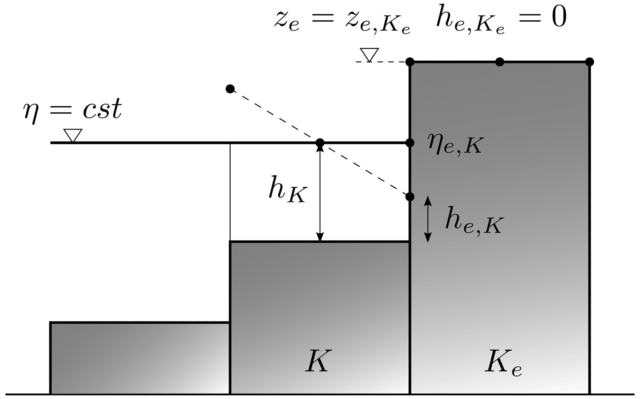
Figure A1Typical situation of desired well-balanced property in the presence of a wet–dry front. The WS elevation is here denoted by η.
A2 Well balancing
The numerical scheme must preserve the fluid at rest property; that is, the gradient of bathymetry ∇zb must not provide if un=0. In the presence of topography gradients (in particular those perpendicular to the streamlines) the basic topography gradient ∇zb discretization in the gravity source term Sg(U) generates spurious velocities. There is no discrete balance between the hydrostatic pressure and the gravity source term anymore: .
The technique which is employed here is that presented in Audusse et al. (2004) and Audusse and Bristeau (2005). It is based on the following change in variable.
From now, at the left and right sides of edge e, the considered water depth values are those defined from the “reconstructed” topography ze as
(see Fig. A1).
The conservative variable vector is now considered with the new variable:
Note that this new variable depends on the bathymetry values ze,K and ze.
The resulting scheme reads
with
This provides a well-balanced (first-order) scheme.
A3 Prediction-correction time scheme
The friction source term is taken into account in the complete SW system by deriving a prediction-correction time scheme; see, e.g., Toro (2001).
We denote here by the finite volume (FV) solution at time tn+1 of the (well-balanced) scheme, either first or second order, of the SW system with the gravitational term Sg but without the friction term Sf. Recall that we denote .
At each time step, from n to n+1, the following steps apply:
-
step 1: computation of , solution of the conservative SW system, i.e., the SW system without Sf, i.e., the FV solution of the following system:
-
step 2: given the ”predicted value” , compute Un+1 solution of
General schemes (explicit, implicit or semi-implicit ones) including the friction source term Sf in the discretization of the model (Eq. 1) for all K can be written as
Note that this splitting scheme is consistent at first order in Δt with the complete SWE. A splitting scheme of second order in time is possible; it is not detailed later.
In the case of the Manning–Strickler law, the friction term reads .
Therefore the equation to be solved (Eq. A9) reads
Since the friction source term Sf is zero in the mass conservation equation, we remark that . As a consequence, we consider the non-zero momentum component only: .
A4 First-order expression of Un+1
Let us consider the following implicit scheme:
This implies that
Let us set ; c≥0. Note that . Therefore for non-vanishing velocities, there exists such that . Adopting these notations, we obtain . This simplifies to
Since α≥0, the root of this quadratic equation reads
Let us define the function . Observe that ε=O(Δtn); also . By adopting this notation, Eq. (A15) reads . After some rearrangements, we obtain . At first order in ϵ, we get . Finally, we obtain
with the solution of Eq. (A8).
A5 Second-order MUSCL scheme
In order to obtain a globally second-order scheme, a higher-order time stepping scheme is needed. Let us briefly describe the ingredients of this second-order well-balanced positive scheme that is strictly the same as the one proposed in Couderc et al. (2013) and Monnier et al. (2016). Actual second-order accuracy, considering source terms Sg and Sf, is achieved through the combination of a Monotonic Upwind Scheme for Conservation Laws (MUSCL) spatial reconstruction and an IMEX RK time scheme (see Monnier et al., 2016, and references therein) as well as a spatial discretization of Sg and the semi-implicit nature of the friction source term Sf given in the subsection above.
A mono-slope second-order MUSCL scheme is adopted; see, e.g., Chévrier and Galley (1993) and Buffard and Clain (2010). It leads to new expressions of and . With this linear reconstruction, one can expect a scheme with a second-order accuracy in space (for regular solutions only). In order to prevent large numerical dispersive instabilities, the computed vectorial slopes are limited by applying a maximum principle. Furthermore, to handle the presence of wet–dry fronts that can break the finite-volume mass conservation property, a Barth limiter (Barth, 2003) is employed.
A river network Ω1D is described by connected closed line segments. For a flow XS orthogonal to the main (longitudinal) flow direction of curvilinear abscissa x∈Ω1D (distance from downstream areas) at time , let A(x,t) be the flow cross-sectional area [m2] and Q(x,t) the discharge [m3 s−1] such that Q=UA with U(x,t) defined as the longitudinal XS averaged velocity [m s−1]. The 1D Saint-Venant equations in the (A,Q) variables at a flow XS are written as follows:
where Z(x,t) is the WS elevation [m] and (with b(x) [m] the riverbed level and h(x,t) [m] the water depth), [m] the hydraulic radius, Ph(x,t) [m] the wetted perimeter, and g [m s−2] is the gravity magnitude. Let us recall the Froude number definition comparing the average flow velocity U to pressure wave celerity , where W [m] is the flow top width.
The friction term Sf is classically parameterized with the empirical Manning–Strickler law established for uniform flows , where K is the Strickler coefficient.
The Saint-Venant equations are solved on each segment of the river network and the continuity of the flow between segments is ensured by applying an equality constraint on water levels at the confluence between two segments.
Boundary conditions are classically imposed (subcritical flows here) at boundary nodes with inflow discharges Q(t) at upstream nodes and WS elevation Z(t) at the downstream node; there are lateral hydrographs ql(t) at in/outflow nodes. The initial condition is set as the steady-state backwater curve profile for a hot start. This 1D Saint-Venant model is discretized using the classical implicit Preissmann scheme (see, e.g., Cunge et al., 1980) on a regular grid of spacing Δx using a double sweep method enabling us to deal with flow regimes changes with a 1 h time step Δt. This is implemented in the computational software DassFlow (Brisset et al., 2018; Larnier, 2010).
The numerical scheme is a semi-implicit finite-difference scheme (generalized Preissmann scheme) with a double sweep Local Partial Inertial method to minimize the inertial terms (see documentation in Brisset et al., 2018, and Larnier, 2010).
The state–space version of the lumped conceptual hydrological model GR4 presented in Santos et al. (2018) consists in the set of ODEs below:
They involve the following fluxes:
The following parameters are set following Perrin et al. (2003) and Santos et al. (2018): α=2, β=5, γ=5, ω=3.5, , Φ=0.9, nres=11.
Calibrated parameters for the Adour case were obtained using the airGR global calibration algorithm (Coron et al., 2017) from the freely available package (https://webgr.inrae.fr/logiciels/airgr/, last access: 27 July 2022).
Table C1Calibrated hydrological parameters of the four upstream hydrological catchments from the Adour multi-D hydrographic network model.
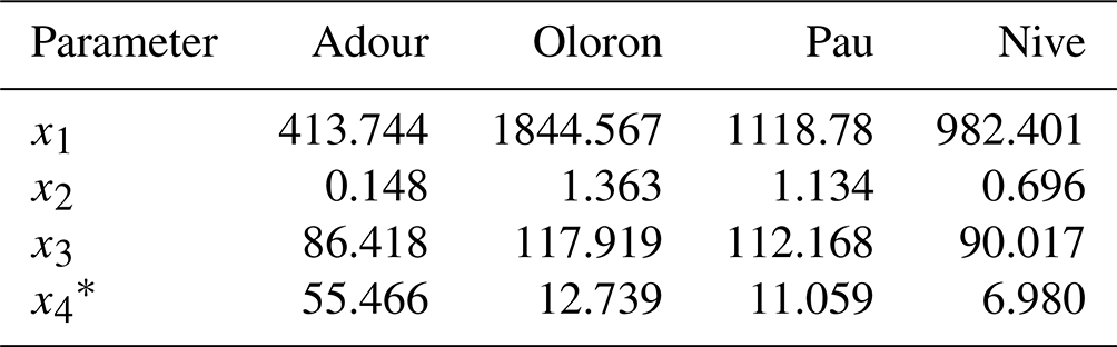
∗ Note that the x4 calibrated parameter corresponds to the non-“state–space” GR4H version (not presented, see Perrin et al., 2003), for which the calibration tool is provided. x4 values in the present run with the state–space were set at 0.15.
The current DassFlow code is available on demand at https://www.math.univ-toulouse.fr/DassFlow/download.html (last access: 27 July 2022). The exact version of the model used in this article is archived on Zenodo (https://doi.org/10.5281/zenodo.6342723, Pujol et al., 2022), as are input data needed to run the main direct/inverse simulations.
This work is part of the PhD work of LP under the supervision of PAG and JM. The research plan was developed by PAG, LP and JM. The computational software DassFlow2D was adapted from a previous version by LP under the supervision of PAG and JM. Numerical investigations were carried out by LP with analyses by all. JM designed or supervised the 2D numerical scheme and VDA algorithm. PAG and JM designed and co-supervised the 1D–2D algorithm. All authors participated in the writing. PAG was responsible for the project management for funding.
The contact author has declared that none of the authors has any competing interests.
Publisher’s note: Copernicus Publications remains neutral with regard to jurisdictional claims in published maps and institutional affiliations.
This study was rendered possible by the adaptation of covariance matrices in the inverse algorithm from the DassFlow1D algorithm (Larnier et al., 2020) by Lilian Villenave (INRAE Aix-en-Provence) and the implementation of final tricks in Perl scripts for adjoint post-processing in DassFlow by Kévin Larnier (CS Group Toulouse). The authors greatly acknowledge Pascal Finaud-Guyot (HydroSciences, University of Montpellier) for fruitful discussions related to hydraulic solvers. They warmly thank Laurent Dieval from SPC-GAD France, the operational flood forecasting service for the Gaves–Adour–Dordogne river networks, for providing data for the Adour case and also for interesting discussions. They also thank Robert Mosé (ICUBE, University of Strasbourg), the PhD director of Léo Pujol.
Léo Pujol has been co-funded by CNES and ICUBE.
This paper was edited by Charles Onyutha and reviewed by two anonymous referees.
Allen, M., Antwi-Agyei, P., Aragon-Durand, F., Babiker, M., Bertoldi, P., Bind, M., Brown, S., Buckeridge, M., Camilloni, I., Cartwright, A., Masson-Delmotte, V., Zhai, P., Pörtner, H.-O., Roberts, D., Skea, J., Shukla, P. R., Pirani, A., Moufouma-Okia, W., Péan, C., Pidcock, R., Connors, S., Matthews, J. B. R., Chen, Y., Zhou, X., Gomis, M. I., Lonnoy, E., Maycock, T., Tignor, M., and Waterterfield, T. (Eds.): Technical Summary: Global warming of 1.5 ∘C, An IPCC Special Report on the impacts of global warming of 1.5 ∘C above pre-industrial levels and related global greenhouse gas emission pathways, in the context of strengthening the global response to the threat of climate change, sustainable development, and efforts to eradicate poverty, http://pure.iiasa.ac.at/15716 (last access: 27 June 2022), 2019. a
Amara, M., Capatina-Papaghiuc, D., and Trujillo, D.: Hydrodynamical modelling and multidimensional approximation of estuarian river flows, Comput. Vis. Sci., 6, 39–46, https://doi.org/10.1007/s00791-003-0106-z, 2004. a
Asch, M., Bocquet, M., and Nodet, M.: Data assimilation: methods, algorithms, and applications, Fundamentals of Algorithms, SIAM, https://hal.inria.fr/hal-01402885 (last access: 27 June 2022), 2016. a
Audusse, E. and Bristeau, M.-O.: A well-balanced positivity preserving “second-order” scheme for shallow water flows on unstructured meshes, J. Comput. Phys., 206, 311–333, https://doi.org/10.1016/j.jcp.2004.12.016, 2005. a
Audusse, E., Bouchut, F., Bristeau, M.-O., Klein, R., and Perthame, B.: A Fast and Stable Well-Balanced Scheme with Hydrostatic Reconstruction for Shallow Water Flows, SIAM J. Sci. Comput., 25, 2050–2065, https://doi.org/10.1137/S1064827503431090, 2004. a
Barth, T.: Numerical Methods for conservative Laws on Structured and Unstructured Meshes, Tech. rep., VKI Lecture Series, 2003. a
Barthélémy, S., Ricci, S., Morel, T., Goutal, N., Le Pape, E., and Zaoui, F.: On operational flood forecasting system involving 1D2D coupled hydraulic model and data assimilation, J. Hydrol., 562, 623–634, https://doi.org/10.1016/j.jhydrol.2018.05.007, 2018. a
Bates, P., Trigg, M., Neal, J., and Dabrowa, A.: LISFLOOD-FP, User manual, School of Geographical Sciences, University of Bristol, Bristol, UK, https://vdocument.in/lisflood-fp-user-manual-university-of-bristol (last access: 1 August 2022), 2013. a
Bates, P. D., Horritt, M. S., and Fewtrell, T. J.: A simple inertial formulation of the shallow water equations for efficient two-dimensional flood inundation modelling, J. Hydrol., 387, 33–45, https://doi.org/10.1016/j.jhydrol.2010.03.027, 2010. a
Bertalanffy, L. v.: General Systems Theory, 1968. a
Beven, K.: Prophecy, reality and uncertainty in distributed hydrological modelling, Adv. Water Resour., 16, 41–51, 1993. a
Beven, K. J.: Uniqueness of place and process representations in hydrological modelling, Hydrol. Earth Syst. Sci., 4, 203–213, https://doi.org/10.5194/hess-4-203-2000, 2000. a
Biancamaria, S., Lettenmaier, D., and Pavelsky, T.: The SWOT Mission and Its Capabilities for Land Hydrology, Surv. Geophys., 37, 307–337, https://doi.org/10.1007/s10712-015-9346-y, 2016. a
Biancamaria, S., Frappart, F., Leleu, A.-S., Marieu, V., Blumstein, D., Desjonquères, J.-D., Boy, F., Sottolichio, A., and Valle-Levinson, A.: Satellite radar altimetry water elevations performance over a 200 m wide river: Evaluation over the Garonne River, Adv. Space Res., 59, 128–146, https://doi.org/10.1016/j.asr.2016.10.008, 2017. a
Bouttier, F. and Courtier, P.: Data assimilation concepts and methods March 1999, Meteorological training course lecture series, ECMWF, 718, 59, http://msi.ttu.ee/~elken/Assim_concepts.pdf (last access: 27 June 2022), 2002. a, b
Brêda, J., Paiva, R., Bravo, J., Passaia, O., and Moreira, D.: Assimilation of satellite altimetry data for effective river bathymetry, Water Resour. Res., 55, 7441–7463, https://doi.org/10.1029/2018WR024010, 2019. a
Brisset, P., Monnier, J., Garambois, P.-A., and Roux, H.: On the assimilation of altimetric data in 1D Saint-Venant river flow models, Adv. Water Res., 119, 41–59, https://doi.org/10.1016/j.advwatres.2018.06.004, 2018. a, b, c, d, e, f, g, h, i, j, k
Brunner, G. W.: HEC-RAS River Analysis System, Hydraulic Reference Manual, Version 1.0., Tech. rep., Hydrologic Engineering Center Davis, CA, https://apps.dtic.mil/sti/pdfs/ADA311952.pdf (last access: 27 June 2022) 1995. a
Buffard, T. and Clain, S.: Monoslope and Multislope MUSCL Methods for unstructured meshes, J. Comput. Phys., 229, 3745–3776, https://doi.org/10.1016/j.jcp.2010.01.026, 2010. a
Chévrier, P. and Galley, H.: A Van Leer finite volume scheme for the Euler equations on unstructured meshes, ESAIM-Math. Model. Num., 27, 183–201, 1993. a
Chow, V.: Open-channel Hydraulics, McGraw-Hill civil engineering series, McGraw-Hill, New-York, USA, ISBN 9780070859067, 1959. a
Colleoni, F., Garambois, P.-A., Javelle, P., Jay-Allemand, M., I., G., Organde, D., and Arnaud, P.: SMASH v1.0 platform for spatially distributed hydrological modeling and data assimilation: hypothesis testing and signatures analysis, J. Hydrol., submitted, 2021. a, b
Collischonn, W., Allasia, D., Da Silva, B. C., and Tucci, C. E.: The MGB-IPH model for large-scale rainfall-runoff modelling, Hydrolog. Sci. J., 52, 878–895, https://doi.org/10.1623/hysj.52.5.878, 2007. a
Coron, L., Thirel, G., Delaigue, O., Perrin, C., and Andréassian, V.: The suite of lumped GR hydrological models in an R package, Environ. Modell. Softw., 94, 166–171, https://doi.org/10.1016/j.envsoft.2017.05.002, 2017. a, b
Couderc, F., Madec, R., Monnier, J., and Vila, J.-P.: DassFow-Shallow, Variational Data Assimilation for Shallow-Water Models: Numerical Schemes, User and Developer Guides, University of Toulouse, CNRS, IMT, INSA, ANR, Research report, https://hal.archives-ouvertes.fr/hal-01120285 (last access: 27 June 2022), 2013. a, b, c, d, e
Cunge, J. A., Holly, F., M., and Verwey, A.: Practical Aspects of Computational River Hydraulics, Pitam Publishing, ISBN 978-0273084426, 1980. a
Davy, P., Croissant, T., and Lague, D.: A precipiton method to calculate river hydrodynamics, with applications to flood prediction, landscape evolution models, and braiding instabilities, J. Geophys. Res.-Earth, 122, 1491–1512, https://doi.org/10.1002/2016JF004156, 2017. a, b
Delestre, O., Darboux, F., James, F., Lucas, C., Laguerre, C., and Cordier, S.: FullSWOF: Full Shallow-Water equations for Overland Flow, J. Open Source Softw., 2, 448, https://doi.org/10.21105/joss.00448, 2017. a
Dingman, S. L.: Fluvial hydraulics, Oxford University Press, ISBN 978-0-19-517286-7, 2009. a, b
Finaud-Guyot, P., Garambois, P.-A., Chen, S., Dellinger, G., Ghenaim, A., and Terfous, A.: 1D2D porosity model for urban flood modeling: case of a dense street networks, E3S Web Conf., 40, 06010, https://doi.org/10.1051/e3sconf/20184006010, 2018. a
Fleischmann, A. S., Paiva, R. C. D., Collischonn, W., Siqueira, V. A., Paris, A., Moreira, D. M., Papa, F., Bitar, A. A., Parrens, M., Aires, F., and Garambois, P. A.: Trade-offs between 1-D and 2-D regional river hydrodynamic models, Water Resour. Res., 56, e2019WR026812, https://doi.org/10.1029/2019WR026812, 2020. a, b, c
Galland, J.-C., Goutal, N., and Hervouet, J.-M.: TELEMAC: A new numerical model for solving shallow water equations, Adv. Water Resour., 14, 138–148, 1991. a
Garambois, P., Calmant, S., Roux, H., Paris, A., Monnier, J., Finaud-Guyot, P., Montazem, A., and da Silva, J.: Hydraulic visibility: Using satellite altimetry to parameterize a hydraulic model of an ungauged reach of a braided river, Hydrol. Process., 31, 756–767, https://doi.org/10.1002/hyp.11033, 2017. a, b
Garambois, P.-A. and Monnier, J.: Inference of effective river properties from remotely sensed observations of water surface, Adv. Water Resour., 79, 103–120, https://doi.org/10.1016/j.advwatres.2015.02.007, 2015. a, b
Garambois, P.-A., Larnier, K., Monnier, J., Finaud-Guyot, P., Verley, J., Montazem, A., and Calmant, S.: Variational estimation of effective channel and ungauged anabranching river discharge from multi-satellite water heights of different spatial sparsity, J. Hydrol., 581, 124409, https://doi.org/10.1016/j.jhydrol.2019.124409, 2020. a, b, c, d
Garandeau, L., Belleudy, A., Javelle, P., Organde, D., Janet, B., Demargne, J., De Saint-Aubin, C., and Fouchier, C.: Vigicrues Flash, un service automatique d'avertissement pour les crues rapides, De la prévision des crues à la gestion de crise, Société Hydrotechnique de France, Avignon, France, 11, https://hal.inrae.fr/hal-02608801 (last access: 27 June 2022), 2018. a
Gejadze, I. Y. and Monnier, J.: On a 2D zoom for the 1D shallow water model: Coupling and data assimilation, Comput. Method. Appl. M., 196, 4628–4643, https://doi.org/10.1016/j.cma.2007.05.026, 2007. a
Gervasio, P., Lions, J.-L., and Quarteroni, A.: Heterogeneous coupling by virtual control methods, Numer. Math., 90, 241–264, https://doi.org/10.1007/s002110100303, 2001. a
Goutal, N. and Maurel, F.: A finite volume solver for 1D shallow-water equations applied to an actual river, Int. J. Numer. Meth. Fl., 38, 1–19, https://doi.org/10.1002/fld.201, 2002. a
Grimaldi, S., Li, Y., Walker, J., and Pauwels, V.: Effective representation of river geometry in hydraulic flood forecast models, Water Resour. Res., 54, 1031–1057, https://doi.org/10.1002/2017WR021765, 2018. a, b
Gudmundsson, G. H.: Transmission of basal variability to a glacier surface, J. Geophys. Res.-Sol. Ea., 108, B5, https://doi.org/10.1029/2002JB002107, 2003. a
Guinot, V.: Wave propagation in fluids: models and numerical techniques, 2nd edn., vol. 49, edited by: ISTE Ltd., ISBN 978-9812707789, 2010. a
Guinot, V., Delenne, C., Rousseau, A., and Boutron, O.: Flux closures and source term models for shallow water models with depth-dependent integral porosity, Adv. Water Resour., 122, 1–26, https://doi.org/10.1016/j.advwatres.2018.09.014, 2018. a, b, c
Hascoet, L. and Pascual, V.: The Tapenade automatic differentiation tool: principles, model, and specification, ACM T. Math. Software, 39, 1–43, https://doi.org/10.1145/2450153.2450158, 2013. a, b, c, d
Hocini, N., Payrastre, O., Bourgin, F., Gaume, E., Davy, P., Lague, D., Poinsignon, L., and Pons, F.: Performance of automated methods for flash flood inundation mapping: a comparison of a digital terrain model (DTM) filling and two hydrodynamic methods, Hydrol. Earth Syst. Sci., 25, 2979–2995, https://doi.org/10.5194/hess-25-2979-2021, 2021. a, b, c
Hostache, R., Lai, X., Monnier, J., and Puech, C.: Assimilation of spatially distributed water levels into a shallow-water flood model. Part II: Use of a remote sensing image of Mosel River, J. Hydrol., 390, 257–268, https://doi.org/10.1016/j.jhydrol.2010.07.003, 2010. a
Hunter, N. M., Bates, P. D., Neelz, S., Pender, G., Villanueva, I., Wright, N. G., Liang, D., Falconer, R. A., Lin, B., Waller, S., Crossley, A. J., and Mason, D. C.: Benchmarking 2D hydraulic models for urban flooding, in: Proceedings of the Institution of Civil Engineers-Water Management, Thomas Telford Ltd, 161, 13–30, https://doi.org/10.1680/wama.2008.161.1.13, 2008. a
Iturbide, M., Gutiérrez, J. M., Alves, L. M., Bedia, J., Cerezo-Mota, R., Cimadevilla, E., Cofiño, A. S., Di Luca, A., Faria, S. H., Gorodetskaya, I. V., Hauser, M., Herrera, S., Hennessy, K., Hewitt, H. T., Jones, R. G., Krakovska, S., Manzanas, R., Martínez-Castro, D., Narisma, G. T., Nurhati, I. S., Pinto, I., Seneviratne, S. I., van den Hurk, B., and Vera, C. S.: An update of IPCC climate reference regions for subcontinental analysis of climate model data: definition and aggregated datasets, Earth Syst. Sci. Data, 12, 2959–2970, https://doi.org/10.5194/essd-12-2959-2020, 2020. a
Jay-Allemand, M., Javelle, P., Gejadze, I., Arnaud, P., Malaterre, P.-O., Fine, J.-A., and Organde, D.: On the potential of variational calibration for a fully distributed hydrological model: application on a Mediterranean catchment, Hydrol. Earth Syst. Sci., 24, 5519–5538, https://doi.org/10.5194/hess-24-5519-2020, 2020. a, b
Kirstetter, G., Delestre, O., Lagrée, P.-Y., Popinet, S., and Josserand, C.: B-flood 1.0: an open-source Saint-Venant model for flash-flood simulation using adaptive refinement, Geosci. Model Dev., 14, 7117–7132, https://doi.org/10.5194/gmd-14-7117-2021, 2021. a
Lai, X. and Monnier, J.: Assimilation of spatially distributed water levels into a shallow-water flood model. Part I: Mathematical method and test case, J. Hydrol., 377, 1–11, https://doi.org/10.1016/j.jhydrol.2009.07.058, 2009. a
Larnier, K.: Modélisation thermohydraulique d'un troncon de Garonne en lien avec l'habitat piscicole: Approches statistique et déterministe, PhD thesis, Institut National Polytechnique de Toulouse, http://ethesis.inp-toulouse.fr/archive/00001263/ (last access: 27 June 2022), 2010. a, b
Larnier, K., Monnier, J., Garambois, P.-A., and Verley, J.: River discharge and bathymetry estimation from SWOT altimetry measurements, Inverse Probl. Sci. Eng., 29, 759–789, https://doi.org/10.1080/17415977.2020.1803858, 2020. a, b, c, d, e, f, g, h, i, j, k, l, m
Le Lay, M.: Modélisation hydrologique dans un contexte de variabilité hydro-climatique. Une approche comparative pour l'étude du cycle hydrologique à méso-échelle au Bénin, PhD thesis, Institut National Polytechnique de Grenoble (INPG), https://tel.archives-ouvertes.fr/tel-00116912 (last access: 27 June 2022), 2006. a
Leopold, L. B. and Maddock, T.: The hydraulic geometry of stream channels and some physiographic implications, US Government Printing Office, 252, https://doi.org/10.3133/pp252, 1953. a
Lorenc, A. C., Ballard, S. P., Bell, R. S., Ingleby, N. B., Andrews, P. L. F., Barker, D. M., Bray, J. R., Clayton, A. M., Dalby, T., Li, D., Payne, T. J., and Saunders, F. W.: The Met. Office global three-dimensional variational data assimilation scheme, Q. J. Roy. Meteor. Soc., 126, 2991–3012, 2000. a
Malou, T. and Monnier, J.: Double-scale diffusive wave model dedicated to spatial river observation and associated covariance kernel for variational data assimilation , EGU General Assembly 2021, online, 19–30 Apr 2021, EGU21-10355, https://doi.org/10.5194/egusphere-egu21-10355, 2021. a
Malou, T. and Monnier, J.: Covariance kernels investigation from diffusive wave equations for data assimilation in hydrology, Inverse Probl., https://doi.org/10.1088/1361-6420/ac509d, accepted, 2022. a
Malou, T., Garambois, P.-A., Paris, A., Monnier, J., and Larnier, K.: Generation and analysis of stage-fall-discharge laws from coupled hydrological-hydraulic river network model integrating sparse multi-satellite data, J. Hydrol., 603, 126993, https://doi.org/10.1016/j.jhydrol.2021.126993, 2021. a, b, c
Marin, J. and Monnier, J.: Superposition of local zoom models and simultaneous calibration for 1D–2D shallow water flows, Math. Comput. Simulat., 80, 547–560, https://doi.org/10.1016/j.matcom.2009.09.001, 2009. a
Martin, N. and Monnier, J.: Inverse rheometry and basal properties inference for pseudoplastic geophysical flows, Eur. J. Mech. B-Fluid., 50, 110–126, https://doi.org/10.1016/j.euromechflu.2014.11.011, 2015. a
Miglio, E., Perotto, S., and Saleri, F.: Model coupling techniques for free-surface flow problems: Part I, Nonlinear Anal.-Theor., 63, e1885–e1896, https://doi.org/10.1016/j.na.2005.03.083, 2005a. a
Miglio, E., Perotto, S., and Saleri, F.: Model coupling techniques for free-surface flow problems: Part II, Nonlinear Anal.-Theor., 63, e1897–e1908, https://doi.org/10.1016/j.na.2005.03.085, 2005b. a
Milly, P.: Climate, soil water storage, and the average annual water balance, Water Resour. Res., 30, 2143–2156, https://doi.org/10.1029/94WR00586, 1994. a
Monnier, J.: Variational data assimilation: from optimal control to large scale data assimilation, Open Online Course, INSA Toulouse, https://www.math.univ-toulouse.fr/~jmonnie/Enseignement/CourseVDA.pdf (last access: 27 June 2022), 2014. a
Monnier, J.: Variational Data Assimilation and Model Learning, https://hal.archives-ouvertes.fr/hal-03040047 (last access: 1 August 2022), 2021. a
Monnier, J., Couderc, F., Dartus, D., Larnier, K., Madec, R., and Vila, J.-P.: Inverse algorithms for 2D shallow water equations in presence of wet dry fronts: Application to flood plain dynamics, Adv. Water Resour., 97, 11–24, https://doi.org/10.1016/j.advwatres.2016.07.005, 2016. a, b, c, d, e, f, g, h, i, j, k, l, m, n, o, p, q
Monnier, J., Couderc, F., and Vila, J.-P.: Data Assimilation for Free Surface Flows, Mathematics Institute of Toulouse – INSA corp. CNES-CNRS, Tech. rep., http://www.math.univ-toulouse.fr/DassFlow (last access: 27 June 2022), 2019. a, b, c
Montazem, A., Garambois, P.-A., Calmant, S., Finaud-Guyot, P., Monnier, J., Moreira, D., Minear, J., and Biancamaria, S.: Wavelet-Based River Segmentation Using Hydraulic Control-Preserving Water Surface Elevation Profile Properties, Geophys. Res. Lett., 46, 6534–6543, https://doi.org/10.1029/2019GL082986, 2019. a, b, c
Nguyen, P., Thorstensen, A., Sorooshian, S., Hsu, K., AghaKouchak, A., Sanders, B., Koren, V., Cui, Z., and Smith, M.: A high resolution coupled hydrologic-hydraulic model (HiResFlood-UCI) for flash flood modeling, J. Hydrol., 541, 401–420, https://doi.org/10.1016/j.jhydrol.2015.10.047, 2016. a, b, c
Oudin, L., Hervieu, F., Michel, C., Perrin, C., Andréassian, V., Anctil, F., and Loumagne, C.: Which potential evapotranspiration input for a lumped rainfall-runoff model?: Part 2 Towards a simple and efficient potential evapotranspiration model for rainfall-runoff modelling, J. Hydrol., 303, 290–306, https://doi.org/10.1016/j.jhydrol.2004.08.026, 2005. a
Özgen, I., Zhao, J.-h., Liang, D.-f., and Hinkelmann, R.: Wave propagation speeds and source term influences in single and integral porosity shallow water equations, Water Sci. Eng., 10, 275–286, https://doi.org/10.1016/j.wse.2017.12.003, 2017. a
Perrin, C., Michel, C., and Andréassian, V.: Improvement of a parsimonious model for streamflow simulation, J. Hydrol., 279, 275–289, https://doi.org/10.1016/S0022-1694(03)00225-7, 2003. a, b, c, d, e, f, g
Pontes, P., Fan, F., Fleischmann, A., Paiva, R., Buarque, D., Siqueira, V., Jardim, P., Sorribas, M., and Collischonn, W.: MGB-IPH model for hydrological and hydraulic simulation of large floodplain river systems coupled with open source GIS, Environ. Modell. Softw., 94, 1–20, https://doi.org/10.1016/j.envsoft.2017.03.029, 2017. a
Pujol, L., Garambois, P.-A., Finaud-Guyot, P., Monnier, J., Larnier, K., Mosé, R., Biancamaria, S., Yesou, H., Moreira, D., Paris, A., and Calmant, S.: Estimation of multiple inflows and effective channel by assimilation of multi-satellite hydraulic signatures: The ungauged anabranching Negro river, J. Hydrol., 591, 125331, https://doi.org/10.1016/j.jhydrol.2020.125331, 2020. a, b, c, d, e, f, g, h, i
Pujol, L., Garambois, P.-A., and Monnier, J.: DassFlow2D-V3 code and cases, Zenodo [code], https://doi.org/10.5281/zenodo.6342723, 2022. a, b
Rodríguez, E., Durand, M., and Frasson, R. P. d. M.: Observing rivers with varying spatial scales, Water Resour. Res., 56, 9, https://doi.org/10.1029/2019WR026476, 2020. a
Sanders, B. F., Schubert, J. E., and Detwiler, R. L.: ParBreZo: A parallel, unstructured grid, Godunov-type, shallow-water code for high-resolution flood inundation modeling at the regional scale, Adv. Water Resour., 33, 1456–1467, https://doi.org/10.1016/j.advwatres.2010.07.007, 2010. a, b
Santos, L., Thirel, G., and Perrin, C.: Continuous state-space representation of a bucket-type rainfall-runoff model: a case study with the GR4 model using state-space GR4 (version 1.0), Geosci. Model Dev., 11, 1591–1605, https://doi.org/10.5194/gmd-11-1591-2018, 2018. a, b, c, d, e, f, g, h
Schuite, J., Flipo, N., Massei, N., Rivière, A., and Baratelli, F.: Improving the Spectral Analysis of Hydrological Signals to Efficiently Constrain Watershed Properties, Water Resour. Res., 55, 4043–4065, https://doi.org/10.1029/2018WR024579, 2019. a
Schumann, G. J.-P. and Domeneghetti, A.: Exploiting the proliferation of current and future satellite observations of rivers, Hydrol. Process., 30, 2891–2896, https://doi.org/10.1002/hyp.10825, 2016. a
Steinstraesser, J. G. C., Delenne, C., Finaud-Guyot, P., Guinot, V., Casapia, J. K., and Rousseau, A.: SW2D-LEMON: a new software for upscaled shallow water modeling, in: Simhydro 2021 – 6th International Conference Models for complex and global water issues-Practices and expectations, Sophia Antipolis, 16–18 June 2021, https://hal.inria.fr/hal-03224050/ (last access: 27 June 2022), 2021. a
Toro, E.: Shock-capturing methods for free-surface shallow flows, Wiley Blackwell, ISBN 978-0-471-98766-6, 2001. a, b
Uhe, P., Mitchell, D., Bates, P. D., Addor, N., Neal, J., and Beck, H. E.: Model cascade from meteorological drivers to river flood hazard: flood-cascade v1.0, Geosci. Model Dev., 14, 4865–4890, https://doi.org/10.5194/gmd-14-4865-2021, 2021. a, b
Vila, J.-P.: Simplified Godunov schemes for 2×2 systems of conservation laws, SIAM J. Numer. Anal., 23, 1173–1192, https://doi.org/10.1137/0723079, 1986. a
Vila, J.-P. and Villedieu, P.: Convergence of an explicit finite volume scheme for first order symmetric systems, Numer. Math., 94, 573–602, https://doi.org/10.1007/s00211-002-0396-y, 2003. a
Zhu, C., Byrd, R. H., Lu, P., and Nocedal, J.: Algorithm 778: L-BFGS-B: Fortran subroutines for large-scale bound-constrained optimization, ACM T. Math. Software, 23, 550–560, https://doi.org/10.1145/279232.279236, 1997. a, b, c
https://www.aquaveo.com/software (last access: 27 June 2022); a software including comprehensive meshing tools.
http://www.hydro.eaufrance.fr (last access: 27 June 2022); Office français pour la biodiversité.
- Abstract
- Introduction
- The computational hydrological–hydraulic chain
- Results and discussion
- Conclusions and perspectives
- Appendix A: 2D shallow-water scheme
- Appendix B: 1D (A,Q) Saint-Venant
- Appendix C: GR4 hydrological model operators
- Code and data availability
- Author contributions
- Competing interests
- Disclaimer
- Acknowledgements
- Financial support
- Review statement
- References