the Creative Commons Attribution 4.0 License.
the Creative Commons Attribution 4.0 License.
 | 03 Aug 2022
A daily highest air temperature estimation method and spatial–temporal changes analysis of high temperature in China from 1979 to 2018
Ping Wang
Fei Meng
Zhihao Qin
Sayed M. Bateni
The daily highest air temperature (Tmax) is a key parameter for global and regional high temperature analysis which is very difficult to obtain in areas where there are no meteorological observation stations. This study proposes an estimation framework for obtaining high-precision Tmax. Firstly, we build a near-surface air temperature diurnal variation model to estimate Tmax with a spatial resolution of 0.1∘ for China from 1979 to 2018 based on multi-source data. Then, in order to further improve the estimation accuracy, we divided China into six regions according to climate conditions and topography and established calibration models for different regions. The analysis shows that the mean absolute error (MAE) of the dataset (https://doi.org/10.5281/zenodo.6322881, Wang et al., 2021) after correction with the calibration models is about 1.07 ∘C and the root mean square error (RMSE) is about 1.52 ∘C, which is higher than that before correction to nearly 1 ∘C. The spatial–temporal variations analysis of Tmax in China indicated that the annual and seasonal mean Tmax in most areas of China showed an increasing trend. In summer and autumn, the Tmax in northeast China increased the fastest among the six regions, which was 0.4∘C per 10 years and 0.39∘C per 10 years, respectively. The number of summer days and warm days showed an increasing trend in all regions while the number of icing days and cold days showed a decreasing trend. The abnormal temperature changes mainly occurred in El Niño years or La Niña years. We found that the influence of the Indian Ocean basin warming (IOBW) on air temperature in China was generally greater than those of the North Atlantic Oscillation and the NINO3.4 area sea surface temperature after making analysis of ocean climate modal indices with air temperature. In general, this Tmax dataset and analysis are of great significance to the study of climate change in China, especially for environmental protection.
- Article
(27377 KB) - Full-text XML
- BibTeX
- EndNote


In the context of global warming, the frequency of high-temperature events is increasing and high temperature tends to increase electricity demand and energy consumption (Zhang et al., 2021; Sathaye et al., 2013), adversely affecting human health, social economy and ecosystem (Sehra et al., 2020; Basu, 2009; Gasparrini and Armstrong, 2011). The daily highest air temperature (Tmax) is the basic parameter for studying regional-scale high-temperature events. It has a great influence on the ozone concentration (Abdullah et al., 2017; Kleinert et al., 2021) and the start time of the plant growth season on the Tibetan Plateau (Yang et al., 2017). Tmax is not only an important factor for high temperature disaster risk assessment but also a key input parameter for crop growth models and carbon emission models. Sustained and abnormally high Tmax will cause high temperature heat damage and adversely affect crop growth. Therefore, it is very important to accurately obtain the temporal and spatial distribution of Tmax and study the characteristics of high temperature weather. Generally, Tmax is measured on a thermometer in a louvered box 1.5 m above the ground in the field. However, the Tmax measured by this method has high accuracy but not spatial continuity. Therefore, some scholars spatialized the station-based Tmax through methods such as Kriging interpolation and spline function interpolation. However, the number of meteorological stations is limited, and stations in remote areas and areas with complex terrain are even sparser which makes the accuracy of Tmax obtained by interpolation difficult to meet the requirements of regional-scale research in China.
In order to obtain information about the spatial distribution of the Tmax, many scholars began to use satellite remote sensing to solve this problem. There are three common remote sensing methods to estimate Tmax. The first method is regression analysis which uses the correlation between retrieved land surface temperature (LST) and Tmax to establish a regression model to estimate Tmax (Shen and Leptoukh, 2011; Evrendilek et al., 2012; Lin et al., 2012). The second method is machine learning which can flexibly estimate Tmax in urban areas with complex features (Yoo et al., 2018). The third method is to use a diurnal temperature change model to extend the instantaneous air temperature (Ta) to calculate Tmax either by the temperature–vegetation index (TVX) method (Wloczyk et al., 2011; Zhu et al., 2013), the energy balance method (Sun et al., 2005; Zhu et al., 2017), the atmospheric temperature profile extrapolation method (Fabiola and Mario, 2010) or other methods. The above methods of estimating Tmax with LST can better reflect the spatial distribution of Tmax but regression analysis and machine learning require sufficient and representative samples and the established model is not universal. TVX cannot estimate Ta at night and in sparse vegetation areas. Many parameters required by the energy balance method cannot usually be obtained by remote sensing technology. The estimation accuracy of atmospheric temperature profile extrapolation method is greatly affected by the accuracy of the atmospheric temperature profile. The China Meteorological Administration (CMA) provided the grid dataset of daily surface temperature in China (V2.0) which contains Tmax data but the spatial resolution of the data is only 0.5∘ and the data accuracy in local areas need to be improved. Therefore, a new method for estimating Tmax needs to be proposed.
At present, most researches mainly used the extreme climate indices defined by the Expert Team on Climate Change Detection and Indices (ETCCDI) to analyze the temporal and spatial distribution characteristics of high temperature and its changing laws (Khan et al., 2018; Mcgree et al., 2019; Poudel et al., 2020; Ruml et al., 2017; Salman et al., 2017; Wang et al., 2019; Zhang et al., 2019). Zhou et al. (2016) analyzed the temperature indices changes in China from 1961 to 2010 and the results indicated that the warm extremes in China exhibited an increasing trend. In addition, the researchers analyzed the characteristics of high temperature changes in the Three River Headwaters, Yangtze River basin, Loess Plateau, Inner Mongolia and Songhua River basin (Ding et al., 2018; Guan et al., 2015; Sun et al., 2016; Tong et al., 2019; Zhong et al., 2017). In addition to analyzing the temporal and spatial changes of high temperature events, many scholars have also studied the influencing factors of high temperature events. Studies showed that extreme high temperature over China was related to abnormal atmospheric circulation disturbances (You et al., 2011; Zhong et al., 2017) and abnormal sea surface temperature (Y. L. Li et al., 2019; Wu et al., 2011). However, previous studies on the cause of high temperature events usually only analyzed the correlation between atmospheric circulation modes and the temperature indices along the time dimension without considering the spatial characteristics of the correlation.
From the above analysis, most of the researches mainly used the meteorological observation temperature data interpolation to analyze local temperature changes, and as far as we know, no one constructed continuous high-temporal resolution Tmax for high temperature analysis in China. In order to better study regional high temperature events, this study proposes an estimation framework for obtaining high-precision Tmax. Firstly, we used multi-source data and established near-surface Ta diurnal variation model to build Tmax dataset in China from 1979 to 2018 with a spatial resolution of 0.1∘. To further improve the accuracy, we divided China into six regions according to climate conditions and topography, and established calibration models, respectively. On this basis, we further analyzed the spatial–temporal variation characteristics of Tmax and corresponding influencing factors in China. This can provide evidence for mitigating global climate change and reducing regional carbon emissions for environmental protection.
In order to establish a more high-precision Tmax dataset to analyze the temporal and spatial characteristics of high-temperature in China, we divided China into six regions mainly based on topographic conditions (elevation) and climatic conditions (Ta and precipitation) as shown in Fig. 1. (i) The northeast region has a temperate monsoon climate. Affected by the monsoon, Ta in the southern part of the region is higher than that in the north in winter. The topography of this area is dominated by plains, hills and mountains. Due to the influence of topography, the variability of Ta is large in local areas. (ii) The northwestern region is dominated by a temperate continental climate (cold in winter and hot in summer) with a large annual and daily Ta range. The area exhibits little annual precipitation which decreases from east to west. The topography of this area is dominated by plateau basins and rivers are scarce. (iii) North China is located in a semi-humid and humid zone in the warm temperate zone. Precipitation is mainly concentrated in summer. This area is dominated by plains and plateaus, bounded by Taihang Mountain, the Loess Plateau in the west and the North China Plain in the east. (iv) The southeast region is dominated by mountains and hills which belongs to the warm and humid subtropical oceanic monsoon climate zone and the tropical monsoon climate zone. The climate is mild with an annual average Ta of 17–21 ∘C and an average rainfall of 1400–2000 mm. (v) The southwestern region has a subtropical monsoon climate affected by the southeast monsoon and southwest monsoon. It is hot and rainy in summers and the landforms in this area are dominated by plateaus and mountains. (vi) The Qinghai–Tibet Plateau is located in southwest China with an average elevation of more than 4000 m. The towering terrain has a great impact on the climate in eastern and southwestern China. It has a plateau mountainous climate with cold winters and warm summers with aridity and little rain throughout the year.
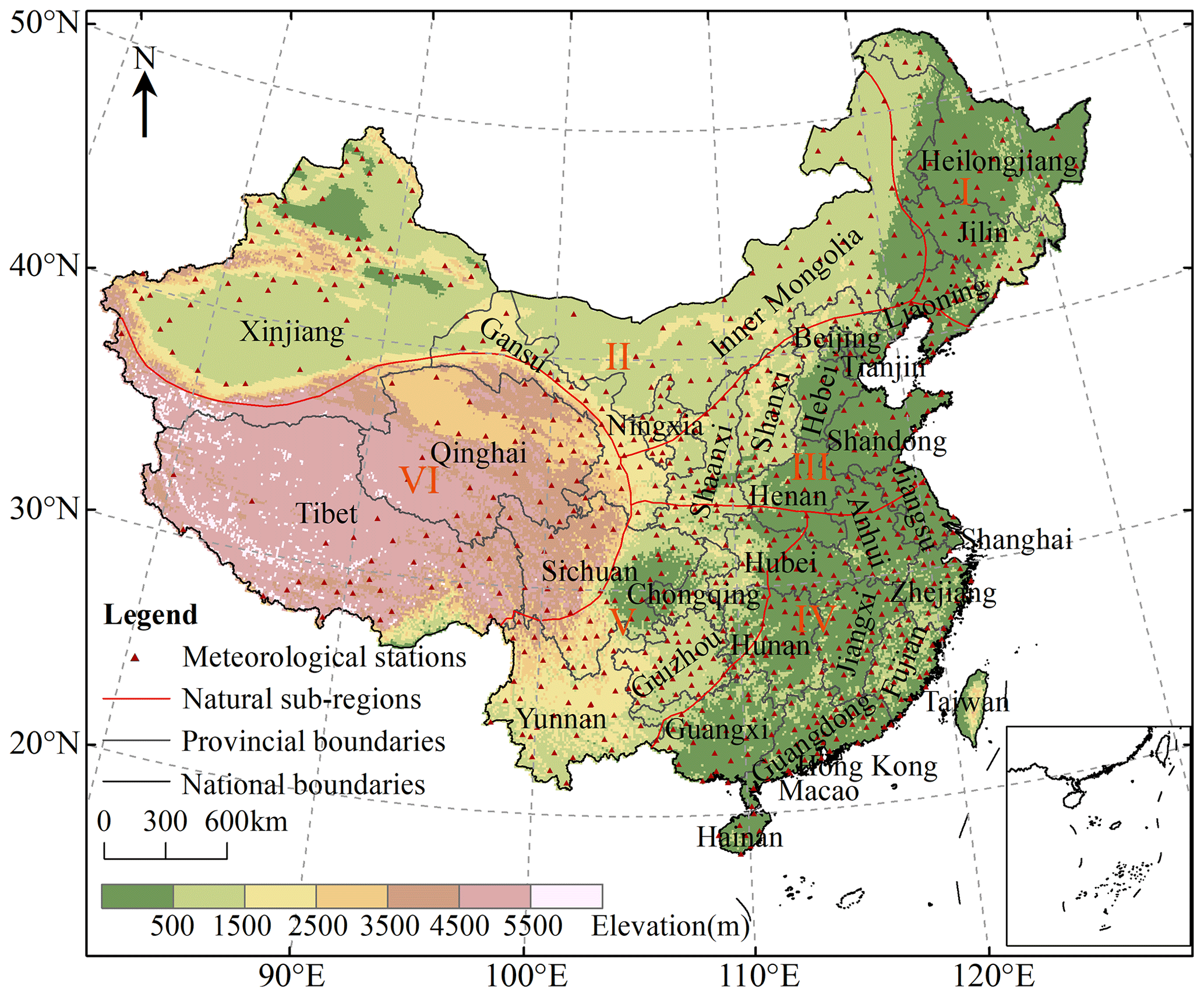
Figure 1Overview of the study area.
3.1 China Meteorological Forcing Dataset (CMFD)
CMFD is developed by the Hydro-meteorological Research Group of the Institute of Tibetan Plateau Research, Chinese Academy of Sciences. The dataset can be obtained from the National Qinghai–Tibet Plateau Science Data Center (https://data.tpdc.ac.cn/, last access: 9 December 2020). The near-surface Ta data of CMFD have a time resolution of 3 h and a spatial resolution of 0.1∘, and their accuracy in China is better than Global Land Data Assimilation System (GLDAS) data (He et al., 2020). CMFD data used ANUSPLIN software to interpolate the difference between GLDAS Ta data and the measured Ta data to obtain grid data, and then the difference grid data and the spatially downscaled GLDAS Ta data were spatially added to generate high resolution Ta data. The Ta data of CMFD have been widely used in climate simulation, hydrological simulation, vegetation greenness research and cross-validation of new Ta datasets (Luan et al., 2020; Gu et al., 2020; Wang et al., 2020). Although this dataset has become one of the most widely used climate datasets in China, it does not provide the Tmax value. In order to perform high temperature analysis, we need to construct a Tmax dataset.
3.2 ERA5 data
ERA5 data are the fifth generation of global climate reanalysis data produced by the European Centre for Medium-range Weather Forecast (ECMWF) after ERA-Interim. The model version used by ERA5 is IFS Cycle 41r2 and its spatial–temporal resolution and number of vertical layers are much higher than the ERA-Interim data (Hoffmann et al., 2019; Urraca et al., 2018; Hersbach et al., 2020). ERA5 reanalysis data provide a variety of meteorological elements including atmospheric parameters, land parameters and ocean parameters spanning a time range from 1950 to present. The data can be obtained from Copernicus Climate Data Store (https://cds.climate.copernicus.eu/, last access: 30 December 2020). The ERA5 dataset also does not provide the Tmax. This study used Ta data from 1979 to 2018 with a time resolution of 1 h and a spatial resolution of 0.25∘ to help build a Tmax estimation model to generate Tmax value, and we sampled the ERA5 data to the same spatial resolution as the CMFD data.
3.3 Meteorological station data
Tmax data from the China Surface Climatic Data Daily Dataset (V3.0) from 1979 to 2018 were used to verify the accuracy of Tmax estimations. The hourly Ta observation data from China meteorological stations were used to determine the occurrence times of Tmax and daily lowest air temperature (Tmin). Both datasets are from CMA National Meteorological Information Center (http://data.cma.cn/, last access: 9 December 2020). The data were subjected to preliminary quality control and evaluation by CMA, and all elements in the observational data are of high quality and completeness with the validity rate generally above 99 %. These datasets have been widely used in Chinese climate research (L. C. Li et al., 2019; Tong et al., 2019). To ensure the validity of the site data, manual checks were performed on all observed data including extreme value tests and spatial–temporal consistency tests, and continuous missing data due to instrument damage and other reasons were eliminated. There are 824 stations for Tmax observation data and 2633 stations for hourly Ta observation data. After performing checks and tests, we used Tmax data from 760 meteorological ground stations and hourly Ta data from 2421 meteorological ground stations.
3.4 Ocean climate modal indices
The ocean occupies about 71 % of the earth's surface area which has a great impact on climate change. After considering the distribution characteristics of China's land and sea, we analyzed the effects of the following ocean climate modal indices on high temperature in China: Indian Ocean basin warming (IOBW) index, North Atlantic Oscillation (NAO) index, and NINO3.4 area sea surface temperature (NINO3.4) index. Among them, the IOBW index comes from the National Climate Center of CMA (http://cmdp.ncc-cma.net/cn/index.htm, last access: 1 April 2021) and the NAO index and NINO3.4 index are from the National Oceanic and Atmospheric Administration of the United States (https://psl.noaa.gov/data/climateindices/list/, last access: 1 April 2021). The time range of the three indices is 1979–2018 and the time scale is monthly.
4.1 Tmax dataset construction
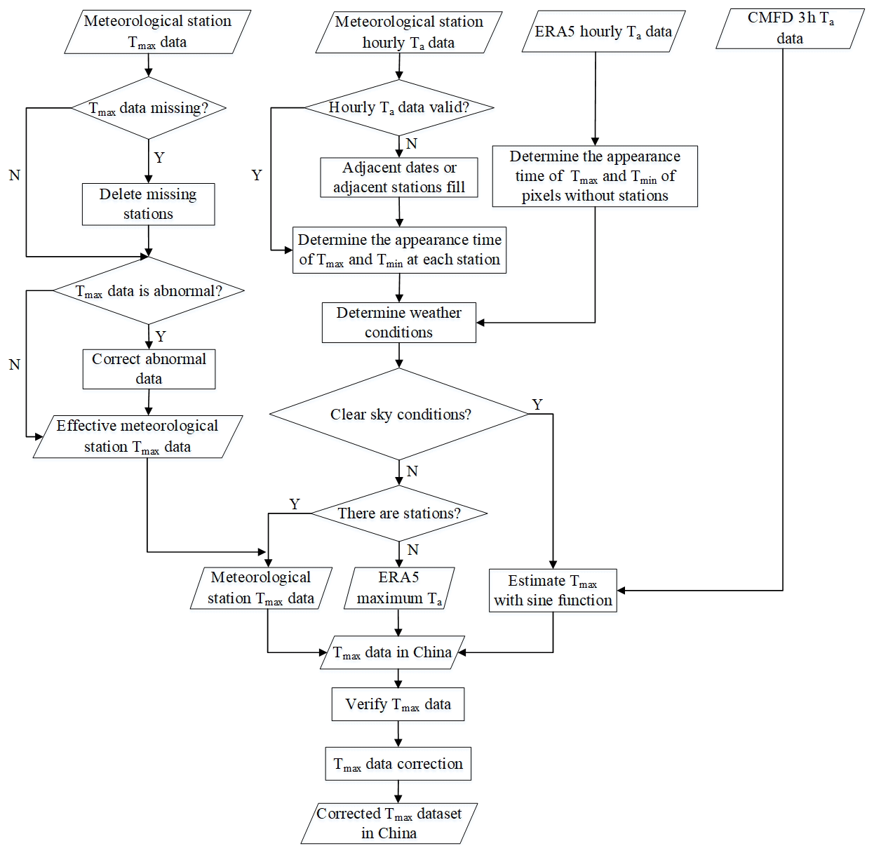
At present, the data used in the research on high temperature characteristics are mostly meteorological station data or grid data obtained by interpolation of station data. A limited number of stations cannot represent the high temperature distribution at large scale. For regions where the stations are very sparse, grid data obtained by spatial interpolation can hardly meet the accuracy requirements of high temperature feature analysis. Although LST can be used to estimate Tmax, LST has degraded value in the presence of clouds or rainfall. Therefore, in order to obtain a Tmax dataset with high temporal and spatial resolution, we propose a Tmax construction model that combines meteorological station data and reanalysis data, and consider the Tmax construction under clear sky and non-clear sky conditions (see Sect. 4.1.1 for details). The data processing process is shown in Fig. 2 and the data construction model is divided into two steps: Tmax estimation and Tmax correction. First, the occurrence time of Tmax and Tmin was determined pixel by pixel (see Sect. 4.1.1 for details). Then, Tmax was determined according to the weather state. (1) In clear sky conditions, CMFD 3h near-surface Ta data were used to construct the Ta diurnal variation model which, in turn, yielded Tmax. (2) In non-clear sky conditions, the site and reanalysis data were used to fill pixels. Finally, the correction model was used to correct the poor quality pixels to generate the final Tmax dataset in China.
4.1.1 Tmax estimation
The changes of Ta under different weather conditions are different. The changes of Ta under clear sky conditions are relatively smooth and regular. Under non-clear sky conditions, Ta changes more drastically. In order to improve the accuracy of Tmax estimation, we determined the occurrence time of Tmax and Tmin pixel by pixel. If there was a meteorological station at the pixel location, the analysis could be divided into two situations. (1) If hourly Ta data were valid, it was directly used to determine the occurrence time of Tmax and Tmin. (2) If there was a missing value in the hourly Ta data at a certain time, then we used the valid data from adjacent stations at the same time or adjacent time at the same stations to fill in the missing values. At present, there are not many meteorological stations in China and the pixels without stations account for 97.5 %. If there was no meteorological station at the pixel location, we used ERA5 hourly Ta data to determine the occurrence time of Tmax and Tmin. Since the spatial resolution of the ERA5 data is lower than that of the dataset we produce, in order to match the two data spatially, we sample the two data to the same resolution and then use latitude and longitude as control conditions to match the different data.
Studies have shown that the change of Ta under clear sky conditions follows a certain law: the change curve of Ta during the day is close to a sine function (Ephrath et al., 1996; Johnson and Fitzpatrick, 1977; Parton and Logan, 1981; Zhu et al., 2013) so we used sine function to simulate the change of Ta during the day. The appearance time of Tmin is tmin and the appearance time of Tmax is tmax. According to the periodicity of the sine function, the model of the change of Ta during the day is obtained like Eq. (1).
Here, n is the number of CMFD near-surface Ta data used to construct the Ta change model in a day. CMFD can obtain Ta data eight times a day. This study uses four daytime Ta data to construct a Ta variation model so n is 4. Tai is the near-surface Ta data at the ith time of CMFD and δ is the sum of squares of the difference between the model-estimated Ta and the near-surface Ta of the CMFD.
Since the change of Ta under non-clear-sky conditions does not conform to the sine curve change, we divided the estimation of Tmax under non-clear sky conditions into two situations. (1) If there was a station at the location of the pixel, the measured Tmax at the station was directly used as the Tmax of the pixel. (2) If there was no measured Tmax at the pixel location, the highest value of hourly Ta of ERA5 in a day was taken as Tmax. Then, Tmax determined by the ERA5 data was assigned to the pixel at the corresponding position of the Tmax image we established using the spatial matching method.
4.1.2 Tmax correction
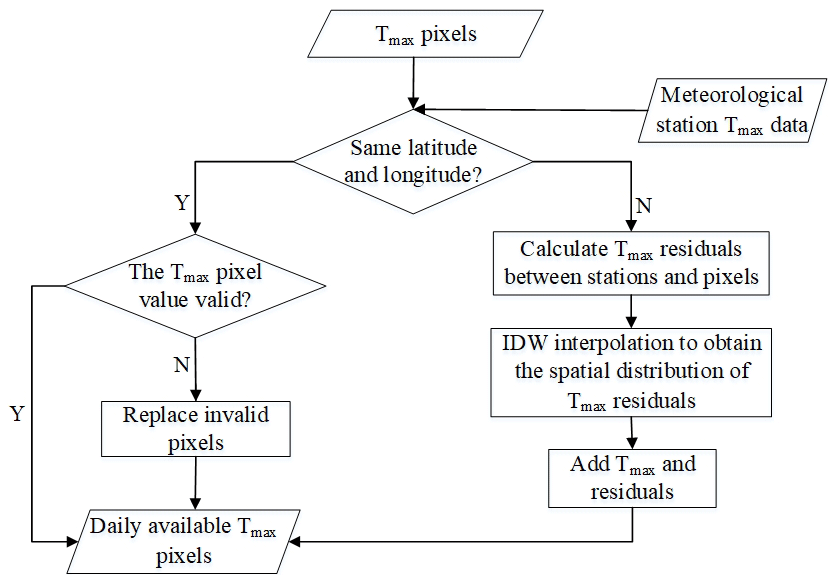
The validation of Tmax showed some differences between the estimated Tmax and the measured Tmax. In order to further improve the accuracy of Tmax, the measurements taken at weather stations should be used to correct the estimated Tmax as shown in Fig. 3. First, determine whether there are station data at the pixel location. For pixels with stations, if the difference between the estimated Tmax and the measured Tmax is less than 1 ∘C, we consider the Tmax of this pixel to be valid. For a pixel with poor quality, if there are station data at the location of the pixel, the low-quality pixel will be replaced with the measured data from the station. If there are no station data at the pixel location, the data are corrected by linear regression method (Ninyerola et al., 2000; Zhao et al., 2020; Zheng et al., 2013). By establishing the regression relationship on each day between station Tmax and estimated Tmax, the residuals were calculated according to the measured values and Tmax regression predicted values, and the spatial distribution of the residuals on each day was obtained by the inverse distance weight (IDW) interpolation method. Finally, the estimated Tmax and the residual were added to obtain the corrected Tmax. The calibration model is like Eqs. (3) and (4).
Here, i and j are the row and column numbers of the image, Tafter(i,j) is Tmax after correction, Tbefore(i,j) is Tmax before correction, is the residual, Ttrue(i,j) is the measured Tmax and Tforecast(i,j) is Tmax predicted by the regression model.
We used the jackknife method to randomly divide the station data into calibration and verification data (Benali et al., 2012; Zhao et al., 2020). We selected 80 % of the meteorological stations to establish the regression relationship between the measured and estimated Tmax values. The other 20 % of the meteorological stations were used to verify the accuracy of the corrected data. In order to improve data accuracy, the dataset used in the subsequent analysis of spatial–temporal variation of high temperature were the data corrected by all stations. Due to the different topographic and climatic characteristics of the six natural regions, the linear models of estimated Tmax and measured Tmax in each region were different. In order to obtain a higher-precision correction, the six regions were corrected separately.
4.2 Extreme temperature indices
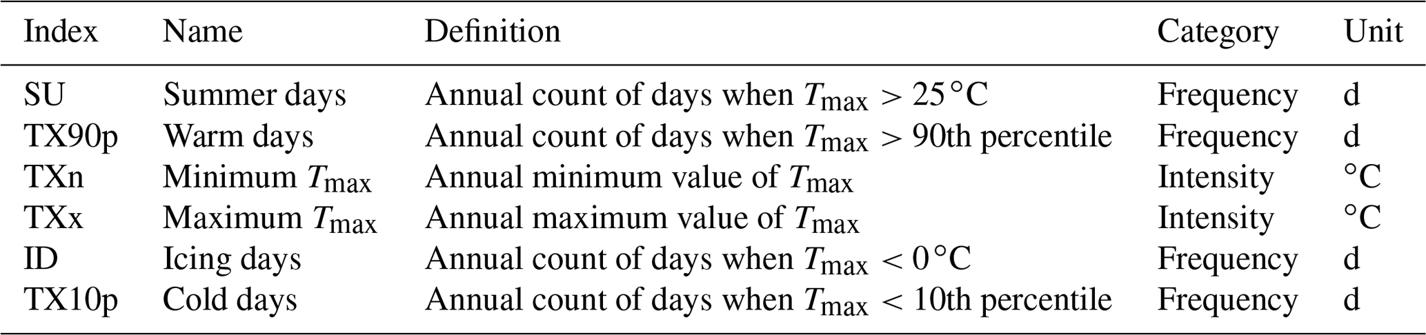
ETCCDI proposed a set of extreme climate indices in the Climate Change Monitoring conference which became the unified standard for climate change research (Hong and Ying, 2018; Mcgree et al., 2019; Poudel et al., 2020; Zhang et al., 2019; Zhou et al., 2016). Among them, 27 indices are considered as core indices which are calculated from daily Ta and precipitation data and have the characteristics of weak extremeness, low noise and strong significance. These indices comprehensively capture the frequency, intensity and duration of extreme climate events, and are recommended as the core indicators for extreme climate event analysis by the STARDEX program of the European Union (Guan et al., 2015; Ruml et al., 2017). In this study, six temperature indices related to Tmax were used to analyze high temperature characteristics, and their definitions are shown in Table 2. Among them, the 90th percentile in TX90p and the 10th percentile in TX10p were obtained in ascending order based on the Tmax data of each month during 1979–2018.
4.3 Trend analysis
4.3.1 Sen's slope estimation
In this study, the trends of Tmax and extreme temperature indices were calculated using Sen's slope estimation. Sen's slope estimation is a nonparametric estimation method. Even if there are some outliers in the sample, it can reliably estimate the change trend of the time series so it is widely used in trend analysis (Sen, 1968; Zhang et al., 2017). Eq. (5) is used to calculate the slope of each pair of data.
where , xk and xj are the time series values of the kth andjth samples, respectively (). Arranging the N, Ki values in ascending order, the median Sen's slope is estimated as Eq. (6).
4.3.2 Mann–Kendall trend test
Mann–Kendall trend test is used to test the trends of Tmax and extreme temperature indices. Mann–Kendall method does not require samples to follow a certain distribution and is not disturbed by a few outliers, and it can test the change trend of time series (Seenu and Jayakumar, 2021; Tan et al., 2019). Equation (7) is used to calculate the statistic of the Mann–Kendall trend test.
Here, xi and xj are the ith and jth data values of the time series, and n is the length of the time series where n is 40. Var(S) is the variance of S. The standardized statistic Zc is computed by using Eq. (10).
When , the change trend is considered to be significant. Here, is the standard normal variance, α is the significance test level when α=0.05, and when α=0.01, .
4.4 Mann–Kendall test for abrupt change analysis
Climate system change is an unstable and discontinuous change process, and one of the commonly used methods to test its change is the Mann–Kendall mutation test which is very effective in testing the change of elements from a relatively stable state to another state (Ruml et al., 2017). We used Mann–Kendall mutation test to test whether extreme temperature indices have mutation. For a time series x with n samples, Eq. (11) is used to construct an ordered sequence.
where sk is the cumulative count of the number of values at time i greater than that at time j. E(sk) and Var(sk) are the mean and variance of the cumulative number sk, respectively. UFk is a standard normal distribution given the significance level α and can be obtained from the normal distribution table. If |UFk|>Uα, this indicates that the variation trend of time series is significant. Reverse the time series x to and repeat the above process with .
4.5 Correlation analysis
Pearson correlation coefficient is often used to accurately measure the degree of correlation between two variables and its size can reflect the strength of the correlation of the variables. For variables and variables , the correlation coefficient between them is calculated as Eq. (16).
Here, n is the total length of the time series. The value of R is between −1 and 1. R<0 indicates a negative correlation. R>0 indicates a positive correlation. The closer the absolute value of R is to 1, the closer the relationship between the two elements is.
5.1 Validation
5.1.1 Validation of Tmax in each region
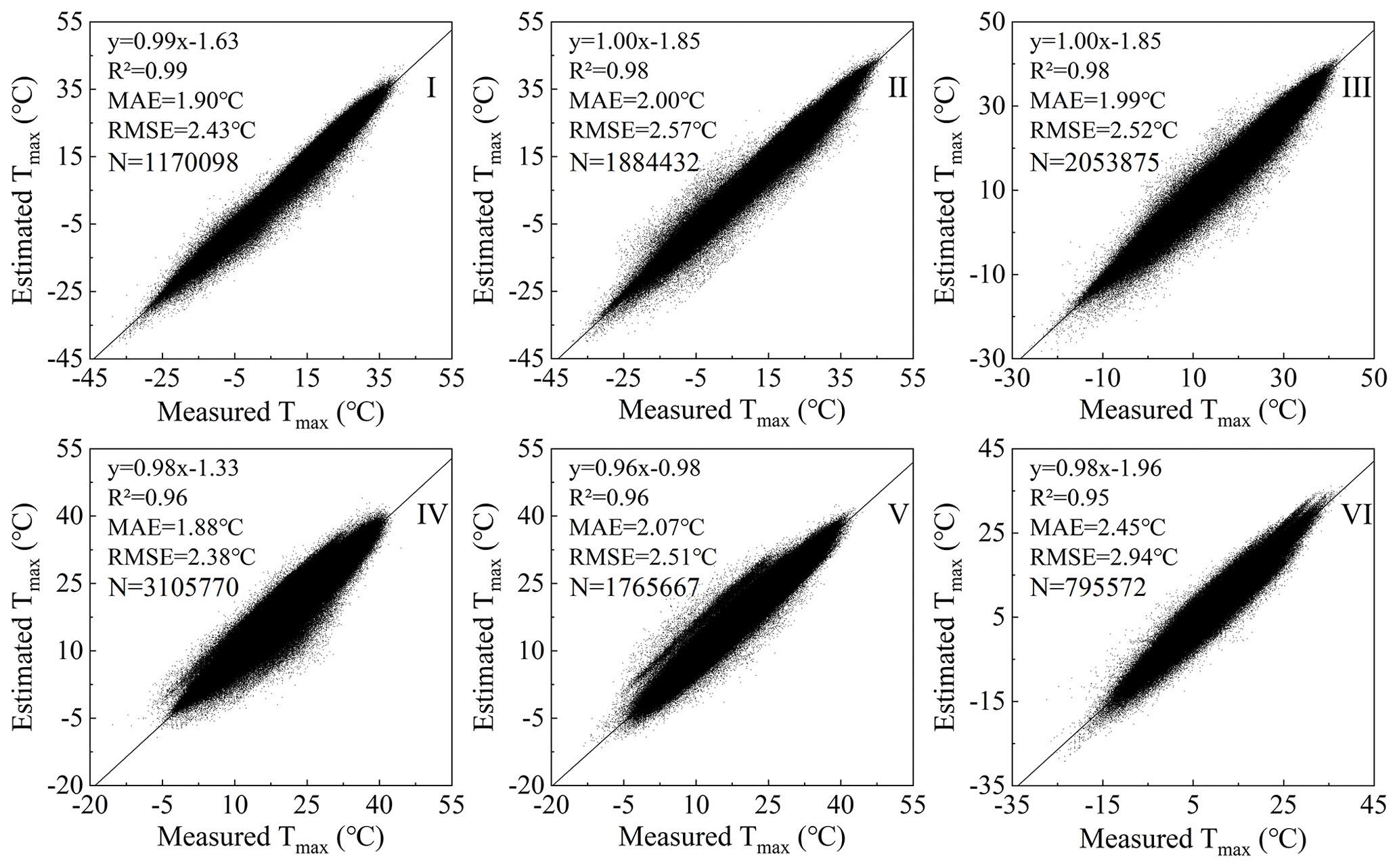
In order to verify the feasibility of Tmax estimation using the Ta diurnal variation model and to analyze the accuracy of Tmax estimation in different regions, scatter plots of estimated Tmax and measured Tmax in six natural regions (I, II, III, IV, V and VI) were drawn according to the regional division in Fig. 1. The results are shown in Fig. 4 and the validation in each region shows that the root mean square error (RMSE) is between 2.38 and 2.94 ∘C, the mean absolute error (MAE) is between 1.88 and 2.45 ∘C and the coefficient of determination (R2) is between 0.95 and 0.99. In six regions, the accuracy in region IV is the highest, while the accuracy is the lowest in region VI. As can be seen from Fig. 4, although most of the data are very accurate, some have some room for improvement. Therefore, further correction is needed to improve the accuracy of the Tmax dataset.
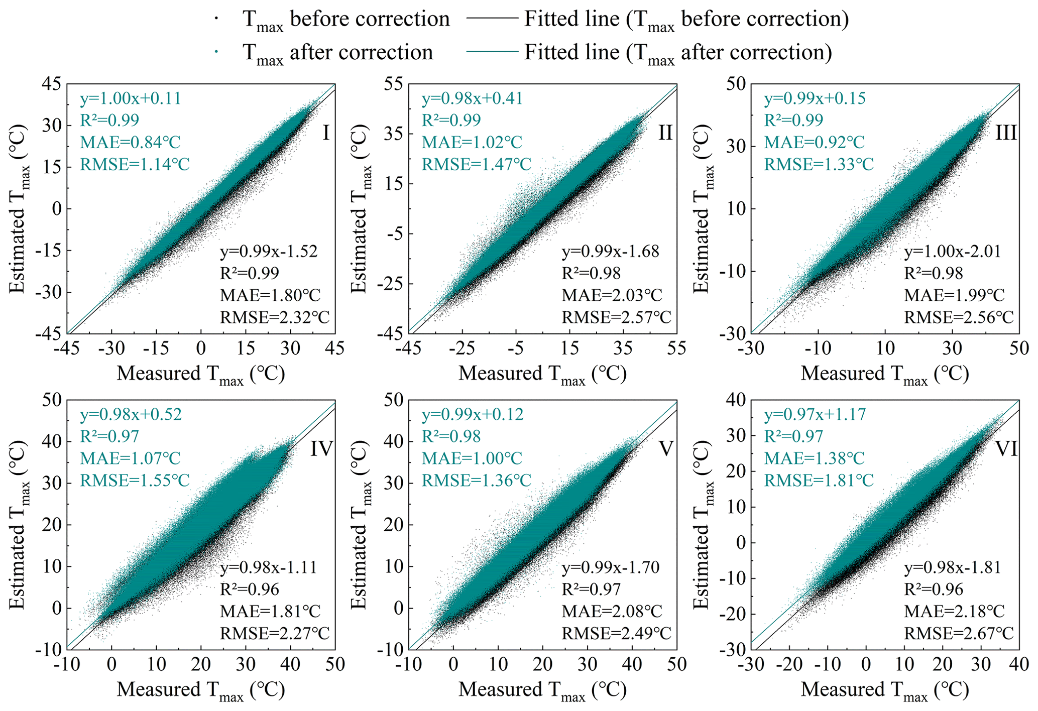
The correction method in Sect. 4.1.2 was used to correct the Tmax estimation results of six regions separately. The comparison between Tmax before and after correction with the measured Tmax is shown in Fig. 5. It can be seen that Tmax corrected by the regression model is more consistent with the measured Tmax. The RMSE decreases from 2.38–2.94 to 1.14–1.81 ∘C, the MAE decreases from 1.88–2.45 to 0.84–1.38 ∘C and the R2 increases from 0.96–0.99 to 0.97–0.99. The accuracy of Tmax is improved in each region after correction. The number of meteorological stations in region I is denser and the accuracy of Tmax after calibration is significantly improved. The RMSE reduced from 2.32 to 1.14 ∘C and the error is reduced by 51 %. The number of meteorological stations in region VI is small, and the topography is undulating and the spatial heterogeneity is large. Therefore, the accuracy in this region is still the lowest among the six natural areas after correction. In general, the corrected Tmax dataset has higher consistency with the measured data and can be applied to research related to regional-scale Tmax.
5.1.2 Validation of Tmax in the whole China region
Figure 6 shows the accuracy of Tmax before correction and Tmax after correction for the entire China region. It can be seen that the MAE of the corrected dataset is about 1.07 ∘C and the RMSE is 1.52 ∘C which is nearly 1 ∘C higher than that before correction. The accuracy evaluation result of the dataset for different years shows that the dataset in 2008 has the highest accuracy and the lowest in 2014 (Fig. 7). It can be seen from Fig. 8 that the dataset has the highest accuracy in September and the lowest accuracy in December. This may be because there is more clear sky weather in China in September and the daily temperature change curve is closer to a sine function which makes the Tmax estimation result more accurate.
In general, the Tmax dataset has a time range of 1979–2018, in Celsius with a temporal resolution of 1d and a spatial resolution of 0.1∘. It is produced by using meteorological station data and Ta reanalysis data (CMFD and ERA5) combined with diurnal variation model of Ta to establish Tmax data, and then a correction model is constructed to further correct the data to improve the data accuracy according to different geographic partitions. The accuracy assessments indicate that the dataset exhibits high accuracy and can be used for climate change analysis in China.
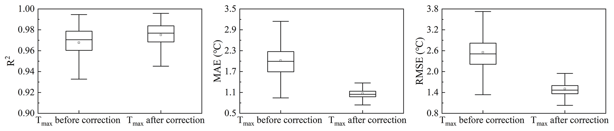
Figure 6Box plots of the R2, MAE and RMSE of comparison between Tmax before correction and Tmax after correction in the whole China region.
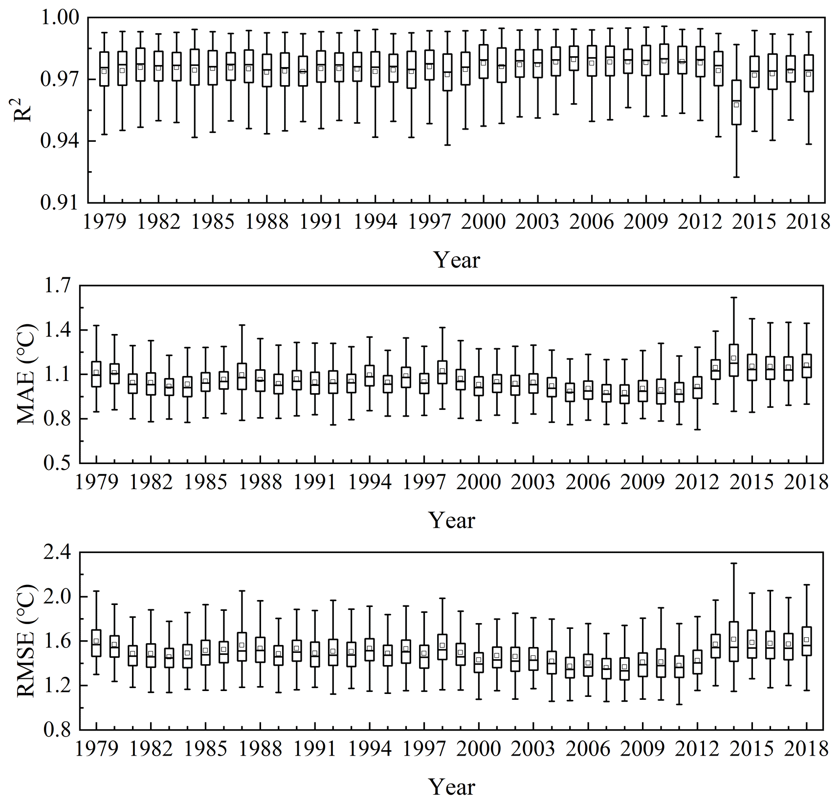
Figure 7Box plots of the R2, MAE and RMSE of Tmax after correction for each year in the whole China region.
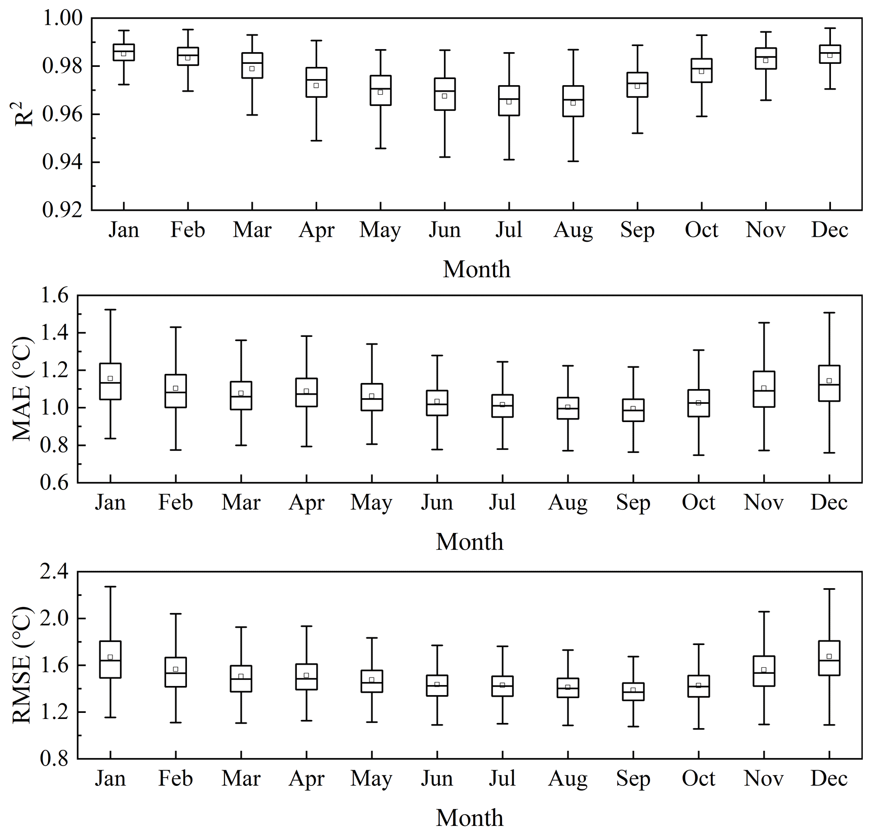
Figure 8Box plots of the R2, MAE and RMSE of Tmax after correction for each month in the whole China region.
5.2 Temporal and spatial changes of Tmax
5.2.1 Inter-annual variability
Figure 9 shows the annual average change of Tmax in each region of China during 1979–2018. The Tmax in each region exhibited an upward trend. However, due to the different geographical locations and the influence of atmospheric circulation in various regions, the change of Tmax was also different. The order of the Tmax increase in each region was V > IV > III > Whole > VI > II > I. The Tmax anomaly ranges of region I–VI and the whole China region were −1.41–1.53, −1.54–1.16, −1.47–1.12, −1.34–0.92, −0.97–1.33, −1.31–1.15 and −1.09–0.98 ∘C, respectively. The Tmax variation coefficients were 0.082, 0.045, 0.036, 0.024, 0.03, 0.088 and 0.038, respectively. It can be seen that Tmax fluctuated the most in region VI and the least in region IV. The minimum values of region I–VI and China region appeared in 1987, 1984, 1984, 1984, 1989, 1983 and 1984, respectively, which were distributed in the 1980s. The highest values of Tmax appeared in 2007, 2007, 2017, 2007, 2013, 1999 and 2007, respectively. Zhai et al. (2016) found that 1999, 2007 and 2013 were among the 10 years with the highest average Ta in China from 1900 to 2015. From 1998 to 2012, global surface temperature experienced a warming hiatus (Du et al., 2019; Li et al., 2015) and Tmax in all regions of China showed a downward trend during this period.

In order to understand the spatial pattern and regional differences of Tmax changes with more detail in China, Sen's slope estimation was used to calculate the annual average Tmax change rate from 1979 to 2018 at the pixel scale (Fig. 10a). The significance test of the Tmax change trend was conducted by the Mann–Kendall trend test (Fig. 10b). At the same time, the average change rate of Tmax in each region and the area percentage of significant increase and decrease (P<0.05) in Tmax were calculated (Table 3). The results indicated that the annual average Tmax change rate in most regions of China (78.24 % of the study area) passed the significance test with a significance level of 0.05, and 65.84 % of the pixels showed very significant changes in Tmax (P<0.01). Figure 10a showed that the annual average Tmax in most regions of China was on the rise and the fastest rising rate of Tmax was in western Yunnan. Only 8.13 % of the regions in China showed a downward trend in Tmax. These were concentrated mainly in the north and south of Xinjiang and the northwest and south of Tibet. Among the six regions, the average Tmax change rate of region V was the largest (0.38∘C per 10 years) and the average Tmax change rate of region I and region II was the lowest (0.31∘C per 10 years) (Table 3).
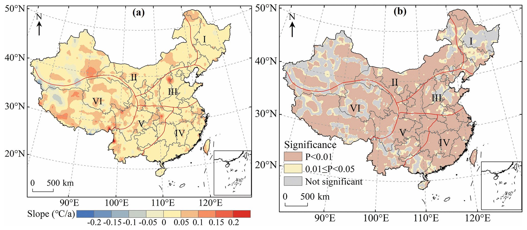
Figure 10Inter-annual change rate of Tmax (a) and results of Mann–Kendall trend test (b).
Table 3Statistics of Tmax change trends in various regions of China from 1979 to 2018.

5.2.2 Seasonal changes
On the basis of the annual analysis, we also analyzed the seasonal changes. The seasons are divided according to the months (spring from March to May, summer from June to August, autumn from September to November, and winter from December to February). We plotted the seasonal variation curve of Tmax in China from 1979 to 2018 (Fig. 11) and some information on the trend of Tmax changes is shown in Table 4. The results indicated that Tmax in each region fluctuated the most in winter and the least in summer. The highest Tmax in each region in spring, summer, autumn and winter mostly occurred in 2018, 2013, 1998 and 2007, while the minimum Tmax in each region in spring, summer, autumn and winter mostly occurred in 1988, 1993, 1981 and 1984. In 2013, Tmax of region IV-VI in summer reached the highest since 1979 mainly due to the influence of the southwest monsoon, East Asian summer monsoon and other factors. Under the influence of El Niño, Tmax in winter in region I, II and the whole study area was the highest in 2007. Under the influence of La Niña, the minimum Tmax in spring and winter in most areas of China appeared in 1988 and 1984, respectively. In the same season, the variation trend of Tmax in each region was significantly different and some even had opposite trends. However, influenced by La Niña and the Eurasian atmospheric circulation, Tmax in winter in each region showed a consistent decreasing trend from 2007 to 2008. As can be seen from Table 4, in spring, summer, autumn and winter, the regions with the fastest Tmax rise are III, I, I and VI respectively, and the regions with the lowest Tmax change rate are VI, VI, III and II, respectively.
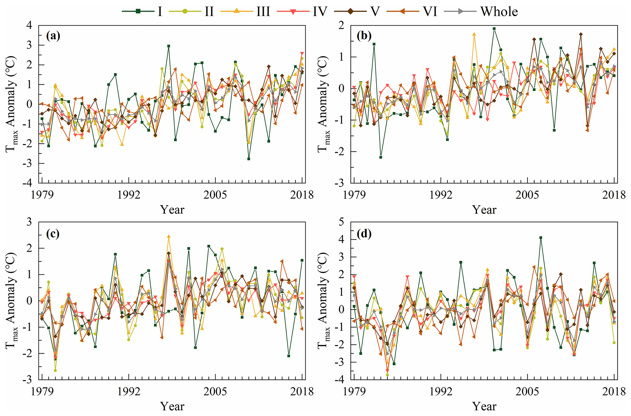
Figure 11Changes of Tmax anomalies in various regions of China in spring (a), summer (b), autumn (c) and winter (d) during 1979–2018.
Table 4Seasonal change rate of Tmax in various regions of China from 1979 to 2018.
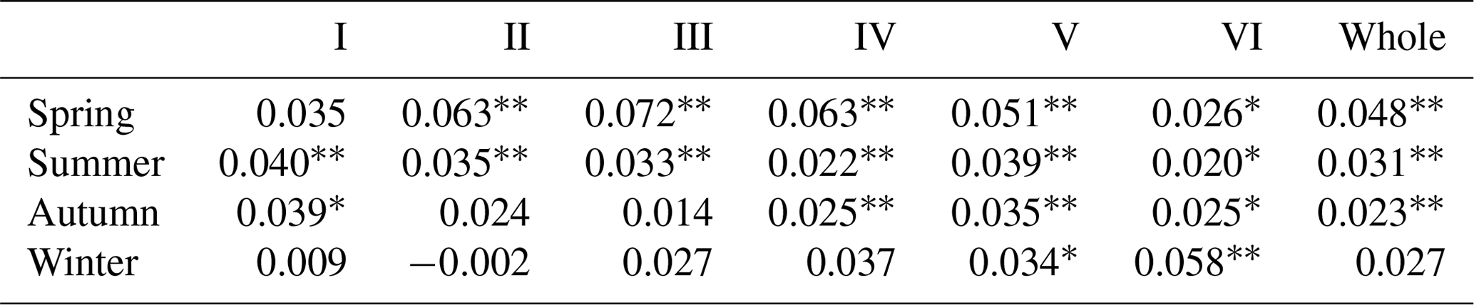
*, represent the trends that are significant at the level of p=0.05, p=0.01, respectively.
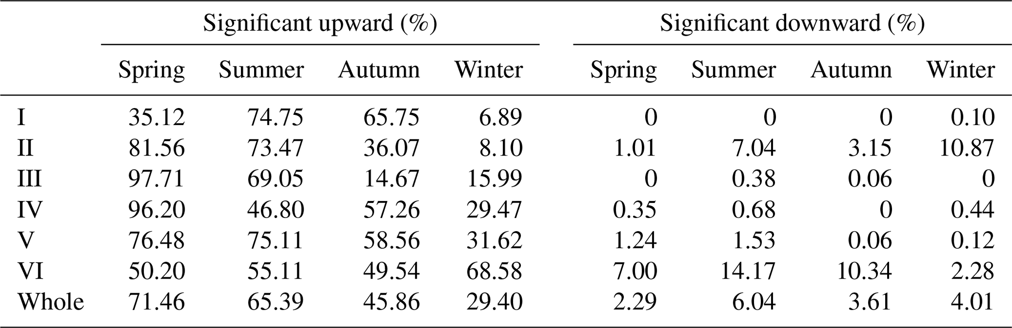
In order to display the seasonal variation characteristics of Tmax in China more intuitively, we drew the spatial distribution of the trend of Tmax and conducted a significance test (Fig. 12). Meanwhile, we counted the percentage of significant increase and decrease in Tmax in each region (Table 5). The results indicated that the areas with increasing Tmax were more than those with decreasing Tmax in all seasons. From 1979 to 2018, the increasing trend of Tmax was most significant in spring which accounted for 92.73 % of the total study area followed by autumn and summer, while Tmax increased the least in winter. Specifically, Tmax increased significantly in most parts of China in spring and the region where Tmax decreased significantly was mainly concentrated in the region VI (Fig. 12a). In summer, Tmax in most part of China showed a significant increasing trend, but Tmax in southern Xinjiang and northwestern Tibet exhibited a decreasing trend (Fig. 12b). Compared with spring and summer, the area with a significant increasing trend of Tmax in autumn was smaller and the regions with a significant decreasing trend of Tmax were mainly distributed in Xinjiang and Tibet (Fig. 12c). In winter, 79.02 % of the regions experienced an increase in Tmax which was significantly lower than in other seasons. A significant increasing trend of Tmax was observed in the east of region IV and the southwest of regions V and VI while the areas where Tmax decreased significantly were mainly observed in Xinjiang (Fig. 12d). We also observed no significant decrease in Tmax in regions I and III in spring, I in summer, I and IV in autumn, and III in winter (Table 5). Further statistics showed that Tmax of the whole region III showed an upward trend in spring.
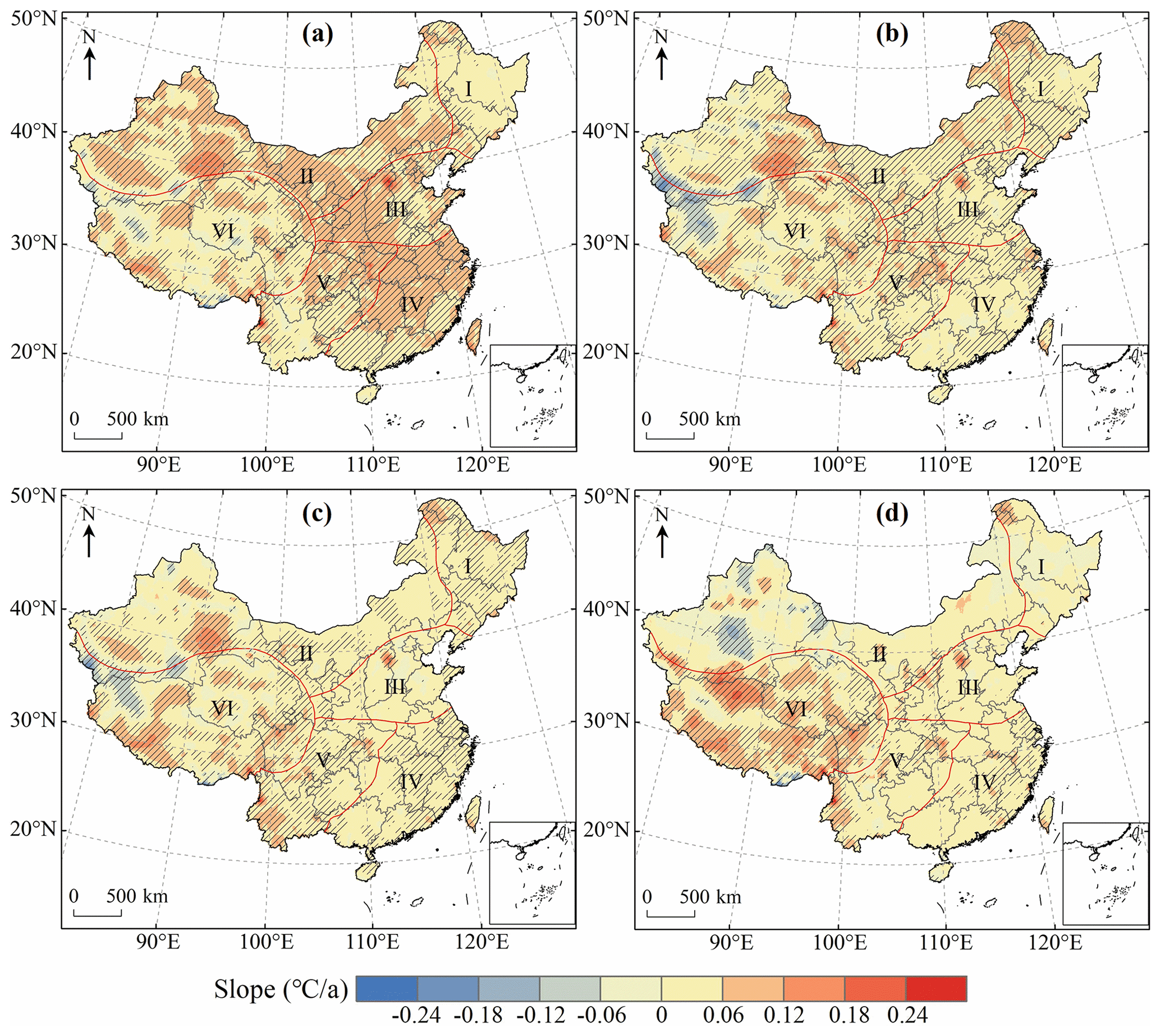
Figure 12Spatial distribution of the change trend of Tmax in spring (a), summer (b), autumn (c) and winter (d) over China during 1979–2018. The shaded areas indicate trends that are significant at the 0.05 level.
Table 5Change trend statistics of Tmax in different seasons over China from 1979 to 2018.
5.3 Temporal and spatial changes of extreme temperature indices
5.3.1 Change of time
We plotted the inter-annual variation of extreme temperature indices anomalies in various regions of China from 1979 to 2018 (Fig. 13), and used Sen's slope estimation and the Mann–Kendall trend test to calculate statistics on the trend of extreme temperature indices (Fig. 14). The results indicated that SU, TX90p, TXn and TXx increased at a rate of 3.83d/10a, 6.57d/10a, 0.11∘C per 10 years and 0.32∘C per 10 years, respectively (Fig. 14). Influenced by the strong El Niño in 1997, the SU in all regions exhibited a consistent upward trend from 1996 to 1997 (Fig. 13). The change rate of SU in all regions passed the significance test of 0.01 indicating a significant upward trend (Fig. 14). The increasing trend of TX90p in all regions was also very significant. The decadal average of TX90p in regions III–VI and the whole study area had an increasing trend, while the decadal average of TX90p in region I and region II increased first and then decreased slightly. The TXn of region II showed a weak decreasing trend and the sliding average of the 3-year and 5-year periods also exhibited a weak fluctuation downward trend. TXn of other regions showed an upward trend in general and only region VI had a significant increasing trend (P<0.05) (Fig. 14). Except for region VI, the change rate of TXx in other regions was higher than that of TXn. The rate of change of TXx exhibited that the upward trend of region VI was not significant, while all other regions passed the significance test of 0.01. During 1979–2018, ID and TX10p decreased significantly at the rate of −1.48d/10a and −3.78d/10a, respectively (P<0.01) (Fig. 14). The ID of all regions exhibited a downward trend with region VI and the whole study area showing the most obvious decline passing the significance test of 0.01 (Fig. 14). Compared with ID, TX10p decreased more sharply and the highest value of TX10p in all regions occurred before 1988 (Fig. 13). The above results indicate that the frequency of high temperature events in China is on the rise which is in line with the expected results of global change. In addition, we also found that the occurrence time of maximum and minimum values of SU, TXn, TXx and ID during 1979–2018 was consistent with previous research results by Hong and Ying (2018) which further proved the correctness of the Tmax dataset constructed by us, indicating that the dataset can be used to analyze the spatial–temporal changes of high temperature in China.
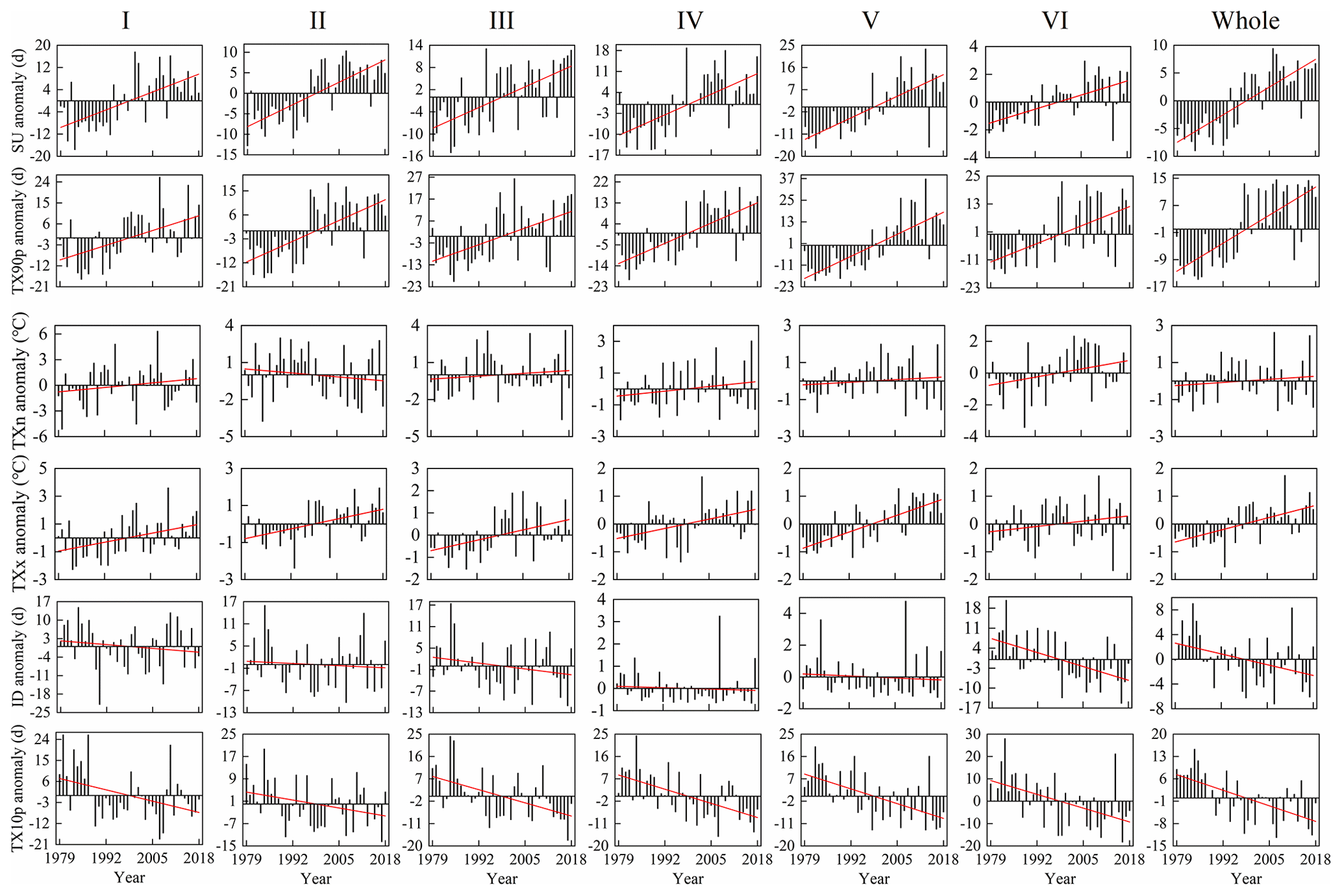
Figure 13Inter-annual trend of extreme temperature indices anomalies in different regions of China during 1979–2018.
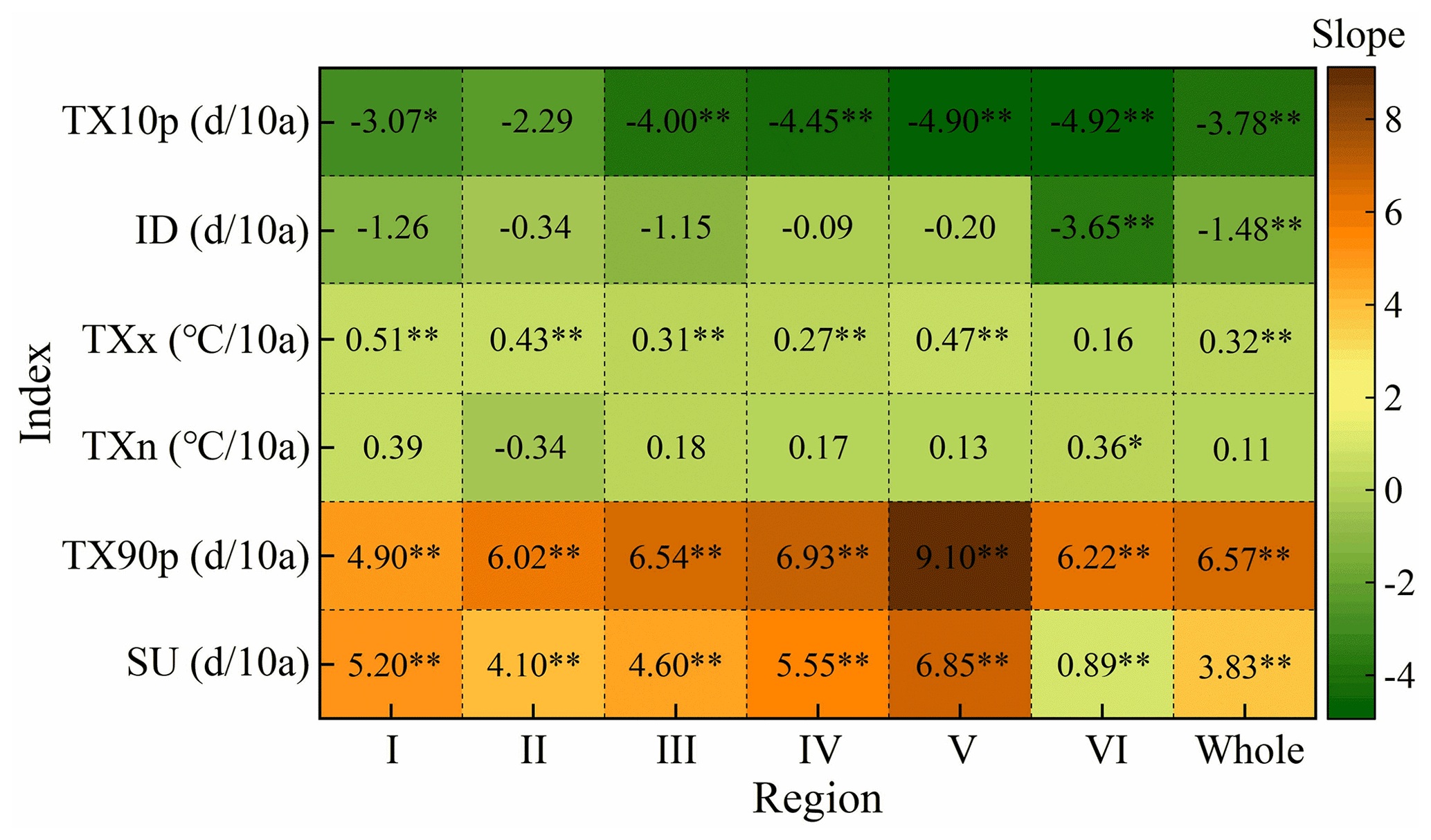
Figure 14Variation trend of extreme temperature indices in different regions of China from 1979 to 2018. (* significant at the 0.05 level, significant at the 0.01 level.)
In order to analyze the variation rules of extreme temperature indices in China from 1979 to 2018, the Mann–Kendall mutation test was applied to test the mutation characteristics of six extreme temperature indices at the significance level of 0.05. The results are shown in Fig. 15. We found that all the extreme temperature indices had abrupt change from 1979 to 2018 and 40 % of the years where the abrupt changes occurred were El Niño years while 46.7 % were La Niña years. This finding further confirms that China is greatly affected by global climate change. TX90p in region I–II and the whole study area displayed an abrupt change from a period with lower value to one with higher value in 1996. After mutation in region II in 2003, TXn turned from an upward trend to a downward trend but the downward trend was not obvious. The ID of the whole study area and its six sub-regions tended to increase first and then decrease.
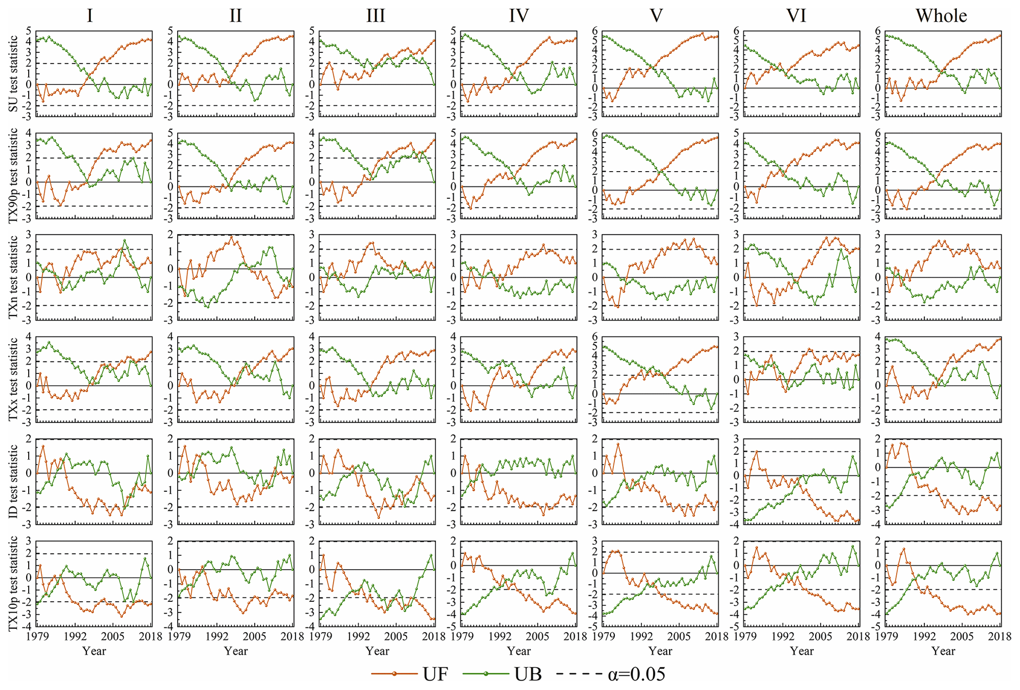
Figure 15MK abrupt change detection for the extreme temperature indices in different regions of China during 1979–2018.
5.3.2 Spatial change
The spatial distribution of the extreme temperature indices trends in China during 1979–2018 is shown in Fig. 16a–f while the area percentage of the increasing and decreasing trend of extreme temperature indices in each region is shown in Fig. 17a–f. For SU, TX90p, TXn and TXx, the area with rising trend is larger than the area with declining trend. The change of SU in most regions of China passed the significance test of 0.05 and the areas with significant increase accounted for 63.3 % of the whole study area (Fig. 17a). The regions with no significant change in SU were mainly distributed in region VI (Fig. 16a). There were few days in a year when Tmax exceeded 25 ∘C in region VI and Tmax in some regions was even lower than 25 ∘C throughout the year so the change range of SU was small. The areas with a downward trend of TX90p were mainly distributed in southern Xinjiang and northern Tibet (Fig. 16b). TX90p increased significantly in 75 % of regions in China (P<0.05) and the area percentage of TX90p that significantly increased in region V was the largest among the six regions (Fig. 17b). The trend of TXn change in most regions of China was not significant and the significant decrease was mainly concentrated in region II and region VI (Fig. 16c). While other regions were dominated by increasing trend of the TXn, 69.7 % of regions in region II showed a downward trend (Fig. 17c). For TXx, its upward trend was slightly stronger than TXn and the region with the highest change rate was located in western China (Fig. 16d). The regions with significantly decreased ID were mainly distributed in region VI (Fig. 16e). There was a declining ID in 75.7 % of the regions and 53 % of the regions passed the significance test (Fig. 17e). As far as TX10p is concerned, its cooling trend was much stronger than that of ID and the areas of significant decline were widely distributed through all regions of China (Fig. 16f). The area with a significant decrease in region IV accounted for 75.9 % of the region which was the largest among the six regions (Fig. 17f).
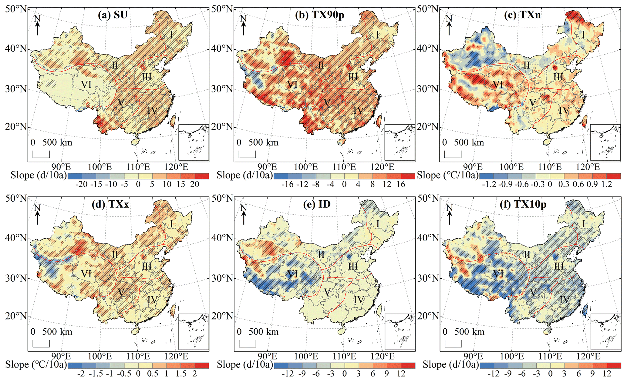
Figure 16Spatial distribution of trends in extreme temperature indices over China during 1979–2018. The shaded areas indicate trends that are significant at the 0.05 level.

Figure 17Area percentage of the trend of extreme temperature indices in different regions of China during 1979–2018.
6.1 The influence of ocean climate modalities on Tmax
The correlation between Tmax anomalies and three climate modal indices in China during 1979–2018 is shown in Fig. 18a–c. The results show that there is a significant positive correlation between Tmax and IOBW in 54.18 % of the regions in China which indicates that the warming of the Indian Ocean will contribute to the warming trend of Tmax in these regions. Tmax had a moderate positive correlation (, P<0.01) with IOBW in southern Yunnan and eastern Hainan (Fig. 18a). Tmax and NAO had a significant positive correlation in northeast China but the correlation was very weak (R<0.2). The percentage of Tmax anomaly value negatively correlated with NAO (16.55 %) was higher than that of NAO positively correlated (5.27 %) mainly distributed in the west and south of region II, west of region III, south of region IV and V, and northeast of region VI. This indicated that the positive phase of NAO contributes to the decrease in Tmax in these regions (Fig. 18b). Tmax was significantly positively correlated with NINO3.4 in southern China, central Xinjiang and southern Gansu indicating that El Niño events will lead to higher temperatures in these regions. In western China and the middle part of region IV, Tmax was significantly negatively correlated with NINO3.4 indicating that El Niño events will lead to cooling phenomena in these regions (Fig. 18c).
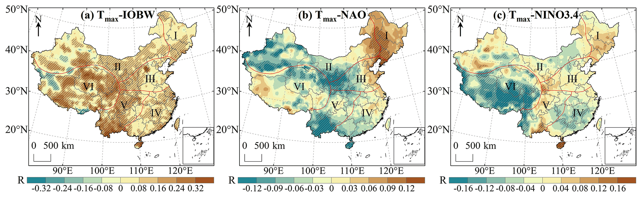
Figure 18Correlation analysis between Tmax and IOBW (a), and NAO (b) and NINO3.4 (c) in China during 1979–2018. The shaded areas indicate correlations that are significant at the 0.05 level.
6.2 The influence of ocean climate mode on extreme temperature indices
Figure 19a–f indicates the spatial distribution of the correlation between extreme temperature indices anomalies and IOBW in China during 1979–2018. It can be seen that SU, TX90p, TXn and TXx over most of China are positively correlated with the IOBW. The region with significant positive correlation between the SU and IOBW accounted for 42.67 % of the whole study area which indicated that a warming Indian Ocean would lead to the number of days over 25 ∘C in these regions to increase. Significant negative correlations were found in northwest and southeast Tibet and the mountainous regions of southern Xinjiang (Fig. 19a). The area with the largest correlation coefficient is in the northeast of Hainan (R=0.48). The significant negative correlation between TX90p and IOBW was mainly distributed in region VI but the negative correlation was not strong () (Fig. 19b). The correlation coefficient between TXn and IOBW ranged from −0.34 to 0.34 and the regions with significant positive correlation accounted for 16.65 % of the whole study area. TXn and IOBW were significantly negatively correlated mainly in western China (Fig. 19c). Compared with TXn, the regions with significant correlation between TXx and IOBW were more widely distributed in China among which the correlation coefficients in southern Yunnan and eastern Hainan were moderately positive () (Fig. 19d). ID and TX10p were negatively correlated with IOBW in most of China. The regions with significant negative correlation between ID and IOBW were mainly distributed in region VI and the regions with significant positive correlation were mainly distributed in the west of region II (Fig. 19e). TX10p has a significant negative correlation with IOBW in more areas than ID and the significant positive correlation was mainly located in western China (Fig. 19f).
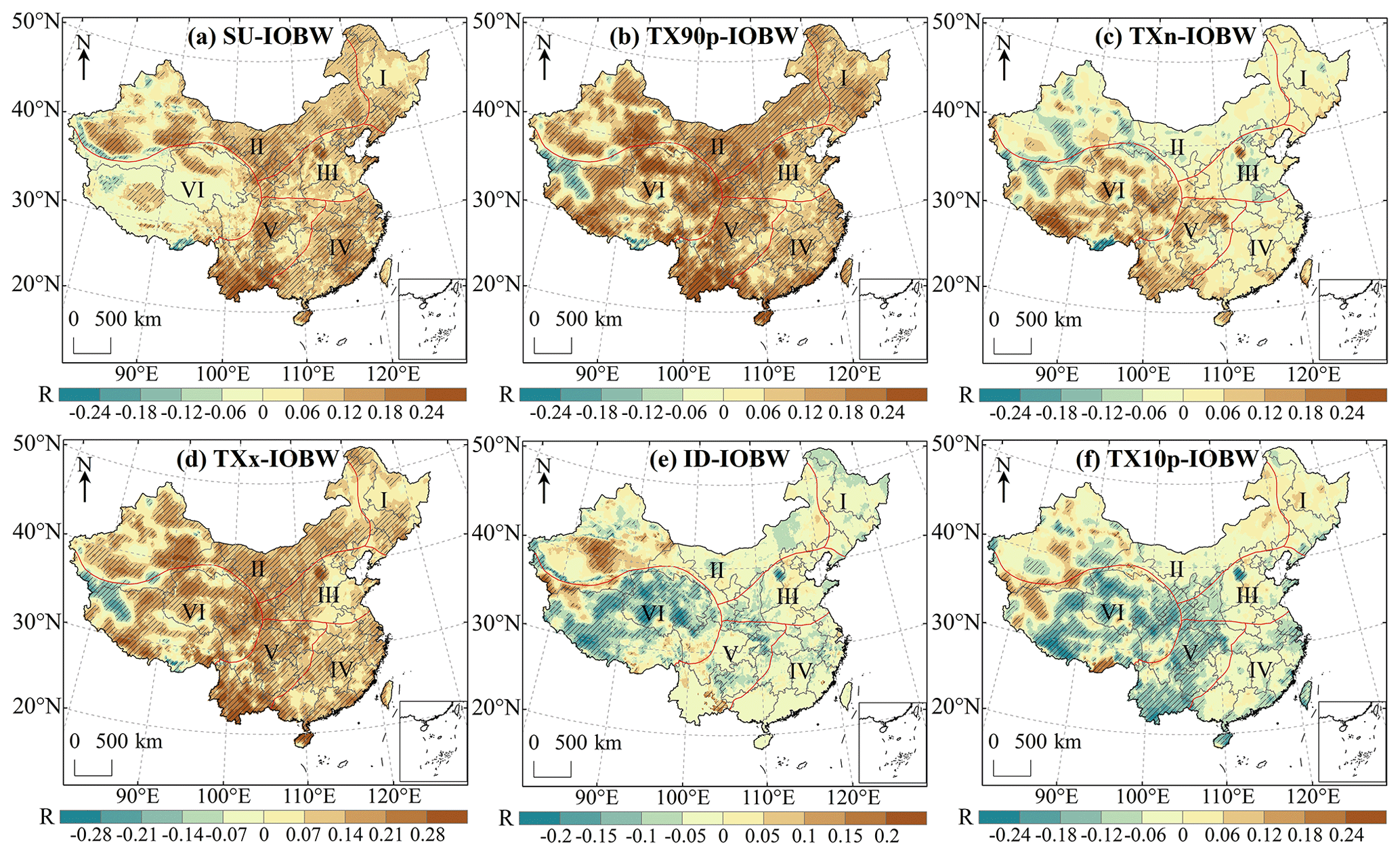
Figure 19Correlation analysis between extreme temperature indices and IOBW in China during 1979–2018. The shaded areas indicate correlations that are significant at the 0.05 level.
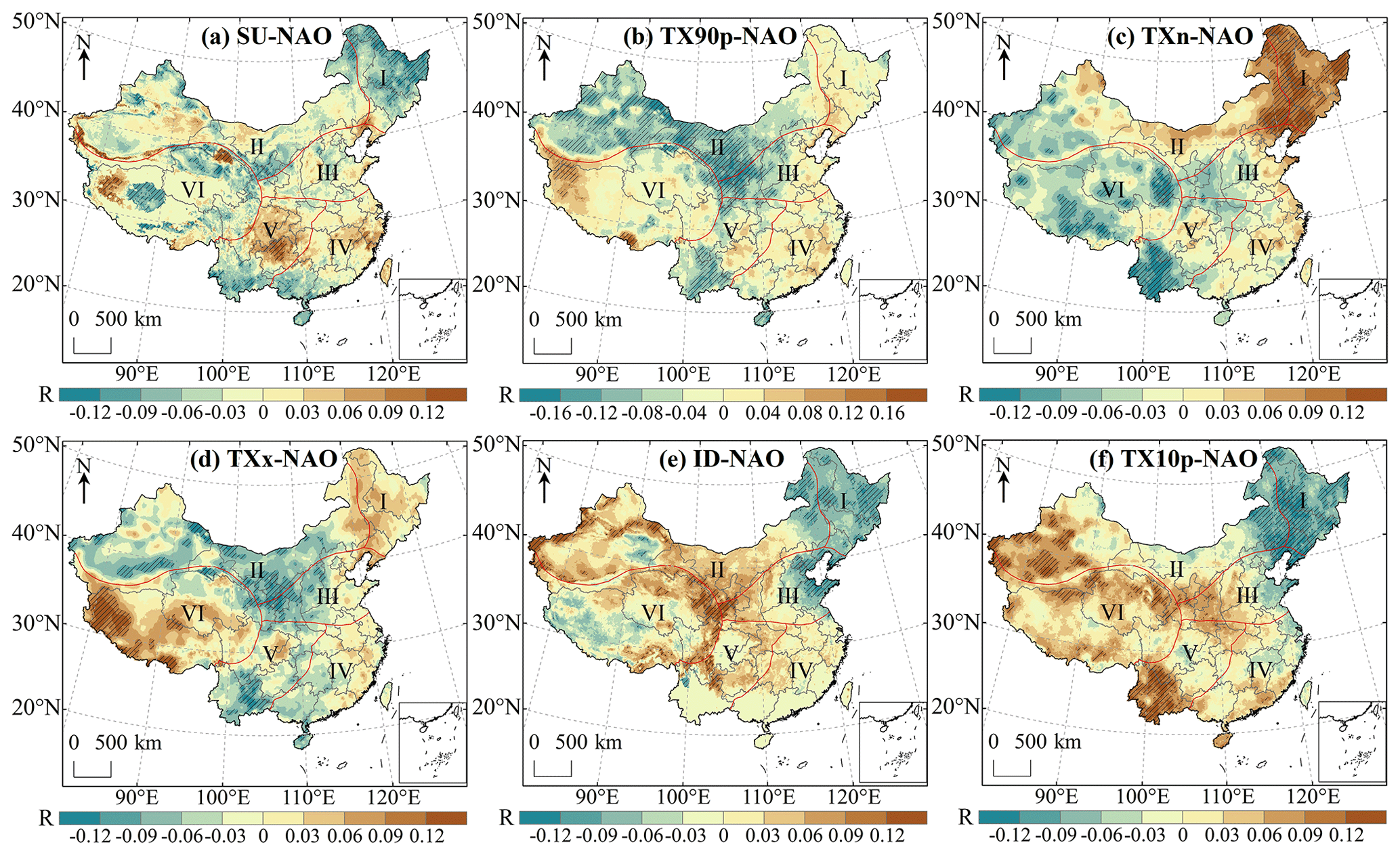
Figure 20Correlation analysis between extreme temperature indices and NAO in China during 1979–2018. The shaded areas indicate correlations that are significant at the 0.05 level.
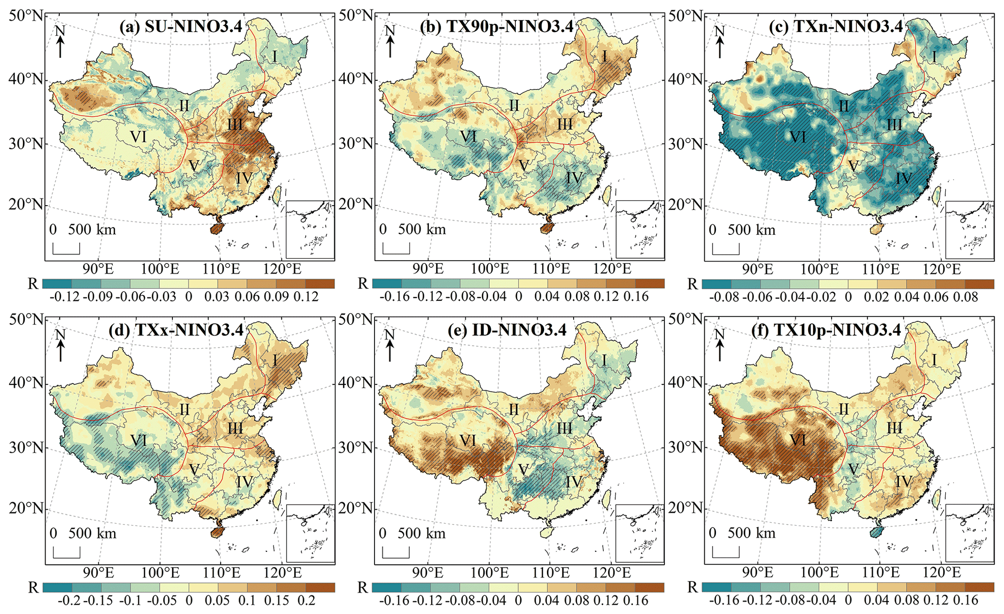
Figure 21Correlation analysis between extreme temperature indices and NINO3.4 in China during 1979–2018. The shaded areas indicate correlations that are significant at the 0.05 level.
The influence of NAO on the extreme temperature indices is shown in Fig. 20a–f. SU, TX90p, TXx and TXn were negatively correlated with the NAO more than they were positively correlated with NAO indicating that the positive phase of NAO would lead to the decline of SU, TX90p, TXx and TXn over most of China. SU and NAO had a significant positive correlation in southern Xinjiang, western Tibet, northern Qinghai and northern Guizhou but the correlation was very weak (R<0.2). There was no significant correlation between SU and NAO in southern Qinghai, which was consistent with previous observations (Ding et al., 2018). The region with the strongest negative correlation between SU and NAO was located in Tibet (8) (Fig. 20a). TX90p had a weak negative correlation with NAO in eastern Xinjiang (, P<0.01). TX90p was significantly positively correlated with NAO in the west and south of region VI but the correlation was extremely weak (Fig. 20b). Shi et al. (2019) indicated that more regions had a significant positive correlation between TXn and NAO in China than a significant negative correlation which was consistent with our results. The areas of TXn that had a significant positive correlation with NAO were mainly distributed in northeast China while the regions with significant negative correlation were mainly located in central Tibet, eastern Qinghai and Yunnan (Fig. 20c). The correlation coefficient between TXx and NAO varied from −0.16 to 0.21. The regions with significant positive correlation between TXx and NAO were mainly located in Tibet and the region with the strongest correlation was located in southern Tibet (Fig. 20d). The areas of ID that were significantly positively correlated with NAO accounted for 5.86 % of the whole study area and the strongest correlation was found in western Xinjiang (R=0.23). The regions with significant negative correlation between ID and NAO were mainly distributed in eastern and northeastern China (Fig. 20e). Sun et al. (2016) found a very weak positive correlation between TX10p and NAO in the Loess Plateau which was consistent with our results. The regions with a significant negative correlation were mainly concentrated in northeastern China (Fig. 20f).
Figure 21a–f shows the correlation between NINO3.4 and extreme temperature indices. The regions with significant positive correlation between SU and NINO3.4 were mainly distributed in eastern China indicating that the events of El Niño would lead to an upward trend of SU in these regions. There were few regions with significant negative correlation between SU and NINO3.4, only accounting for 1.15 % of the entire research area, mainly distributed in southeast Tibet and southwest Yunnan (Fig. 21a). The correlation coefficient between TX90p and NINO3.4 was −0.19–0.26. The areas of TX90p that had a significant negative correlation with NINO3.4 were mainly distributed in region IV and VI (Fig. 21b). There was a significant negative correlation between TXn and NINO3.4 in 24.59 % of regions and the region with the strongest negative correlation was located in Tibet (). TXn was positively correlated with NINO3.4 in only 10.46 % of regions in China and the region with the largest correlation coefficient was northwest Xinjiang (R=0.11) (Fig. 21c). There was a weak positive correlation between TXx and NINO3.4 in southern Guangdong and northern Hainan (). The regions of TXx significantly negatively correlated with NINO3.4 were mainly distributed in the south of region V and region VI (Fig. 21d). The significant negative correlation between ID and NINO3.4 was mainly concentrated in southern China. The areas with significant positive correlation were mainly distributed in the western region II and southern region VI, and the region with the strongest correlation was located in the western Sichuan (R=0.31) (Fig. 21e). TX10p in most regions of regional VI was significantly affected by NINO3.4 and the significant positive correlation area accounted for 69.31 % of the whole region VI. TX10p was significantly negatively correlated with NINO3.4 in only 0.65 % of regions in China mainly distributed in Hainan and southern Gansu (Fig. 21f).
The global temperature continues to rise and extreme weather events continue to increase (IPCC, 2021). It is of great significance to study regional high temperature changes. In order to obtain the key parameters of high temperature spatial–temporal variation analysis, this study proposed a daily Tmax estimation frame based on the near-surface Ta grid data and Ta diurnal variation model to build a Tmax dataset in China from 1979 to 2018. Validation of Tmax estimation data in six natural regions indicated that the RMSE of each region was between 2.38 and 2.94 ∘C, the MAE was between 1.88 and 2.45 ∘C and R2 was between 0.95 and 0.99. After using the regression model to calibrate the dataset, the accuracy of the estimated Tmax has been significantly improved. The RMSE of the Tmax after calibration reduced to 1.14–1.81 ∘C, the MAE reduced to 0.84–1.38 ∘C and the R2 increased to 0.97–0.99.
This dataset was used to study the spatial–temporal variation characteristics of Tmax and the corresponding influencing factors in China, and to discuss the correlation between Tmax, extreme temperature indices and ocean climate modal indices. Tmax in all regions of China exhibited an upward trend from 1979 to 2018 with the largest rise in region V and the smallest rise in region I. In spring, Tmax in China increased significantly in most regions and region III has the fastest rising speed. In winter, Tmax in China had the least significant rise and region II had the slowest rise rate. SU, TX90p and TXx in all regions showed an upward trend. Except for region II, TXn in other regions also exhibited an upward trend while ID and TX10p in all regions showed a downward trend. All extreme temperature indices had abrupt changes during 1979–2018, and most of the abrupt changes occurred in El Niño or La Niña years. The region with the largest increase in SU, TX90p and TXx and the region with the largest decrease in TX10p were located in western Yunnan. The correlation analysis between Tmax and extreme temperature indices and ocean climate modal indices indicated that the increase in the IOBW usually coincides with the increase in Tmax, SU, TX90p, TXn and TXx and the decrease in ID and TX10p. NAO had the opposite relationships. In most regions of China, Tmax, SU, TX90p and TXn were negatively correlated with NINO.3.4, while TXx, ID and TX10p were positively correlated with NINO.3.4.
The Tmax dataset we produced can not only be used as the input parameters of climate change models, crop growth models and carbon emission models but also can be used to evaluate the risk of high temperature disasters which has high practical value. Currently, due to the limitation of the temporal and spatial scope of the basic data, we have only produced the dataset of China. If global station data and temperature data can be obtained in the future, we can continue to produce Tmax dataset on a global scale. The analysis of regional high temperature temporal and spatial changes shows that the temperature changes in different regions of China are inconsistent, the mechanism that affects the temperature rise is different in different regions and some regions are highly correlated with ocean temperature changes. China is located in the eastern Eurasian continent and the western Pacific Ocean. With the influence of the unique topography of the Qinghai–Tibet Plateau, China's climate system is very complex. The temperature change in China is affected by a combination of factors and the ocean is only one of the factors affecting the temperature change in China. Our study found that the influence of the ocean on China's temperature change is not particularly strong and we can continue to study the driving factors that have a strong impact on China's climate change in the future. In order to strengthen environmental protection and control temperature rise and formulate reasonable carbon emission reduction measures, we need further research in the future.
CMFD is available from the National Qinghai–Tibet Plateau Science Data Center (https://doi.org/10.11888/AtmosphericPhysics.tpe.249369.file, Yang an He, 2019). ERA5 data can be obtained from Copernicus Climate Data Store (https://doi.org/10.24381/cds.adbb2d47, Hersbach et al., 2018). Meteorological station data are available by CMA National Meteorological Information Center (http://data.cma.cn/data/cdcdetail/dataCode/SURF_CLI_CHN_MUL_DAY_V3.0.html, CMA National Meteorological Information Center, 2020a; http://data.cma.cn/data/cdcdetail/dataCode/A.0012.0001.html, CMA National Meteorological Information Center, 2020b). IOBW index can be accessed at the National Climate Center of CMA (http://cmdp.ncc-cma.net/download/precipitation/diagnosis/IOBW/iobw-mon-history.tms, National Climate Center of CMA, 2021), and NAO index and NINO3.4 index are from the National Oceanic and Atmospheric Administration of the United States (https://www.cpc.ncep.noaa.gov/products/precip/CWlink/pna/norm.nao.monthly.b5001.current.ascii.table, National Oceanic and Atmospheric Administration of the United States, 2021a; https://www.cpc.ncep.noaa.gov/data/indices/ersst5.nino.mth.91-20.ascii, National Oceanic and Atmospheric Administration of the United States, 2021b). The daily highest air temperature dataset and code can be downloaded at https://doi.org/10.5281/zenodo.6322881 (Wang et al., 2021).
KM and PW proposed the goals and aims of the research. KM provided supervision and scientific guidance for the research. PW and SF built the dataset production model. PW wrote the paper. KM, FM, ZQ and SMB revised the final manuscript.
The contact author has declared that none of the authors has any competing interests.
Publisher's note: Copernicus Publications remains neutral with regard to jurisdictional claims in published maps and institutional affiliations.
The authors thank the NASA Earth Observing System Data and Information System for providing the DEM data. We also thank the ECMWF for providing the climate reanalysis data.
This work is supported by the Framework Project of Asia-Pacific Space Cooperation Organization (APSCO) member states (global and key regional drought forecasting and monitoring) and the National Key Research and Development Program of China (2019YFE0127600), Fengyun Satellite Advance Plan 2022 (development and application of Fengyun all-weather land surface temperature spatiotemporal fusion dataset), Ningxia Science and Technology Department Flexible Introduction talent project (no. 2021RXTDLX14), the Fundamental Research Funds for Central Nonprofit Scientific Institution (1610132020014) and the Open Fund of the State Key Laboratory of Remote Sensing Science (grant no. OFSLRSS202201).
This paper was edited by Le Yu and reviewed by three anonymous referees.
Abdullah, A. M., Ismail, M., Yuen, F. S., Abdullah, S., and Elhadi, R. E.: The Relationship between Daily Maximum Temperature and Daily Maximum Ground Level Ozone Concentration, Pol. J. Environ. Stud., 26, 517–523, https://doi.org/10.15244/pjoes/65366, 2017.
Basu, R.: High ambient temperature and mortality: a review of epidemiologic studies from 2001 to 2008, Environ. Health, 8, 1–13, https://doi.org/10.1186/1476-069X-8-40, 2009.
Benali, A., Carvalho, A. C., Nunes, J. P., Carvalhais, N., and Santos, A.: Estimating air surface temperature in Portugal using MODIS LST data, Remote Sens. Environ., 124, 108–121, https://doi.org/10.1016/j.rse.2012.04.024, 2012.
CMA National Meteorological Information Center: China Surface Climatic Data Daily Dataset [data set], http://data.cma.cn/data/cdcdetail/dataCode/SURF_CLI_CHN_MUL_DAY_V3.0.html, last access: 9 December 2020a.
CMA National Meteorological Information Center: Hourly Ta observation data [data set], available at: http://data.cma.cn/data/cdcdetail/dataCode/A.0012.0001.html, last access: 9 December 2020b.
Ding, Z. Y., Wang, Y. Y., and Lu, R. J.: An analysis of changes in temperature extremes in the Three River Headwaters region of the Tibetan Plateau during 1961–2016, Atmos. Res., 209, 103–114, https://doi.org/10.1016/j.atmosres.2018.04.003, 2018.
Du, Q. Q., Zhang, M. J., Wang, S. J., Che, C. W., Ma, R., and Ma, Z. Z.: Changes in air temperature over China in response to the recent global warming hiatus, J. Geogr. Sci., 29, 496–516, https://doi.org/10.1007/s11442-019-1612-3, 2019.
Ephrath, J. E., Goudriaan, J., and Marani, A.: Modelling diurnal patterns of air temperature, radiation wind speed and relative humidity by equations from daily characteristics, Agr. Syst., 51, 377–393, https://doi.org/10.1016/0308-521X(95)00068-G, 1996.
Evrendilek, F., Karakaya, N., Gungor, K., and Aslan, G.: Satellite-based and mesoscale regression modeling of monthly air and soil temperatures over complex terrain in Turkey, Expert Syst. Appl., 39, 2059–2066, https://doi.org/10.1016/j.eswa.2011.08.023, 2012.
Fabiola, F. P. and Mario, L. S.: Simple air temperature estimation method from MODIS satellite images on a regional scale, Chil. J. Agr. Res., 70, 436–445, https://doi.org/10.4067/S0718-58392010000300011, 2010.
Gasparrini, A. and Armstrong, B.: The impact of heat waves on mortality, Epidemiology, 22, 68–73, https://doi.org/10.1097/EDE.0b013e3181fdcd99, 2011.
Gu, H. H., Yu, Z. B., Peltier, W. R., and Wang, X. Y.: Sensitivity studies and comprehensive evaluation of RegCM4. 6.1 high-resolution climate simulations over the Tibetan Plateau, Clim. Dynam., 54, 3781–3801, https://doi.org/10.1007/s00382-020-05205-6, 2020.
Guan, Y. H., Zhang, X. C., Zheng, F. L., and Wang, B.: Trends and variability of daily temperature extremes during 1960–2012 in the Yangtze River Basin, China, Global Planet. Change, 124, 79–94, https://doi.org/10.1016/j.gloplacha.2014.11.008, 2015.
He, J., Yang, K., Tang, W. J., Lu, H., Qin, J., Chen, Y. Y., and Li, X.: The first high-resolution meteorological forcing dataset for land process studies over China, Sci. Data 7, 1–11, https://doi.org/10.1038/s41597-020-0369-y, 2020.
Hersbach, H., Bell, B., Berrisford, P., Biavati, G., Horányi, A., Muñoz-Sabater, J., Nicolas, J., Peubey, C., Radu, R., Rozum, I., Schepers, D., Simmons, A., Soci, C., Dee, D., and Thépaut, J.-N.: ERA5 hourly data on single levels from 1959 to present, Copernicus Climate Change Service (C3S) Climate Data Store (CDS) [data set], https://doi.org/10.24381/cds.adbb2d47, 2018.
Hersbach, H., Bell, B., Berrisford, P., Hirahara, S., Horányi, A., Muñoz-Sabater, J., Nicolas, J., Peubey, C., Radu, R., Schepers, D., Simmon, A., Soci, C., Abdalla, S., Abellan, X., Balsamo, G., Bechtold, P., Biavati, G., Bidlot, J., Bonavita, M., De Chiara, G., Dahlgren, P., Dee, D., Diamantakis, M., Dragani, R., Flemming, J., Forbes, R., Fuentes, M., Geer, A., Haimberger, L., Healy, S., Hogan, R. J., Hólm, E., Janisková, M., Keeley, S., Laloyaux, P., Lopez, P., Lupu, C., Radnoti, G., de Rosnay, P., Rozum, I., Vamborg, F., Villaume, S., and Thépaut, J.-N.: The ERA5 global reanalysis, Q. J. Roy. Meteor. Soc., 146, 1999–2049, https://doi.org/10.1002/qj.3803, 2020.
Hoffmann, L., Günther, G., Li, D., Stein, O., Wu, X., Griessbach, S., Heng, Y., Konopka, P., Müller, R., Vogel, B., and Wright, J. S.: From ERA-Interim to ERA5: the considerable impact of ECMWF's next-generation reanalysis on Lagrangian transport simulations, Atmos. Chem. Phys., 19, 3097–3124, https://doi.org/10.5194/acp-19-3097-2019, 2019.
Hong, Y. and Ying, S.: Characteristics of extreme temperature and precipitation in China in 2017 based on ETCCDI indices, Advances in Climate Change Research, 9, 218–226, https://doi.org/10.1016/j.accre.2019.01.001, 2018.
IPCC: Weather and Climate Extreme Events in a Changing Climate, Cambridge University Press, Cambridge, https://www.ipcc.ch/report/ar6/wg1/downloads/report/IPCC_AR6_WGI_Chapter11.pdf (last access: 19 May 2022), 2021.
Johnson, M. E. and Fitzpatrick, E. A.: A comparison of two methods of estimating a mean diurnal temperature curve during the daylight hours, Arch. Meteor. Geophy. B, 25, 251–263, https://doi.org/10.1007/BF02243056, 1977.
Khan, N., Shahid, S., Ismail, T. B., and Wang, X. J.: Spatial distribution of unidirectional trends in temperature and temperature extremes in Pakistan, Theor. Appl. Climatol., 136, 899–913, https://doi.org/10.1007/s00704-018-2520-7, 2018.
Kleinert, F., Leufen, L. H., and Schultz, M. G.: IntelliO3-ts v1.0: a neural network approach to predict near-surface ozone concentrations in Germany, Geosci. Model Dev., 14, 1–25, https://doi.org/10.5194/gmd-14-1-2021, 2021.
Li, L. C., Yao, N., Li, Y., Liu, D. L., Wang, B., and Ayantobo, O. O.: Future projections of extreme temperature events in different sub-regions of China, Atmos. Res., 217, 150–164, https://doi.org/10.1016/j.atmosres.2018.10.019, 2019.
Li, Q. X., Yang, S., Xu, W. H., Wang, X. L., Jones, P., Parker, D., Zhou, L. M., Feng, Y., and Gao, Y.: China experiencing the recent warming hiatus, Geophys. Res. Lett., 42, 889–898, https://doi.org/10.1002/2014GL062773, 2015.
Li, Y. L., Han, W. Q., Zhang, L., and Wang, F.: Decadal SST variability in the southeast Indian Ocean and its impact on regional climate, J. Climate, 32, 6299–6318, https://doi.org/10.1175/JCLI-D-19-0180.1, 2019.
Lin, S. P., Moore, N. J., Messina, J. P., DeVisser, M. H., and Wu, J. P.: Evaluation of estimating daily maximum and minimum air temperature with MODIS data in east Africa, International Journal of Applied Earth Observation and Geoinformation, 18, 128–140, https://doi.org/10.1016/j.jag.2012.01.004, 2012.
Luan, J. K., Zhang, Y. Q., Tian, J., Meresa, H. K., and Liu, D. F.: Coal mining impacts on catchment runoff, J. Hydrol., 589, 125101, https://doi.org/10.1016/j.jhydrol.2020.125101, 2020.
McGree, S., Herold, N., Alexander, L., Schreider, S., Kuleshov, Y., Ene, E., Finaulahi, S., Inape, K., Mackenzie, B., Malala, H., Ngari, A., Prakash, B., and Tahani, L.: Recent changes in mean and extreme temperature and precipitation in the Western Pacific Islands, J. Climate, 32, 4919–4941, https://doi.org/10.1175/JCLI-D-18-0748.1, 2019.
National Climate Center of CMA: IOBW index [data set], http://cmdp.ncc-cma.net/download/precipitation/diagnosis/IOBW/iobw-mon-history.tms, last access: 1 April 2021.
National Oceanic and Atmospheric Administration of the United States: NAO index [data set], https://www.cpc.ncep.noaa.gov/products/precip/CWlink/pna/norm.nao.monthly.b5001.current.ascii.table, last access: 1 April 2021a.
National Oceanic and Atmospheric Administration of the United States: NINO3.4 index [data set], https://www.cpc.ncep.noaa.gov/data/indices/ersst5.nino.mth.91-20.ascii, last access: 1 April 2021b.
Ninyerola, M., Pons, X., and Roure, J. M.: A methodological approach of climatological modelling of air temperature and precipitation through GIS techniques, Int. J. Climatol., 20, 1823–1841, https://doi.org/10.1002/1097-0088(20001130)20:14<1823::AID-JOC566>3.0.CO;2-B, 2000.
Parton, W. J. and Logan, J. A.: A model for diurnal variation in soil and air temperature, Agr. Meteorol., 23, 205–216, https://doi.org/10.1016/0002-1571(81)90105-9, 1981.
Poudel, A., Cuo, L., Ding, J., and Gyawali, A. R.: Spatio-temporal variability of the annual and monthly extreme temperature indices in Nepal, Int. J. Climatol., 40, 4956–4977, https://doi.org/10.1002/joc.6499, 2020.
Ruml, M., Gregoriæ, E., Vujadinoviæ, M., Radovanoviæ, S., Matoviæ, G., Vukoviæ, A., Poèuèa, V., and Stojièiæ, D.: Observed changes of temperature extremes in Serbia over the period 1961–2010, Atmos. Res., 183, 26–41, https://doi.org/10.1016/j.atmosres.2016.08.013, 2017.
Salman, S. A., Shahid, S., Ismail, T., Chung, E.-S., and Al-Abadi, A. M.: Long-term trends in daily temperature extremes in Iraq, Atmos. Res., 198, 97–107, https://doi.org/10.1016/j.atmosres.2017.08.011, 2017.
Sathaye, J. A., Dale, L. L., Larsen, P. H., Fitts, G. A., Koy, K., Lewis, S. M., and de Lucena, A. F. P.: Estimating impacts of warming temperatures on California's electricity system, Global Environ. Chang., 23, 499–511, https://doi.org/10.1016/j.gloenvcha.2012.12.005, 2013.
Seenu, P. Z. and Jayakumar, K. V.: Comparative study of innovative trend analysis technique with Mann-Kendall tests for extreme rainfall, Arab. J. Geosci., 14, 1–15, https://doi.org/10.1007/s12517-021-06906-w, 2021.
Sehra, S. T., Salciccioli, J. D., Wiebe, D. J., Fundin, S., and Baker, J. F.: Maximum daily temperature, precipitation, ultraviolet light, and rates of transmission of severe acute respiratory syndrome coronavirus 2 in the United States, Clin. Infect. Dis., 71, 2482–2487, https://doi.org/10.1093/cid/ciaa681, 2020.
Sen, P. K.: Estimates of the regression coefficient based on Kendall's tau, J. Am. Stat. Assoc., 63, 1379–1389, https://doi.org/10.2307/2285891 1968.
Shen, S. H. and Leptoukh, G. G.: Estimation of surface air temperature over central and eastern Eurasia from MODIS land surface temperature, Environ. Res. Lett., 6, 045206, https://doi.org/10.1088/1748-9326/6/4/045206 2011.
Shi, J., Cui, L. L., Wang, J. B., Du, H. Q., and Wen, K. M.: Changes in the temperature and precipitation extremes in China during 1961–2015, Quatern. Int., 527, 64–78, https://doi.org/10.1016/j.quaint.2018.08.008, 2019.
Sun, W. Y., Mu, X. M., Song, X. Y., Wu, D., Cheng, A. F., and Qiu, B.: Changes in extreme temperature and precipitation events in the Loess Plateau (China) during 1960–2013 under global warming, Atmos. Res., 168, 33–48, https://doi.org/10.1016/j.atmosres.2015.09.001, 2016.
Sun, Y. J., Wang, J. F., Zhang, R. H., Gillies, R. R., Xue, Y., and Bo, Y. C.: Air temperature retrieval from remote sensing data based on thermodynamics, Theor. Appl. Climatol., 80, 37–48, https://doi.org/10.1007/s00704-004-0079-y, 2005.
Tan, M. L., Samat, N., Chan, N. W., Lee, A. J., and Li, C.: Analysis of Precipitation and Temperature Extremes over the Muda River Basin, Malaysia, Water, 11, 1–16, https://doi.org/10.3390/w11020283, 2019.
Tong, S. Q., Li, X. Q., Zhang, J. Q., Bao, Y. H., Bao, Y. B., Na, L., and Si, A. L.: Spatial and temporal variability in extreme temperature and precipitation events in Inner Mongolia (China) during 1960–2017, Sci. Total Environ., 649, 75–89, https://doi.org/10.1016/j.scitotenv.2018.08.262, 2019.
Urraca, R., Huld, T., Gracia-Amillo, A., Martinez-de-Pison, F. J., Kaspar, F., and Sanz-Garcia, A.: Evaluation of global horizontal irradiance estimates from ERA5 and COSMO-REA6 reanalyses using ground and satellite-based data, Sol. Energy, 164, 339–354, https://doi.org/10.1016/j.solener.2018.02.059, 2018.
Wang, P., Mao, K., Meng, F., Qin, Z., Fang, S., Bateni, S. M., and Almazroui, M.: A Daily Highest Air Temperature dataset in China from 1979 to 2018, Zenodo [data set], https://doi.org/10.5281/zenodo.6322881, 2021.
Wang, X. X., Jiang, D. B., and Lang, X. M.: Extreme temperature and precipitation changes associated with four degree of global warming above pre-industrial levels, Int. J. Climatol., 39, 1822–1838, https://doi.org/10.1002/joc.5918, 2019.
Wang, Y., Peng, D. L., Shen, M. G., Xu, X. Y., Yang, X. H., Huang, W. J., Yu, L., Liu, L. Y., Li, C. J., and Li, X. W.: Contrasting Effects of Temperature and Precipitation on Vegetation Greenness along Elevation Gradients of the Tibetan Plateau, Remote Sensing, 12, 2751, https://doi.org/10.3390/rs12172751, 2020.
Wloczyk, C., Borg, E., Richter, R., and Miegel, K.: Estimation of instantaneous air temperature above vegetation and soil surfaces from Landsat 7 ETM+ data in northern Germany, Int. J. Remote Sens., 32, 9119–9136, https://doi.org/10.1080/01431161.2010.550332, 2011.
Wu, R. G., Yang, S., Liu, S., Sun, L., Lian, Y., and Gao, Z. T.: Northeast China summer temperature and north Atlantic SST, J. Geophys. Res., 116, D16, https://doi.org/10.1029/2011JD015779, 2011.
Yang, K. and He, J.: China meteorological forcing dataset (1979–2018), National Tibetan Plateau Data Center [data set], https://doi.org/10.11888/AtmosphericPhysics.tpe.249369.file, 2019.
Yang, Z. Y., Shen, M. G., Jia, S. G., Guo, L., Yang, W., Wang, C., Chen, X. H., and Chen, J.: Asymmetric responses of the end of growing season to daily maximum and minimum temperatures on the Tibetan Plateau, J. Geophys. Res., 122, 278–287, https://doi.org/10.1002/2017JD027318, 2017.
Yoo, C., Im, J., Park, S., and Quackenbush, L. J.: Estimation of daily maximum and minimum air temperatures in urban landscapes using MODIS time series satellite data, ISPRS J. Photogramm., 137, 149–162, https://doi.org/10.1016/j.isprsjprs.2018.01.018, 2018.
You, Q. L., Kang, S. C., Aguilar, E., Pepin, N., Flügel, W.-A., Yan, Y. P., Xu, Y. W., Zhang, Y. J., and Huang, J.: Changes in daily climate extremes in China and their connection to the large scale atmospheric circulation during 1961–2003, Clim. Dynam., 36, 2399–2417, https://doi.org/10.1007/s00382-009-0735-0, 2011.
Zhai, P. M., Yu, R., Guo, Y. J., Li, Q. X., Ren, X. J., Wang, Y. Q., Xu, W. H., Liu, Y. J., and Ding, Y. H.: The strong El Niño in 2015/2016 and its dominant impacts on global and China's climate, Acta Meteorol. Sin., 74, 309–321, https://doi.org/10.11676/qxxb2016.049, 2016 (in Chinese).
Zhang, H., Da, Y. B., Zhang, X., and Fan, J. L.: The impacts of climate change on coal-fired power plants: evidence from China, Energ. Environ. Sci., 14, 4890–4902, https://doi.org/10.1039/D1EE01475G, 2021.
Zhang, M., Du, S. Q., Wu, Y. J., Wen, J. H., Wang, C. X., Xu, M., and Wu, S. Y.: Spatiotemporal changes in frequency and intensity of high-temperature events in China during 1961–2014, J. Geogr. Sci., 27, 1027–1043, https://doi.org/10.1007/s11442-017-1419-z, 2017.
Zhang, P. F., Ren, G. Y., Xu, Y., Wang, X. L. L., Qin, Y., Sun, X. B., and Ren, Y. Y.: Observed changes in extreme temperature over the global land based on a newly developed station daily dataset, J. Climate, 32, 8489–8509, https://doi.org/10.1175/JCLI-D-18-0733.1 2019.
Zhao, B., Mao, K., Cai, Y., Shi, J., Li, Z., Qin, Z., Meng, X., Shen, X., and Guo, Z.: A combined Terra and Aqua MODIS land surface temperature and meteorological station data product for China from 2003 to 2017, Earth Syst. Sci. Data, 12, 2555–2577, https://doi.org/10.5194/essd-12-2555-2020, 2020.
Zheng, X., Zhu, J. J., and Yan, Q. L.: Monthly air temperatures over Northern China estimated by integrating MODIS data with GIS techniques, J. Appl. Meteorol. Clim., 52, 1987–2000, https://doi.org/10.1175/JAMC-D-12-0264.1, 2013.
Zhong, K. Y., Zheng, F. L., Wu, H. Y., Qin, C., and Xu, X. M.: Dynamic changes in temperature extremes and their association with atmospheric circulation patterns in the Songhua River Basin, China, Atmos. Res., 190, 77–88, https://doi.org/10.1016/j.atmosres.2017.02.012, 2017.
Zhou, B. T., Xu, Y., Wu, J., Dong, S. Y., and Shi, Y.: Changes in temperature and precipitation extreme indices over China: Analysis of a high-resolution grid dataset, Int. J. Climatol., 36, 1051–1066, https://doi.org/10.1002/joc.4400, 2016.
Zhu, S. Y., Zhou, C. X., Zhang, G. X., Zhang, H. L., and Hua, J. W.: Preliminary verification of instantaneous air temperature estimation for clear sky conditions based on SEBAL, Meteorol. Atmos. Phys., 129, 71–81, https://doi.org/10.1007/s00703-016-0451-3, 2017.
Zhu, W. B., Lû, A. F., and Jia, S. F.: Estimation of daily maximum and minimum air temperature using MODIS land surface temperature products, Remote Sens. Environ., 130, 62–73, https://doi.org/10.1016/j.rse.2012.10.034, 2013.