the Creative Commons Attribution 4.0 License.
the Creative Commons Attribution 4.0 License.
 | 27 Jul 2022
Effectiveness and computational efficiency of absorbing boundary conditions for full-waveform inversion
Felipe A. G. Silva
Pedro S. Peixoto
Ernani V. Volpe
Full-waveform inversion (FWI) is a high-resolution numerical technique for seismic waves used to estimate the physical characteristics of a subsurface region. The continuous problem involves solving an inverse problem on an infinite domain, which is impractical from a computational perspective. In limited area models, absorbing boundary conditions (ABCs) are usually imposed to avoid wave reflections. Several relevant ABCs have been proposed, with extensive literature on their effectiveness on the direct wave problem. Here, we investigate and compare the theoretical and computational characteristics of several ABCs in the full inverse problem. After a brief review of the most widely used ABCs, we derive their formulations in their respective adjoint problems. The different ABCs are implemented in a highly optimized domain-specific language (DSL) computational framework, Devito, which is primarily used for seismic modelling problems. We evaluate the effectiveness, computational efficiency, and memory requirements of the ABC methods, considering from simple models to realistic ones. Our findings reveal that, even though the popular perfectly matching layers (PMLs) are effective at avoiding wave reflections at the boundaries, they can be computationally more demanding than less used hybrid ABCs. We show here that a proposed hybrid ABC formulation, with nested Higdon's boundary conditions, is the most cost-effective method among the methods considered here, for being as effective as or more effective than PML and other schemes but also for being computationally more efficient.
- Article
(3781 KB) - Full-text XML
- BibTeX
- EndNote


First presented for acoustic waves (Tarantola, 1984) and later extended for the elastic (Tarantola, 1986; Mora, 1987) and viscoelastic cases (Tarantola, 1988), full-waveform inversion (FWI) is a high-resolution seismic technique used to estimate the physical parameters in a subsurface region. It is a wave-equation-based technique that searches for an optimal match between real and computed data. The former is recorded by receivers in the field, whereas the latter consists of computed estimates of propagated waves emitted by a specified wave source. The observed data at the receivers are subject to the influences of the subsurface medium, while waves propagate from the source. Synthetic data can be generated by propagating the source waves in an estimated medium, and therefore, the minimization of the differences between the observed and synthetic data at the receivers is a methodology for seeking the medium properties of a region. The data difference is traditionally measured by a least square misfit function (Tarantola, 1984), also referred to as objective functional. The search for a minimum of the misfit function can be performed by a gradient-based optimization technique (Mora, 1987). An efficient means of computing the gradient is the adjoint method (Tarantola, 1984; Fichtner, 2006, 2010). This approach is characterized by being reversed in time. To exemplify, for a least square misfit function, the difference between the observed and synthetic data is back-propagated in time from the receivers to the source of the waves. The back-propagation requires saving the data of the wave equation solution, thus requiring a high memory usage to solve a FWI problem. In addition, FWI has a high computational cost, due to the size of the systems to be solved, and also due to the misfit minimization process, which may demand a substantial number of iterations to achieve satisfactory results (Fichtner, 2006; Virieux and Operto, 2009).
In computational procedures, the forward/adjoint waves are propagated in a limited region, which is different from the real case in which wave propagation occurs in an unlimited medium. On limited domains, the computational boundaries can allow spurious wave reflections to appear, which means that nonphysical information will eventually reach receivers and influence the misfit function (Gao et al., 2017). To tackle this problem, the so-called absorbing boundary conditions (ABCs) have been a usual practice in FWI as a means of reducing spurious boundary reflections.
In essence, ABCs entail either adopting an absorbing pointwise boundary condition to the differential equation or extending the domain to accommodate for an absorbing layer. In most cases, additional terms to both the forward and adjoint operators, and/or a set of additional equations, are required to be solved together with the original ones. The performance of ABC methods is generally assessed for the forward problem (Gao et al., 2017; Liu and Sen, 2010, 2012; Grote and Sim, 2010). Such analysis is certainly relevant for FWI, since the forward problem constitutes an expressive part of it, and it is essential to guarantee a good approximation of medium properties. However, the overall impact of ABCs on the full-waveform inversion problem, from the perspective of computational cost-effectiveness and efficiency, is still widely debated in the literature (Gao et al., 2017).
This work proposes to evaluate several relevant ABCs, as applied in the context of FWI problems, while also investigating the ABCs effects on the adjoint wave equation. The analyses are carried out in a highly optimized software, namely Devito (Louboutin et al., 2019; Luporini et al., 2018), which provides a domain-specific language (DSL) and an optimized code generation framework, for the design of finite difference kernels. In Devito, the seismic modelling examples have used the Sochacki et al. (1987) type of damping boundary layer method to reduce the spurious reflections. The advantage of such a damping method is the ease of implementation, since it only requires one to add a single term to the acoustic wave equation and an extension of the computational domain to accommodate for an absorbing layer. However, it can be less effective than other ABCs sometimes requiring larger domain extensions. More popular types such as the so-called perfectly matching layers (PMLs) have been widely used in FWI (Abubakar et al., 2009; Asnaashari et al., 2012; Aghamiry et al., 2019; Ben-Hadj-Ali et al., 2011). The PMLs require the introduction of auxiliary variables and equations into the problem and an extension of the computational domain. Those features make it more computationally demanding, but they are usually more effective in avoiding wave reflection at boundaries. An interesting solution to avoid the added cost of auxiliary variables, while also preserving method effectiveness, is the use of hybrid schemes (hybrid absorbing boundary conditions – HABCs; Liu and Sen, 2010, 2012). In such hybrid methods, pointwise absorbing boundary conditions are used together with successive domain extensions, but no additional variables, or equations, are needed.
From the perspective of computational development, this work contributes by implementing further options of ABCs in Devito. Furthermore, we propose a HABC approach, based on the Higdon method (Higdon, 1986, 1987), and the analyses of several ABCs, as applied to adjoint equations. The analyses are carried out for two types of ABCs, namely, sponge layers, which use additional terms and/or equations on an extended domain absorbing layer, and hybrid absorbing boundary conditions (HABCs), which impose absorbing pointwise boundary conditions on a set of domain extensions. In the former group, we highlight the Sochacki et al. (1987) type of damping boundary layer, the perfectly matched layer (PML; Grote and Sim, 2010), and the convolutional perfectly matched layer (CPML; Pasalic and McGarry, 2010). Whereas, for the latter, the combination of pointwise conditions are used, here we use A1 and Higdon conditions, with successive domain extensions used to construct, respectively, the HABC-A1 approach (Liu and Sen, 2010) and the HABC-Higdon, first presented in this current work.
The ABC analyses are performed with heterogeneous acoustic velocity models, including realist models such as Marmousi (Martin et al., 2006) and a cut of 2D SEG/EAGE salt model (Aminzadeh and Brac, 1997). Finally, this work has the objective of proposing an ABC method that combines the effectiveness in decreasing spurious boundary reflections with reduced computational cost and memory usage.
In summary, the contributions of the current work are highlighted as follows:
-
There are detailed comparisons of several widely used ABCs in FWI, by analysing both their effectiveness and computational efficiency.
-
There are new implementations of ABCs in Devito, which are openly available for the scientific and industry communities.
-
There is a theoretical and numerical study of the effects that the ABCs may have on the adjoint problem.
-
There is the proposition of a HABC approach based on the Higdon method for FWI, which was shown to be more effective and computationally more efficient than the well-known PML method.
This work is organized as follows. Section 2 describes the mathematical framework of an FWI problem, including the misfit function, forward wave equation, adjoint wave equation, and gradient of misfit function. Section 3 makes a conceptual review of the ABC methods in the forward wave equation. Next, Sect. 4 shows the algebraic development to obtain the adjoint wave equation with ABCs methods. The computational framework adopted in this work is presented in Sect. 5, including the main aspects of the Devito software, machine configurations, and library tools used in the computational simulations. The results of the ABC performance in the forward and adjoint problem are presented in Sect. 6. Section 7 presents the FWI results with the employment of PML, HABC-Higdon, and damping methods. Finally, Sect. 8 presents the main conclusions of the current work.
In essence, FWI consists of a local optimization, where the goal is to minimize the misfit between observed and predicted seismogram data. Following Tarantola (1984), the misfit function can be measured by the L2 norm, which maybe written as follows, in a continuous space:
The data functions, and , are, respectively, the predicted and observed data, both recorded at a finite set of receivers, located at the point positions , in a time interval , where t0 is the initial time, and tf is the final time. The term is the delta Dirac function to model the receiver point positions. The spatial domain of interest (usually two- or three-dimensional) is set as Ω0 and here referred to as the physical domain.
2.1 Wave equation
The predicted data, , are modelled here by an acoustic wave equation, as follows:
where utt represents the second partial derivative with respect to time t, and ∇2(⋅) represents the Laplacian operator with respect to x∈Ω0. The variable coefficient is such that , where is the pressure wave (P wave) velocity, which is assumed to be piecewise constant and positive. The external force term models the source of waves and is usually described by a Ricker wavelet (Ricker, 1940).
The acoustic wave equation should satisfy the homogeneous initial conditions given by . Furthermore, for computational simulations, it is necessary to bind the domain Ω0. A limited area domain is illustrated in Fig. 1a, where the limitation of type is considered. The boundaries ∂Ωi with are here referred to as truncated boundaries and satisfy a null Dirichlet boundary condition . Finally, the boundary Ω4 satisfies the null Neumann (free surface) boundary condition, where n represents the outward normal (with respect to ∂Ω4) unit vector.
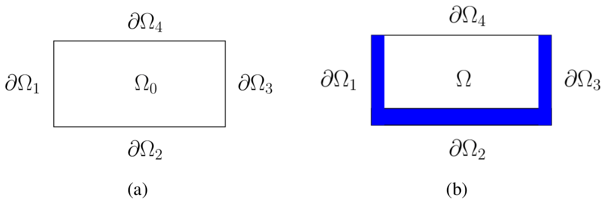
Figure 1(a) Limited domain representation, with . (b) Extended domain representation, , with absorption or sponge regions (of lengths Lx and Lz) highlighted in blue. ∂Ωi, , indicates the outermost boundaries of the full domain.
2.2 Gradient of misfit function
As mentioned in the first part of this section, in FWI the goal is to minimize the misfit function, which can be measured by Eq. (1). Typically, this minimization is carried out by employing a local optimization method. Thus, it is necessary to obtain the gradient, ∇mI(m), which may be computed efficiently by the adjoint method (Plessix, 2006). The adjoint-based gradient is achieved by using an augmented functional, also referred as Lagrangian functional. In the current case, it is given by the following:
where , m=m(x), and is the Lagrangian multiplier.
For a local minimum, the gradient of ℒ with respect to u, u†, and m should vanish. The gradient of , with respect to m, can be computed by the following:
where m′ is a perturbation of the parameter m.
2.3 Adjoint equation
In Eq. (4), we observe that the gradient ∇mI(m) depends on the adjoint variable u† that is computed by solving the adjoint wave equation, as follows:
For the domain Ω0 illustrated in Fig. 1a, the adjoint wave equation must satisfy the following boundary conditions: , for with , and , for . The adjoint wave equation is reversed in time. In this way, the initial condition is given by .
The adjoint wave equation is obtained by carrying out the gradient of with respect to the state variable u. Details of the method to obtain it can be found in the works of Plessix (2006) and Fichtner (2006).
3.1 Domain extension
For all the methods that we described here, we consider an extension of the spatial domain given by , in which an absorption region or sponge layer is added to the original spatial domain, . The absorption region is composed by two bands of length Lx, at the beginning and end of the domain in the direction x, and of a band of length Lz, at the end of the domain in the z direction. Again, ∂Ω denotes the boundary of Ω. Figure 1b shows the extended domain Ω, with the absorption region highlighted in blue. This kind of extension represents the typical configuration for seismic problems.
3.2 Damping
The method called damping was proposed initially by Sochacki et al. (1987), and it is a very simple way to reduce the spurious reflections of wave propagation in limited domains. The basic idea is to extend the original domain by adding a sponge layer to it, like the one in Fig. 1b, and then to introduce a damping term into the original wave, as in Eq. (2), such that it only affects the added layer. The resulting damped acoustic equation is given by the following:
where the acoustic wave Eq. (2) has been modified by the introduction of the damping term ζ(x)ut(x,t), with ζ(x) being nonzero only within the absorption region. That is, it should grow smoothly across the absorption bands from zero to its maximum at the outermost boundary. One may still impose the same initial and boundary conditions defined in the previous section.
Sochacki et al. (1987) proposed various alternatives for the damping function, ζ(x), including linear, cubic, or exponential forms. In general, all of them share a similar characteristic in that they vanish identically throughout the interior domain Ω0, while growing within the added bands from zero toward the outer boundary ∂Ω. We define the pair of functions ζ1(x) and ζ2(x) as follows:
so that the actual damping function ζ(x) is given by the following:
where cmax denotes the maximum velocity of propagation of c(x), and Δx and Δz are the discrete cell sizes of the spatial domain, respectively, in the x and z directions.
3.3 Perfectly matched layer
The method called perfectly matched layer (PML) has several formulations in the literature, considering the acoustic (second-order equation or first-order system formulations) and elastic cases. Like the damping method, the PML is widely used in seismic problems, particularly due to its efficacy in reducing spurious reflections in limited domains and for being more effective than the damping method. The formulation we present here have been proposed by Grote and Sim (2010) for the second-order form of the wave equation in the second-order equation.
The reasoning is similar to the damping method in that the sponge layers extend the original domain, like those in Fig. 1b. Additional terms are also introduced into the original wave in Eq. (2), which only affect the sponge layers, but now there are two of them, and they have their own evolution equations.
The two auxiliary functions provide adequate damping of the wave reflections by using similar terms to those of the damping method. The design of the method is such that it would ideally suppress all reflections in a continuous setting. However, some reflections may remain for a finite difference discretization, although they are strongly attenuated.
The full set of equations for the acoustic wave propagation with PML, along with the auxiliary functions, is given by the following:
Here, ϕ1(x) and ϕ2(x) represent the auxiliary variables, which are nonzero only in the absorption region. The notation ϕi,t indicates the partial derivative of ϕi, , with respect to the variable t, and is similar for the variables x and z, respectively, with ϕi,x and ϕi,z. The damping functions ζ1(x) and ζ2(x) are defined as in the damping method. The auxiliary functions will also be kept at zero over all the outer boundary of Ω.
When discretizing the PML equations, we position different variables on different places of the grid, dislocating by half grid size or half temporal step, in a so-called staggering of variables, as done in Grote and Sim (2010). Spatial variables for the auxiliary functions ϕ1 are staggered in the x direction and ϕ2 staggered in the z direction, as shown in Fig. 2. This staggering is convenient, considering that the centred discretization adopted here for the partial derivatives of those functions. As a result of this, u must be staggered in the directions of the partial derivatives in the evolution equations of ϕ1 and ϕ2. Conversely, ϕ1 and ϕ2 should be staggered in the directions of the partial derivatives in the evolution equation of u.
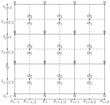
Moreover, some variables are also staggered in time, thus being defined at intermediary time instants. As a final result, the variable u(x,t) is taken as nonstaggered (co-located) in space, whereas ϕ1(x,t) and ϕ2(x,t) are staggered, and the functions ζ1(x), ζ2(x), c(x), and f(x,t) are staggered in Eq. (10) and nonstaggered in the Eqs. (11) and (12), when they appear in those equations. Therefore, when updating u(x,t), we employ the averages of the neighbouring values of ϕ1(x,t) and ϕ2(x,t), so that we have them on the nonstaggered grid. On the other hand, when updating ϕ1(x,t) and ϕ2(x,t), we average the neighbouring values of u(x,t) to define it on the staggered grid.
3.4 Convolutional perfectly matched layer
Although the PML method is usually very efficient for reducing boundary reflections, there are situations, such as in the presence of grazing waves, in which it is less effective. The convolutional perfectly matched layer (CPML) has been proposed as an improvement over PML, which should reduce the late time, low-frequency wave reflections and provide better absorption of grazing waves. In the case of the acoustic wave equation, the CPML is generally derived for the first-order set of partial differential equations (PDEs), but here we adopt the formulation proposed by Pasalic and McGarry (2010), which was designed for the second-order form of the wave equation.
The rationale is similar to the PML, in that one extends the original domain by adding a sponge layer to it (Fig. 1b). However, now one introduces four auxiliary functions into the original wave in Eq. (2). These functions also have their own evolution equations and can only affect the absorbing layer, just as in the previous approach.
The four auxiliary functions should provide adequate damping of the wave reflections by using similar terms to those of the PML. They consist of weighed combinations of the displacement and the auxiliary functions themselves. By design, the method should ideally suppress all reflections in a continuous setting, including those situations where the PML method fails.
The main equation reads as follows:
The auxiliary functions are updated by discrete in time relations (from time tn advancing a time step size of Δt, leading to tn+1) as follows:
where we have again used the notation for partial derivatives with a double subindex, as in ψ2,z, meaning that the second component of ψ is differentiated with respect to the z variable. The weighting factors for the auxiliary functions are given by the following:
The four auxiliary functions are only nonzero within the absorption region, while the functions ζ1(x) and ζ2(x) are defined as in the damping method. The constants can be chosen according to the problem.
3.5 Hybrid absorbing boundary condition
The last class of ABCs to be discussed here is termed the hybrid absorbing boundary conditions (HABCs). They can be interpreted as a combination of pointwise absorbing boundary conditions (ABCs) and domain extensions (like sponge layers), justifying the terminology of a hybrid method.
It is possible to use ABCs that do not require a domain extension enforced as pointwise boundary conditions, as suggested by the A1 Clayton condition (Clayton and Engquist, 1977) and the schemes by Higdon (1986, 1987). While these demand very little in terms of computational cost, they can still be prone to spurious reflections if used on their own. However, they can be effective if used in a hybrid way, in combination with domain extensions, as we illustrate below.
Clayton's A1 boundary condition (Clayton and Engquist, 1977) is based on a one-way wave equation (OWWE). This simple condition is such that outgoing waves normal to the border would leave without reflection. At the ∂Ω1 part of the boundary, the condition is as follows:
At ∂Ω3, the condition is as follows:
At ∂Ω2, the condition is as follows:
where we have explicitly expanded the spatial domain variable in its components ().
The Higdon boundary condition (Higdon, 1986, 1987) can take into account additional incidence directions and not only the normal direction as in Clayton's A1 condition. The scheme, termed to be of the order of p∈ℕ, is given at ∂Ω1 and ∂Ω3 by the following:
This also occurs at ∂Ω2, as follows:
This method ensures that outgoing waves with an angle of incidence at the boundary equal to αj present no reflection. The method we use in this work employs order 2 (p=2) and angles 0 and .
To combine these schemes with sponge layers, thus leading to hybrid schemes (HABC), we also extend the spatial domain, as shown in Fig. 1b. The difference with respect to previous schemes is that this extended region will now be considered as the union of several nested gradual extensions. As represented in Fig. 3, we define a region AM=Ω0, and the regions will be defined as the previous region, Ak+1, to which we add one extra grid line to the left, right, and bottom sides of it, such that the final region A1=Ω.
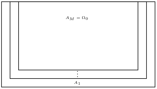
Figure 3Nesting of domains for the hybrid ABC method. The full region A1 is equivalent to Ω.
To illustrate how the HABC is used, we will describe the process of how we obtain a solution using the usual solution of acoustic wave equation together with the absorbing conditions showed in A1 and Higdon schemes. First, assume is known at instant t−Δt in all the extended Ω domain. We then update one time step from the solution to u(x,t) using the usual acoustic wave equation over Ω, with the null Dirichlet or Neumann boundary conditions defined for ∂Ω.
Now, for each region Ak, with k going from the innermost domain AM to the outermost domain A1, we construct an auxiliary functions, uk(x,t), based on the current solution, u(x,t), by applying the absorbing condition A1 or Higdon for the domain (Ak). For finite difference schemes, this implies altering only the values of u(x,t) at the border of Ak, i.e. on ∂Ak, to obtain uk(x,t). The final solution for each region Ak, which will be the input solution for region Ak−1, will be given by a convex combination between uk(x,t) and u(x,t), as follows:
where wk is a weight function that grows from zero at to one at , and will be used as the new u(x,t) for the next region (Ak−1). In summary, we loop over the nested regions, from the innermost to the outermost, subsequently applying the pointwise A1 or Higdon boundary conditions and weighting them with respect to the a distance metric of each boarder from the innermost domain (defined by weights wk).
The particular weight function to be used could vary linearly or nonlinearly (Liu and Sen, 2018). We can choose a linear weight function, as follows:
Or, preferably, a nonlinear function could be used, as follows:
We take P=2, and we choose α, following Liu and Sen (2018):
-
, in the case of A1,
-
, in the case of Higdon,
where the value of npt designates the number of discrete points that define the length of the extended region in the direction x or z. In our experiments, we observed that HABC produces better results with a nonlinear weight function, but the choice of the type of weights can be adapted according to the application. Moreover, here we use the values for α proposed by Liu and Sen (2018), but the parameter can be adjusted for specific cases.
After introducing the different approaches of ABCs, this section presents the adjoint equations. The formulations and further details for all ABC methods investigated here are presented in Appendix A.
4.1 Damping
The adjoint wave equation with damping ABC method is given by the following:
This means that there is a self-adjoint wave equation, which satisfies the following boundary and initial conditions:
The index values are based on the boundaries illustrated in Fig. 1b.
4.2 PML and CPML
The adjoint wave equation with the employment of PML method reads as follows:
where the auxiliary functions and satisfy the respective auxiliary differential equations. This is demonstrated in the following:
For the CPML method, the adjoint wave equation is cast in the following form:
The auxiliary functions (, , , ) in the previous equation are given by the following:
The adjoint auxiliary equations and (i=1, 2) are solved recursively in adjoint/backward time t†, which is reversed with respect to the forward time t.
Again, it is possible to note that the resulting adjoint equations are self-adjointing with respect to the forward problem with PML and CPML. Both PML and CPML adjoint wave equations satisfy the boundary and initial conditions given by Eqs. (29)–(31).
4.3 Hybrid absorbing boundary condition (HABC)
On employing the HABCs methods, the adjoint wave equation is defined by Eq. (5), which satisfies the boundary condition at the free surface given by Eq. (30), and the initial condition reads as in Eq. (29). For the HABC-A1 method, the truncated boundaries, , have the following condition:
For HABC-Higdon, the boundary condition at reads as follows:
The boundary condition above is written in a general form. In this work, we employ in both forward and adjoint solver of the order of 2 (p=2) and with angles 0 and .
After setting the adjoint counterparts to Clayton's A1 and the Higdon boundary conditions, as shown in Appendix A3, the adjoint HABC approach is completed using a similar process of the forward problem. In summary, once the adjoint is solved inverse in time, we assume that is known at instant t+Δt in all the extended Ω domains. We update it to , using the usual adjoint acoustic wave equation over Ω, and then construct the auxiliary functions for each region, from AM to A1, applying the A1 or Higdon conditions for each region. As in the forward problem, we construct each update of the solution to the adjoint problem, at each region Ak, with a convex combination using a weight ωk, as follows:
where will be used as the new for the next region (Ak−1).
This derivation shows, once more, the self-adjointing nature of the adjoint problem with HABC-A1 or HABC-Higdon.
The numerical simulations were carried out using the Devito software (Louboutin et al., 2019; Luporini et al., 2018; Kukreja et al., 2016). According to its own website, Devito is a Python package that combines a domain-specific language (DSL) and a full code generation framework. It is especially geared towards the design of highly optimized finite difference kernels for its use in inverse problems. It makes use of SymPy to allow a symbolic definition of the operators at a high-level notation, and then it generates optimized code that is automatically tuned to specified computer architectures.
5.1 Coding framework
In general, symbolic computation is a powerful tool, as it allows users to build complex solvers in only a few lines of high-level code. However, the symbolic computation is usually impractical, from a computational performance point of view, for most complex applications. On the other hand, considering the compilation of a high-level symbolic solver into a highly optimized low-level code, with adjustable stencil discretization at the runtime, one should be able to develop computationally efficient methods that reduce the coding development time. This is the underlying goal of Devito. Here we highlight the main aspects that concern this work with respect to software development in Devito.
In this work, we use the main Devito backend as driver but implement all methods using only high-level symbolic methods available from Devito. This allows the methods to be easily modified by interested users. Our implementation is described in detail in the ABC Devito tutorials, available from the master branch of Devito (PML Jupyter notebook example can be found at http://nbviewer.org/github/devitocodes/devito/blob/master/examples/seismic/abc_methods/03_pml.ipynb, last access: 6 June 2022).
Due to the simplicity of working with symbolic equations, the code development can be accomplished with minor modifications of existing codes in Devito for a typical acoustic wave propagation. We highlight, in Fig. 4, the main implementation characteristics. The differential operators have a syntax related to their original structures, such as dt, dt2, dx, dz, and Laplace, for instance. Their corresponding finite difference approximations (Fornberg, 1988) can then be picked by the user among many available, or custom designed, schemes for each operator.
The creation of space-dependent (function), space–time-dependent (time function), and other types of fields is done as a preprocessing step. It amounts to setting the properties linked to that field such as, for instance, spatial order, temporal order, staggering type, and floating number type, among other specific properties of each field.
The term “op” described in Fig. 4 represents the time evolution operator for a given set of symbolic equations and is where all the backend compilations, optimizations, and running of Devito take place. At this point, a user defines a number of time steps and its size (dt). In that operator, one places the elements called stencils, which represent the differential equations that are applied to each particular subdomain. Furthermore, the op carries the natural boundary conditions (“bc”), forcing terms (src_term), and information about the receivers (rec_ term).
An important resource of Devito for ABCs is the possibility of partitioning the domain of interest into subdomains to which distinct attributes can be assigned. The additional PDEs originated from the ABC methods of PML, CPML, and HABCs were solved only in the extended domain (blue region), as exemplified in Fig. 1, considering their particular structure. In the case of the damping, PML, and CPML methods, the pure acoustic wave equation was solved in the main domain (white domain), and the modified acoustic wave equation, that is, the equation that includes auxiliary functions and/or damping functions, and the equations for the auxiliary functions, are solved only in the extension (blue region) where they really are required. In the case of HABC methods, as we showed before, we solved the pure acoustic wave equation over all the domains (white and blue region), but the additional equations for the boundaries are solved only in the extension domain (blue region), to be later combined with the original solution through a convex procedure, as was previously described. The possibility of creating specific subdomains allows us to save time and memory for the computations.
5.2 Computational performance
Devito uses Python as frontend, to allow for ease of code development, and C/C as backend language for an optimized computational runtime. Architecture-dependent optimizations are possible and so are parallel distributions of the task. To date, Devito allows parallelization with OpenMP (DEVITO_LANGUAGE=openmp), MPI (Message Passing Interface) (DEVITO_MPI=n, where n is the number of nodes), and some compilation support for general-purpose computing on graphics processing units (GPGPUs).
In this work, simulations have been executed on the Mintrop HPC (high-performance computing) cluster, at the University of São Paulo. The computational executions were carried out on an asynchronous module definition (AMD) node, which has dual sockets AMD EPYC 7601 is clocked at 2.2 GHz, with 64 cores and 512 GB of DDR4 (double data rate 4) memory.
In FWI executions, the sources of shot waves ran in parallel with the computing library Dask (http://docs.dask.org/en/latest/, last access: 8 July 2022), where the number of tasks was equal to the number of sources. Only OpenMP was activated to solve the partial differential equations (PDEs) in parallel in the Devito framework. The executions were performed by using the C compiler, GCC 8.3.0.
Computational performance (wall clock runtime and memory usage) was measured using the Dask diagnostic performance tool.
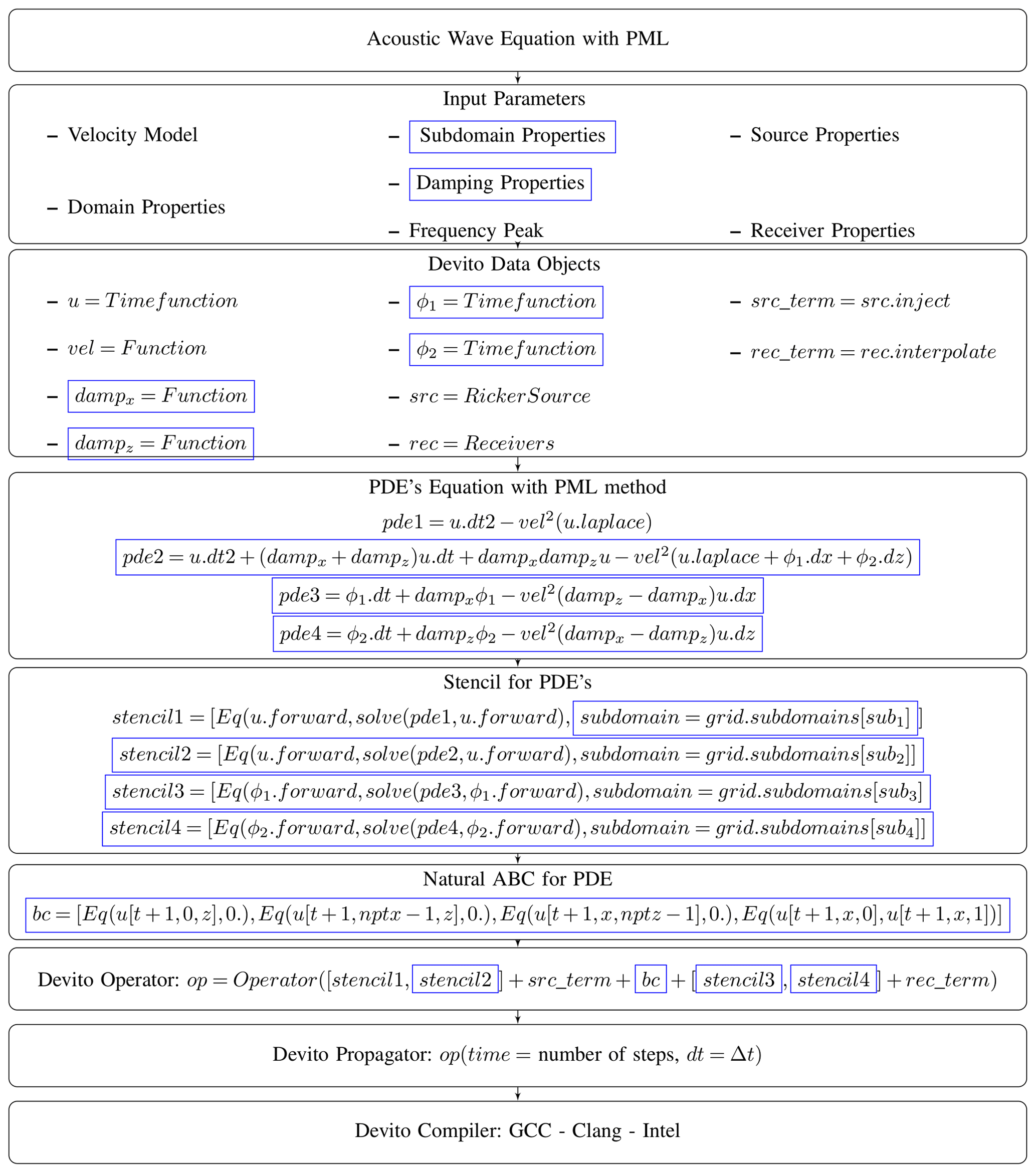
Figure 4Example of logical implementation of PML method in the Devito coding framework. The diagram is similar to that of the original Devito development paper (Louboutin et al., 2019), but we highlight in blue boxes the kind of changes required for a PML implementation.
In this section, we assess the performance of the ABC methods on the forward and adjoint wave equations. In the literature, analyses of ABCs are usually limited to the homogeneous velocity model (Gao et al., 2017; Grote and Sim, 2010; Liu and Sen, 2012). Also, to the best of our knowledge, those conditions have not yet been assessed for their role in the adjoint problem. In the present work, we propose to do precisely that, i.e. to evaluate ABCs for heterogeneous velocity models and to do so for the adjoint problem as well.
The objective is to carry out the ABC analysis for the usual set-up adopted in a FWI problem, e.g. on considering heterogeneous velocity models. These are illustrated in Fig. 5, and they are, respectively, referred to as circle, horizontal layers, part of the Marmousi (Martin et al., 2006), and a 2D SEG/EAGE salt model (Aminzadeh and Brac, 1997). The placement of receivers and sources follows the usual configuration adopted in the literature to run a FWI case (Virieux and Operto, 2009), that is, the sources and receivers located closer to the free surface. Tables 1 present the numerical set-up that was used to run the analyses of both forward and adjoint solutions with the ABCs.
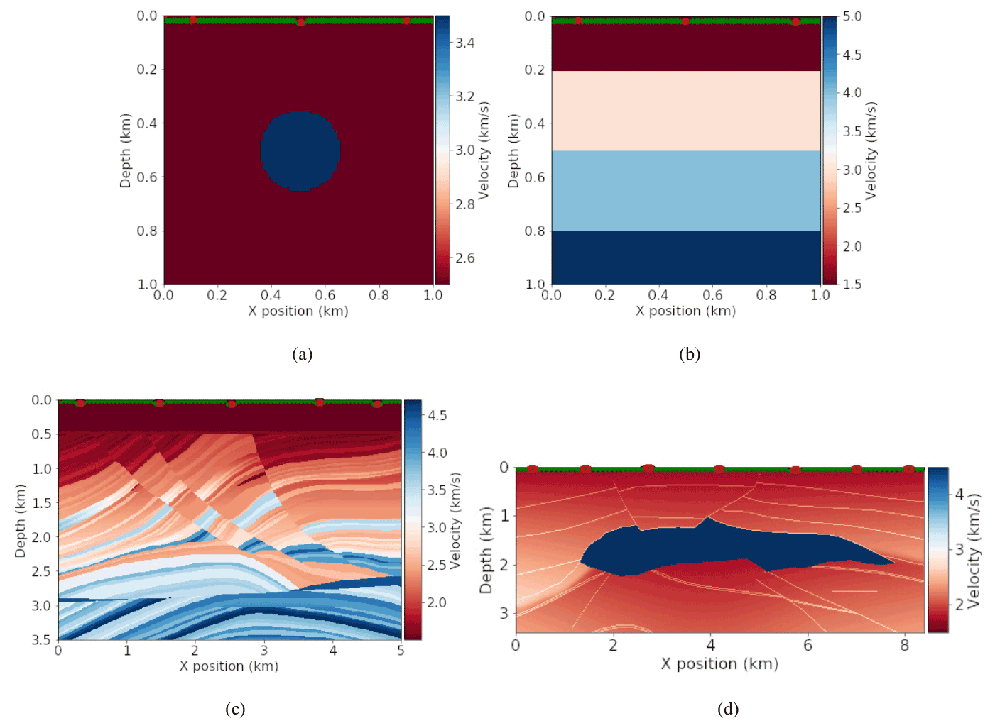
Figure 5Velocity models are shown as (a) a circle, (b) horizontal layers, (c) part of the Marmousi, and (d) the 2D SEG/EAGE. The red points illustrate the source positions, and the green points illustrate the receiver positions.
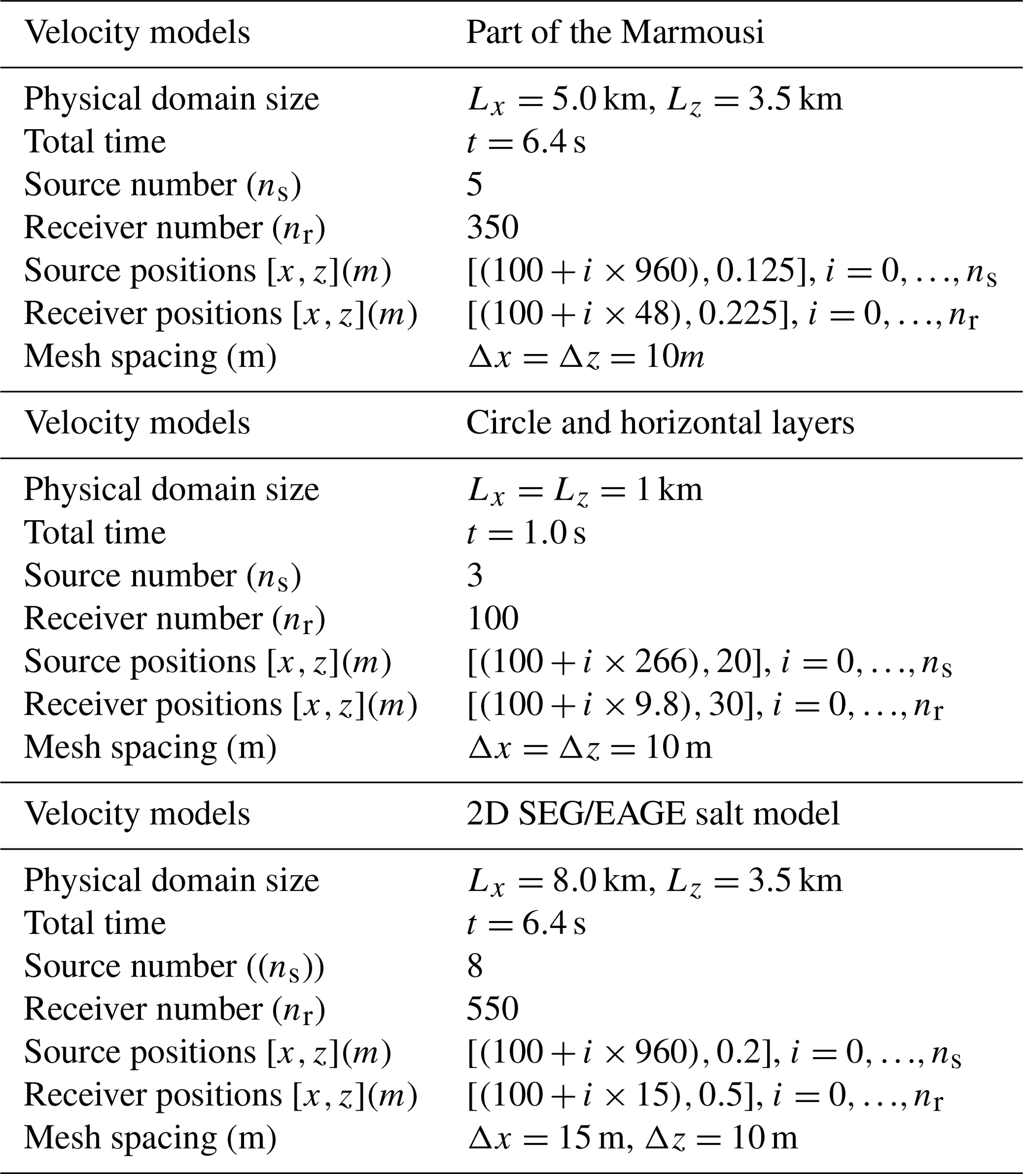
The evaluations of the ABC effectiveness in attenuating the reflections used reference fields designed to keep boundary reflections from ever reaching the actual domain of interest. To achieve this, the computational domain for the reference solution is extended, and the simulated time is set in such a way that neither the forward nor the backward waves have enough time to reach the outermost boundaries. Figures 6 and 7 show the reference solutions of the forward and adjoint solvers, respectively. In none of the cases did the waves have time to reach the truncated boundaries of , as illustrated in Fig. 1. Therefore, the reference fields that are used as a base for comparison are free of reflections. These extended regions should not be confused with the absorbing layers used for the boundary schemes tested here. The goal of this particular and very large extended region is solely to define adequate reference solutions with no inbound reflected waves.
The reference solutions used to evaluate the ABC effectiveness in attenuating the reflections are referred to here as the accuracy references, and these will be used to compute the quantitative error, given by the following expression:
which computes the relative error of the forward/adjoint solution (), using ABC, with the corresponding one in the reference field on the physical (inner) domain of interest (Ω0). The variables sref(x,tf) and s(x,tf) represent, respectively, the accuracy of the reference solution and that which has made use of a particular ABC. The value tf is the final time of the simulation.
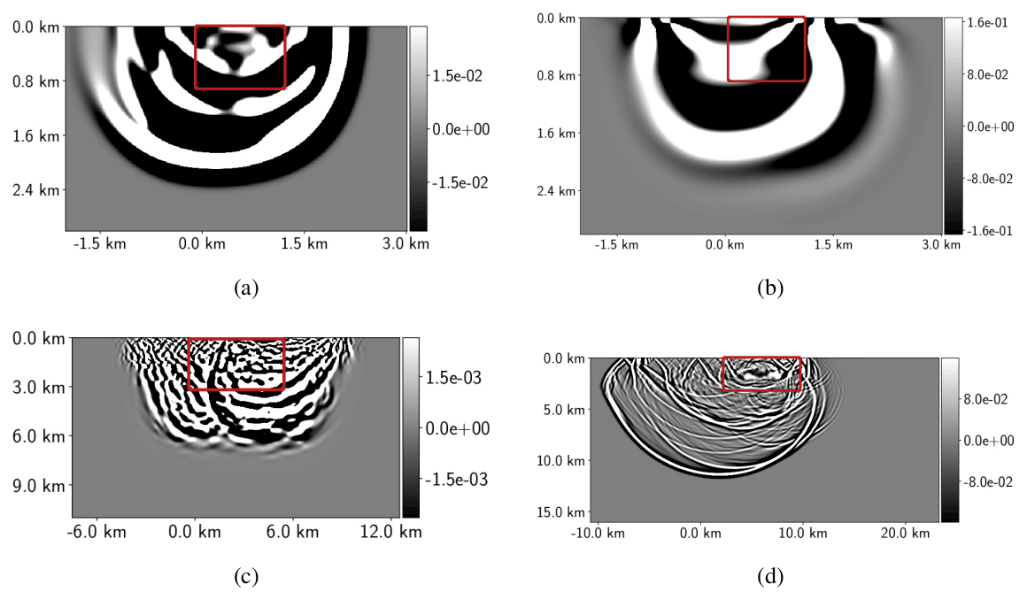
Figure 6Reference solutions of the forward wave equation (u). (a) Circle velocity model at t=1 s. (b) Horizontal layers velocity model at t=1 s. (c) Part of the Marmousi velocity model at t=6.4 s. (d) 2D SEG/EAGE salt velocity model at t=6.4 s. The regions inside the red square are the physical domains, with the red lines indicating the boundaries (∂Ω0), and the regions outside are the extended domains.
Figure 7Reference solutions of the adjoint u† wave equation related to the velocity models. (a) Circle velocity model at t=1 s. (b) Horizontal layers at t=1 s. (c) Part of the Marmousi velocity model at t=6.4 s. (d) 2D SEG EAGE salt model at t=5 s. The regions inside the red square are the physical domains, with the red lines indicating the boundaries (∂Ω0), and the regions outside are the extended domain.
The ABCs were applied to domain extensions defined in terms of the physical domain length in x direction, . The extension width lw was set as a percentage p of lx, i.e. . Moreover, the same extension lw applies to the depth of the domain in the z direction. The range of p was taken to be . Previous works (Gao et al., 2017; Liu and Sen, 2018) have taken the number of points in the domain extension pne, instead, as a measure of its size. Then, pne was picked for between 5 % and 10 % of the number of points in the physical domain. However, that also meant an extension between 5 % and 10 % of the original domain length, since square domains with uniform grid spacing were usually adopted to carry out the analyses (Gao et al., 2017; Liu and Sen, 2018). Therefore, the range of domain extensions here is consistent with that of previous works.
To exemplify the choice of lw, we consider the domain of the circle velocity model (plotted in Fig. 5a). In this case, lx=1 km and, at p=2, the width . At p=2, the extended domain has the width lw=20 m in the x and z directions, which means pne=2 for the mesh grid m.
In the extended domain, the velocity model c was built by employing a constant extrapolation of the physical values of c in the boundary points and z=zF, x=xI and , and x=xF and .
6.1 Forward wave equation
As a first step, a fixed lw and various frequency peaks f of a Ricker wavelet are considered for an error analysis. The extended domain width was chosen to keep the major portion of the curves log 10E(uref,u) below 1, where E(uref,u) is given by Eq. (33).
Figure 8 depicts . In essence, it shows that the frequency peak bears on the effectiveness of the ABC methods. One notices in Fig. 8c and d that, for more realistic velocity models (part of the Marmousi and 2D SEG/EAGE salt models), the error grows with f for the PML, CPML, and HABC-Higdon. For simpler models, such as the circle and the horizontal layers, the error also exhibits a slight growth but only for the PML and CPML methods. It is also clear in Fig. 8 that the HABC-Higdon incurs smaller errors. For the more realistic models, PML and CPML have come closer to HABC-Higdon results, whereas the damping method consistently exhibits the highest errors.
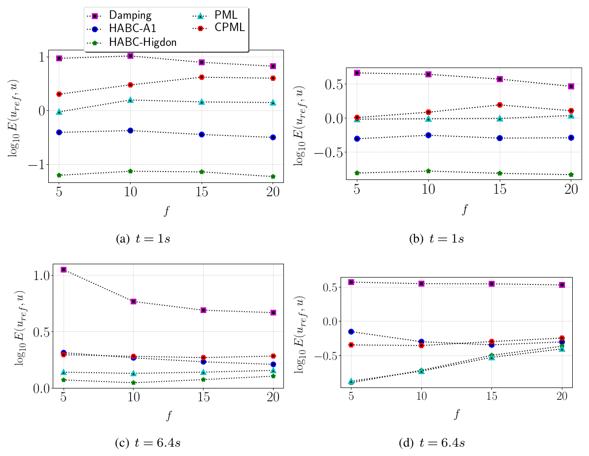
Figure 8Error curves of the forward solution (u) with respect the frequency peak f of Ricker wavelet. The analyses considered the wave solutions for the velocity models, including a circle (a), a heterogeneous model built with horizontal layers (b), part of the Marmousi model (c), and the 2D SEG/EAGE salt velocity model (d).
In order to ascertain whether similar behaviour would be seen for different sizes of domain extension, the next test assesses the ABC performance as a function of lw. On accounting for the previous evidence of the peak frequency f effects upon performance, this test only includes the more realistic models, namely the part of the Marmousi and the 2D SEG/EAGE salt models.
Figure 9 depicts log 10E(uref,u) as a function of p and the lw thereof. The errors decrease as p increases. Once again, the relative errors grow with f for PML, CPML, and HABC-Higdon alike. This behaviour is observed in both Marmousi and 2D SEG/EAGE salt velocity models. On the other hand, the errors decrease as f grows for the damping method. The damping and HABC-A1 errors approximate those of the other ABCs (PML, CPML, and HABC-Higdon) as f grows, especially for the part of the Marmousi model. Figure 9a shows that the PML and CPML errors are much closer to each other, whereas in the 2D SEG/EAGE salt model, Fig. 9b shows that PML has a lower error than that of the CPML. In all cases, the HABC-Higdon incurs errors that are either similar to or smaller than those of the PML and CPML, while those of the damping method are the highest.
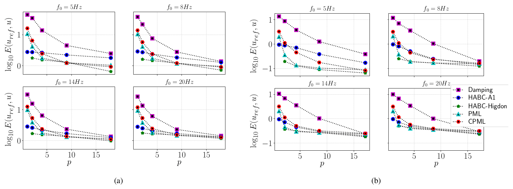
Figure 9Error curves of the forward solution (u) with respect to p (percent of Lx) for different peak of frequency f0. The analyses considered the wave solutions for the velocity models, i.e. (a) part of the Marmousi model and (b) 2D SEG/EAGE salt model.
6.2 Adjoint wave equation
The previous section presented analyses of the ABC performance in the context of the forward wave equation. Here, we consider their performance in the adjoint wave equation, which is referred to as the backward problem.
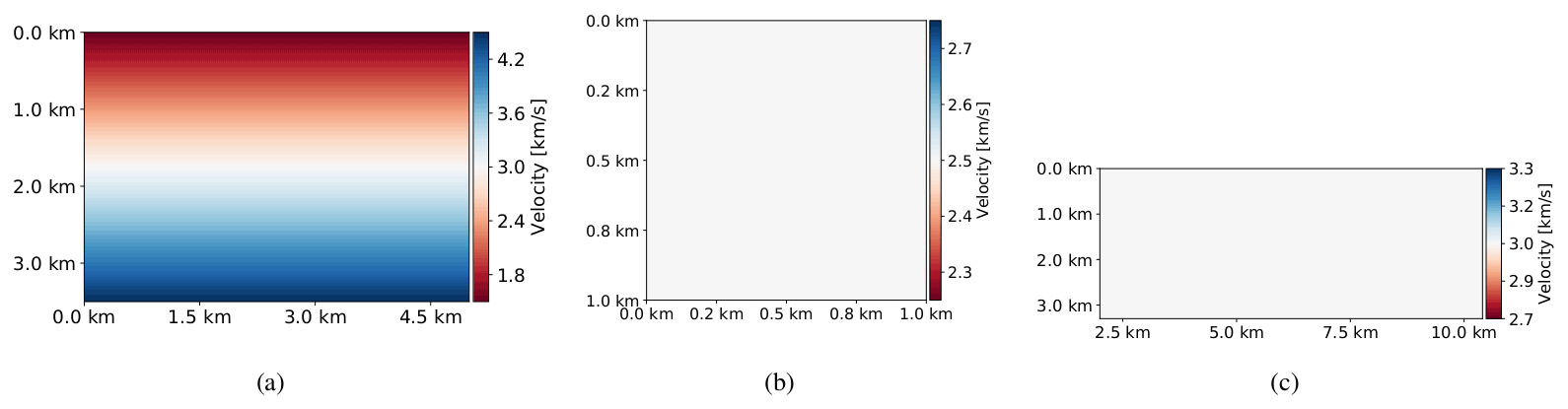
Figure 10Initial guess of velocity model. (a) Part of the Marmousi (linear initial guess model). (b) Circle and horizontal layer velocity models (constant initial velocity of 2.5 km s−1). (c) 2D SEG/EAGE salt model (constant initial velocity of 3 km s−1).
The adjoint forcing term is given by . In that expression, uobs represents the observed, recorded data from the true velocity model, whereas u stands for an initial velocity model – henceforth termed the guess velocity model. Any nonzero difference between them and the forcing term, d, will give rise to a nontrivial solution. Hence, in the analysis that follows, uobs is based on the models shown in Fig. 5 (true velocity), while u is computed from the models shown in Fig. 10 (guess velocity).
The following steps are taken to assess the adjoint ABC performance: a reference adjoint solution is computed in the reference enlarged domain to avoid spurious reflections, and next, adjoint solutions subject to the various ABCs are computed, and their errors with respect to the accuracy reference are evaluated by Eq. (33). Figure 11 shows the curves of . In 2D SEG/EAGE velocity model, the PML, CPML, and HABC-Higdon errors grow with f. Somewhat surprisingly, the errors come closer than those of the damping method for higher values of f, as shown in Fig. 11d. In the circle velocity model, Fig. 11a shows only the PML and CPML errors growing with f. In several cases, HABC-Higdon errors are either close to or smaller than the PML errors. Figure 12 presents error curves with respect to the domain extension parameter p, for distinct frequency peaks f. In all cases, the error diminishes as p increases. For part of the Marmousi velocity model, Fig. 12a shows the PML, HABC, and damping errors dropping as f grows, whereas CPML errors rise with f. For 2D SEG/EAGE, Fig. 12b shows the ABC errors going up with f.
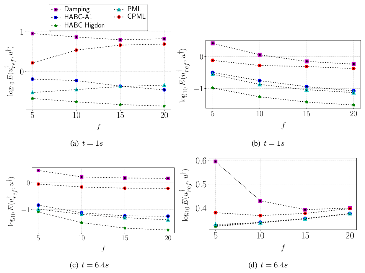
Figure 11Error curves of the adjoint solution u† with respect to the peak of the frequency. The tests consider the wave solutions for the velocity models, including (a) the circle, (b) a heterogeneous model built with horizontal layers, (c) part of the Marmousi model, and (d) the 2D SEG/EAGE salt model.
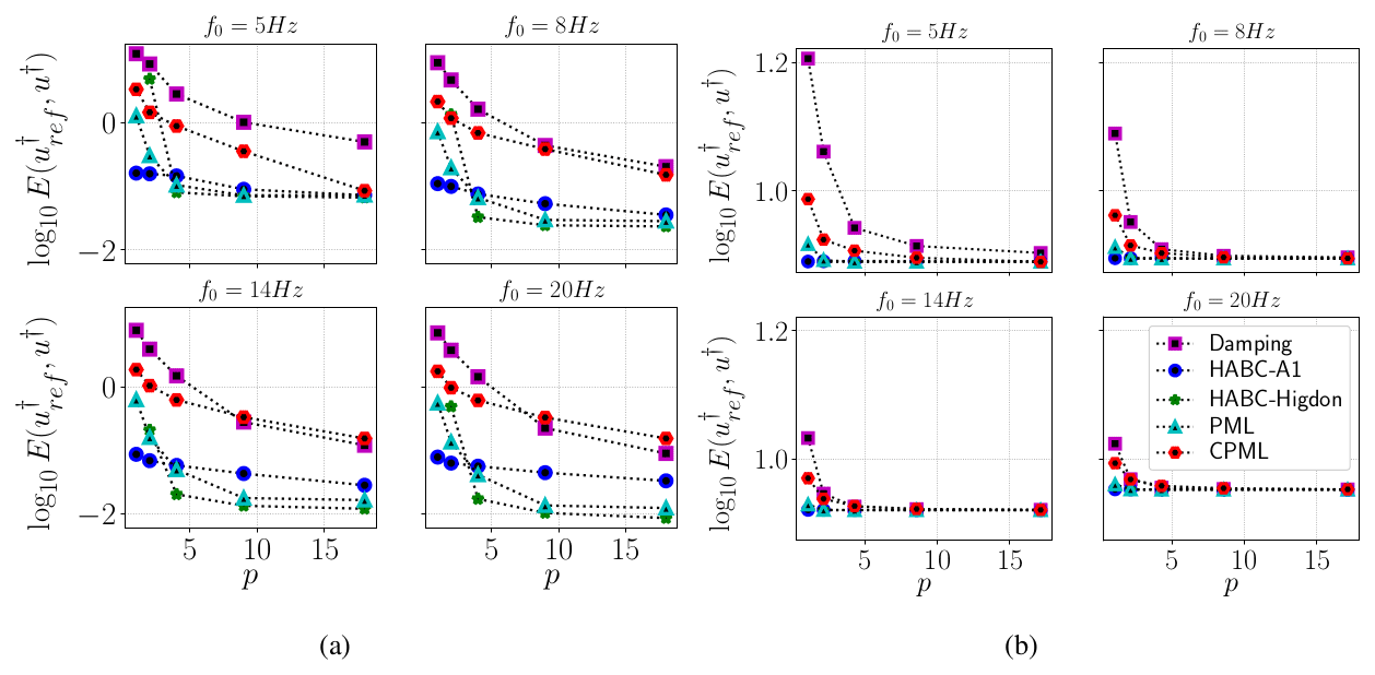
Figure 12Error curves of the adjoint solution u† with respect to p (percent of Lx) for different frequency peaks. The tests consider the wave solutions for the velocity models, including (a) part of the Marmousi model and (b) the 2D SEG/EAGE salt model.
Similar to the forward problem, the frequency peak f bears on the adjoint ABC effectiveness, as well. Moreover, the HABC-Higdon error has shown to be either smaller than or close to that of the PML. It also appears that the CPML has not been quite effective in the adjoint problem. That can be noted especially for part of the Marmousi velocity model, as its errors are the highest for higher frequency peaks f.
In conclusion, the adjoint problem experiences its own spurious boundary reflections, and those from the forward solution, which are carried over into the adjoint solution via the external forcing term. The latter depends on the forward wave solution (u) stored in the receivers, as can be verified in the adjoint equation shown in Eq. (1).
6.3 Computational cost: memory usage and time of simulation
Given the above diversity of ABC characteristics, a question naturally arises as to their computational costs and memory usage. This section addresses precisely those topics. To that end, the range was adopted to run the forward solver, subject to the ABCs. Part of the Marmousi was the chosen velocity model for the experiments, with the set-up shown in Table 1. Section 5.2 describes the settings, as libraries and machines, used in the computational performance measures.
Table 2 shows the average wall clock runtime of simulations and the memory usage of a computational reference case, which used homogeneous Dirichlet boundary conditions (Eq. A3), and no ABCs were employed. That is, the tests were performed in the physical domain Ω0 only, without any extensions. Such a case is henceforth referred to as the no-ABC case, and it is used as a computational reference to evaluate the growth of the memory usage and the wall clock time of the cases that are subjected to the various ABC methods.
Figure 13a and b present the results of such comparison in the form of a relative increase in percentage of the time of simulation tg and memory usage mg of the ABCs, as compared to the no-ABC reference. Figure 13a shows that the growth of memory usage associated with the damping method remains below 5 % within the whole range of the domain extensions, p. However, as noticed in Fig. 14a and b, curves of and present the highest errors when the damping method is employed.
The CPML method is far more expensive, due to the number of additional variables to be solved. At p≈1, Figs. 13a and b show the memory usage increasing by more than 10 %, while time of simulation grows by more than 80 %. On evaluating and , Fig. 14a and b show that the CPML errors are close to the PML errors, but the CPML computational performance has been more expensive than the PML.
The HABC methods are more expensive than the damping, but they have shown to attain lower values of mg and tg than those of the CPML and PML. In all cases, HABC-Higdon requires more time and memory usage than HABC-A1. However, Fig. 14a and b depict the errors of HABC-Higdon as being smaller than that HABC-A1 errors for p>1. Also, for p>1, HABC-Higdon demands less wall clock time and memory usage than that of PML and CPML, whereas its performance in decreasing the reflections (measured by log 10E(uref,u)) has been similar.
Table 2Computational cost related to the execution of the forward solver when there is no employment of any ABCs methods. The velocity model was part of the Marmousi, with the settings shown in Table 1.
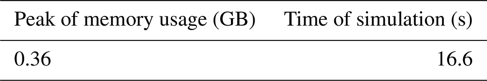

Figure 13The percent growth of memory usage (a) and time of simulation (b), as compared to the no-ABC case. The measures are related to the execution of the forward solver. The velocity model was part of the Marmousi, with the settings shown in Table 1.

Taking into account the effectiveness plus the computational time and memory usage, one observes that HABC-Higdon is a proper choice to be employed in an FWI execution. However, the damping method has presented a time of simulation and memory usage that is much smaller than the other ABCs. Besides that, the PML method is commonly employed in FWI works (Abubakar et al., 2009; Asnaashari et al., 2012; Aghamiry et al., 2019; Ben-Hadj-Ali et al., 2011). Therefore, this section proposes to compare numerical results and the computational cost in FWI using damping, PML, and HABC-Higdon.
The FWI applications take the Marmousi as the true model. True receiver signals are obtained in the accuracy reference field, where the domain was extended to avoid spurious reflections.
The set-up used to run this FWI case is presented in Table 3. The Marmousi velocity model and the initial model are, respectively, illustrated in Fig. 16a and b. The first case evaluates the ABCs performance in FWI for a fixed peak of frequency f0=7 Hz. The simulations were executed using the time step of 0.001 s. A subsampling approach with sampling ratio of r=5 was employed, which satisfies the Nyquist criterion for peak of frequency f0=7 Hz and a time step of 0.001 s. The search algorithm is the L-BFGS-B (Byrd et al., 1995), where the stop condition was the number of iterations. The extended domain width lw was set according to Kaltenbacher et al. (2013), i.e. km (equivalent to p≈4).
Figure 15 shows the misfit and the error of the velocity model Ec of the FWI runs. In particular, the error Ec was computed by the following expression:
where ctrue is the true velocity model, and ccomp is the computed velocity model provided by the FWI run. To evaluate Ec, the velocity models ctrue and ccomp were both defined in the same mesh set-up.
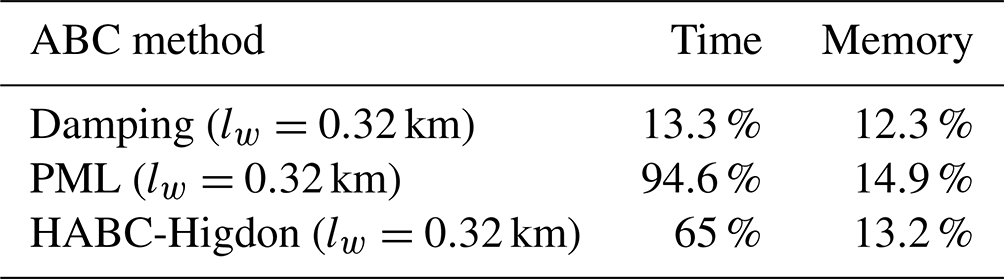
On comparing the performance of the HABC-Higdon to that of the PML, the results in Figs. 15 show smaller values of I(m) and Ec for the former. Furthermore, Table 4 shows that the percent growth of memory usage and the wall clock time related to the HABC-Higdon required significantly less time and a slightly smaller memory usage compared to the PML. The reason for this better performance is basically due to the fact that the HABC-Higdon does not require additional variables and equations to be solved, which incur in both added computational time and memory usage. Therefore, it is proper to conclude that HABC-Higdon has shown better overall performance compared to PML.
Comparing the HABC-Higdon with respect to the damping scheme, we note that the damping scheme with the same damping layer size as used in the HABC-Higdon (lw=0.67 km) is considerably faster and uses less memory (see Table 4). This is mainly due to the computational overhead of HABC-Higdon having to successively apply boundary conditions in nested domains, with added memory use due to a few auxiliary variables used in this nesting procedure. However, Fig. 15 shows that I(m) and Ec of the HABC-Higdon (with lw=0.67 km) are lower than those of the damping, with the damping scheme requiring a much larger damping layer to reduce the error. Particularly in Fig. 15b, it is clear that, even when increasing lw, the damping error Ec is still higher than that of the HABC-Higdon. Moreover, Table 4 shows that the percent growth of wall clock time of simulation and memory usage of the damping method with lw=2.5 km is significantly larger than that of the HABC-Higdon results with lw=0.67 km. Therefore, HABC-Higdon advantages seem twofold, in that it combines a good performance in mitigating spurious reflections with a relatively low computational cost.
Table 3Set-up used to carry out the numerical FWI simulations, which are used to compute the velocity models that are then matched with Marmousi.
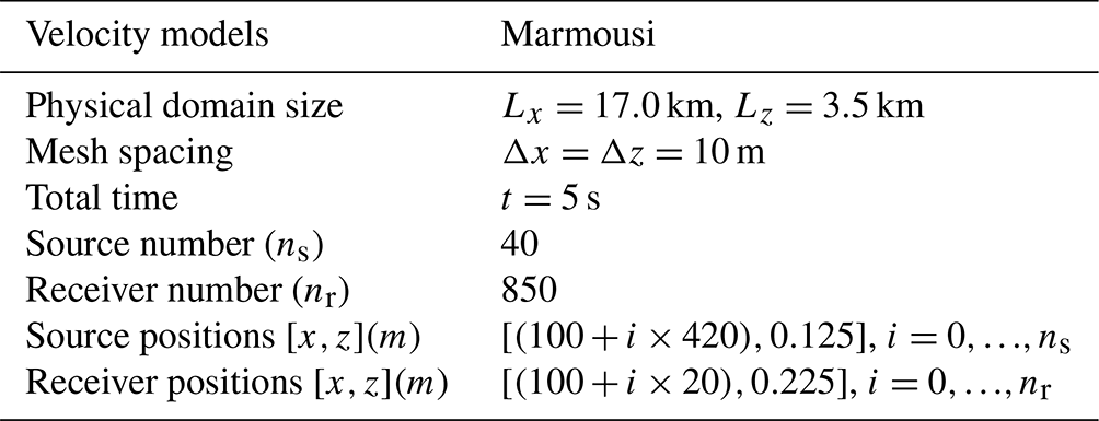
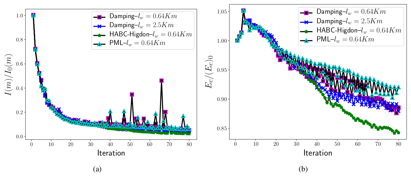
Figure 15Comparisons of the misfit values (a) and of the velocity model errors (b) for a velocity model computation that is then matched with Marmousi, where I0(m) and (Ec)0 are the values obtained at the first iteration.
Table 4The percent growth of the wall clock time and RAM usage, as compared to the no-ABC case (lw=0.0 km). The measures are related to a source of a single shot wave of the FWI execution for the velocity model that is matched with Marmousi. In this case, the execution of FWI with no-ABC required 75 s of wall clock time and 5 GB of memory usage.


A second case considers the peak of frequency f0=15 Hz and applies the multiscale approach in frequency (Bunks et al., 1995). The numerical set-up is displayed in Table 3. The cuts of the frequencies are fc=3 Hz, fc=5 Hz, and fc=8 Hz. The extended domain choice was based on the peak of frequency f0=15 Hz. Therefore, the extended domain had km (equivalent to p≈2). The initial velocity model used in the FWI executions is displayed in Fig. 16b, and r=4 was set in the subsampling approach (also satisfying the Nyquist criterion for peak of frequency f0=15 Hz and time step 0.001 s). Figures 17 and 18 present the misfit and the error of the velocity model, and Fig. 19 shows the computed velocity model for the FWI solver with HABC-Higdon. Once again, FWI with the damping methods has shown the worst performance, as the misfit values and the velocity errors are the highest. FWI executions with HABC-Higdon and PML have presented a similar performance. Differences are observed in the velocity errors Ec, and Fig. 18a shows smaller errors associated to HABC-Higdon for a cut of the frequency fc=3 Hz. Whereas, for fc=5 Hz and fc=8 Hz, the Ec associated to the PML method has been smaller.
Once again, on evaluating the performance in mitigating the reflections and the computational cost that is presented in Table 5, one verifies the HABC-Higdon as a proper choice to be employed in an FWI execution.
Figure 16c shows the computed velocity models when the HABC-Higdon was employed. However, FWI executions were performed for all ABC methods. The computed velocity models were similar, mainly when PML, CPML, and HABCs methods were applied. FWI with the damping method was more affected by the reflections originating in the truncated boundaries. In this case, the field of the computed velocity model was the furthest from the Marmousi model. Regarding the quantitative comparisons, the computed velocity model errors (Ec) related to the HABC-Higdon have remained the smallest.
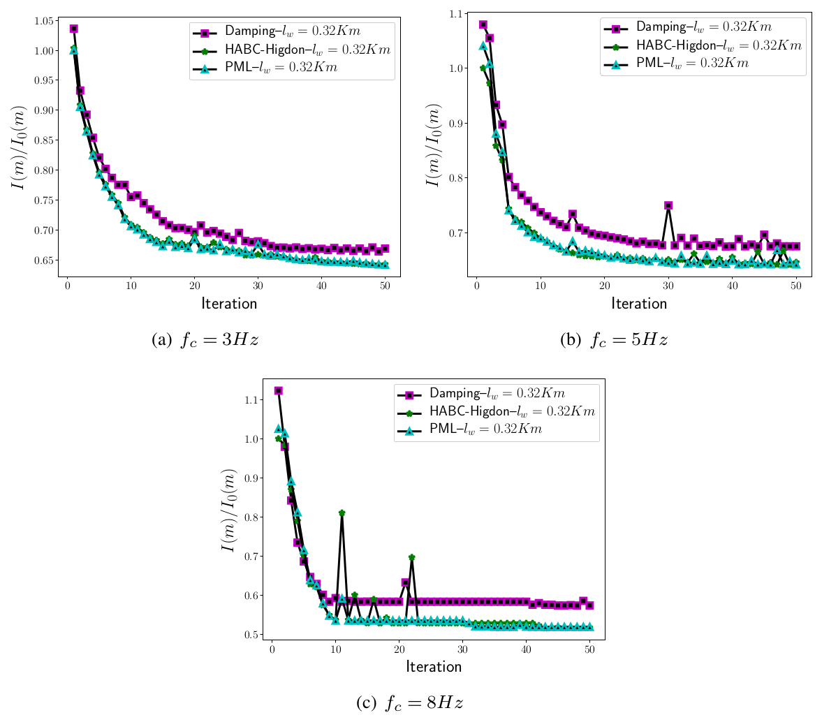
Figure 17Comparisons of the misfit values for a velocity model computation that is then matched with Marmousi, where the peak of frequency is f0=15 Hz, and a multiscale approach in frequency (Bunks et al., 1995) is employed. I0(m) is computed at the first iteration, which is the minimal misfit value given by the employment of the damping, HABC-Higdon, and PML methods.
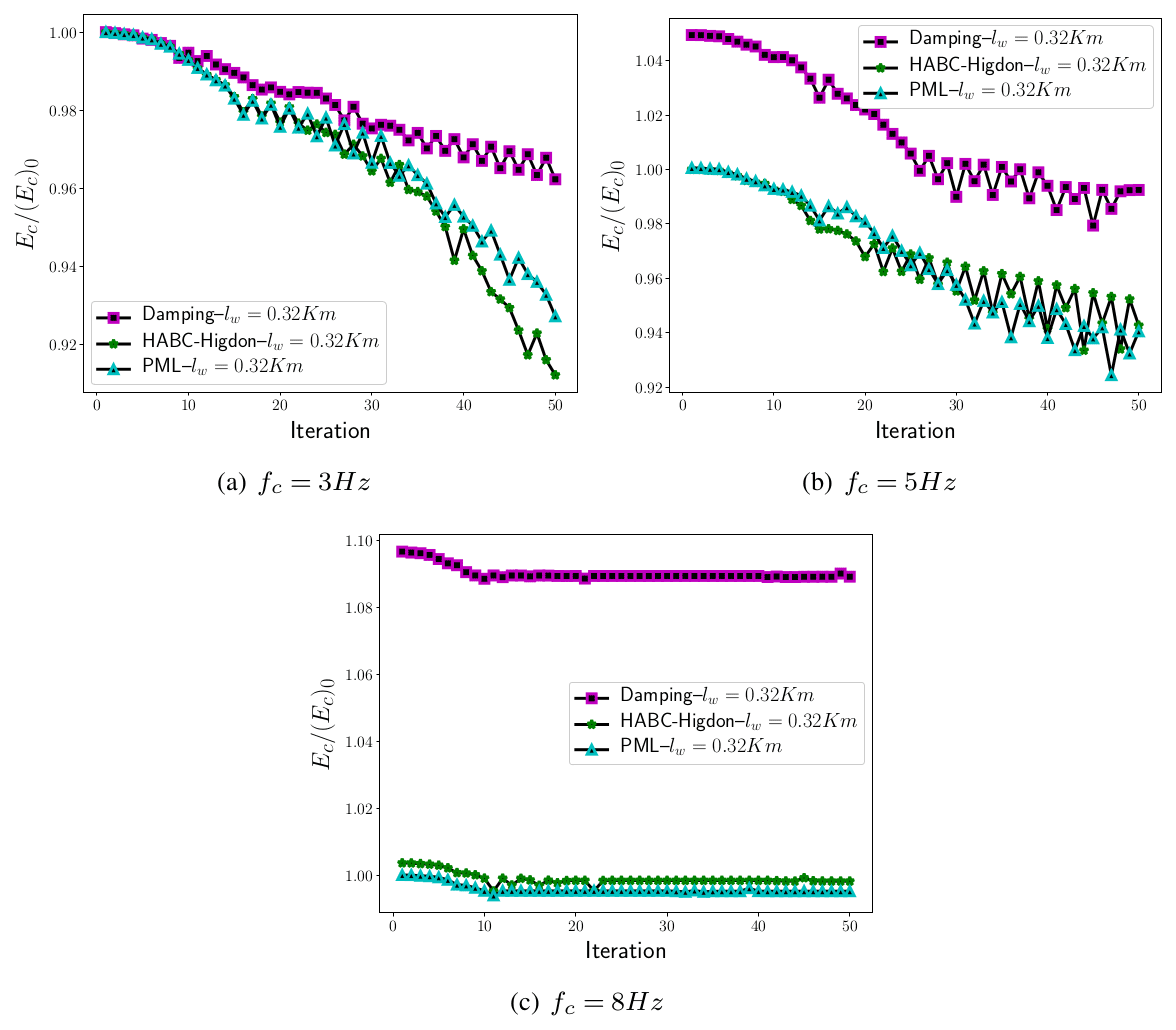
Figure 18Comparisons of the misfit values for velocity model computation that is then matched with Marmousi, where the peak of frequency is f0=15 Hz, and a multiscale approach in frequency (Bunks et al., 1995) is employed. (Ec)0 is computed at the first iteration, which is the minimal velocity error given by the employment of the damping, HABC-Higdon, and PML methods.
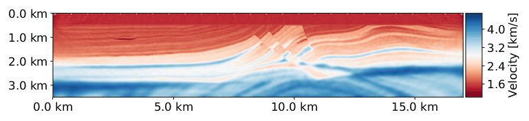
Figure 19Velocity model computed by the FWI execution with HABC-Higdon and a multiscale approach (Bunks et al., 1995).
Table 5The percent growth of wall clock time and RAM usage, as compared to the no-ABC case (lw=0.0 km). The measures are related to a source of a single shot wave of the FWI execution, with a multiscale approach, for the velocity model that is matched with Marmousi. It this case, the execution of FWI with no-ABC required 75 s of wall clock time and 6.11GB of memory usage.
This work evaluates the effectiveness of the ABC methods in mitigating spurious boundary reflections, by employing a setting that is usually adopted in FWI applications. The analyses were carried out for the forward and adjoint wave equations, and our findings clearly show that the adjoint problem also experiences spurious boundary reflections. Indeed, that should be expected, owing to the hyperbolic character that those equations share with their physical counterparts. In view of such evidence, we have formally derived adjoint boundary conditions that correspond to each of the ABCs. This formulation of forward and adjoint problems, along with their corresponding ABCs, has been extensively tested to assess the effectiveness of the latter. A number of application cases has been run for heterogeneous velocity models, ranging from the simplest models to realistic ones.
Code development was carried out in the domain-specific language (DSL) computational framework, Devito, which allows an easy implementation of the absorbing conditions described here. Furthermore, these schemes are readily available in the Devito repository (see the Devito tutorials on ABCs) to be used in more realistic problems, and they may be adapted to three-dimensional problems by means of symbolic operations alone.
Analyses of the ABCs' effectiveness in the forward and adjoint problems have shown that the PML and HABC-Higdon are more effective for both of them. On the other hand, the damping method is the least efficient method for attenuating reflections. Figures 17 and 18 depict it as being less effective than the HABC-Higdon, even when an effort is made to improve matters by increasing the size of the domain extension. The CPML method has presented higher errors than the PML and HABC-Higdon, and it has not kept a pattern, with different levels of effectiveness for the forward and adjoint problems. For instance, Fig. 9 shows smaller errors for the CPML than for the HABC-A1 and damping methods. Yet, for the adjoint problem, Fig. 12a shows CPML errors to be higher than those of the damping method as the peak of frequency f increases.
On evaluating the computational cost of ABCs methods, HABC-Higdon has shown the best performance, since its errors are either close to or smaller than those of the PML in several cases, and its computational cost is lower than the PML or damping with larger extensions. A similar conclusion may be drawn for the FWI applications, where the HABC-Higdon has shown to require less memory usage and wall clock time than the FWI with PML method. On accounting for the computational cost and effectiveness, the tests have indicated that the HABC-Higdon also performs better than the damping method. To be more specific, Table 4 shows the percent of growth of memory usage and wall clock time of the damping method to be higher than those of HABC-Higdon when the extended domain was increased from lw=0.67 to 2.5 km. In such a case, the HABC-Higdon with lw=0.67 km was more effective in mitigating reflections than the damping method with lw=2.5.
Regarding the extension to 3D problems, previous works (Grote and Sim, 2010; Xie et al., 2014) on PML methods did not report on differences in attenuation effectiveness when going from 2D to 3D domains. Owing to the symmetric nature of the acoustic wave propagation, we also expect the effectiveness of the ABCs in 3D problems to be similar to those shown here. The computational cost, however, may be considerably different, which should, in principle, raise the differences between them. The computational costs in the 3D applications may be estimated by using data from Tables 4 and 5. For instance, take the computational cost from Table 5 as a basis, with the third additional dimension, the y direction of length of ly, which is discretized for finite differences for a grid spacing of Δy. In this case, the growth of computational costs of an FWI application (and memory usage) become at least times larger than those of the 2D using the no-ABC case, damping, and HABC-Higdon. However, with the damping scheme requiring a larger extension region, the memory savings of the HABC-Higdon in 3D problems become even more evident than in the 2D. With both damping and HABC-Hybrid schemes, no additional variables or equations are required when going from 2 to 3 dimensions, whereas the PML does entail two additional PDEs in that case. This makes the rise in computational costs of the PML even higher when one adds the third dimension, when compared to the corresponding cases of the no-ABC or the HABC-Higdon, as can be seen in Tables 4 and 5.
While this work has adopted synthetic velocity models to generate the true seismogram data in the FWI problems, our findings regarding the ABCs are expected to hold just as well for real seismograms, since the spurious reflections arise on the computational solver where artificial outer boundaries are imposed. Hence, they are just as prone to exhibiting spurious reflections, as the above tests have shown. In addition, the velocity model represents a medium where the wave propagates. Thus, the velocity field affects the angle of incidence at which the wave reaches the truncated boundaries. The ABCs have a good performance when the incidence angle is closer to the normal direction than to the truncated boundary but lose their effectiveness at glancing angles of incidence, i.e. closer to 90∘ (Gao et al., 2017). In principle, then, any particular model poses its own set of challenges to those techniques. Here, we consider widely used models, such as the SEG/EAGE and Marmousi models, as examples of realistic models (Chi et al., 2014; Sun and Demanet, 2020; Zhu et al., 2022; Buchatsky and Treister, 2021).
Since the ABC formulations presented here are available for general wave equations (e.g. elastic/viscous acoustic), the methods can be applied for different physics problems of wave propagation. Komatitsch and Tromp (2003) verified that PML condition is efficient for both pressure (P) and shear (S) waves. In an anisotropic medium, Dimitri (2007) showed that the CPML methods were efficient at absorbing the quasi-pressure wave and the quasi-shear wave. The HABC-A1 and HABC-Higdon are based on Clayton's A1 and Higdon conditions, respectively. Engquist and Majda (1977) and Higdon (1991) evaluated the effectiveness of the ABCs methods for P and S waves. So, while not shown here, the ABCs presented in this work should be able to attenuate the spurious reflections generated in the truncated boundaries for other physics problems. Furthermore, previous works (Gao et al., 2017; Engquist and Majda, 1977; Higdon, 1991) indicated that the angle of incidence at which the waves reach the truncated boundaries has more of an effect on the ABCs' performance than the wave propagation properties. Therefore, we expect that, overall, our results should hold for different physics, as long as they still rely on wave propagation physics.
This Appendix presents the formulation of the adjoint equations for each ABC method. To do so, the augmented functional is considered, in which the constraints are given by the wave equation and by the equations used in ABCs.
As shown before, to apply any of the ABCs of interest in this study, the domain considered is built as the union of the physical domain Ω0 and the extended domain . In FWI, the goal is to minimize the objective functional I(m) on the physical domain Ω0. Therefore, the objective functional remains by being defined by the expression (1) but is now defined over Ω0.
A1 Damping
The acoustic wave equation with damping mechanism is given by Eq. (6). The corresponding adjoint equations are obtained by pursuing the same sequence presented by Plessix (2006). So, the first step is to write the augmented functional value, considering the equations defined in the physical and in the extended domains, as follows:
where and ζ=ζ(x).
In the current case, the wave equation with damping mechanism is defined in the domain Ω illustrated by the blue region in Fig. 1b. To obtain the adjoint equation, their initial and boundary conditions, the gradient , are written as follows:
where u′ is a perturbation of the variable u.
Integration by parts is applied, as shown below, in the following:
where the gradient ∇u[I(m)]u′ is given by the following:
The term ℬ is the bilinear concomitant, which entails the integration by parts. After applying the divergence theorem, ℬ reads as follows:
The adjoint wave equation and their initial and boundary conditions are then defined by imposing . That means defining the adjoint equation as follows:
Also, on considering the boundary and initial conditions of the forward wave equation and by imposing the adjoint boundary conditions, which are given by the following:
The bilinear concomitant is reduced to the following:
The homogeneous initial conditions of the forward wave equation drive the domain integral to zero, which is evaluated at t0=0. In order to eliminate the corresponding domain integral for t=tf, one could impose the following homogeneous final conditions on the adjoint variable, as follows, where u†:
To make the algebra simpler with respect to these conditions, one could define an adjoint time variable in the following form:
As a result of this change in variables, the adjoint wave equation (Eq. A2) becomes the following in its final form:
which means it is a self-adjointing wave equation.
A2 PML and CPML
The work of Xie et al. (2014) presents a mathematical development to obtain the adjoint wave system with the referred complex-frequency-shifted unsplit-field perfectly matched layer (CFS-UPML). In essence, the Fourier transform of the displacement vector, u, satisfies the Helmholtz equation as follows:
where s∈𝒞. Also, one considers the transformation of the following spatial coordinates, x, as follows:
Here, for the 2D case, is the complex stretching function, as follows:
and .
The next step consists of reformulating Eq. (A7) in the time domain. In the 2D case, it leads to the following:
where , ℱ−1 is the inverse Fourier transform, and ∗ represents a convolution.
On taking the wave equation (Eq. A8) into account, the adjoint system is then defined as follows (Xie et al., 2014):
which satisfies the conditions in Eqs. (A3), (A4), and (A5).
In the standard PML formulation, αj=0, κj=1 (Berenger, 1994). Therefore, the adjoint wave equation with PML is a particular case of the methodology presented by Xie et al. (2014). Hence, for the 2D case, the convolutions of the adjoint wave in Eq. (A9) are given by the following:
where H(t) is the Heaviside distributions.
The convolution terms and may be solved by considering auxiliary differential equations (Grote and Sim, 2010; Xie et al., 2014). On defining the auxiliary functions, as follows:
Thus, the terms in Eqs. (A11) and (A12) are rewritten as follows:
Therefore, the adjoint wave Eq. (A9) with the employment of PML method reads as follows:
where the auxiliary functions and satisfy the respective auxiliary differential equations, as follows:
The adjoint wave in Eq. (A9) may be also written according to the formulation presented in Pasalic and McGarry (2010), i.e. the CPML formulation. In this case, αj is a positive value, and κj=1 (Pasalic and McGarry, 2010). Therefore, to write an adjoint system with CPML method, Eq. (A9) is rewritten as follows:
where . Using Pasalic and McGarry (2010), we have the following:
Therefore, the adjoint wave in Eq. (A16) is cast in the following form:
where the auxiliary functions (, , , ) are obtained by using the auxiliary equations given by the following:
A3 Hybrid absorbing boundary condition (HABC)
The HABC methods apply the discrete convex combination (Eq. 26) to a discrete transitional area of Ωe. As explained in Sect. 3.5, this approach combines the solution of the wave equation with the boundary conditions of Clayton’s A1 condition for HABC-A1 and Higdon for HABC-Higdon. So, to derive the adjoint equations, let us start by considering boundary conditions on the truncated boundaries (, ) that satisfy the Clayton's A1. In this case, the augmented functional is given by Eq. (3).
On integrating it by parts, one arrives at the following:
where the adjoint wave equation is defined by Eq. (5), reaching . On adopting the boundary condition at the free surface (Eq. A4), and zero initial conditions of the forward and adjoint variables, it yields the following:
In the truncated boundaries, , Clayton's A1 boundary condition reads as follows:
which implies Hence, the right-hand side term of Eq. (A22) is rewritten as follows:
Next, the integration by parts with respect to time can be applied, and Eq. (A22) becomes the following:
since is satisfied. Last, on imposing , the extremum is then realized.
The same approach may be employed to obtain the adjoint wave equation in the case where the Higdon boundary condition is imposed on the truncated boundaries . Therefore, the adjoint wave equation is defined by Eq. (5). Also, on imposing the boundary condition at the free surface (Eq. A4) and zero initial conditions for the forward (u) and adjoint (u†) variables, the gradient is reduced to Eq. (A22). So, based on Higdon (1986), Higdon's boundary condition was proposed by considering the wave propagating outward at an angle of incidence, α. In a two-dimensional domain, the wave solution was described by . Hence, the generalized boundary condition is as follows:
such that for all j. That allows us to write , and Eq. (A22) is as follows:
On integrating it by parts in time, the above equation becomes the following:
As a result of it, on imposing , the extreme is attained, and the generalization is as follows:
which may be imposed as boundary conditions on the adjoint wave problem.
The reproducible code can be founded in the following Zenodo directory: https://doi.org/10.5281/zenodo.6003038 (Dolci et al., 2022).
The velocity data sets used in this work were created synthetically (circle) or obtained in a open data set repository (Marmousi, Martin et al., 2006, and 2D/SEG EAGE, Aminzadeh and Brac, 1997; https://wiki.seg.org/wiki/Open_data, last access: 15 September 2021).
DID and FAGS took responsibility for the conceptualization, methodology, and software and prepared the original draft. DID led the investigation, and FAGS did the validation. PSP and EVV supervised, reviewed, and edited the paper and acquired the resources and funding.
The contact author has declared that none of the authors has any competing interests.
Publisher's note: Copernicus Publications remains neutral with regard to jurisdictional claims in published maps and institutional affiliations.
This research was carried out in association with the ongoing R& D project, registered as ANP 20714-2 STMI – Software Technologies for Modelling and Inversion, with applications in seismic imaging (USP/Shell Brasil/ANP).
The authors would also like to acknowledge and express their deepest appreciation for the invaluable contribution that the late Saulo R. M. de Barros (1958–2021) made to this work. He has done so much for our research. Sadly, though, he did not live to see it bear fruit.
This research has been supported by the Agência Nacional do Petróleo, Gás Natural e Biocombustíveis (ANP grant no. 20714-2).
This paper was edited by Thomas Poulet and reviewed by two anonymous referees.
Abubakar, A., Hu, W., Habashy, T. M., and Van den Berg, P.: Application of the finite-difference contrast-source inversion algorithm to seismic full-waveform data, Geophysics, 74, WCC47–WCC58, https://doi.org/10.1190/1.3250203, 2009. a, b
Aghamiry, H. S., Gholami, A., and Operto, S.: Improving full-waveform inversion by wavefield reconstruction with the alternating direction method of multipliers, Geophysics, 84, R139–R162, https://doi.org/10.1190/geo2018-0093.1, 2019. a, b
Aminzadeh, F., Brac, J., and Kunz, T.: SEG/EAGE 3-D Salt and Overthrust Models, 1, Distribution CD of Salt and Overthrust models, SEG book series [data set], https://wiki.seg.org/wiki/SEG/EAGE_Salt_and_Overthrust_Models (last access: 26 June 2022), 1997. a, b, c
Asnaashari, A., Brossier, R., Garambois, S., Audebert, F., Thore, P., and Virieux, J.: Regularized seismic full waveform inversion with prior model information, Geophysics, 78, R25–R36, https://doi.org/10.1190/geo2012-0104.1, 2012. a, b
Ben-Hadj-Ali, S., Operto, S., and Virieux, J.: An efficient frequency-domain full waveform inversion method using simultaneous encoded sources, Geophysics, 76, R109–R124, https://doi.org/10.1190/1.3581357, 2011. a, b
Berenger, J.-P.: A perfectly matched layer for the absorption of electromagnetic waves, J. Comput. Phys., 114, 185–200, https://doi.org/10.1006/jcph.1994.1159, 1994. a
Buchatsky, S. and Treister, E.: Full waveform inversion using extended and simultaneous sources, SIAM J. Sci. Comp., 43, S862–S883, https://doi.org/10.1137/20M1349412, 2021. a
Bunks, C., Saleck, F. M., Zaleski, S., and Chavent, G.: Multiscale seismic waveform inversion, Geophysics, 60, 1457–1473, https://doi.org/10.1190/1.1443880, 1995. a, b, c, d
Byrd, R. H., Lu, P., Nocedal, J., and Zhu, C.: A limited memory algorithm for bound constrained optimization, SIAM J. Sci. Stat. Comp., 16, 1190–1208, https://doi.org/10.1137/0916069, 1995. a
Chi, B., Dong, L., and Liu, Y.: Full waveform inversion method using envelope objective function without low frequency data, J. Appl. Geophys., 109, 36–46, https://doi.org/10.1016/j.jappgeo.2014.07.010, 2014. a
Clayton, R. and Engquist, B.: Absorbing boundary conditions for acoustic and elastic wave equations, B. Seismol. Soc. Am., 67, 1529–1540, https://doi.org/10.1785/BSSA0670061529, 1977. a, b
Dimitri, K.: An unsplit convolutional perfectly matched layer improved at grazing incidence for the seismic wave equation, Geophysics, 72, 255–167, https://doi.org/10.1190/1.2757586, 2007. a
Dolci, D. I., Silva, F. A. G., Peixoto, P. S., and Volpe, E. V.: felipeaugustogudes/paper-fwi: v1.0 (v1.0), Zenodo [code], https://doi.org/10.5281/zenodo.6003038, 2022. a
Engquist, B. and Majda, A.: Absorbing boundary conditions for numerical simulation of waves, P. Natl. Acad. Sci. USA, 74, 1765–1766, https://doi.org/10.1073/pnas.74.5.1765, 1977. a, b
Fichtner, A., H.-P. Bunge, H. I.: The adjoint method in seismology: I. Theory, Phys. Earth Planet. Int., 157, 86–104, https://doi.org/10.1016/j.pepi.2006.03.016, 2006. a, b, c
Fichtner, A.: Full seismic waveform modelling and inversion, Springer Science & Business Media, 2010. a
Fornberg, B.: Generation of finite difference formulas on arbitrarily spaced grids, Math. Comp., 51, 699–706, 1988. a
Gao, Y., Song, H., Zhang, J., and Yao, Z.: Comparison of artificial absorbing boundaries for acoustic wave equation modelling, Explor. Geophys., 48, 76–93, https://doi.org/10.1071/EG15068, 2017. a, b, c, d, e, f, g, h
Grote, M. J. and Sim, S.: Efficient pml for the wave equation, arXiv preprint arXiv, https://doi.org/10.48550/arXiv.1001.0319, 2010. a, b, c, d, e, f, g
Higdon, R. L.: Absorbing boundary conditions for difference approximations to the multidimensional wave equation, Math. Comp., 47, 437–459, https://doi.org/10.2307/2008166, 1986. a, b, c, d
Higdon, R. L.: Numerical absorbing boundary conditions for the wave equation, Math. Comp., 49, 65–90, https://doi.org/10.1090/S0025-5718-1987-0890254-1, 1987. a, b, c
Higdon, R. L.: Absorbing boundary conditions for elastic waves, Geophysics, 56, 231–241, https://doi.org/10.1190/1.1443035, 1991. a, b
Kaltenbacher, B., Kaltenbacher, B., and Sim, I.: A modified and stable version of a perfectly matched layer technique for the 3-d second order wave equation in time domain with an application to aeroacoustics, J. Comput. Phys., 235, 407–422, https://doi.org/10.1016/j.jcp.2012.10.016, 2013. a
Komatitsch, D. and Tromp, J.: A perfectly matched layer absorbing boundary condition for the second-order seismic wave equation, Geophys. J. Int., 154, 146–153, https://doi.org/10.1046/j.1365-246X.2003.01950.x, 2003. a
Kukreja, N., Louboutin, M., Vieira, F., Luporini, F., Lange, M., and Gorman, G.: Devito: Automated fast finite difference computation, in: 2016 Sixth International Workshop on Domain-Specific Languages and High-Level Frameworks for High Performance Computing (WOLFHPC), IEEE, 11–19, https://doi.org/10.1109/WOLFHPC.2016.06, 2016. a
Liu, Y. and Sen, M. K.: A hybrid scheme for absorbing edge reflections in numerical modeling of wave propagation, Geophysics, 75, A1–A6, https://doi.org/10.1190/1.3295447, 2010. a, b, c
Liu, Y. and Sen, M. K.: A hybrid absorbing boundary condition for elastic staggered-grid modelling, Geophys. Pros., 60, 1114–1132, https://doi.org/10.1111/j.1365-2478.2011.01051.x, 2012. a, b, c
Liu, Y. and Sen, M. K.: An improved hybrid absorbing boundary condition for wave equation modeling, J. Geophys. Eng., 15, 2602–2613, https://doi.org/10.1088/1742-2140/aadd31, 2018. a, b, c, d, e
Louboutin, M., Lange, M., Luporini, F., Kukreja, N., Witte, P. A., Herrmann, F. J., Velesko, P., and Gorman, G. J.: Devito (v3.1.0): an embedded domain-specific language for finite differences and geophysical exploration, Geosci. Model Dev., 12, 1165–1187, https://doi.org/10.5194/gmd-12-1165-2019, 2019. a, b, c
Luporini, F., Lange, M., Louboutin, M., Kukreja, N., Hückelheim, J., Yount, C., Witte, P., Kelly, P. H. J., Herrmann, F. J., and Gorman, G. J.: Architecture and performance of Devito, a system for automated stencil computation, CoRR, abs/1807.03032, http://arxiv.org/abs/1807.03032 (last access: 7 February 2020), 2018. a, b
Martin, G. S., Wileya, R., and Kurt, J.: Marmousi2 : An elastic upgrade for Marmousi, The Leading Edge, 25, 156–166, https://doi.org/10.1190/1.2172306, 2006. a, b, c
Mora, P.: Nonlinear two-dimensional elastic inversion of multioffset seismic data, Geophysics, 52, 1211, https://doi.org/10.1190/1.1442384, 1987. a, b
Pasalic, D. and McGarry, R.: Convolutional perfectly matched layer for isotropic and anisotropic acoustic wave equations, in: SEG Technical Program Expanded Abstracts 2010, Society of Exploration Geophysicists, 2925–2929, https://doi.org/10.1190/1.3513453, 2010. a, b, c, d, e
Plessix, R.-E.: A review of the adjoint-state method for computing the gradient of a functional with geophysical applications, Geophys. J. Int, 167, 495–503, https://doi.org/10.1111/j.1365-246X.2006.02978.x, 2006. a, b, c
Ricker, N.: The form and nature of seismic waves and the structure of seismograms, Geophysics, 5, 348–366, https://doi.org/10.1190/1.1441816, 1940. a
Sochacki, J., Kubichek, R., George, J., Fletcher, W., and Smithson, S.: Absorbing boundary conditions and surface waves, Geophysics, 52, 60–71, https://doi.org/10.1190/1.1442241, 1987. a, b, c, d
Sun, H. and Demanet, L.: Extrapolated full-waveform inversion with deep learningEFWI-CNN, Geophysics, 85, R275–R288, https://doi.org/10.1190/geo2019-0195.1, 2020. a
Tarantola, A.: Inversion of seismic reflection data in the acoustic approximation, Geophysics, 49, 1259–1266, https://doi.org/10.1190/1.1441754, 1984. a, b, c, d
Tarantola, A.: A strategy for nonlinear elastic inversion of seismic reflection data, Geophysics, 51, 1893–1903, https://doi.org/10.1190/1.1442046, 1986. a
Tarantola, A.: Theoretical background for the inversion of seismic waveforms including elasticity and attenuation, Pure Appl. Geophys., 128, 365–399, https://doi.org/10.1007/BF01772605, 1988. a
Virieux, J. and Operto, S.: An overview of full-waveform inversion in exploration geophysics, Geophysics, 74, WCC1–WCC26, https://doi.org/10.1190/1.3238367, 2009. a, b
Xie, Z., Komatitsch, D., Martin, R., and Matzen, R.: Improved forward wave propagation and adjoint-based sensitivity kernel calculations using a numerically stable finite-element PML, Geophys. J. Int., 198, 1714–1747, https://doi.org/10.1093/gji/ggu219, 2014. a, b, c, d, e
Zhu, W., Xu, K., Darve, E., Biondi, B., and Beroza, G. C.: Integrating deep neural networks with full-waveform inversion: Reparameterization, regularization, and uncertainty quantification, Geophysics, 87, R93–R109, https://doi.org/10.1190/geo2020-0933.1, 2022. a
- Abstract
- Introduction
- The FWI problem
- ABCs in forward problem
- ABCs in adjoint problem
- Computational framework
- Analysis of ABCs
- Analysis of ABCs in a FWI problem
- Conclusions
- Appendix A: Formulation of the adjoint equations
- Code availability
- Data availability
- Author contributions
- Competing interests
- Disclaimer
- Acknowledgements
- Financial support
- Review statement
- References