the Creative Commons Attribution 4.0 License.
the Creative Commons Attribution 4.0 License.
 | 27 Jul 2022
Cloud-based framework for inter-comparing submesoscale-permitting realistic ocean models
Takaya Uchida
Julien Le Sommer
Charles Stern
Ryan P. Abernathey
Chris Holdgraf
Aurélie Albert
Laurent Brodeau
Eric P. Chassignet
Xiaobiao Xu
Jonathan Gula
Guillaume Roullet
Nikolay Koldunov
Sergey Danilov
Qiang Wang
Dimitris Menemenlis
Clément Bricaud
Brian K. Arbic
Jay F. Shriver
Fangli Qiao
Bin Xiao
Arne Biastoch
René Schubert
Baylor Fox-Kemper
William K. Dewar
Alan Wallcraft
With the increase in computational power, ocean models with kilometer-scale resolution have emerged over the last decade. These models have been used for quantifying the energetic exchanges between spatial scales, informing the design of eddy parametrizations, and preparing observing networks. The increase in resolution, however, has drastically increased the size of model outputs, making it difficult to transfer and analyze the data. It remains, nonetheless, of primary importance to assess more systematically the realism of these models. Here, we showcase a cloud-based analysis framework proposed by the Pangeo project that aims to tackle such distribution and analysis challenges. We analyze the output of eight submesoscale-permitting simulations, all on the cloud, for a crossover region of the upcoming Surface Water and Ocean Topography (SWOT) altimeter mission near the Gulf Stream separation. The cloud-based analysis framework (i) minimizes the cost of duplicating and storing ghost copies of data and (ii) allows for seamless sharing of analysis results amongst collaborators. We describe the framework and provide example analyses (e.g., sea-surface height variability, submesoscale vertical buoyancy fluxes, and comparison to predictions from the mixed-layer instability parametrization). Basin- to global-scale, submesoscale-permitting models are still at their early stage of development; their cost and carbon footprints are also rather large. It would, therefore, benefit the community to document the different model configurations for future best practices. We also argue that an emphasis on data analysis strategies would be crucial for improving the models themselves.
- Article
(20890 KB) - Full-text XML
- BibTeX
- EndNote


Traditionally, collaboration amongst multiple ocean modeling institutions and/or the reproduction of scientific results from numerical simulations required the duplication, individual sharing, and downloading of data, upon which each of the interested parties (or an independent group) would analyze the data on their local workstation or cluster. We will refer to this as the “download” framework (Stern et al., 2022a). As realistic ocean simulations with kilometric horizontal resolution have emerged (e.g., Rocha et al., 2016; Schubert et al., 2019; Brodeau et al., 2020; Gula et al., 2021; Ajayi et al., 2021), such a framework has become cumbersome, with terabytes and petabytes of data needed to be transferred and stored as ghost copies. Nevertheless, a real demand exists for collaboration to inter-compare models to examine their fidelity and quantify robust features of submesoscale and mesoscale turbulence (the former on the horizontal spatial scales of O(10 km) and the latter on O(100 km), from here on referred to jointly as (sub)mesoscale; Hallberg, 2013; McWilliams, 2016; Lévy et al., 2018; Uchida et al., 2019; Dong et al., 2020). The Ocean Model Intercomparison Project (OMIP), for example, has been successful in diagnosing systematic biases in non-eddying and mesoscale-permitting ocean models used for global climate simulations (Griffies et al., 2016; Chassignet et al., 2020).
Here, we would like to achieve the same goal as OMIP but by inter-comparing submesoscale-permitting ocean models, which have been argued to be sensitive to grid-scale processes and numerical schemes as we increasingly push the model resolution closer to the scales of non-hydrostatic dynamics and isotropic three-dimensional (3D) turbulence (Hamlington et al., 2014; Soufflet et al., 2016; Ducousso et al., 2017; Barham et al., 2018; Bodner and Fox-Kemper, 2020). Considering the enormous computational cost and carbon emission of these submesoscale-permitting models, it would also benefit the ocean and climate modeling community to compile the practices implemented by each modeling group for future runs. In doing so, we analyze eight realistic, submesoscale-permitting ocean simulations, which cover at least the North Atlantic basin, run with the code bases of the Nucleus for European Modelling of the Ocean (NEMO; Madec et al., 2019, https://www.nemo-ocean.eu/, last access: 8 July 2022), Coastal and Regional Ocean COmmunity model (CROCO; Shchepetkin and McWilliams, 2005, https://www.croco-ocean.org/, last access: 8 July 2022), Massachusetts Institute of Technology general circulation model (MITgcm; Marshall et al., 1997, https://mitgcm.readthedocs.io/en/latest/, last access: 8 July 2022), HYbrid Coordinate Ocean Model (HYCOM; Bleck, 2002; Chassignet et al., 2009, https://www.hycom.org/, last access: 8 July 2022), Finite volumE Sea ice-Ocean Model (FESOM; Danilov et al., 2017, https://fesom2.readthedocs.io/en/latest/index.html, last access: 8 July 2022), and First Institute of Oceanography Coupled Ocean Model (FIO-COM, http://fiocom.fio.org.cn/, last access: 8 July 2022). Considering the amount of data, however, the download framework becomes very inefficient. Therefore, we have implemented the “data-proximate computing” framework proposed by the Pangeo project where we have stored the model outputs on the cloud and brought the computational resources adjacent to the data on the cloud (Abernathey et al., 2021a; Stern et al., 2022a).
Many of these simulations were developed ahead of the Surface Water and Ocean Topography (SWOT) satellite launch (Morrow et al., 2019), now projected to be in November 2022, in order to allow for the instrumental calibration of SWOT (Gomez-Navarro et al., 2018; Metref et al., 2020) and to disentangle the internal wave signals from (sub)mesoscale flows; SWOT is expected to observe the superposed field of the two dynamics (Savage et al., 2017a; Torres et al., 2018; Yu et al., 2021). During its calibration phase, SWOT will pass over the same site every day for 6 months and have tracks that will cross over with each other. In order to showcase the data-proximate computing framework and its potential for collaborative, open-source, and reproducible science, we provide example diagnostics for one of the SWOT Crossover (Xover) regions around the Gulf Stream separation (Region 1 in Fig. 1). We leave the detailed diagnostics of (sub)mesoscale flows including other SWOT Xover regions and the potential impact of modeling numerics on the resolved flow for a subsequent paper.
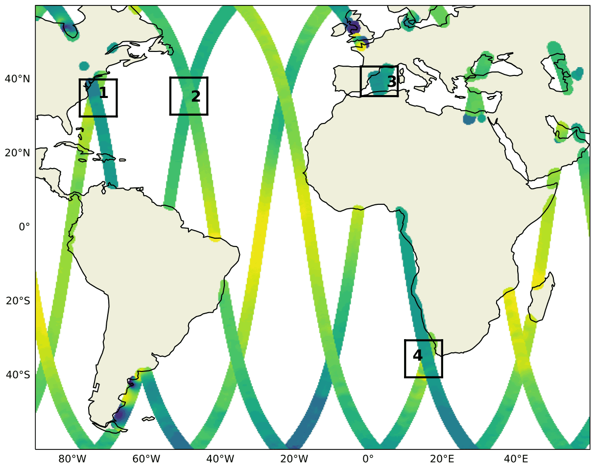
Figure 1SWOT tracks during its calibration phase and strategic Xover regions in the Atlantic sector. The regions cover the Gulf Stream separation and its extension (Regions 1 and 2), the western Mediterranean Sea (Region 3), and the Agulhas Rings (Region 4).
The paper is organized as follows. We describe the data-proximate computing framework in Sect. 2 and showcase some example analyses using this framework in Sect. 3. Cautionary remarks regarding sustainability into the future for open-source reproducible science are given in Sect. 4, and we conclude in Sect. 5.
In order for the data-proximate computing framework to work for collaborative, open-source, and reproducible science, it requires two components to work together simultaneously: (i) public access to analysis-ready data and (ii) open-source computational resources adjacent to the data.
2.1 Analysis-ready cloud-optimized data
In the field of Earth science, model outputs are often archived and distributed in binary, HDF5, or NetCDF formats. While we have greatly benefitted from these formats, they are not optimized for cloud storage or for parallelized cloud computing. However, as Earth scientists, commonly, we do not possess the training in cloud infrastructure or the data engineering required to efficiently convert large-scale archival datasets into formats which allow us to leverage the full performance potential of the commercial cloud. Data engineers, on the other hand, do not know the scientific needs of the data. In collaboration with Pangeo Forge (Stern et al., 2022a, https://pangeo-forge.readthedocs.io/en/latest/, last access: 8 July 2022), we have therefore attempted to fill this niche by streamlining the process of data preparation and submission. To transform their data into analysis-ready cloud-optimized (ARCO) formats, data providers (ocean modeling institutions in our case) need only specify the source file location (e.g., as paths on an ftp, http, or OPeNDAP server) along with output dataset parameters (e.g., particular ARCO format, chunking) in a Python module known as a recipe. The recipe module, which is typically a few dozen lines of Python code, relies on a data model defined in the open-source pangeo-forge-recipes package. Once complete, the recipe is submitted via a pull request on Github to the Pangeo Forge staged-recipes repository (https://github.com/pangeo-forge/staged-recipes, last access: 8 July 2022).
From here, Pangeo Forge automates the process of converting the data into ARCO format and storing the resulting dataset on the cloud, using its own elastically scaled cloud compute cluster. The term “analysis-ready” here is used broadly to refer to any dataset that has been preprocessed to facilitate the analysis which will be performed on it (Stern et al., 2022a).
An example of such a recipe for eNATL60 described in Sect. 3 is given in Appendix A. We refer the interested reader to Abernathey et al. (2021a) and Stern et al. (2022a) for further details on the technical implementation.
The crowd-sourcing approach of Pangeo Forge, to which any data provider can contribute, not only benefits the immediate scientific needs of a single research project, but also the entire scientific community in the form of shared, publicly accessible ARCO datasets which remain available for all to access. This saves each scientist the cost of duplicating and storing ghost copies of the data and allows for reproducible science. The model outputs used for this study are stored on the Open Storage Network (OSN), a cloud storage service provided by the National Science Foundation (NSF) in the US. The surface data were saved hourly and interior data in the upper 1000 m as daily averages (due to cloud storage constraints).
To facilitate the access of data from OSN, we have further made them readable via intake, a data access and cataloging system which unifies the application programming interface (API) to read and load the data (https://intake.readthedocs.io/en/latest/overview.html, last access: 8 July 2022). That is, the API to read and load the data is the same for all of the data used in this project, regardless of its distribution format (e.g., binary, HDF5, or NetCDF), because each of the datasets has been converted by Pangeo Forge into the cloud-optimized Zarr format (https://zarr.readthedocs.io/en/stable/, last access: 8 July 2022) and subsequently cataloged with intake prior to analysis. This is particularly beneficial for our case, where we would like to systematically analyze multiple data collections.
The entire process of zarrifying the data, fluxing them to OSN, and cataloging scaled well for the four regions shown in Fig. 1; the net amount of data stored on OSN as of writing sums up to O(2 Tb).
While the amount of O(2 Tb) may seem small, the ARCO framework negates the generation and storage of ghost copies and scales as the data size increases. Jupyter notebooks for the results shown in Sect. 3, including the Yaml file to access data via intake, are given in the Pangeo Data swot_adac_ogcms Github repository (Stern et al., 2022b, https://github.com/pangeo-data/swot_adac_ogcms, last access: 8 July 2022).
Regarding LLC4320, the data were accessed via the Estimating the Circulation and Climate of the Ocean (ECCO) data portal. While there was no particular sub-setting applied to their dataset prior to analyses, the data portal and cloud-based JupyterHub being within geographical proximity (within the US) facilitated the data access. The combination of llcreader of the xmitgcm Python package to access their data in binary format (as opposed to NetCDF) also enhanced the efficiency (Abernathey, 2019; Abernathey et al., 2021b).
2.2 Cloud-based JupyterHub
For data-proximate computational resources, we have implemented JupyterHub, an open-source platform that provides remote access to interactive sessions in the cloud for many users (Fangohr et al., 2019; Beg et al., 2021), on the Google Cloud Platform (GCP). This infrastructure is run in collaboration with 2i2c.org, a non-profit organization based in the US that manages cloud infrastructure for open-source scientific workflows. Authentication for each user/collaborator on JupyterHub is provided via a white list of Github usernames, meaning that the hub can be accessed from anywhere and is not tied directly to an institutional account. This has allowed for real-time sharing of Python scripts amongst collaborators and exchange of feedback on the analytical results we present in Sect. 3. Cloud computing also offers the scaling of resources for improved I/O throughput and optimization of network bandwidth and central processing units (CPUs).
The model outputs used for this showcase are from the eNATL60 (Brodeau et al., 2020), GIGATL (Gula et al., 2021), HYCOM50 (Chassignet and Xu, 2017, 2021), FESOM-GS and LLC4320 (Rocha et al., 2016; Stewart et al., 2018), ORCA36 (https://github.com/immerse-project/ORCA36-demonstrator, last access: 8 July 2022), FIO-COM32 (Xiao et al., 2022), and HYCOM25 (Savage et al., 2017a, b; Arbic et al., 2018) simulations. The detailed configuration of each simulation is given in Appendix B. In order to motivate the reader on the necessity of inter-comparing realistic submesoscale-permitting simulations, we show in Fig. 2 the surface relative vorticity normalized by the local Coriolis parameter on 1 February at 00:00 GMT from each model. Despite their similar spatial resolutions, the spatial scales represented vary widely across models. Submesoscale-permitting ocean modeling is in its early stage of development, and each modeling institution is still exploring best practices. Therefore, we did not specify an experimental protocol, as in OMIP, for the model outputs from each institution. Each model uses different atmospheric products and tidal constituents to force the ocean, and the initial conditions and duration of spinup all vary (Appendix B). Nevertheless, we should expect statistical similarity in the oceanic flow at the spatial scales of O(10 km) if the numerics are robust.

Figure 2A snapshot of surface relative vorticity normalized by the local Coriolis parameter on 1 February at 00:00 from each model in Region 1.
3.1 Surface diagnostics of the temporal mean and variability
In light of the SWOT mission, the primary variable of interest is the ocean dynamic sea level. The AVISO estimate of this quantity is called the absolute dynamic topography (ADT), while the closely related model diagnostic is the sea surface height (SSH) after correcting for the inverse barometer effect if atmospheric pressure variability was simulated. Technically, SSH is defined as the geodetic height of the sea surface above the reference ellipsoid, while ocean dynamic sea level (or ADT) is defined relative to the geoid, but in models typically the geoid and reference ellipsoid coincide, so these two definitions are in practice the same (Gregory et al., 2019). Furthermore, in the specific comparisons made here, a regional average of the ocean dynamic sea level estimates is removed first, so that large-scale, slow changes (e.g., ice sheet mass loss contributions) are excluded from the comparison. From an ocean modeling perspective, one of the key features to argue in favor of increasing resolution in the North Atlantic has been the improvement in representing the Gulf Stream (GS) separation and the path of the North Atlantic Current (Chassignet and Xu, 2017; Chassignet et al., 2020; Chassignet and Xu, 2021). In assessing the models, it is common to examine the mean state, which we define as the time mean and variability about the mean. From the perspective of computational cost, the time mean of surface fields is the lightest, as the reduction in dimension allows for the download framework where the collaborators can share the averaged data. Variability about the time mean requires access to the temporal dimension, making the computational and data storage cost intermediate. We will further show in Sect. 3.2 an example of 3D diagnostics of the submesoscale flow, which significantly increases the computational cost and burden of transferring data; the 3D diagnostics will highlight the strength of the data-proximate framework where we can consistently apply the same diagnostic methods across different datasets.
In Fig. 3, we show the time mean and temporal standard deviation of ocean dynamic sea level from the eight models in the GS separation region. We also show the time mean ocean dynamic sea level estimated as ADT from the Archiving, Validation and Interpretation of Satellite Oceanographic (AVISO) data for reference. We do not show the standard deviation for AVISO as the spatiotemporal interpolation and smoothing limit its effective resolution to O(100 km) and O(10 d) (Chelton et al., 2011; Arbic et al., 2013; Chassignet and Xu, 2017). We provide the modeled standard deviations of ocean dynamic sea level filtered in a manner similar to the smoothing that goes into the AVISO products in Appendix C. The GS in most models tends to separate off of Cape Hatteras on the eastern coast of the US, consistent with AVISO (Fig. 3a, c, g, i, k, o, t). In terms of the magnitude of mean SSH, HYCOM50 may be overestimating it relative to AVISO across the path of the separated GS. The GS in LLC4320 tends to separate relatively southwards, while in FESOM-GS it separates northwards relative to AVISO observations, respectively (Fig. 3e and i). The separation in FESOM-GS may be closer to the observed state in 2014 (Fig. 3s) rather than 2012, the actual year of model output. Regarding the standard deviation, while expected, it is interesting that the simulations without tides (FESOM-GS and ORCA36; Fig. 3f and l) show significantly lower temporal variability compared to the other models. The low variability in FESOM-GS could also stem from the lack of atmospheric pressure variation in their atmospheric forcing (Table B6). Although HYCOM25 is tidally forced, its standard deviation is relatively low (Fig. 3p), which may be due to lower spatial resolution than the region- and basin-scale models used here (Table B2), the computational tradeoff of it being a global simulation. HYCOM25 nevertheless has higher values than FESOM-GS and ORCA36. The difference we find between simulations tidally forced and not is consistent with previous studies which argue that, in order to emulate the upcoming SWOT observations, applying tidal forcing is a key aspect in addition to model resolution (Savage et al., 2017a, b; Arbic et al., 2018; Torres et al., 2018; Ajayi et al., 2021; Yu et al., 2021). The benefit of having tidally forced simulations is that we can develop and test such methods of removing tides.
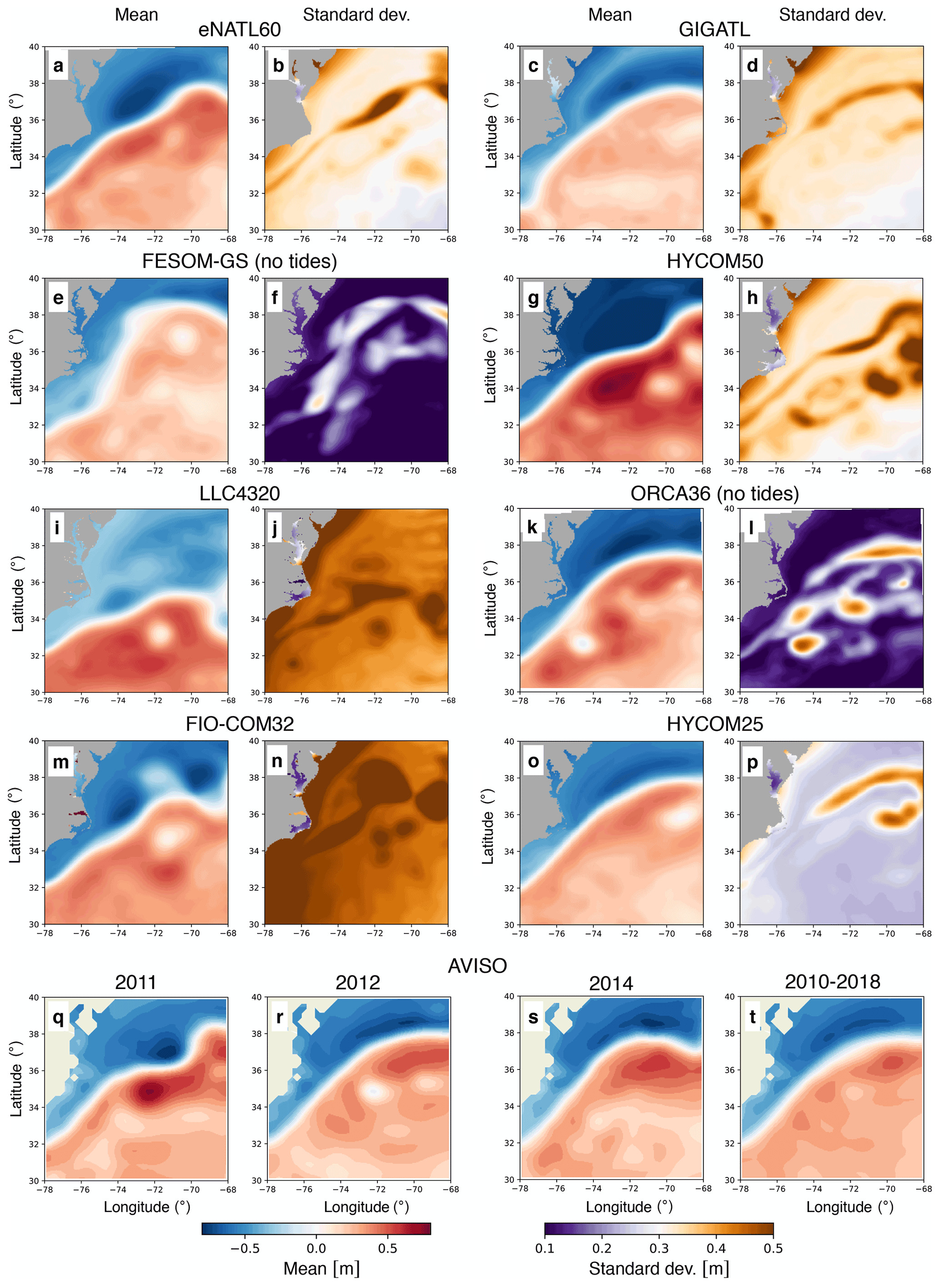
Figure 3The temporal mean and standard deviation of ocean dynamic sea level in the GS separation region (Region 1) during the months of February, March, and April using hourly outputs of SSH from the models. The bottom row shows the seasonal mean of ADT fields from AVISO during the months of February, March, and April. Daily AVISO data were used to compute the seasonal mean for three individual years (2011, 2012, and 2014) and over 2010–2018. The spatial mean is subtracted from the temporal mean fields from the models and AVISO to ensure that the mean SSH/ADT anomaly fields are comparable (i.e., large-scale contributions have been removed).
To complement the temporal standard deviation, in Fig. 4, we show the frequency spectra of SSH in the GS separation region. The frequency periodograms were computed every ∼10 km using the xrft Python package (Uchida et al., 2021) and then spatially averaged to compute the spectra. The temporal linear trend was removed, and a Hann window was applied prior to taking the Fourier transform of SSH as commonly done in studies examining spectra (e.g., Uchida et al., 2017; Savage et al., 2017a; Khatri et al., 2021). At frequencies higher than the Coriolis frequency, LLC4320 shows the highest variability and FESOM-GS the lowest for both winter and summer. FIO-COM32 shows the largest spectral amplitudes at the diurnal and semidiurnal frequencies amongst the models, which reflects itself in the large standard deviation (Fig. 3n). LLC4320 also shows the largest number of spectral peaks at tidal frequencies, likely due to being forced with full lunisolar tidal potential as opposed to a discrete number of tidal constituents, as was the case for the other models used here (Table B6). Also note that tidal forcing in the LLC4320 simulation was inadvertently overestimated by a factor of 1.1121. It is not surprising that FESOM-GS lacks spectral peaks at diurnal and semidiurnal frequencies, considering that it is not tidally forced. ORCA36, on the other hand, although not tidally forced, displays some activity at diurnal and semidiurnal frequencies, possibly due to the inclusion of atmospheric pressure variation in their forcing (Table B6). However, the lower peaks at tidal frequencies in ORCA36 compared to the tidally forced runs reflect themselves in the lower standard deviation as seen in Fig. 3l. eNATL60, GIGATL, HYCOM50, and HYCOM25 show similar levels of variability in the diurnal and semidiurnal bands. It is interesting to note that, at timescales of O(1–10 d), most runs show higher variability during winter than summer (Fig. 4a and c), while the tidally forced runs show higher variability at timescales shorter than O(1 d) during summer (Fig. 4b and d).
The seasonality at timescales shorter than O(1 d) is reversed for ORCA36, a run with no tidal forcing. It is possible that the increase in forward cascade of energy stimulated by the tides is the culprit in higher SSH variability at timescales shorter than the inertial frequency during summer than winter for the tidally forced runs and vice versa for the non-tidally forced runs (Barkan et al., 2021). The overall higher SSH variability at timescales longer than the inertial frequency during winter than summer, on the other hand, is possibly due to wind-driven inertial waves (Flexas et al., 2019).
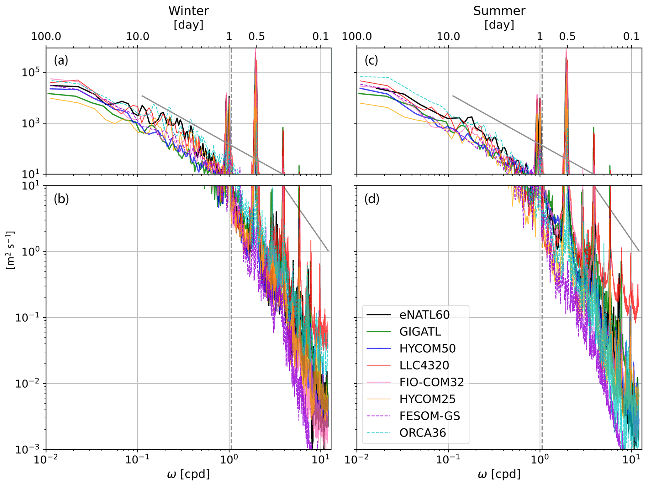
Figure 4The frequency spectra of hourly SSH for winter (February, March, April; a, b) and summer (August, September, October; c, d). The panels are split up at 10 m2 s−1 for visualization purposes. The frequency periodograms were computed every ∼10 km in Region 1 and then spatially averaged. The runs without tidal forcing (FESOM-GS and ORCA36) are shown in dashed lines. The Garrett–Munk spectral slope of ω−2 (Garrett and Munk, 1975) is shown as the grey solid line and the domain-averaged Coriolis frequency as the grey dashed line.
3.2 Three-dimensional diagnostics on physical processes
To exemplify 3D diagnostics, we display the submesoscale vertical buoyancy flux from each model using the daily-averaged outputs. Submesoscale vertical buoyancy fluxes in the surface ocean have been of great interest to the ocean and climate modeling community as they modulate the air–sea heat flux, affect mixed-layer depth (MLD), and are a proxy for baroclinic instability taking place within the mixed layer (often referred to as mixed-layer instability (MLI); Boccaletti et al., 2007; Mensa et al., 2013; Johnson et al., 2016; Su et al., 2018; Uchida et al., 2017, 2019; Schubert et al., 2020; Khatri et al., 2021). Ocean models used for climate simulations, however, lack the spatial resolution to resolve MLI due to computational constraints. A recent parametrization proposed by Fox-Kemper et al. (2008) has been operationally implemented by multiple climate modeling groups (Fox-Kemper et al., 2011; Huang et al., 2014; Calvert et al., 2020). While the vertical buoyancy flux predicted by the MLI parametrization has been tested in idealized simulations (Boccaletti et al., 2007; Fox-Kemper and Ferrari, 2008; Brannigan et al., 2017; Callies and Ferrari, 2018), non-eddying and mesoscale-permitting coupled and ocean-only simulations (Fox-Kemper et al., 2011; Calvert et al., 2020), and single-model assessments (e.g., Mensa et al., 2013; Li et al., 2019; Yang et al., 2021; Richards et al., 2021), to our knowledge, a systematic assessment of the MLI parametrization has not been done versus multi-model, submesoscale-permitting, realistic ocean simulations which at least partially resolve the flux in need of parametrization in climate simulations. We take advantage of the unique opportunity provided by our collection of simulations to assess the flux parametrization, i.e., the covariance of the 3D vertical velocity and buoyancy fields versus the modeled MLD and horizontal buoyancy gradient (3D data were not available for the HYCOM25 simulation).
The MLI parametrization predicts that the submesoscale vertical buoyancy fluxes vertically averaged over the mixed layer () can be approximated by the squared horizontal gradient of the mesoscale buoyancy field times the MLD squared:
where w, b, f, and HML are the vertical velocity, buoyancy, local Coriolis parameter, and MLD. While each model used a different Boussinesq reference density (ρ0), buoyancy was defined as , where σ0 is the potential density anomaly with the reference pressure of 0 dbar and ρ0=1000 kg m−3 for all model outputs. The MLD was defined using the density criterion (de Boyer Montégut et al., 2004) viz. the depth at which σ0 increased by 0.03 kg m−3 from its value at ∼10 m depth. ∇h is the horizontal gradient, and the superscripts “s” and “m” indicate the submesoscale and mesoscale fields, respectively. The decomposition between the submesoscale and mesoscale was done by applying a Gaussian filter with the standard deviation of 30 km using the gcm-filters Python package (Grooms et al., 2021). That is, the mesoscale field is defined as the spatially smoothed field with the Gaussian filter and submesoscale as the residual . The bm field includes scales larger than the typical mesoscale, but as it is the horizontal gradient of this field we are interested in, ∇hbm captures the mesoscale fronts. We note that the Gaussian filter, implemented as a diffusive operator, commutes with the spatial derivative (this is an important property as we take the horizontal gradient of bm; Grooms et al., 2021). While we acknowledge that there may be more sophisticated methods to decompose the flow (Uchida et al., 2019; Jing et al., 2020; Yang et al., 2021), a spatial filter has been commonly applied in examining the submesoscale flow in realistic simulations (e.g., Mensa et al., 2013; Su et al., 2018; Li et al., 2019; Jing et al., 2021). Recently, Cao et al. (2021) argued that, in addition to spatial cutoffs, a temporal cutoff improves the decomposition. Upon examining the frequency–wavenumber spectra of relative vorticity and horizontal divergence, however, we found that the daily averaging effectively filtered out the internal gravity waves (not shown). Based on characteristic timescale arguments, it is likely that our daily-averaged submesoscale fields are capturing the component in balance with stratification and Earth's rotation (Boccaletti et al., 2007; McWilliams, 2016), although some of the submesoscale balanced variability and nearly all of the internal gravity wave variability are filtered out by the daily average. Figure 5 shows the decomposition for w and b from eNATL60 on 1 February 2010 at depth 18 m. We see the characteristic feature of the Gulf Stream separation particularly in the buoyancy field (Fig. 5d) and submesoscale fronts (Fig. 5c and f) superimposed on top of the large-scale flow (Fig. 5b and e). We will focus on the late winter/early spring months (February, March, and April) as the spatial scale of MLI during summer is not well resolved even at kilometric resolution (Dong et al., 2020). We also restrict our diagnostics to the open ocean where the bathymetry is deeper than 100 m (e.g., Fig. 7).
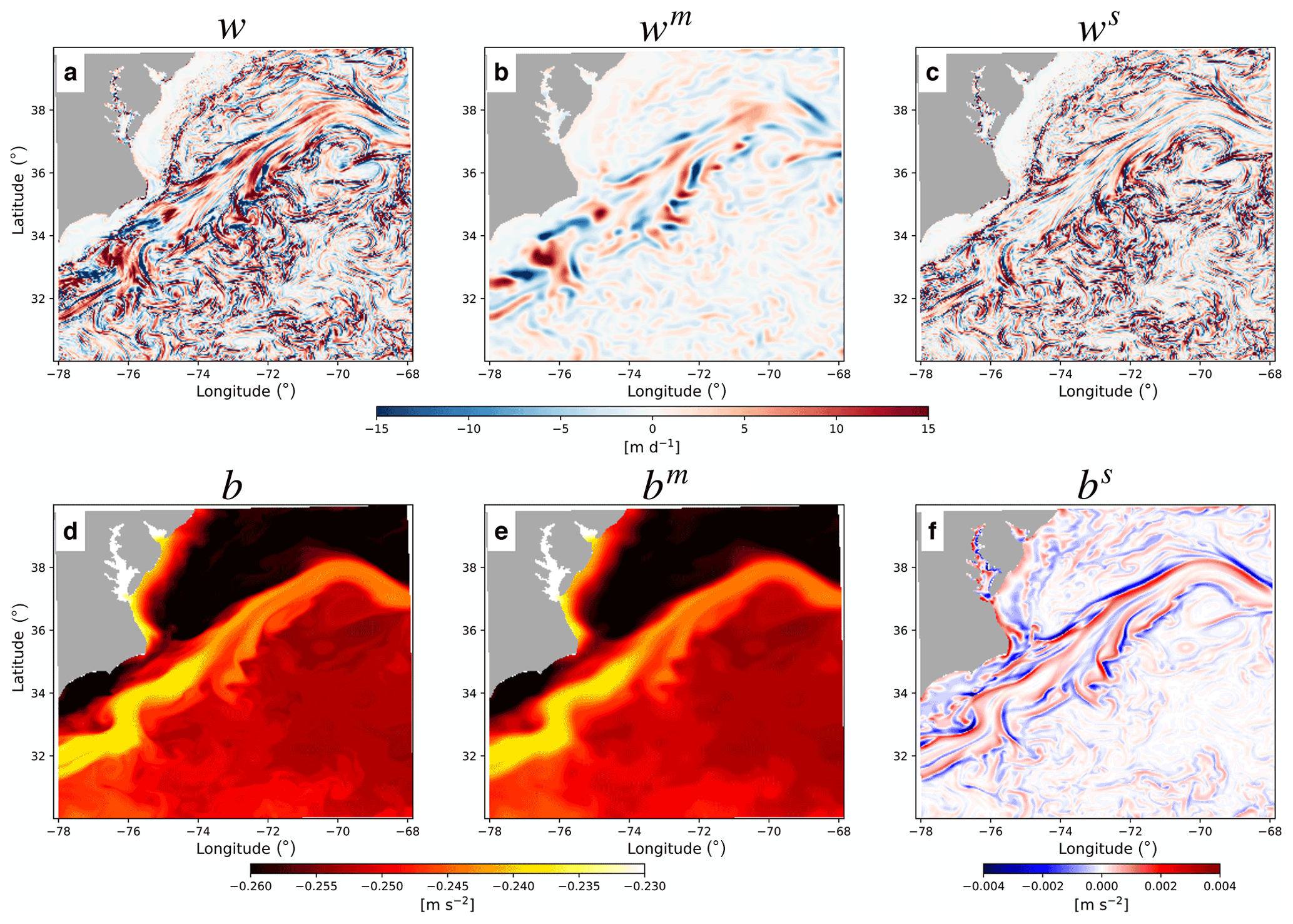
Figure 5Snapshot from eNATL60 on 1 February 2010 at depth 18 m of the unfiltered daily w and b (a, d), filtered fields applying the Gaussian filter (wm,bm; b, e), and the residual (ws,bs; c, f).
Considering that the Fox-Kemper et al. (2008) MLI parametrization is intended for mesoscale-permitting models (neglecting the dependency on model grid scale: Δs in Fox-Kemper et al., 2011), we further coarse-grained the fields to ∘ with a box-car operator, which gives
where 〈⋅〉 is the coarse-graining operator and Ce a tuning parameter or “efficiency coefficient” (Fox-Kemper et al., 2011). The Δs scaling to compensate for coarse model resolution was omitted due to all our model outputs partially resolving the submesoscale buoyancy flux. Furthermore, as Δs does not vary much among the models, this factor would not contribute much to the overall differences between models in comparison to the greater variability due to numerics, etc., that this paper is meant to introduce. We diagnosed Ce by taking the ratio between the right-hand and left-hand sides of Eq. (2) at each grid point and time step (e.g., left columns of Fig. E1) and then the horizontal spatial median of it. The diagnosis (Eq. 2) would differ from the parametrization (Eq. 1) if there are large vertical variations in the buoyancy gradient, but these are not expected within the frequently remixed mixed layer. Furthermore, the efficiency coefficient is expected to vary among the multi-model ensemble according to how well-resolved and/or damped the submesoscale instabilities are by model numerics, sub-grid schemes, and daily averaging.
The diagnosed Ce only has a time dependence and fluctuates in the range of [0.01,0.07] across most models (blue solid curves in Fig. 6), in agreement with the value of 0.06 recommended by Fox-Kemper et al. (2008). The time series of the spatial median of and its prediction from the MLI parametrization are in sync with each other (black and red solid curves in Fig. 6). The order of magnitude of the spatial median of the submesoscale vertical buoyancy flux diagnosed from the models, m2 s−3), also agrees with observational estimates (Mahadevan et al., 2012; Johnson et al., 2016; Buckingham et al., 2019), with an overall decrease in amplitude towards May except for FIO-COM32, which shows a local maximum around March (black solid curves in Fig. 6).
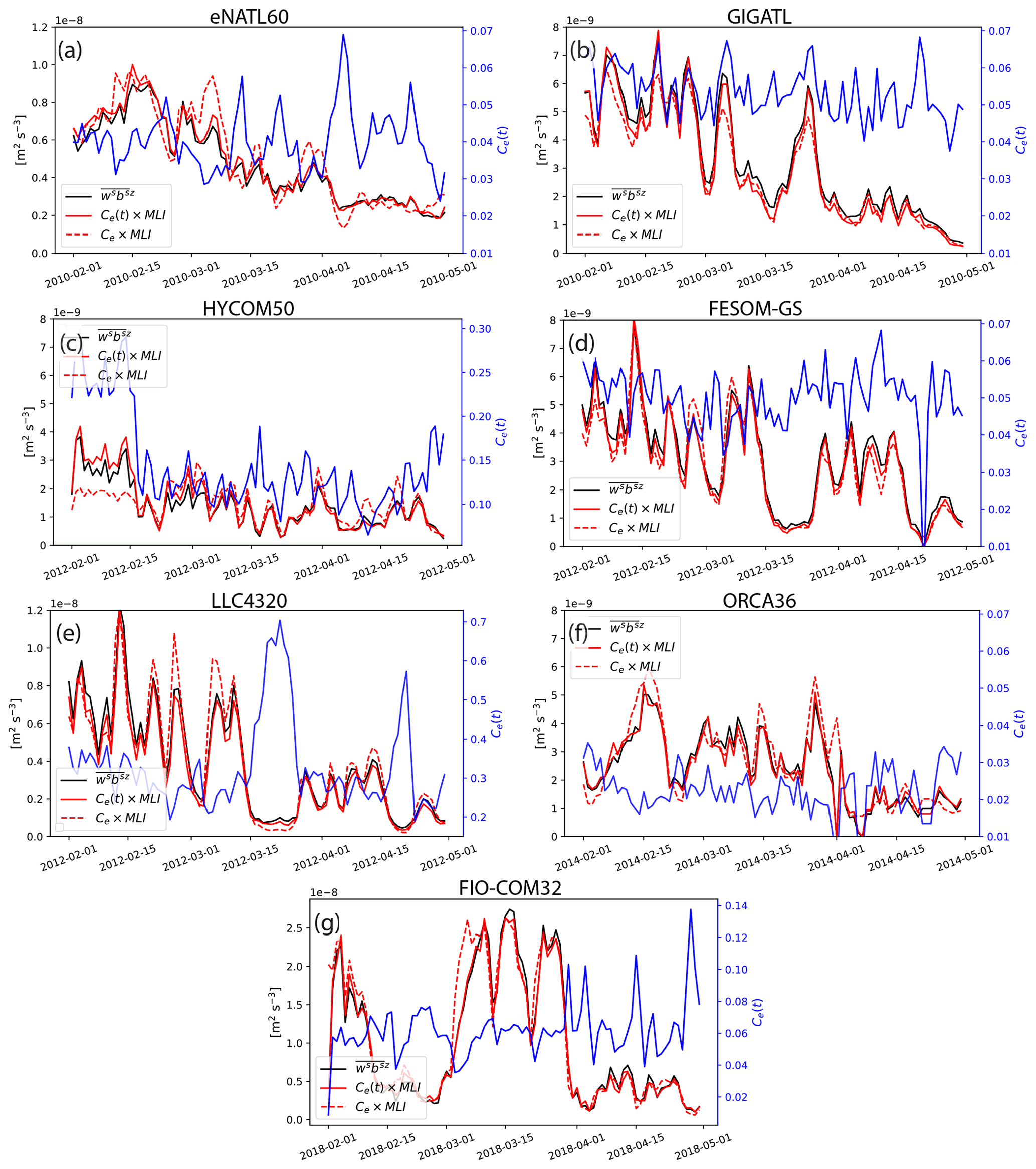
Figure 6Time series of the spatial median of the submesoscale vertical buoyancy flux averaged over the MLD (; black solid curve) and its prediction from the MLI parametrization during the months of February to April. Note that the y axes vary depending on the magnitude diagnosed from each simulation in order to highlight its temporal variability. The prediction with temporally varying Ce(t) is shown in red solid curves and with a temporally averaged (constant) Ce in red dashed curves. Ce(t) is plotted against the right y axes in blue. Three-dimensional data were not available for HYCOM25.
We provide a snapshot of and its prediction from the MLI parametrization (i.e., both sides of Eq. 2) on 1 February from each model in Fig. 7. The joint histograms of the two over the months of February–April are also given in the bottom rows of Fig. 7. The joint histograms of the two are concentrated around the one-to-one line indicating spatial correlation. The slight underestimation of magnitude in the MLI parametrization (viz. values falling below the one-to-one line) comes from the fact that, while can take negative values locally where frontogenesis dominates (i.e., where the isopycnals steepen), the MLI parametrization by construction cannot differentiate between frontogenesis and frontolysis, giving only positive values (Eq. 1). Nonetheless, largely takes positive values, indicating that processes such as mixed-layer and symmetric instabilities, which yield positive vertical buoyancy fluxes consistent with the extraction of potential energy (Dong et al., 2021), dominate in the surface boundary layer. While we have taken the spatial median to diagnose Ce(t), which yields the best agreement in the time series (Fig. 6), one may decide to instead take the spatial mean or mode, which we discuss in Appendix E.
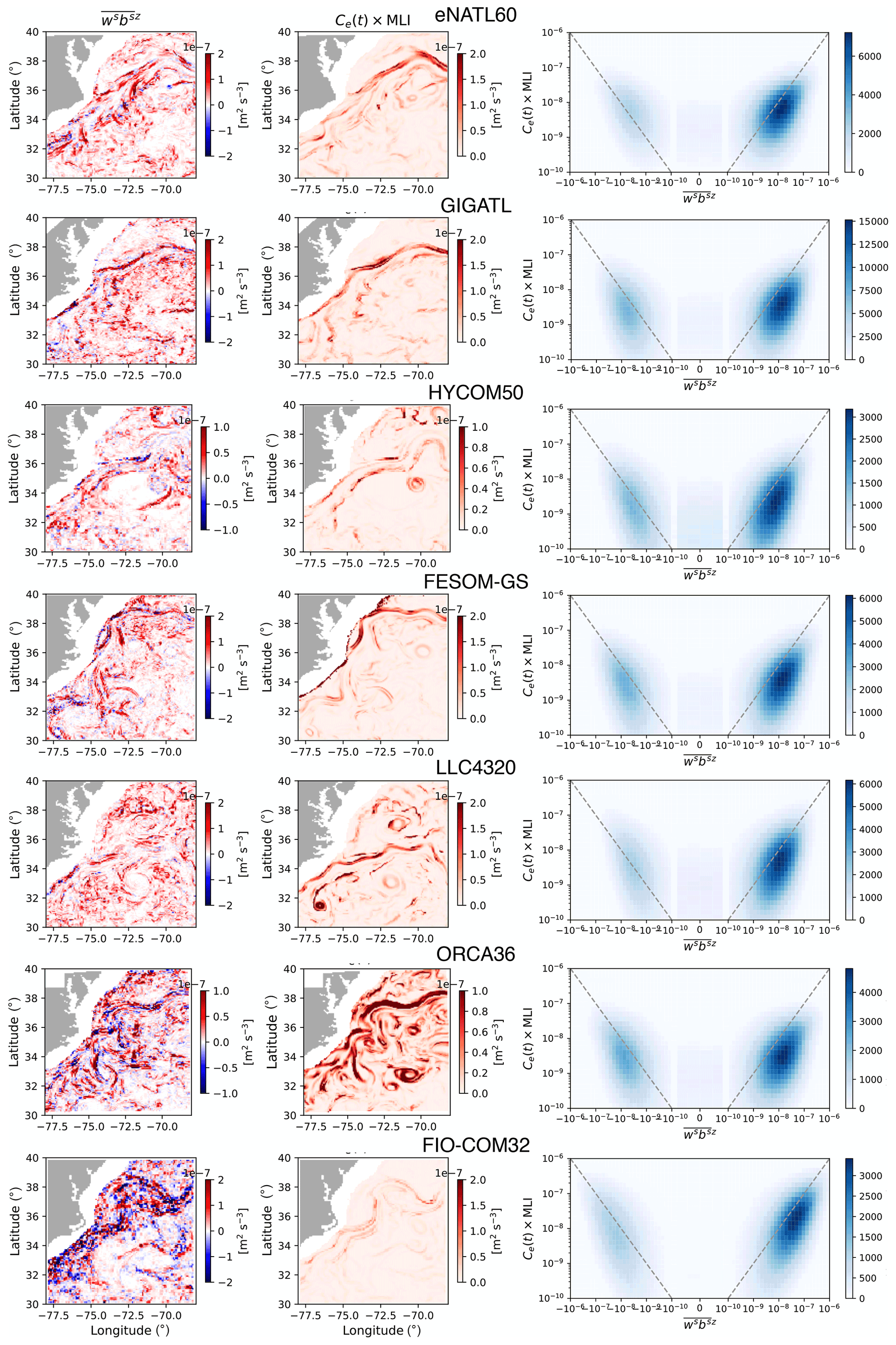
Figure 7Snapshot of (left column) and Ce(t)×MLI (middle column) on 1 February for each model. Note that the range of the color bar differs depending on the magnitude diagnosed from each model to highlight their spatial features and comparison between the submesoscale buoyancy flux and its equivalent predicted from the parametrization per simulation. Regions with bathymetry shallower than 100 m are masked out. The right column for each model shows the joint histogram of the two during the months of February to April, and the one-to-one line is shown as the grey dashed line. The histograms were computed using the xhistogram Python package (Abernathey et al., 2021c).
For operational purposes, we would like to have a tuning parameter that is independent of not only space, but also time. Therefore, we also display the MLI prediction when Ce is a constant taken to be its time mean. The agreement between and the prediction remains surprisingly good (red dashed curves in Fig. 6); in other words, the MLI parametrization is relatively insensitive to the temporal variability of Ce(t). Regarding inter-model differences, HYCOM50 and LLC4320 have the smallest buoyancy fluxes predicted by the MLI parametrization (i.e., weaker horizontal gradient magnitude and/or shallower MLDs). The smaller predicted values present themselves as Ce diagnosed from the two, taking an order of magnitude larger values than the other models (blue curves in Fig. 6c and e); particularly for HYCOM50, using a constant Ce fails to reproduce the magnitude of during the early half of February (red dashed curve in Fig. 6c). It is possible that the lowest vertical resolution of HYCOM50 amongst the models (Table B2) results in underrepresentation of the MLD despite its fine horizontal resolution, particularly south of the Gulf Stream (Fig. D1c); the MLI parametrization depends on it quadratically (Eq. 1). The MLD from LLC4320 is also relatively shallow (Fig. D1e). HYCOM50 and LLC4320 both use the K-profile parametrization (KPP, Table B3; Large et al., 1994) for the boundary-layer closure, which may imply that the KPP parameters warrant further tuning or reformulation for submesoscale-permitting model resolutions (e.g., Bachman et al., 2017; Souza et al., 2020). The shallow MLD may also be due to the differences in the atmospheric products used to force the models (Table B6).
The strength of cloud storage and computing comes from it being decentralized from any specific institution, but this also leaves open the question about who pays for the cost of operating and supporting the cloud infrastructure as well as for the cloud resources. There are three components to the cost structure: (i) the cloud storage, (ii) computation including egress charges to access the data, and (iii) deployment and maintenance of JupyterHub.
Currently, as of writing, the operational cost of fluxing data to the OSN cloud storage is funded by an NSF grant acquired by the Climate Data Science Laboratory at Columbia University and JupyterHub on Google Cloud Platform (GCP) by a Centre National d'Études Spatiales (CNES) grant acquired by the MultiscalE Ocean Modeling (MEOM) group at the Institut des Géosciences de l'Environnement. While the OSN storage itself allocated to Pangeo Forge is not associated with monetary expense or any egress charges (https://www.openstoragenetwork.org/get-involved/get-an-allocation/, last access: 8 July 2022), the scratch storage on GCP where we have saved our diagnostic outputs entailed storage and egress fees. The cost of GCP resources for JupyterHub with parallelized computation added up to roughly EUR 1000 per month for this study with the maximum computational resources of 64 cores and 256 Gb of memory per user; the resources scale on demand. As of writing, we have consumed 3.5 tera-hours of CPU and 92.1 Tb of RAM monthly on average. The operational scale of EUR 1000 per month worth of GCP credits, including the scratch storage and egress charges, was too small for us to directly contract with Google, so we have gone through a private broker in acquiring the GCP contract. (Our contract with the broker was an additional EUR 600 per month.) The cost of operating the scalable Kubernetes infrastructure is managed by a non-profit vendor (2i2c) for an additional few thousand dollars a month (https://docs.2i2c.org/en/latest/about/pricing/index.html, last access: 8 July 2022; we note that the operational cost somewhat depends on the contract negotiated amongst the party of interest, the cloud vendor, and 2i2c).
Although the net cost of a few thousand Euros per month may seem expensive compared to the local download framework where the costs of computation are shouldered upfront upon purchase of the cluster, there are several benefits to a cloud-based approach. First, using cloud infrastructure shifts the burden of hardware maintenance to the cloud provider, and users benefit from regular updates to technology and services that are available, meaning the scientific community can benefit from industry-driven innovations. Second, cloud infrastructure can be managed remotely and may use an inter-operable stack based on standards that are supported by many cloud providers (such as open-source tools like Kubernetes and JupyterHub). As all of the underlying technology is open source, it is technically possible for us to have deployed the Kubernetes infrastructure on our own. However, as Earth scientists, we often do not possess the adequate software engineering skills, and such expertise is highly sought after by industry; the hiring of a software engineer at public and higher-educational institutions is difficult due to financial constraints. The service provided by 2i2c makes it easier to port workflows between clouds and get more cost-effective support in operating this infrastructure compared to paying full-time software engineers who run local hardware for an institution.
We would like to note that, while we have chosen GCP and OSN for the cloud platform, the core design principles and technology behind Pangeo Forge and JupyterHub operated by 2i2c are non-proprietary and cloud vendor agnostic (for example, as defined in 2i2c's “Right to Replicate”; https://2i2c.org/right-to-replicate, last access: 8 July 2022). We could re-deploy the entire cloud platform on a different cloud provider with relative ease. This lets the users of this platform benefit from the flexibility and efficiency of the cloud while minimizing the risk of lock-in and dependence on proprietary technology. As the cloud-based framework spreads within the scientific community, it is also possible that the ocean and climate science community will be able to negotiate better deals with cloud service providers; the framework is apt for OMIP and Coupled Model Intercomparison Project (CMIP) (Griffies et al., 2016; Eyring et al., 2016) studies where terabytes and petabytes of data need to be shared and analyzed consistently. The systematic storage of ARCO data with open-access and appropriate cataloging will also enable reproducible science, a crucial step when evaluating newer simulations against previous runs. While we believe we have provided a proof of concept that cloud computing can be implemented with open-source technologies and can be leveraged for scientific research, the success of the framework will depend on the scientific community to convince its peers and funding organizations to recognize its benefit.
In this study, we have implemented a cloud-based framework for collaborative, open-source, and reproducible science and have showcased its potential by analyzing eight submesoscale-permitting simulations in a SWOT Xover region around the Gulf Stream separation (Region 1 in Fig. 1). We have shown that, despite the similar horizontal resolution amongst many models in this study, the spatial scales represented vary widely (Fig. 2). This diverse representation likely originates from differences in advective/diffusive schemes, boundary-layer parametrizations, atmospheric and tidal forcing, vertical resolution and/or bathymetry, and potentially duration of spinup amongst the simulations used here (Appendix B; cf. Chassignet and Xu, 2021). The need for collaborative work to inter-compare realistic simulations stems from both a scientific interest in the fidelity of submesoscale-permitting ocean models in representing the underlying physics and tracer transport and an engineering perspective on the numerics of ocean models. We leave a detailed analysis of the impact of numerics on the resolved dynamics for future work.
We have provided example diagnostics on SSH variability and submesoscale vertical buoyancy fluxes. The temporal standard deviation and spectra of SSH were significantly lower for the simulations without tidal forcing compared to the tidally forced simulations (Figs. 3 and 4). This implies that, in order to emulate the upcoming SWOT altimetric observations, tidal forcing is a key factor in modeling the surface ocean (Savage et al., 2017a, b; Arbic et al., 2018; Yu et al., 2021; Barkan et al., 2021; Le Guillou et al., 2021). Regarding 3D diagnostics, both the good agreement across multiple models between the tuning parameter Ce in the MLI parametrization and the values recommended by its developers (Fig. 6; Fox-Kemper et al., 2008; Fox-Kemper and Ferrari, 2008) and the consistency of the order of magnitude of the flux predicted by the parametrization in the spatially averaged sense with observational estimates (cf. Richards et al., 2021) combine to provide confidence in implementing the MLI parametrization in realistic ocean and climate models. This is in contrast, however, to a recent study by Yang et al. (2021, their Fig. 7), where they found (using the Regional Ocean Modeling System, ROMS, with KPP) that the time series of did not correlate well with the prediction from its parametrization in the Kuroshio extension. While we lack access to their model outputs, we speculate that the differences could be due to the diagnostic methods, domain of interest, and/or configuration of their simulation. The contrasting findings all the more highlight the need for collaborative and open data analysis strategies of multi-model ensembles in assessing and improving the simulations themselves. We would like to note that were the modeled domain by Yang et al. (2021) to cover Region 1, the cloud-based framework would allow for a straightforward platform to extend the ensemble of simulations (Appendix B) to include their outputs for our inter-comparison and reproducible science.
We end by noting that cloud-based data-proximate computation provides a framework to systematically analyze terabytes and petabytes of data as we further increase the resolution and complexity of ocean and climate simulations and as SWOT data become available. However, the success of the framework will depend on the ability of scientists to convince funding organizations to recognize its potential. Cloud-based computing differs from the conventional workflow, which involves funding of local computational resources and storage. While the cloud-based framework does not allow for an individual researcher or group to have prioritized access over the data and analytical tools, we believe that open access to the data will allow for reproducible science and facilitate international collaboration.
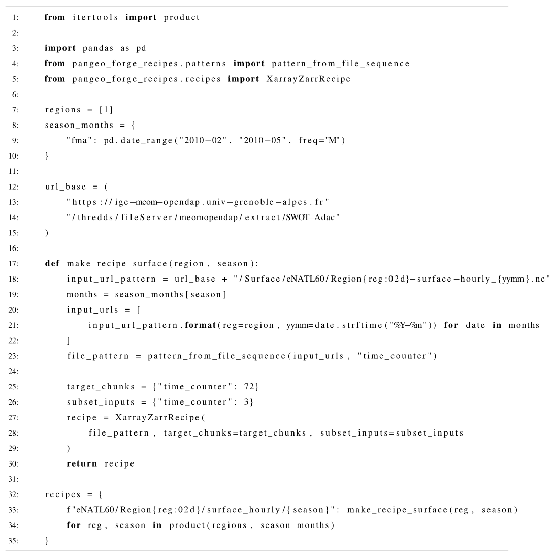
pangeo_forge_recipe for eNATL60 Here we provide the Pangeo Forge recipe used to flux eNATL60 surface hourly data to OSN for Region 1 during February and April 2010.
The input_url_pattern is where the original NetCDF files were hosted on an OPeNDAP server, upon which the files were chunked along the time dimension before being fluxed to the cloud in zarrified format (Miles et al., 2020). As a contributor to Pangeo Forge, one essentially only needs to specify the input_url_pattern. The zarrification and fluxing of the data to the cloud are automated by Pangeo Forge, reducing the infrastructure and cognitive burden on the data provider (Stern et al., 2022a).
We provide the model configurations in Tables B1–B6 (blanks indicate the information was not obtainable).
The vertical coordinate transformation onto geopotential coordinates for the outputs of GIGATL and HYCOM50, which had terrain-following and isopycnal coordinates as their native grid, respectively (Table B2), were done using the xgcm Python package (Abernathey et al., 2021b) with linear interpolation.
For the sake of storage, only 3 months of output for summer (August, September, October) and winter (February, March, April), respectively, are stored on OSN from an arbitrary year per simulation.
Table B1The model and initial condition used for each simulation and their duration of spinup and year of output stored on OSN. HYCOM50 was spun up from the rest and integrated for a total of 20 years. Sensitivity experiments were performed starting from year 15 (Chassignet and Xu, 2017, 2021). LLC4320 used progressive spinup from a ∘ state estimate (Menemenlis et al., 2008) followed by and ∘ simulations, as detailed in Table D2 of Rocha et al. (2016).
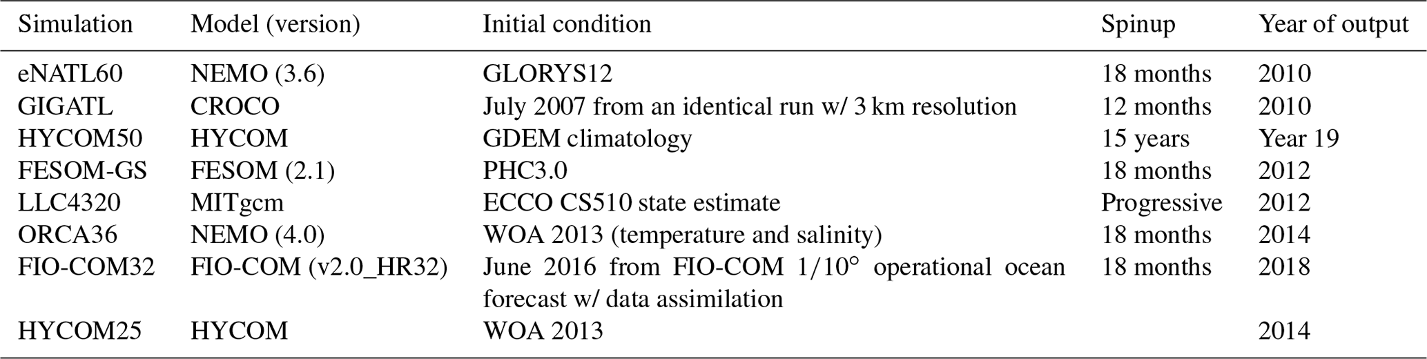
Table B2The horizontal and vertical native coordinate system, spatial resolution, and domain coverage for each simulation. The Z* vertical coordinate is the rescaled geopotential coordinate where the fluctuations of the free surface are taken into account (cf. Griffies et al., 2016). Note that vertical resolution as well as horizontal resolution vary significantly between the models. Outputs from FESOM-GS were interpolated onto a Cartesian grid offline with a cubic spline.

Table B3The equation of state (EOS), surface boundary layer (SBL) parametrization used, and tidal forcing in each simulation. * Jackett and McDougall (1995, JMD95) in HYCOM is implemented with the approximation by Brydon et al. (1999). The potential densities were computed following each EOS with the reference pressure of 0 dbar (Fernandes, 2014; Abernathey, 2020; Firing et al., 2021). The EOS for FIO-COM32 is available on Github (Stern et al., 2022b, https://github.com/pangeo-data/swot_adac_ogcms, last access: 8 July 2022). Note that FESOM-GS and ORCA36 do not have tidal forcing, whilst the others have at least the leading five tidal forcings.
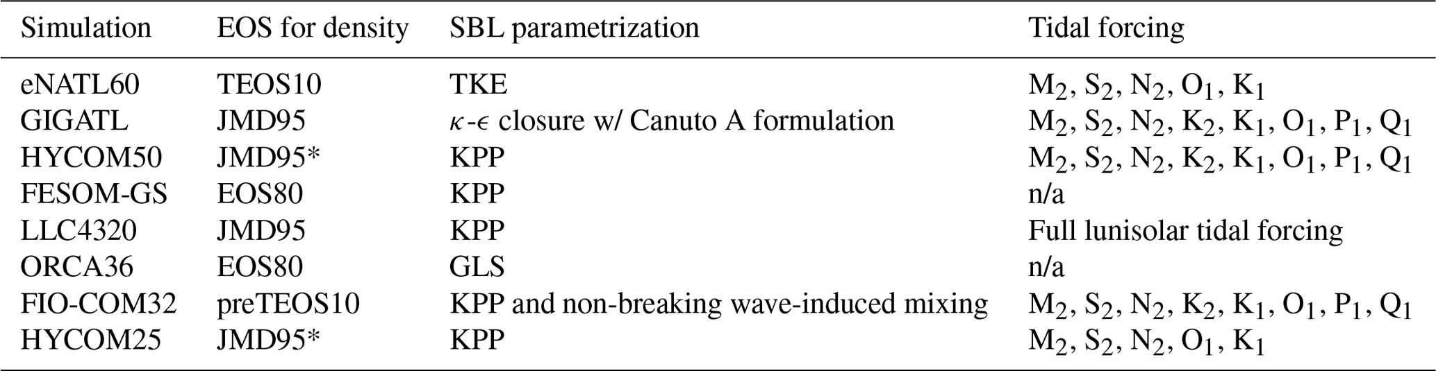
n/a: not applicable
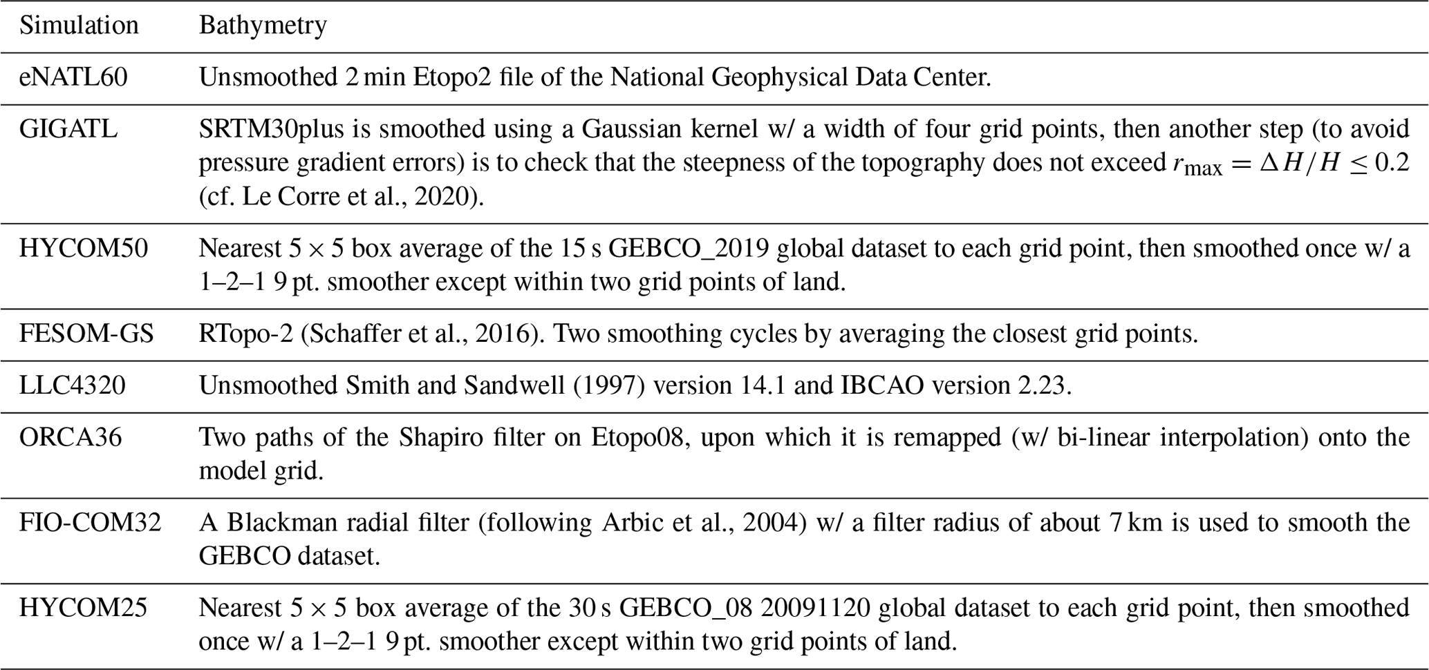
Table B5The advection and dissipation schemes used for each simulation. Note that some models have biharmonic viscosities and others do not.
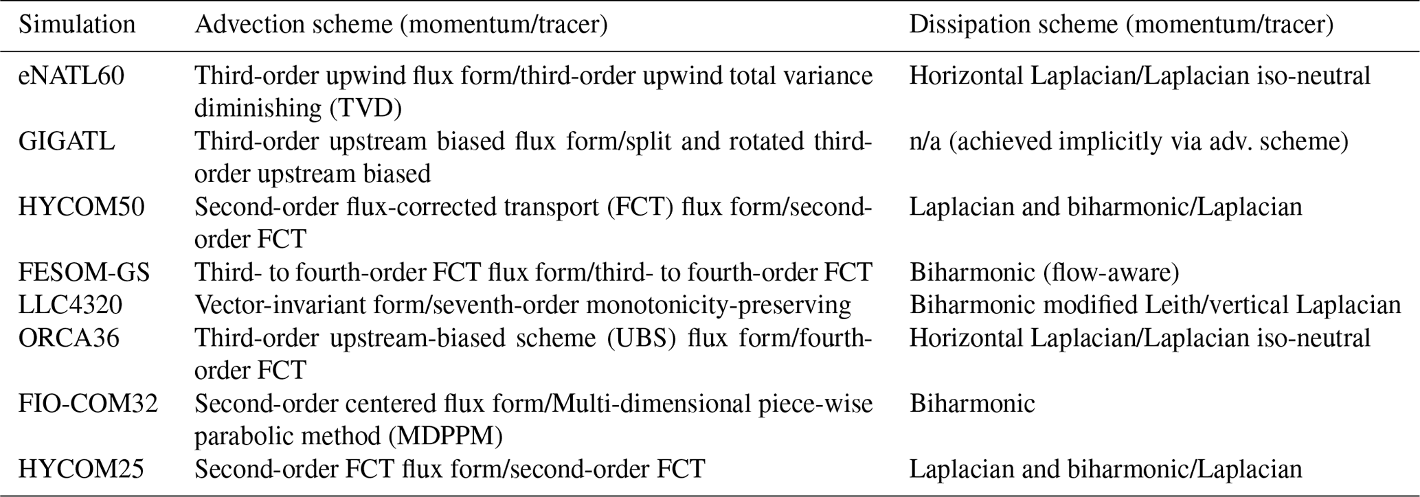
n/a: not applicable
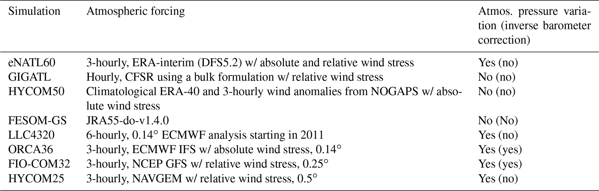
Table B6The atmospheric forcing and the inclusion of atmospheric pressure variation at the surface.
In this Appendix, we examine the effect of spatiotemporal filtering on the modeled SSH standard deviation. In order to mimic a smoothing procedure similar to the AVISO products, we apply a Gaussian spatial filter with the standard deviation of 50 km using the gcm-filters Python package and a 10 d running mean (cf. Chassignet and Xu, 2017).
The non-tidally forced runs do not show much difference upon spatiotemporal smoothing from their standard deviation using hourly outputs, but they significantly decrease for the tidally forced runs, particularly LLC4320 and FIO-COM32, with the modeled amplitudes coming closer to the AVISO estimate (Figs. 3 and C1). The strong reduction in LLC4320 and FIO-COM32 may be expected as they are the runs with the highest SSH variance at frequencies higher than the Coriolis frequency (Fig. 4). All simulations agree that there is a local maximum in standard deviation around 37∘ N, where the separated GS is situated, consistent with AVISO. The SSH variability in GIGATL may be on the lower end considering that it is tidally forced (Fig. C1b), which could also be due to the lack of pressure variation in the atmospheric forcing (Table B6).

The MLD averaged between 1 and 15 February is shown in Fig. D1 along with the climatology for the month of February estimated from the Argo floats. We see that the MLDs from HYCOM50 and LLC4320 are notably shallower south of the Gulf Stream compared to the other models and Argo estimates.
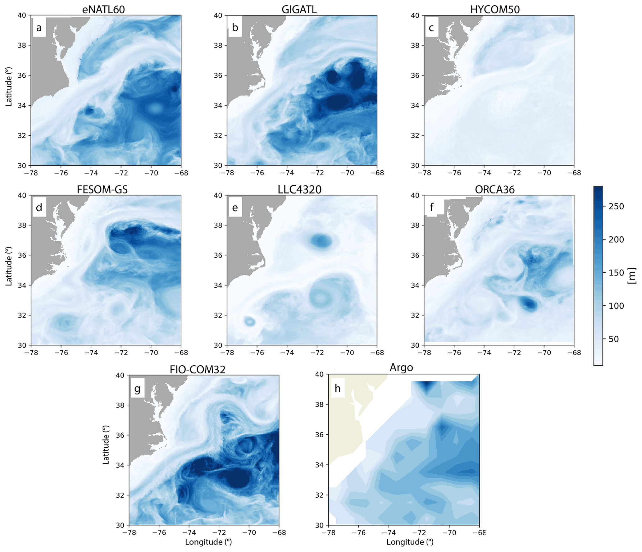
Figure D1MLD from each model averaged over the duration of 1–15 February when the prediction from the MLI parametrization with a constant Ce in HYCOM50 deviates from the diagnosed submesoscale vertical buoyancy flux. The MLD was defined using the density criteria of de Boyer Montégut et al. (2004). For models with non-geopotential vertical coordinates (i.e., GIGATL and HYCOM50), the MLD was computed using their native coordinates, respectively. The climatology for the month of February from the Argo floats is taken from the dataset by Holte et al. (2017). The monthly-mean MLD defined by the density criterion (mld_dt_mean) is shown in order to be consistent with our model estimates.
The efficiency coefficient diagnosed from each simulation is given in the left column of Fig. E1 and the joint histogram where Ce(t) is taken as the spatial mean and mode in the right two columns, respectively. It is interesting to note that tends to take small values within fronts (namely, where the magnitude of is large) but takes large values, reaching up to O(1), on their periphery (Figs. 7 and E1). Comparing the joint histograms in Figs. 7 and E1, taking the spatial mean to diagnose Ce(t) tends to overestimate the flux magnitude predicted from the parametrization as the mean is more sensitive to extrema than the median; the histograms are concentrated above the one-to-one line (middle column of Fig. E1). Diagnosing Ce(t) as the spatial mode seemingly improves the alignment of the histogram with the one-to-one line (right column of Fig. E1). However, taking the spatial mode results in Ce(t) reaching values up to 2 orders of magnitude larger than the values recommended by Fox-Kemper et al. (2008), and the time series predicted from the parametrization results in overestimation of the submesoscale buoyancy flux in the spatially averaged sense (Fig. E2). The time series predicted from using the spatial mean to estimate Ce(t) further overestimates the buoyancy flux (not shown). We, therefore, recommend the usage of the spatial median in estimating Ce(t).
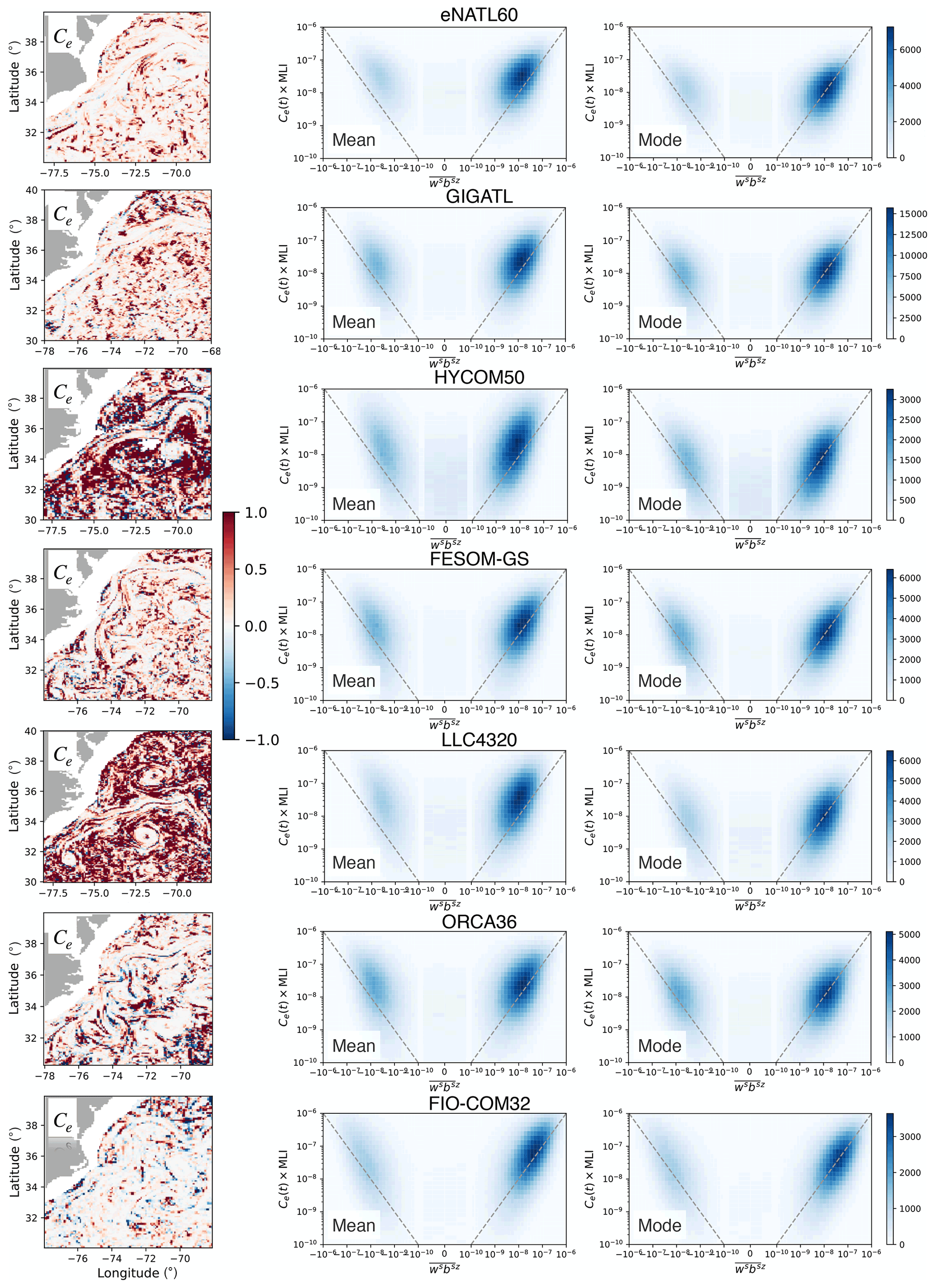
Figure E1Snapshot of the efficiency coefficient diagnosed on 1 February from each simulation (left column). The joint histogram of and Ce(t)×MLI during the months of February to April (right columns). The middle column shows the histogram when Ce(t) is taken as the spatial mean of and the right column as the spatial mode of . The one-to-one line is shown as the grey dashed line.
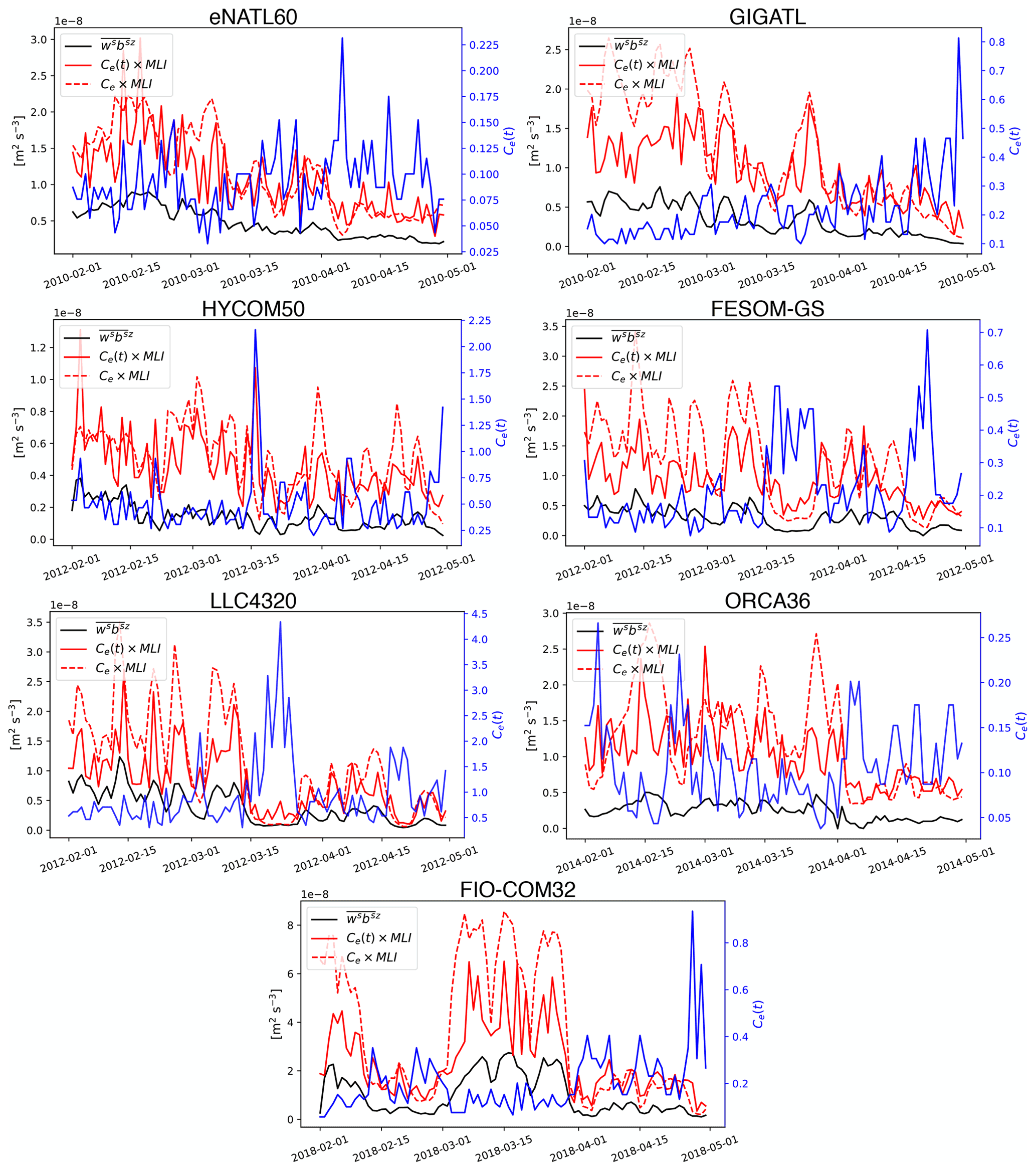
Figure E2Time series of the spatial median of the submesoscale vertical buoyancy flux averaged over the MLD (; black solid curve) and its prediction from the MLI parametrization during the months of February to April, where Ce(t) is taken as the spatial mode of . Note that the y axes vary depending on the magnitude diagnosed from each simulation in order to highlight its temporal variability. The prediction with temporally varying Ce(t) is shown in red solid curves and with a temporally averaged (constant) Ce in red dashed curves. Ce(t) is plotted against the right-hand-side y axes in blue.
The model outputs from eNATL60, GIGATL, HYCOM50, FESOM-GS, ORCA36, FIO-COM32, and HYCOM25 at the SWOT Xover regions are all publicly available on the Open Storage Network (OSN). The Jupyter notebooks and Yaml file used to access and analyze the data are available on Github (Stern et al., 2022b, https://github.com/pangeo-data/swot_adac_ogcms, last access: 8 July 2022, and https://doi.org/10.5281/zenodo.6762536).
The LLC4320 data were accessed via the NASA ECCO Data Portal (https://data.nas.nasa.gov/ecco/data.php?dir=/eccodata/llc_4320, last access: 8 July 2022) using the llcreader of the xmitgcm Python package (Abernathey et al., 2021d; Abernathey, 2019). The raw model outputs of eNATL60 and GIGATL are available at https://doi.org/10.5281/zenodo.4032732 (Brodeau et al., 2020) and https://doi.org/10.5281/zenodo.4948523 (Gula et al., 2021).
The conceptualization of this project was by TU and JLS; methodology by TU; software development by TU, AA, LB, CS, RPA and CH; validation by TU; formal analysis by TU; investigation by TU, JLS, BFK and WKD. Computational resources were acquired by JLS and RPA; data curation of running the simulations was done by JLS, AA, LB, EPC, XX, JG, GR, NK, SD, QW, DM, CB, BKA, JFS, FQ, BX, AB, RS and AW; writing of the manuscript by TU; visualization of the figures by TU; project administration by JLS; funding acquisition for the project by JLS and RPA.
The contact author has declared that none of the authors has any competing interests.
Publisher's note: Copernicus Publications remains neutral with regard to jurisdictional claims in published maps and institutional affiliations.
We thank the editor Riccardo Farneti and Stephen Griffies, Mike Bell, Andy Hogg, and Joel Hirschi for their reviews. Takaya Uchida was supported by the French “Make Our Planet Great Again” (MOPGA) initiative managed by the Agence Nationale de la Recherche (ANR) under the Programme d'Investissement d'Avenir, with the reference ANR-18-MPGA-0002. This work is a contribution to the Consistent OceaN Turbulence for ClimaTe Simulators (CONTaCTS) project and SWOT mission Science Team (https://www.swot-adac.org/, last access: 8 July 2022).
Julien Le Sommer, Laurent Brodeau, and Aurélie Albert thank the PRACE 16th call project ReSuMPTiOn (Revealing SubMesoscale Processes and Turbulence in the Ocean, P.I. Laurent Brodeau) for awarding access to the MareNostrum supercomputer at the Barcelona Supercomputing Center.
Operational costs for the cloud-based JupyterHub were funded by CNES through their participation in the SWOT Science Team.
Ryan P. Abernathey and Charles Stern were supported by NSF award 2026932 for the development of Pangeo Forge and OSN storage. This study is a contribution to projects S2: Improved parameterisations and numerics in climate models (Sergey Danilov), S1: Diagnosis and Metrics in Climate Models (Nikolay Koldunov), and M5: Reducing spurious diapycnal mixing in ocean models (Sergey Danilov) of the Collaborative Research Centre TRR 181 “Energy Transfer in Atmosphere and Ocean” funded by the Deutsche Forschungsgemeinschaft (DFG, German Research Foundation) – project no. 274762653 – and the Helmholtz initiative REKLIM (Regional Climate Change; Qiang Wang).
Brian K. Arbic and Jay F. Shriver were supported by NASA grant 80NSSC20K1135. Eric P. Chassignet and Xiaobiao Xu were supported by ONR grants N00014-19-1-2717 and N00014-20-1-2769.
Baylor Fox-Kemper was supported by ONR N00014-17-1-2963 and NOAA NA19OAR4310366. Fangli Qiao and Bin Xiao were supported by the National Natural Science Foundation of China with grant no. 41821004.
Clément Bricaud was supported by EU H2020 projects IMMERSE (grant agreement no. 821926) and ESIWACE2 (grant agreement no. 823988). Jonathan Gula is grateful for support from the ANR through the DEEPER project (ANR‐19‐CE01‐0002‐01). Jonathan Gula and Guillaume Roullet thank PRACE and GENCI for awarding access to HPC resources Joliot-Curie Rome and SKL from GENCI-TGCC (grants 2020-A0090112051 and 2019gch0401 and PRACE project 2018194735) and HPC facility DATARMOR of “Pôle de Calcul Intensif pour la Mer” at Ifremer, Brest, France. William K. Dewar was supported by NSF grants OCE-182956 and OCE-2023585.
Dimitris Menemenlis carried out research at the Jet Propulsion Laboratory, California Institute of Technology, under contract with NASA, with support from the Physical Oceanography and Modeling, Analysis, and Prediction Program. High-end computing was provided by NASA Advanced Supercomputing at Ames Research Center. We would like to thank 2i2c.org (https://2i2c.org/, last access: 8 July 2022) for deploying and maintaining JupyterHub on the Google Cloud Platform and the NASA ECCO team for maintaining the data portal through which the LLC4320 data were accessed. We thank Stack Labs for brokering the GCP contract.
The altimeter products were produced by Ssalto/Duacs and distributed by Aviso+ with support from CNES (https://www.aviso.altimetry.fr, last access: 8 July 2022). The geographic figures were generated using the Cartopy Python package (Met Office, 2010–2015).
This research has been supported by the Agence Nationale de la Recherche (grant nos. ANR-18-MPGA-0002 and ANR‐19‐CE01‐0002‐01), the National Science Foundation (grant nos. 2026932, OCE-182956, and OCE-2023585), the Deutsche Forschungsgemeinschaft (grant no. 274762653), the National Aeronautics and Space Administration (grant no. 80NSSC20K1135), the Office of Naval Research (grant nos. N00014-19-12717, 13034596, and N00014-17-1-2963), the National Oceanic and Atmospheric Administration (grant no. NA19OAR4310366), the National Natural Science Foundation of China (grant no. 41821004), the Partnership for Advanced Computing in Europe AISBL (ReSuMPTiOn; grant no. 2018194735), the European Commission, Horizon 2020 (IMMERSE, grant no. 821926, and ESiWACE2, grant no. 823988), and the Grand Équipement National De Calcul Intensif (grant nos. 2020-A0090112051 and 2019gch0401).
This paper was edited by Riccardo Farneti and reviewed by Stephen M. Griffies, Mike Bell, Joel Hirschi, and Andy Hogg.
Abernathey, R. P.: Petabytes of Ocean Data, Part I: NASA ECCO Data Portal, https://medium.com/pangeo/petabytes-of-ocean-data-part-1-nasa-ecco-data-portal-81e3c5e077be (last access: 8 July 2022), 2019. a, b
Abernathey, R. P.: fastjmd95: Numba implementation of Jackett &
McDougall (1995) ocean equation of state, Zenodo [code], https://doi.org/10.5281/zenodo.4498376,
2020. a
Abernathey, R. P., Augspurger, T., Banihirwe, A., Blackmon-Luca, C. C., Crone, T. J., Gentemann, C. L., Hamman, J. J., Henderson, N., Lepore, C., McCaie, T. A., Robinson, N. H., and Signell, R. P.: Cloud-Native Repositories for Big Scientific Data, Comput. Sci. Eng., 23, 26–35, https://doi.org/10.1109/MCSE.2021.3059437, 2021a. a, b
Abernathey, R. P., Busecke, J., Smith, T., et al.: xgcm: General Circulation Model Postprocessing with
xarray, Zenodo [code], https://doi.org/10.5281/zenodo.3634752, 2021b. a, b
Abernathey, R. P., Dougie, S., Nicholas, T., Bourbeau, J., Joseph, G., Yunyi,
Y., Bailey, S., Bell, R., and Spring, A.: xhistogram: Fast, flexible,
label-aware histograms for numpy and xarray, Zenodo [code], https://doi.org/10.5281/zenodo.5757149,
2021c. a
Abernathey, R. P., Dussin, R., Smith, T., et al.: xmitgcm: Read
MITgcm mds binary files into xarray, Zenodo [code], https://doi.org/10.5281/zenodo.596253,
2021d. a
Ajayi, A., Le Sommer, J., Chassignet, E., Molines, J.-M., Xu, X., Albert, A., and Dewar, W. K.: Diagnosing cross-scale kinetic energy exchanges from two submesoscale permitting ocean models, J. Adv. Model. Earth Sy., 13, 6, https://doi.org/10.1029/2019MS001923, 2021. a, b
Arbic, B. K., Garner, S. T., Hallberg, R. W., and Simmons, H. L.: The accuracy of surface elevations in forward global barotropic and baroclinic tide models, Deep-Sea Res. Pt. II, 51, 3069–3101, https://doi.org/10.1016/j.dsr2.2004.09.014, 2004. a
Arbic, B. K., Polzin, K. L., Scott, R. B., Richman, J. G., and Shriver, J. F.: On eddy viscosity, energy cascades, and the horizontal resolution of gridded satellite altimeter products, J. Phys. Oceanogr., 43, 283–300, https://doi.org/10.1175/JPO-D-11-0240.1, 2013. a
Arbic, B. K., Alford, M., Ansong, J., Buijsman, M., Ciotti, R., Farrar, J., Hallberg, R., Henze, C., Hill, C., Luecke, C., Menemenlis, D., Metzger, E., Müeller, M., Nelson, A., Nelson, B., Ngodock, H., Ponte, R., Richman, J., Savage, A., and Zhao, Z.: A primer on global internal tide and internal gravity wave continuum modeling in HYCOM and MITgcm, in: New Frontiers in Operational Oceanography, edited by: Chassignet, E., Pascual, A., Tintoré, J., and Verron, J., GODAE Ocean View, 307–392, https://doi.org/10.17125/gov2018.ch13, 2018. a, b, c
Bachman, S. D., Fox-Kemper, B., Taylor, J. R., and Thomas, L. N.: Parameterization of Frontal Symmetric Instabilities. I: Theory for Resolved Fronts, Ocean Model., 109, 72–95, https://doi.org/10.1016/j.ocemod.2016.12.003, 2017. a
Barham, W., Bachman, S., and Grooms, I.: Some effects of horizontal discretization on linear baroclinic and symmetric instabilities, Ocean Model., 125, 106–116, https://doi.org/10.1016/j.ocemod.2018.03.004, 2018. a
Barkan, R., Srinivasan, K., Yang, L., McWilliams, J. C., Gula, J., and Vic, C.: Oceanic mesoscale eddy depletion catalyzed by internal waves, Geophys. Res. Lett., 48, e2021GL094376, https://doi.org/10.1029/2021GL094376, 2021. a, b
Beg, M., Taka, J., Kluyver, T., Konovalov, A., Ragan-Kelley, M., Thiéry, N. M., and Fangohr, H.: Using Jupyter for reproducible scientific workflows, Comput. Sci. Eng., 23, 36–46, https://doi.org/10.1109/MCSE.2021.3052101, 2021. a
Bleck, R.: An oceanic general circulation model framed in hybrid isopycnic-Cartesian coordinates, Ocean Model., 4, 55–88, https://doi.org/10.1016/S1463-5003(01)00012-9, 2002. a
Boccaletti, G., Ferrari, R., and Fox-Kemper, B.: Mixed layer instabilities and restratification, J. Phys. Oceanogr., 37, 2228–2250, https://doi.org/10.1175/JPO3101.1, 2007. a, b, c
Bodner, A. S. and Fox-Kemper, B.: A breakdown in potential vorticity estimation delineates the submesoscale-to-turbulence boundary in large eddy simulations, J. Adv. Model. Earth Sy., 12, e2020MS002049, https://doi.org/10.1029/2020MS002049, 2020. a
Brannigan, L., Marshall, D. P., Naveira Garabato, A. C., Nurser, A. J. G., and Kaiser, J.: Submesoscale Instabilities in Mesoscale Eddies, J. Phys. Oceanogr., 47, 3061–3085, https://doi.org/10.1175/jpo-d-16-0178.1, 2017. a
Brodeau, L., Albert, A., and Le Sommer, J.: NEMO-eNATL60 description and assessment repository, Zenodo [data set], https://doi.org/10.5281/zenodo.4032732, 2020. a, b, c
Brydon, D., Sun, S., and Bleck, R.: A new approximation of the equation of state for seawater, suitable for numerical ocean models, J. Geophys. Res.-Oceans, 104, 1537–1540, https://doi.org/10.1029/1998JC900059, 1999. a
Buckingham, C. E., Lucas, N., Belcher, S., Rippeth, T., Grant, A., Le Sommer, J., Ajayi, A. O., and Garabato, A. C. N.: The contribution of surface and submesoscale processes, J. Adv. Model. Earth Sy., 11, 12, https://doi.org/10.1029/2019MS001801, 2019. a
Callies, J. and Ferrari, R.: Note on the Rate of Restratification in the Baroclinic Spindown of Fronts, J. Phys. Oceanogr., 48, 1543–1553, https://doi.org/10.1175/jpo-d-17-0175.1, 2018. a
Calvert, D., Nurser, G., Bell, M. J., and Fox-Kemper, B.: The impact of a parameterisation of submesoscale mixed layer eddies on mixed layer depths in the NEMO ocean model, Ocean Model., 154, 101678, https://doi.org/10.1016/j.ocemod.2020.101678, 2020. a, b
Cao, H., Fox-Kemper, B., and Jing, Z.: Submesoscale Eddies in the Upper Ocean of the Kuroshio Extension from High-Resolution Simulation: Energy Budget, J. Phys. Oceanogr., 51, 2181–2201, https://doi.org/10.1175/JPO-D-20-0267.1, 2021. a
Chassignet, E. P. and Xu, X.: Impact of Horizontal Resolution (∘ to ∘) on Gulf Stream Separation, Penetration, and Variability, J. Phys. Oceanogr., 47, 1999–2021, https://doi.org/10.1175/JPO-D-17-0031.1, 2017. a, b, c, d, e
Chassignet, E. P. and Xu, X.: On the Importance of High-Resolution in Large-Scale Ocean Models, Adv. Atmos. Sci., 38, 1–14, https://doi.org/10.1007/s00376-021-0385-7, 2021. a, b, c, d
Chassignet, E. P., Hurlburt, H. E., Metzger, E. J., Smedstad, O. M., Cummings, J. A., Halliwell, G. R., Bleck, R., Baraille, R., Wallcraft, A. J., Lozano, C., Tolman, H. L., Srinivasan, A., Hankin, S., Cornillon, P., Weisberg, R., Barth, A., He, R., Werner, F., and Wilkin, J.: US GODAE: Global ocean prediction with the HYbrid Coordinate Ocean Model (HYCOM), Oceanography, 22, 64–75, 2009. a
Chassignet, E. P., Yeager, S. G., Fox-Kemper, B., Bozec, A., Castruccio, F., Danabasoglu, G., Horvat, C., Kim, W. M., Koldunov, N., Li, Y., Lin, P., Liu, H., Sein, D. V., Sidorenko, D., Wang, Q., and Xu, X.: Impact of horizontal resolution on global ocean–sea ice model simulations based on the experimental protocols of the Ocean Model Intercomparison Project phase 2 (OMIP-2), Geosci. Model Dev., 13, 4595–4637, https://doi.org/10.5194/gmd-13-4595-2020, 2020. a, b
Chelton, D. B., Schlax, M. G., and Samelson, R. M.: Global observations of nonlinear mesoscale eddies, Prog. Oceanogr., 91, 167–216, https://doi.org/10.1016/j.pocean.2011.01.002, 2011. a
Danilov, S., Sidorenko, D., Wang, Q., and Jung, T.: The Finite-volumE Sea ice–Ocean Model (FESOM2), Geosci. Model Dev., 10, 765–789, https://doi.org/10.5194/gmd-10-765-2017, 2017. a
de Boyer Montégut, C., Madec, G., Fischer, A. S., Lazar, A., and Iudicone, D.: Mixed layer depth over the global ocean: An examination of profile data and a profile-based climatology, J. Geophys. Res.-Oceans, 109, C12003, https://doi.org/10.1029/2004JC002378, 2004. a, b
Dong, J., Fox-Kemper, B., Zhang, H., and Dong, C.: The scale of submesoscale baroclinic instability globally, J. Phys. Oceanogr., 50, 2649–2667, https://doi.org/10.1175/JPO-D-20-0043.1, 2020. a, b
Dong, J., Fox-Kemper, B., Zhu, J., and Dong, C.: Application of symmetric instability parameterization in the Coastal and Regional Ocean Community Model (CROCO), J. Adv. Model. Earth Sy., 13, e2020MS002302, https://doi.org/10.1029/2020MS002302, 2021. a
Ducousso, N., Le Sommer, J., Molines, J.-M., and Bell, M.: Impact of the “Symmetric Instability of the Computational Kind” at mesoscale-and submesoscale-permitting resolutions, Ocean Model., 120, 18–26, https://doi.org/10.1016/j.ocemod.2017.10.006, 2017. a
Eyring, V., Bony, S., Meehl, G. A., Senior, C. A., Stevens, B., Stouffer, R. J., and Taylor, K. E.: Overview of the Coupled Model Intercomparison Project Phase 6 (CMIP6) experimental design and organization, Geosci. Model Dev., 9, 1937–1958, https://doi.org/10.5194/gmd-9-1937-2016, 2016. a
Fangohr, H., Beg, M., Bergemann, M., Bondar, V., Brockhauser, S., Carinan, C., Costa, R., Fortmann, C., Marsa, D. F., Giovanetti, G., Göries, D., Hauf, S., Hickin, D. G., Jarosiewicz, T., Kamil, E., Karnevskiy, M., Kirienko, Y., Klimovskaia, A., Kluyver, T. A., Kuster, M., Le Guyader, L., Madsen, A., Maia, L. G., Mamchyk, D., Mercadier, L., Michelat, T., Möller, J., Mohacsi, I., Parenti, A., Reiser, M., Rosca, R. Rueck, D. B ., Rüter, T., Santos, H., Schaffer, R., Scherz A., Scholz, M., Silenzi, A., Spirzewski, M., Sztuk-Dambietz, J., Szuba, J., Trojanowski, S., Wrona, K. Yaroslavtsev, A. A., Zhu, J., Rod, T. H., Selknaes, J. R., Taylor, J. W., Copenhagen, D. A., Campbell, A., Götz, J., and Kieffer, J.: Data exploration and analysis with jupyter notebooks, in: 17th Biennial International Conference on Accelerator and Large Experimental Physics Control Systems, TALK-2020-009, https://doi.org/10.18429/JACoW-ICALEPCS2019-TUCPR02, 2019. a
Fernandes, F.: python-seawater: Python re-write of the CSIRO seawater
toolbox SEAWATER-3.3 for calculating the properties of sea water, Zenodo [code],
https://doi.org/10.5281/zenodo.11395, 2014. a
Firing, E., Fernandes, F., Barna, A., and Abernathey, R. P.: GSW-python:
Python implementation of the Thermodynamic Equation of Seawater 2010
(TEOS-10), Zenodo [code], https://doi.org/10.5281/zenodo.5214122, 2021. a
Flexas, M. M., Thompson, A. F., Torres, H. S., Klein, P., Farrar, J. T., Zhang, H., and Menemenlis, D.: Global estimates of the energy transfer from the wind to the ocean, with emphasis on near-inertial oscillations, J. Geophys. Res.-Oceans, 124, 5723–5746, https://doi.org/10.1029/2018JC014453, 2019. a
Fox-Kemper, B. and Ferrari, R.: Parameterization of mixed layer eddies. Part II: Prognosis and impact, J. Phys. Oceanogr., 38, 1166–1179, https://doi.org/10.1175/2007JPO3788.1, 2008. a, b
Fox-Kemper, B., Ferrari, R., and Hallberg, R.: Parameterization of mixed layer eddies. Part I: Theory and diagnosis, J. Phys. Oceanogr., 38, 1145–1165, https://doi.org/10.1175/2007JPO3792.1, 2008. a, b, c, d, e
Fox-Kemper, B., Danabasoglu, G., Ferrari, R., Griffies, S., Hallberg, R., Holland, M., Maltrud, M., Peacock, S., and Samuels, B.: Parameterization of mixed layer eddies. Part III: Implementation and impact in global ocean climate simulations, Ocean Model., 39, 61–78, https://doi.org/10.1016/j.ocemod.2010.09.002, 2011. a, b, c, d
Garrett, C. and Munk, W.: Space-time scales of internal waves: A progress report, J. Geophys. Res., 80, 291–297, https://doi.org/10.1029/JC080i003p00291, 1975. a
Gomez-Navarro, L., Fablet, R., Mason, E., Pascual, A., Mourre, B., Cosme, E., and Le Sommer, J.: SWOT spatial scales in the western Mediterranean sea derived from pseudo-observations and an Ad Hoc filtering, Remote Sens., 10, 599, https://doi.org/10.3390/rs10040599, 2018. a
Gregory, J. M., Griffies, S. M., Hughes, C. W., Lowe, J. A., Church, J. A., Fukimori, I., Gomez, N., Kopp, R. E., Landerer, F., Cozannet, G. L., et al.: Concepts and terminology for sea level: Mean, variability and change, both local and global, Surv. Geophys., 40, 1251–1289, https://doi.org/10.1007/s10712-019-09525-z, 2019. a
Griffies, S. M., Danabasoglu, G., Durack, P. J., Adcroft, A. J., Balaji, V., Böning, C. W., Chassignet, E. P., Curchitser, E., Deshayes, J., Drange, H., Fox-Kemper, B., Gleckler, P. J., Gregory, J. M., Haak, H., Hallberg, R. W., Heimbach, P., Hewitt, H. T., Holland, D. M., Ilyina, T., Jungclaus, J. H., Komuro, Y., Krasting, J. P., Large, W. G., Marsland, S. J., Masina, S., McDougall, T. J., Nurser, A. J. G., Orr, J. C., Pirani, A., Qiao, F., Stouffer, R. J., Taylor, K. E., Treguier, A. M., Tsujino, H., Uotila, P., Valdivieso, M., Wang, Q., Winton, M., and Yeager, S. G.: OMIP contribution to CMIP6: experimental and diagnostic protocol for the physical component of the Ocean Model Intercomparison Project, Geosci. Model Dev., 9, 3231–3296, https://doi.org/10.5194/gmd-9-3231-2016, 2016. a, b, c
Grooms, I., Loose, N., Abernathey, R., Steinberg, J., Bachman, S. D., Marques, G., Guillaumin, A. P., and Yankovsky, E.: Diffusion-based smoothers for spatial filtering of gridded geophysical data, J. Adv. Model. Earth Sy., 13, e2021MS002552, https://doi.org/10.1029/2021MS002552, 2021. a, b
Gula, J., Theetten, S., Cambon, G., and Roullet, G.: Description of the GIGATL simulations, Zenodo [data set], https://doi.org/10.5281/zenodo.4948523, 2021. a, b, c
Hallberg, R.: Using a resolution function to regulate parameterizations of oceanic mesoscale eddy effects, Ocean Model., 72, 92–103, https://doi.org/10.1016/j.ocemod.2013.08.007, 2013. a
Hamlington, P. E., Van Roekel, L. P., Fox-Kemper, B., Julien, K., and Chini, G. P.: Langmuir–submesoscale interactions: Descriptive analysis of multiscale frontal spindown simulations, J. Phys. Oceanogr., 44, 2249–2272, https://doi.org/10.1175/JPO-D-13-0139.1, 2014. a
Holte, J., Talley, L. D., Gilson, J., and Roemmich, D.: An Argo mixed layer climatology and database, Geophys. Res. Lett., 44, 5618–5626, https://doi.org/10.1002/2017GL073426, 2017. a
Huang, C. J., Qiao, F., and Dai, D.: Evaluating CMIP5 simulations of mixed layer depth during summer, J. Geophys. Res.-Oceans, 119, 2568–2582, https://doi.org/10.1002/2013JC009535, 2014. a
Jackett, D. R. and McDougall, T. J.: Minimal adjustment of hydrographic profiles to achieve static stability, J. Atmos. Ocean. Tech., 12, 381–389, https://doi.org/10.1175/1520-0426(1995)012<0381:MAOHPT>2.0.CO;2, 1995. a
Jing, Z., Wang, S., Wu, L., Chang, P., Zhang, Q., Sun, B., Ma, X., Qiu, B., Small, J., Jin, F.-F., Chen, Z., Gan, B., Yang, Y.,Yang, H., and Wan, X.: Maintenance of mid-latitude oceanic fronts by mesoscale eddies, Sci. Adv., 6, eaba7880, https://doi.org/10.1126/sciadv.aba7880, 2020. a
Jing, Z., Fox-Kemper, B., Cao, H., Zheng, R., and Du, Y.: Submesoscale fronts and their dynamical processes associated with symmetric instability in the northwest Pacific subtropical Ocean, J. Phys. Oceanogr., 51, 83–100, https://doi.org/10.1175/JPO-D-20-0076.1, 2021. a
Johnson, L., Lee, C. M., and D’Asaro, E. A.: Global estimates of lateral springtime restratification, J. Phys. Oceanogr., 46, 1555–1573, https://doi.org/10.1175/JPO-D-15-0163.1, 2016. a, b
Khatri, H., Griffies, S. M., Uchida, T., Wang, H., and Menemenlis, D.: Role of mixed-layer instabilities in the seasonal evolution of eddy kinetic energy spectra in a global submesoscale permitting simulation, Geophys. Res. Lett., 48, e2021GL094777, https://doi.org/10.1029/2021GL094777, 2021. a, b
Large, W. G., McWilliams, J. C., and Doney, S. C.: Oceanic vertical mixing: A review and a model with a nonlocal boundary layer parameterization, Rev. Geophys., 32, 363–403, https://doi.org/10.1029/94rg01872, 1994. a
Le Corre, M., Gula, J., and Tréguier, A.-M.: Barotropic vorticity balance of the North Atlantic subpolar gyre in an eddy-resolving model, Ocean Sci., 16, 451–468, https://doi.org/10.5194/os-16-451-2020, 2020. a
Le Guillou, F., Lahaye, N., Ubelmann, C., Metref, S., Cosme, E., Ponte, A., Le Sommer, J., Blayo, E., and Vidard, A.: Joint estimation of balanced motions and internal tides from future wide-swath altimetry, J. Adv. Model. Earth Sy., 13, e2021MS002613, https://doi.org/10.1029/2021MS002613, 2021. a
Lévy, M., Franks, P. J., and Smith, K. S.: The role of submesoscale currents in structuring marine ecosystems, Nat. Commun., 9, 1–16, https://doi.org/10.1038/s41467-018-07059-3, 2018. a
Li, J., Dong, J., Yang, Q., and Zhang, X.: Spatial-temporal variability of submesoscale currents in the South China Sea, J. Oceanol. Limnol., 37, 474–485, https://doi.org/10.1007/s00343-019-8077-1, 2019. a, b
Madec, G., Bourdallé-Badie, R., Bouttier, P.-A., Bricaud, C., Bruciaferri, D., Calvert, D., Chanut, J., Clementi, E., Coward, A., Delrosso, D., Christian, E., Simona, F., Tim, G., James, H., Doroteaciro, I. Dan, L., Claire, L., Tomas, L., Nicolas, M., Sébastien, M., Silvia, M., Julien, P., Clément, R., Dave, S., Andrea, S., and Martin, V.: NEMO ocean engine, Zenodo [code], https://doi.org/10.5281/zenodo.3878122, 2019. a
Mahadevan, A., D'asaro, E., Lee, C., and Perry, M. J.: Eddy-driven stratification initiates North Atlantic spring phytoplankton blooms, Science, 337, 54–58, https://doi.org/10.1126/science.1218740, 2012. a
Marshall, J., Adcroft, A., Hill, C., Perelman, L., and Heisey, C.: A finite-volume, incompressible Navier Stokes model for studies of the ocean on parallel computers, J. Geophys. Res.-Oceans, 102, 5753–5766, https://doi.org/10.1029/96JC02775, 1997. a
McWilliams, J. C.: Submesoscale currents in the ocean, Proceedings of the Royal Society A: Mathematical, Phys. Eng. Sci., 472, 20160117, https://doi.org/10.1098/rspa.2016.0117, 2016. a, b
Menemenlis, D., Campin, J.-M., Heimbach, P., Hill, C., Lee, T., Nguyen, A., Schodlok, M., and Zhang, H.: ECCO2: High resolution global ocean and sea ice data synthesis, Mercator Ocean Quarterly Newsletter, 31, 13–21, 2008. a
Mensa, J. A., Garraffo, Z., Griffa, A., Özgökmen, T. M., Haza, A., and Veneziani, M.: Seasonality of the submesoscale dynamics in the Gulf Stream region, Ocean Dynam., 63, 923–941, https://doi.org/10.1007/s10236-013-0633-1, 2013. a, b, c
Met Office: Cartopy: a cartographic python library with a Matplotlib interface, Exeter, Devon, https://scitools.org.uk/cartopy (last access: 8 July 2022), 2010–2015. a
Metref, S., Cosme, E., Le Guillou, F., Le Sommer, J., Brankart, J.-M., and Verron, J.: Wide-swath altimetric satellite data assimilation with correlated-error reduction, Front. Marine Sci., 6, 822, https://doi.org/10.3389/fmars.2019.00822, 2020. a
Miles, A., Kirkham, J., Durant, M., et al.: zarr: A format for the
storage of chunked, compressed, N-dimensional arrays, Zenodo [code],
https://doi.org/10.5281/zenodo.3773450, 2020. a
Morrow, R., Fu, L.-L., Ardhuin, F., Benkiran, M., Chapron, B., Cosme, E., d'Ovidio, F., Farrar, J. T., Gille, S. T., Lapeyre, G., Traon, P.-Y. L., Pascual, A., Ponte, A., Qiu, B., Rascle, N., Ubelmann, C., Wang, J., and Zaron, E. D.: Global Observations of Fine-Scale Ocean Surface Topography With the Surface Water and Ocean Topography (SWOT) Mission, Front. Marine Sci., 6, 232, https://doi.org/10.3389/fmars.2019.00232, 2019. a
Richards, K. J., Whitt, D. B., Brett, G., Bryan, F. O., Feloy, K., and Long, M. C.: The impact of climate change on ocean submesoscale activity, J. Geophys. Res.-Oceans, 126, e2020JC016750, https://doi.org/10.1029/2020JC016750, 2021. a, b
Rocha, C. B., Chereskin, T. K., Gille, S. T., and Menemenlis, D.: Mesoscale to submesoscale wavenumber spectra in Drake Passage, J. Phys. Oceanogr., 46, 601–620, https://doi.org/10.1175/JPO-D-15-0087.1, 2016. a, b, c
Savage, A. C., Arbic, B. K., Alford, M. H., Ansong, J. K., Farrar, J. T., Menemenlis, D., O'Rourke, A. K., Richman, J. G., Shriver, J. F., Voet, G., et al.: Spectral decomposition of internal gravity wave sea surface height in global models, J. Geophys. Res.-Oceans, 122, 7803–7821, https://doi.org/10.1002/2017JC013009, 2017a. a, b, c, d, e
Savage, A. C., Arbic, B. K., Richman, J. G., Shriver, J. F., Alford, M. H., Buijsman, M. C., Thomas Farrar, J., Sharma, H., Voet, G., Wallcraft, A. J., and Zamudio, L.: Frequency content of sea surface height variability from internal gravity waves to mesoscale eddies, J. Geophys. Res.-Oceans, 122, 2519–2538, https://doi.org/10.1002/2016JC012331, 2017b. a, b, c
Schaffer, J., Timmermann, R., Arndt, J. E., Kristensen, S. S., Mayer, C., Morlighem, M., and Steinhage, D.: A global, high-resolution data set of ice sheet topography, cavity geometry, and ocean bathymetry, Earth Syst. Sci. Data, 8, 543–557, https://doi.org/10.5194/essd-8-543-2016, 2016. a
Schubert, R., Schwarzkopf, F. U., Baschek, B., and Biastoch, A.: Submesoscale Impacts on Mesoscale Agulhas Dynamics, J. Adv. Model. Earth Sy., 11, 18, https://doi.org/10.1029/2019MS001724, 2019. a
Schubert, R., Gula, J., Greatbatch, R. J., Baschek, B., and Biastoch, A.: The Submesoscale Kinetic Energy Cascade: Mesoscale Absorption of Submesoscale Mixed-Layer Eddies and Frontal Downscale Fluxes, J. Phys. Oceanogr., https://doi.org/10.1175/JPO-D-19-0311.1, 2020. a
Shchepetkin, A. and McWilliams, J. C.: The Regional Oceanic Modeling System (ROMS): A split-explicit, free-surface, topography-following- coordinate ocean model, Ocean Model., 9, 347–404, https://doi.org/10.1016/j.ocemod.2004.08.002, 2005. a
Smith, W. H. and Sandwell, D. T.: Global sea floor topography from satellite altimetry and ship depth soundings, Science, 277, 1956–1962, https://doi.org/10.1126/science.277.5334.1956, 1997. a
Soufflet, Y., Marchesiello, P., Lemarié, F., Jouanno, J., Capet, X., Debreu, L., and Benshila, R.: On effective resolution in ocean models, Ocean Model., 98, 36–50, https://doi.org/10.1016/j.ocemod.2015.12.004, 2016. a
Souza, A. N., Wagner, G., Ramadhan, A., Allen, B., Churavy, V., Schloss, J., Campin, J., Hill, C., Edelman, A., Marshall, J., Flierl, G., and Ferrari, R.: Uncertainty Quantification of Ocean Parameterizations: Application to the K-Profile-Parameterization for Penetrative Convection, J. Adv. Model. Earth Sy., 12, e2020MS002108, https://doi.org/10.1029/2020MS002108, 2020. a
Stern, C., Abernathey, R., Hamman, J. J., Wegener, R., Lepore, C., and Harkins, S.: Pangeo Forge: Crowdsourcing Analysis-Ready, Cloud Optimized Data Production, Front. Climate, in review, https://doi.org/10.31223/X5462G, 2022a. a, b, c, d, e, f
Stern, C., Uchida, T., and Abernathey, R. P.: pangeo-data/swot_adac_ogcms: v0.0.0 (v0.0.0), Zenodo [code], https://doi.org/10.5281/zenodo.6762536, 2022b. a, b, c
Stewart, A. L., Klocker, A., and Menemenlis, D.: Circum-Antarctic shoreward heat transport derived from an eddy-and tide-resolving simulation, Geophys. Res. Lett., 45, 834–845, https://doi.org/10.1002/2017GL075677, 2018. a
Su, Z., Wang, J., Klein, P., Thompson, A. F., and Menemenlis, D.: Ocean submesoscales as a key component of the global heat budget, Nat. Commun., 9, 1–8, https://doi.org/10.1038/s41467-018-02983-w, 2018. a, b
Torres, H. S., Klein, P., Menemenlis, D., Qiu, B., Su, Z., Wang, J., Chen, S., and Fu, L.-L.: Partitioning ocean motions into balanced motions and internal gravity waves: A modeling study in anticipation of future space missions, J. Geophys. Res.-Oceans, 123, 8084–8105, https://doi.org/10.1029/2018JC014438, 2018. a, b
Uchida, T., Abernathey, R. P., and Smith, S. K.: Seasonality of eddy kinetic energy in an eddy permitting global climate model, Ocean Model., 118, 41–58, https://doi.org/10.1016/j.ocemod.2017.08.006, 2017. a, b
Uchida, T., Balwada, D., Abernathey, R. P., McKinley, G. A., Smith, S. K., and Lévy, M.: The contribution of submesoscale over mesoscale eddy iron transport in the open Southern Ocean, J. Adv. Model. Earth Sy., 11, 3934–3958, https://doi.org/10.1029/2019MS001805, 2019. a, b, c
Uchida, T., Rokem, A., Squire, D., et al.: xrft: Fourier
transforms for xarray data, Zenodo [code], https://doi.org/10.5281/zenodo.1402635, 2021. a
Xiao, B., Qiao, F., Shu, Q., Yin, X., Wang, G., and Wang, S.: The development and validation of a global ∘ surface wave-tide-circulation coupled ocean model: FIO-COM32, Geosci. Model Dev. Discuss. [preprint], https://doi.org/10.5194/gmd-2022-52, in review, 2022. a
Yang, P., Jing, Z., Sun, B., Wu, L., Qiu, B., Chang, P., and Ramachandran, S.: On the upper-ocean vertical eddy heat transport in the Kuroshio extension. Part I: Variability and dynamics, J. Phys. Oceanogr., 51, 229–246, https://doi.org/10.1175/JPO-D-20-0068.1, 2021. a, b, c, d
Yu, X., Ponte, A. L., Lahaye, N., Caspar-Cohen, Z., and Menemenlis, D.: Geostrophy Assessment and Momentum Balance of the Global Oceans in a Tide-and Eddy-Resolving Model, J. Geophys. Res.-Oceans, 126, e2021JC017422, https://doi.org/10.1029/2021JC017422, 2021. a, b, c
- Abstract
- Introduction
- Data-proximate computing framework
- Example analyses
- Conditions for sustainability
- Conclusions
-
Appendix A: Example of
pangeo_forge_recipefor eNATL60 - Appendix B: Model configurations
- Appendix C: Impact of spatiotemporal smoothing on the temporal standard deviation
- Appendix D: MLD
- Appendix E: Efficiency coefficient and the MLI parametrization sensitivity to it
- Code and data availability
- Author contributions
- Competing interests
- Disclaimer
- Acknowledgements
- Financial support
- Review statement
- References