the Creative Commons Attribution 4.0 License.
the Creative Commons Attribution 4.0 License.
 | 25 Jul 2022
Assessing the robustness and scalability of the accelerated pseudo-transient method
Ivan Utkin
Thibault Duretz
Samuel Omlin
Yuri Y. Podladchikov
The development of highly efficient, robust and scalable numerical algorithms lags behind the rapid increase in massive parallelism of modern hardware. We address this challenge with the accelerated pseudo-transient (PT) iterative method and present a physically motivated derivation. We analytically determine optimal iteration parameters for a variety of basic physical processes and confirm the validity of theoretical predictions with numerical experiments. We provide an efficient numerical implementation of PT solvers on graphical processing units (GPUs) using the Julia language. We achieve a parallel efficiency of more than 96 % on 2197 GPUs in distributed-memory parallelisation weak-scaling benchmarks. The 2197 GPUs allow for unprecedented tera-scale solutions of 3D variable viscosity Stokes flow on 49953 grid cells involving over 1.2 trillion degrees of freedom (DoFs). We verify the robustness of the method by handling contrasts up to 9 orders of magnitude in material parameters such as viscosity and arbitrary distribution of viscous inclusions for different flow configurations. Moreover, we show that this method is well suited to tackle strongly nonlinear problems such as shear-banding in a visco-elasto-plastic medium. A GPU-based implementation can outperform direct-iterative solvers based on central processing units (CPUs) in terms of wall time, even at relatively low spatial resolution. We additionally motivate the accessibility of the method by its conciseness, flexibility, physically motivated derivation and ease of implementation. This solution strategy thus has a great potential for future high-performance computing (HPC) applications, and for paving the road to exascale in the geosciences and beyond.
- Article
(6455 KB) - Full-text XML
- BibTeX
- EndNote


The recent development of multi-core devices has lead to the democratisation of parallel computing. Since the “memory wall” in the early 2000s (Wulf and McKee, 1995), the continuous increase in the ratio between computation speed and memory access speed results in a shift from compute-bound to memory-bound algorithms. Currently, multi-core devices such as graphical processing units (GPUs) feature floating-point arithmetic processing rates that outperform memory access rates by more than 1 order of magnitude. As a result, memory accesses constitute the main performance limiter in a majority of scientific computing applications, with arithmetic efficiency becoming much less performance relevant.
The current computing landscape challenges scientific computing applications looking at solutions to partial differential equations (PDEs) and their legacy implementations that rely on non-local methods, one example being matrix factorisation-based solvers. The main reasons for these applications not performing optimally on modern hardware are that their prohibitive and nonlinear memory utilisation increase as a function of numbers of degrees of freedom (DoFs), proportional to the global problem size or the spatial numerical resolution. As a result, the usage of sparse direct solvers in high-performance computing (HPC) is only possible for relatively small-scale problems due to excessive memory and computational resource requirements, inherently responsible for limitations in parallel scalability. Even storing the sparse matrix structure and nonzero elements in a compressed form is often not possible due to the limited amount of available memory. This situation naturally increases the attraction of iterative matrix-free algorithms for solving large-scale problems.
Pseudo-transient (PT) or dynamic relaxation (DR) methods have seen a regain in development over the last decades. The PT methods are matrix-free and build on a transient physics analogy to establish a stationary solution. Unlike Krylov-type methods such as the conjugate gradient or gradient or generalised minimal residual (GMRES) methods, PT methods build on a fixed-point iteration, in which the update of each grid point is entirely local and does not require global reductions (and thus global communication) at each step of the algorithm. Given the locality of the algorithm, software implementations can achieve very high per-node performance and near-ideal scaling on distributed-memory systems with accelerators such as GPUs. For Krylov-type methods, some work has been done to limit global communication (Hoemmen, 2010) and reduce the number of global reductions for Gram–Schmidt and GMRES solvers (Swirydowicz et al., 2020). Together with optimal preconditioning and educated guesses for the initial Krylov vector, these approaches could reduce the number of iterations required. Nevertheless, even a few global reductions may still limit scalability of the approach at extreme scales, and limiting communication in the Krylov part may not circumvent the requirement of ideal preconditioners.
The PT methods build on a physical description of a process. It therefore becomes possible to model strongly nonlinear processes and achieve convergence starting from nearly arbitrary initial conditions. Conventional linearisation methods such as the Newton–Raphson method may fail to converge if the initial approximation is not close enough to the solution. Examples include problems of resolving strain localisation owing to plastic yielding (Duretz et al., 2019a) or non-Newtonian power-law rheology, as well as nonlinearities arising from multi-physics coupling such as shear heating (Duretz et al., 2019b; Räss et al., 2020) and two-phase flow localisation (Räss et al., 2018, 2019a).
The implementation conciseness constitutes another advantage of PT methods compared to matrix-based solvers. PT algorithms are concise and short as the explicit pseudo-time integration preserves similarity to the mathematical description of the system of PDEs. Conciseness supports efficient and thus faster development and significantly simplifies the addition of new physics, a crucial step when investigating multi-physics couplings. Also, the similarity between mathematical and discretised code notation makes PT methods an attractive tool for research and education.
The PT method originated as a dynamic-relaxation method in the 1960s, i.e. when it was applied for calculating the stresses and displacements in concrete pressure vessels (Otter, 1965). It builds on pioneering work by Richardson (1911) proposing an iterative solution approach to PDEs related to dam-engineering calculations. In geosciences, the PT method was introduced by Cundall (1976) as the Fast Lagrangian Analysis of Continua (FLAC) algorithm. Subsequently, the FLAC method was successfully applied to simulate the Rayleigh–Taylor instability in visco-elastic flow (Poliakov et al., 1993), as well as the formation of shear bands in rocks (Poliakov et al., 1994). Other applications of the PT method are structural analysis problems including failure (Kilic and Madenci, 2009), buckling (Ramesh and Krishnamoorthy, 1993) and form-finding (Barnes, 1999). The DR terminology is still referenced in the finite-element method (FEM) community (Rezaiee-Pajand et al., 2011).
Interestingly, Richardson developed his iterative approach without being aware of the work by Gauss and Seidel, their method being named the Liebmann method when applied to solving PDEs. Early development of iterative algorithms such as 1D projection methods and Richardson iterations depend on the current iterate only. They were well-suited for early low-memory computers, however lacking in efficient convergence rates. The situation changed in 1950, when Frankel introduced second-order iterations as an extension of the Richardson and Liebmann methods, adding dependency on the previous iterate (Frankel, 1950), resulting in the second-order Richardson and extrapolated Liebmann methods, respectively. These methods feature enhanced convergence rates (Young, 1972), and perform on par, the first being slightly more interesting as fully local (Riley, 1954). By analogy with the explicit solution to time-dependent PDEs, Frankel introduced additional “physically motivated” terms in his iterative scheme. Since the Chebyshev iteration can be recovered for constant parameters, second-order or extrapolated methods are also termed semi-iterative. Note that one challenge related to Chebyshev's semi-iterative methods relies on the need for an accurate estimate of extremal eigenvalues relating to the interval in which the residual is minimised. The review by Saad (2020) provides further interesting developmental insights.
The accelerated PT method for elliptic equations is mathematically equivalent to the second-order Richardson rule (Frankel, 1950; Riley, 1954; Otter et al., 1966). The convergence rate of PT methods is very sensitive to the iteration parameters' choice. For the simplest problems, e.g. the stationary heat conduction in a rectangular domain described by the Laplace's equation, these parameters can be derived analytically based on the analysis of the damped wave equation (Cox and Zuazua, 1994). In the general case, the values of these parameters are associated with the maximum eigenvalue of the stiffness matrix. The eigenvalue problem is computationally intensive, and for practical purposes the eigenvalues are often approximated based on the Rayleigh's quotient or Gershgorin's theorem (Papadrakakis, 1981). Thus, the effective application of PT methods relies on an efficient method to determine the iteration parameters. In the last decades, several improvements were made to the stability and convergence rate of DR methods (Cassell and Hobbs, 1976; Rezaiee-Pajand et al., 2011; Alamatian, 2012). Determining the general and efficient procedure for estimating the iteration parameters still remains an active area of research.
We identify three important challenges for iterative methods among current ones, namely (1) ensure the iteration count to scale linearly with numerical resolution increase, possibly independent of material parameters' contrasts and nonlinearities, (2) achieve minimal per-device main memory access redundancy at maximal access speed, and (3) achieve a parallel efficiency close to 100 % on multi-device – distributed-memory – systems. In this study, we address (1) by presenting the accelerated PT method and resolving several types of basic physical processes. We consider (2) and (3) as challenges partly related to scientific software design and engineering; we address them using the emerging Julia language (Bezanson et al., 2017), which solves the “two-language problem” and provides the missing tool for making prototype and production code become one and breaking up the technically imposed hard division of the software stack into domain science tasks (higher levels of the stack) and computer science tasks (lower levels of the stack). The Julia applications featured in this study rely on recent Julia package developments undertaken by the authors to empower domain scientists to write architecture-agnostic high-level code for parallel high-performance stencil computations on massively parallel hardware such as latest GPU-accelerated supercomputers.
In this work, we present the results of analytical analysis of the PT equations for (non-)linear diffusion and incompressible visco-elastic Stokes flow problems. We motivate our selection of particular physical processes as a broad range of natural processes categorise mathematically either as diffusive, wave-like or mechanical processes, and thus constitute the main building blocks of multi-physics applications. We derive iteration parameters' approximations from continuous, non-discretised formulations with emphasis on an analogy between these parameters and non-dimensional numbers arising from mathematical modelling of physical processes. Such a physics-inspired numerical optimisation approach has the advantage of providing a framework building on solid classical knowledge and for which various analytical approaches exist to derive or optimise parameters of interest. We assess the algorithmic and implementation performance and scalability of the 2D and 3D numerical Julia (multi-)GPU (non-)linear diffusion and visco-elastic Stokes flow implementations. We report scalability beyond tera-scale number of DoFs on up to 2197 Nvidia Tesla P100 GPUs on the Piz Daint supercomputer at the Swiss National Supercomputing Centre (CSCS). We demonstrate the versatility and the robustness of our approach in handling nonlinear problems by applying the accelerated PT method to resolve spontaneous strain localisation in elasto-viscoplastic (E-VP) media in 2D and 3D, and comparing time to solution with direct-sparse solvers in 2D. We further demonstrate the convergence of the method to be mostly insensitive to arbitrary distributions of viscous inclusions with viscosity contrasts of up to 9 orders of magnitude in the incompressible viscous Stokes flow limit.
The latest versions of the open-source Julia codes used in this study are available from GitHub within the PTsolvers organisation at https://github.com/PTsolvers/PseudoTransientDiffusion.jl (last access: 16 May 2022) and https://github.com/PTsolvers/PseudoTransientStokes.jl (last access: 16 May 2022). Past and future versions of the software are available from a permanent DOI repository (Zenodo) at: https://doi.org/10.5281/zenodo.6553699 (Räss and Utkin, 2022a) and https://doi.org/10.5281/zenodo.6553714 (Räss and Utkin, 2022b). The README files provide the instructions to start reproducing majority of the presented results.
At the core of the PT method lies the idea of considering stationary processes, often described by elliptic PDEs, as the limit of some transient processes described by parabolic or hyperbolic PDEs.
The PT methods were present in literature since the 1950s (Frankel, 1950) and have a long history. However, the equations describing processes under consideration are usually analysed in discretised form with little physical motivation. We here provide examples of PT iterative strategies relying on physical processes as a starting point, both for diffusion and incompressible visco-elastic Stokes problems. We further discuss how the choice of transient physical processes influences the performance of iterative methods and how to select optimal iteration parameters upon analysing the equations in their continuous form.
In the following, we make two assumptions:
-
The computational domain is a cube , where nd is the number of spatial dimensions.
-
This domain is discretised with a uniform grid of cells. The number of grid cells is the same in each spatial dimension and is equal to nx.
However, in practice, this solution strategy is not restricted to cubic meshes with similar resolution in each dimension.
2.1 Diffusion
Let us first consider the diffusion process:
where H is some quantity, D is the diffusion coefficient, ρ is a proportionality coefficient and t is the physical time.
By substituting Eq. (2) into Eq. (1) we obtain an equation for H:
where the case of D=const is the standard parabolic heat equation. Equation (3) must be supplemented with initial conditions at t=0 and two boundary conditions for each spatial dimension at xk=0 and xk=L. Here we assume that Dirichlet boundary conditions are specified. The choice of the type of boundary condition affects only the values of the optimal iteration parameters and does not limit the generality of the method.
Firstly, we consider a stationary diffusion process, which is described by Eq. (3) with :
Solving Eq. (4) numerically using conventional numerical methods would require assembling a coefficient matrix and relying on a direct or iterative sparse solver. Such an approach may be preferred for 1D and some 2D problems, but since our aim is large-scale 3D modelling, we are interested in matrix-free iterative methods. In the following section, we describe two such methods, both of which are based on transient physics.
2.1.1 The first-order PT method
The solution to Eq. (4) is achieved as a limit of the solution to the transient Eq. (3) at t→∞. Therefore, the natural iteration strategy is to integrate the system numerically in time until convergence, i.e. until changes in H, defined in some metric, are smaller than a predefined tolerance.
The simplest PT method is to replace physical time t in Eq. (3) with numerical pseudo-time τ, and the physical parameter ρ with a numerical parameter :
We refer to τ as the “pseudo-time” because we are not interested in the distributions of H at particular values of τ; therefore, τ is relevant only for numerical purposes. The numerical parameter can be chosen arbitrarily.
The number of iterations, i.e. the number of steps in pseudo-time required to reach convergence of the simplest method described by Eq. (5), is proportional to (see Sect. A1 in the Appendix). Quadratic scaling makes the use of the simplest PT method impractical for large problems.
One possible solution to circumvent the poor scaling properties of this first-order method would be to employ an unconditionally stable pseudo-time integration scheme. However, that would require solving systems of linear equations, making the solution cost of one iteration equal to the cost of solving the original steady-state problem. We are thus interested in a method that is not significantly more computationally expensive than the first-order scheme, but that offers an improved scalability.
2.1.2 The accelerated PT method
One of the known extensions to the classical model of diffusion incorporates inertial terms in the flux definition (Chester, 1963). This addition makes it possible to describe wave propagation in otherwise diffusive processes. Those inertial terms are usually neglected because the time of wave propagation and relaxation is small compared to the characteristic time of the process (Maxwell, 1867). The modified definition of the diffusive flux, originally derived by Maxwell from the kinetic theory of ideal gas, takes the following form:
where θr is the relaxation time.
A notable difference between the flux definition from Eqs. (6) and (2) is that the resulting system type switches from parabolic to hyperbolic and describes not only diffusion, but wave propagation phenomena as well. Combining Eq. (1), replacing t with τ, and Eq. (6) to eliminate q yields
which is a damped wave equation for D=const that frequently occurs in various branches of physics (Pascal, 1986; Jordan and Puri, 1999). Contrary to the parabolic Eq. (5), the information signal in the damped wave equation propagates at finite speed .
Equation (7) includes two numerical parameters, and θr. The choice of these parameters significantly influences the performance and the stability of the PT method. Converting Eq. (7) to a non-dimensional form allows the reduction of the number of free parameters to only one non-dimensional quantity (), which can be interpreted as a Reynolds number.
Another restriction on the values of iteration parameters arises from the conditions for the numerical stability of the explicit time integration. The numerical pseudo-time step Δτ is related to the wave speed Vp via the following stability condition:
where is the spatial grid step and C is a non-dimensional number determined for the linearised problem using a von Neumann stability analysis procedure. For the damped wave equation, Eq. (7) here considered , where nd is the number of spatial dimensions (Alkhimenkov et al., 2021a).
We choose parameters and θr so that the stability condition (Eq. 8) is satisfied for an arbitrary Δτ. We introduce the numerical velocity , where is an empirically determined parameter. We conclude from numerical experiments that using is usually sufficient for stable convergence, however, for significantly nonlinear problems, lower values of may be specified. Expressions for and θr are obtained by taking into account the definition of Re and solving for :
Depending on the value of the parameter Re, the PT process described by the damped wave equation (Eq. 7) will be more or less diffusive. In case of Re→∞, diffusion dominates, resulting in the accelerated PT method to be equivalent to the first-order method described in the Sect. 2.1.1, regaining the non-desired quadratic scaling of the convergence rate. If, instead, Re→0, the system is equivalent to the undamped wave equation, resulting in a never converging method, because waves do not attenuate. An optimal value of Re exists between these two limits, which leads to the fastest convergence.
To estimate the optimal value of Re, we analyse the spectral properties of Eq. (7). The solution to the damped wave equation is decomposed into a superposition of plane waves with particular amplitude, frequency and decay rate. Substituting a plane wave solution into the equation yields the dispersion relation connecting the decay rate of the wave to its frequency and values of Re. Considering the solutions to this dispersion relation, it is possible to determine the optimal value of Re, denoted here as Reopt. For near-optimal values of Re, the number of iterations required for the method to converge exhibits linear instead of quadratic dependence on the numerical grid resolution nx, which is a substantial improvement compared to the first-order PT method.
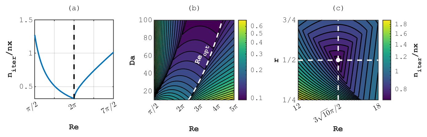
Figure 1Number of iterations per grid point required for e-fold residual reduction. Panels (a), (b) and (c) correspond to stationary diffusion, stationary diffusion–reaction and incompressible 2D Stokes problems, respectively.
We present detailed explanations and derivations of the dispersion analysis of different problems in the Appendix A, leading to the optimal value of Re:
We quantify the convergence rate by the number of iterations niter required to reduce the maximal deviation of the solution to the PT equation from the true solution to the corresponding stationary problem by a factor of e (base of natural logarithm), divided by the number of grid cells nx. Results of the dispersion analysis for the 1D stationary diffusion problem show niter≈0.3nx given optimal values of Re (Fig. 1a). We estimate that the residual reduction by 14 orders of magnitude requires only ∼10nx iterations.
For simplicity we only consider the case D=const in the dispersion analysis. In this case, both and θr are constant. If the physical properties vary in space, i.e. D=D(xk), the iteration parameters and θr are no longer constant and must be locally defined by the value corresponding to each grid point. If the distribution of D is smooth, this approximation works well in practice, and the number of iterations is close to the theoretically predicted value. However, particular care is needed when the distribution of D is discontinuous in space to avoid significantly reduced values of to be required for convergence, ultimately leading to a much higher number of PT iterations. We found that taking a local maximum of D between neighbouring grid cells in the definitions of iteration parameters, Eqs. (9) and (10), is sufficient to ensure optimal convergence. The per-grid point local maximum selection thus effectively acts as a preconditioning technique.
For nonlinear and/or complex flow problems, the corresponding optimal values of iteration parameters such as numerical Reynolds number Re may be determined by systematic numerical experiments. In practice, optimal values for iteration parameters do not differ significantly from theoretical predictions derived for the linear case (see Sect. 2.1.3). Most importantly, the linear scaling of the method is still preserved. Also, the accelerated PT method admits explicit numerical integration, and can be implemented with minimal modifications of the simplest PT method.
2.1.3 Diffusion–reaction
The next example addresses stationary diffusion processes coupled with reaction. Here, we assume that reaction is described by the first-order kinetics law:
where Heq is the value of H at equilibrium, and θk is a characteristic time of reaction. The flux q in Eq. (12) is governed by either Eq. (2) or (6). The addition of a source term does not change the type of PDE involved in the method formulation, and the iteration strategy based on the discretisation of Eq. (2) still exhibits a quadratic scaling. We therefore focus only on the analysis of the accelerated PT method.
Equations (12) and (6) reduce to the following equation governing the evolution of H:
The Eq. (13) differs from the damped wave equation (Eq. 7) in that it includes the source term and additional physical parameters θk and ρ. In the non-dimensional form, all parameters of Eq. (13) can be reduced to two non-dimensional numbers: Re, defined equivalently to the stationary diffusion case, and , a new parameter, which can be interpreted as a Damköhler number characterising the ratio of characteristic diffusion time to reaction timescale. Contrary to the numerical parameter Re, Da depends only on the physical parameters and cannot be arbitrarily specified.
We present the detailed dispersion analysis for the stationary diffusion–reaction problem in Sect. A3 of the Appendix. Parameters and θr are defined according to Eqs. (9) and (10), respectively, and by analogy to the stationary diffusion case. Optimal values of Re now depend on the parameter Da:
We report the result of the dispersion analysis for the diffusion–reaction case as the number of iterations required for an e-fold residual reduction niter per grid point nx as a function of Re and Da, highlighting Reopt as a function of Da by a dashed line (Fig. 1b). In the limit Da→0, i.e. when the characteristic time of reaction is infinitely large compared to the characteristic time of diffusion, Reopt→2π, which is the optimal value for the stationary diffusion problem discussed in Sect. 2.1.2. In that limit, the number of iterations required for an e-fold residual reduction niter is also equivalent to the stationary diffusion problem. However, as Da increases, the process becomes progressively more reaction-dominated and the PT iterations converge accordingly faster.
2.1.4 Transient diffusion
It is possible to apply the PT method not only to the solution of stationary problems, but also to problems including physical transient terms. This method is known in the literature as the “dual-time”, or “dual time stepping” method (Gaitonde, 1998; Mandal et al., 2011).
According to the dual-time method, both physical and pseudo-time derivatives are present in the equation:
The discretisation of the physical time derivative in Eq. (15) using a first-order backward Euler scheme, leads to
where is the distribution of H at the explicit layer of the integration scheme, and Δt is the physical time step. Comparing Eqs. (16) and (12) shows the two equations to be mathematically identical. Therefore, the optimal iteration parameters given by Eq. (A15) apply to the transient diffusion as well. The Da parameter thus equals and characterises the fraction of the domain traversed by a particle transported by a diffusive flux during time Δt. The optimal value of Re is then defined as
Frequently, modelling of certain processes requires relatively small time steps in order to capture important physical features, e.g. shear-heating induced strain localisation (Duretz et al., 2019a) or spontaneous flow localisation in porous media (Räss et al., 2019a). In such cases, values of Da can be very large. Also, every step of numerical simulation serves as a good initial approximation to the next simulation step, thereby reducing error amplitude E1 in Eq. (A16).
2.2 Incompressible viscous shear-driven Couette flow
Before considering incompressible Stokes equations, we present an illustrative example of shear-driven flow to demonstrate a similarity between already discussed cases addressing generalised diffusion and viscous fluid flow.
Here we consider stationary fluid flow between two parallel plates separated by a distance L. We assume the absence of pressure gradients in directions parallel to the plates. In that case, Stokes equations are reduced to the following system:
where τxi is the deviatoric shear stress, vx is the velocity parallel to the plates, and μs is the shear viscosity.
The steady-state process described by Eqs. (18) and (19) can be converted to a PT process similar to the one presented in Sect. 2.1.2, by considering the inertial term in the momentum equation (Eq. 18) and Maxwell visco-elastic rheology as a constitutive relation for the viscous fluid Eq. (19):
Here, and are numerical parameters, interpreted as density and elastic shear modulus, respectively. The system of equations (Eqs. 20 and 21) is mathematically equivalent to the system of equations (Eqs. 1 and 6), describing PT diffusion of the velocity field vx. The relaxation time θr in that case represents the Maxwell relaxation time, and is equal to .
2.3 Incompressible viscous Stokes equation
The next example addresses the incompressible creeping flow of a viscous fluid, described by Stokes equations:
where τij is the deviatoric stress, p is the pressure, δij is the Kronecker delta, fi is the body forces, v is the velocity, and is the deviatoric strain rate.
Similar to the shear-driven flow described in Sect. 2.2, a solution to the system (Eqs. 22–24) can be achieved by PT time integration described by
Equations (25) and (26) now both include pseudo-time derivatives of velocity and pressure, and become an inertial and acoustic approximation to the momentum and mass balance equations, respectively. The additional parameter arising in Eq. (26) can be interpreted as a numerical or pseudo-bulk modulus.
We use the primary, or P-wave velocity, as a characteristic velocity scale for the Stokes problem:
In addition to the non-dimensional numerical Reynolds number, here defined as , we introduce the ratio between the bulk and shear elastic modulus .
By analogy to previous cases, substituting and solving the numerical parameters , and yields
Similar to the diffusion–reaction problem studied in Sect. 2.1.3, there are two numerical parameters controlling the process. However, in Stokes equations, both parameters are purely numerical and could be tuned to achieve the optimal convergence rate.
The dispersion analysis for 1D linear Stokes equations is detailed in Sect. A4 of the Appendix. We provide the resulting optimal values to converge the 2D Stokes problem:
because they differ from the 1D case values, and because we consider 2D and 3D Stokes formulation in the remaining of this study.
In the numerical experiments, we consistently observe faster convergence with slightly higher values of r≈1, likely caused by the fact that some of the assumptions made for 1D dispersion analysis do not transfer to the 2D formulation (Fig. 1c). Thus, the values presented in Eqs. (31)–(32) should only be regarded as an estimate of optimal iteration parameters.
2.4 Incompressible visco-elastic Stokes equation
The last example addresses the incompressible Stokes equations accounting for a physical visco-elastic Maxwell rheology:
where G is the physical shear modulus.
As in the transient diffusion case presented in Sect. 2.1.4, the problem can be augmented by PT time integration using a dual time stepping approach:
Collecting terms in front of τij and ignoring because it does not change between successive PT iterations, one can reduce the visco-elastic Stokes problem to the previously discussed viscous Stokes problem by replacing the viscosity in the Eq. (28) with the effective “visco-elastic” viscosity:
The conclusions and optimal parameters' values presented in Sect. 2.3 thus remain valid for the visco-elastic rheology as well.
Assessing the performance of iterative stencil-based applications is 2-fold and reported here in terms of algorithmic and implementation efficiency.
The accelerated PT method provides an iterative approach that ensures linear scaling of the iteration count with an increase in numerical grid resolution nx (Sect. 2) – the algorithmic scalability or performance. The major advantage in the design of such an iterative approach is its concise implementation, extremely similar to explicit time integration schemes. Explicit stencil-based applications, such as elastic wave propagation, can show optimal performance and scaling on multi-GPU configurations because they can keep memory access to the strict minimum, leverage data locality and only require point-to-point communication (Podladtchikov and Podladchikov, 2013). Here we follow a similar strategy.
We introduce two metrics: the effective memory throughput (Teff) and the parallel efficiency (E) (Kumar et al., 1994; Gustafson, 1988; Eager et al., 1989). Early formulations of effective memory throughput analysis are found in Omlin et al. (2015a, b); Omlin (2017). The effective memory throughput permits the assessment of the single-processor (GPU or CPU) performance and allows us to deduce potential room for improvement. The parallel efficiency permits the assessment of distributed-memory scalability which may be hindered by interprocess communication, congestion of shared file systems and other practical considerations from scaling on large supercomputers. We perform single-GPU problem size scaling benchmarks to assess the optimal local problem size based on the Teff metric. We further use the optimal local problem size in weak-scaling benchmarks to assess the parallel efficiency E(N,P).
3.1 The effective memory throughput
Many-core processors such as GPUs are throughput-oriented systems that use their massive parallelism to hide latency. On the scientific application side, most algorithms require fewer floating-point operations per second (FLOPS), compared to the amount of numbers or bytes accessed from main memory, and thus are significantly memory bound. The FLOPS metric, no longer being the most adequate for reporting the application performance (e.g. Fuhrer et al., 2018) in a majority of cases, motivated us to develop a memory throughput-based performance evaluation metric, Teff, to evaluate the performance of iterative stencil-based PDE solvers.
The effective memory access, Aeff [GB], is the sum of twice the memory footprint of the unknown fields, Du, (fields that depend on their own history and that need to be read from and written to every iteration) and the known fields, Dk, that do not change every iteration. The effective memory access divided by the execution time per iteration, tit [s], defines the effective memory throughput, Teff [GB s−1]:
The upper bound of Teff is Tpeak as measured e.g. by McCalpin (1995) for CPUs or a GPU analogue. Defining the Teff metric, we assume that (i) we evaluate an iterative stencil-based solver, (ii) the problem size is much larger than the cache sizes and (iii) the usage of time blocking is not feasible or advantageous (which is a reasonable assumption for real-world applications). An important concept is to not include fields within the effective memory access that do not depend on their own history (e.g. fluxes); such fields can be recomputed on the fly or stored on-chip. Defining a theoretical upper bound for Teff that is closer to the real upper bound is a work in progress (Omlin and Räss, 2021b).
3.2 The parallel efficiency
We employ the parallel efficiency metric to assess the scalability of the iterative solvers when targeting distributed-memory configurations, such as multi-GPU settings. In a weak-scaling configuration, i.e. where the global problem size and computing resources increase proportionally, the parallel efficiency E(N,P) defines the ratio between the execution time of a single process, T(N,1), and the execution time of P processes performing the same number of iterations on a P-fold larger problem, , where N is the local problem size and P is the number of parallel processes:
Distributed parallelisation permits overcoming limitations imposed by the available main memory of a GPU or CPU. It is particularly relevant for GPUs, which have significantly less main memory available than CPUs. Distributing work amongst multiple GPUs, using e.g. the message passing interface (MPI), permits overcoming these limitations and requires parallel computing and supercomputing techniques. Parallel efficiency is a key metric in light of assessing the overall application performance as it ultimately ensures scalability of the PT method.
We design a suite of numerical experiments to verify the scalability of the accelerated PT method, targeting diffusive processes and mechanics. We consider three distinct diffusion problems in one, two and three dimensions, that exhibit a diffusion coefficient being (i) linear, (ii) a step function with 4 orders of magnitude contrasts and (iii) a cubic power-law relation. We then consider mechanical processes using a velocity–pressure formulation to explore various limits, including variable-viscosity incompressible viscous flow limit, accounting for a Maxwell visco-elastic shear rheology. To demonstrate the versatility of the approach, we tackle the nonlinear mechanical problem of strain localisation in two and three dimensions considering an E-VP rheology (Sect. 8). We verify the robustness of the accelerated PT method by considering two parametric studies featuring different viscous Stokes flow patterns, and demonstrate the convergence of the method for viscosity contrasts up to 9 orders of magnitude. We finally investigate the convergence of visco-elastic Stokes flow for non-similar domain aspect ratio.
4.1 Diffusive processes
We first consider time-dependent (transient) diffusion processes defined by Eqs. (1) and (2), with the proportionality coefficient ρ=1. Practical applications often exhibit at least one diffusive component which can be either linear or nonlinear. Here, we consider linear and nonlinear cases representative of challenging configurations common to a broad variety of forward numerical diffusion-type models:
-
The first case exhibits a linear constant (scalar) diffusion coefficient:
-
The second case exhibits a spatially variable diffusion coefficient with a contrast of 4 orders of magnitude:
where L is the domain extent in a specific dimension and LD the coordinate at which the transition occurs. Large contrasts in material parameters (e.g. permeability or heat conductivity) are common challenges that solvers needs to handle when targeting real-world applications.
-
The third case exhibits a nonlinear power-law diffusion coefficient:
where n=3, is a characteristic value in, e.g. soil and poro-mechanical applications to account for the porosity–permeability Carman–Kozeny (Costa, 2006) relation leading to the formation of solitary waves of porosity. Shallow ice approximation or nonlinear viscosity in power-law creep Stokes flow are other applications that exhibit effective diffusion coefficients to be defined as power-law relations.
Practically, we implement the transient diffusion using the accelerated PT method, solving Eqs. (6) and (15) using a dual-time method (Sect. 2.1.4).
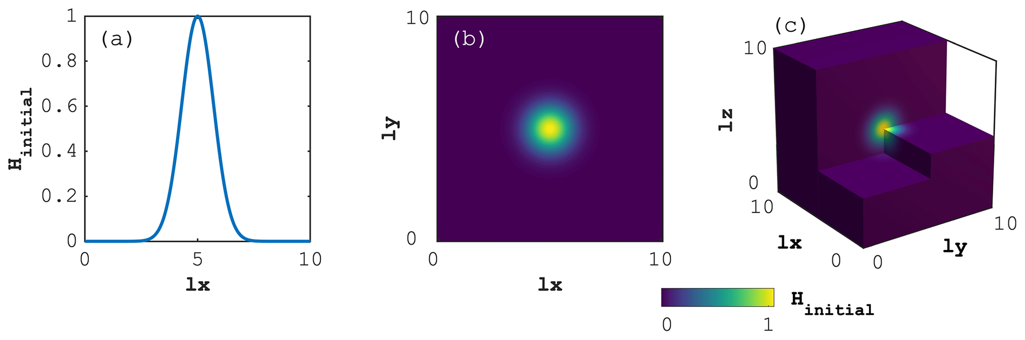
Figure 2Initial distribution of H for the (a) 1D, (b) 2D and (c) 3D time-dependent diffusion configurations.
4.2 Mechanics
We secondly consider steady-state mechanical problems, defined by Eqs. (22) and (23). In practice, we employ a velocity–pressure formulation, which allows us to also handle the incompressible flow limit. The rheological model builds on an additive decomposition of the deviatoric strain rate tensor (Maxwell's model), given by Eq. (33).
In Sect. 5.2, the mechanical problem is solved in the incompressible limit and assuming a linear visco-elastic deviatoric rheology.
In the subsequent application (Sect. 8), the mechanical problem is solved in the compressible E-VP limit. Hence, the deviatoric rheological model neglects viscous flow and includes viscoplastic flow:
where and Q stand for the rate of the plastic multiplier and the plastic flow potential, respectively. A similar decomposition is assumed for the divergence of velocity in Eq. (23), which is no longer equal to zero in order to account for elastic and plastic bulk deformation:
where K stands for the physical bulk modulus.
In the inclusion parametric study described in Sect. 5.2, we consider the incompressible viscous Stokes flow limit, i.e. K→∞ and G→∞.
5.1 The diffusion model
We perform the three different diffusion experiments (see Sect. 4.1) on 1D, 2D and 3D computational domains (Fig. 2a, b and c, respectively). The only difference between the numerical experiments lies in the definition of the diffusion coefficient D. The non-dimensional computational domains are , and , for 1D, 2D and 3D domains, respectively. The domain extent is . The initial condition, H0, consists of a Gaussian distribution of amplitude and standard deviation equal to one located in the domain's centre; in the 1D case:
where xc is the vector containing the discrete 1D coordinates of the cell centres. The 2D and 3D cases are done by analogy and contain the respective terms for the y and z directions. We impose Dirichlet boundary conditions such that H=0 on all boundaries. We simulate a total non-dimensional physical time of 1 performing five implicit time steps of Δt=0.2.
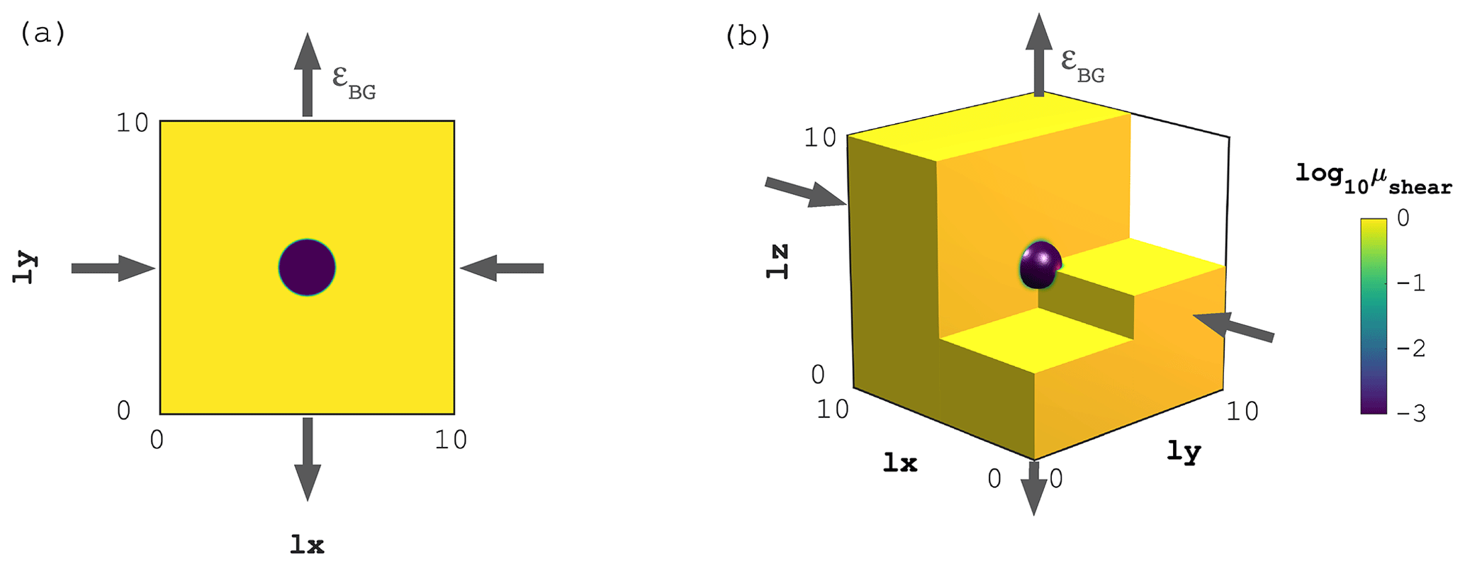
Figure 3Initial shear viscosity (μshear) distribution for the (a) 2D and (b) 3D visco-elastic Stokes flow configuration, respectively.
5.2 The Stokes flow model
We perform the visco-elastic Stokes flow experiments (see Sect. 4.2) on 2D and 3D computational domains (Fig. 3a and b, respectively). The non-dimensional computational domains are and for 2D and 3D domains, respectively. The domain extend is . As an initial condition, we define a circular (2D) or spherical (3D) inclusion of radius r=1 centred at (2D) and (3D), featuring 3 orders of magnitude with lower shear viscosity compared to the background value (Fig. 3). We then perform 10 explicit diffusion steps of the viscosity field μs to account for smoothing introduced by commonly employed advection schemes (e.g. markers-in-cell, semi-Lagrangian or weighted ENO). We define a uniform and constant elastic shear modulus G=1 and chose the physical time step to satisfy a visco-elastic Maxwell relaxation time of ξ=1. We impose pure shear boundary conditions; we apply compression in the x direction and extension in the vertical (y in 2D, z in 3D) direction with a background strain rate εBG=1. For the 3D case, we apply no inflow/outflow in the y direction (Fig. 3b). All model boundaries are free to slip. We perform a total of five implicit time steps to resolve visco-elastic stress build-up.
We further perform a series of viscous Stokes numerical experiments in 2D (see Sect. 4.2) to analyse the dependence of the optimal iteration parameters on the material viscosity contrast and the volume fraction of the material with lower viscosity. The non-dimensional computational domain is . As an initial condition, we define a number ninc of circular inclusions that are semi-uniformly distributed in the domain. The viscosity in the inclusions is and the background viscosity is .
In the parametric study, we vary the number of inclusions ninc, the inclusion viscosity , and the iteration parameter Re. We consider a uniform 3D grid of parameter values, numerically calculating the steady-state distribution of stresses and velocities for each of these combinations.
We consider two different problem setups that correspond to important edge cases. The first setup addresses the shear-driven flow where the strain rates are assumed to be applied externally via boundary conditions. This benchmark might serve as a basis for the calculation of effective-media properties. The second setup addresses the gravity-driven flow with buoyant inclusions. This benchmark is relevant for geophysical applications, e.g. modelling magmatic diapirism or melt segregation, where the volumetric effect of melting leads to the development of either the Rayleigh–Taylor instability or compaction instability, respectively.
In the first setup, we specify pure-shear boundary conditions similar to the singular inclusion case described in Sect. 5.2. The body forces fi are set to zero in Eq. (22).
In the second setup, we specify the free-slip boundary conditions, which correspond to setting the background strain rate εBG to 0. We model buoyancy using the Boussinesq approximation: the density differences are accounted for only in the body forces. We set fx=0, . We set ρg0=1, ρginc=0.5.
We discretise the systems of partial differential equations (Sect. 4) using the finite-difference method on a regular Cartesian staggered grid. For the diffusion process, the quantity being diffused and the fluxes are located at cell centres and cell interfaces, respectively. For the Stokes flow, pressure, normal stresses and material properties (e.g. viscosity) are located at cell centres, while velocities are located at cell interfaces. Shear stress components are located at cell vertices. The staggering relies on second-order conservative finite differences (Patankar, 1980; Virieux, 1986; McKee et al., 2008), also ensuring that the Stokes flow is inherently devoid of oscillatory pressure modes (Shin and Strikwerda, 1997).
The diffusion process and the visco-elastic Stokes flow include physical time evolution. We implement a backward Euler time integration within the PT solving procedure (see Sect. 2) and do not assess higher-order schemes as such considerations go beyond the scope of this study.
In all simulations we converge the scaled and normalised L2-norm of the residuals, , where nR stands for the number of entries of R, for each physical time step to a nonlinear absolute tolerance of within the iterative PT procedure (absolute and relative tolerances being comparable, given the non-dimensional form of the example we consider here).
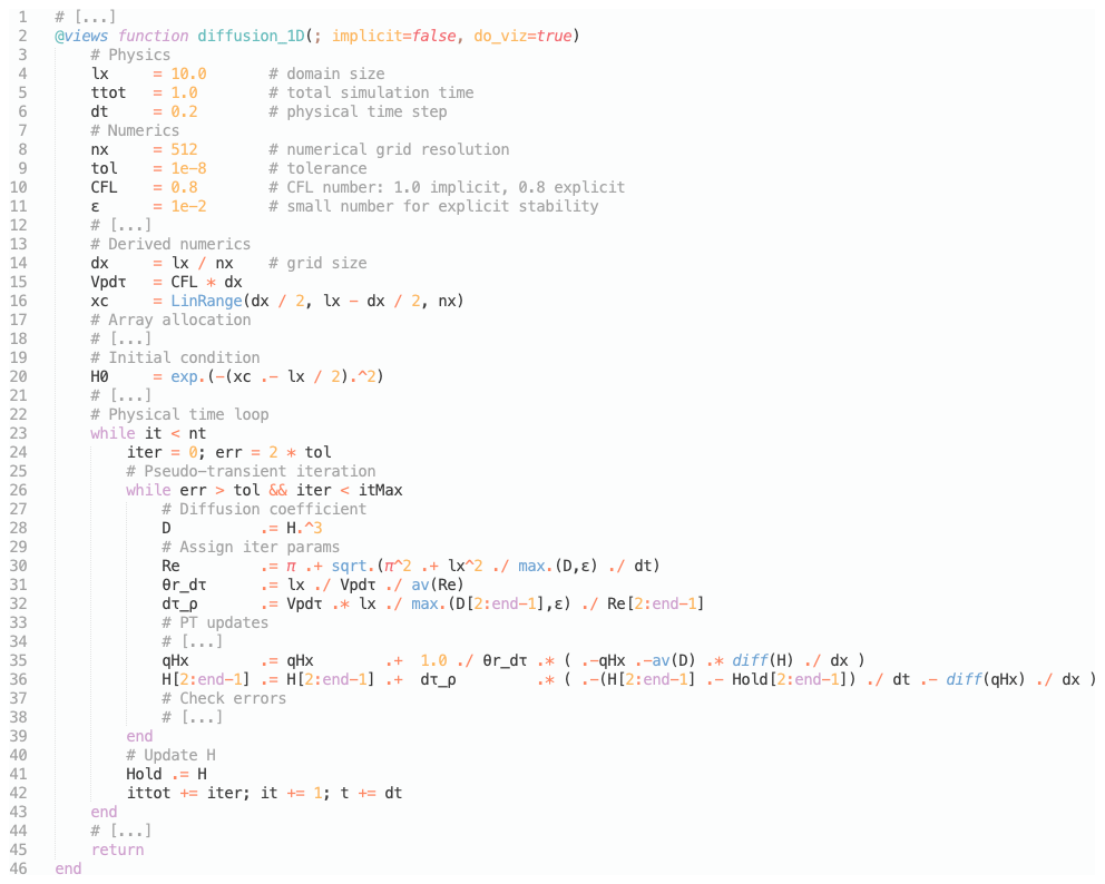
Figure 4Numerical Julia implementation of the 1D nonlinear diffusion case D=H3. Lines marked with # [...] refer to skipped lines. See diff_1D_nonlin_simple.jl script located in the scripts folder in PseudoTransientDiffusion.jl on GitHub for full code.
The 46-line code fragment (Fig. 4) provides information about the concise implementation of the accelerated PT algorithm, here for the 1D nonlinear power-law diffusion case (D=H3). Besides the initialisation part (lines 3–22), the core of the algorithm is contained in no more than 20 lines (lines 23–43). The algorithm is implemented as two nested (pseudo-)time loops, referred to as “dual-time”; the outer loop advancing in physical time, the inner loop converging the implicit solution in pseudo-time. The nonlinear term, here the diffusion coefficient D, is explicitly evaluated within the single inner-loop iterative procedure, removing the need for performing nonlinear iterations on top of a linear solver (e.g. Brandt, 1977; Trottenberg et al., 2001; Hackbusch, 1985). This single inner-loop local linearisation shows, in practice, a lower iteration count when compared to global linearisation (nested loops). Note that a relaxation of nonlinearities can be implemented in a straightforward fashion if the nonlinear term hinders convergence (see implementation details in e.g. Räss et al., 2020, 2019a; Duretz et al., 2019b). The iteration parameters are evaluated locally which ensures scalability of the approach and removes the need for performing global reductions, costly in parallel implementation. Note that the numerical iteration parameters and θr, arising from the finite-difference discretisation of pseudo-time derivatives in Eqs. (16) and (6),
where k is the current pseudo-time iteration index, always occur in combination with Δτ. Since we are not interested in the evolution of pseudo-time or the particular values of iteration parameters, it is possible to combine them in the implementation. We therefore introduce the variables and . Using the new variables helps to avoid specifying the value of Δτ, which could otherwise be specified arbitrarily.
The two lines of physics, namely the PT updates, are here evaluated in an explicit fashion. Alternatively, one could solve qHx and H assuming that their values in the residual – the terms contained in the right-most parenthesis – are new instead of current, resulting in an implicit update. Advantages rely on enhanced stability (CFL on line 10 could be set to 1) and remove the need for defining a small number (ε in the iteration parameters definition) to prevent division by 0. The implicit approach is implemented as an alternative in the full code available online in the PseudoTransientDiffusion.jl GitHub repository.
6.1 The Julia multi-xPU implementation
We use the Julia language (Bezanson et al., 2017) to implement the suite of numerical experiments. Julia's high-level abstractions, multiple dispatch and meta-programming capabilities make it amenable to portability between back-ends (e.g. multi-core CPUs and Nvidia or AMD GPUs). Also, Julia solves the two-language problem, making it possible to fuse prototype and production applications into a single one that is both high-level and performance oriented – ultimately increasing productivity.
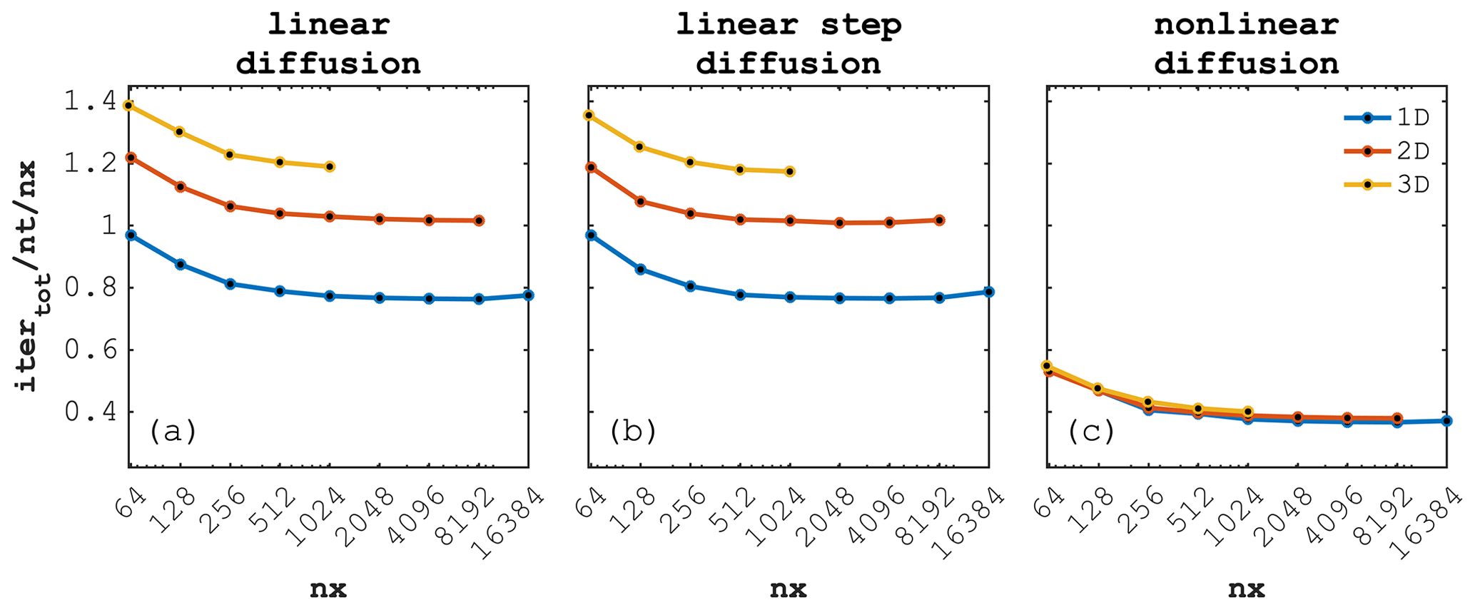
Figure 5Iteration count scaled by the number of time steps (nt) and by the number of grid cells in the x direction (nx) as function of nx, comparing 1D, 2D and 3D models for the three different diffusion configurations: (a) linear diffusion, (b) linear step diffusion and (c) nonlinear diffusion, respectively.
We use the ParallelStencil.jl (Omlin and Räss, 2021b) and ImplicitGlobalGrid.jl (Omlin and Räss, 2021a) Julia packages that we developed as building blocks to implement the diffusion and Stokes numerical experiments. ParallelStencil.jl permits to write architecture–agnostic high-level code for parallel high-performance stencil computations on GPUs and CPUs – here referred to as xPUs. Performance similar to native CUDA C/C++ (Nvidia GPUs) or HIP (AMD GPUs) can be achieved. ParallelStencil.jl seamlessly combines with ImplicitGlobalGrid.jl, which allows for distributed parallelisation of stencil-based xPU applications on a regular staggered grid. In addition, ParallelStencil.jl enables hiding communication behind computation, where the communication package used can, a priori, be any package that allows the user to control when communication is triggered. The overlap approach of communication and computation splits local domain calculations into two regions, i.e. boundary regions and inner region, the latter containing majority of the local domain's grid cells. After successful completion of the boundary region computations, halo update (using e.g. point-to-point MPI) overlaps with inner-point computations. Selecting the appropriate width of the boundary region permits fine-tuning the optimal hiding of MPI communication (Räss et al., 2019c; Alkhimenkov et al., 2021b).
In the present study, we focus on using ParallelStencil.jl with the CUDA.jl back-end to target Nvidia GPUs (Besard et al., 2018, 2019), and ImplicitGlobalGrid.jl which relies on MPI.jl (Byrne et al., 2021) and Julia's MPI wrappers to enable distributed-memory parallelisation.
We here report the performance of the accelerated PT Julia implementation of the diffusion and the Stokes flow solvers targeting Nvidia GPUs using ParallelStencil.jl's CUDA back-end. For both physical processes, we analyse the iteration count as a function of the number of grid cells (i.e. the algorithmic performance), the effective memory throughput Teff [GB s−1] (performing a single-GPU device problem size scaling), and the parallel efficiency E (multi-GPU weak scaling).
We report the algorithmic performance as the iteration count per number of physical time steps normalised by the number of grid cells in the x direction. We do not normalise by the total number of grid cells in order to report the 1D scaling, even for 2D or 3D implementation. We motivate our choice as it permits a more accurate comparison to analytically derived results and leaves it to the reader to appreciate the actual quadratic and cubic dependence of the normalised iteration count if using the total number of grid cells in 2D and 3D configurations, respectively.
7.1 Solving the diffusion equation
We report a normalised iteration count per total number of physical time steps nt per number of grid cells in the x direction nx ( ), for the 1D, 2D and 3D implementations of the diffusion solver for the linear, step-function and nonlinear case (Fig. 5a, b and c, respectively) relating to the spatial distribution of H after 5 implicit time steps (Fig. 6a–c, d–f and g–i, respectively). All three different configurations exhibit a normalised number of iterations per time step per number of grid cells close to 1 for the lowest resolution of nx=64 grid cells. The normalised iteration count drops with an increase in numerical resolution (increase in number of grid cells) suggesting a super-linear scaling.
We observe similar behaviour when increasing the number of spatial dimensions while solving the identical problem. For example, in the 3D calculations we actually resolve (here ) grid cells, while the reported nx-normalised iteration count only slightly increases compared to the corresponding 1D case.
It is interesting to note that the diffusion solver with nonlinear (power-law) diffusion coefficient reports the lowest normalised iteration count for all three spatial dimension implementations, reaching the lowest number (>0.4) of normalised iteration count in the 3D configuration (Fig. 5c). The possible explanation of lower iteration counts for the nonlinear problem is that by the nature of the solution, the distribution of the diffused quantity H at t=1 is much closer to the initial profile than in the linear case. Therefore, at each time step, the values of H are closer to the values of H at the next time step and thus serve as a better initial approximation. Both the diffusion with linear (Fig. 5a) and step function as diffusion coefficient (Fig. 5b) show similar trends in their normalised iteration counts, with values decreasing while increasing the number of spatial dimensions.
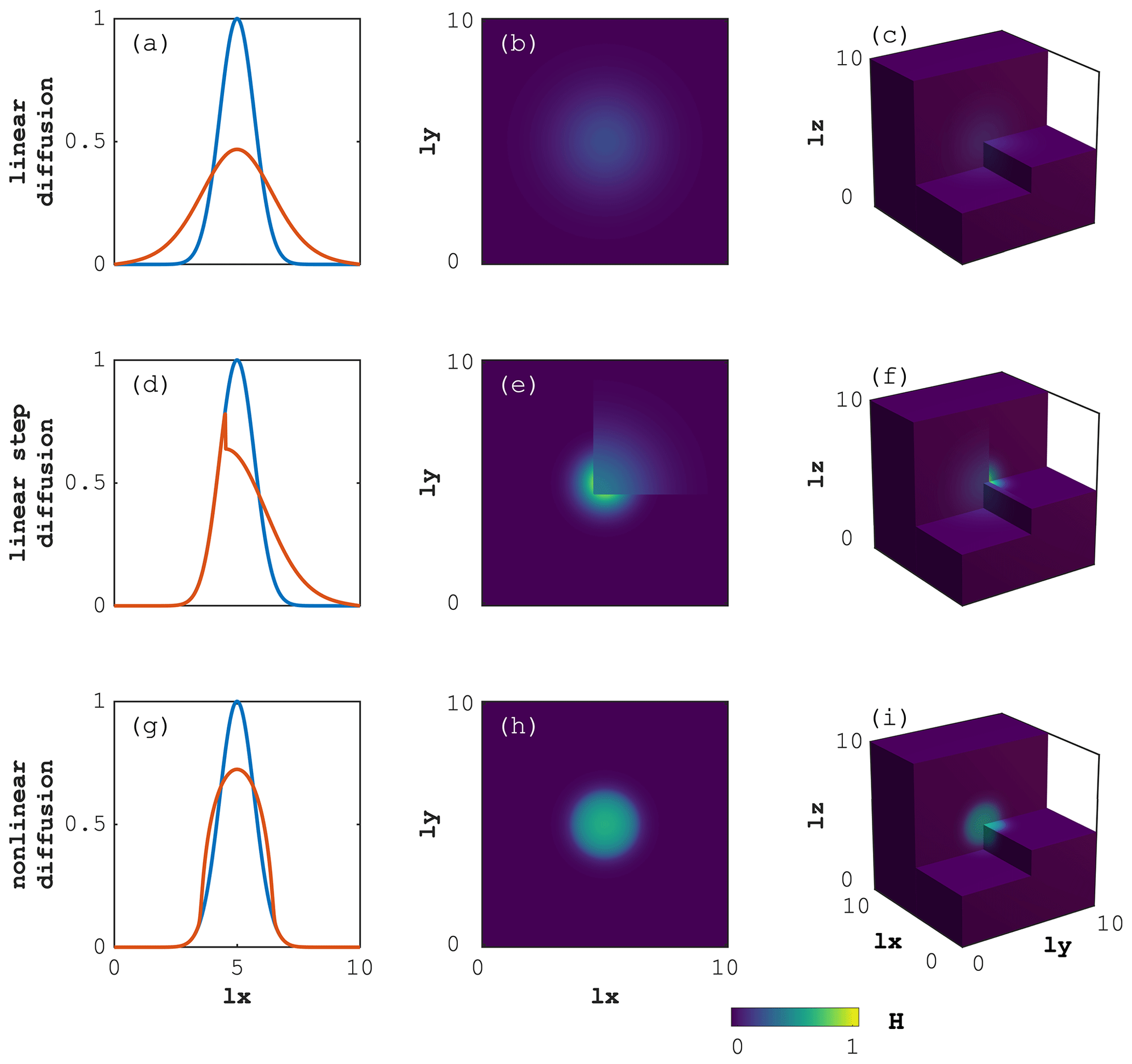
Figure 6Model output for the 1D (a, d, g), 2D (b, e, h) and 3D (c, f, i) time-dependent diffusion of quantity H. The upper (a–c), centre (d–f) and lower (g–i) panels refer to the diffusion with linear, linear step and nonlinear (power-law) diffusion coefficient, respectively. For the 1D case, the blue and red lines represent the initial and final distribution, respectively. The colour map (2D and 3D) relates to the y axis (1D).
7.2 Solving visco-elastic Stokes flow
We further report the normalised iteration count per total number of physical time steps nt per number of grid cells in the x direction nx () for the 2D and 3D implementations of the visco-elastic Stokes solver (Fig. 7) relating to the spatial distribution of vertical velocity (deviation from background) ΔVvertical, pressure P and shear stress τshear after 5 implicit time steps (Fig. 8a–b, c–d and e–f, respectively). Both 2D and 3D visco-elastic Stokes flow exhibit a normalised number of iterations per time step per number of grid cells close to 10 for the lowest resolution of nx=63 grid cells. The normalised iteration count drops with an increase in numerical resolution (increase in number of grid cells) suggesting a super-linear scaling. We observe similar behaviour when increasing the number of spatial dimensions from 2D to 3D, while solving the identical problem; 3D calculations are more efficient on a given number of grid cells nx compared to the corresponding 2D calculations, which is in accordance with results for the various diffusion solver configurations.
The visco-elastic Stokes flow scaling results confirm the trend reporting a decrease of the normalised iteration count with an increase in the numerical resolution (number of grid cells). It is interesting to note that the accelerated PT implementation of the 3D visco-elastic Stokes flow featuring 3 orders of magnitude viscosity contrast () only requires less than 17 normalised iterations when targeting resolutions of 10233 (Fig. 7).
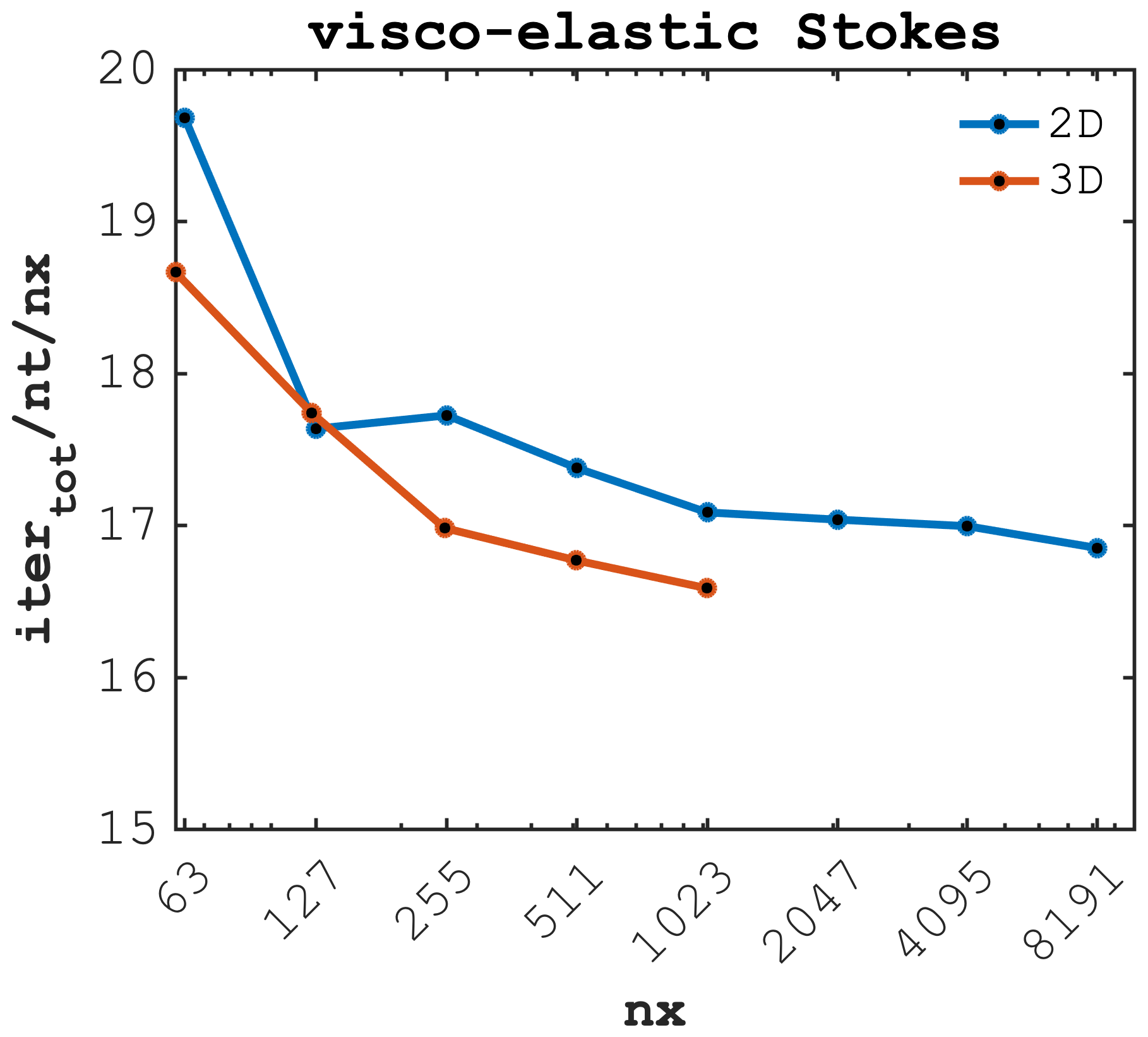
Figure 7Iteration count scaled by the number of time steps (nt) and by the number of grid cells in the x direction (nx) as function of nx, comparing 2D and 3D visco-elastic Stokes flow containing an inclusion featuring a viscosity contrast ().

Figure 8Model output for the 2D (a, c, e) and 3D (b, d, f) visco-elastic Stokes flow containing an inclusion featuring a viscosity contrast (). The upper (a–b), centre (c–d), and lower (e–f) panels depict the deviation from background vertical velocity ΔVvertical, the dynamic pressure P and deviatoric shear stress τshear(τxy in 2D, τxz in 3D) distribution, respectively.
7.3 Performance
We use the effective memory throughput Teff [GB s−1] and the parallel efficiency E(N,P) to assess the implementation performance of the accelerated PT solvers, as motivated in Sect. 3. We perform the single-GPU problem size scaling and the multi-GPU weak-scaling tests on different Nvidia GPU architectures, namely the “data-centre” GPUs, Tesla P100 (Pascal – PCIe), Tesla V100 (Volta – SXM2) and Tesla A100 (Ampere – SXM4). We run the weak-scaling multi-GPU benchmarks on the Piz Daint supercomputer, featuring up to 5704 Nvidia Tesla P100 GPUs, at CSCS, on the Volta node of the Octopus supercomputer, featuring 8 Nvidia Tesla V100 GPUs with high-throughput (300 GB s−1) SXM2 interconnect, at the Swiss Geocomputing Centre, University of Lausanne, and on the Superzack node, featuring 8 Nvidia Tesla A100 GPUs with high-throughput (600 GB s−1) SXM4 interconnect, at the Laboratory of Hydraulics, Hydrology, Glaciology (VAW), ETH Zurich.
We assess the performance of the 2D and 3D implementations of the nonlinear diffusion solver (power-law diffusion coefficient) and the visco-elastic Stokes flow solver, respectively. We perform single-GPU scaling tests for both the 2D and 3D solvers' implementation, and multi-GPU weak-scaling tests for the 3D solvers' implementation only. We report the mean performance out of 5 executions, if applicable.
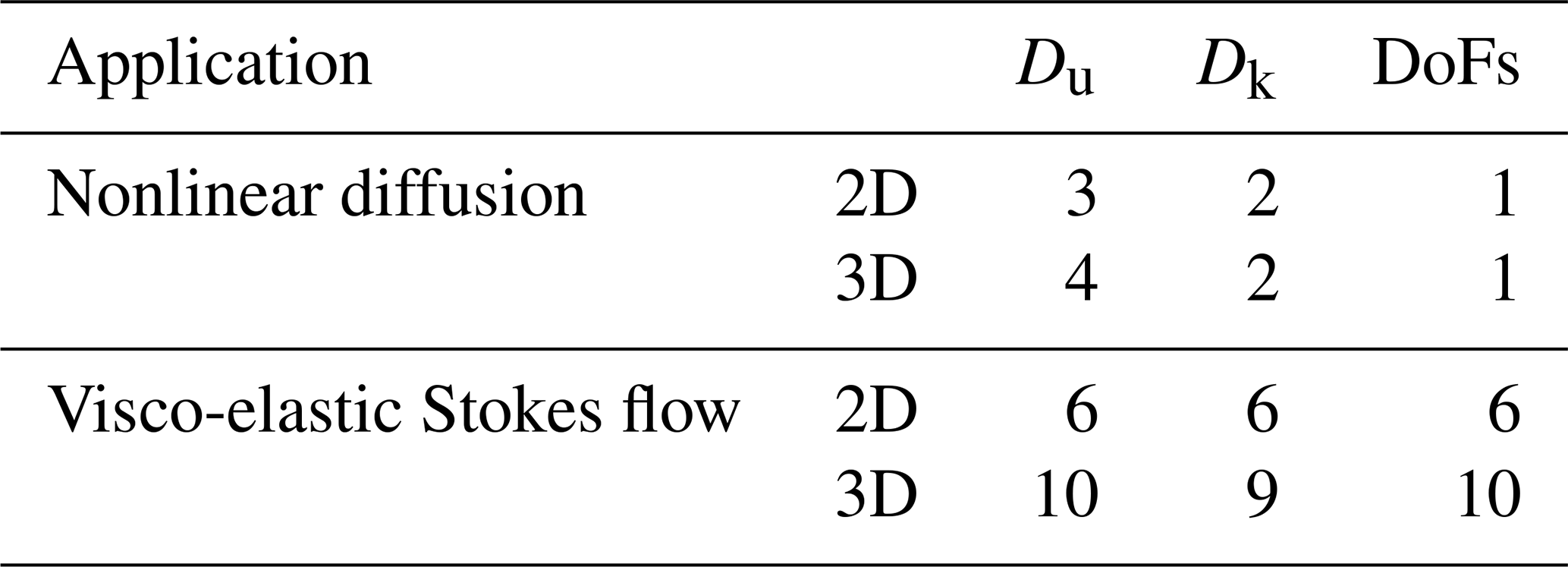
In order to compute the effective memory throughput Teff in the scaling test, we need to determine the number of unknown and known fields the solvers access during the iterative procedures (see Sect. 3.1). We report the values we use for the nonlinear diffusion solver and the visco-elastic Stokes flow solver in both 2D and 3D, as well as the per grid cell number of DoFs in Table 1.
Table 1Number of unknown (Du) and known (Dk) fields, as well as per grid cell DoFs used to assess, e.g. the Teff metric in the performance scaling tests.
7.3.1 Single-GPU scaling and effective memory throughput
The 2D and 3D nonlinear diffusion solver single-GPU scaling benchmarks achieve similar effective memory throughput on the targeted GPU architectures relative to their respective peak values Tpeak; values of Teff for the 2D implementation being slightly higher than the 3D ones for the Volta and Pascal architectures, but similar for the Ampere one. This discrepancy is expected and may be partly explained by an increase in cache-misses when accessing z-direction neighbours which are nx⋅ny grid cells away in main memory. In 2D, we achieve Teff≈920, 590 and 400 GB s−1 on the Tesla A100, Tesla V100 and the Tesla P100, respectively (Fig. 9a). In 3D, we achieve Teff≈920, 520 and 315 GB s−1 on the Tesla A100, Tesla V100 and the Tesla P100, respectively (Fig. 9b).
For the analogous visco-elastic Stokes flow single-GPU scaling tests, we also report higher Teff values for the 2D compared to the 3D implementation for all three targeted architectures. In 2D, we achieve Teff≈930, 500 and 320 GB s−1 on the Tesla A100, Tesla V100 and the Tesla P100, respectively (Fig. 10a). In 3D, we achieve Teff≈730, 350 and 230 GB s−1 on the Tesla A100, Tesla V100 and the Tesla P100, respectively (Fig. 10b). Increased neighbouring access and overall more derivative evaluations may explain the slightly lower effective memory throughput of the visco-elastic Stokes flow solver when compared to the nonlinear diffusion solver.
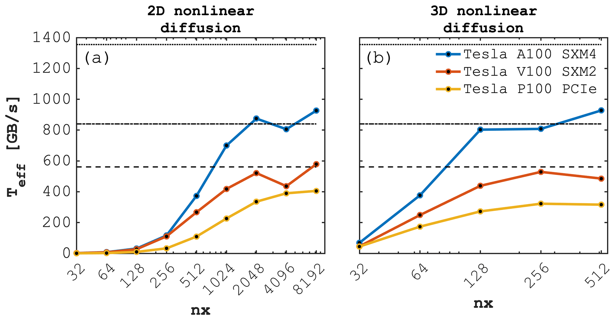
Figure 9Effective memory throughput Teff [GB s−1] for the (a) 2D and (b) 3D nonlinear diffusion Julia GPU implementations using ParallelStencil.jl executed on various Nvidia GPUs (Tesla A100 SXM4, Tesla V100 SXM2 and P100 PCIe). The dashed lines report the measured peak memory throughput Tpeak (1355 GB s−1 Tesla A100, 840 GB s−1 Tesla V100, 561 GB s−1 Tesla P100) one can achieve on a specific GPU architecture, which is a theoretical upper bound of Teff.

Figure 10Effective memory throughput Teff [GB s−1] for the (a) 2D and (b) 3D the visco-elastic Stokes flow Julia GPU implementations using ParallelStencil.jl executed on various Nvidia GPUs (Tesla A100 SXM4, Tesla V100 SXM2 and P100 PCIe). The dashed lines report the measured peak memory throughput Tpeak (1355 GB s−1 Tesla A100, 840 GB s−1 Tesla V100, 561 GB s−1 Tesla P100) one can achieve on a specific GPU architecture, which is a theoretical upper bound of Teff.
7.3.2 Weak scaling and parallel efficiency
We assess the parallel efficiency of the 3D nonlinear diffusion and visco-elastic Stokes flow solver multi-GPU implementation performing a weak-scaling benchmark. We use (per GPU) a local problem size of 5123 for the nonlinear diffusion, and 3833 and 5113 for the visco-elastic Stokes flow on the Pascal and Tesla architectures, respectively. Device RAM limitations prevent solving a larger local problem in the latter case. The 3D nonlinear diffusion solver achieves a parallel efficiency E of 97 % on 8 Tesla A100 SXM4 and V100 SXM2, and 98 % on 2197 Tesla P100 GPUs (Fig. 11a). The visco-elastic Stokes flow solver achieves a parallel efficiency E of 99 % on 8 Tesla A100 SXM4, and 96 % on 8 Tesla V100 SXM2 and on 2197 Tesla P100 GPUs (Fig. 11b), respectively. The discrepancy between the 3D nonlinear diffusion and visco-elastic Stokes flow solvers may arise due to the difference in kernel sizes and workload, resulting in different memory and cache usages potentially impacting occupancy. 2197 GPUs represent a 3D Cartesian topology of 133, resulting in global problem sizes of 66323 and 49953 grid cells for the nonlinear diffusion (291 giga DoFs) and visco-elastic Stokes flow (1.2 tera DoFs), respectively. We emphasise that the number of DoFs we report here represents the total number of DoFs, which is the product of the number of grid cells and the per grid cell DoFs (Table 1). In terms of cumulative effective memory throughput Teff, the 3D diffusion and Stokes flow solver achieve 679 and 444 TB s−1, respectively. This near petabyte per second effective throughput reflects the impressive memory bandwidth exposed by GPUs and requires efficient algorithms to leverage it.
We emphasise that we follow a strict definition of parallel efficiency, where the runtimes of the multi-xPU implementations are to be compared with the best known single-xPU implementation. As a result, the reported parallel efficiency is also below 100 % for a single GPU, correctly showing that the implementation used for distributed parallelisation performs slightly worse than the best known single-GPU implementation. This small performance loss emerges from the computation splitting in boundary and inner regions required by the hidden communication feature. Parallel efficiency close to 100 % is important to ensure weak scalability of numerical applications when executed on a growing number of distributed-memory processes P, the path to leverage current and future supercomputers' exascale capabilities.
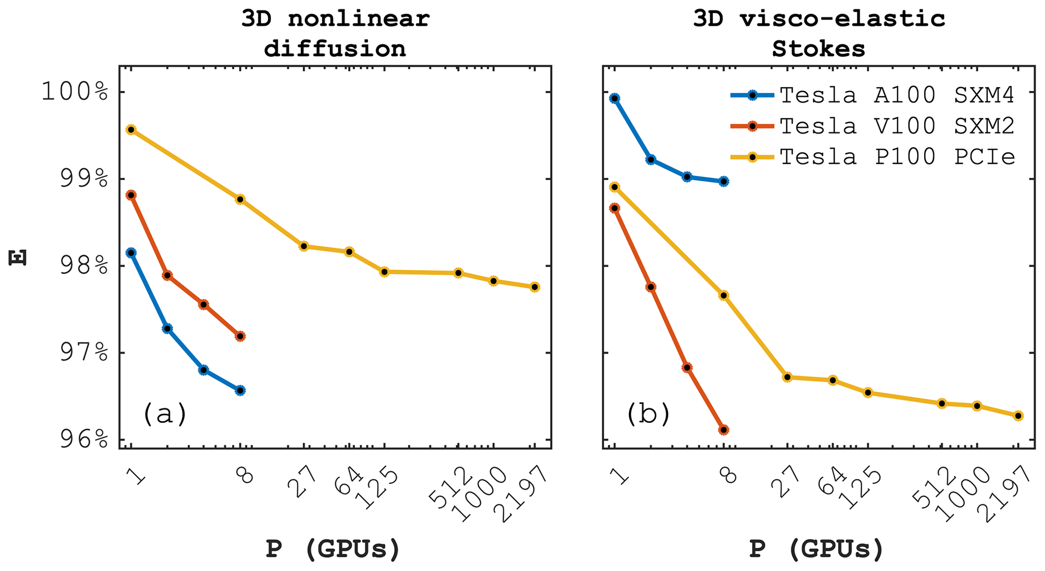
Figure 11Parallel efficiency E as function of 1–8 Tesla A100 SXM4, 1–8 Tesla V100 SXM2, and 1–2197 Tesla P100 Nvidia GPUs (P). Weak-scaling benchmark for (a) the 3D nonlinear diffusion solver and (b) the 3D visco-elastic Stokes flow solver based on a 3D Julia implementation using ParallelStencil.jl and ImplicitGlobalGrid.jl.
7.4 Multiple-inclusions parametric study
We perform a multiple-inclusions benchmark to assess the robustness of the developed accelerated PT method. We vary the viscosity contrast from 1 to 9 orders of magnitude to demonstrate the successful convergence of iterations, even for extreme cases, that might arise in geophysical applications such as strain localisation. Further, we vary the number of inclusions from 1 to 46 to verify the independence of convergence on the “internal geometry” of the problem. For each combination of viscosity ratio and number of inclusions, we perform a series of simulations varying the iteration parameter Re to assess the influence of the problem configuration on its optimal value, and to verify whether the analytical prediction obtained by the dispersion analysis remains valid over the considered parameter range.
For this parametric study, we considered a computational grid consisting of cells. At lower resolutions the convergence deteriorates, resulting in configurations of non-converging large viscosity contrasts. A high-resolution grid is thus necessary for resolving the small-scale details of the flow. We also adjust the nonlinear tolerance for the iterations to 10−5 and 10−3 for momentum and mass balance, respectively, given our interest in relative dependence of iteration counts on the iteration parameter Re.
Figure 12 depicts the results for the shear-driven flow case. For a single inclusion (Fig. 12a), the optimal value of the iteration parameter Re does not differ significantly from the one reported by Eq. (31). Moreover, the theoretical prediction for Re remains valid for all viscosity contrasts considered in the study. For problem configurations involving 14 and 46 inclusions (Fig. 12b and c, respectively), the minimal number of iterations is achieved for values of Re close to the theoretical prediction, only for the viscosity contrast of 1 order of magnitude. For a larger viscosity contrast, the optimal value of Re appears to be lower than theoretically predicted, and the overall iteration count is significantly higher. These iteration counts reach 40nx at the minimum among all values of Re for a given viscosity ratio, and >50nx for non-optimal values of Re.
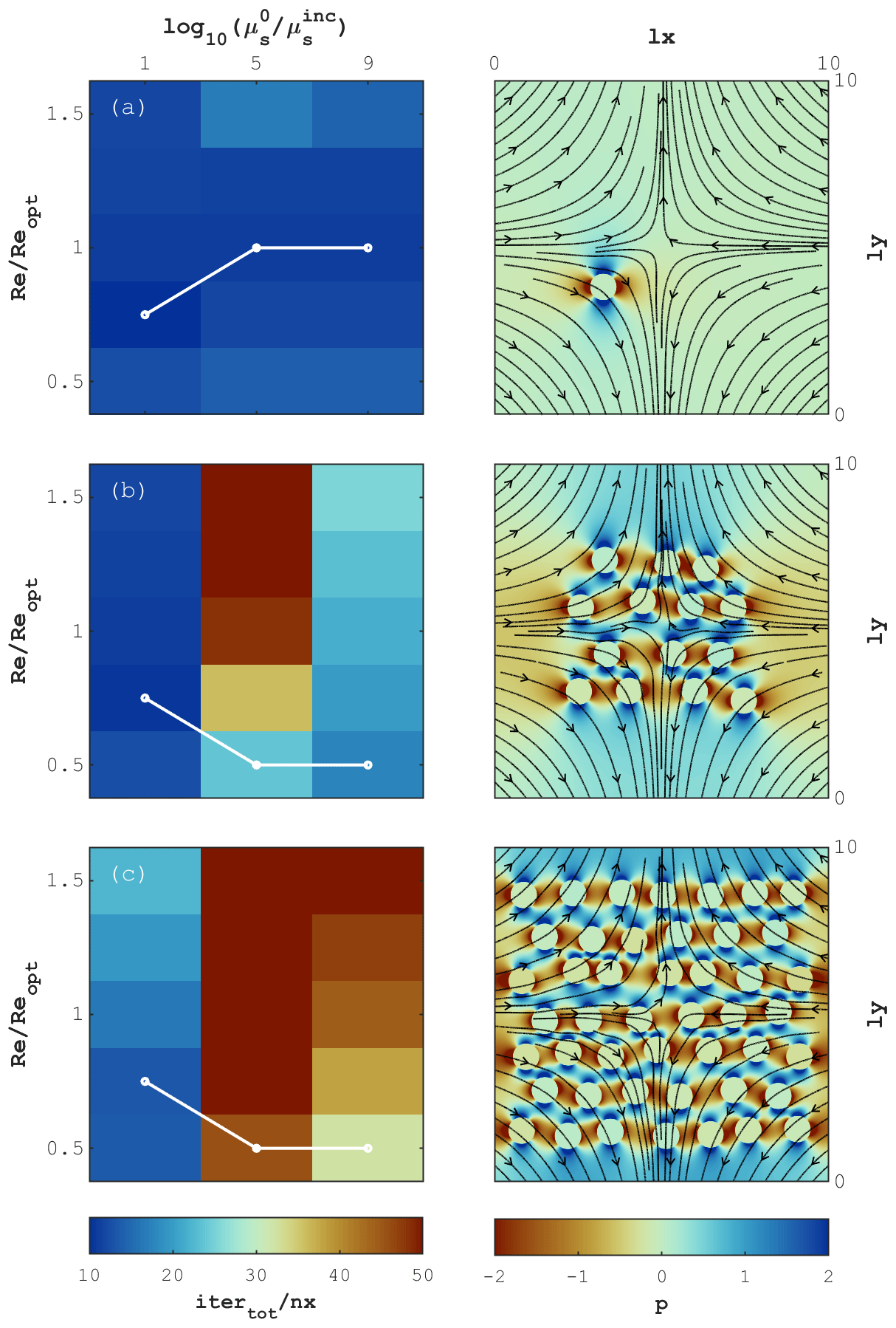
Figure 12Pure shear-driven flow. The left column reports the number of iterations for different values of viscosity ratio and ratio of numerical Reynolds number Re to the theoretically predicted value Reopt. Connected white dots indicate the value of Re at which the minimal number of iterations is achieved. The right column depicts the distribution of pressure and velocity streamlines. Panels (a), (b) and (c) correspond to problem configurations involving 1, 14 and 46 inclusions, respectively.
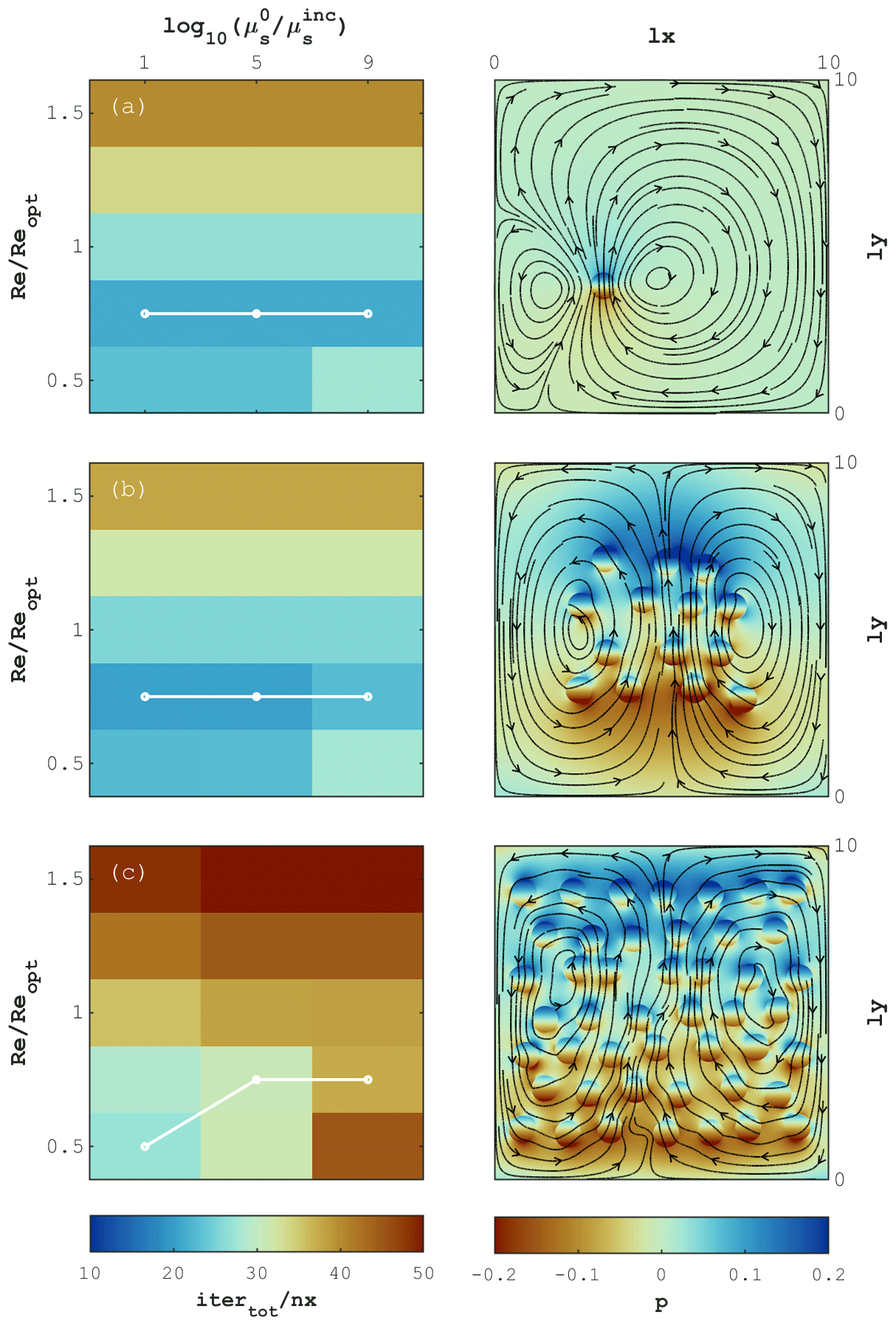
Figure 13Buoyancy-driven flow. The left column reports the number of iterations for different values of viscosity ratio and ratio of numerical Reynolds number Re to the theoretically predicted value Reopt. Connected white dots indicate the value of Re at which the minimal number of iterations is achieved. The right column depicts the deviation of pressure from hydrostatic distribution and velocity streamlines. Panels (a), (b) and (c) correspond to problem configurations involving 1, 14 and 46 inclusions, respectively.
For buoyancy-driven flow (Fig. 13), the convergence of iterations is less sensitive to both the number of inclusions and the viscosity ratio. The observed drift in the optimal value of Re could be partly attributed to the lack of a good preconditioning technique. In this study, we specify the local iteration parameters, and (see Sect. 2.3), in each grid cell based on the values of material parameters, which could be regarded as a form of diagonal (Jacobi) preconditioning. This choice is motivated by the parallel scalability requirements of GPU and parallel computing. Even without employing more advanced preconditioners, our method remains stable and successfully converges for viscosity contrasts up to 9 orders of magnitude, though at the cost of increased number of iterations. The physically motivated iteration strategy enables one to control the stability of iterations through the single CFL-like parameter (see Sect. 2.1.2).
In both shear-driven and gravity-driven problem setups, the convergence is significantly slower than that of the single-centred inclusion case. This slowdown could be explained by the complicated internal geometry involving non-symmetrical inclusion placement featuring huge viscosity contrasts which results in a stiff system.
7.5 Non-similar domain aspect ratio
In geoscientific models that resolve e.g. flow fields for ice sheets and glaciers evolution, lithospheric deformation, or atmospheric and oceanic circulation, there are usually orders of magnitude differences between horizontal and vertical scales. Such domain configurations feature a large aspect ratio that may challenge the solvers because of the presence of more orders-of-magnitude grid cells in the horizontal than the vertical dimensions. Here we systematically investigate the convergence of the 2D visco-elastic Stokes flow while varying the aspect ratio defined as from 1 to 8. We repeat the initial condition of the circular inclusion 1 to 8 times in the x direction to investigate the sensitivity of the accelerated PT solver on the domain aspect ratio. We proportionally increase the number of grid cells in order to keep a constant cell aspect ratio of 1. We report the normalised number of iterations to remain constant for all 5 investigated resolutions when the aspect ratio equals 1 (Fig. 14). The number of normalised iteration counts does not vary significantly while increasing the aspect ratio, independently of the employed resolution. Note that we see a slight dependence of the optimal iteration parameter Re on the aspect ratio.
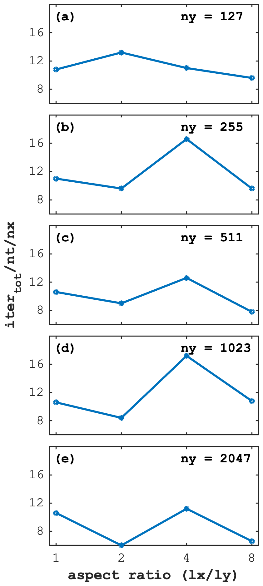
Figure 14Iteration count scaled by the number of time steps (nt) and by the number of grid cells in the x direction (nx) as a function of increasing domain aspect ratios for 5 different numerical resolutions (a)–(e), respectively. The y-direction domain length is kept constant while the x-direction domain length and number of grid cells nx is increased up to 8 times. We use an identical 2D configuration as in the main study with the only difference being the nonlinear tolerance set here to .
To demonstrate the versatility of the approach, we tackle the nonlinear mechanical problem of strain localisation in 2D and 3D. In the following applications we consider an E-VP rheological model, thus the serial viscous damper is deactivated and the flow includes effects of compressibility and plastic dilatancy. We assume a small-strain approximation. Hence, the deviatoric strain rate tensor may be decomposed in an additive manner in Eq. (42). A similar decomposition is assumed for the divergence of velocity in Eq. (43). The plastic model is based on consistent elasto-viscoplasticity and the yield function is defined as
where τII is the second stress invariant, ϕ is the friction angle, μvp is the viscoplastic viscosity and c is the cohesion. At the trial state, Ftrial is evaluated assuming no plastic deformation (). Cohesion strain softening is applied and the rate of c is expressed as
where h is a hardening/softening modulus. Viscoplastic flow is non-associated and the potential function is expressed as
where ψ is the dilatancy angle. If F≥0, viscoplastic flow takes place and the rate of the plastic multiplier is positive and defined as
The initial model configuration assumes a random initial cohesion field. Pure shear kinematics are imposed at the boundaries of the domain (see Sect. 5.2). The reader is referred to Duretz et al. (2019a) for the complete set of material parameters. We only slightly modify the value of μvp with respect to Duretz et al. (2019a), such that Pa s−1 in the present study.
8.1 Performance benefits for desktop-scale computing
Besides the potential to tackle nonlinear multi-physics problems at supercomputer-scale, the ability to solve smaller-scale nonlinear problems remains an important aspect. Here we investigate wall times for the simulation of the previously-described E-VP shear-band formation in 2D (Fig. 15). We compare a MATLAB-based direct-iterative (DI) and a Julia GPU-based PT solver, respectively. The M2Di MATLAB solver routines (Räss et al., 2017) rely on a Newton linearisation of the nonlinear mechanical problem (Duretz et al., 2019a) and use a performant DI solver to compute Newton steps. The solver combines outer Powell–Hestenes and inner Krylov iterations (Global Conjugate Residual) that are preconditioned with the Cholesky factorisation of the symmetrised Jacobian (Räss et al., 2017). In the 2D PT solver, written in Julia using the ParallelStencil.jl packages, the evaluation of nonlinearities is embedded in the pseudo-time integration loop. The timings reported for the DI and PT schemes were produced on a 2.9 GHz Intel Core i5 processor and on a single Nvidia Tesla A100 GPU, respectively (Fig. 15a). Each simulation resolves 100 physical (implicit) time steps and we report the total accumulated plastic strain (Fig. 15b) and the associated pressure fields (Fig. 15c). Models were run on resolutions involving 622 to 5102 and up to 10222 grid cells for the DI and PT scheme, respectively. As expected for 2D computations, reported wall times are lower using the DI scheme at very low resolutions of nx=62. However, it is interesting to observe that the GPU-accelerated PT scheme can deliver comparable wall times at already relatively low resolutions (nx≈126). For numerical resolution of nx=510, the GPU-based PT solver outperforms the DI solver by a factor ≈6 resulting in a wall time of ≈20 minutes to resolve the 100 physical time steps (see dashed lines on Fig. 15a). The employed CPU and GPU can be considered as common devices on current scientific desktop machines. We can thus conclude that the use of the GPU-accelerated PT scheme is a viable and practical approach to solve nonlinear mechanical problems on a desktop-scale computer. Moreover the proposed PT scheme has already turned out to be beneficial over common approaches (DI schemes) at relatively low resolutions.
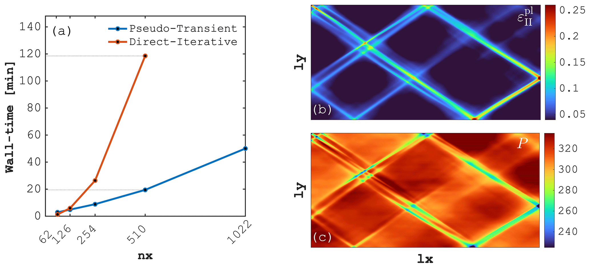
Figure 15Performance comparison between the pseudo-transient (PT) and direct-iterative (DI) method resolving 2D shear-band formation out of a random noise cohesion field. (a) Wall time in minutes as a function of numerical grid resolution in x direction (). The dashed lines connect wall times for nx=510 from both solvers. Panels (b) and (c) depict total accumulated plastic strain and pressure [MPa], respectively, from the 1022×1022 resolution 2D PT-GPU simulation.
8.2 High-resolution 3D results
We present preliminary 3D results of the spontaneous development of visco-plastic shear bands in pure shear deformation from an initial random cohesion field (Fig. 16). These 3D results further demonstrate the versatility of the PT approach, enabling the seamless port of the 2D E-VP algorithm to 3D, extending recent work by Duretz et al. (2019a) to tackle 3D configurations. We generate the 3D initial condition, a Gaussian random field with an exponential co-variance function, following the approach described in Räss et al. (2019b), available through the ParallelRandomFields.jl Julia package (Räss and Omlin, 2021). We perform 100 implicit loading steps using the accelerated PT method and execute the parallel Julia code relying on ParallelStencil.jl and ImplicitGlobalGrid.jl on 8 Tesla V100 on the Volta node. The scalability of the 3D E-VP implementation is comparable to the 2D version (Fig. 15a) with similar discrepancies as reported for the visco-elastic Stokes case (Fig. 7).
Both the 2D and 3D E-VP algorithms require only minor modifications of the visco-elastic Stokes solver discussed throughout this paper to account for brittle failure, deactivation of the serial viscous damper and viscoplastic regularisation without significantly affecting the convergence rate provided by the second-order method. These results support the robustness of the approach, predicting elasto-plastic deformation and capturing brittle failure categorised as a rather “stiff” problem which challenges the numerical solvers accordingly.
The continuous development of many-core devices, with GPUs at the forefront, increasingly shapes the current and future computing landscape. The fact that GPUs and the latest multi-core CPUs turn classical workstations into personal supercomputers is exciting. Tackling previously impossible numerical resolutions or multi-physics solutions becomes feasible as a result of technical progress. However, the current chip design challenges legacy serial and non-local or sparse matrix-based algorithms, seeking solutions to partial differential equations. Naturally, solution strategies designed to specifically target efficient large-scale computations on supercomputers perform most efficiently on GPUs and recent multi-core CPUs, as the algorithms used are typically local and minimise memory accesses. Moreover, efficient strategies will not or only modestly rely on global communication and as a result, exhibit close to optimal scaling.
We introduced the PT method in light of, mostly, iterative type of methods such as dynamic relaxation and semi-iterative algorithms (see, e.g. Saad, 2020, for additional details). These classical methods, as well as the presented accelerated PT method, implement “temporal” damping by considering higher-order derivatives with respect to pseudo-time. This contrasts with multi-grid or multi-level methods, building upon a “spatial” strategy based on space discretisation properties to damp the low-frequency error modes. Multi-grid, or multi-level methods are widely used to achieve numerical solutions in analogous settings as described here (Brandt, 1977; Zheng et al., 2013). Furthermore, multi-grid methods may achieve convergence in O(nx) iterations by employing an optimal relaxation algorithm (Bakhvalov, 1966).
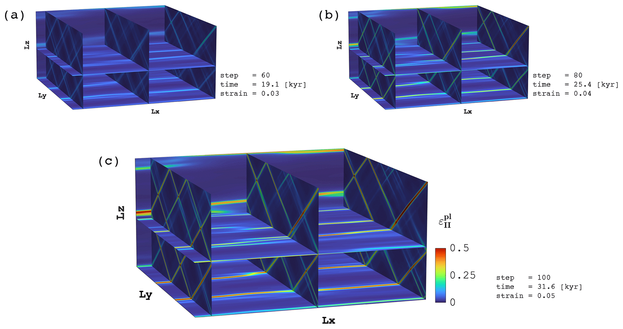
Figure 16Total accumulated plastic strain distribution for a multi-GPU replica of the 2D calculation (Fig. 15b) resolving 3D shear-band formation out of a random noise cohesion field. The numerical resolution includes grid cells. Panels depict elasto-plastic shear-band formation after (a) 60 steps (corresponding 19.1 kyr and a strain of 0.03), (b) 80 steps (corresponding 25.4 kyr and a strain of 0.04) and (c) 100 steps (corresponding 31.6 kyr and a strain of 0.05).
Besides their scalable design, most iterative methods are challenged by configurations including heterogeneities and large contrasts in material parameters, motivated by typical applications to a variety of geodynamics problems (e.g. Baumgardner, 1985; Tackley, 1996; May et al., 2015; Kaus et al., 2016). Well-tuned robust multi-grid solvers may overcome these limitations at the cost of more complex implementations. Our systematic investigation results (Sect. 5.2) suggest, however, that the PT method performs promisingly well, and at no specific additional design efforts w.r.t. the basic accelerated PT method implementation. Beyond single-phase mechanical considerations, the accelerated PT method delivers accurate solutions in tightly coupled and nonlinear multi-physics problems (e.g. Duretz et al., 2019b; Räss et al., 2019a, 2020; Wang et al., 2021).
The ease of implementation is listed among the main advantages of the accelerated PT method over other more complex ones, e.g. multi-grid. Particularly, all nonlinearities can be relaxed within a unique iteration loop, as reported in the nonlinear diffusion results (Sect. 7.1). Often, due to the properties of the problem, the number of iterations does not exceed or is even less than that in the case of constant coefficients. Other methods, in which nonlinear iterations are performed separately from the linear solver, cannot take advantage of the details of the physical process to reduce iteration counts. Also, for significantly nonlinear problems, e.g. associated with plastic strain localisation, thermomechanical shear-heating or two-phase fluid focusing, the physical processes occur on multi-spatial scales. Thus, ensuring an accurate description of these multi-scale solutions requires a high-resolution computational grid. It may be challenging for a coarse level multi-grid solver to provide sufficient information in order to accurately resolve small-scale details that are only resolvable on the fine grid. Note that for analogous reasons, multi-grid methods are often used as a preconditioner for other iterative algorithms rather than the solution method.
Besides seeking optimal convergence of the algorithm, the implementation efficiency also favours the accelerated PT method; the approach is simple but efficient, making it possible to further implement advanced optimisations such as explicit shared memory usage and register handling. The choice of a Cartesian regular grid allows static and regular memory access patterns, resulting in access optimisation possibilities and balanced interprocess communications. Additionally, the absence of global reduction in the algorithm avoids severe bottlenecks. Finally, the amount of data transferred in the accelerated PT method is minimal, which allows achieving near-ideal scaling on distributed-memory systems, as reported in Sect. 7.3.2. Previous studies (e.g. Räss et al., 2018; Duretz et al., 2019b; Räss et al., 2019a, 2020) successfully implemented most of the algorithm designs presented here, although relying on a slightly different PT acceleration implementation (see Appendix B).
The main task in the design of PT methods is the estimation of optimal iteration parameters. For that, the spectral radius of the finite-difference operator is often approximated based on the Gershgorin circle theorem (Papadrakakis, 1981). In this paper, we propose an alternative derivation of the PT algorithm which is based entirely on a physical analogy. The analysis of the convergence rate can be carried out within the framework of the spectral analysis of continuous equations, rather than the finite-dimensional space discretisation. The advantage of this approach relies on the availability of a physical interpretation of the iteration parameters, as well as on a clear separation of physics and numerics. For example, we show that for visco-elastic Stokes flow (Sect. 2.4), the PT iteration parameters depend on the Reynolds number and the bulk-to-shear elastic modulus ratio. The stability of the iterative process is ensured by a choice of pseudo-physical material properties that is consistent with the conditions obtained on the basis of a von Neumann stability analysis.
The determination of the optimal iterative parameters is thereby reduced to the search for the optimal values of the dimensionless physical numbers that describe the properties of the underlying physical process. The addition of new physical processes, such as heat conduction, two-phase flow and chemical reactions will lead to the natural emergence of new dimensionless parameters. Since many physical processes have a similar or even identical mathematical description, it is expected that the derivation of the accelerated PT method for such processes can be carried out similarly to those already developed. In this paper, such a derivation is provided for several important processes, namely, the linear and nonlinear diffusion, diffusion–reaction, non-stationary diffusion, and the visco-elastic Stokes problem. The efficiency of the accelerated PT method is demonstrated for essentially nonlinear problems, as well as for the problems with large contrasts in the material properties.
Recently, Wang et al. (2021) studied fluid flow in deformable porous media using an analogous numerical integration scheme. They show that under certain assumptions, the equations governing the dynamics of such two-phase flows reduce to a “double-damped wave equation” system which is mathematically equivalent to the Eqs. (12) and (6) describing the diffusion–reaction process (Sect. 2.1.3). They also report the optimal parameters obtained by dispersion analysis of these equations. These parameters are formulated by Wang et al. (2021) in terms of dimensional physical parameters. Through appropriate rescaling it is possible to recover the non-dimensional form presented in Sect. 2.1.3. We believe that our derivation in terms of non-dimensional variables helps to reveal the analogy between seemingly different physical properties and facilitates reusing the derived iteration parameters for various applications. We provide analysis for the variety of physical processes, including incompressible Stokes flow, in a unified manner, filling some of the gaps missing in previous studies.
The scalability of the accelerated PT method as a function of numerical resolution permits the prediction of the total iteration count, here for the nonlinear diffusion and the visco-elastic Stokes in 3D. The weak-scaling benchmark results provide the time per iteration as a function of the numerical resolution. Combining this information, it is possible to predict the time-to-solution or wall time (Table 2) needed to resolve nonlinear diffusion and visco-elastic Stokes flow on 66323 and 49553 grid cells, respectively, on 2197 Nvidia Tesla P100 GPUs on the Piz Daint supercomputer at CSCS. Single-GPU problem size scaling results for different GPU architectures further permit the extrapolation of these wall times to the Nvidia Ampere or Volta architecture for example, as time per iteration is directly proportional to the effective memory throughput Teff. There is a 3.0× and 1.5× increase in Teff on the A100 and V100 compared to the P100 architecture, respectively, resulting in wall time in the order of 2.5 min and 2.4 h on a A100 powered system and of 5 min and 4.8 h on a V100 powered system, for the nonlinear diffusion and the visco-elastic Stokes solver, respectively.
Table 2Wall-time prognostic for resolving the nonlinear diffusion and the visco-elastic Stokes 3D Julia multi-GPU applications on 2197 (133) Nvidia Tesla P100 GPUs on the Piz Daint supercomputer at CSCS.
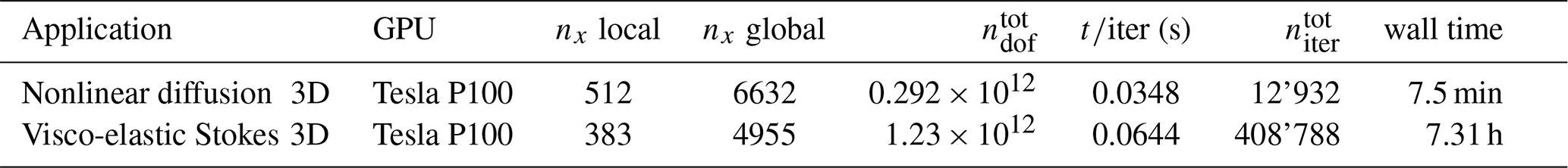
In practical applications, the patterns of the flow may change drastically throughout the simulation owing to the spontaneous flow localisation or evolution of the interface between immiscible phases with significantly different properties. It is a requirement for the numerical method to be robust with respect to such changes. The iterative algorithm is expected to converge even in extreme cases, e.g. in the presence of sharp gradients across material properties, and the iteration parameters should be insensitive to arbitrary changes in the internal geometry. We present a parametric study to assess the robustness of the accelerated PT method for typical building blocks for geophysical applications. We considered shear- and buoyancy-driven flows with multiple randomly distributed inclusions in a viscous matrix as proxies for more realistic problem formulations. We show that our method is capable of modelling flows with viscosity contrasts up to 9 orders of magnitude. The values of optimal iteration parameters obtained by the means of systematic simulation runs do not change significantly for a wide range of material properties and internal configurations of the computational domain. We observe the significant slowdown in convergence for viscosity contrasts larger than 5 orders of magnitude in some of the considered cases. These results are expected, given the ill-conditioned problem and thus motivate development of a scalable preconditioner suitable for massively parallel GPU workloads. The application of a robust preconditioner, with reference to previous discussions, may help to partly alleviate slow convergence. However, for viscosity contrasts of 6 orders of magnitude and more, a significant increase in the number of iterations may be legitimate (May et al., 2015).
The numerical application to resolve shear-banding in elasto-viscoplastic media in 3D supports the versatility and the robustness of the presented approach putting emphasis on successfully handling complex rheology. These examples complement recent studies employing the accelerated PT method to resolve spontaneous localisation owing to multi-physics coupling (Räss et al., 2018, 2019a, 2020; Duretz et al., 2019b) and entire adjoint-based inversion frameworks (Reuber et al., 2020). The Sect. B of the Appendix provides connections of the presented analysis with previous work.
The current HPC landscape redefines the rules governing applications' performance where the multi-core processors' massive parallelism imposes a memory-bound situation. Our work shows that simple dynamic relaxation schemes can be employed efficiently to solve parabolic and nonlinear systems, upon transforming the equations into hyperbolic expressions. The transformation includes the addition of physics-inspired terms which enable the possibility to retrieve optimal parameters that minimise the iteration counts. The optimisation procedure includes von Neumann stability and dispersion analysis for the pseudo-physical parameters. Moreover, the conciseness of the accelerated PT approach permits the applications to execute at effective memory throughput rate the approaching memory copy rates (a theoretical upper bound) of latest GPUs. Further, hiding communication behind computations permits the achievement of parallel efficiency of more than 96 % on various distributed-memory systems and up to 2197 GPUs. The physics we selected for the numerical experiments represent key building blocks to further tackle various multi-physics coupling, usually the combination of mechanical and diffusive processes. Our systematic results on the multi-inclusion setup with huge viscosity contrasts provide some preliminary results assessing the robustness of the accelerated PT method, which we further employ to resolve shear-band formation in 3D as a result of plastic yielding in E-VP materials. Our study paves the way for resolving coupled and nonlinear multi-physics applications in natural sciences and engineering on extremely high resolutions on the next generation of exascale-capable supercomputers, revamping elegant iterative techniques and implementing them with the portable Julia language.
A1 First-order pseudo-transient (PT) diffusion
Let the total pseudo-time required to reach convergence be τtot. To estimate τtot and the number of iterations in the numerical implementation of the method, we consider the deviation ϵ of H from the exact solution to Eq. (4). Linearity of the problem makes it possible to reformulate Eq. (5) in terms of ϵ:
where . Equation (A1) is subject to homogeneous boundary conditions: .
We study the convergence rate of the PT method by performing the dispersion analysis of Eq. (A1). The general solution to the Eq. (A1) with homogeneous Dirichlet boundary conditions has the following form:
where is the characteristic velocity scale of diffusion, k is the wavenumber, Ek and λk are the initial amplitude and the decay rate of the wave with wavenumber k, respectively. Only values of k≥1 are accounted for in Eq. (A2), because for other values of k, homogeneous boundary conditions are not satisfied.
We are interested in the exponential decay rate values λk, because they indicate the total time it takes for the error component with wavelength πk to vanish. It is sufficient to consider only one typical term from the solution Eq. (A2):
Substituting Eq. (A3) into Eq. (A1) gives
The dispersion relation Eq. (A4) indicates that the harmonics with higher wavenumbers decay faster than the ones with smaller wavenumbers. Therefore, the total time τtot to convergence is controlled by the component of ϵ with the smallest wavenumber k=1. If the required non-dimensional accuracy, i.e. upper bound on ϵ, is ϵtol, then τtot can be obtained by solving Eq. (A3) for τ at k=1 and :
The stability analysis of Eq. (5) in discretised form suggests that the maximal time step Δτ allowed by the explicit integration scheme is proportional to the grid spacing Δx squared: . If the computational grid is uniform, as it is the case in this paper, L=nxΔx, where nx is the number of grid cells. Assuming τtot=nitΔτ, where nit is the number of PT iterations required for convergence, and substituting expressions for L and τtot into the Eq. (A5), we obtain
Thus, the number of pseudo-time iterations required for convergence must be proportional to .
A2 Accelerated PT diffusion
Similar to the previous case, we reformulate the problem in terms of deviation from the exact solution and consider the typical term from the Fourier series expansion:
Substituting Eq. (A7) into Eq. (7) gives the following dispersion relation:
where . The non-dimensional parameter Re can be interpreted as a numerical Reynolds number, or as the inverse of a numerical Deborah number's square root, characterising the ratio between relaxation time θr and characteristic time of diffusion .
Solving the Eq. (A8) for λk yields
Depending on values of Re and k, λk can be complex. The imaginary part of λk, ℑ(λk), contributes to the oscillatory behaviour of the solution, while the real part ℜ(λk) controls the exponential decay of deviation ϵ. The minimum of ℜ(λk) between the two roots of Eq. (A9) indicates the decay rate of the entire solution. This minimum reaches maximal value when both roots of Eq. (A9) are equal, i.e. when the discriminant of Eq. (A9) . Therefore, , but negative Re leads to exponential growth of the term in the solution Eq. (A7), which is non-physical. Finally, since choosing iteration parameters for each wavelength independently is not realistic, we chose Re such that the longest wave with wavenumber k=0 is damped most effectively. The optimal value of Re is then given by
Total pseudo-time τtot required for convergence with tolerance ϵtot is determined in the same way as in the previous case:
The stability analysis of the damped wave equation in discretised form suggests that in a certain range of values of θr, the maximal time step (Alkhimenkov et al., 2021a). The number of pseudo-time iterations required for convergence nit can then be estimated as
and proportional to nx in the accelerated scheme.
A3 Diffusion–reaction
Reformulating Eq. (13) in terms of the difference ϵ between the exact steady-state solution and the PT solution and substituting it into Eq. (A7), one obtains the following dispersion relation:
Introducing the auxiliary parameter , it can be seen that the dispersion relation in Eq. (A13) is now similar to the one reported in Eq. (A8). The solution for λk is now given by
The resulting optimal value is , and the optimal value for Re is obtained by solving for Re:
As expected, in the limit of Da→0, i.e. when the process becomes diffusion-dominated, the optimal value of the parameter Re, determined by Eq. (A15), coincides with the value given by Eq. (A10) in the case of a purely diffusive process.
The number of iterations required to converge to a tolerance ϵtol is
Interestingly, the iteration count estimate given by Eq. (A16) decreases proportionally to . Therefore, the number of iterations for a diffusion–reaction process will always be lower than for a pure diffusion process if Da>0.
A4 Incompressible viscous Stokes
The system of Eqs. (25)–(27) can be reduced to a single equation for velocity vx:
Following the established procedure, we reformulate Eq. (A17) in terms of deviation ϵ from the exact solution, and consider typical terms in the Fourier series expansion of ϵ:
Substituting Eq. (A18) into Eq. (A17), we obtain the following dispersion relation:
Depending on the values of the coefficients, the dispersion relation in Eq. (A19) would have either one real root and two complex conjugate roots or three real roots.
For analysis, it is useful to recast the dispersion relation in Eq. (A19) to depressed form applying a change of variables :
The discriminant of the depressed cubic equation is is . Setting the discriminant of Eq. (A20) to zero yields
Equation (A21) is biquadratic w.r.t. Re. We denote the discriminant of Eq. (A21) by D. For Re to be real, D must be non-negative:
By definition, r is the ratio between the bulk and shear modulus, therefore, r must be positive. Thus, .
By solving Eq. (A21), we obtain the relation between Re and r:
Only the positive branch of the solution is taken in Eq. (A23) because Re must be positive.
When the depressed cubic equation has multiple roots, the simple root is , and the double root is . Substituting expressions for q and p from the dispersion relation in Eq. (A20), and changing variables back to λk from αk, one obtains:

Figure A1Roots of the dispersion relation λk for two branches of the numerical parameter Re. Solid and dashed lines show maximal and minimal roots, respectively.
Substituting Eq. (A23) into Eq. (A24), one obtains roots of the dispersion relation in Eq. (A19) as a function of parameter r. The roots depend monotonously on r for all choices of Re (Fig. A1). The minimal root reaches its maximum value at . The corresponding value of Re is then for k=1.
It is useful to provide an analogy between the presented analysis and some previous studies, namely, PT continuation model by Räss et al. (2018, 2019a, 2020); Duretz et al. (2019b), and early work by Frankel (1950). For this comparison, we consider only a stationary diffusion process with D=const.
We reformulate the damped wave equation, Eq. (7), as a first-order system introducing R, the pseudo-time derivative of H:
In all mentioned studies the numerical discretisation of Eqs. (B1) and (B2) were considered. Let fk be the finite-difference operator approximating the right-hand side of Eq. (B2) at time step k. Using a forward Euler scheme for the time integration, one obtains
Let . Rearranging Eqs. (B3) and (B4) to formulate the update-rules for and :
and using the definitions of θr and Δτ reported by Eqs. (10) and (8):
it is evident that, if combined, Eqs. (B5), (B6) and (B7) are equivalent to the formulation of PT continuation method presented in Räss et al. (2018). Substituting Eq. (B6) into Eq. (B5) and expressing in terms of and yields
which is equivalent to the second-order Richardson method proposed in Frankel (1950).
The various software developed and used in the scope of this study is licensed under MIT License. The latest versions of the code is available from GitHub at: https://github.com/PTsolvers/PseudoTransientDiffusion.jl (last access: 16 May 2022) and https://github.com/PTsolvers/PseudoTransientStokes.jl (last access: 16 May 2022). Past and future versions of the software are available from a permanent DOI repository (Zenodo) at: https://doi.org/10.5281/zenodo.6553699 (Räss and Utkin, 2022a) and https://doi.org/10.5281/zenodo.6553714 (Räss and Utkin, 2022b). Both the PseudoTransientDiffusion.jl and the PseudoTransientStokes.jl repositories contain most Julia multi-xPU code examples implementing the accelerated PT method and can be readily used to reproduce the figures of the paper. The codes are written using the Julia programming language. Scaling figures can readily be reproduced using the available data, while all other figures require first executing the Julia scripts to produce the expected data. Refer to the repositories' README for additional information.
LR designed the original study, developed codes and algorithms, realised the Julia at scale implementation, performed scaling and performance benchmarks, created figures and edited the manuscript. IU developed codes and algorithms, performed the dispersion analysis and the parametric study, created figures and edited the manuscript. TD contributed to the original study design, realised the desktop-scale computation benchmark, performed the E-VP model investigations, created figures and edited the manuscript. SO developed the building blocks for implementing Julia at scale and the effective memory throughput metric, deployed Julia on Piz Daint, provided scalable architecture-agnostic PDE solver implementation and edited the manuscript. YYP provided early work on accelerated PT methods, helped out with the dispersion analysis, contributed to methodological advances to allow PDE solver implementations on GPUs.
The contact author has declared that none of the authors has any competing interests.
Publisher's note: Copernicus Publications remains neutral with regard to jurisdictional claims in published maps and institutional affiliations.
We thank Boris Kaus, Stefan Schmalholz and Mauro Werder for stimulating discussions. We thank Lawrence H. Wang, Boris Kaus and an anonymous reviewer for their suggestions to improve the manuscript. We acknowledge the Swiss Geocomputing Centre, University of Lausanne, for computing resources on the Octopus supercomputer and are grateful to Philippe Logean for continuous technical support.
This research has been supported by the Swiss University Conference and the Swiss Council of Federal Institutes of Technology through the Platform for Advanced Scientific Computing (PASC) program and the Swiss National Supercomputing Centre (CSCS) (project ID c23). Ivan Utkin and Yuri Y. Podladchikov received financial support from the Russian Ministry of Science and Higher Education (project no. 075-15-2019-1890). Publisher's note: the article processing charges for this publication were not paid by a Russian or Belarusian institution.
This paper was edited by James Kelly and reviewed by Lawrence Hongliang Wang, Boris Kaus, and one anonymous referee.
Alamatian, J.: A new formulation for fictitious mass of the Dynamic Relaxation method with kinetic damping, Comput. Struct., 90–91, 42–54, https://doi.org/10.1016/j.compstruc.2011.10.010, 2012. a
Alkhimenkov, Y., Khakimova, L., and Podladchikov, Y.: Stability of discrete schemes of Biot's poroelastic equations, Geophys. J. Int., 225, 354–377, https://doi.org/10.1093/gji/ggaa584, 2021a. a, b
Alkhimenkov, Y., Räss, L., Khakimova, L., Quintal, B., and Podladchikov, Y.: Resolving Wave Propagation in Anisotropic Poroelastic Media Using Graphical Processing Units (GPUs), J. Geophys. Res.-Sol. Ea., 126, 7, https://doi.org/10.1029/2020JB021175, 2021b. a
Bakhvalov, N. S.: On the convergence of a relaxation method with natural constraints on the elliptic operator, USSR Comp. Math. Math.+, 6, 101–135, https://doi.org/10.1016/0041-5553(66)90118-2, 1966. a
Barnes, M. R.: Form Finding and Analysis of Tension Structures by Dynamic Relaxation, International Journal of Space Structures, 14, 89–104, https://doi.org/10.1260/0266351991494722, 1999. a
Baumgardner, J. R.: Three-dimensional treatment of convective flow in the earth's mantle, J. Stat. Phys., 39, 501–511, https://doi.org/10.1007/BF01008348, 1985. a
Besard, T., Foket, C., and De Sutter, B.: Effective Extensible Programming: Unleashing Julia on GPUs, IEEE T. Parall. Distr., 30, 827–841, https://doi.org/10.1109/TPDS.2018.2872064, 2018. a
Besard, T., Churavy, V., Edelman, A., and De Sutter, B.: Rapid software prototyping for heterogeneous and distributed platforms, Adv. Eng. Softw., 132, 29–46, 2019. a
Bezanson, J., Edelman, A., Karpinski, S., and Shah, V. B.: Julia: A fresh approach to numerical computing, SIAM Rev., 59, 65–98, https://doi.org/10.1137/141000671, 2017. a, b
Brandt, A.: Multi-level adaptive solutions to boundary-value problems, Math. Comput., 31, 333–390, https://doi.org/10.1090/S0025-5718-1977-0431719-X, 1977. a, b
Byrne, S., Wilcox, L. C., and Churavy, V.: MPI.jl: Julia bindings for the Message Passing Interface, Proceedings of the JuliaCon Conferences, 1, 68, https://doi.org/10.21105/jcon.00068, 2021. a
Cassell, A. C. and Hobbs, R. E.: Numerical stability of dynamic relaxation analysis of non-linear structures, Int. J. Numer. Meth. Eng., 10, 1407–1410, https://doi.org/10.1002/nme.1620100620, 1976. a
Chester, M.: Second sound in solids, Phys. Rev., 131, 2013–2015, https://doi.org/10.1103/PhysRev.131.2013, 1963. a
Costa, A.: Permeability-porosity relationship: A reexamination of the Kozeny-Carman equation based on a fractal pore-space geometry assumption, Geophys. Res. Lett., 33, L02318, https://doi.org/10.1029/2005GL025134, 2006. a
Cox, S. and Zuazua, E.: The rate at which energy decays in a damped string, Commun. Part. Diff. Eq., 19, 213–243, https://doi.org/10.1080/03605309408821015, 1994. a
Cundall, A. P.: Explicit finite differnce method in geomechanics, Second Int. Conf. Numerical Methods in Geomechanics, Blacksburg, 1976, 1, 132–150, 1976. a
Duretz, T., de Borst, R., and Le Pourhiet, L.: Finite Thickness of Shear Bands in Frictional Viscoplasticity and Implications for Lithosphere Dynamics, Geochem. Geophy. Geosy., 20, 5598–5616, https://doi.org/10.1029/2019GC008531, 2019a. a, b, c, d, e, f
Duretz, T., Räss, L., Podladchikov, Y., and Schmalholz, S.: Resolving thermomechanical coupling in two and three dimensions: spontaneous strain localization owing to shear heating, Geophys. J. Int., 216, 365–379, https://doi.org/10.1093/gji/ggy434, 2019b. a, b, c, d, e, f
Eager, D. L., Zahorjan, J., and Lazowska, E. D.: Speedup versus efficiency in parallel systems, IEEE T. Comput., 38, 408–423, https://doi.org/10.1109/12.21127, 1989. a
Frankel, S. P.: Convergence rates of iterative treatments of partial differential equations, Mathematical Tables and Other Aids to Computation, 4, 65–75, 1950. a, b, c, d, e
Fuhrer, O., Chadha, T., Hoefler, T., Kwasniewski, G., Lapillonne, X., Leutwyler, D., Lüthi, D., Osuna, C., Schär, C., Schulthess, T. C., and Vogt, H.: Near-global climate simulation at 1 km resolution: establishing a performance baseline on 4888 GPUs with COSMO 5.0, Geosci. Model Dev., 11, 1665–1681, https://doi.org/10.5194/gmd-11-1665-2018, 2018. a
Gaitonde, A. L.: A dual-time method for two-dimensional unsteady incompressible flow calculations, Int. J. Numer. Meth. Eng., 41, 1153–1166, https://doi.org/10.1002/(SICI)1097-0207(19980330)41:6<1153::AID-NME334>3.0.CO;2-9, 1998. a
Gustafson, J. L.: Reevaluating Amdahl's law, Commun. ACM, 31, 532–533, https://doi.org/10.1145/42411.42415, 1988. a
Hackbusch, W.: Multi-Grid Methods and Applications, vol. 4, Springer Series in Computational Mathematics, Springer, Berlin, Heidelberg, https://doi.org/10.1007/978-3-662-02427-0, 1985. a
Hoemmen, M. F.: Communication-avoiding Krylov subspace methods, PhD thesis, EECS Department, University of California, Berkeley, http://www2.eecs.berkeley.edu/Pubs/TechRpts/2010/EECS-2010-37.html (last access: 16 May 2022), 2010. a
Jordan, P. M. and Puri, A.: Digital signal propagation in dispersive media, J. Appl. Phys., 85, 1273–1282, https://doi.org/10.1063/1.369258, 1999. a
Kaus, B. J. P., Popov, A. A., Baumann, T. S., Püsök, A. E., Bauville, A., Fernandez, N., and Collignon, M.: Forward and Inverse Modelling of Lithospheric Deformation on Geological Timescales, in: NIC Symposium 2016, Jülich, Germany, 11–12 February 2016, edited by: Binder, K., Müller, M., Kremer, A., and Schnurpfeil, A., 48, 299–307, Forschungszentrum Jülich, Jülich, 2016. a
Kilic, B. and Madenci, E.: Structural stability and failure analysis using peridynamic theory, Int. J. NonLin. Mech., 44, 845–854, https://doi.org/10.1016/j.ijnonlinmec.2009.05.007, 2009. a
Kumar, V., Grama, A., Gupta, A., and Karypis, G.: Introduction to parallel computing, Benjamin/Cummings Redwood City, CA, 110, ISBN 0805331700, 1994. a
Mandal, J., Sonawane, C., Iyer, A., and GosaviInamdar, S.: Incompressible flow computations over moving boundary using a novel upwind method, Comput. Fluid., 46, 348–352, 2011. a
Maxwell, J. C.: IV. On the dynamical theory of gases, Philos. T. R. Soc. Lond., 157, 49–88, https://doi.org/10.1098/rstl.1867.0004, 1867. a
May, D., Brown, J., and Le Pourhiet, L.: A scalable, matrix-free multigrid preconditioner for finite element discretizations of heterogeneous Stokes flow, Comput. Method Appl. M., 290, 496–523, https://doi.org/10.1016/j.cma.2015.03.014, 2015. a, b
McCalpin, J. D.: Memory bandwidth and machine balance in current high performance computers, IEEE computer society technical committee on computer architecture (TCCA) newsletter, 2, 19–25, 1995. a
McKee, S., Tomé, M., Ferreira, V., Cuminato, J., Castelo, A., Sousa, F., and Mangiavacchi, N.: The MAC method, Comput. Fluid., 37, 907–930, https://doi.org/10.1016/j.compfluid.2007.10.006, 2008. a
Omlin, S.: Development of massively parallel near peak performance solvers for three-dimensional geodynamic modelling, PhD thesis, University of Lausanne, https://doi.org/10.48550/ARXIV.2207.08716, 2017. a
Omlin, S. and Räss, L.: ImplicitGlobalGrid.jl, https://github.com/eth-cscs/ImplicitGlobalGrid.jl (last access: 16 May 2022), 2021a. a
Omlin, S. and Räss, L.: ParallelStencil.jl, https://github.com/omlins/ParallelStencil.jl (last access: 16 May 2022), 2021b. a, b
Omlin, S., Räss, L., and Podladchikov, Y.: HPC.m – the MATLAB HPC Compiler and its Use for Solving 3D Poromechanics on Supercomputers, in: Platform for Advanced Scientific Computing Conference (PASC15), 1–3 June 2015, Zurich, Switzerland, ETH Zurich, Zurich, Switzerland, 2015a. a
Omlin, S., Räss, L., and Podladchikov, Y.: From MATLAB to Supercomputing: the MATLAB HPC-Compiler, in: 2nd Frontiers in Computational Physics: Energy Sciences Conference 2015, 3–5 June 2015, Zurich, Switzerland, ETH Zurich, Zurich, Switzerland, 2015b. a
Otter, J.: Computations for prestressed concrete reactor pressure vessels using dynamic relaxation, Nuclear Structural Engineering, 1, 61–75, https://doi.org/10.1016/0369-5816(65)90097-9, 1965. a
Otter, J. R. H., Cassell, A. C., and Hobbs, R. E.: Dynamic relaxation, 35, 633–656, https://doi.org/10.1680/IICEP.1966.8604, 1966. a
Papadrakakis, M.: A method for the automatic evaluation of the dynamic relaxation parameters, Comput. Method Appl. M., 25, 35–48, https://doi.org/10.1016/0045-7825(81)90066-9, 1981. a, b
Pascal, H.: Pressure wave propagation in a fluid flowing through a porous medium and problems related to interpretation of Stoneley's wave attenuation in acoustical well logging, Int. J. Eng. Sci., 24, 1553–1570, https://doi.org/10.1016/0020-7225(86)90163-1, 1986. a
Patankar, S.: Numerical heat transfer and fluid flow, CRC press, https://doi.org/10.1201/9781482234213, 1980. a
Podladtchikov, I. and Podladchikov, Y. Y.: Memory Bound Wave Propagation at Hardware Limit, http://on-demand.gputechconf.com/gtc/2013/video/S3176-Memory-Bound-Wave-Propagation-Hardware-Limit.flv (last access: 16 May 2022), 2013. a
Poliakov, A. N., Cundall, P. A., Podladchikov, Y. Y., and Lyakhovsky, V. A.: An explicit inertial method for the simulation of viscoelastic flow: an evaluation of elastic effects on diapiric flow in two- and three- layers models, Flow and creep in the solar system: observations, modeling and theory, NATO ASI Series, vol. 391, Springer, Dordrecht, 175–195, https://doi.org/10.1007/978-94-015-8206-3_12, 1993. a
Poliakov, A. N. B., Herrmann, H. J., Podladchikov, Y. Y., and Roux, S.: Fractal plastic shear bands, Fractals, 2, 567–581, https://doi.org/10.1142/s0218348x9400079x, 1994. a
Ramesh, G. and Krishnamoorthy, C. S.: Post‐buckling analysis of structures by dynamic relaxation, Int. J. Numer. Meth. Eng., 36, 1339–1364, https://doi.org/10.1002/nme.1620360806, 1993. a
Räss, L. and Omlin, S.: ParallelRandomFields.jl, https://github.com/luraess/ParallelRandomFields.jl (last access: 16 May 2022), 2021. a
Räss, L. and Utkin, I.: PTsolvers/PseudoTransientDiffusion.jl: PseudoTransientDiffusion.jl 1.0.0, Zenodo [code], https://doi.org/10.5281/zenodo.6553699, 2022a. a, b
Räss, L. and Utkin, I.: PTsolvers/PseudoTransientStokes.jl: PseudoTransientStokes.jl 1.0.0, Zenodo [code], https://doi.org/10.5281/zenodo.6553714, 2022b. a, b
Räss, L., Duretz, T., Podladchikov, Y. Y., and Schmalholz, S. M.: M2Di: Concise and efficient MATLAB 2-D Stokes solvers using the Finite Difference Method, Geochem. Geophy. Geosy., 18, 755–768, https://doi.org/10.1002/2016GC006727, 2017. a, b
Räss, L., Simon, N. S., and Podladchikov, Y. Y.: Spontaneous formation of fluid escape pipes from subsurface reservoirs, Sci. Rep.-UK, 8, 1–11, 2018. a, b, c, d, e
Räss, L., Duretz, T., and Podladchikov, Y. Y.: Resolving hydro-mechanical coupling in two and three dimensions: Spontaneous channelling of porous fluids owing to decompaction weakening, Geophys. J. Int., 218, 1591–1616, https://doi.org/10.1093/gji/ggz239, 2019a. a, b, c, d, e, f, g
Räss, L., Kolyukhin, D., and Minakov, A.: Efficient parallel random field generator for large 3-D geophysical problems, Comput. Geosci., 131, 158–169, https://doi.org/10.1016/j.cageo.2019.06.007, 2019b. a
Räss, L., Omlin, S., and Podladchikov, Y. Y.: Resolving Spontaneous Nonlinear Multi-Physics Flow Localization in 3-D: Tackling Hardware Limit, https://developer.nvidia.com/gtc/2019/video/S9368 (last access: 16 May 2022), 2019c. a
Räss, L., Licul, A., Herman, F., Podladchikov, Y. Y., and Suckale, J.: Modelling thermomechanical ice deformation using an implicit pseudo-transient method (FastICE v1.0) based on graphical processing units (GPUs), Geosci. Model Dev., 13, 955–976, https://doi.org/10.5194/gmd-13-955-2020, 2020. a, b, c, d, e, f
Reuber, G. S., Holbach, L., and Räss, L.: Adjoint-based inversion for porosity in shallow reservoirs using pseudo-transient solvers for non-linear hydro-mechanical processes, J. Comput. Phys., 423, 109797, https://doi.org/10.1016/j.jcp.2020.109797, 2020. a
Rezaiee-Pajand, M., Kadkhodayan, M., Alamatian, J., and Zhang, L. C.: A new method of fictitious viscous damping determination for the dynamic relaxation method, Comput. Struct., 89, 783–794, https://doi.org/10.1016/J.COMPSTRUC.2011.02.002, 2011. a, b
Richardson, L. F.: IX. The approximate arithmetical solution by finite differences of physical problems involving differential equations, with an application to the stresses in a masonry dam, Philos. T. R. Soc. A, 210, 307–357, https://doi.org/10.1098/rsta.1911.0009, 1911. a
Riley, J. D.: Iteration Procedures for the Dirichlet Difference Problem, Mathematical Tables and Other Aids to Computation, 8, 125–131, https://doi.org/10.2307/2001924, 1954. a, b
Saad, Y.: Iterative methods for linear systems of equations: A brief historical journey, in: Contemporary Mathematics, edited by: Brenner, S., Shparlinski, I., Shu, C.-W., and Szyld, D., American Mathematical Society, Providence, Rhode Island, 754, 197–215, https://doi.org/10.1090/conm/754/15141, 2020. a, b
Shin, D. and Strikwerda, J. C.: Inf-sup conditions for finite-difference approximations of the Stokes equations, J. Aust. Math. Soc. B, 39, 121–134, 1997. a
Swirydowicz, K., Langou, J., Ananthan, S., Yang, U., and Thomas, S.: Low synchronization Gram-Schmidt and generalized minimal residual algorithms, Numer. Linear Algebr., 28, e2343, https://doi.org/10.1002/nla.2343, 2020. a
Tackley, P. J.: Effects of strongly variable viscosity on three-dimensional compressible convection in planetary mantles, J. Geophys. Res.-Sol. Ea., 101, 3311–3332, https://doi.org/10.1029/95JB03211, 1996. a
Trottenberg, U., Oosterlee, C. W. C. W., and Schüller, A.: Multigrid, Academic Press, hardcover ISBN 9780127010700, eBook ISBN 9780080479569, 2001. a
Virieux, J.: P-SV wave propagation in heterogeneous media: Velocity‐stress finite‐difference method, Geophysics, 51, 889–901, https://doi.org/10.1190/1.1442147, 1986. a
Wang, L. H., Yarushina, V., Alkhimenkov, Y., and Podladchikov, Y.: Physics-inspired pseudo-transient method and its application in modelling focused fluid flow with geological complexity, Geophys. J. Int., 229, 1–20, https://doi.org/10.1093/GJI/GGAB426, 2021. a, b, c
Wulf, W. A. and McKee, S. A.: Hitting the memory wall: implications of the obvious, ACM Comp. Ar., 23, 20–24, https://doi.org/10.1145/216585.216588, 1995. a
Young, D. M.: Second-degree iterative methods for the solution of large linear systems, J. Approx. Theory, 5, 137–148, https://doi.org/10.1016/0021-9045(72)90036-6, 1972. a
Zheng, L., Gerya, T., Knepley, M., Yuen, D. A., Zhang, H., and Shi, Y.: GPU implementation of multigrid solver for stokes equation with strongly variable viscosity, in: Lecture Notes in Earth System Sciences, 0, 321–333, Springer, Berlin, Heidelberg, https://doi.org/10.1007/978-3-642-16405-7_21, 2013. a
- Abstract
- Introduction
- The pseudo-transient (PT) method
- Performance and scaling
- The numerical experiments
- The model configurations
- Discretisation
- Results
- Applications to nonlinear mechanical problems with elasto-viscoplastic rheology
- Discussion
- Conclusions
- Appendix A: Dispersion analysis
- Appendix B: Connection to the previous work
- Code availability
- Author contributions
- Competing interests
- Disclaimer
- Acknowledgements
- Financial support
- Review statement
- References