the Creative Commons Attribution 4.0 License.
the Creative Commons Attribution 4.0 License.
 | 25 Jul 2022
swNEMO_v4.0: an ocean model based on NEMO4 for the new-generation Sunway supercomputer
Yuejin Ye
Zhenya Song
Shengchang Zhou
Yao Liu
Bingzhuo Wang
Weiguo Liu
Fangli Qiao
Lanning Wang
The current large-scale parallel barrier of ocean general circulation models (OGCMs) makes it difficult to meet the computing demand of high resolution. Fully considering both the computational characteristics of OGCMs and the heterogeneous many-core architecture of the new Sunway supercomputer, swNEMO_v4.0, based on NEMO4 (Nucleus for European Modelling of the Ocean version 4), is developed with ultrahigh scalability. Three innovations and breakthroughs are shown in our work: (1) a highly adaptive, efficient four-level parallelization framework for OGCMs is proposed to release a new level of parallelism along the compute-dependency column dimension. (2) A many-core optimization method using blocking by remote memory access (RMA) and a dynamic cache scheduling strategy is applied, effectively utilizing the temporal and spatial locality of data. The test shows that the actual direct memory access (DMA) bandwidth is greater than 90 % of the ideal bandwidth after optimization, and the maximum is up to 95 %. (3) A mixed-precision optimization method with half, single and double precision is explored, which can effectively improve the computation performance while maintaining the simulated accuracy of OGCMs. The results demonstrate that swNEMO_v4.0 has ultrahigh scalability, achieving up to 99.29 % parallel efficiency with a resolution of 500 m using 27 988 480 cores, reaching the peak performance with 1.97 PFLOPS.
- Article
(4445 KB) - Full-text XML
- BibTeX
- EndNote


Ocean general circulation models (OGCMs) are numerical models focusing on the properties of oceans based on the Navier–Stokes equations on the rotating sphere with thermodynamic terms for various energy sources (Chassignet et al., 2019). OGCMs are the most powerful tools for predicting the ocean and climate states. As shown in Fig. 1, recent studies indicate that the horizontal resolution of OGCMs used for ocean research has been improved from 5∘ (approximately 500 km) (Bryan et al., 1967; Bryan, 1969) to ∘ (approximately 2 km) (Rocha et al., 2016; Viglione et al., 2018; Dong et al., 2020; Qiu et al., 2018, 2020). However, the small-scale processes in the ocean (Chassignet et al., 2019; Lellouche et al., 2018), which are critical for further reducing the ocean simulation and prediction biases, still cannot be resolved within a 2 km resolution. Therefore, improving the spatial resolution is one of the most important directions of OGCM development.
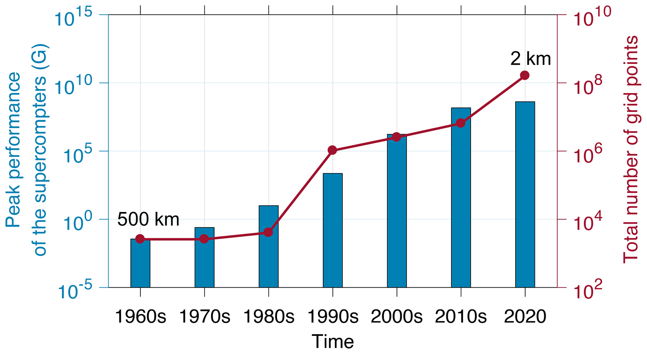
Figure 1Peak performance of the supercomputers (blue bar) and the total number of OGCM grid points (red line) over the past 60 years.
The increase in OGCMs' resolution results in an exponential increase in the demand for computing capabilities. With the doubled horizontal resolution, the amount of calculation increases about 10 times accordingly. However, the enhanced performance of supercomputers makes it feasible to simulate oceans at higher resolutions. Compared to homogeneous systems, which cannot afford the high-power cost of the transition from petaFLOPS supercomputers to exaFLOPS supercomputers, heterogeneous many-core systems reduce the power loss from the perspective of system design, thus becoming mainstream.
Table 1Research on models based on heterogeneous architectures. The bold font means the work of this paper.
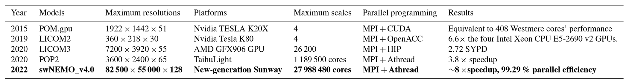
In the last few years, heterogeneous architectures (i.e., CPU + GPU, Vazhkudai et al., 2018; CPU + FPGA, Putnam et al., 2015; CPU + MIC, Liao et al., 2014; and MPE + CPE (computing processing element), Fu et al., 2016) have been widely applied to speed up model computation (Table 1). GPUs are increasingly important in high-performance computing due to their high-density computing. Using GPUs to accelerate computing speed shows great potential for the ocean and climate modeling. For example, based on mpiPOM, Xu et al. (2015) developed a POM (Princeton Ocean Model) GPU solution, which reduced power consumption by a factor of 6.8 times and achieved the equivalent performance of 408 Intel Westmere cores using four K20 GPUs (Xu et al., 2015). LICOM (LASG/IAP Climate system Ocean Model) was successfully ported and optimized to run on Nvidia and AMD GPUs, which showed great potential compared with CPUs (Jiang et al., 2019; Wang et al., 2021). Compared with GPUs, the results of ocean models published with FPGA are relatively few, and most are in the program porting stage.
On the platform of Sunway supercomputers, Zhang et al. (2020) and Zeng et al. (2020) studied the porting of the ocean component POP2 (Parallel Ocean Program version 2) and successfully scaled it to 1 million and 4 million cores, respectively, speeding up computation by a factor of 3 to 4. To use heterogeneous architectures, parallel programming of MPI + OpenMP/CUDA/OpenACC/Athread was developed to improve the parallel efficiency of the model using finer-grained parallelism (Afzal et al., 2017). The coordination between the master and slave cores (involving master–slave cores, slave–slave cores, memory bandwidth and register communication) is the key to parallel efficiency.
Due to the limitation of memory bandwidth, large-scale parallelism usually cannot maintain high efficiency (Lellouche et al., 2018; Ruston, 2019; Chassignet et al., 2019). The classic parallelization method is the “longitude–latitude 2D decomposition based on the MPI of OGCMs. To further improve parallelism, there are many efforts in parallel decomposition schemes and algorithm improvements of physical processes. To achieve better load balance, several decomposition schemes based on curve filling have been introduced in OGCMs (POP, Smith et al., 2010 and NEMO (Nucleus for European Modelling of the Ocean), Madec and the NEMO team, 2016). The parallel scale can reach O (100 km) in practice with a resolution of O (10 km) (Hu et al., 2013; Yang et al., 2021). However, due to the communication barrier, the large-scale parallel efficiency is still below 50 %. Therefore, we need to explore new schemes that can further improve the scalability to the next level. At the current stage, developing a large-scale parallel algorithm for the OGCMs is still in two-dimensional parallelism along with the longitudinal and latitudinal horizontal directions. Therefore, integrating the vertical direction in the three-dimensional parallelism scheme is still challenging.
As most emerging Exascale systems provide support for mixed-precision arithmetic, a mixed-precision computing scheme becomes an important step to reduce the computational and memory pressure further, as well as to improve the computing performance. However, due to the weak support of mixed precision from computer systems and the difficulty of balancing computing precision and simulation accuracy, many efforts are still at an early stage. Dawson and Düben (2017) used a reduced-precision emulator (RPE) to study the shallow water equation (SWE) model using mixed precision and found that the error caused by iterations with low precision can be solved by mixed precision. Then, based on the RPE, Tintó Prims et al. (2019) investigated the application of a mixed scheme of double precision (DP) and single precision (SP) on NEMO and verified the feasibility of half precision (HP) in the regional ocean model of ROMS (Regional Ocean Modeling System) (Tintó Prims et al., 2019). Previous studies have shown that mixed precision can improve computational efficiency. However, RPE can only verify the feasibility of mixed precision in theoretical models. The new-generation Sunway supercomputer, supporting HP, can lay a solid foundation for applying mixed-precision OGCMs.
The architecture of the new-generation of Sunway processors (SW26010 Pro) adopts a more advanced DDR4 compared with the original SW26010. It not only expands the capacity, but also greatly improves the direct memory access (DMA) bandwidth of the processor. The upgrade of the on-chip communication mechanism of many-core arrays makes the interconnection between CPEs more convenient and builds a more efficient global network on the entire supercomputer. The upgrade of these key technologies provides a solid foundation for the parallelization of OGCMs on the new generation of Sunway supercomputers. In this work, we design and implement a four-level parallel algorithm on three-dimensional space based on hardware–software co-design. We also resolve the problem of memory bandwidth through fine-grained data reuse technology, thus paving the way for the ultrahigh scalability of NEMO. Furthermore, based on Sunway's heterogeneous many-core architecture, a composite block algorithm and a dynamic scheduling algorithm based on LDCache are proposed to fully exploit the performance of many-core acceleration. Finally, half precision is introduced to further release the memory pressure of NEMO under simulation with ultrahigh resolution. We develop a highly scalable swNEMO_v4.0 based on the Nucleus for European Modelling of the Ocean version 4 (NEMO4) with the GYRE-PISCES benchmark (Madec and the NEMO team, 2016), which is the benchmark abbreviation of the Gyre Pelagic Interactions Scheme for Carbon and Ecosystem Studies, where PISCES is short for Pelagic Interactions Scheme for Carbon and Ecosystem Studies (Aumont et al., 2015). The resolution is equivalent to the horizontal resolution of 500 m on a global scale.
The following section briefly introduces the new generation of Sunway heterogeneous many-core supercomputing platforms. In Sect. 3, we briefly review the basics of NEMO4 and describe our optimization methods in detail. The performance results are discussed in Sect. 4, and Sect. 5 concludes this paper with discussions.
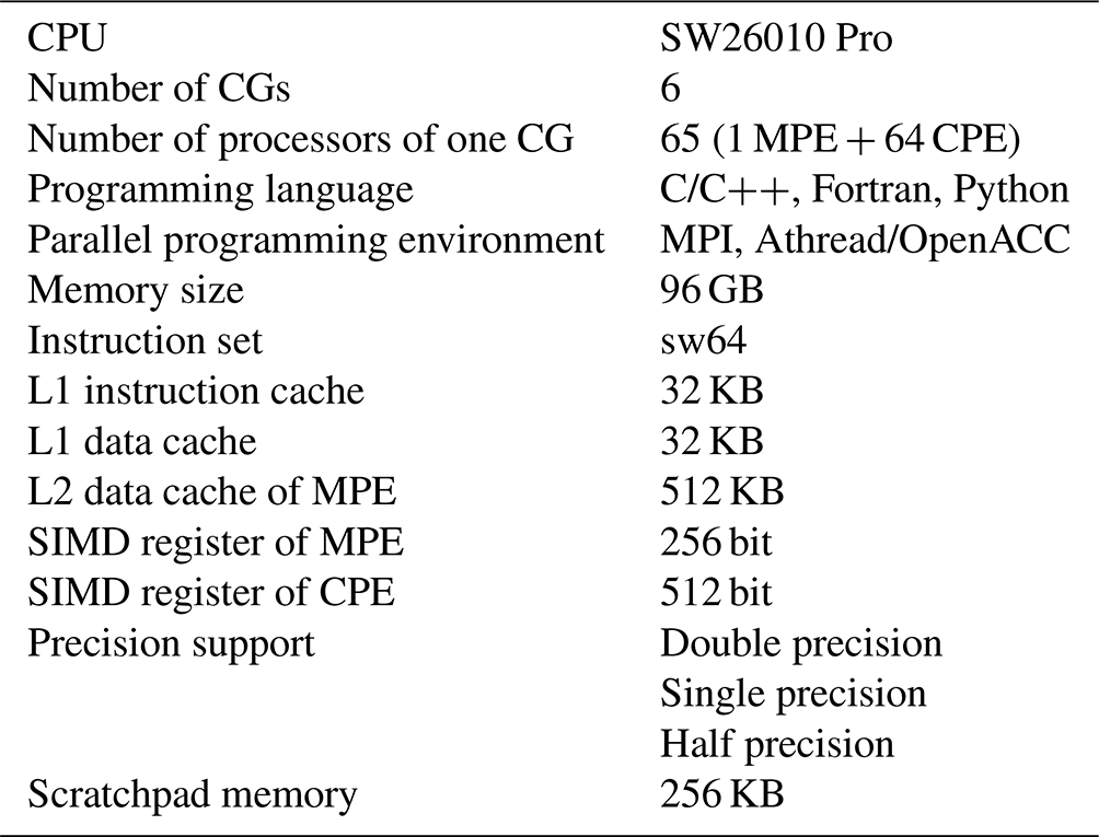
Succeeded by the architecture of Sunway TaihuLight, the new Sunway generation, as shown in Fig. 2, which is driven by SW26010 Pro (Table 2), consists of six core groups, with one management processing element (MPE) and one 8×8 computing processing element (CPE) cluster in each. The core groups are connected within the loop network. Data can be transferred between CPEs via remote memory access (RMA), which significantly increases the efficiency of CPE co-working.
CPE is also based on the SW64 instruction set, with the 512 bit single-instruction multiple-data (SIMD) vector, where double precision, single precision, half precision and integers are all supported. Furthermore, double and single precision share the same computation speed, whereas half precision performs twice faster. There are also a separate instruction cache and a scratchpad memory (SPM) in each CPE. The SPM allocates local data memory (LDM) for users, part of which can be set as a local data cache, automatically administrated by hardware. The data are transmitted between LDM and main memory via either direct memory access (DMA) or the general load and store instructions.
Table 2Basic information about SW26010 Pro. Note: CG refers to core group.

NEMO is a state-of-the-art modeling framework for research activities and forecasting services in the ocean and climate sciences developed in a sustainable way by a European consortium since 2008. It has been widely used in marine science, climate change studies, ocean forecasting systems and climate models. For ocean forecasting, NEMO has been applied by many operational forecasting systems, such as the Mercator Ocean monitoring and forecasting systems (Lellouche et al., 2018), as well as the ocean forecasting system in the National Marine Environmental Forecasting Center of China with a ∘ resolution (Wan, 2020). For the climate simulation and projections, approximately one-third of the climate models in the latest phase of the Coupled Model Intercomparison Project Phase 6 (CMIP6) (Eyring et al., 2016) use the ocean component models of NEMO. The breakthroughs made in this study are based on NEMO, and, thus, this work provides useful methods and ideas that can directly contribute to the NEMO community for optimizing their models and improving their simulation speeds.
Fully considering the characteristics of the three-dimensional spatial computation of OGCMs and the heterogeneous many-core architecture of the new-generation Sunway supercomputer, we develop a highly scalable NEMO4 named swNEMO_v4.0, with the following three major contributions based on the concepts of hardware–software co-design:
-
A highly efficient four-level parallelization framework is proposed for OGCMs to release a new level of parallelism along the column dimension that was originally not parallelism-friendly due to the computational dependency.
-
A raised many-core optimization method that uses an effective dynamic cache scheduling strategy utilizes the temporal and spatial locality of data effectively.
-
A multi-level mixed-precision optimization method that uses half, single and double precision is explored, which can effectively improve the computation performance while maintaining the same level of accuracy.
We then elaborate on the above algorithms in the following.
3.1 An adaptive four-level parallelization framework
To utilize the many heterogeneous cores of the new-generation Sunway supercomputer, the load of the expanded C-grid computation should be assigned in a balanced way. Considering the characteristics of the three-dimensional spatial computation of NEMO and the heterogeneous many-core architecture of a new-generation Sunway supercomputer, we propose an adaptive four-level parallel framework that can realize computation load dispatching among different levels. Figure 3 demonstrates our adaptive four-level parallel framework.
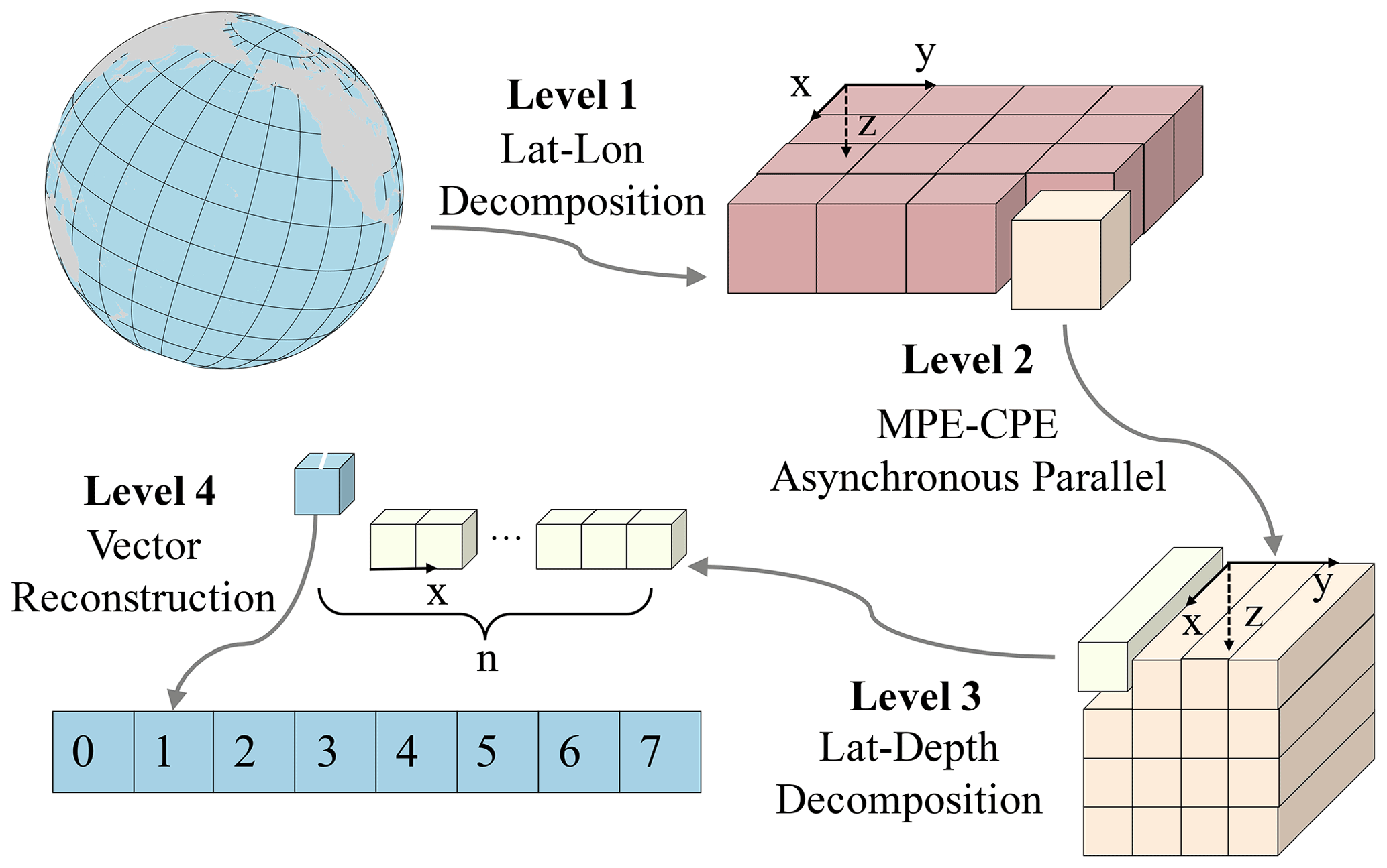
Figure 3The adaptive four-level parallel framework, where x, y and z axes indicate latitude, longitude and depth, respectively. Level 1 is the load-balanced longitude–latitude decomposition among MPEs, level 2 is the asynchronous parallel between a MPE and a CPE cluster, level 3 is the latitude–depth decomposition in a CPE clusters and level 4 is the vector reconstruction in a CPE.
3.1.1 Level 1: load-balanced longitude–latitude decomposition among MPEs
With land grids eliminated in NEMO, keeping the horizontal data in a traditional way benefits the load balance among processes. The variables are stored as 3-D arrays, and the x, y and z axes represent the longitude, latitude and depth, respectively. Since the scales of the x axis and y axis are considerably larger than the scale of the z axis, we decompose the data along the x axis and y axis and dispatch each data block to different MPI processes (first level of the four-level parallelization framework). Our major strategy is to guarantee that (a) the grid sizes of the subdomain in each process are similar, achieving a good load balance; and (b) the x axis and y axis dimension sizes are close to each other. The x axis and y axis of each process are the closest in all options, thus minimizing the halo areas that require communication among processes.
3.1.2 Level 2: asynchronous parallelization between a MPE and a CPE cluster
Gu et al. (2022) proposed a multi-level optimization method to use the heterogeneous architecture. In the first level of the method, they designed pre-communication, communication and post-communication in the code based on MPE–CPE asynchronous parallelism architecture. As the default barotropic solver in NEMO4 is an explicit method with a small time step, which is more accurate and more suitable for high resolution without a filter, instead of implicit or split-explicit methods (e.g., preconditioned conjugate gradients – PCGs), there is no global communication. Therefore, it is only necessary to update the information of the halo region between different processes. Moreover, in the explicit method, most boundary information exchanges are independent of the partition data in the process and can be used for asynchronous parallelization. So boundary data exchange can be parallelized aside from the computation. Considering that MPE is asynchronous with a CPE cluster, we propose an asynchronous parallelization design between the MPE and the CPE cluster using efficient DMA (second level of the four-level parallelization framework). The MPE is in charge of the boundary data exchange, I/O and a small amount of computation, while the CPE cluster performs the computation of most kernels. Such an asynchronous communication pattern can make full use of the asynchronous parallelism between the MPE and the CPE cluster, thus improving the parallel efficiency.
3.1.3 Level 3: “latitude–depth” decomposition in the CPE cluster
Furthermore, we design the third level of parallelism in the CPE cluster by utilizing the fine-grained data-sharing features within the CPE cluster, releasing a new level of parallelism along the column dimension that was originally not parallelism-friendly due to the computational dependency. RMA is a unique on-chip communication mechanism on the new-generation Sunway supercomputer, which enables high-speed communication among CPEs. We realize the latitude–depth decomposition with LDM and the data exchange with RMA. By utilizing the row and column communication features of RMA to achieve fine-grained data sharing among the CPE threads, we can accomplish an efficient parallelization on the column (i.e., the depth) dimension and release a new level of parallelism for the underlying hardware.
In the data structure of swNEMO, data items along the longitude axis are stored in a continuous way. Following such a memory layout, we divide the data block along the latitude and depth into smaller blocks and copy them into the LDM. More details are shown in Sect. 3.2.
3.1.4 Level 4: data layout reconstruction for vectorization
To further improve the computational efficiency within each CPE, we design the fourth level of parallelism for vectorization. SW26010 Pro has a 512 bit SIMD instruction set, one of which can compute eight double-precision digits simultaneously. To adapt our computation pattern for the SIMD instruction, we perform a data layout reconstruction to achieve the most suitable vectorization arrangement. Moreover, methods such as instruction rearrangement, branch prediction and cycle expansion are adopted to improve the execution efficiency of the instruction pipeline.
3.2 Performance optimization for the many-core architecture
3.2.1 A composite blocking algorithm based on RMA
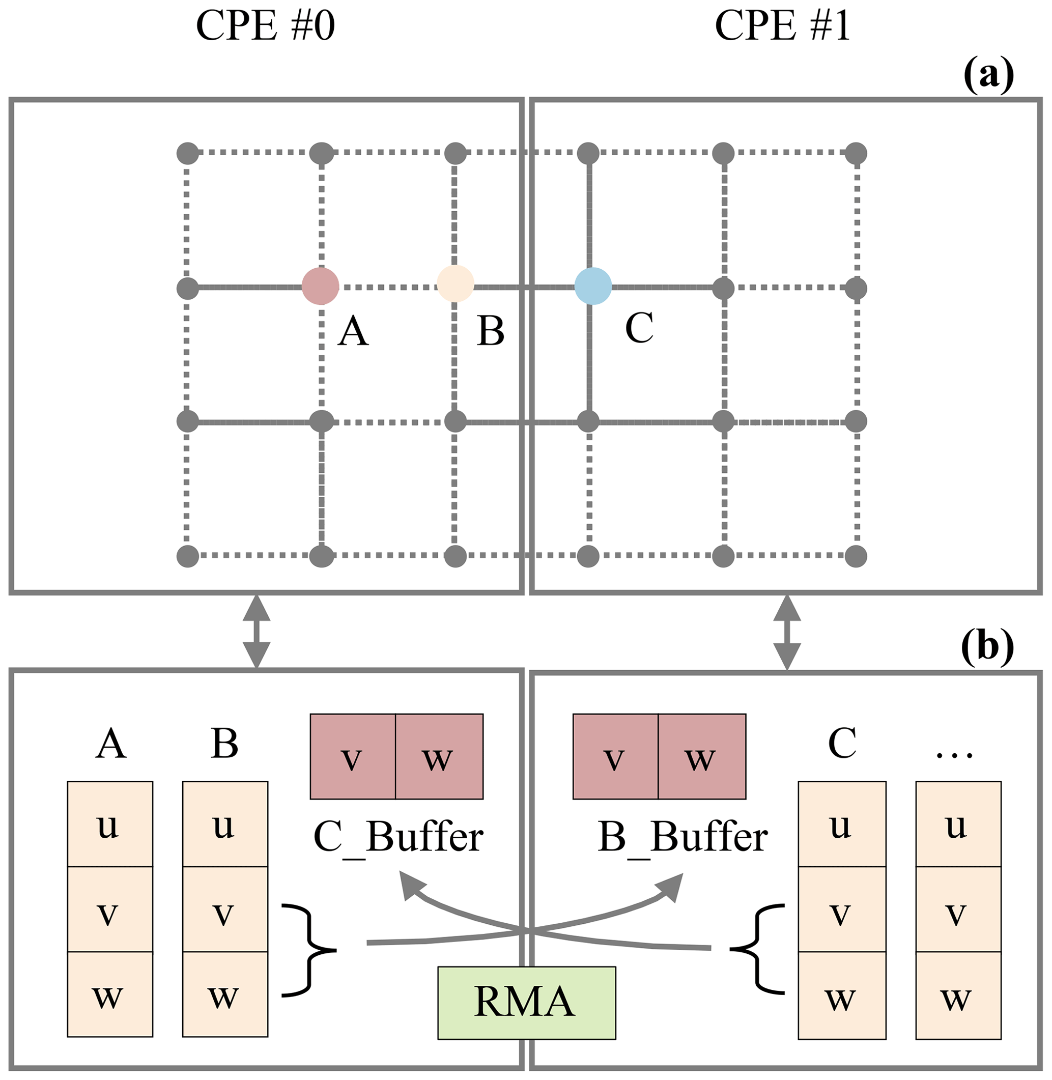
To further improve the parallel scale and efficiency, we implement the fine-grained latitude–depth decomposition. There are many stencils and temporal dependency computations existing in NEMO, which results in high demand for DMA bandwidth. A stencil computation is a class of algorithms that updates elements in a multidimensional grid based on neighboring values using a fixed pattern (hereafter called stencil). In a stencil operation, each point in a multidimensional grid is updated with the weighted contributions from a subset of its neighbors in both time and space, thereby representing the coefficients of the partial differential equation (PDE) for that data element. Therefore, we take advantage of the RMA provided by SW26010 Pro to relieve the pressure of the DMA bandwidth. RMA is an on-chip communication mechanism with superior bisection bandwidth within a CPE cluster. RMA enables direct remote LDM access among different CPEs within one CPE cluster. The efficient batch communication mechanism of RMA is highly adaptable for solving typical x pointer problems. For example, in the diffusion process of the tracer in NEMO, upstream points are needed for data exchange, which includes horizontal unidirectional grid information exchange (three-pointer stencil) and grid information exchange along with longitude and latitude directions (five-pointer stencil). Figure 4 represents the grid communication process between CPE #0 and CPE #1. Each point represents a multidimensional tensor composed of different variables that are irrelevant to each other. When updating A(u), variables v and w from the surrounding eight points are required to participate in the calculation. We first send v and w required by adjacent CPEs to the buffer in the corresponding CPEs while updating the local variables whose surrounding points are on the same CPE. After all the needed variables in the halo are transferred into the buffer, the remaining variables in the points located at the edge of the CPE can be updated.
Based on RMA, we design different parallel blocking algorithms for computing kernels with different characteristics to maintain an efficient performance in various application scenarios. In the following, α1, β1 and β2 are only the coefficient, f is the mathematical formula for the loop segment and x means the x axis (longitude axis) in the coordinate system.
-
Temporal dependency in computing along the z axis. We suppose is an original value of grid in the coordinate system (where the x axis is the most continuous one, and the z axis is the least), and is computed as follows:
where , and . In this equation, α1 and β1 are coefficients that indicate the linear characteristic of this mapping f. To fully utilize the DMA bandwidth, we decompose data along the y axis and send them into different CPEs. Then, continuous data along the x axis are copied into the LDM at one time.
-
Temporal dependency in computation along the y axis. In this case, the computation is as follows:
Here α2 and β2 are also coefficients that indicate the linear characteristic of this mapping f. Restricted by the size of the LDM, we decompose data along the z axis and then decompose data along the y axis into the proper size m and dispatch each data block into different CPEs as follows:
Therefore, blocks on the same z layer are dispatched to the same CPE one by one.
-
Nontemporal dependency in computation. In this case, we decompose the data along with the z axis and y axis. Due to the elaborate design of size (x), each block can be copied into LDM at once to reduce redundant halo transfer and improve the asynchronous parallel of stencil calculations.
To increase the utility of the RMA bandwidth, we pack the data before sending them for better utilization of the bandwidth in an aggregated manner. While sending, CPEs compute, and in this way, we can realize the overlap between RMA communication and computation and, thus, make efficient utilization of the bandwidth by reducing redundant DMA references. By utilizing RMA and the composite blocking strategy, for nontemporal-dependency and temporal-dependency computation, we finally achieve over 90 % effective utilization of the RMA bandwidth and over 80 % utilization of the DDR4 memory bandwidth. With such an efficient memory scheme, the average speedup of most computing kernels (comparing the performance of a CPE cluster to an MPE) can be up to 40 times.
3.2.2 A dynamic LDCache scheduling algorithm
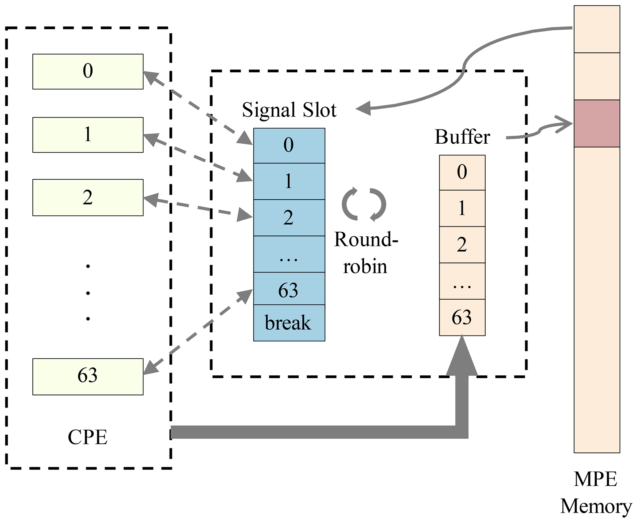
To access discrete data items in swNEMO, the traditional global load/global store (gld/gst) method becomes a major performance hindrance. LDCache, provided by SW26010 Pro, stores data with a cache_line of 256 bytes in CPE. In one CPE, LDM and LDCache share an SPM with a total capacity of 256 KB, and the size of LDM and LDCache can be manually adjusted. Since the amount of data required for a round of computation in different kernels in NEMO is varied, if the cache space is fixed, the utilization of the LDM becomes less efficient. Therefore, we design a dynamic LDCache scheduling algorithm that can realize efficient and fine-grained memory access. One feature of this algorithm is to dynamically adjust the size of LDCache to achieve a balance between LDM and LDCache. Furthermore, the algorithm has a time-division update technique since LDCache cannot guarantee data consistency with memory. We regularly update the stored data and eliminate the outdated data in the LDM simultaneously. As shown in Fig. 5, the data that need to be refreshed are packed on the CPE and sent to the designated buffer of the MPE. The MPE then uses the MPE–CPE message mechanism to find the buffers that need to be updated in a round-robin way and update them, while the CPE eliminates the corresponding data in the cache. By applying the dynamic LDCache scheduling algorithm with both an adjustable cache and a manual time-division update technique, we can improve the memory bandwidth utilization rate to approximately 88.7 % for DDR4, with a speedup of 88 times (comparing the performance of a CPE cluster to an MPE) for most computing kernels, which is a substantial improvement compared with the speedup of 5.1 times when using the traditional gld/gst method.
3.3 Mixed-precision optimization
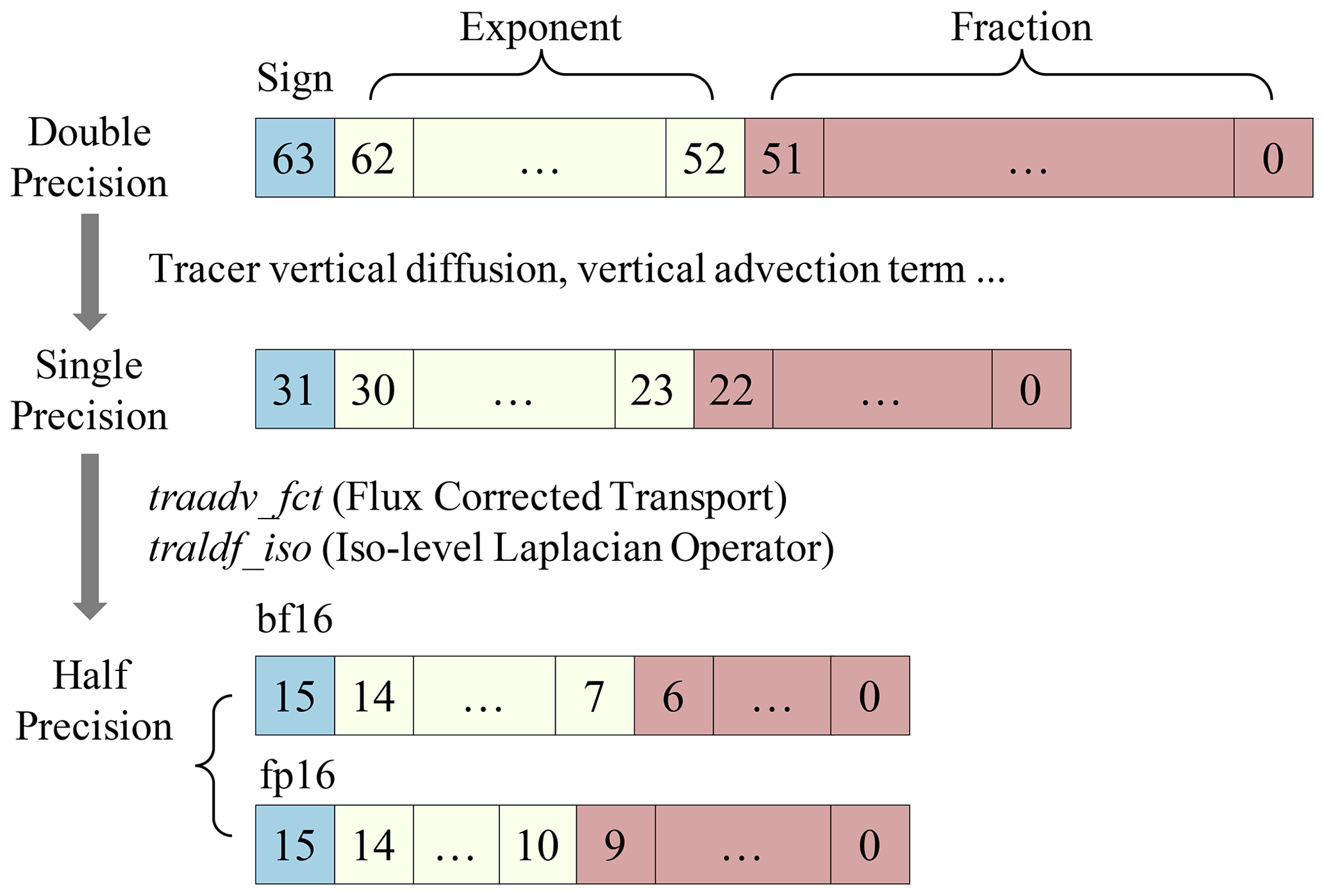
Because the NEMO, as one of the OGCMs, is memory-intensive, the memory bandwidth limits the computational efficiency of NEMO to a large extent. A reduced-precision method can be a promising solution. However, using low-precision data is a double-edged sword. On the one hand, it can effectively resolve the performance obstacles; on the other hand, the reduced precision brings errors and uncertainties. According to Dawson and Düben (2017), 95 % of NEMO variables support the single-precision floating-point format (SP). Therefore, we specifically reconstruct the data structure and introduce a new three-level mixed precision scheme in NEMO. To achieve a higher performance (Fig. 6), we reconstruct two “half-precision + single-precision” (HP + SP) computing kernels tracer_fct and tracer_iso of NEMO on CPE, which account for 50 % of the hotspot runtime in total. As HP is only supported on the CPEs of SW26010 Pro, we store HP data in the format of char or short types of memory on the MPE and use HP format to read them to LDM by DMA to ensure the correctness on the CPE.
By analyzing the calculation characteristics of NEMO, we find that the HP format subtracts operations between adjacent grids, which makes the final results diverge due to the round error of low precision. Therefore, a high-precision format must be used when calculating adjacent grids. Based on the above analysis in other calculations, we adopt the SP floating-point format for calculations between adjacent grids and the HP floating-point format with BF16 (consisting of 1 sign bit, 8 exponent bits and 7 mantissa bits). After optimization, we achieve a speedup of close to 2 times compared with NEMO using DP, while the maximum biases of temperature, salinity and velocity are within 0.05 % (figures not shown). Therefore, utilizing mixed precision can effectively increase the computational intensity and improve the scalability while maintaining the simulated accuracy of NEMO.
In order to validate the results of optimized swNEMO_v4.0, we carried out the perturbation experiments for the temperature results and analyzed the RMSZ (root-mean-square Z score) proposed by Baker et al. (2016). The experimental sample set can be represented as an ensemble , , where each sample Xm(j) represents a series of results at a given point j in all months. μ(j) and δ(j) represent the mean and standard deviations of this series at the given point j.
Since the experiment in this work is the ocean basin benchmark, it is not feasible to directly compare with observed values. Hence random disturbance conditions for the initial temperature are configured within the NEMO program. At the same time, we also selected 101 sets of data as experimental simulation results to validate the results of optimized NEMO_v4.0, of which 100 sets are temperature results with perturbation conditions, and the remaining one is the mixed-precision temperature field experimental results of swNEMO_v4.0.
At first, the perturbation coefficient is selected as O(10−14). However, we found that the RMSZ obtained by mixed-precision simulation was completely out of the shadow area formed by 100 simulations with double precision (Fig. 7a). Therefore, we increased the perturbation coefficient, and the mixed-precision Z score gradually approached the shadow area. We found that the disturbance had a greater influence in the first few years, then gradually decreased and tended to be stable after several years (Fig. 7a and b). As shown in Fig. 7b, when the perturbation coefficient is O(10−11), the Z score of mixed-precision simulation falls partially in the region formed by double-precision simulations. When the perturbation coefficient equals O(10−10), the Z score completely falls in the shadow area (Fig. 7c), which indicates that the effects of mixed precision are similar to these of the perturbation coefficient of O(10−10). It shows that the mixed-precision affects the results, but the effects are small (the perturbation coefficient is around O(10−10)) and can be accepted (Fig. 7c).

Figure 7RMSZ biases of the sea surface temperature in ensemble experiments (gray lines) with perturbation coefficient of (a) O(10−14), (b) O(10−11) and (c) O(10−10) and in the mixed-precision experiment (red line).
We choose the benchmark named GYRE-PISCES to test the swNEMO_v4.0 performance. The domain geometry is a closed rectangular basin on the β plane centered at ∼30∘ N and rotated by 45∘, 3180 km long, 2120 km wide and 4 km deep. The circulation is forced by analytical profiles of wind and buoyancy fluxes. This benchmark represents an idealized North Atlantic or North Pacific basin (Madec and the NEMO team, 2016). In addition, the east–west periodic conditions and the North Pole folding of the global ocean with a tripolar grid have a large impact on performance. Therefore, we activate the BENCH option to include these periodicity conditions and reproduce the communication pattern of the global ocean with a tripolar grid between two North Pole subdomains. It is equivalent to a global ocean with a tripolar grid with the same number of grid points from the perspective of computational cost and computational characteristics, although the physical meaning is limited. In the following content, the resolution of the benchmark is equivalent to that of the global ocean.
In this part, we have added a more specific description. We designed three groups of experiments with different resolutions of 2 km, 1 km and 500 m for strong expansibility. In addition, we also carried out weak-scalability experiments. The corresponding relationship among resolution, computing grid points and data scale of weak scalability can also be seen from the information in Table 3. The speedup is equal to the clock time in different scales divided by the baseline record of the minimum scale with 2 129 920 cores. For the weak-scalability analysis, we design the experiment with eight resolutions (Table 3). All experiments are run for 1 model day without I/O. We adopt the following methods to perform real-time statistics and floating points to ensure measurement accuracy.
-
For time statistics, we use two methods to proofread:
-
We use the MPI_Wtime() function provided by MPI to obtain the wall-clock time.
-
We use the assembly instructions to count the cycle time.
-
-
Similarly, two methods are used in the statistics of floating-point operations:
-
We use the loader to count the floating-point operation of the program when submitting the job.
-
We use performance interface functions to perform the program instrumentation to count the operations.
-
Table 3Eight different scales used in weak scalability, with the conversion between resolution in degrees and resolution in kilometers. The total number of computed grid points used in weak scalability is also shown.
4.1 Parallel-working performance on a many-core architecture
The cycle time and speedup ratio of the hotspots are shown in Fig. 8, where different parallel methods are applied for comparison with the original method. While the CPEs parallel method (level 3 of four-level parallel framework), which introduces all 64 slave kernels to help with acceleration, is 12 times faster than the original method, we find the master–slave asynchronous parallelization mode (MPE–CPE multilevel parallel, level 2 of four-level parallel framework) shows quite satisfying results with a speedup of 65 times. The four-level parallel framework fits well in Sunway architecture, and the master–slave asynchronous parallelization strategy combines data parallelism with task parallelism. By making great use of the Sunway architecture, this parallelization strategy overlaps the computation part with the communication and I/O part, thus considerably improving hotspot efficiency.

The Sunway architecture suggests storing data in slave kernels before further computation. Therefore, the performance of the many-core architecture is related to the actual amount of memory access, the bandwidth of DMA and the FLOPS performance of slave kernels. We assume the total amount of time of the hotspot part in slave kernels is represented by , where is the time cost of the actual floating-point operation in this part, and is the time cost of direct memory access. To speed up the many-core architecture, we can seek methods for both DMA optimization and floating-point operation optimization.
For stencil computation, due to the low ratio of computation to memory access, we have . We can minimize using computation–communication overlap, yet is related to the actual amount of memory access and the bandwidth of DMA , where BWDMA is the theoretical value of DMA bandwidth, and M is the total valid amount of memory access. In the real NEMO4 case, we have . Assuming the following equation holds true, , then the ratio of actual DMA bandwidth to theoretical bandwidth should be
The theoretical time cost of DMA when M is fixed is . Since is affected by the frequency and size of DMA, and hold. Therefore, we have
when or , α→1. The more the ratio of actual memory bandwidth to theoretical bandwidth approaches 1, the faster the whole architecture works and, thus, the better the performance becomes.
To analyze the performance of the algorithm mentioned in Sect. 3.2.1, we use five kernels to simulate the test, with grids on average per kernel. The five kernels are the most time-consuming chunks, which are only a fraction of the physical process. However, they are all specific implementations of Stencil computing. We calculate the average clock cycle of running one simulation, and the results are shown in Fig. 9 (see the Appendix for the detailed codes of Algorithms A1–A5), where the red bars are the original results, and the blue bars are the optimized results using this algorithm. It is clearly shown that the time cost is largely reduced via this method, as with the third kernel, the clock cycle is reduced from to s, which means the result becomes 70.9 times faster. Meanwhile, according to the simulation test, this algorithm raises the ratio of actual DMA bandwidth to theoretical bandwidth up to above 92 %, as shown in the third kernel, and even reaches the theoretical limit of 95 % as a whole.
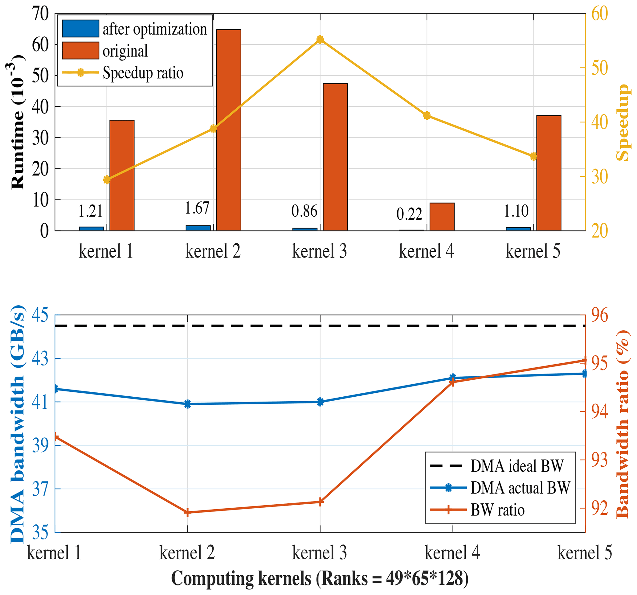
Figure 9The performance of the five-kernel simulation test and the five kernels are shown in the Appendix.
4.2 Mixed-precision optimization
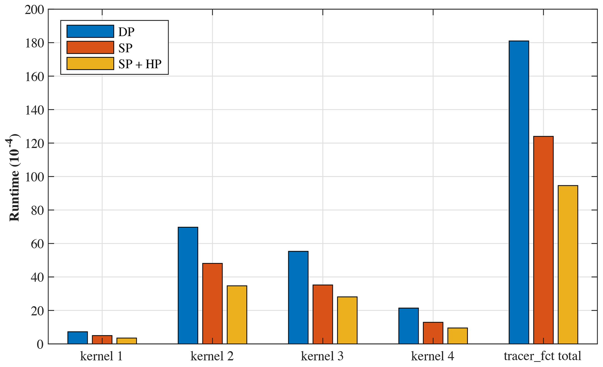
Introducing low-precision format data helps reduce memory use. Since the LDM in the slave kernel has limited storage, lowering the data precision could better use the given space and accelerate communication with the same actual DMA bandwidth. In terms of NEMO, due to its memory constraint, DMA data communication contributes to greater than 95 % of the total running time on the many-core architecture, and, as a result, we can enhance the overall performance by lowering the time cost of data communication. Focusing on tracer_fct in NEMO, we simulate a four-kernel test with a s grid on average per kernel, and the results, which include the optimizations of four-level parallelization framework and mixed-precision approaches, are shown in Fig. 10, where the red and orange bars represent the average wall time of SP and SP + HP in one simulation. Since NEMO is sensitive to precision, we cannot use HP only. We can see that the SP + HP method shortens the total time by half compared to the original DP method. To further explore this topic, we simulate another test comparing the bandwidth usage and the ratio in both SP and SP + HP precision, which is shown in Fig. 11. The result shows that both methods surpass the 90 % ratio threshold, with the fourth kernel performing best with a ratio of 95 %.

4.3 Strong scaling
Figure 12 shows the results of strong scaling. We conduct experiments with resolutions of 2 km, 1 km and 500 m, increasing the number of cores from 2 129 920 to 27 988 480. The numbers of grids at resolutions of 2 km, 1 km and 500 m are 24 002 × 16 002 × 128, 43 502 × 29 002 × 128 and 82 502 × 55 002 × 128, respectively. We set 2 129 920 cores as the baseline of strong scaling, and the final parallel efficiencies are 74.18 %, 83.40 % and 99.29 %, respectively.
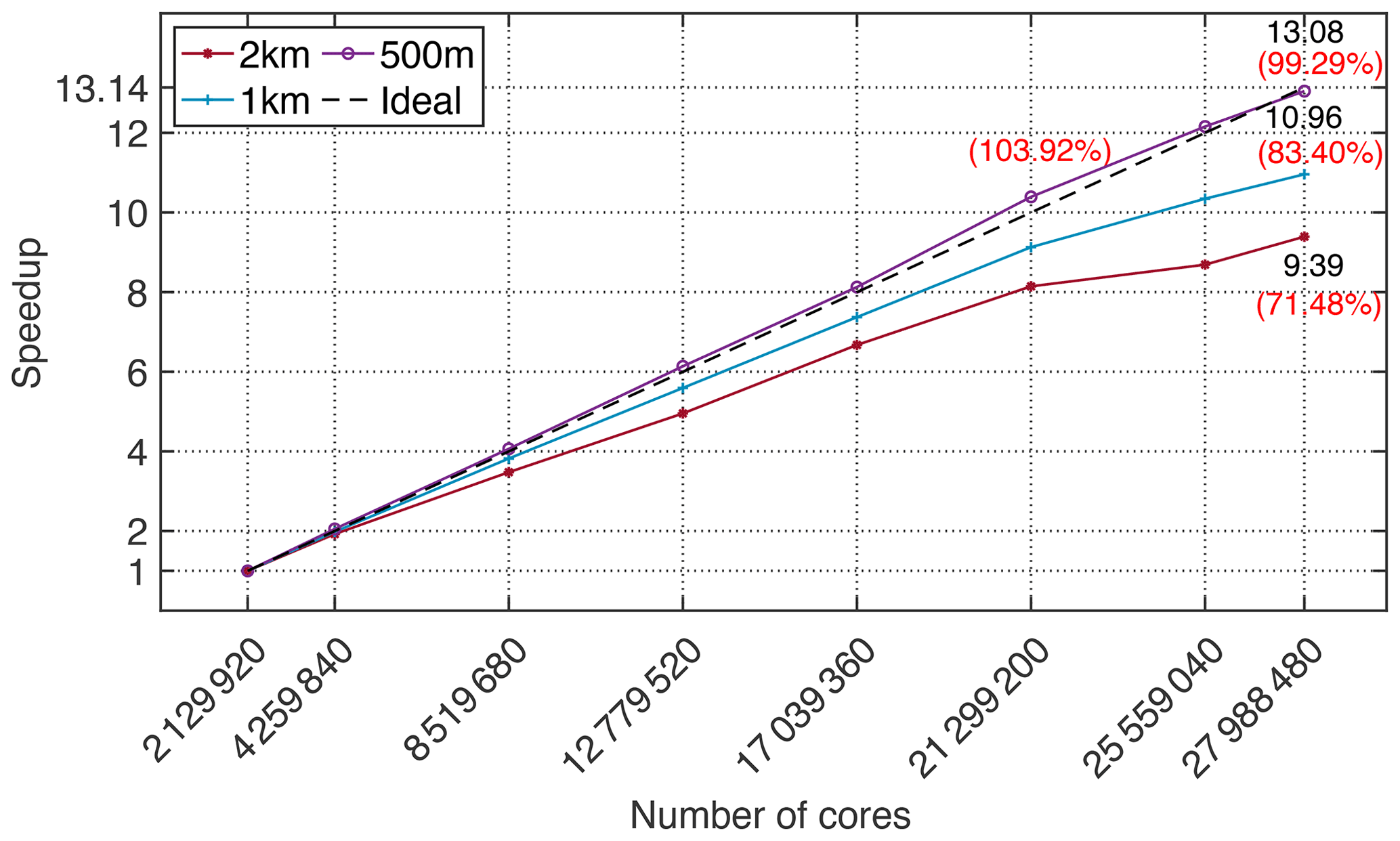
Figure 12The strong scalability results, scaling from 2 129 920 to 27 988 480 cores with 2 km, 1 km and 500 m resolutions.
When the number of cores is 2 129 920, the average computing task of each process (i.e., CG) is approximately 325 × 432, including a halo in the horizontal direction and 128 grids in the vertical direction. The mixed-precision optimization proposed in this paper considerably speeds up computations and reduces memory overhead. However, to guarantee the accuracy of the results, there are still some unavoidable double-precision floating-point arithmetics in the key steps in swNEMO_v4.0. During computing, the size of a four-dimensional variable with double precision has exceeded 1 GB. To maintain a reasonable efficiency of the memory system, we select 2 129 920 cores as the minimum available baseline.
For two-dimensional stencil computations, a grid with similar sizes of the x axis and y axis can effectively reduce the amount of communication and speed up the stencil computation. When the grid sizes of the x axis and the y axis are the same, the amount of communication touches the bottom. According to the four-level parallel architecture, the process-level task assignment does not involve grid partitioning in the vertical direction. For the strong scalability test, with a resolution of 500 m, the size of the horizontal grid is 82 502 × 55 002, and the size of the vertical grid is 128. When using 21 299 200 cores, the process division in the horizontal direction is 640 × 512. At this time, each process (i.e. CG) computes 128 × 108 grids, and the grid sizes of the x axis and the y axis of each process are the closest in all options. Therefore, the best parallel efficiency, 104 %, is achieved when the number of cores is 21 299 200.
In summary, the strong scalability of the three resolutions has always maintained high performance with 10 million cores, and the speedup is still nearly linear at an ultra-large scale. Using 27 988 480 cores, swNEMO_v4.0 achieves up to 99.29 % parallel efficiency with a high resolution of 500 m.
4.4 Weak scaling
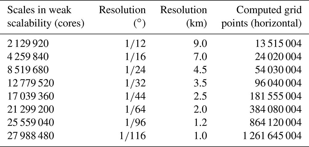
The choice of resolution of the GYRE needs to be followed with strict discipline. Therefore, to ensure that the workload in a single process is fixed, the number of grids of the x axis and y axis is proportional to the number of cores, and the automatic scheme of domain decomposition in swNEMO_v4.0 is replaced with a manual scheme at the same time, which is shown in Fig. 13 and Table 3.
As we build roofline models on NEMO, we find that when the horizontal grid surpasses 49×65 and the vertical grid surpasses 128, the computation efficiency of the floating point for a single core group performs the best. Therefore, our following experiments on weak scaling are conducted on a single core group with grid size each. Based on the above-mentioned principle, we choose resolutions of 9, 7, 4.5, 3.5, 2.5, 2.0, 1.2 and 1.0 km. According to the expansion of the workload of each process (i.e., CG), the number of cores increases from 299 520 to 27 988 480. With a resolution of 1.0 km, the total number of grids is 43 502 × 29 002 × 128. As shown in Fig. 13, the performance is stable with different resolutions, and the computation efficiency of the floating point is still 1.99 ‰ at a resolution of 1 km, which is very close to the baseline. The nearly linear trend indicates that the model has good weak scalability.
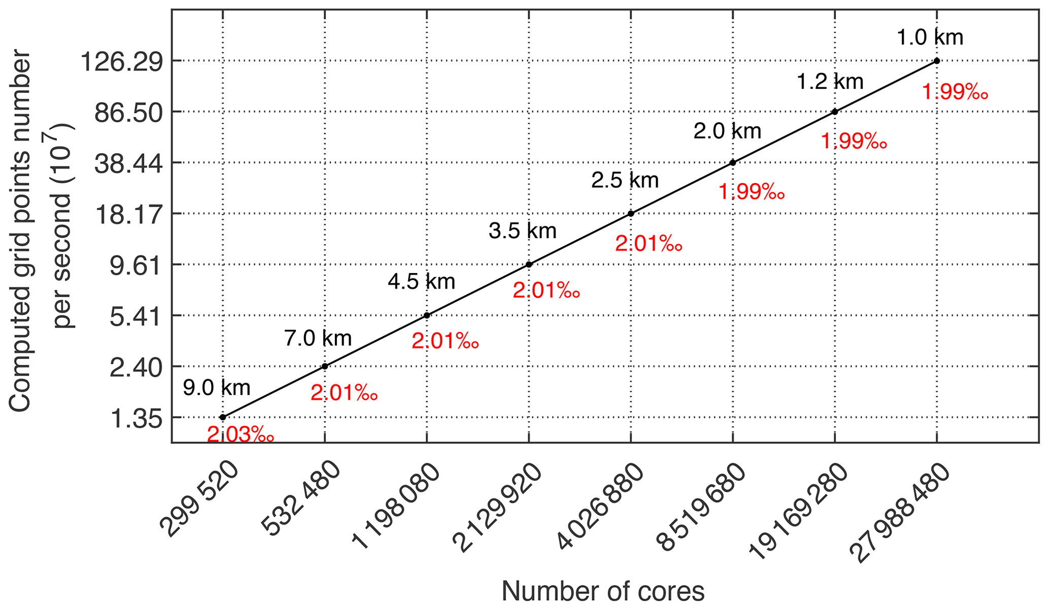
Figure 13The weak-scalability results, scaling from 299 520 to 27 988 480 cores with eight different resolutions.
4.5 Peak performance
Figure 14 shows the peak performance of swNEMO_v4.0 with a resolution of 1 km. When the total grid size is 43 502 × 29 002 × 128, the number of cores increases from 2 129 920 to 27 988 480. It is obvious that the optimal performance is 1.97 PFLOPS using 27 988 480 cores, and the performance of the optimized version is 10.25 times faster than that of the original version.

Figure 14The peak performance results for simulations with 1 km resolution. Numbers along the graph line are the peak performances for simulations with different cores. The peak performance with 27 988 480 cores reaches 1.973 PFLOPS.
In swNEMO_v4.0, we fully parallelize 70.58 % of the hotspots according to the performance profiling tools. The remaining 29.42 % of hotspots are mainly serial, which can hardly be parallelized. Therefore, mixed-precision optimization is used to optimize the serial part. According to Amdahl's law,
where the theoretical speedup is approximately by a factor of 6.8.
Combining the breakthroughs in an adaptive four-level parallelization design, CPE cluster optimization and mixed-precision optimization, the performance of our optimized version surpasses the theoretical values after further refactoring the code to reduce conditional judgment, instruction branching and the complexity of the code.
Additionally, as shown in Fig. 15, 1.43 SYPD (simulated years per day) with a resolution of 1 km using 27 988 480 cores is achieved, which is 7.53 times better compared with 0.19 SYPD of the original version, exceeding the ideal-performance upper bound.
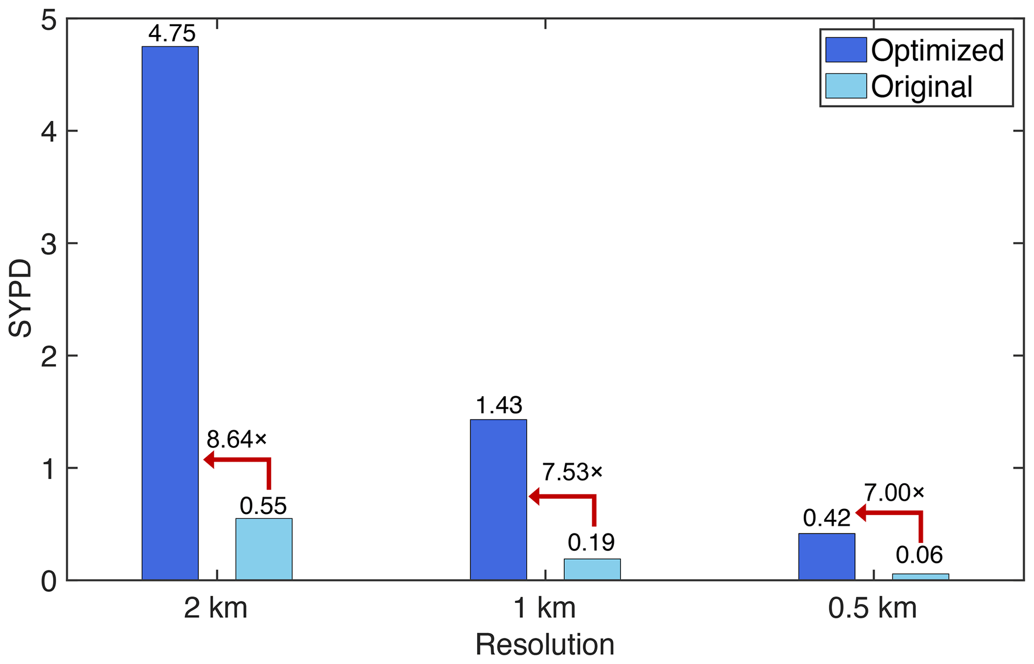
Figure 15The computing throughput results using 27 988 480 cores. The SYPD (simulated years per day) increases from 0.19 to 1.43 with the 1 km resolution. The optimized performance is 7.53 times better than that of the original version.
This paper presents a successful solution for global ocean simulations with ultrahigh resolution using NEMO on a new-generation Sunway supercomputer. Three breakthroughs, including an adaptive four-level parallelization design, many-core optimization and mixed-precision optimization, are designed and tested. The simulations achieve 71.48 %, 83.40 % and 99.29 % parallel efficiency with resolutions of 2 km, 1 km and 500 m using 27 988 480 cores, respectively.
Current resolutions of ocean models in ocean forecasting systems and climate models cannot resolve the mesoscale and sub-mesoscale eddies in the real ocean well, not to mention the other smaller-scale processes such as internal waves. However, these sub-mesoscale and small-scale processes are not only important to navigation safety in themselves, but also have notable influences on the large-scale simulations of the global/regional ocean and circulations through interacting with different scales. Improving resolution is one of the best ways to resolve these processes and improve simulations, forecasts and predictions. The highest resolution used in this study is 500 m, and this resolution can resolve the sub-mesoscale eddies well and partly resolve the internal waves, which are very important for the safety of offshore structures. Therefore, the breakthroughs made in this study make the direct simulations of these important sub-mesoscale and small-scale processes at the global scale possible. This will substantially improve the forecast and prediction accuracy of the ocean and climate while strongly supporting the key outcome of a predicted ocean of the UN Ocean Decade.
This study is conducted in the new generation of Sunway supercomputers. The breakthroughs in this paper, such as the four-level parallelization design and the method for efficient data transportation inside CPEs, provide novel ideas for other applications in this series of Sunway supercomputers. Moreover, the proposed new optimization approaches, such as a four-level parallel framework with longitude–latitude–depth decomposition, a multi-level mixed-precision optimization method that uses half, single and double precision, are the methods of general applicability. We test these optimization approaches in the NEMO, but these can be incorporated into other global/regional ocean general circulation models (e.g., MOM, POP and ROMS). Moreover, the optimizations on the stencil computation can be applied to any model with stencil computations.
High-resolution ocean simulations are crucial for navigation safety, weather forecasting and global climate change prediction. We believe that these approaches are also suitable for other OGCMs and supercomputers. In this paper, three innovative algorithms proposed based on the new generation of Sunway supercomputers provide an important reference for ultrahigh-resolution ocean circulation forecasting. However, only benchmarks are tested in the work, and real application data have not been used. In the future, we will build an ultrahigh-resolution ocean circulation forecasting model under real scenarios and conduct in-depth research to provide efficient solutions to predict ocean circulation and climate change accurately.
From the view of software and hardware co-design, the following should be focused on in the future. The first is the decomposition and load balance. For the model design, we should find the proper decomposition scheme to utilize the computer architecture fully. Besides the time dimension, solving an ocean general circulation model is a 3-dimensional problem, with longitude, latitude and depth. Usually, only the longitude–latitude domain is decomposed. In our work, driven by the RMA technology, we achieved the decomposition of the longitude–latitude–depth domain, which enables better large-scale scalability. Meanwhile, keeping a good load balance is also important for scalability. For the computer design, the RMA technology is a good example, which enables the decomposition of the longitude–latitude–depth domain. In other words, the high communication bandwidth between different cores or nodes will help achieve large-scale scalability. The second is communications. With the increasing processes used for model simulation, the ratio of communication time to computational time will increase. For the model design, the first thing is to avoid the global operator, such as ALLREDUCE and BCAST, which will take more time with an increase in processes. Otherwise, it will be the crucial bottleneck. Meanwhile, we also should pack the exchanged data between different processes as much as possible. For the computer design, the low latency will help in saving the communication time. The third is reduced precision. Our work's results demonstrate that there is a great potential to save computational time by incorporating the mixed double, single and half precision into the model. For the model design, we should understand the minimum computational precision requirements essential for successful ocean simulations and then revise or develop arithmetic. For the computer design, the support for half precision should be considered in the future.
Overall, the above are only several examples for further improving the performance of ocean modeling from perspectives of model development and computer design. Furthermore, other aspects such as I/O efficiency and the trade-off between precision and energy consumption should also be considered. Moreover, it should be noted that these suggestions are from different aspects of the model and computer development and need to be considered based on the software and hardware co-design ideology.
The following five chunks of code correspond to the five kernels stated in our previous experimental section. The codes listed below are exactly from NEMO for experimental validation.
Algorithm A1Â
Algorithm A2Â
Algorithm A3Â
Algorithm A4Â
Algorithm A5Â
The swNEMO_v4.0 source codes with the user manual are available at https://doi.org/10.5281/zenodo.5976033 (Ye et al., 2022a).
Processed data used in the production of figures in this paper are available via https://doi.org/10.5281/zenodo.6834799 (Ye et al., 2022b).
YY, ZS and SZ were involved in methodology, coding, numerical experiment, analysis and writing original draft preparation. YL, QS and BW were involved in algorithm description and validation. YL and WL were involved in the suggestion of the algorithm and numerical experiments. FQ and LW carried out the conceptualization, supervision, funding acquisition and editing. All authors discussed, read, edited and approved the article. All authors have read and agreed to the published version of the paper.
The contact author has declared that none of the authors has any competing interests.
Publisher’s note: Copernicus Publications remains neutral with regard to jurisdictional claims in published maps and institutional affiliations.
The authors would like to thank the two anonymous reviewers and the editor, for their constructive comments. All the numerical simulations were carried out at the Qingdao Supercomputing and Big Data Center.
This work is supported by the National Natural Science Foundation of China (grant nos. 41821004, U1806205, 42022042), the Marine S&T Fund of Shandong Province for Pilot National Laboratory for Marine Science and Technology (Qingdao) (grant no. 2022QNLM010202), the China–Korea Cooperation Project on Northwest Pacific Marine Ecosystem Simulation under the Climate Change and the CAS Interdisciplinary Innovation Team (grant no. JCTD-2020-12).
This paper was edited by Xiaomeng Huang and reviewed by two anonymous referees.
Afzal, A., Ansari, Z., Faizabadi, A. R., and Ramis, M.: Parallelization strategies for computational fluid dynamics software: state of the art review, Arch. Computat. Methods Eng., 24, 337–363, https://doi.org/10.1007/s11831-016-9165-4, 2017. a
Aumont, O., Ethé, C., Tagliabue, A., Bopp, L., and Gehlen, M.: PISCES-v2: an ocean biogeochemical model for carbon and ecosystem studies, Geosci. Model Dev., 8, 2465–2513, https://doi.org/10.5194/gmd-8-2465-2015, 2015. a
Baker, A. H., Hu, Y., Hammerling, D. M., Tseng, Y.-H., Xu, H., Huang, X., Bryan, F. O., and Yang, G.: Evaluating statistical consistency in the ocean model component of the Community Earth System Model (pyCECT v2.0), Geosci. Model Dev., 9, 2391–2406, https://doi.org/10.5194/gmd-9-2391-2016, 2016. a
Bryan, K.: A numerical method for the study of the circulation of the world ocean, J. Comput. Phys., 4, 347–376, 1969. a
Bryan, K. and Cox, M. D.: A numerical investigation of the oceanic general circulation, Tellus, 19, 54–80, https://doi.org/10.1111/j.2153-3490.1967.tb01459.x, 1967. a
Chassignet, E. P., LeSommer, J., and Wallcraft, A. J.: Generalcirculation models, in: Encyclopedia of Ocean Sciences, 3rd Edn., edited by: Cochran, K. J., Bokuniewicz, H. J., and Yager, P. L., Elsevier, 5, 486–490, https://doi.org/10.1016/B978-0-12-409548-9.11410-1, 2019. a, b, c
Dawson, A. and Düben, P. D.: rpe v5: an emulator for reduced floating-point precision in large numerical simulations, Geosci. Model Dev., 10, 2221–2230, https://doi.org/10.5194/gmd-10-2221-2017, 2017. a, b
Dong, J., Fox-Kemper, B., Zhang, H., and Dong, C.: The seasonality of submesoscale energy production, content, and cascade, Geophys. Res. Lett., 7, e2020GL087388, https://doi.org/10.1029/2020GL087388, 2020. a
Eyring, V., Bony, S., Meehl, G. A., Senior, C. A., Stevens, B., Stouffer, R. J., and Taylor, K. E.: Overview of the Coupled Model Intercomparison Project Phase 6 (CMIP6) experimental design and organization, Geosci. Model Dev., 9, 1937–1958, https://doi.org/10.5194/gmd-9-1937-2016, 2016. a
Fu, H., Liao, J., Yang, J., Wang, L., Song, Z., Huang, X., Yang, C., Xue, W., Liu, F., Qiao, F., Zhao, W., Yin, X., Hou, C., Zhang, C., Ge, W., Zhang, J., Wang, Y., Zhou, C., and Yang, G.: The sunway taihulight supercomputer: system and applications, Sci. China Inform. Sci., 59, 1–16, https://doi.org/10.1007/s11432-016-5588-7, 2016. a
Gu, J., Feng, F., Hao, X., Fang, T., Zhao, C., An, H., Chen, J., Xu, M., Li, J., Han, W., Yang, C., Li, F., and Chen, D.: Establishing a non-hydrostatic global atmospheric modeling system at 3-km horizontal resolution with aerosol feedbacks on the Sunway supercomputer of China, Sci. Bull., 67, 1170–1181, https://doi.org/10.1016/j.scib.2022.03.009, 2022. a
Hu, Y., Huang, X., Wang, X., Fu, H., Xu, S., Ruan, H., Xue, W., and Yang, G.: A scalable barotropic mode solver for the parallel ocean program, in: European Conference on Parallel Processing, edited by: Wolf, F., Mohr, B., and Mey, D., Springer, 739–750, https://doi.org/10.1007/978-3-642-40047-6_74, 2013. a
Jiang, J., Lin, P., Wang, J., Liu, H., Chi, X., Hao, H., Wang, Y., Wang, W., and Zhang, L.: Porting LASG/IAP climate system ocean model to GPUs using OpenAcc, IEEE Access, 7, 154490–154501, https://doi.org/10.1109/ACCESS.2019.2932443, 2019. a
Lellouche, J.-M., Greiner, E., Le Galloudec, O., Garric, G., Regnier, C., Drevillon, M., Benkiran, M., Testut, C.-E., Bourdalle-Badie, R., Gasparin, F., Hernandez, O., Levier, B., Drillet, Y., Remy, E., and Le Traon, P.-Y.: Recent updates to the Copernicus Marine Service global ocean monitoring and forecasting real-time ∘ high-resolution system, Ocean Sci., 14, 1093–1126, https://doi.org/10.5194/os-14-1093-2018, 2018. a, b, c
Liao, X., Xiao, L., Yang, C., and Lu, Y.: Milkyway-2 supercomputer: system and application, Front. Comput. Sci., 8, 345–356, https://doi.org/10.1007/s11704-014-3501-3, 2014. a
Madec, G. and the NEMO team: NEMO ocean engine, Zenodo, https://doi.org/10.5281/zenodo.3248739, 2016. a, b, c
Putnam, A., Caulfield, A. M., Chung, E. S., Chiou, D., Constantinides, K., Demme, J., Esmaeilzadeh, H., Fowers, J., Gopal, G. P., Gray, J., Haselman, M., Hauck, S., Heil, S., Hormati, A., Kim, J.-Y., Lanka, S., Larus, J., Peterson, E., Pope, S., Smith, A., Thong, J., Xiao, P. Y., and Burger, D.: A reconfigurable fabric for accelerating large-scale datacenter services, IEEE Micro., 35, 10–22, https://doi.org/10.1109/MM.2015.42, 2015. a
Qiu, B., Chen, S., Klein, P., Wang, J., Torres, H., Fu, L. L., and Menemenlis, D.: Seasonality in transition scale from balanced to unbalanced motions in the world ocean, J. Phys. Oceanogr., 48, 591–605, https://doi.org/10.1175/JPO-D-17-0169.1, 2018. a
Qiu, B., Chen, S., Klein, P., Torres, H., Wang, J., Fu, L. L., and Menemenlis, D.: Reconstructing upper-ocean vertical velocity field from sea surface height in the presence of unbalanced motion, J. Phys. Oceanogr., 50, 55–79, https://doi.org/10.1175/JPO-D-19-0172.1, 2020. a
Rocha, C. B., Gille, S. T., Chereskin, T. K., and Menemenlis, D.: Seasonality of submesoscale dynamics in the kuroshio extension, Geophys. Res. Lett., 43, 11–304, https://doi.org/10.1002/2016GL071349, 2016. a
Ruston, B.: Validation test report for the dtic, https://apps.dtic.mil/sti/pdfs/AD1090615.pdf (last access: 13 July 2022), 2019. a
Smith, R., Jones, P., Briegleb, B.,Bryan, F., Danabasoglu, G., Dennis, J., Dukowicz, J., Eden, C., Fox-Kemper, B., Gent, P., Hecht, M., Jayne, S., Jochum, M., Large, W., Lindsay, K., Maltrud, M., Norton, N., Peacock, S., Vertenstein, M., and Yeager, S.: The parallel ocean program (pop) reference manual ocean component of the community climate system model (ccsm) and community earth system model (cesm), LAUR-01853, 141, 1–140, https://www.cesm.ucar.edu/models/cesm1.0/pop2/doc/sci/POPRefManual.pdf (last access: 13 July 2022), 2010. a
Tintó Prims, O., Acosta, M. C., Moore, A. M., Castrillo, M., Serradell, K., Cortés, A., and Doblas-Reyes, F. J.: How to use mixed precision in ocean models: exploring a potential reduction of numerical precision in NEMO 4.0 and ROMS 3.6, Geosci. Model Dev., 12, 3135–3148, https://doi.org/10.5194/gmd-12-3135-2019, 2019. a, b
Vazhkudai, S. S., deSupinski, B. R., Bland, A. S., Geist, A., Sexton, J., Kahle, J., Zimmer, C. J., Atchley, S., Oral, S., Maxwell, D. E., Vergara Larrea, V. G., Bertsch, A., Goldstone, R., Joubert, W., Chambreau, C., Appelhans, D., Blackmore, R., Casses, B., Chochia, G., Davision, G., Ezell, M. A., Gooding, T., Gonsiorowski, E., Grinberg, L., Hanson, B., Hartner, B., Karlin, I., Leininger, M. L., Leverman, D., Marroquin, C., Moody, A., Ohmacht, M., Pankajakshan, R., Pizzano, F., Rogers, J. H., Rosenburg, B., Schmidt, D., Shankar, M., Wang, F., Watson, P., Walkup, B., Weems, L. D., and Yin, J.: The design, deployment, and evaluation of the coral pre-exascale systems, in: SC18: International Conference for High Performance Computing, Networking, Storage and Analysis, IEEE, 661–672, https://doi.org/10.1109/SC.2018.00055, 2018. a
Viglione, G. A., Thompson, A. F., Flexas, M. M., Sprintall, J., and Swart, S.: Abrupt transitions in submesoscale structure in southern drake passage: Glider observations and model results, J. Phys. Oceanogr., 48, 2011–2027, https://doi.org/10.1175/JPO-D-17-0192.1, 2018. a
Wan, L.: The high resolution global ocean forecasting system in the nmefc and its intercomparison with the godae oceanview iv-tt class 4 metrics, https://www.godae.org/$∼$godae-data/OceanView/Events/DA-OSEval-TT-2017/2.3-NMEFC-High-Resolution-Global-Ocean-Forecasting-System-and-Validation_v3.pdf (last access: 13 July 2022), 2020. a
Wang, P., Jiang, J., Lin, P., Ding, M., Wei, J., Zhang, F., Zhao, L., Li, Y., Yu, Z., Zheng, W., Yu, Y., Chi, X., and Liu, H.: The GPU version of LASG/IAP Climate System Ocean Model version 3 (LICOM3) under the heterogeneous-compute interface for portability (HIP) framework and its large-scale application , Geosci. Model Dev., 14, 2781–2799, https://doi.org/10.5194/gmd-14-2781-2021, 2021. a
Xu, S., Huang, X., Oey, L.-Y., Xu, F., Fu, H., Zhang, Y., and Yang, G.: POM.gpu-v1.0: a GPU-based Princeton Ocean Model, Geosci. Model Dev., 8, 2815–2827, https://doi.org/10.5194/gmd-8-2815-2015, 2015. a, b
Yang, X., Zhou, S., Zhou, S., Song, Z., and Liu, W.: A barotropic solver for high-resolution ocean general circulation models, J. Mar. Sci. Eng., 9, 421, https://doi.org/10.3390/jmse9040421, 2021. a
Ye, Y., Song, Z., Zhou, S., Liu, Y., Shu, Q., Wang, B., Liu, W., Qiao, F., and Wang, L.: swNEMO(4.0), Zenodo [code], https://doi.org/10.5281/zenodo.5976033, 2022a. a
Ye, Y., Song, Z., Zhou, S., Liu, Y., Shu, Q., Wang, B., Liu, W., Qiao, F., and Wang, L.: Data for swNEMO_v4.0 in GMD, Zenodo [data set], https://doi.org/10.5281/zenodo.6834799, 2022b. a
Zeng, Y., Wang, L., Zhang, J., Zhu, G., Zhuang, Y., and Guo, Q.: Redistributing and optimizing high-resolution ocean model pop2 to million sunway cores, in: International Conference on Algorithms and Architectures for Parallel Processing, edited by: Qiu, M., Springer, https://doi.org/10.1007/978-3-030-60245-1_19, 2020. a
Zhang, S., Fu, H., Wu, L., Li, Y., Wang, H., Zeng, Y., Duan, X., Wan, W., Wang, L., Zhuang, Y., Meng, H., Xu, K., Xu, P., Gan, L., Liu, Z., Wu, S., Chen, Y., Yu, H., Shi, S., Wang, L., Xu, S., Xue, W., Liu, W., Guo, Q., Zhang, J., Zhu, G., Tu, Y., Edwards, J., Baker, A., Yong, J., Yuan, M., Yu, Y., Zhang, Q., Liu, Z., Li, M., Jia, D., Yang, G., Wei, Z., Pan, J., Chang, P., Danabasoglu, G., Yeager, S., Rosenbloom, N., and Guo, Y.: Optimizing high-resolution Community Earth System Model on a heterogeneous many-core supercomputing platform, Geosci. Model Dev., 13, 4809–4829, https://doi.org/10.5194/gmd-13-4809-2020, 2020. a
- Abstract
- Introduction
- The new-generation heterogeneous many-core supercomputing platform and NEMO4
- Porting and optimizing NEMO4
- Performance results
- Conclusions and discussions
- Appendix A:âSupplementary code in Fortran format
- Code availability
- Data availability
- Author contributions
- Competing interests
- Disclaimer
- Acknowledgements
- Financial support
- Review statement
- References