the Creative Commons Attribution 4.0 License.
the Creative Commons Attribution 4.0 License.
 | 22 Jul 2022
Use of genetic algorithms for ocean model parameter optimisation: a case study using PISCES-v2_RC for North Atlantic particulate organic carbon
Marcus Falls
Raffaele Bernardello
Miguel Castrillo
Mario Acosta
Joan Llort
When working with Earth system models, a considerable challenge that arises is the need to establish the set of parameter values that ensure the optimal model performance in terms of how they reflect real-world observed data. Given that each additional parameter under investigation increases the dimensional space of the problem by one, simple brute-force sensitivity tests can quickly become too computationally strenuous. In addition, the complexity of the model and interactions between parameters mean that testing them on an individual basis has the potential to miss key information. In this work, we address these challenges by developing a biased random key genetic algorithm (BRKGA) able to estimate model parameters. This method is tested using the one-dimensional configuration of PISCES-v2_RC, the biogeochemical component of NEMO4 v4.0.1 (Nucleus for European Modelling of the Ocean version 4), a global ocean model. A test case of particulate organic carbon (POC) in the North Atlantic down to 1000 m depth is examined, using observed data obtained from autonomous biogeochemical Argo floats. In this case, two sets of tests are run, namely one where each of the model outputs are compared to the model outputs with default settings and another where they are compared with three sets of observed data from their respective regions, which is followed by a cross-reference of the results. The results of these analyses provide evidence that this approach is robust and consistent and also that it provides an indication of the sensitivity of parameters on variables of interest. Given the deviation in the optimal set of parameters from the default, further analyses using observed data in other locations are recommended to establish the validity of the results obtained.
- Article
(5079 KB) - Full-text XML
- BibTeX
- EndNote


The field of Earth science has garnered much interest in recent years due to anthropogenic-driven climate change and the increasing urgency to implement policies and technologies to mitigate its effects. As a result, Earth system models (ESMs) have become a fundamental tool for studying the impact of shifting climate dynamics and global biogeochemical cycles (Eyring et al., 2016; Anav et al., 2013; Flato, 2011). Driven by the necessity of policymakers to have increasingly reliable future climate projections, ESMs are being continuously developed, resulting in highly complex and computationally demanding tools. Nevertheless, climate projections produced by ESMs are still hampered by both technical limitations and a lack of knowledge of important processes (Seferian et al., 2020; Henson et al., 2022). Particularly, the representation of the global carbon cycle, specifically ocean biogeochemistry, suffers from many uncertainties. Moreover, the drive for realistic physical processes is pushing ESMs towards a higher spatial resolution, making the cost of calibrating the ocean biogeochemical component (and other components of ESMs) unsustainable (Galbraith et al., 2015; Kriest et al., 2020). Thus, there is a vital need for novel solutions that allow the optimisation of such components in a cost-effective way in order to provide critical analyses of the evolution of the climate and answer key societal questions in relation to it (Palmer, 1999, 2014).
The tool presented here can be applied to any ESM component, although this work focuses on ocean biogeochemistry because of the many unconstrained parameters that are usually needed to numerically represent this realm of the Earth system. In particular, we focus on key biogeochemical processes that contribute to the oceans' capacity to absorb carbon dioxide from the atmosphere and potentially store it. These processes, usually referred to as the biological carbon pump, are dominated by the vertical transport of organic matter from the surface of the ocean to deeper layers (Boyd et al., 2019). This organic matter is exported mostly in the form of detrital particles, which are partly decomposed back to inorganic carbon and nutrients by bacteria as they sink, and are also transformed by zooplankton. The interplay between biological processes and sinking determines how long this carbon will be stored in the ocean. Given that the oceans have absorbed around 30 % of the carbon dioxide released by human activity since preindustrial times (Gruber et al., 2019), constraining uncertainties in these biogeochemical processes is crucial to predict the future evolution of the climate system. However, their representation in models is still a challenge, in particular in the mesopelagic layer that extends between the bottom of the sunlit upper ocean and 1000 m, where around 90 % of detrital matter degradation takes place (Burd et al., 2010; Henson et al., 2022).
Ocean biogeochemistry models (OBGCMs) simplify the complexity of the real world by representing biological processes with empirical functions (Fasham et al., 1990), which are parameterised based on laboratory experiments (Pahlow et al., 2013) and sparse field measurements (Friedrichs et al., 2007; Aumont et al., 2015). Therefore, it is likely that model parameterisations do not reflect the complexity and diversity present in our oceans.
In the effort to achieve simple yet universally applicable models, parameter optimisation (PO) techniques are a key tool, as they provide an objective means to find a model parameter set that produces outputs that match well with observed datasets. However, PO (often referred to as tuning) has traditionally been a rather subjective process, in that the model developers choose the best parameter sets from a somewhat comprehensive array of alternative model runs. Such subjective optimisation often relied on sensitivity analyses, whereby the variations in model output variables, and their skill, were quantified by perturbing one parameter at a time. Given the high computational cost of 3D OBGCM simulations, subjective criteria are still widely used to optimise OBGCMs. A promising alternative is to perform PO using one-dimensional (1D) model configurations, which deal only with local sources and sinks and vertical fluxes along the water column (Fasham et al., 1990; Friedrichs et al., 2007; Bagniewski et al., 2011; Ayata et al., 2013). Optimising OBGCMs in 1D is advantageous as it enables a thorough exploration of the parameter space at a reduced computing cost.
Attempting to constrain parameters using optimisation techniques can be difficult in situations of inadequate data or computing power (Matear, 1995; Fennel et al., 2000). However, in recent years, this approach has become more viable within the scientific community due to improvements in high-performance computing (HPC) techniques that efficiently exploit the parallelism of supercomputers (Casanova et al., 2011; Broekema and Bal, 2012). These advances facilitate the running of multiple simulations in parallel, opening the way to efficiently apply PO methods to better understand and improve model accuracy. For instance, genetic algorithms (GAs), a particular type of optimisation technique, can and have been applied to many global search problems and have also started to be used to optimise numerical weather models (Oana and Spataru, 2016) and OBGCMs (Ayata et al., 2013; Ward et al., 2010; Shu et al., 2022). Another approach is the training of surrogate models (e.g. using neural networks) from a large set of simulations, enabling global sensitivity analyses at reduced computational cost, as done by the Uranie tool (Gaudier, 2010). What these different algorithms have in common is the fact that they are based on iterative processes traversing a search space by applying operations on the candidate solutions with the purpose of finding a global optimum. Candidate solutions are evaluated by a fitness function to evaluate their performance in the solution domain.
This paper documents the application of a genetic algorithm to determine an ideal set of parameters that accurately simulate the behaviour of the biogeochemical component (PISCES-v2_RC) of an ocean model. The overall aim of this investigation is to demonstrate that using computational intelligence techniques, a biased random key genetic algorithm (BRKGA) in our case, for parameter estimation in Earth system models is an effective approach and to explore, via a BRKGA, how this can be implemented. We also describe how to implement a BRKGA and how to embed it in a state-of-the-art ocean model using a workflow manager (Manubens-Gil et al., 2016).
This section outlines the main methods used in this investigation. A test case of particulate organic carbon (POC) in the North Atlantic down to 1000 m is used. The observed data, explained in detail in Sect. 2.1, are obtained from autonomous ocean Argo floats. The model tested is the one-dimensional (depth) configuration of the ocean biogeochemical model PISCES-v2_RC (Aumont et al., 2015, 2017), a component of NEMO4 v4.0.1 (Nucleus for European Modelling of the Ocean version 4), as outlined in Sect. 2.2.
The type of GA used is BRKGA (Goncalves and Resende, 2011). The outline of this method, including the crossover, is described in Sect. 2.3. We use the workflow manager Autosubmit (Manubens-Gil et al., 2016; Uruchi et al., 2021) to create a workflow that facilitates the various steps of the algorithm, as outlined in Sect. 2.4.
This paper outlines two test case experiments in which the reference data are an output of a simulation with default parameters, another three in which the reference data are observed data from three locations in the North Atlantic, and, last, a set of cross-experiments. Section 2.5 outlines the details of these experiments.
2.1 Biogeochemical data
Our investigation focuses on the vertical profiles of POC in the Labrador Sea region of the North Atlantic subpolar gyre. The observed data were acquired by Argo floats deployed in the context of the international Argo programme (Roemmich et al., 2019). Argo floats are autonomous drifting floats fitted with sensors that provide real-time updates of ocean data. Over regular intervals, each float rises from its drifting depth of 1000 m to the surface, taking measurements in the process. When it reaches the surface, it transmits the measurements. Initially, the Argo programme focused on observing salinity and temperature but, more recently, has included biogeochemical measurements (Claustre et al., 2020). Our investigation focuses on the data of two floats deployed by the project remOcean and identified by World Meteorological Organisation numbers 6901486 and 6901527. These floats took measurements every 1–3 d during times of high biological activity (i.e. phytoplankton blooms) and every 10 d for the rest of the year.
To enable comparison between biogeochemical (BGC)–Argo data and model simulations, we developed a framework that is described in detail in the companion paper by Galí et al. (2022). Briefly, particulate backscattering measurements acquired by Argo floats were converted to POC using depth-dependent empirical conversion factors and separated into two size fractions, small POC (SPOC) and large POC (LPOC), following Briggs et al. (2020). SPOC corresponds to particles smaller than ca. 100 µm that are suspended or sink slowly, approximately less than 10 m d−1, and LPOC corresponds to particles larger than 100 µm whose sinking rates are typically of the order of several tens or hundreds of metres per day. For each float, we selected one or more periods of 1 year that were deemed representative of the annual cycle in our study region.
-
LAB1 – float 6901527, year 2016, and −46.2∘ W, 57.2∘ N.
-
LAB2 – float 6901527, year 2014, and −54.9∘ W, 57.1∘ N.
-
LAB3 – float 6901486, year 2015, and −50.3∘ W, 56.3∘ N.
Finally, we matched the trajectory of the float on a given year to the NEMO model ORCA1 grid (ca. 1∘ horizontal resolution), and chose the ORCA1 grid cell with the best correspondence between the mixed layer depth observed by the float and that simulated by NEMO (see the next section), hence treating the float as if it sampled a fixed location.
2.2 PISCES 1D and parameters
PISCES-v2 (Aumont et al., 2015) is an OBGCM of intermediate complexity that represents the cycles of the main inorganic nutrients (N, P, Si, and Fe), carbonate chemistry, and organic matter compartments, including phytoplankton and zooplankton organisms (with two size classes each), dissolved organic matter, and particulate organic matter, making up 24 prognostic variables or tracers in total. Here we use a model version, PISCES-v2_RC, that incorporates the POC reactivity continuum parameterisation (Aumont et al., 2017). This model version is included as the OBGCM component of NEMO4 v4.0.1 (Madec et al., 2022) and will hereafter be referred to as PISCES.
In PISCES, detrital POC is represented by two tracers, i.e. POC for detritus smaller than 100 µm and GOC for detritus larger than 100 µm. To avoid confusion between PISCES tracers and the term POC, used here as a generic concept and to refer to observations, PISCES tracer names are italicised. It is important to note that total POC as sampled in situ is made up of detrital matter and living biomass. Therefore, the correspondence between PISCES tracers and observations must be established. Here we define SPOC as the sum of the PISCES tracers for nanophytoplankton (PHY), microphytoplankton (PHY2), microzooplankton (ZOO) and small detritus (POC), and LPOC as the sum of large detritus (GOC) and mesozooplankton (ZOO2). These idealised fractions show good correspondence with those determined from BGC–Argo data (Galí et al., 2022). It is important to keep in mind that detrital POC is a variable proportion of total POC, which generally increases with depth. In the mesopelagic, detrital POC represents around 70 % of total POC globally with the default PISCES parameterisation (Table 3 in Galí et al., 2022).
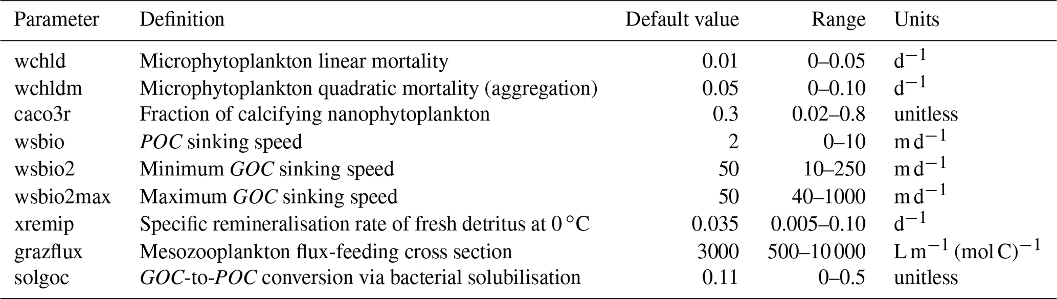
Our study focuses on nine PISCES parameters (Table 1) expected to strongly influence mesopelagic POC dynamics according to model equations (Aumont et al., 2015, 2017) and preliminary analyses (Appendix A and B). These parameters control POC formation in the surface productive layer through microphytoplankton mortality, gravitational POC fluxes, POC degradation rates, and interception and fragmentation of sinking POC by mesopelagic zooplankton. Preliminary tests also included the parameters unass and unass2, which determine POC production from the unassimilated fraction of phytoplankton biomass ingested by zooplankton. However, they were eventually excluded because these parameters have a strong impact on upper ocean (epipelagic) ecosystem dynamics, which are beyond the scope of our study.
Table 1Definitions of the PISCES parameters included in the optimisation experiments, along with their default values, optimisation ranges, and units.
This investigation uses PISCES configured for one spatial dimension (1D) and to run offline (Galí et al., 2022). The 1D configuration has the same vertical levels as the 3D configuration (in our setup, 75 levels of gradually increasing thickness – L75 vertical grid), but the horizontal grid is reduced to an idealised domain of 3×3 cells. In this configuration, tracer concentrations change over the temporal and vertical dimensions as a result of local sources and sinks, vertical diffusion, particle sinking through the water column, and fluxes at the ocean–atmosphere boundary. PISCES computes the sources and sinks and the gravitational sinking of detrital particles at each biological time step (here set to 45 min, which is one-fourth of the NEMO4 v4.0.1 time step). Then, the NEMO component TOP (Tracers in the Ocean Paradigm) calculates vertical diffusion using dynamical fields, which are precalculated in a previous NEMO run, with a time step of 3 h. The 1D configuration does not allow for the advection of biogeochemical tracers. Simulations are spun up by repeating the same annual forcing over 4 years, and simulation year 5 is used for the comparison against observations.
Being one-dimensional, the model only requires one computational core and runs at a speed of roughly 1 simulation year per minute on a supercomputer, which allows for multiple simulations to be run in parallel. The numerical parameters that will be constrained are stored in text files called name lists and can be easily modified prior to each simulation without requiring recompilation. In the experiments (Sect. 2.5), parameters were allowed to vary between the lower and upper bounds based on what we considered physically or biologically reasonable according to the experimental and modelling literature.
2.3 Genetic algorithm (GA)
A GA is a type of evolutionary algorithm used for optimisation that, in general, is analogous to natural selection in the sense that a population of p individuals are tested for their strength (or fitness) using a cost function. At each generation, weaker individuals are eliminated, while stronger individuals pass on their characteristics by pairing with other individuals to produce λ offspring. In most applications, including this one, p=λ. A GA is considered a stochastic optimisation method, which is well balanced between elitist and exploratory behaviours. Being elitist in this sense is the property of reaching an optimal solution with efficiency, and being exploratory refers to increasing the range of possible solutions. Being exploratory is particularly important to ensure that the algorithm does not reach a local minimum of the cost function by leaving some regions of the search space unexplored. The usual method of recombination in the GA is the crossover, which is the action of two individuals from a generation producing offspring for the next. This is the primary discovery force of the GA. In our case, an individual is a vector of floating point numbers that represent the values of the parameters. A crossover occurs when two individuals are selected, and a new individual vector is created by taking a random combination of components from the two parent individuals. In general, crossovers are intended to be elitist by ensuring that individuals with higher strength are more likely to be chosen. This process is known as selective pressure.
Another feature inspired by genetics is the concept of mutations. The purpose of mutations is to make the algorithm more exploratory by randomly changing or perturbing parts in individual members or adding randomly generated individuals to the population. This is usually done with a very small probability, emulating transcription errors that occur within natural gene passing.
Once the crossovers are completed and the new generation is made, their strength is again measured and the process is repeated. This continues until a certain condition is met. This can be whenever the value of the cost function of the strongest member reaches a certain value, or if no change is noted after a certain number of generations, or simply after a predetermined number of generations.
2.3.1 Biased random key genetic algorithm (BRKGA)
A BRKGA is a particular type of GA in which each gene is a vector of floats rather than a bitstring, which is typical of traditional GAs (De Jong et al., 1993). This is useful for addressing the issue of uneven distance between solutions, inherent to bitstrings, and appropriate for this problem because the set of parameters to be optimised can be treated as a vector. The behaviour of the BRKGA can be adjusted by changing the so-called metaparameters (Fig. 1) that are described below. Initially, p sets of parameters are generated at random using a uniform distribution with appropriate bounds (Sect. 2.2). At each generation, the pe individuals with the best score, known as the elite subpopulation, are selected, where . These are passed directly to the next generation. The remainder of the vectors are placed into the non-elite subpopulation. Next, a set of pm randomly generated vectors is introduced into the population as mutants and passed directly onto the next generation in order to make the algorithm more exploratory, performing the same role as mutations in standard GAs. The set of vectors of the next generation is completed by generating vectors by crossover. A crossover in this case is a method used to generate a new vector by selecting two parents at random, and then each element of the new vector is randomly picked from one of the two parents. In a normal random key GA, the parents are selected completely at random from the whole of the previous set of parameters, with a 0.5 probability of an element coming from either parent. However, in a BRKGA, one parent vector comes from the elite set and the other from the non-elite set. In addition, the probability of an element coming from an elite parent is determined by ρ, where ρ>0.5. This has shown, in previous investigations, to cause faster convergence to an optimal solution (Goncalves and Resende, 2011). Finally, to make the algorithm more exploratory, after the crossover is completed, all values are slightly perturbed to allow the exploration of values close to those of the elite vectors. It is worth noting that this slight perturbation may allow the parameters to evolve beyond their initial range. Given that the parameter ranges are also not well constrained, this allows the algorithm to explore the possibility of finding optimal values outside the given range; however, the feasibility of the values is at the discretion of the user.

Figure 1A visualisation of the BRKGA's process from one generation to another (Júnior et al., 2020).
2.3.2 Cost function
Deciding on an ideal cost function to measure the misfit between the results of each simulation and the observed data requires a number of considerations. In this case, the limitations of the model itself and the particular properties of the data need to be taken into account. An important model limitation is that there exist inherent physical biases and, in some cases, uncertainties in the conversion factor between the model variable and its observed counterpart. In addition, we wish to compare trends, in particular the seasonality of the data. For this, simply calculating the difference between observed data and simulated outputs, or bias, is not sufficient.
To ensure sensible fitting, in addition to bias, the correlation and the normalised standard deviation need to be considered. The root mean square error, RMSE, is a widely used parameter in this type of investigation; however, in certain cases, it has been found to reward reductions in model variability, for example, over the seasonal cycle (Jolliff et al., 2009). An alternative metric known as the ST score is used. This is defined as follows:
where Biasm of an individual simulation is defined as its mean bias (over all data points) divided by the mean bias of the individual with the highest bias in the particular generation, that is,
and S3 is a function of normalised standard deviation, σ, and correlation, R. Jolliff et al. (2009) test this particular cost function using bio-optical data, generally characterised by lognormal or similarly right-skewed distributions that reflect the exponential growth and decay of plankton organisms. For this reason, a normal logarithmic scale is used, a choice that is supported by preliminary experiments where the BRKGA performance with linear vs. logspace statistics was evaluated. Jolliff et al. (2009) state various possible formulae. Since it is of high importance to correctly determine seasonality in this investigation and in this field in general, it is most sensible to choose a cost function that prevents situations in which normalised standard deviation and bias are rewarded at the expense of correlation. Considering the three described options, preliminary tests indicated that S3 served this purpose most appropriately, as follows:
2.4 Workflow
Running a BRKGA requires performing a number of iterations until a termination condition is achieved. This does not represent a technical challenge if the fitness function can be calculated directly from the generation members. However, in some cases, such as the one presented in this work, an external model is responsible for calculating the result that will be the input to the cost function. As a consequence, the need for the parallel execution and management of many different and interdependent tasks requires using tools called workflow managers or metaschedulers, which are commonly used to run ensemble experiments with climate models. Here we use a state-of-the-art workflow manager called Autosubmit (Manubens-Gil et al., 2016). Autosubmit is developed with ESMs in mind, and is typically used to run complex simulations composed of multiple different tasks executed in one or multiple clusters via SSH (secure shell) connection. Autosubmit can automatically handle the submission of these tasks, respecting their dependencies and managing failures with minimal user intervention, thereby providing tools to monitor (Uruchi et al., 2021) the experiment execution. In addition, it allows multiple jobs to run simultaneously in parallel or packed in macrojobs (wrappers) by automatically allocating the required computing resources.
Autosubmit experiments are hierarchically composed of start dates, members, and chunks. A single experiment can run different start dates that can be divided into members in which each member contains an individual simulation. This feature was added to facilitate ensemble forecasts. In addition, each member is usually divided into different sequential chunks in order to save checkpoints of the model state at regular intervals. With these features, Autosubmit has the ability to run multiple members in parallel and therefore is suitable to run a GA in which there are different individuals in the same generation. This allows the size of the experiment to be adjusted easily and many different quantities of population and generations to be tested with ease. The use of Autosubmit to facilitate multiple instances of a computational model in a BRKGA is a novel one. One shortcoming of this method, however, is that the workflow size is static, and there is no feature to terminate the experiment after a certain condition is met. This means that the only viable stopping condition of the BRKGA is after a predetermined number of generations; otherwise, the stopping condition would have been if no evolution is observed after a certain number of generations.
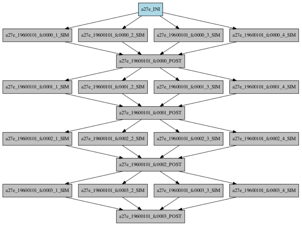
Our particular workflow consists of three different types of job. The first is the initialisation of the experiment and is only run once at the very beginning of the experiment. The second is the simulation, which is run once per individual in parallel in each generation. Finally, the postprocessing, which includes the crossover, is run once per generation. An example of a workflow for a toy experiment of four populations and four generations is shown in Fig. 2.
2.4.1 Initialisation
The initialisation script starts by setting up the directory in which the simulations are run by copying the executable of the model and the necessary input files into it. Included within the initialisation is a simulation run with a vector of the default parameters, and certain statistical measurements between its output and the observed data are taken that are necessary for postprocessing and calculation of the cost function. Finally, the script generates the initial set of vectors at random.
2.4.2 Simulation
The second script, which runs p times at each generation in parallel, starts by setting up the environment for each simulation. It then reads its corresponding vector from the generated set and edits the name lists to contain the updated parameters. Afterwards, the simulation is run and the cost function calculated.
2.4.3 Crossover
The final script runs once per generation after all simulations of the respective generation are completed. First, it reads the cost function statistics calculated after each simulation and uses them to calculate the ST score of SPOC and LPOC. It then ranks each of the simulations according to the sum of the two ST scores. Then it performs the crossover, as described in Sect. 2.3.1, to produce a new set of parameters in the same format so that it can be read by the following generation's simulation scripts.
2.5 Experiments
To investigate the potential of the BRKGA, different sets of experiments are run. Each set contains five experiments (to test consistency and robustness) with distinct and randomly generated initial populations, with 100 individual simulations over 100 iterations. Their details are summarised in Table 2.
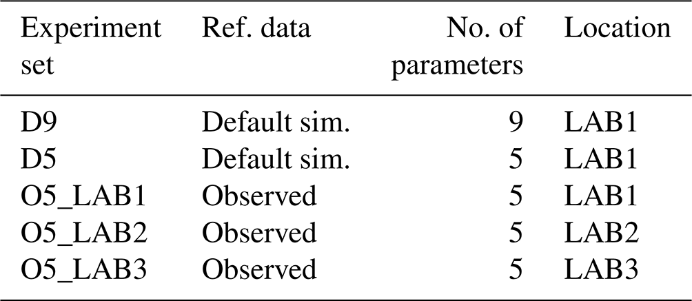
Initially, we determine the capabilities of the BRKGA by testing how well it can find a known set of parameters. To do this, experiment sets D9 and D5 are run using the output of a simulation with the default parameters being the reference data at location LAB1. In set D9, nine parameters are tested to check which ones can be constrained from SPOC and LPOC data. This leads us to select five parameters, which are tested in set D5 and, additionally, give us an indication of how the method behaves when different sizes of vectors of parameters are used.
Experiment set O5_LAB1 uses the BRKGA as intended, where the reference data are observed data from LAB1, and the outputs are analysed. This is further compared with experiment sets O5_LAB2 and O5_LAB3, which are run in LAB2 and LAB3, respectively. This is to investigate how the results obtained reflect the wider region.
Finally, cross-simulations are run, whereby a representative vector of parameters from each of the experiment sets O5_LAB1, O5_LAB2, and O5_LAB3 is selected to run a single simulation in the other two locations. This is to further check how robust the BRKGA is and if the vectors produced are representative of the region. In fact, a certain homogeneity is expected across the three locations because of their similar physical and biogeochemical properties. The BRKGA not capturing this homogeneity would suggest that the tool is compensating for other errors in the attempt to minimise the cost function resulting in an overfitting of the optimal vector of parameters.
3.1 Default data
3.1.1 The nine parameters (D9)
The evolution of the optimal sets of parameters in experiment set D9 is presented in Fig. 3. Figures 4 and 5 present the cost function of each optimal set per iteration and their corresponding statistics of the SPOC and LPOC. In all cases, most of the evolution occurs within the first 10 to 20 generations. This is evident from all figures, as the cost function decreases rapidly towards zero, and the optimal sets of parameters in all experiments initially fluctuate greatly before remaining at similar values for the remainder of the experiment. The spread of the values to which the parameters tend to converge varies strongly from one parameter to another. When a parameter evolves towards its corresponding default value in a consistent manner across the five replicate experiments, this suggests that it can be constrained from SPOC and LPOC variables with greater confidence and should be considered when trying to optimise the model against observed data. This is evident with wsbio and xremip, which return rapidly to the default value in most experiments. Other parameters, like wsbio2, wchld, wchldm, grazflux, and solgoc, show larger optimisation uncertainty but converge to within ±50 % of the default value in most experiments. On the other hand, if the optimal values for a parameter in each of the five experiments differ from each other and the default, then this suggests that they cannot be constrained from POC variables in the 0–1000 m domain. This can be seen with wsbio2max and caco3r. Differences between experiments are also indicative of tradeoffs between parameter changes and their impact on the cost function. For example, in experiment a274, its distinctly lower xremip value, along with its lower skill of LPOC (Fig. 5), suggests that it had optimised SPOC quickly at the expense of LPOC, causing the BRKGA to become trapped in a local minimum, as indicated by the higher overall cost.
The results of experiment D9, plus additional analyses that we report in Appendix A, provided the criteria to select the five parameters that were used in subsequent PO experiments. Quite obviously, the POC sinking speed, wsbio, and the specific remineralisation rate of both POC and GOC, xremip, were selected owing to their rapid and robust convergence to the expected values. In addition, wchld, wchldm, and grazflux, which showed vacillating convergence behaviour in D9, were selected owing to their important role in POC budgets. In particular, flux feeding (grazflux) can greatly attenuate the gravitational GOC flux in the upper mesopelagic while fragmenting a fraction of GOC to POC. The parameters wchld and wchldm control detrital POC formation through phytoplankton mortality and aggregation, especially during phytoplankton bloom collapse. Hence, their inclusion is further justified by the need to optimise parameters that control POC and GOC sources and not only sinks.
Figures A1 and A2 show the contribution of individual source and sink terms to the POC and GOC rates of change with the default vector of parameters, demonstrating the important role of the five selected parameters. Additional experiments (not shown) were run with solgoc and other parameters not included in Table 1, supporting the choice of the previous five parameters.
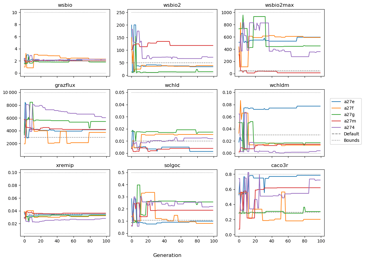

Figure 5Evolution of each optimal generation's bias, normalised standard deviation, correlation, and RMSE of experiment set D9.
3.1.2 The five parameters (D5)
The following plots analyse the results of experiment set D5. The evolution of the optimal vector of parameters from each generation is presented in Fig. 6. Figures 7 and 8 show the evolution of these experiments' statistics. When comparing these results to those of experiment set D9, an all-round improvement is visible. In all cases, the parameters are more consistent and are more likely to return to the default – and quicker. There is less indication of the experiments becoming stuck in a local minimum, while there exists a lower cost function elsewhere within the wider space. In all cases, the cost functions are lower, and the rest of the statistics are also better. Preliminary experiments where only wsbio, xremip, and grazflux were optimised (not shown) yielded even faster and more robust convergence to the expected parameter values. These results suggest that, with larger parameter sets, the BRKGA requires a larger population and a larger number of generations to be effective. However, given the difference in the results of sets D9 and D5, there is reason to believe that increasing the number of parameters in the BRKGA does not increase the dimensionality of the problem in the way that a brute-force approach would have. Finally, increasing the vector size, i.e. the number of parameters, increases the probability of the BRKGA becoming stuck in local minima while searching for the optimal set.
Experiment set D5 was additionally compared with a similarly structured experiment set that used a random search algorithm to verify the better efficacy of the BRKGA. The results of this comparison are in Appendix C.


Figure 8Evolution of each generation's optimal bias, normalised standard deviation, correlation, and RMSE in experiment set D5.
3.2 Observed data
3.2.1 Labrador Sea
Figure 9 shows the evolution of the optimal set of parameters in each generation of experiment set O5_LAB1. There are the following two types of behaviour observed: the parameters wchld and wchldm converge to a range that brackets the default values, whereas wsbio, grazflux, and xremip clearly deviate from the default values. Still, the latter three parameters behave consistently across the five replicate experiments, which is in line with how they behave in D5. The parameters grazflux and xremip move beyond the extreme bounds of the initial range. This is due to the slight perturbation of parameters after the crossover stage (Sect. 2.3.1). The results also illustrate the interdependence between the parameters, such that a decrease in wsbio leads to an increase in certain others (see Sect. 4). The rapid evolution at the beginning is evident in the large drop in the cost function that happens during the first 10 generations (Fig. 10). As expected, the cost function is higher overall than those of the experiments against the default outputs. From Fig. 11, we can see that most of the statistics improve very quickly at the start and that it is noticeable that the statistics for the LPOC are generally worse than the SPOC and hence make the larger contribution to the overall ST score. Figures 12 and 13 are Hovmöller plots of the POC concentration profiles over the annual cycle for experiment O5_LAB1 (observed, default model, and optimised model). Also included are the deviations in the default and optimised outputs with respect to the observed data. With the SPOC, the improvement is particularly noticeable in the reduction of the SPOC sinking plumes in the upper mesopelagic. Whereas mean biases are generally reduced, patches with positive/negative biases remain at different times and depths after optimisation, which is also reflected in the small improvements in correlation. It must be noted that the correlation coefficients for the simulations with default parameters were already high (0.96 for SPOC and 0.85 for LPOC) and thus difficult to improve. Further reduction in the LPOC misfit could have been impeded by the noisier nature of the observed LPOC data (Galí et al., 2022).
Figure 9Evolution of each generation's optimal set of parameters for experiment set O5_LAB1.
Figure 10Evolution of each generation's lowest ST score of experiment set O5_LAB1. The label of default refers to the cost function of the default simulation.
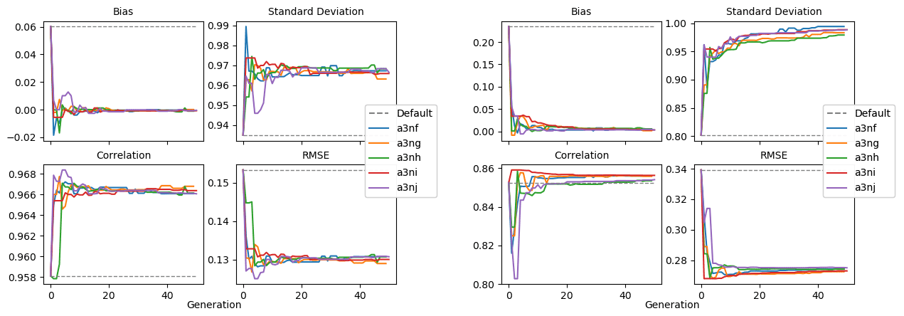
Figure 11Evolution of each generation's optimal bias, normalised standard deviation, correlation, and RMSE of experiment set O5_LAB1.
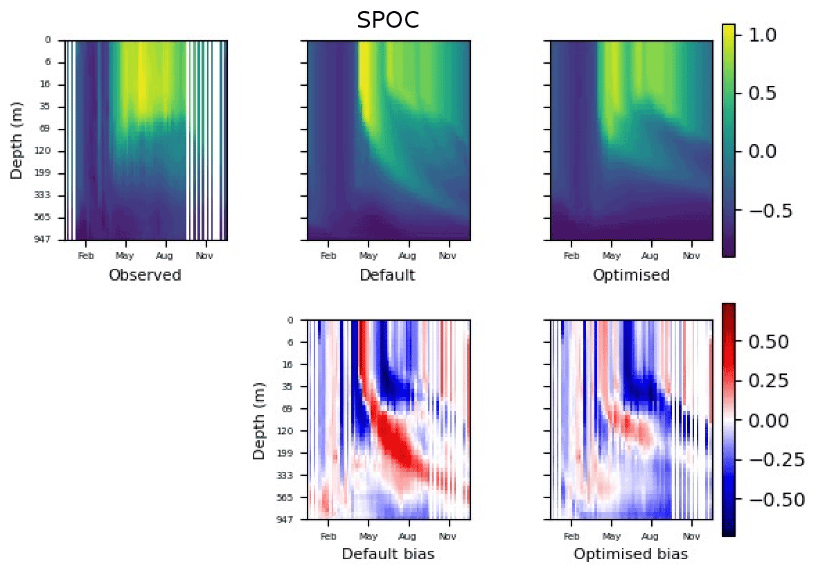
Figure 12The top row shows data plots of SPOC in log scale, for (left–right) observed data, the default parameter set's model output, and the optimised parameter set's model output. The bottom row shows the biases between the model outputs and observed data for the default parameter set (left) and optimised parameter set (right). Mean biases of the default and the optimised parameter sets are shown in Fig. 11.
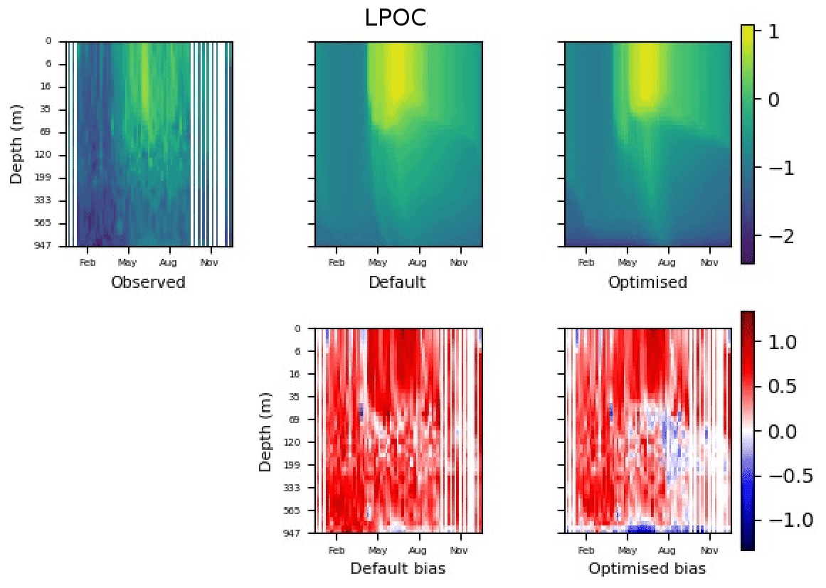
Figure 13The top row shows data plots of LPOC in log scale, for (left–right) observed data, the default parameter set's model output, and the optimised parameter set's model output. The bottom row shows the biases between the model outputs and observed data for the default parameter set (left) and optimised parameter set (right). Mean biases of the default and the optimised parameter sets are shown in Fig. 11.
3.2.2 Experiments in other locations and cross-testing
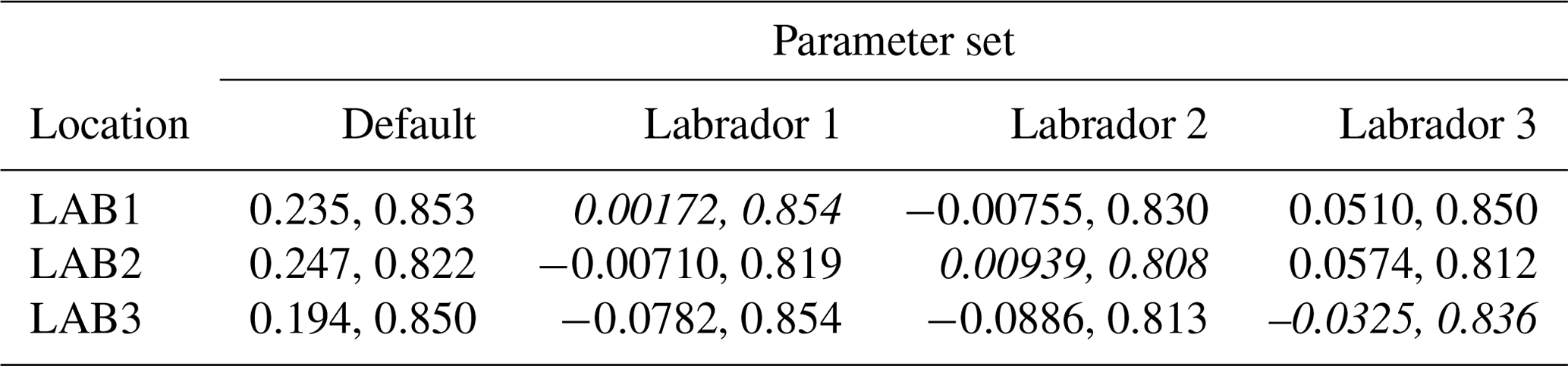
The experiments producing the median cost function for each set of O5_LAB1, O5_LAB2, and O5_LAB3 are presented in Table 3. We can see that the results are fairly consistent with each other, albeit some minor differences (for example wsbio in O5_LAB1 and grazflux in O5_LAB2), indicating that the genetic algorithm behaves consistently from a regional perspective. This consistency is further confirmed when cross-simulations are performed on the results. These cross-simulations are performed by using the parameter set produced for one location to run single simulations at the other two locations. The bias and correlation of SPOC and LPOC between the outputs of these simulations and the respective observed data are calculated. These statistics, along with the bias and correlation of the simulations with default parameters, are presented in Tables 4 (SPOC) and 5 (LPOC). In all cases, when a parameter set obtained from one location is applied to another, the outputs show reasonable consistency. For LPOC, all cross-tests show a substantial improvement in the bias with respect to the default outputs and very little improvement – if any – with correlation, which is consistent with the outputs from the original location. There are indications of consistency with SPOC, with nearly all showing an improvement with correlation, but it is less clear. This could be due to the default outputs' biases already being very low and their correlation being very high.
Table 3The final parameter sets of three genetic algorithm experiments run in three locations, along with the default.

Table 4Comparison of SPOC absolute bias and correlation of 12 single simulations run by crossing the four parameter sets (the default and three optimised sets produced by the BRKGA at three locations) with three locations. Values in italics mark the diagonals with equal locations and parameter sets.
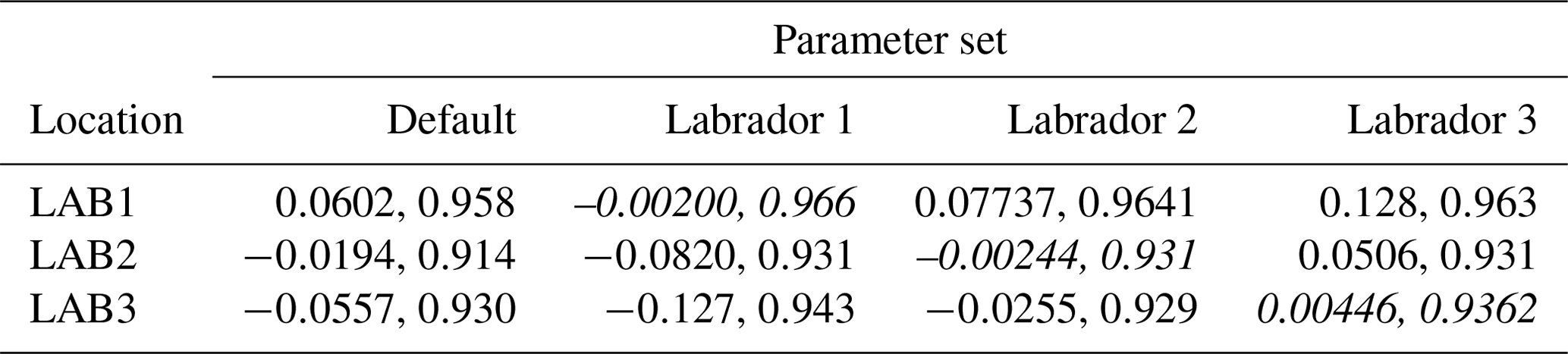
Table 5Comparison of LPOC absolute bias and correlation of 12 single simulations run by crossing the four parameter sets (the default and three optimised sets produced by the BRKGA at three locations) with three locations. Values in italics mark the diagonals with equal locations and parameter sets.
A set of experiments was designed to test the potential of a newly developed BRKGA. As a validation, the BRKGA was first tested against the output of a simulation produced with known default parameter settings. For the first set of experiments, we chose nine parameters, expressed as a vector, insuring a broad selection. This guided our choosing of parameters that could be constrained with confidence from the evaluated variables (in this case, SPOC and LPOC). In addition, in this set (and all others in the paper) five identical experiments were run at a time, and all results were similar to each other; this indicates that this method behaves consistently and reliably. The next set of experiments was identical to the previous set, except that there were only five parameters selected from the initial nine-parameter vector. This particular set of experiments produced results that were closer to the result of the default parameter vector with less computation. This leads us to believe that the size of the experiment required is dependent on the size of the parameter vector. One of the main contributions of this work is to use a state-of-the-art ocean model as a prior step to the calculation of the fitness function, with all the complexity that this option entails. This is only possible because of the aforementioned availability of computing power, and it is also highly facilitated by the usage of advanced scientific workflow solutions that allow the integration of the model executions in the evolutionary workflow (Oana and Spataru, 2016; Dueben and Bauer, 2018; Rueda-Bayona et al., 2020).
After the experiments against default data, the BRKGA was then tested by using observed data from ocean floats in the North Atlantic as the reference data. A set of five experiments was run for each BGC–Argo float annual time series, using the same settings as in the previous set. From Fig. 9, we can see that the results show a similar level of consistency to those with the default data. There is a visible improvement in the outputs of the simulations that use a set of parameters that have been optimised by the BRKGA compared to the outputs with the default parameter simulations (Figs. 12 and 13). However, most of the optimised parameter values tended rapidly towards the optimisation bounds (Table 1), and some even exceeded them thereafter because parameters were allowed to exceed the bounds by a small percentage in each generation. This behaviour makes us question whether the optimised values are realistic, although it is also possible that we imposed too-strict bounds in some cases, given the wide range of plausible ranges that characterises some parameters (see below). The problem of obtaining a right answer for the wrong reasons is common to all PO methods when applied to complex and heavily parameterised systems (Löptien and Dietze, 2019; Kriest et al., 2020). Therefore, PO must always be followed by a critical evaluation of the results. If a parameter converges repeatedly to unrealistic values, regardless of the value of other parameters, this may indicate that a process is poorly represented by the model equations. In such cases, PO can prompt further model development.
Another concern that arises from the results is the need to carefully evaluate the behaviour of the cost function. This is well illustrated by Figs. 4 and 5, which show that, on occasion, some statistics were improved at the expense of others, for example, bias at the expense of correlation. Correctly balancing bias, variability, and pattern (correlation) statistics in the cost function is critical to obtain meaningful PO results. Traditional cost functions based solely on the RMSE tend to reward solutions with too-low variability, whereby the positive biases cancel out the negatives (Jolliff et al., 2009, and references therein). Cost functions such as the ST score used here (Jolliff et al., 2009) were designed to avoid this problem. However, their behaviour is also sensitive to the overall variability and the signal-to-noise ratio in the data. Our preliminary tests suggested slightly better BRKGA performance after the logtransformation of the data. This procedure reduced the weight of the very high POC concentrations present only in the surface layer in spring–summer, favouring the representation of the portions of the water column with lower POC (i.e. the mesopelagic). Unlike the model outputs used to test the BRKGA in the first set of experiments, the BGC–Argo POC estimates are noisy. Therefore, the cost function may have been less effective when faced with the observed data. The performance of the cost function could also be improved by applying different weights to each variable, in this case SPOC and LPOC, which is common practice when the reference variables exhibit very different variability ranges (Friedrichs et al., 2007; Ayata et al., 2013).
Further work quantifying the effectiveness of the cost functions across different situations would probably improve the efficacy of the BRKGA. Yet, it must be highlighted that the test case chosen to evaluate the BRKGA is an exigent one because model skill was already very good with the default parameters, even though PISCES was not originally tuned to fit these particular observations. Ongoing work with a different optimisation case indicates that the BRKGA can produce larger and simultaneous improvements in all skill metrics when starting from a state of very poor model performance, which is, in this case, the seasonal cycle of sea surface chlorophyll a in the Tasman Sea ( Joan Llort,, personal communication, 2022; data not shown). Therefore, the tradeoffs between skill metrics observed here during the evolution of the experiments may indicate that the optimisation was operating close to the best skill attainable with a given set of model equations and considering observational uncertainty.
As a further test of our approach, two more sets of experiments were carried out in different locations in the Labrador Sea, resulting in a reasonable consistency of the optimal parameter set across the region. To confirm this, the optimal parameter sets for the three locations were cross-referenced by using each parameter set in each of the other two locations in single simulations. Results from this cross-testing suggest that the parameters produced have the potential to be representative of the region or even exchangeable among multiple locations (Table 3), meaning that the BRKGA is not compensating for other biases (e.g. physics) by overfitting (Löptien and Dietze, 2019; Kriest et al., 2020). This is an important aspect because it means the BRKGA could be used to investigate the large-scale spatial variability in key biogeochemical parameters. In particular, in the past decade, several authors have investigated the spatial variability in the transfer efficiency of POC from the surface ocean to its interior using different approaches and arriving at contrasting conclusions (Henson et al., 2011; Marsay et al., 2015; Guidi et al., 2015; Weber et al., 2016; Schlitzer, 2004; Wilson et al., 2015). Such spatial variability would be very difficult to establish in a three-dimensional framework because of the high computational cost required. This is an example of the still-open scientific questions that could be tackled with our approach.
The optimisation of PISCES parameters against BGC–Argo presented in our study illustrates how PO can help us understand a dynamical system better. Here we will briefly discuss the lessons learnt from the O5 experiments, while keeping in mind that a detailed review of PISCES parameter values and their biogeochemical implications is beyond the scope of this paper. It is also noteworthy that the interpretation provided here draws only from the analysis of the best-performing parameter set in each BRKGA experiment. Full exploitation of the results, with thousands of alternative model realisations, could yield further insights on how parameters interact in a space constrained by optimal model performance.
In the three O5 experiments, wsbio converged to values between 0 and 1 m d−1. The decrease in the POC sinking speed improved the fit to observations by reducing the plumes of sinking POC that formed below intense phytoplankton blooms in the simulations (Fig. 12). Galí et al. (2022) identified these plumes as being the main reason for SPOC model–data misfit in the upper mesopelagic in several subpolar locations in the Northern and Southern hemispheres. The decrease in wsbio effectively turned the SPOC fraction into suspended POC, which is plausible according to field studies that sorted POC fractions according to their sinking speed (Riley et al., 2012; Baker et al., 2017). The evolution of the remaining parameters acted to adjust the magnitude and shape of POC vertical profiles. Increased xremip implies a steeper vertical decrease in both POC and GOC, with a stronger effect on POC given its much longer residence time in the mesopelagic. The xremip parameter represents the maximal specific remineralisation rate attainable in the model, corresponding to freshly produced detritus, normalised to a temperature of 0 ∘C with a power law temperature dependence (Aumont et al., 2015). Our optimised xremip range, 0.078–0.114 d−1, is consistent with the median of the highest values found across six field and laboratory studies when normalised to 0∘ in the same way, i.e. 0.10 d−1 (Belcher et al., 2016, and references therein), with an absolute maximum of 0.135 d−1 (Iversen and Ploug, 2010). Decreased POC sinking speed and increased remineralisation would deplete mesopelagic POC during the productive season (central panel of Fig. B1) and, hence, SPOC if they were not compensated by other processes. In our PO experiments, this deficit was compensated by slightly increased surface microphytoplankton mortality and aggregation (wchld and wchldm), which supply SPOC and LPOC.
Interpretation of the evolution of the grazflux parameter is more complex. The flux-feeding rate depends on the product of mesozooplankton biomass, grazflux, and particle sinking speed. In PISCES, a fraction of the intercepted GOC is fragmented into POC. Therefore, flux feeding acts to remove POC and GOC (preferentially the fast-sinking GOC) and simultaneously produce POC; this process is becoming an important POC source in the lower mesopelagic (Figs. A1 and A2). Although a decrease in grazflux provided the best fit to observations, an increase in grazflux could also improve model skill, as shown by the relatively good skill of experiment a3nj during the first few generations (Figs. 9 and 10). This dual behaviour is confirmed by sensitivity analyses (Fig. B3) which show that, for a given xremip, a decrease in POC (which improves the model–data fit in the upper mesopelagic) can be achieved by either increasing or decreasing grazflux. Overall, these findings provide further evidence for the difficulty of constraining this important parameter (Jackson, 1993; Stemmann et al., 2004; Gehlen et al., 2006; Stukel et al., 2019).
The selection of a subset of model parameters is a common limitation of PO experiments, and although we based it on objective criteria, we acknowledge that it remains somewhat arbitrary. The stepwise reduction in the number of parameters from nine to five obeys the need to assess the GA performance with a varying number of parameters and also to reduce the degrees of freedom, given that only two variables were used as reference observations. Among the excluded parameters, wsbio2 certainly deserves examination in future experiments, given its primary control on the fate of GOC (large detritus). There are the following three main reasons that led us to exclude wsbio2 from this work: (1) our optimisation exercise focused on POC stocks, which are largely dominated by the SPOC fraction that typically represents around 85 % of total POC (Galí et al., 2022, and references therein), (2) experiment set D9 suggested that, unlike wsbio, wsbio2 might be difficult to constrain even from error-free data provided by the default model run, and (3) estimation of wsbio2 relies, more than any other parameter, on observational LPOC estimates which suffer from larger uncertainty than SPOC estimates (Galí et al., 2022).
Mesopelagic POC dynamics provide a relevant optimisation case because of their role in oceanic carbon sequestration (Martin et al., 2020; Henson et al., 2022). Beyond the specific results presented here, our approach has the additional value of showing that similarly good fits can be obtained with different combinations of parameter values (Ward et al., 2010), pointing to the many degrees of freedom in PISCES and similar OBGCMs. Hence, we call for a continuous reassessment of parametric uncertainty as new types of observations (e.g. from BGC–Argo) become available. Future work is granted to study the sensitivities, interdependencies, and optimal values of PISCES parameters through more comprehensive experiments.
The GA developed shows potential in effectively constraining the parameters of the NEMO–PISCES ocean biogeochemistry model in a way that can be extended to similar models. Our GA is embedded in the workflow manager Autosubmit, which seamlessly handles thousands of individual simulations alongside the GA calculations. This key feature makes the process of objective parameter optimisation automatic, reproducible, and portable across different high-performance computing platforms.
We proposed an experimental protocol that consists of two main phases. First, the optimisation runs against the output of the default model, whose parameter values are known beforehand, to identify the parameters that can be effectively constrained when the evaluation data can be perfectly matched by the model. Second, the subset of selected parameters is optimised against the actual observations. This protocol increases the efficiency and robustness of the optimisation by reducing the parameter space. Based on the experience acquired through the development of this tool, we make the following three main recommendations that can maximise the efficacy of the GA for a given research problem:
-
It may be necessary to adjust the GA metaparameters to optimise the balance between convergence speed and parameter space exploration.
-
The cost function has to be selected, keeping in mind the tradeoffs between bias, dispersion, and pattern (correlation) statistics, and a single formula is unlikely to serve all purposes equally well.
-
Realistic parameter bounds are key to ensure that the results produced are sensible from a scientific point of view, and the optimisation results have to be critically evaluated a posteriori.
The use of POC estimates from BGC–Argo floats for the optimisation of biogeochemical parameters is a novel approach, as previous studies generally used target variables such as chlorophyll a, nutrients, or oxygen or sparse process rate measurements (primary production and vertical particle fluxes). The joint use of ocean observations from autonomous instruments and objective optimisation techniques is a powerful tool to improve the predictive skill of Earth system models.
This Appendix shows the rates of detrital POC production (sources) and consumption (sinks), as represented in PISCES equations, with default parameters, over the annual cycle in the Labrador Sea between the surface and 1000 m depth. The magnitude of the POC and GOC cycling rates associated to each process, and their distribution in the water column, were used to select the parameters for optimisation experiments (focusing on the mesopelagic layer).
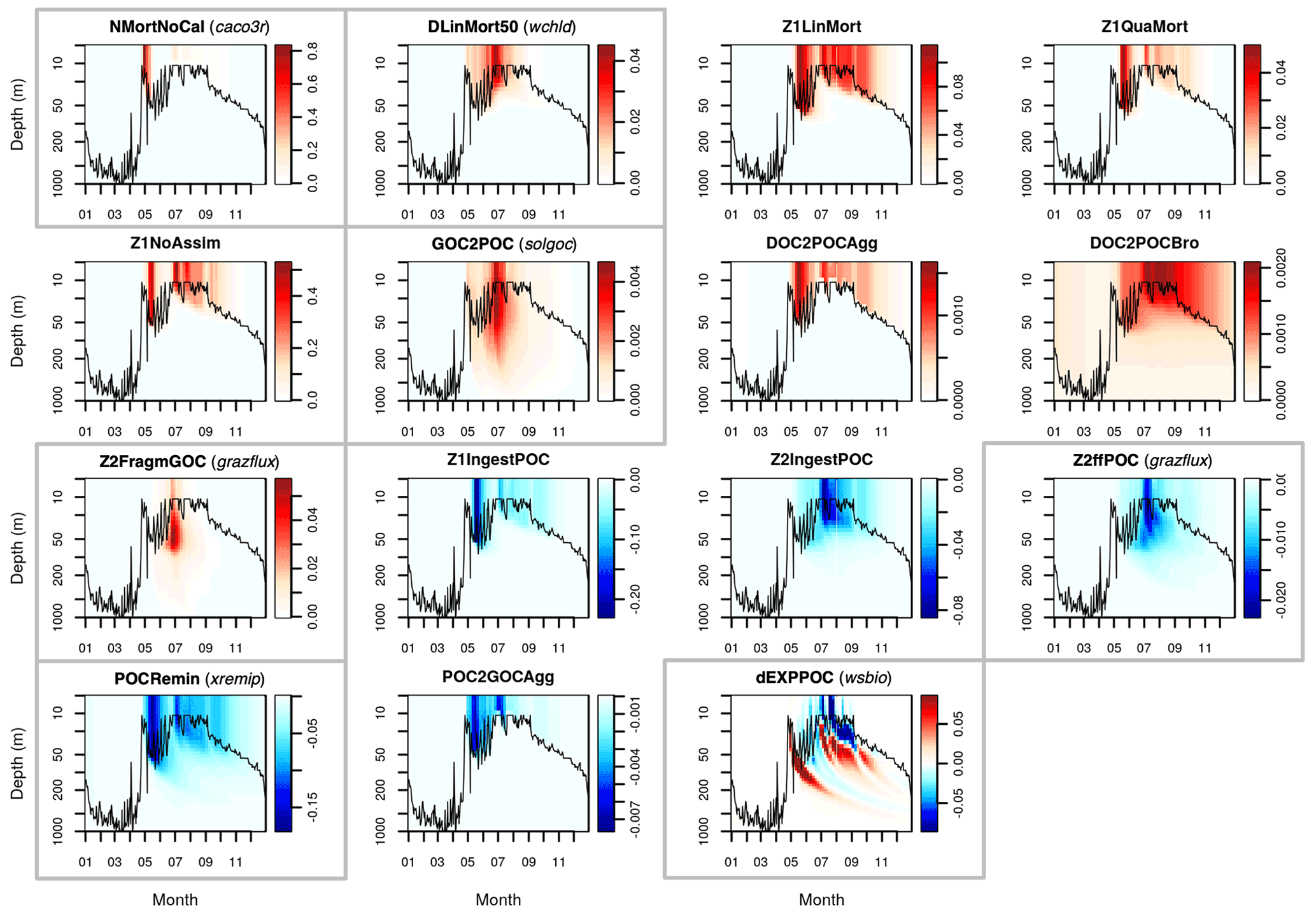
Figure A1Sources (red) and sinks (blue) of the PISCES tracer POC (small detrital particulate organic carbon) over the annual cycle in the Labrador Sea with default model parameters. Rates are in millimoles of carbon per metre cubed per day (mmol C m−3 d−1). Panels showing process rates that are controlled by parameters optimised in this study are boxed. From left to right and from to top bottom, we show the non-calcifying nanophytoplankton mortality (NMortNoCAL; partly controlled by caco3r), 50 % of diatoms linear mortality (DLinMort50; controlled by wchld), microzooplankton linear mortality (Z1LinMort), microzooplankton quadratic mortality (Z1QuaMort), unassimilated fraction of total microzooplankton ingestion (Z1NoAssim), GOC-to-POC breakdown upon bacterial solubilisation (GOC2POC; controlled by solgoc), dissolved organic carbon (DOC)-to-POC aggregation caused by turbulence (DOC2POCAgg) and Brownian motion (DOC2POCBro), GOC fragmentation upon mesozooplankton flux feeding (Z2FragmGOC; controlled by grazflux), microzooplankton POC ingestion (Z1IngestPOC), mesozooplankton POC ingestion (Z2IngestPOC), mesozooplankton flux feeding on sinking POC (Z2ffPOC; controlled by grazflux), POC degradation (POCRemin; controlled by xremip); POC-to-GOC aggregation caused by turbulence and differential settling (POC2GOCAgg), and gravitational POC sinking expressed as net volumetric rates of change (dEXPPOC; controlled by wsbio). Details on the POC parameterisation in PISCES can be found in Aumont et al. (2015, 2017).

Figure A2Sources (red) and sinks (blue) of the PISCES tracer GOC (large detrital particulate organic carbon) over the annual cycle in the Labrador Sea with default model parameters. Rates are in millimoles of carbon per metre cubed per day (mmol C m−3 d−1). Panels showing process rates that are controlled by parameters optimised in this study are boxed. From left to right and from to top bottom, we show the calcifying nanophytoplankton mortality (NMortCAL; partly controlled by caco3r), 50 % diatoms linear mortality (DLinMort50; controlled by wchld), diatoms quadratic mortality (DQuaMort; controlled by wchldm), mesozooplankton mortality (Z2LinMort), fecal pellet production upon predation on mesozooplankton by upper trophic levels (Z2QuaMortPe), unassimilated fraction of total mesozooplankton ingestion (Z2NoAssim), DOC-to-GOC aggregation caused by turbulence and Brownian motion (DOC2GOCAgg), POC-to-GOC aggregation caused by turbulence and differential settling (POC2GOCAgg), mesozooplankton flux feeding on sinking GOC (Z2ffGOC; controlled by grazflux), GOC fragmentation upon mesozooplankton flux feeding (Z2FragmGOC; controlled by grazflux), GOC degradation (GOCRemin; controlled by xremip), GOC-to-POC breakdown upon bacterial solubilisation (GOC2POC; controlled by solgoc), and gravitational GOC sinking expressed as net volumetric rates of change (dEXPGOC; controlled by wsbio2 and wsbio2max). Details on the GOC parameterisation in PISCES can be found in Aumont et al. (2015).
This Appendix shows the sensitivity of the POC tracer concentration to variations in the PISCES parameters xremip, wsbio, and grazflux in pairwise combinations. A total of 10 different values distributed over the range specified in Table 1 are used for each parameter. Mean POC concentrations for each pairwise combination of parameters are computed over the following three distinct depth intervals: 0–100 m (epipelagic), 100–500 m (upper mesopelagic), and 500–1000 m (lower mesopelagic) and for three periods of 4 months each. These sensitivity tests illustrate the difficulty of understanding and optimising parameter interactions in models such as PISCES, even with a small subset of parameters, which justifies the need for optimisation approaches such as the BRKGA presented here.
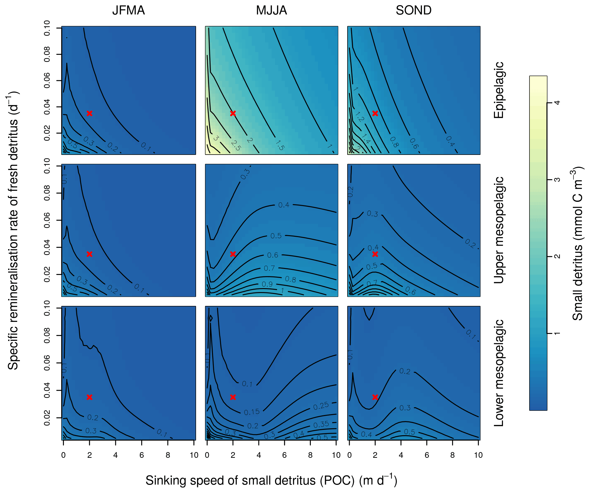
Figure B1Combined sensitivity of the PISCES POC tracer to the specific degradation rate of detrital organic carbon particles (xremip; x axis) and the sinking speed (wsbio; y axis). The panels show mean POC concentrations for different 4-month periods over the annual cycle (columns) and layers (rows). Epipelagic is 0–100 m, upper mesopelagic is 100–500 m, and lower mesopelagic is 500–1000 m. Red crosses show the default PISCES parameter values.

Figure B2Combined sensitivity of the PISCES POC tracer to the mesozooplankton flux-feeding cross section (grazflux; x axis) and the sinking speed (wsbio; y axis). The panels show mean POC concentrations for different 4-month periods over the annual cycle (columns) and layers (rows). Epipelagic is 0–100 m, upper mesopelagic is 100–500 m, and lower mesopelagic is 500–1000 m. Red crosses show the default PISCES parameter values.
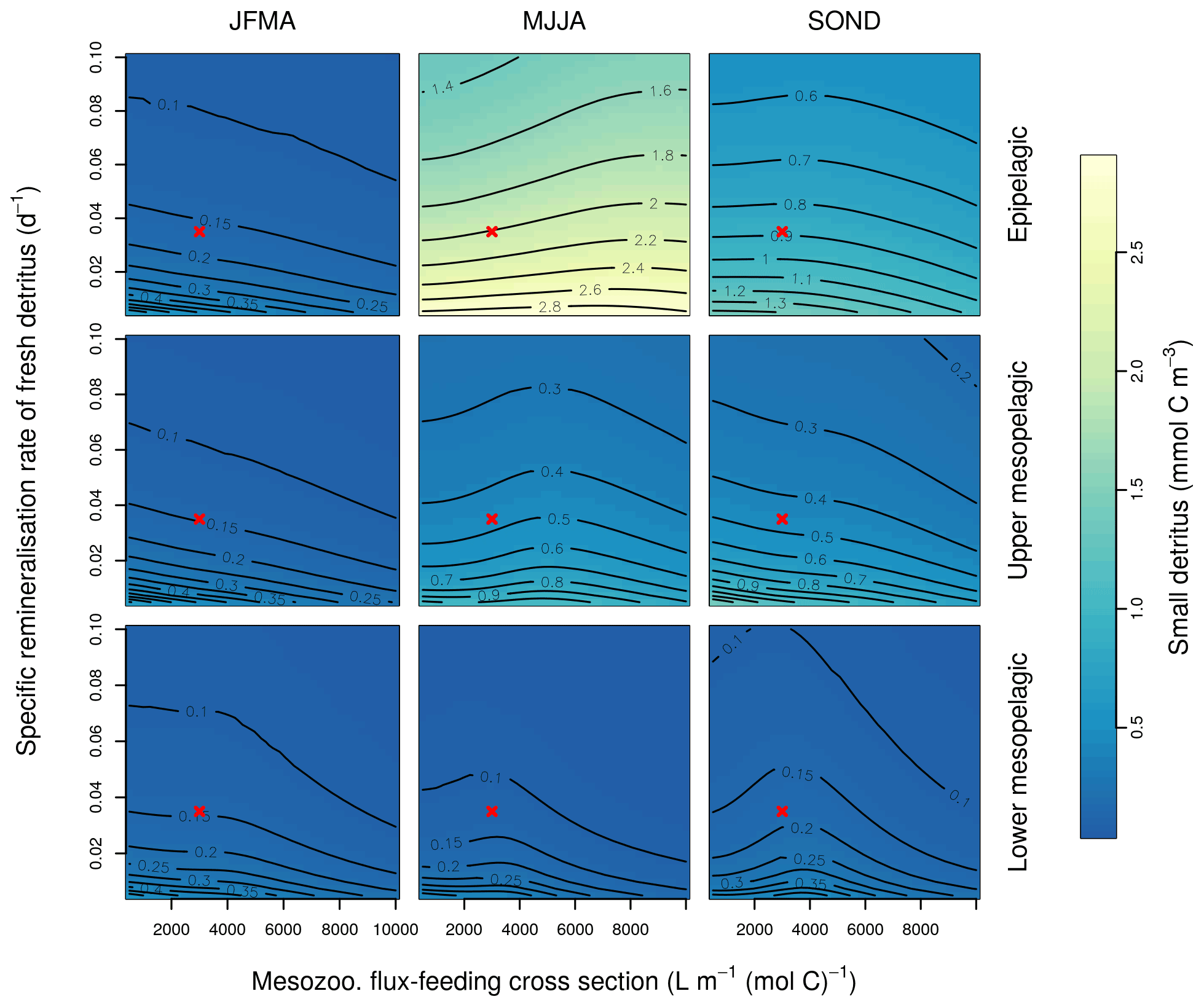
Figure B3Combined sensitivity of the PISCES POC tracer to the specific degradation rate of detrital organic carbon particles (xremip; x axis) and the mesozooplankton flux-feeding cross section (grazflux, y axis). The panels show mean POC concentrations for different 4-month periods over when you compare the annual cycle (columns) and layers (rows). Epipelagic is 0–100 m, upper mesopelagic is 100–500 m, and lower mesopelagic is 500–1000 m. Red crosses show the default PISCES parameter values.
To evaluate the effectiveness of the BRKGA, we compared the results of experiment set D5 to that of a random search algorithm, D5_rand, which is identical to D5, except that every parameter set in every generation is generated at random, with the exception of the most elite one from the previous generation. To compare the two sets of experiments, the experiment with the median cost function is considered in both cases, and the absolute difference between the final parameters and the default ones are calculated (Table C1). The statistics of these two median experiments are presented in Fig. C1, alongside with the standard deviation of each statistic. The latter provides a metric for comparing the convergence robustness between (D5 and D5_rand). Looking at both plots and the tables that compare sets D5 and D5_rand, we can see that the GA outperforms the random search (RS) in almost every sense, with few exceptions. The final parameter sets of the GA are more consistent than the RS, and all of the individual GA experiments outperform the RS ones in the cost function and all of the statistics. The standard deviation of the statistics is higher for the random search, providing further evidence that the convergence behaviour of the GA is more robust.
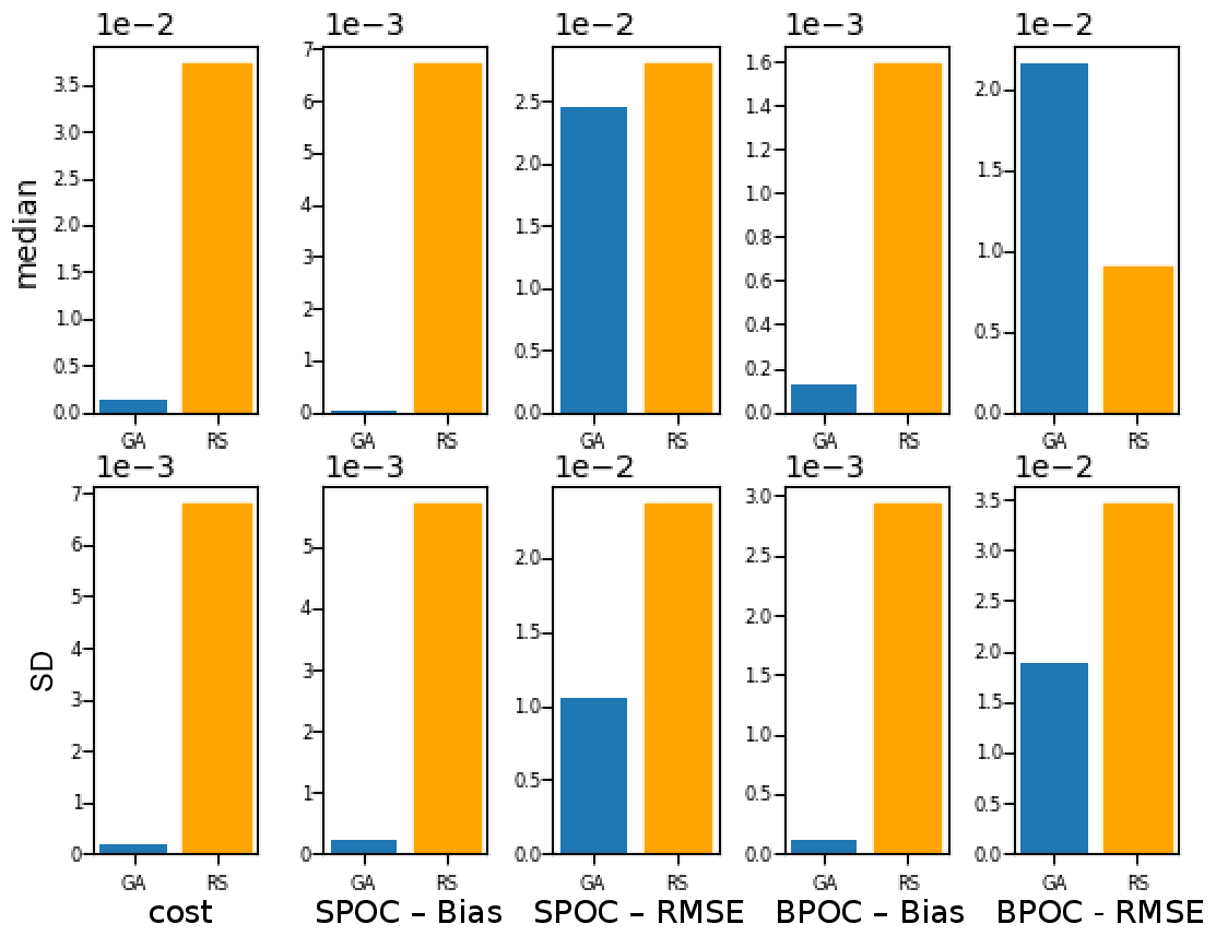
Figure C1Comparison of the meta-analyses of experiment sets D5 and D5_rand. The top row, the median, compares the statistics of the experiments with the median cost function in each case. The bottom row, the SD, is the standard deviation of all experiments of each statistic in each case.
Table C1Absolute differences between the final parameter set of the median experiments of sets D5 and D5_rand and the default parameter set.

The code of NEMO v4.0.1 and PISCES-v2_RC are publicly available at https://www.nemo-ocean.eu/ (last access: April 2021), https://doi.org/10.5281/zenodo.3878122 (Madec et al., 2022). The PISCES 1D configuration used in this study is available at https://earth.bsc.es/gitlab/mgalitap/p1d_share/-/tree/gapoc/ (last access: May 2021) and https://doi.org/10.5281/zenodo.5243343 (Galí et al., 2021b). The code for the workflow of the genetic algorithm is readily available at https://doi.org/10.5281/zenodo.5205760 (Falls et al., 2021).
These data were collected and made freely available by the international Argo programme and the national programmes that contributes to it (https://argo.ucsd.edu, last access: April 2021; https://www.ocean-ops.org, last access: May 2021). The Argo programme is part of the Global Ocean Observing System. The repository that contains the processed BGC–Argo data and matching PISCES 1D simulations, titled “Datasets for the comparison between POC estimated from BGC–Argo floats and PISCES model simulations”, is readily available at https://doi.org/10.5281/zenodo.5139602 (Galí et al., 20211).
MF wrote the paper, with contributions from all co-authors. MC and MA contributed to the topics of computing and GAs. MG, RB, and JL contributed to the topics of ocean biogeochemistry. MF developed the code of the workflow of the GA (including the implementation of the GA itself and the configuration of the workflow manager) and developed the code to produce the figures and the data in the tables. MC developed the configuration of NEMO-PISCES for the MareNostrum 4 HPC platform and provided guidance to maximise the workflow efficiency. MG configured the PISCES 1D offline simulations and processed the observed data from the BGC–Argo floats. MG and RB conceived the study.
The contact author has declared that none of the authors has any competing interests.
Publisher's note: Copernicus Publications remains neutral with regard to jurisdictional claims in published maps and institutional affiliations.
The simulations analysed in the paper were performed using the internal computing resources available at the Barcelona Supercomputing Center. The authors acknowledge the support of Pierre-Antoine Bretonnière and Margarida Samsó, for downloading and storing the Argo data, Daniel Beltran and Wilmer Uruchi, for their technical support with Autosubmit, Hervé Claustre, for guidance on BGC–Argo data processing, Olivier Aumont, for guidance on PISCES-v2_RC structure and parameters, Xavier Yepes, for guidance on the BRKGA, and Thomas Arsouze, for technical support with the PISCES 1D configuration. Martí Galí has received financial support through the Postdoctoral Junior Leader Fellowship Programme from the La Caixa Banking Foundation (ORCAS project; grant no. LCF/BQ/PI18/11630009) and through the OPERA project funded by the Ministerio de Ciencia, Innovación y Universidades (grant no. PID2019-107952GA-I00). Raffaele Bernardello acknowledges support from the Ministerio de Ciencia, Innovación y Universidades, as part of the DeCUSO project (grant no. CGL2017-84493-R). The authors thank Urmas Raudsepp and one anonymous referee, for their constructive comments that improved the original work.
This research has been supported by the Fundación Bancaria Caixa d'Estalvis i Pensions de Barcelona (grant no. LCF/BQ/PI18/11630009) and the Ministerio de Ciencia e Innovación (grant nos. PID2019-107952GA-I00 and CGL2017-84493-R).
This paper was edited by Olivier Marti and reviewed by Urmas Raudsepp and one anonymous referee.
Anav, A., Friedlingstein, P., Kidston, M., Bopp, L., Ciais, P., Cox, P., Jones, C., Jung, M., Myneni, R., and Zhu, R.: Evaluating the Land and Ocean Components of the Global Carbon Cycle in the CMIP5 Earth System Models, J. Climate, 26, 6801–6843, https://doi.org/10.1175/JCLI-D-12-00417.1, 2013. a
Aumont, O., Ethé, C., Tagliabue, A., Bopp, L., and Gehlen, M.: PISCES-v2: an ocean biogeochemical model for carbon and ecosystem studies, Geosci. Model Dev., 8, 2465–2513, https://doi.org/10.5194/gmd-8-2465-2015, 2015. a, b, c, d, e, f, g
Aumont, O., van Hulten, M., Roy-Barman, M., Dutay, J.-C., Éthé, C., and Gehlen, M.: Variable reactivity of particulate organic matter in a global ocean biogeochemical model, Biogeosciences, 14, 2321–2341, https://doi.org/10.5194/bg-14-2321-2017, 2017. a, b, c, d
Ayata, S. D., Lévy, M., Aumont, O., Sciandra, A., Sainte-Marie, J., Tagliabue, A., and Bernard, O.: Phytoplankton growth formulation in marine ecosystem models: Should we take into account photo-acclimation and variable stoichiometry in oligotrophic areas?, J. Marine Syst., 125, 29–40, https://doi.org/10.1016/j.jmarsys.2012.12.010, 2013. a, b, c
Bagniewski, W., Fennel, K., Perry, M. J., and D'Asaro, E. A.: Optimizing models of the North Atlantic spring bloom using physical, chemical and bio-optical observations from a Lagrangian float, Biogeosciences, 8, 1291–1307, https://doi.org/10.5194/bg-8-1291-2011, 2011. a
Belcher, A., Iversen, M., Giering, S., Riou, V., Henson, S. A., Berline, L., Guilloux, L., and Sanders, R.: Depth-resolved particle-associated microbial respiration in the northeast Atlantic, Biogeosciences, 13, 4927–4943, https://doi.org/10.5194/bg-13-4927-2016, 2016. a
Boyd, P. W., Claustre, H., Levy, M., Siegel, D. A., and Weber, T.: Multi-faceted particle pumps drive carbon sequestration in the ocean, Nature, 568, 327–335, https://doi.org/10.1038/s41586-019-1098-2, 2019. a
Briggs, N., Dall'Olmo, G., and Claustre, H.: Major role of particle fragmentation in regulating biological sequestration of CO2 by the oceans, Science, 367, 791–793, https://doi.org/10.1126/science.aay1790, 2020. a
Broekema, C.P. Van Nieuwpoort, R. V. and Bal, H. E.: ExaScale high performance computing in the square kilometer array, Astro-HPC, 12, 9–16, https://doi.org/10.1145/2286976.2286982, 2012. a
Burd, A., Hansell, D., Steinberg, D., Anderson, T., Arístegui, J., Baltar, F., Beaupré, S. R., Buesseler, K., DeHairs, F., Jackson, G., Kadko, D., Koppelmann, R., Lampitt, R., Nagata, T., Reinthaler, T., Robinson, C., Robison, B. H., Tamburini, C., and Tanaka, T.: Assessing the apparent imbalance between geochemical and biochemical indicators of meso- and bathypelagic biological activity: What the is wrong with present calculations of carbon budgets?, Deep-Sea Res. Pt. II, 57, 1557–1571, https://doi.org/10.1016/j.dsr2.2010.02.022, 2010. a
Casanova, H., Legrand, A., and Robert, Y.: Parallel Algortihms, Chapman and hall/CBC Press, https://doi.org/10.1201/9781584889465, 2011. a
Claustre, H., Johnson, K., and Takeshita, Y.: Observing the Global Ocean with Biogeochemical-Argo, Annu. Rev. Mar. Sci., 12, 23–48, https://doi.org/10.1146/annurev-marine-010419-010956, 2020. a
De Jong, K. A., Spears, W. M., and Gordon, D. F.: Using genetic algorithms for concept learning, Mach. Learn., 13, 161–188, https://doi.org/10.1007/BF00993042, 1993. a
Dueben, P. D. and Bauer, P.: Challenges and design choices for global weather and climate models based on machine learning, Geosci. Model Dev., 11, 3999–4009, https://doi.org/10.5194/gmd-11-3999-2018, 2018. a
Eyring, V., Bony, S., Meehl, G. A., Senior, C. A., Stevens, B., Stouffer, R. J., and Taylor, K. E.: Overview of the Coupled Model Intercomparison Project Phase 6 (CMIP6) experimental design and organization, Geosci. Model Dev., 9, 1937–1958, https://doi.org/10.5194/gmd-9-1937-2016, 2016. a
Falls, M., Galí, M.m and Castrillo, M.: Genetic Algorithm Pisces 1D Workflow and config files, Zenodo [code], https://doi.org/10.5281/zenodo.5205760, 2021. a
Fasham, M. J. R., Ducklow, H. W., and McKelvie, S. M.: A nitrogen-based model of plankton dynamics in the oceanic mixed layer, J. Mar. Res., 48, 591–639, https://doi.org/10.1357/002224090784984678, 1990. a, b
Fennel, K., Losch, M., Schroter, J., and Wenzel, M.: Testing a marine ecosystem model: sensitivity analysis and parameter optimization, J. Marine Syst., 28, 45–63, https://doi.org/10.1016/S0924-7963(00)00083-X, 2000. a
Flato, G.: Earth system models: an overview, WIREs Clim. Change, 2, 783–800, https://doi.org/10.1002/wcc.148, 2011. a
Friedrichs, M. A., Dusenberry, J. A., Anderson, L. A., Armstrong, R. A., Chai, F., Christian, J. R., Doney, S. C., Dunne, J., Fujii, M., Hood, R., McGillicuddy Jr., D. J., Moore, J. K., Schartau, M., Spitz, Y. H., and Wiggert, J. D.: Assessment of skill and portability in regional marine biogeochemical models: Role of multiple planktonic groups, J. Geophys. Res., 112, 1937–1958, https://doi.org/10.1029/2006JC003852, 2007. a, b, c
Galbraith, E. D., Dunne, J. P., Gnanadesikan, A., Slater, R. D., Sarmiento, J. L., Dufour, C. O., de Souza, G. F., Bianchi, D., Claret, M., Rodgers, K. B., and Marvasti, S. S.: Complex functionality with minimal computation: Promise and pitfalls of reduced‐tracer ocean biogeochemistry models, J. Adv. Model. Earth Sy., 7, 2012–2018, https://doi.org/10.1002/2015MS000463, 2015. a
Galí, M., Benardello, R., Falls, M., Claustre, H., and Aumont, O.: Datasets for the comparison between POC estimated from BGC-Argo floats and PISCES model simulations (1.0.0), Zenodo [data set], https://doi.org/10.5281/zenodo.5139602, 2021a. a
Galí, M., Benardello, R., Falls, M., Claustre, H., and Aumont, O.: PISCES-v2 1D configuration used to study POC dynamics as observed by BGC-Argo floats, Zenodo [code], https://doi.org/10.5281/zenodo.5243343, 2021b. a
Galí, M., Falls, M., Claustre, H., Aumont, O., and Bernardello, R.: Bridging the gaps between particulate backscattering measurements and modeled particulate organic carbon in the ocean, Biogeosciences, 19, 1245–1275, https://doi.org/10.5194/bg-19-1245-2022, 2022. a, b, c, d, e, f, g, h
Gaudier, F.: URANIE: The CEA/DEN Uncertainty and Sensitivity platform, Sixth International Conference on Sensitivity Analysis of Model Output, 2, 7660–7661, https://doi.org/10.1016/j.sbspro.2010.05.166, 2010. a
Gehlen, M., Bopp, L., Emprin, N., Aumont, O., Heinze, C., and Ragueneau, O.: Reconciling surface ocean productivity, export fluxes and sediment composition in a global biogeochemical ocean model, Biogeosciences, 3, 521–537, https://doi.org/10.5194/bg-3-521-2006, 2006. a
Goncalves, J. and Resende, M.: Biased random-key genetic algorithms for combinatorial optimization, J. Heuristics, 17, 487–525, https://doi.org/10.1007/s10732-010-9143-1, 2011. a, b
Gruber, N., Clement, D., Carter, B. R., Feely, R. A., Heuven, S., Hoppema, M., Ishii, M., Key, R. M., Kozyr, A., Lauvset, S. K., Lo Monaco, C., Mathis, J. T., Murata, A., Olsen, A., Perez, F. F., Sabine, C. L., Tanhua, T., and Wanninkhof, R.: The oceanic sink for anthropogenic CO2 from 1994 to 2007, Science, 363, 1193–1199, https://doi.org/10.1126/science.aau5153, 2019. a
Guidi, L., Legendre, L., Reygondeau, G., Uitz, J., Stemmann, L., and Henson, S. A.: A new look at ocean carbon remineralization for estimating deepwater sequestration, Global Biogeochem. Cy., 29, 1044–1059, https://doi.org/10.1002/2014GB005063, 2015. a
Henson, S. A., Sanders, R., Madsen, E., J., M. P., Le Moigne, F., and Quartly, G. D.: A reduced estimate of the strength of the ocean's biological carbon pump, Geophys. Res. Lett., 38, L04606, https://doi.org/10.1029/2011GL046735, 2011. a
Henson, S. A., Laufkötter, C., Leung, S., Giering, S. L. C., Palevsky, H., and Cavan, E. L.: Uncertain response of ocean biological carbon export in a changing world, Nat. Geosci., 15, 248–254, https://doi.org/10.1038/s41561-022-00927-0, 2022. a, b, c
Iversen, M. H. and Ploug, H.: Ballast minerals and the sinking carbon flux in the ocean: carbon-specific respiration rates and sinking velocity of marine snow aggregates, Biogeosciences, 7, 2613–2624, https://doi.org/10.5194/bg-7-2613-2010, 2010. a
Jackson, G. A.: Flux feeding as a mechanism for zooplankton grazing and its implications for vertical particulate flux, Limnol. Oceanogr., 38, 1328–1331, https://doi.org/10.4319/lo.1993.38.6.1328, 1993. a
Jolliff, J. K., Kindle, J. C., Shulman, I., Penta, B., Marjorie, A. M., Friedrichs, R., Helber, R., and Arnone, A.: Summary diagrams for coupled hydrodynamic-ecosystem model skill assessment, J. Marine Syst., 76, 64–82, https://doi.org/10.1002/andp.19053221004, 2009. a, b, c, d, e
Júnior, B., Costa, R., Pinheiro, P., Luiz, J., Araújo, L., and Grichshenko, A.: A biased random-key genetic algorithm using dotted board model for solving two-dimensional irregular strip packing problems, Conference: 2020 IEEE Congress on Evolutionary Computation (CEC), https://doi.org/10.1109/CEC48606.2020.9185794, 2020. a
Kriest, I., Kähler, P., Koeve, W., Kvale, K., Sauerland, V., and Oschlies, A.: One size fits all? Calibrating an ocean biogeochemistry model for different circulations, Biogeosciences, 17, 3057–3082, https://doi.org/10.5194/bg-17-3057-2020, 2020. a, b, c
Löptien, U. and Dietze, H.: Reciprocal bias compensation and ensuing uncertainties in model-based climate projections: pelagic biogeochemistry versus ocean mixing, Biogeosciences, 16, 1865–1881, https://doi.org/10.5194/bg-16-1865-2019, 2019. a, b
Madec, G., Bourdallé-Badie, R., Chanut, J., Clementi, E., Coward, A., Ethé, C., Iovino, D., Lea, D., Lévy, C., Lovato, T., Martin, M., Masson, S., Mocavero, S., Rousset, S., Storkey, D., Müeller, S., Nurser, G., Bell, M., Samson, G., and Moulin, A.: NEMO ocean engine. In Notes du Pôle de modélisation de l'Institut Pierre-Simon Laplace (IPSL) (v4.0, Number 27), Zenodo [data set] https://doi.org/10.5281/zenodo.3878122, 2022. a, b
Manubens-Gil, D., Vegas-Regidor, J., Prodhomme, C., Mula-Valls, O., and Doblas-Reyes, F. J.: Seamless management of ensemble climate prediction experiments on hpc platforms, 2016 International Conference on High Performance Computing & Simulation (HPCS), 895–900, https://doi.org/10.1109/HPCSim.2016.7568429, 2016. a, b, c
Marsay, C. M., Sanders, R. J., Henson, S. A., Pabortsava, K., Achterberg, E. P., and Lampitt, R. S.: Attenuation of sinking particulate organic carbon flux through the mesopelagic ocean, P. Natl. Acad. Sci. USA, 112, 1089–1094, https://doi.org/10.1073/pnas.1415311112, 2015. a
Martin, A., Boyd, P., Buesseler, K., Cetinic, I., Claustre, H., Giering, S., Henson, S., Irigoien, X., Kriest, I., Memery, L., Robinson, C., Saba, G., Sanders, R. Siegel, D., Villa-Alfageme, M., and Guidi, L.: The oceans' twilight zone must be studied now, before it is too late, Nature, 580, 26–28, https://doi.org/10.1038/d41586-020-00915-7, 2020. a
Matear, R.: Parameter optimization and analysis of ecosystem models using simulated annealing: A case study at Station P, J. Mar. Res., 53, 571–607, https://doi.org/10.1357/0022240953213098, 1995. a
Oana, L. and Spataru, A.: Use of Genetic Algorithms in Numerical Weather Prediction, 18th International Symposium on Symbolic and Numeric Algorithms for Scientific Computing (SYNASC), 456–461, https://doi.org/10.1109/SYNASC.2016.075., 2016. a, b
Pahlow, M., Dietze, H., and Oschlies, A.: Optimality-based model of phytoplankton growth and diazotrophy, Mar. Ecol. Prog. Ser., 489, 1–16, https://doi.org/10.3354/meps10449, 2013. a
Palmer, T. N.: A Nonlinear Dynamical Perspective on Climate Prediction, J. Climate, 12, 575–591, https://doi.org/10.1175/1520-0442(1999)012<0575:ANDPOC>2.0.CO;2, 1999. a
Palmer, T. N.: Record-breaking winters and global climate change, Science, 344, 803–804, https://doi.org/10.1126/science.1255147, 2014. a
Roemmich, D., Alford, M. H., C. H., Johnson, K., King, B., Moum, J., Oke, P., Owens, W., Brechner, P. S., Purkey, S., M., S., Suga, T., Wijffels, S., Zilberman, N., Bakker, D., Baringer, M., Belbeoch, M., Bittig, H. C., Boss, E., Calil, P., Carse, F., Carval, T., Chai, F., O'Conchubhair, D., d'Ortenzio, F., Dall'Olmo, G., Desbruyeres, D., Fennel, K., Fer, I., Ferrari, R., Forget, G., Freeland, H., Fujiki, T., Gehlen, M., Greenan, B., Hallberg, R., Hibiya, T., Hosoda, S., Jayne, S., Jochum, M., Johnson, G. C., Kang, K., Kolodziejczyk, N., Körtzinger, A., Le Traon, P. Y., Lenn, Y., Maze, G., Mork, K. A., Morris, T., Nagai, T., Nash, J., Garabato, A. N., Olsen, A., Pattabhi, R. R., Prakash, S., Riser, S., Schmechtig, C., Schmid, C., Shroyer, E., Sterl, A., Sutton, P., Talley, L., Tanhua, T., Thierry, V., Thomalla, S., Toole, J., Troisi, A., Trull, T. W., Turton, J., Velez-Belchi, P. J., Walczowski, W., Wang, H., Wanninkhof, R., Waterhouse, A. F., Waterman, S., Watson, A., Wilson, C., Wong, A. P. S., Xu, J., and Yasuda, I.: On the Future of Argo: A Global, Full-Depth, Multi-Disciplinary Array, Front. Mar. Sci., https://doi.org/10.3389/fmars.2019.00439, 2019. a
Rueda-Bayona, J. G., Guzman, A., and Silva, R.: Genetic algorithms to determine JONSWAP spectra parameters, Ocean Dynam., 70, 561–571, https://doi.org/10.1007/s10236-019-01341-8, 2020. a
Schlitzer, R.: Export Production in the Equatorial and North Pacific Derived from Dissolved Oxygen, Nutrient and Carbon Data, J. Oceangr., 60, 53–62, https://doi.org/10.1023/B:JOCE.0000038318.38916.e6, 2004. a
Seferian, R. amd Berthet, S., Yool, A., Palmieri, J., Bopp, L., Tagliabue, A., Kwiatkowski, L., Aumont, O., Christian, J., Dunne, J., Gehlen, M., Ilyina, T., John, J. G., Li, H., Long, M., Luo, J. Y., Nakano, H., Romanou, A., Schwinger, J., Stock, C., Santana-Falcón, Y., Takano, Y., Tjiputra, J., Tsujino, H., Watanabe, M., Wu, T., Wu, F., and Yamamoto, A.: Tracking improvement in simulated marine biogeochemistry between CMIP5 and CMIP6, Current Climate Change Reports, 6, 95–119, https://doi.org/10.1007/s40641-020-00160-0, 2020. a
Shu, C., Xiu, P., Xing, X., Qiu, G., Ma, W., Brewin, R., and Ciavatta, S.: Biogeochemical Model Optimization by Using Satellite-Derived Phytoplankton Functional Type Data and BGC-Argo Observations in the Northern South China Sea, Remote Sensing, 14, 1297, https://doi.org/10.3390/rs14051297, 2022. a
Stemmann, L., Jackson, G. A., and Gorsky, G.: A vertical model of particle size distributions and fluxes in the midwater column that includes biological and physical processes – Part II: application to a three year survey in the NW Mediterranean Sea, Deep-Sea Res. Pt. I, 51, 885–908, https://doi.org/10.1016/j.dsr.2004.03.002., 2004. a
Stukel, M. R., Ohman, M. D., Kelly, T. B., and Biard, T.: The Roles of Suspension-Feeding and Flux-Feeding Zooplankton as Gatekeepers of Particle Flux Into the Mesopelagic Ocean in the Northeast Pacific, Front. Mar. Sci., 6, https://doi.org/10.3389/fmars.2019.00397, 2019. a
Uruchi, W., Castrillo, M., and Beltran, D.: Autosubmit GUI: A Javascript-based Graphical User Interface to Monitor Experiments Workflow Execution, J. Open Source Softw., 6, 3049, https://doi.org/10.21105/joss.03049, 2021. a, b
Ward, B. A., Friedruchs, M., Anderson, T. R., and Oschlies, A.: Contributions from Advances in Marine Ecosystem Modelling Research II 23–26 June 2008, Plymouth, UK, J. Marine Syst., 81, 34–43, https://doi.org/10.1016/j.jmarsys.2009.12.005, 2010. a, b
Weber, T., Cram, J. A., Leung, S. W., DeVries, T., and Deutsch, C.: Deep ocean nutrients imply large latitudinal variation in particle transfer efficiency, P. Natl. Acad. Sci. USA, 113, 8606–8611, https://doi.org/10.1073/pnas.1604414113, 2016. a
Wilson, J. D., Ridgwell, A., and Barker, S.: Can organic matter flux profiles be diagnosed using remineralisation rates derived from observed tracers and modelled ocean transport rates?, Biogeosciences, 12, 5547–5562, https://doi.org/10.5194/bg-12-5547-2015, 2015. a
- Abstract
- Introduction
- Methodology
- Results
- Discussion
- Conclusions
- Appendix A: Example of detrital POC sources and sinks over the annual cycle in PISCES-v2_RC
- Appendix B: Sensitivity analysis for POC in PISCES-v2_RC
- Appendix C: Comparison of the GA with random search
- Code availability
- Data availability
- Author contributions
- Competing interests
- Disclaimer
- Acknowledgements
- Financial support
- Review statement
- References