Introducing new lightning schemes into the CHASER (MIROC) chemistry–climate model

The formation of nitrogen oxides (NO_x) associated with lightning activities (hereinafter designated as LNO_x) is a major source of NO_x. In fact, it is regarded as the dominant NO_x source in the middle to upper troposphere. Therefore, improving the prediction accuracy of lightning and LNO_x in chemical climate models is crucially important. This study implemented three new lightning schemes with the CHASER (MIROC) global chemical transport and climate model. The first lightning scheme is based on upward cloud ice flux (ICEFLUX scheme). The second one (the original ECMWF scheme), also adopted in the European Centre for Medium-Range Weather Forecasts (ECMWF) forecasting system, calculates lightning flash rates as a function of Q_R (a quantity intended to represent the charging rate of collisions between graupel and other types of hydrometeors inside the charge separation region), convective available potential energy (CAPE), and convective cloud-base height. For the original ECMWF scheme, by tuning the equations and adjustment factors for land and ocean, a new lightning scheme called the ECMWF-McCAUL scheme was also tested in CHASER. The ECMWF-McCAUL scheme calculates lightning flash rates as a function of CAPE and column precipitating ice. In the original version of CHASER (MIROC), lightning is initially parameterized with the widely used cloud-top height scheme (CTH scheme). Model evaluations with lightning observations conducted using the Lightning Imaging Sensor (LIS) and Optical Transient Detector (OTD) indicate that both the ICEFLUX and ECMWF schemes simulate the spatial distribution of lightning more accurately on a global scale than the CTH scheme does. The ECMWF-McCAUL scheme showed the highest prediction accuracy for the global distribution of lightning. Evaluation by atmospheric tomography (ATom) aircraft observations (NO) and tropospheric monitoring instrument (TROPOMI) satellite observations (NO₂) shows that the newly implemented lightning schemes partially facilitated the reduction of model biases (NO and NO₂), typically within the regions where LNO_x is the major source of NO_x, when compared to using the CTH scheme. Although the newly implemented lightning schemes have a minor effect on the tropospheric mean oxidation capacity compared to the CTH scheme, they led to marked changes in oxidation capacity in different regions of the troposphere. Historical trend analyses of flash and surface temperatures predicted using CHASER (2001–2020) show that lightning schemes predicted increasing trends of lightning or no significant trends, except for one case of the ICEFLUX scheme, which predicted a decreasing trend of lightning. The global lightning rates of increase during 2001–2020 predicted by the CTH scheme were 17.69 % ^∘C⁻¹ and 2.50 % ^∘C⁻¹, respectively, with and without meteorological nudging. The un-nudged runs also included the short-term surface warming but without the application of meteorological nudging. Furthermore, the ECMWF schemes predicted a larger increasing trend of lightning flash rates under the short-term surface warming by a factor of 4 (ECMWF-McCAUL scheme) and 5 (original ECMWF scheme) compared to the CTH scheme without nudging. In conclusion, the three new lightning schemes improved global lightning prediction in the CHASER model. However, further research is needed to assess the reproducibility of trends of lightning over longer periods.

1 Introduction

Nitric oxide (NO) can be formed during lightning activities. Also, NO can be oxidized quickly to nitrogen dioxide (NO₂). An equilibrium between NO and NO₂ can be reached during daytime. Those gases are known collectively as NO_x (Finney et al., 2014). Actually, LNO_x is estimated as contributing approximately 10 % of the global NO_x source. Regarded as the dominant NO_x source in the middle to upper troposphere (Schumann and Huntrieser, 2007; Finney et al., 2016b), NO_x is associated with many chemical reactions in the atmosphere. Most importantly, NO reacts with the peroxy radical to reproduce the OH radical. Photochemical dissociation of NO₂ engenders the production of ozone (Isaksen and Hov, 1987; Grewe, 2007). The primary oxidants in the atmosphere, which are the OH radical and ozone, control the oxidation capacity of the atmosphere. Results of several studies have indicated that global-scale LNO_x emissions are an important contributor to ozone and other trace gases, especially in the upper troposphere (Labrador et al., 2005; Wild, 2007; Liaskos et al., 2015). Consequently, LNO_x influences atmospheric chemistry and global climate to a considerable degree (Schumann and Huntrieser, 2007; Murray, 2016; Finney et al., 2016a; Tost, 2017). However, large uncertainties remain in predicting lightning and LNO_x in chemical climate models (Tost et al., 2007). Therefore, improving lightning prediction accuracy and quantifying LNO_x in chemical climate models is crucially important for future atmospheric research.

Global chemical climate models (CCMs) such as CHASER (MIROC) (Sudo et al., 2002; Sudo and Akimoto, 2007; Watanabe et al., 2011) most often use the convective cloud-top height to parameterize the lightning flash rate (Price and Rind, 1992; Lamarque et al., 2013). The Earth system models (ESMs) recently used in the sixth Coupled Model Intercomparison Project (CMIP6) all used the convective cloud-top height to calculate the lightning flash rates (Thornhill et al., 2021). Not only with global CCMs but also studies of LNO_x with regional-scale models have made significant progress in recent years (Heath et al., 2016; Kang et al., 2019a, b, 2020).

The spaceborne Lightning Imaging Sensor (LIS) and Optical Transient Detector (OTD) lightning observation data (Cecil et al., 2014) are often utilized to evaluate the performance of different lightning schemes. A new lightning scheme proposed by Finney et al. (2014), which is based on upward cloud ice flux, has shown better spatial and temporal correlation coefficients as well as root mean square errors (RMSEs) than the cloud-top height scheme compared against the LIS/OTD lightning observations. Another lightning scheme also showed more accurate lightning prediction than the cloud-top height scheme, which is also adopted in the ECMWF forecasting system (Lopez, 2016). This lightning scheme uses Q_R (a quantity intended to represent the charging rate of collisions between graupel and other types of hydrometeors inside the charge separation region), convective available potential energy (CAPE), and convective cloud-base height to compute the lightning flash rate (Lopez, 2016). The two new lightning schemes (Finney et al., 2014; Lopez, 2016) mentioned above have only been evaluated in a few chemical transport and climate models. The new lightning schemes are expected to be evaluated and compared in more chemical transport and climate models, such as CHASER. To achieve better prediction accuracy for lightning and better quantification of LNO_x in chemical climate models, comparing and optimizing the existing lightning schemes and evaluating them with various observation data are also important.

Lightning simulations are also fundamentally important in chemical climate model studies for predictions of atmospheric chemical fields and climate. Nevertheless, different lightning schemes respond very differently on decadal to multi-decadal timescales under global warming. Some lightning schemes such as those using cloud-top height or CAPE × precipitation rate as a proxy for calculating lightning indicate that lightning increases concomitantly with increasing global average temperature. By contrast, other lightning schemes, such as those using convective mass flux or upward cloud ice flux as a proxy for lightning, indicate that lightning will decrease as the global average temperature increases (Clark et al., 2017; Finney et al., 2018). Several studies (Price and Rind, 1994; Zeng et al., 2008; Jiang and Liao, 2013; Banerjee et al., 2014; Krause et al., 2014; Clark et al., 2017) have found 5 %–16 % increases in lightning flashes per degree of increase in global mean surface temperatures with the lightning scheme based on cloud-top height. Over the contiguous United States (CONUS), the CAPE × precipitation rate proxy predicted a 12±5 % increase in the CONUS lightning flash rate per degree of global mean temperature increase (Romps et al., 2014). Compared to the findings reported by Romps et al. (2014), Finney et al. (2020) found a relatively small response of lightning to climate change (2 % K⁻¹) over Africa using a cloud-ice-based parameterization for lightning. By contrast, Finney et al. (2018) found a 15 % global mean lightning flash rate decrease with the lightning scheme based on upward cloud ice flux in 2100 under a strong global warming scenario. Furthermore, a 2.0 % decrease in global mean lightning flashes per degree of increase in the global mean surface temperature with the lightning scheme based on convective mass flux has been reported by Clark et al. (2017). Although it remains unclear which lightning scheme is best suited to predicting future lightning (Romps, 2019), comparing different lightning schemes in different chemical climate models is valuable for consideration of the sensitivity of lightning to global warming.

This study introduced three new lightning schemes into CHASER (MIROC). The first lightning scheme (Finney et al., 2014) is based on upward cloud ice flux. The second one (Lopez, 2016), also adopted in the ECMWF forecasting system, calculates lightning flash rates as a function of Q_R (defined in Sect. 2.2), CAPE, and convective cloud-base height. In the case of the second lightning scheme, by tuning the equations and adjustment factors based on a study reported by McCaul et al. (2009), a new lightning scheme called the ECMWF-McCAUL scheme was also tested for CHASER (MIROC). The ECMWF-McCAUL scheme calculates lightning flash rates as a function of CAPE and column precipitating ice. Our study conducted a detailed evaluation of lightning and LNO_x by LIS/OTD lightning observations, NASA/ATom aircraft observations, and TROPOMI satellite observations. The effects of different lightning schemes on the atmospheric chemical fields were evaluated. Also, 20-year (2001–2020) historical trend analyses of lightning densities and LNO_x emissions simulated by different lightning schemes were conducted. Based on the results, the effects of LNO_x emissions during 2001–2020 on tropospheric NO_x and O₃ column trends were estimated and discussed.

Research methods, including the model description and experiment setup, are described in Sect. 2. In Sect. 3.1, the evaluation of lightning schemes using LIS/OTD lightning observations is explained. In Sect. 3.2, LNO_x emission simulation by different lightning schemes is evaluated with aircraft and satellite measurements. Section 3.3 presents a discussion of the effects of different lightning schemes on the atmospheric chemical fields. Historical trends of lightning simulated by different lightning schemes are analyzed and discussed in Sect. 3.4. Section 3.5 discusses how LNO_x emission (2001–2020) trends influence the tropospheric NO_x and O₃ column trends. Section 4 presents the discussion and conclusions of this study.

2 Method

2.1 Chemistry–climate model

The model used for this study is the CHASER (MIROC) global chemical transport and climate model (Sudo et al., 2002; Sudo and Akimoto, 2007; Watanabe et al., 2011; Ha et al., 2021), which incorporates consideration of detailed chemical and transport processes in the troposphere and stratosphere. CHASER calculates the distributions of 94 chemical species and reflects the effects of 269 chemical reactions (58 photolytic, 190 kinetic, 21 heterogeneous). Its tropospheric chemistry incorporates consideration of non-methane hydrocarbon (NMHC) oxidation and the fundamental chemical cycle of O_x–NO_x–HO_x–CH₄–CO. Its stratospheric chemistry simulates chlorine-containing and bromine-containing compounds, chlorofluorocarbons (CFCs), hydrofluorocarbons (HFCs), carbonyl sulfide (OCS), and N₂O. Furthermore, it simulates the formation of polar stratospheric clouds (PSCs) and heterogeneous reactions on their surfaces. CHASER is coupled to the MIROC AGCM version 5.0 (Watanabe et al., 2011). Grid-scale large-scale condensation and cumulus convection (Arakawa–Schubert scheme) are used to simulate cloud and precipitation processes. Aerosol chemistry is coupled with the SPRINTARS aerosol model (Takemura et al., 2009), which is also based on MIROC.

For this study, the horizontal resolution used is T42 (2.8^∘ × 2.8^∘), with a vertical resolution of 36 σ–p hybrid levels from the surface to approximately 50 km. The AGCM meteorological fields (u, v, T) simulated by MIROC were nudged towards the 6-hourly NCEP FNL data (https://rda.ucar.edu/datasets/ds083.2/, last access: 6 December 2021). Anthropogenic precursor emissions such as NO_x, CO, O₃, SO₂, and volatile organic compounds (VOCs) were obtained from the HTAP-II inventory for 2008 (https://edgar.jrc.ec.europa.eu/dataset_htap_v2, last access: 6 December 2021), with biomass burning emissions from MACC-GFAS (Inness et al., 2013). The monthly soil NO_x emissions used in CHASER (MIROC) are constant for each year and are derived from Yienger and Levy (1995).

2.2 Lightning NO_x emission scheme

The lightning flash rate in CHASER is originally parameterized by cloud-top height (Price and Rind, 1992, 1993), with a “C-shaped” NO_x vertical profile adopted (Pickering et al., 1998). The equations used to calculate the lightning flash rate by cloud-top height are

$$\begin{array}{}\text{(1)}& {\displaystyle }{F}_{\mathrm{l}}=\mathrm{3.44}\times {\mathrm{10}}^{-\mathrm{5}}{H}^{\mathrm{4.9}},\text{(2)}& {\displaystyle }{F}_{\mathrm{o}}=\mathrm{6.2}\times {\mathrm{10}}^{-\mathrm{4}}{H}^{\mathrm{1.73}},\end{array}$$

where F represents the total flash frequency ($\mathrm{fl}.{\min }^{-\mathrm{1}}$), H stands for the cloud-top height (km), and subscripts “l” and “o” respectively denote the land and ocean (Price and Rind, 1992).

For this study, three new lightning schemes are implemented into CHASER (MIROC). One is based on upward cloud ice flux. It calculates the lightning flash rate by the following equations, as described by Finney et al. (2014).

$$\begin{array}{}\text{(3)}& {\displaystyle }{f}_{\mathrm{l}}=\mathrm{6.58}\times {\mathrm{10}}^{-\mathrm{7}}{\mathit{\varphi }}_{\mathrm{ice}}\text{(4)}& {\displaystyle }{f}_{\mathrm{o}}=\mathrm{9.08}\times {\mathrm{10}}^{-\mathrm{8}}{\mathit{\varphi }}_{\mathrm{ice}}\end{array}$$

Therein, f_l and f_o respectively represent the flash density (fl. m⁻² s⁻¹) over land and ocean. Also, ϕ_ice is the upward cloud ice flux at 440 hPa (kg_ice m${}_{\mathrm{cloud}}^{-\mathrm{2}}$ s⁻¹) as calculated using

$$\begin{array}{}\text{(5)}& {\mathit{\varphi }}_{\mathrm{ice}}={\displaystyle \frac{q\times {\mathrm{\Phi }}_{\mathrm{mass}}}{c}},\end{array}$$

where q denotes the specific cloud ice water content at 440 hPa (kg_ice kg${}_{\mathrm{air}}^{-\mathrm{1}}$), Φ_mass stands for the updraft mass flux at 440 hPa (kg_air m${}_{\mathrm{cell}}^{-\mathrm{2}}$ s⁻¹), and c represents the fractional cloud cover at 440 hPa (m${}_{\mathrm{cloud}}^{\mathrm{2}}$ m${}_{\mathrm{cell}}^{-\mathrm{2}}$). The 440 hPa pressure level is chosen because it is a representative pressure level of fluxes in deep convective clouds (Finney et al., 2014). Moreover, Romps (2019) has proposed an alternative approach to applying the ICEFLUX scheme by using the upward cloud ice flux at 260 K isotherms instead of at 440 hPa isobars. As suggested by Romps (2019), the isotherm alternative is more appropriate for climate change simulations because the charge separation zone will follow the isotherms instead of the isobars with climate change. The 260 K isotherm is chosen because it is close to the 440 hPa isobar based on a present-day tropical sounding and it lies within the mixed-phase regions of clouds (Romps, 2019). To distinguish the two different approaches to applying the ICEFLUX scheme, the isobar approach is abbreviated as ICEFLUX_P and the isotherm alternative is abbreviated as ICEFLUX_T.

Another new lightning scheme, also adopted in the ECMWF forecasting system, calculates lightning flash rates as a function of the Q_R (defined in Eq. 8), CAPE, and convective cloud-base height (Lopez, 2016) as

$$\begin{array}{}\text{(6)}& f_{\mathrm{T}}=\mathit{\alpha }{Q}_{\mathrm{R}}\sqrt{\text{CAPE}}\min (z_{\mathrm{base}},\mathrm{1800}{)}^{\mathrm{2}},\end{array}$$

where f_T is the total lightning flash density (fl. m⁻² s⁻¹), z_base is the convective cloud-base height in meters, and α (fl. kg⁻¹ m⁻³) is a constant obtained after calibration against the LIS/OTD climatology, which is set to $\mathrm{1.11}\times {\mathrm{10}}^{-\mathrm{15}}$ in this study. As explained by Lopez (2016), the number 1800 used in Eq. (6) is a constraint to let the term z_base remain constant after it exceeds 1800 m. Note that Eq. (6) is standardized on base SI units. CAPE (m² s⁻²) is diagnosed from the following equation.

$$\begin{array}{}\text{(7)}& \text{CAPE}=\underset{z_{\mathrm{LFC}}}{\overset{z_{w=\mathrm{0}}}{\int }}\max \left(g{\displaystyle \frac{T_{\mathrm{v}}^{\mathrm{u}}-\stackrel{\mathrm{‾}}{T_{\mathrm{v}}}}{\stackrel{\mathrm{‾}}{T_{\mathrm{v}}}}},\mathrm{0}\right)\mathrm{d}z\end{array}$$

In that equation, g is the constant of gravity. Also, $T_{\mathrm{v}}^{\mathrm{u}}$ and $\stackrel{\mathrm{‾}}{T_{\mathrm{v}}}$ respectively denote the virtual temperatures in the updraft and the environment. The integral in Eq. (7) starts at the level of free convection z_LFC and stops at the level at which negative buoyancy is found (w=0). Quantity Q_R (kg m⁻²) is intended to represent the charging rate of collisions between graupel and other types of hydrometeors inside the charge separation region. It is empirically calculated as

$$\begin{array}{}\text{(8)}& Q_{\mathrm{R}}=\underset{z_{\mathrm{0}}}{\overset{z_{-\mathrm{25}}}{\int }}{q}_{\mathrm{graup}}(q_{\mathrm{cond}}+q_{\mathrm{snow}})\stackrel{\mathrm{‾}}{\mathit{\rho }}\mathrm{d}z,\end{array}$$

where z₀ and z₋₂₅ signify the heights (m) of the 0 and −25 ^∘C isotherms, and q_cond denotes the mass mixing ratio of cumulus cloud liquid water (kg kg⁻¹). The respective amounts of graupel (q_graup; kg kg⁻¹) and snow (q_snow; kg kg⁻¹) are computed from the following equations for each vertical level of the model.

$$\begin{array}{}\text{(9)}& {\displaystyle }{q}_{\mathrm{graup}}=\mathit{\beta }{\displaystyle \frac{P_{\mathrm{f}}}{\stackrel{\mathrm{‾}}{\mathit{\rho }}{V}_{\mathrm{graup}}}}\text{(10)}& {\displaystyle }{q}_{\mathrm{snow}}=(\mathrm{1}-\mathit{\beta }){\displaystyle \frac{P_{\mathrm{f}}}{\stackrel{\mathrm{‾}}{\mathit{\rho }}{V}_{\mathrm{snow}}}}\end{array}$$

In those equations, P_f denotes the vertical profile of the frozen precipitation convective flux (kg m⁻² s⁻¹), $\stackrel{\mathrm{‾}}{\mathit{\rho }}$ stands for the environmental air density (kg m⁻³), and V_graup and V_snow respectively express the typical fall speeds for graupel and snow set to 3.0 and 0.5 m s⁻¹. The dimensionless coefficient β is set as 0.7 for land and 0.45 for ocean to account for the observed lower graupel contents over oceans.

For the original ECMWF scheme, by tuning the calculation equations based on findings reported by McCaul et al. (2009) and the adjustment factors for land and ocean, the lightning prediction accuracy is improved further, as explained in Sect. 3.1. We named the new lightning scheme the ECMWF-McCAUL scheme, and it simulates the lightning flash rate by the following equations.

$$\begin{array}{}\text{(11)}& {\displaystyle }{f}_{\mathrm{l}}={\mathit{\alpha }}_{\mathrm{l}}{Q}_{\mathrm{Ra}}{\text{CAPE}}^{\mathrm{1.3}}\text{(12)}& {\displaystyle }{f}_{\mathrm{o}}={\mathit{\alpha }}_{\mathrm{o}}{Q}_{\mathrm{Ra}}{\text{CAPE}}^{\mathrm{1.3}}\end{array}$$

Therein, f_l and f_o respectively denote the total flash density (fl. m⁻² s⁻¹) over land and ocean. Also, α_l and α_o are constants (fl. s^1.6 kg⁻¹ m^−2.6) obtained after calibration against LIS/OTD climatology, respectively, for land and ocean. For this study, α_l and α_o are respectively set to $\mathrm{2.67}\times {\mathrm{10}}^{-\mathrm{16}}$ and $\mathrm{1.68}\times {\mathrm{10}}^{-\mathrm{17}}$. Then CAPE is computed in the same way as the original ECMWF scheme. In addition, Q_Ra (kg m⁻²) is a proxy for the charging rate resulting from the collisions between graupel and hydrometeors of other types inside the charge separation region (from 0 to −25 ^∘C isotherm), as reported by McCaul et al. (2009). Also, Q_Ra represents the total volumetric amount of precipitating ice in the charge separation region, calculated as

$$\begin{array}{}\text{(13)}& Q_{\mathrm{Ra}}=\underset{z_{\mathrm{0}}}{\overset{z_{-\mathrm{25}}}{\int }}(q_{\mathrm{graup}}+q_{\mathrm{snow}}+q_{\mathrm{ice}})\stackrel{\mathrm{‾}}{\mathit{\rho }}\mathrm{d}z,\end{array}$$

where q_graup, q_snow, and q_ice respectively represent the mass mixing ratios (kg kg⁻¹) of graupel, snow, and cloud ice. In this study, q_graup and q_snow were respectively computed by Eqs. (9) and (10). For the ECMWF-McCAUL scheme, V_graup and V_snow are respectively set to 3.1 and 0.5 m s⁻¹. Then q_ice was diagnosed using the Arakawa–Schubert cumulus parameterization.

Table 1 Basic information on all lightning schemes assessed for this study.

Table 1 presents all the lightning schemes examined for this study. As described in this paper, the original ECMWF scheme and the ECMWF-McCAUL scheme are collectively designated as ECMWF schemes. Based on recent studies, the intra-cloud (IC) lightning flashes are as efficient as the cloud-to-ground (CG) lightning flashes in NO_x generation, and the lightning NO_x production efficiency (LNO_x PE) is reported to be 100–400 mol per flash (Ridley et al., 2005; Cooray et al., 2009; Ott et al., 2010; Allen et al., 2019). Therefore, the LNO_x PE values of IC and CG used in CHASER are set to the same value (250 mol per flash), which is the median of the commonly cited range of 100–400 mol per flash.

A fourth-order polynomial is used to calculate the proportion of total flashes that are cloud-to-ground (p) based on the cold cloud depth, as described in an earlier report (Price and Rind, 1993).

$$\begin{array}{}\text{(14)}& p={\displaystyle \frac{\mathrm{1}}{\mathrm{64.09}-\mathrm{36.54}D+\mathrm{7.493}{D}^{\mathrm{2}}-\mathrm{0.648}{D}^{\mathrm{3}}+\mathrm{0.021}{D}^{\mathrm{4}}}}.\end{array}$$

In that equation, D represents the depth of cloud above the 0 ^∘C isotherms in kilometers.

2.3 Observation data for model evaluation

2.3.1 Lightning observations

The LIS/OTD gridded climatology datasets are used for this study, consisting of climatologies of total lightning flash rates observed using the Lightning Imaging Sensor (LIS) and spaceborne Optical Transient Detector (OTD): OTD aboard the MicroLab-1 satellite and LIS aboard the Tropical Rainfall Measuring Mission (TRMM) satellite (Cecil et al., 2014). Both sensors detect lightning by monitoring pulses of illumination produced by lightning in the 777.4 nm atomic oxygen multiplet above background levels. Both sensors, in low Earth orbit, view an Earth location for about 3 min as OTD passes overhead or for 1.5 min as LIS passes overhead. Actually, OTD and LIS circle the globe 14 times a day and 16 times a day, respectively. OTD collected data between +75 and −75^∘ latitude from May 1995 through March 2000, whereas LIS observed between +38 and −38^∘ latitude from January 1998 through April 2015. The product used throughout this paper is the LIS/OTD 2.5^∘ Low Resolution Time Series (LRTS). The LRTS includes the daily lightning flash rate on a 2.5^∘ regular latitude–longitude grid from May 1995 through April 2015.

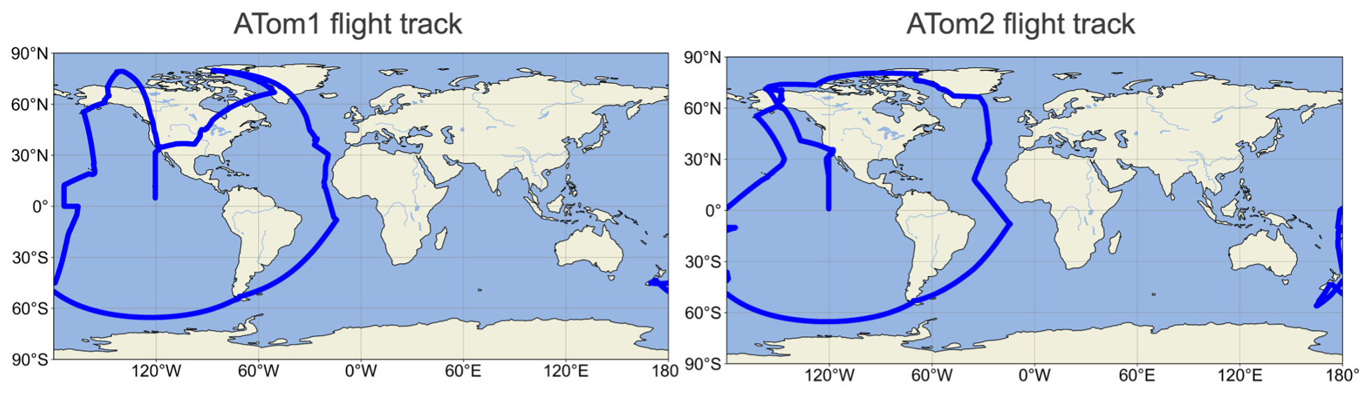
Figure 1 ATom1 and ATom2 flight tracks.

2.3.2 Atmospheric tomography (ATom) aircraft observations

To evaluate the LNO_x emissions calculated by different lightning schemes, we used NO observations by the atmospheric tomography (ATom) aircraft missions (Wofsy et al., 2018). By deploying an extensive gas and aerosol payload on the NASA DC-8 aircraft, ATom is designed to sample the atmosphere systematically on a global scale, performing continuous profiling from 0.2 to 12 km of altitude. Flights took place in each of the four seasons of 2016 through 2018. Since most of the lightning occurs over land regions during summer, ATom1 (July–August 2016) and ATom2 (January–February 2017) were used to evaluate LNO_x emissions (corresponding to summer in the Northern and Southern Hemisphere, respectively). Both ATom1 and ATom2 originate from the Armstrong Flight Research Center in Palmdale, California, USA, fly north to the western Arctic, south to the South Pacific, east to the Atlantic, north to Greenland, and return to California across central North America. Figure 1 exhibits the respective flight tracks of ATom1 and ATom2. To evaluate the model-simulated NO against the ATom observations, we have sampled the specific flight track and timings from the modeled data.

2.3.3 TROPOMI satellite observations

The Tropospheric Monitoring Instrument (TROPOMI) is the payload aboard the Sentinel-5 Precursor (S5P) satellite of the European Space Agency (ESA), which was launched in October 2017. TROPOMI has been providing observations of important atmospheric pollutants (NO₂, O₃, CO, CH₄, SO₂, CH₂O) with an unprecedented horizontal resolution of approximately 7×3.5 km² since August 2017 (changed to 5.5×3.5 km² after August 2019) (Verhoelst et al., 2021). The data used in this study are the TROPOMI level-2 offline (OFFL) tropospheric NO₂ columns in 2019. The product version is 1.0.0 from 1 January to 20 March 2019 updated to 1.1.0 from 21 March to 31 December 2019. For the direct comparisons between TROPOMI level-2 products and CHASER results, the following procedures were conducted to pre-process the TROPOMI data and CHASER modeled fields.

1. The TROPOMI retrievals with quality assurance (QA) values larger than or equal to 0.75 were selected.

2. Horizontally, the TROPOMI data (tropospheric NO₂ columns, temperatures, pressures, averaging kernels) were interpolated to the CHASER 2.8^∘ × 2.8^∘ grid.

3. The modeled results were sampled based on the TROPOMI overpass time. The CHASER tropospheric NO₂ columns were calculated by using the sampled modeled results, the averaging kernels retrieved from the TROPOMI retrievals, and the temperature and pressure profiles provided by TROPOMI retrievals. The averaging kernels are applied to each layer of the CHASER outputs following the Eq. (16).

4. The pre-processed data described above were used to produce the monthly averaged data.

2.3.4 OMI satellite observations

The Ozone Monitoring Instrument (OMI) is a key instrument aboard NASA's Aura satellite for measuring criteria pollutants such as O₃, NO₂, SO₂, and aerosols. OMI has been providing observations with spatial resolution varying from 13 km × 25 km to 26 km × 128 km since October 2004 (Goldberg et al., 2019). The NO₂ product used in this study is the level-3 daily global gridded (0.25^∘ × 0.25^∘) nitrogen dioxide product (OMNO2d) (Krotkov et al., 2019). The O₃ product used in this study is the monthly mean tropospheric column O₃ product developed from OMI in combination with the Aura Microwave Limb Sounder (MLS) with the detailed method described by Ziemke et al. (2006).

2.4 Experiment setup

For this study, all the introduced lightning schemes were implemented into CHASER (MIROC). Six sets of experiments were conducted for this study, and the detailed settings of all experiments are presented in Table 2. For each set of experiments, the same initial conditions and chemical emissions were used except for LNO_x emissions. The set of experiments that applied meteorological nudging also has the same meteorological conditions. The monthly varying soil NO_x emissions used are constant each year for all experiments derived from Yienger and Levy (1995). All experiments used the “backward C-shaped” LNO_x vertical profile (Ott et al., 2010). The LNO_x PE values of IC and CG used in all experiments are set to the same value (250 mol per flash), which is based on the recent literature (Ridley et al., 2005; Cooray et al., 2009; Ott et al., 2010; Allen et al., 2019). It is noteworthy that there are still large uncertainties in determining the LNO_x PE values (Allen et al., 2019; Bucsela et al., 2019), and the choice of different LNO_x PE values may influence the simulated LNO_x emissions and chemical fields. A more sophisticated parameterization of LNO_x PE values needs to be implemented and verified in chemistry–climate models in future research.

The first set of experiments was conducted for the years 2001–2020. It was used to evaluate the distribution of the lightning flash rate against LIS/OTD lightning observations and to derive the historical lightning trend. The second set of experiments is the same as the first set of experiments but uses daily mean LNO_x emission rates of 2001 calculated using lightning schemes for each year. This set of experiments is used to produce results for comparison with those of the first set of experiments to estimate the effects of LNO_x emission trends on tropospheric NO_x and O₃ column trends. The third set of experiments gives results for 2011–2020. These experiments are used to estimate the effects of different lightning schemes on atmospheric chemical fields. To normalize the different annual LNO_x emission amounts by different lightning schemes, temporally and spatially uniform adjustment factors were applied to adjust the mean LNO_x production (2011–2020) to 5.0 Tg N yr⁻¹. Note that the 10-year (2011–2020) mean LNO_x production was adjusted to 5.0 Tg N yr⁻¹, but the LNO_x production in each year is not exactly 5.0 Tg N yr⁻¹. This adjustment was achieved by first conducting the simulations without any adjustment; the 2011–2020 mean LNO_x production ($P_{{\mathrm{LNO}}_x}$) was calculated, and then the corresponding adjustment factor (adj_factor) can be calculated by using the following equation.

$$\begin{array}{}\text{(15)}& \text{adj\_factor}={\displaystyle \frac{\mathrm{5.0}}{P_{{\mathrm{LNO}}_x}}}\end{array}$$

Similarly, we also adjusted the LNO_x emissions in the fourth to the sixth sets of experiments to 5.0 Tg N yr⁻¹. The fourth set of experiments is for 2016, with the fifth set for 2017. These two sets of experiments were conducted to compare model results with ATom1 and ATom2 aircraft observations. The sixth set of experiments is for 2019. It is conducted to evaluate model results using TROPOMI satellite observations.

Table 2 All experiments in this study.

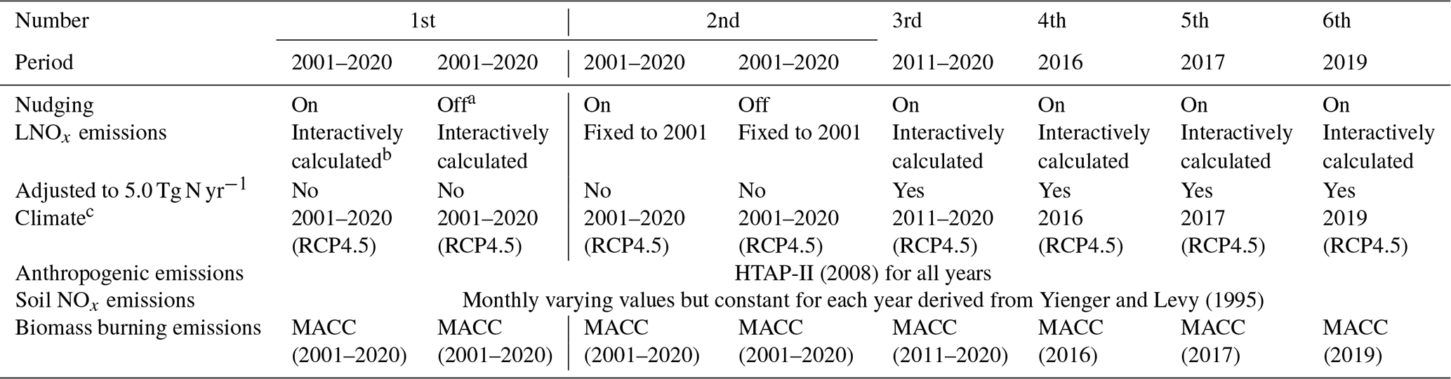
^a Nudging off means the meteorological fields (u, v, T) are free-running instead of nudging towards the NCEP FNL data. ^b LNO_x is interactively calculated by using different lightning schemes. ^c The climate change is simulated by prescribed sea surface temperature (SST) and sea ice fields as well as prescribed varying concentrations of GHGs (CO₂, N₂O, methane, chlorofluorocarbons – CFCs, and hydrochlorofluorocarbons – HCFCs) utilized only in the radiation scheme. The SST and sea ice fields are obtained from the HadISST dataset (Rayner et al., 2003).

3 Results and discussion

3.1 Evaluation of the lightning schemes

As investigated by Finney et al. (2014), 5-year data are necessary and appropriate to produce a lightning climatology. Therefore, model results with nudging (2007–2011) were evaluated against the climatological lightning distributions of LIS (2007–2011) within ±38^∘ latitude and LIS/OTD (1996–2000) within a broader range of ±75^∘ latitude. We have evaluated the potential uncertainties associated with the inconsistency of the time period of simulated lightning and observed lightning (2007–2011 and 1996–2000). The statistical analysis between LIS (2007–2011) and LIS/OTD (1996–2000) within ±38^∘ latitude exhibits an extremely high spatial correlation coefficient (R=0.99) and relatively small relative bias (0.65 %), which supports the reasonability of comparing model results with the observation data within different time ranges.

The distribution of lightning observed by LIS/OTD and simulated by CHASER (MIROC) with different lightning schemes is depicted in Fig. 2. Figure 2 shows that lightning over the ocean is not well reproduced by the original CTH scheme. Actually, it is improved considerably by the new lightning schemes. Compared with the CTH scheme, the original ECMWF scheme better represents the lightning distribution in South Asia including the Indian region. The ECMWF schemes and the ICEFLUX_P scheme reduced negative biases in North America compared to the CTH scheme. In Australia, the ECMWF schemes better simulate the horizontal distribution of lightning. All lightning schemes failed to capture the worldwide maximum value found over the Congo Basin, although all lightning schemes captured the active region in central Africa.

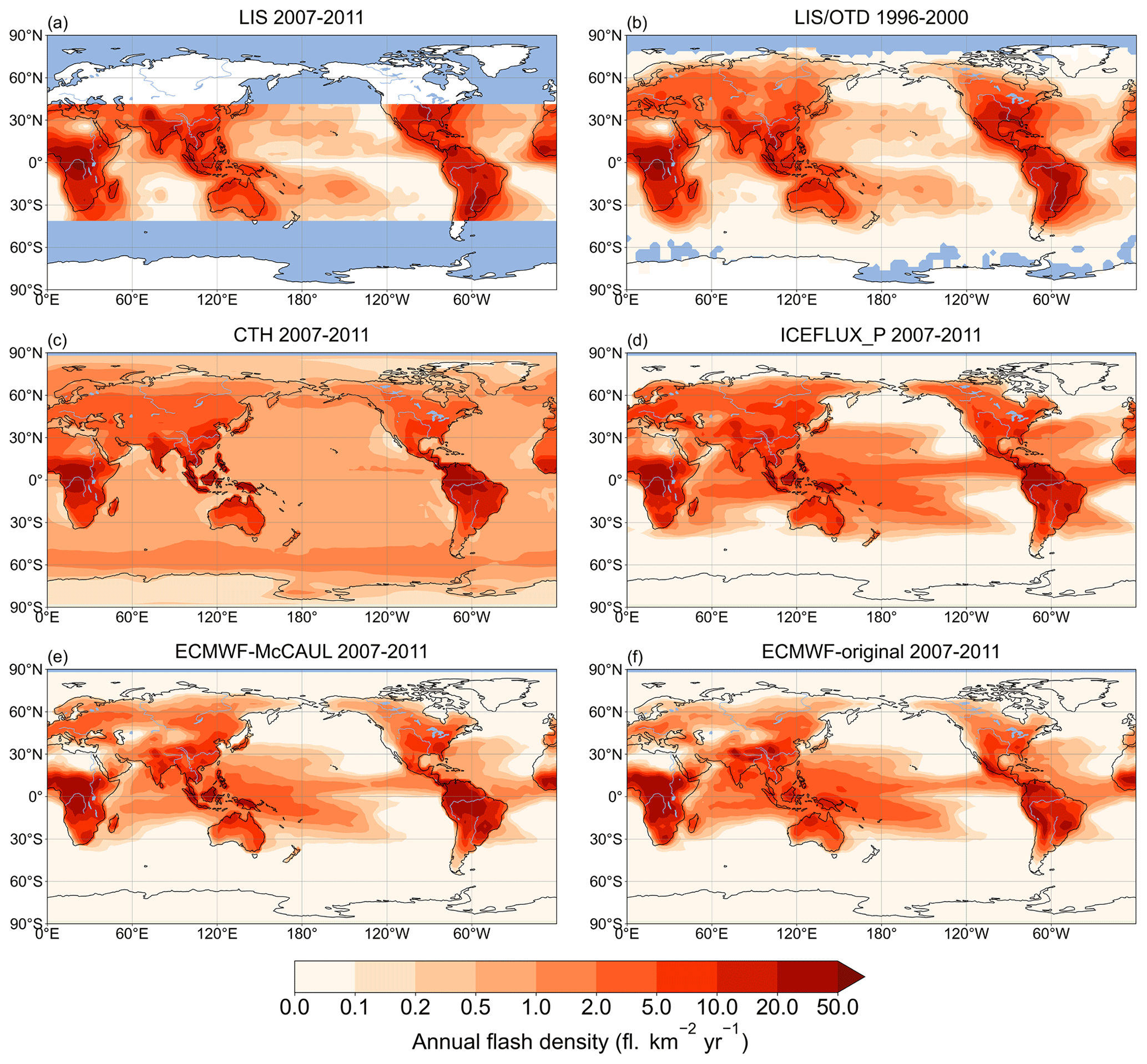
Figure 2 Annual mean lightning flash densities from (a) LIS satellite observations spanning 2007–2011, (b) LIS/OTD satellite observations spanning 1996–2000 but with a wider range, (c) the CTH scheme in 2007–2011, (d) the ICEFLUX_P scheme in 2007–2011, (e) the ECMWF-McCAUL scheme in 2007–2011, and (f) the original ECMWF scheme in 2007–2011.

To directly estimate the prediction accuracy of all lightning schemes, the Taylor diagrams are displayed in Fig. 3. In Fig. 3a, the overall prediction accuracy of the ICEFLUX_P and original ECMWF schemes evaluated against the LIS 2007–2011 lightning climatology is slightly improved compared to the CTH scheme. This improvement is more obvious when considering land and ocean separately (Fig. 3b and c). In the case of Fig. 3a–c, the ECMWF-McCAUL scheme has shown the best prediction accuracy among all lightning schemes. In Fig. 3d, comparison of the annual mean lightning flash rate of LIS/OTD 1996–2000 and the CHASER calculation for 2007–2011 yields spatial correlation coefficients of 0.80 and 0.79 for the ICEFLUX_P and original ECMWF schemes, respectively, which are slightly higher than that found for the CTH scheme (0.78). The overall RMSE of the ICEFLUX_P scheme is 3.32 fl. km⁻² yr⁻¹, which is slightly less than that of the CTH scheme of 3.44 fl. km⁻² yr⁻¹. Among all lightning schemes, the ECMWF-McCAUL scheme exhibits the highest spatial correlation coefficient (0.83) and the lowest RMSE (3.20 fl. km⁻² yr⁻¹) as depicted in Fig. 3d. As displayed in Fig. 2, the prediction accuracy of lightning over the ocean is significantly improved, which can also be verified in Fig. 3f.

Figure 3 Taylor diagram showing the prediction accuracy of various lightning schemes in 2007–2011 simulations compared to the LIS 2007–2011 lightning climatology (a–c) and the LIS/OTD 1996–2000 lightning climatology (d–f).

To estimate whether the improvement of prediction accuracy discussed in Fig. 3 is significant, a significance test is conducted by considering the uncertainties in the LIS/OTD observations. Based on the uncertainties in the LIS/OTD observations, the probability density distributions (PDDs) of spatial correlation coefficients (R) and RMSE between the model and observations are derived by using a Monte Carlo method and displayed in Fig. 4. The uncertainties in the LIS/OTD observations are determined based on the uncertainties of the instrument bulk flash detection efficiency of LIS (88±9 %) and OTD (54±8 %) (Boccippio et al., 2002). The R and RMSE shown in Fig. 4 are all normally distributed, which is determined by the Kolmogorov–Smirnov test. Based on the probability density functions of R and RMSE derived from Fig. 4, the order of R between the model and observations is estimated to be ECMWF-McCAUL > ICEFLUX_P > ECMWF-original > CTH with a confidence limit larger than 99.9 %. Moreover, the order of RMSE between the model and observations is estimated to be ECMWF-McCAUL < ICEFLUX_P < ECMWF-original and CTH with a confidence limit larger than 95 %. According to the significance test described above, we can conclude that the newly implemented lightning schemes have improved the lightning prediction accuracy compared to the original CTH scheme.

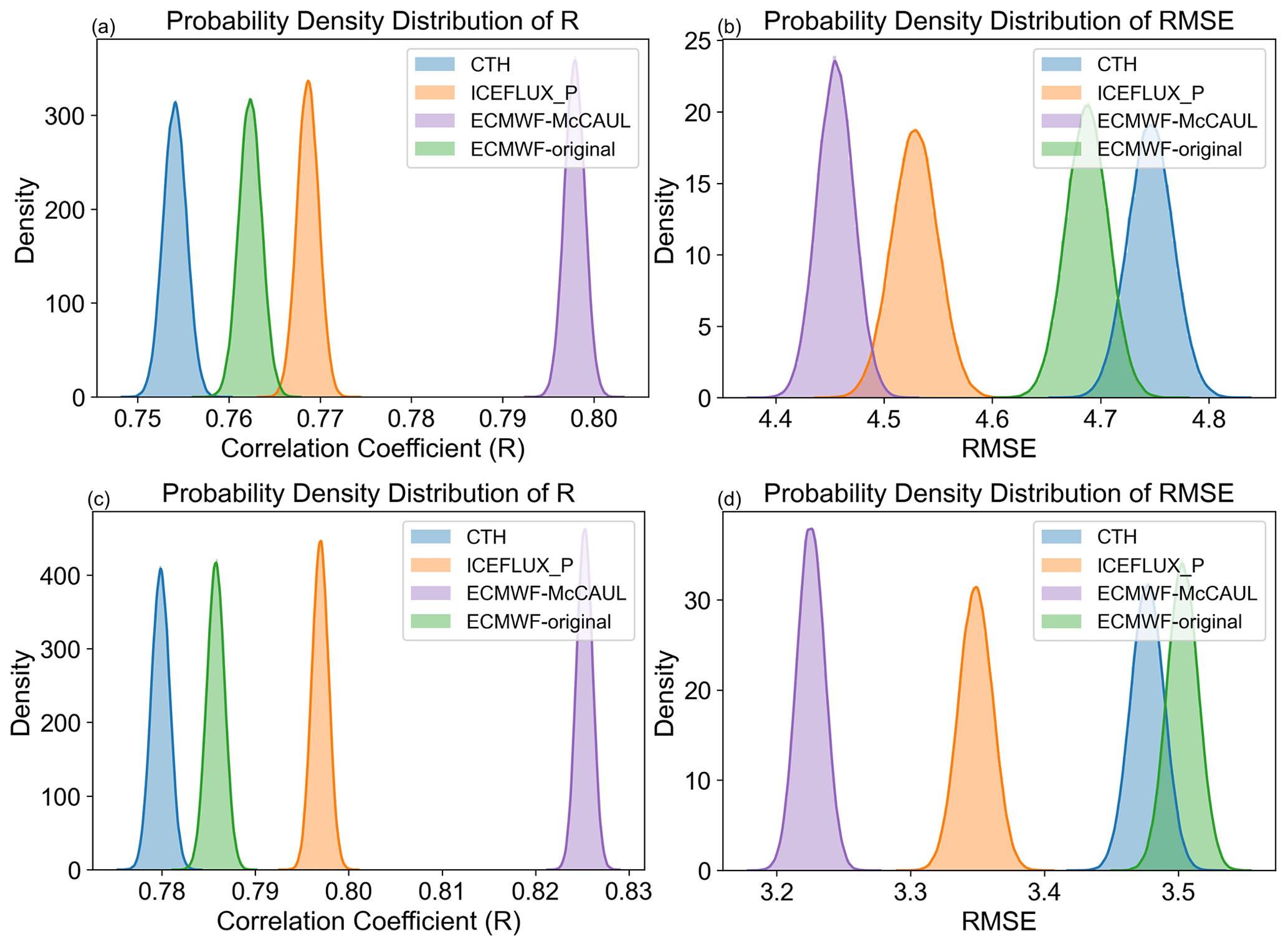
Figure 4 The probability density distributions (PDDs) of spatial correlation coefficients (R) and RMSE between the model and LIS/OTD lightning observations. Panels (a) and (b) show the PDDs obtained between LIS lightning climatology (2007–2011) and the model outputs (2007–2011) within ±38^∘ latitude. Panels (c) and (d) show the PDDs obtained between LIS/OTD lightning climatology (1996–2000) and the model results (2007–2011) within ±75^∘ latitude.

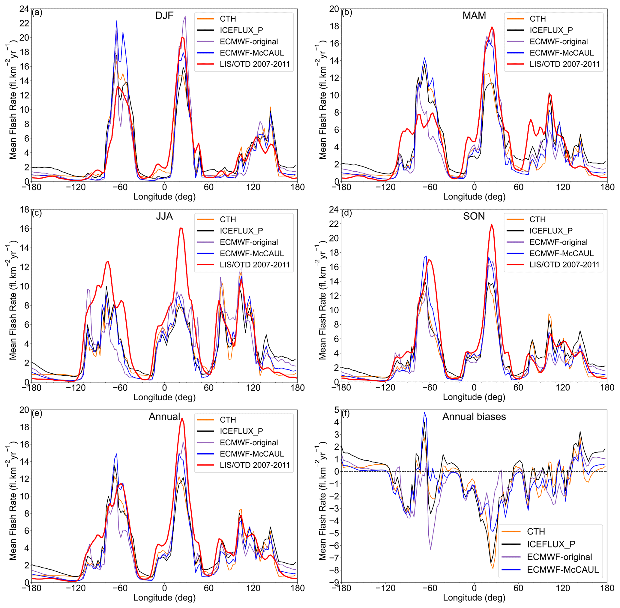
Figure 5 Seasonal and annual meridional average lightning flash density distribution from the LIS 2007–2011 climatology (red line) and from simulation results (2007–2011) obtained using different lightning schemes. The meridional average is only taken within the LIS viewing region of ±38^∘ latitude. The biases (model − obs.) in panel (e) are also portrayed in panel (f).

Figure 5 displays a comparison of seasonal and annual meridional average lightning flash densities from simulations (2007–2011) and LIS satellite observations (2007–2011). As Fig. 5 shows, the pairs of curves are usually in good agreement, even though the annual plot (Fig. 5e) highlights the underestimation which occurs for Africa (from 0 to 30^∘ E) and North America (from 80 to 120^∘ W). The ECMWF schemes have made improvements within Africa. Also, the ICEFLUX_P and the original ECMWF schemes have slightly reduced the biases over North America. A noticeable underestimation over the Americas in JJA and overestimation in MAM can be respectively observed in Fig. 5c and b. Lightning densities over Africa are generally underestimated to varying degrees in different seasons, with the greatest underestimation occurring in JJA (Fig. 5c). Lightning densities over Asia (from 60 to 120^∘ E) are slightly underestimated in MAM (Fig. 5b). The ICEFLUX_P scheme has reduced the biases.

Figure 6 is the same as Fig. 5, but for the zonal mean distributions. The curves of the model results and the observation results in Fig. 6 generally show good agreement. Figure 6f shows that, overall, the ICEFLUX_P and the ECMWF-McCAUL schemes slightly overestimated the lightning densities near the Equator (10^∘ S–10^∘ N). All lightning schemes underestimated the lightning densities within 15–38^∘ N and 20–38^∘ S. Figure 6f also shows that the ICEFLUX_P scheme has reduced the biases within 10–38^∘ N and 15–38^∘ S compared to the CTH scheme. In DJF (Fig. 6a), all lightning schemes overestimated the flash densities over the low-latitude regions but slightly underestimated the flash densities over the middle-latitude regions in the Southern Hemisphere. In MAM (Fig. 6b), lightning densities are overestimated near the Equator and underestimated over 15–38^∘ N and 15–38^∘ S by all lightning schemes to varying degrees. In JJA (Fig. 6c), noticeable overestimation around 10^∘ N by the original ECMWF scheme is apparent. Moreover, the CTH and the original ECMWF schemes respectively facilitated reduction of model biases over 15–38^∘ S and 15–38^∘ N. As Fig. 6d shows, the model-predicted lightning maximum value is shifted approximately 15^∘ to the north in SON compared to the lightning observations. Figure 6d also shows that all lightning schemes underestimated the lightning densities over 15–38^∘ N and 0–38^∘ S. The ICEFLUX_P scheme has shown improvement over these regions.

Figure 6 Seasonal and annual zonal average lightning flash density distribution from the LIS 2007–2011 climatology (red line) and from the simulation results (2007–2011) obtained using different lightning schemes. The biases (model-obs.) in panel (e) are also presented in panel (f).

3.2 Evaluation of LNO_x emissions

3.2.1 Evaluation of LNO_x emissions by ATom1 and ATom2 observations

To evaluate the LNO_x emissions of different lightning schemes, we used ATom1 and ATom2 aircraft measurements (NO) for comparison against model results. All lightning schemes, when implemented in CHASER, produce flash rates corresponding to global annual LNO_x emissions within the range estimated by Schumann and Huntrieser (2007) of 2–8 Tg N yr⁻¹. To eliminate differences in annual total LNO_x emissions by different lightning schemes, we chose to adjust the annual LNO_x emissions of all lightning schemes to 5.0 Tg N yr⁻¹ by applying adjustment factors. The “backward C-shaped” LNO_x vertical profile is applied to all lightning schemes.

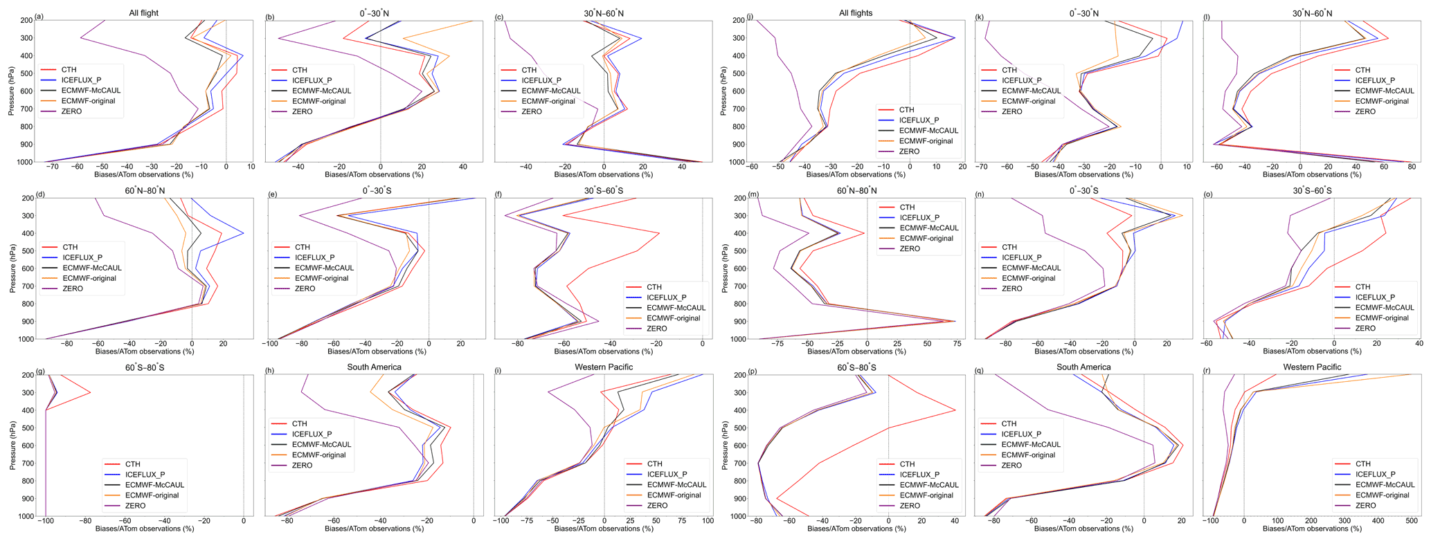
Figure 7 Vertical profile of biases divided by the ATom1 observations (a–i) and the vertical profile of biases divided by the ATom2 observations (j–r). The bias is the model bias (NO) against ATom observations (NO). Data for each pressure level P are calculated within the range of P±50 hPa. South America is the region of 0–30^∘ S, 0–30^∘ W. The western Pacific is the region of 10^∘ N–30^∘ S, 160^∘ E–160^∘ W.

Table 3 Model biases (NO) when compared against ATom1 (a) and ATom2 (b). The unit is parts per trillion (ppt). The biases within the South America region (0–30^∘ S, 0–30^∘ W) and western Pacific region (10^∘ N–30^∘ S, 160^∘ E–160^∘ W) are also shown in this table.

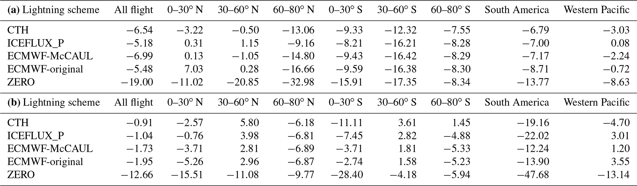
Table 3 presents model biases of different lightning schemes against the ATom1 and ATom2 observations. Figure 7 displays the vertical profile of biases divided by the ATom observations in percentage terms. In Table 3 and Fig. 7, case ZERO is the case with the lightning flash, with LNO_x emissions completely switched off. Comparisons between model results and ATom observations were conducted within two specific regions (South America region and western Pacific region) in which LNO_x is the major source of NO_x (Fig. 8). As Table 3 and Fig. 7 show, the model generally tends to underestimate the NO concentrations. The model biases are reduced considerably by including lightning NO_x sources. For ATom1, overall, the ICEFLUX_P scheme has the smallest model bias. The original ECMWF scheme also reduced the model biases compared to the CTH scheme (Table 3). The ICEFLUX_P and the ECMWF-McCAUL schemes reduced the model biases substantially within 0–30^∘ N latitude where the lightning activities are most dominant during the ATom1 observation period (29 July to 23 August 2016). In the range of 30^∘ S to 80^∘ N in ATom1, overall the ICEFLUX_P scheme reduced the model biases considerably and the ECMWF schemes slightly reduced or extended the model biases compared to the CTH scheme (Table 3, Fig. 7b–e). However, in the range of 30–80^∘ S, the model biases were extended by the ICEFLUX_P and the ECMWF schemes compared to the CTH scheme (Table 3, Fig. 7f and g).

For ATom2, overall, the ECMWF schemes slightly reduced the model biases over the upper troposphere compared to the CTH scheme (Fig. 7j). During the ATom2 observation period (26 January to 21 February 2017), the lightning activities are most dominant within the range of 0–30^∘ S, where the model biases were reduced significantly by newly implemented lightning schemes. A hotspot of lightning activities during the ATom2 observation period is the South America region, where the model biases were reduced dramatically by the ECMWF schemes. The model biases were mostly reduced by the newly implemented lightning schemes within the low-latitude and middle-latitude regions but slightly extended within the high-latitude regions. The model biases were mostly reduced or extended over the middle to upper troposphere (Fig. 7). This is true because most LNO_x was distributed over the middle to upper troposphere. Also, NO_x has a longer lifetime over the middle to upper troposphere. In the western Pacific region, results obtained from comparisons with ATom1 and ATom2 indicate that all lightning schemes overestimated LNO_x emissions in the upper troposphere; also, both the ICEFLUX_P scheme and ECMWF schemes reduced the total model biases considerably more than the CTH scheme did.

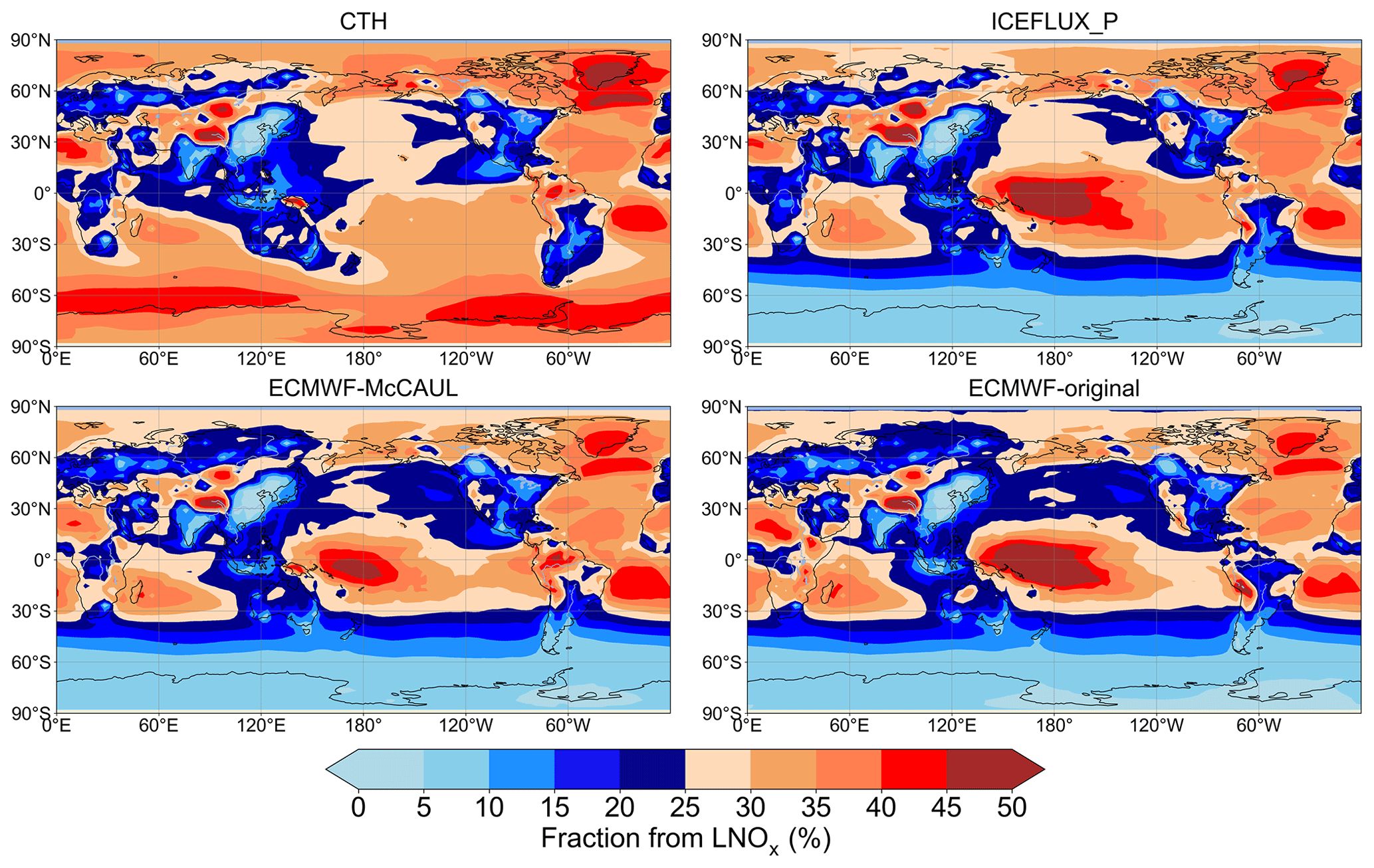
Figure 8 Sensitivity of simulated tropospheric NO₂ columns to LNO_x emissions using different lightning schemes in 2019. NO₂ column because of LNO_x emissions was determined as the difference between the simulation with LNO_x emissions and a simulation that excludes LNO_x emissions.

3.2.2 Evaluation of LNO_x emissions by TROPOMI satellite observations

TROPOMI satellite observations of tropospheric NO₂ columns were used to evaluate LNO_x emission results obtained using the CHASER model. To eliminate differences in annual total LNO_x emissions attributable to the different lightning schemes, we adjusted the annual LNO_x emissions of all lightning schemes to 5.0 Tg N yr⁻¹ using different adjustment factors. For direct comparison between CHASER and TROPOMI tropospheric NO₂ columns, the averaging kernel information from TROPOMI observations was used. The averaging kernels were applied to CHASER outputs following Eq. (16).

$$\begin{array}{}\text{(16)}& X_{\mathrm{chaser}}=\sum _{i=\mathrm{1}}^N{A}_{\mathrm{tropomi}}{x}_{\mathrm{chaser}}\end{array}$$

In that equation, X_chaser represents the CHASER tropospheric NO₂ column after averaging kernels applied, A_tropomi denotes the TROPOMI averaging kernels, x_chaser denotes the CHASER NO₂ partial column at layer i, and N denotes the number of tropospheric layers.

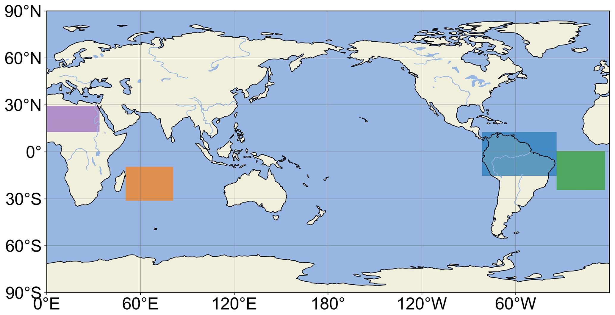
Figure 9 Four target regions for which LNO_x is the major source of NO_x. The four target regions are North Africa (purple), the Indian Ocean (orange), the Amazon (blue), and the South Atlantic (green).

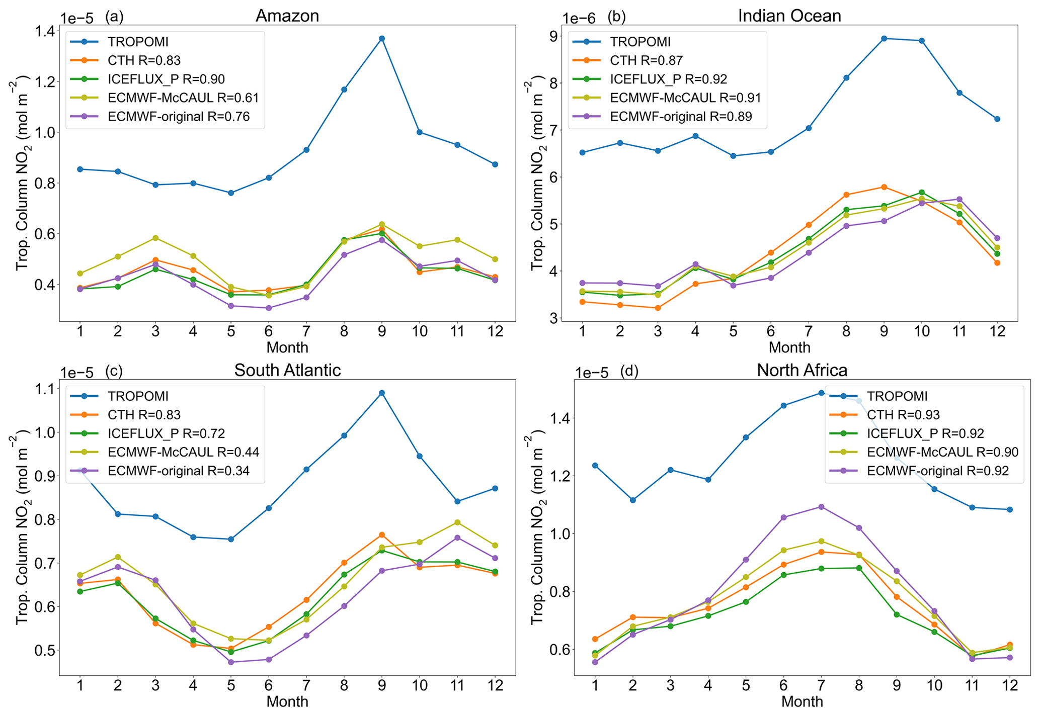
Figure 10 Comparisons of smoothed CHASER and TROPOMI (blue) tropospheric NO₂ columns over four target regions in 2019. Legends show the temporal correlation coefficients.

Comparison between TROPOMI observations and CHASER outputs indicates that the CHASER model tends to underestimate tropospheric NO₂ columns. Overall, the newly implemented lightning schemes have not shown improvements of model biases of tropospheric NO₂ columns at an annual global scale. To minimize the uncertainties of model biases of tropospheric NO₂ columns caused by other factors, we chose to further evaluate the LNO_x emissions by TROPOMI observations over four specific regions (Fig. 9), where LNO_x is the major source of NO_x (as shown in Fig. 8).

Figure 10 presents a comparison of smoothed CHASER and TROPOMI tropospheric NO₂ columns over four target regions in 2019. The spatial average values of each month in 2019 are shown in Fig. 10. That figure shows that the model generally captured the temporal variation of tropospheric NO₂ columns in the four regions. Actually, the temporal variations of modeled tropospheric NO₂ columns are close to each other. For the Amazon region, lightning activities are most dominant during MAM and SON, when the ECMWF-McCAUL scheme has shown noticeable improvements in model biases (Fig. 10a). Figure 10b reveals that all the newly implemented schemes slightly reduced the model biases with the original ECMWF scheme, showing the smallest model biases during the most prevailing season of lighting (DJF). Figure 10c is for the South Atlantic region where the most prevailing season of lighting is also DJF. Figure 10c shows that the ECMWF schemes slightly reduced the model biases compared to the CTH scheme. Referring to Fig. 10d, the dominant season of lightning is JJA, when the ECMWF-original scheme considerably reduced the model biases and the ECMWF-McCAUL scheme also slightly reduced the model biases.

3.3 Effects of different lightning schemes on tropospheric chemical fields

In the tropospheric chemical field, LNO_x has an important role. The LNO_x effects on the tropospheric chemical fields vary along with differences in the horizontal distribution of LNO_x in different lightning schemes. To evaluate the influences of different lightning schemes on the tropospheric chemical fields, several 10-year (2011–2020) experiments were conducted with the 10-year mean LNO_x production of all lightning schemes adjusted to 5.0 Tg N yr⁻¹ (Sect. 2.4). The CTH scheme with a “backward C-shaped” profile is regarded as the base scheme. The effects of different lightning schemes on the atmospheric chemistry are calculated as shown in Eq. (17).

$$\begin{array}{}\text{(17)}& {\mathbf{Impact}}_{ij}={\displaystyle \frac{({\mathbf{LS}}_{ij}-{\mathbf{Base}}_j)}{{\mathbf{Base}}_j}}\end{array}$$

Therein, Impact_ij represents the effects of the ith lightning scheme on the concentrations of target atmospheric component j. Also, LS_ij denotes the concentrations of target atmospheric component j simulated by the ith lightning scheme. Base_j stands for the concentrations of target atmospheric component j as simulated using the base scheme.

Figure 11 presents the respective effects of the ECMWF-McCAUL, original ECMWF, and ICEFLUX_P schemes on the atmospheric chemical fields (NO_x, O₃, OH, CO) relative to the base scheme CTH. The ECMWF-McCAUL scheme led to an increase (approximate maximum is 12 %) in NO_x concentration at low-latitude regions and a decrease (approximate maximum is 15 %) at middle- to high-latitude regions. In the case of the ECMWF-McCAUL scheme, the concentration of ozone and the OH radical mostly increased at low-latitude regions and decreased at middle- to high-latitude regions in the Southern Hemisphere, which corresponds to the changing pattern of NO_x. The effects of the original ECMWF scheme on the atmospheric chemical fields are similar to that of the ECMWF-McCAUL scheme. However, the original ECMWF scheme led to a higher total tropospheric CO burden compared to the ECMWF-McCAUL scheme. As Fig. 11 shows, the three lightning schemes led to a marked decrease in NO_x, O₃, and OH radical concentrations over the South Pole region. This decrease occurred because the lightning densities and the LNO_x emissions simulated by the CTH scheme are markedly higher than those simulated using other lightning schemes at this latitude band (Fig. 2). Moreover, NO_x can engender the formation of ozone and the OH radical. In the case of the ICEFLUX_P scheme, the concentrations of NO_x, ozone, and the OH radical mostly increased in the tropics and decreased at middle- to high-latitude regions in the Southern Hemisphere.

Methane lifetime is an indicator reflecting the tropospheric oxidation capacity. The global mean tropospheric lifetime of methane against the tropospheric OH radical spanning 2011–2020 with the CTH, original ECMWF, ECMWF-McCAUL, and ICEFLUX_P schemes is respectively estimated as 9.226, 9.299, 9.256, and 9.229 years. Compared to the CTH scheme, the ECMWF schemes led to a slight increase in methane's global mean tropospheric lifetime. In contrast, methane's global mean tropospheric lifetime simulated by the ICEFLUX_P scheme is almost the same as that simulated by the CTH scheme. Although little difference exists in the total tropospheric oxidation capacity simulated by different lightning schemes, the ECMWF schemes and ICEFLUX_P scheme led to marked changes in oxidation capacity in different regions of the troposphere.

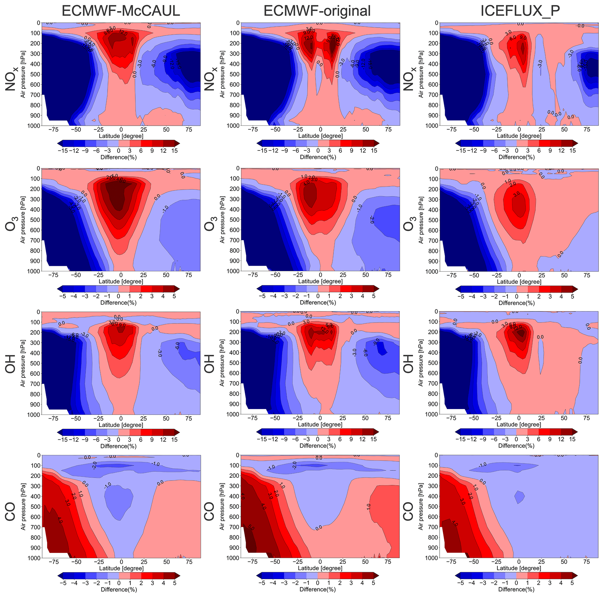
Figure 11 Effects of the ECMWF-McCAUL scheme, original ECMWF scheme, and ICEFLUX_P scheme on the atmospheric chemical fields (NO_x, O₃, OH, CO) relative to the CTH scheme on the zonal mean (%).

3.4 Historical trend analysis of lightning density

The accuracy of predicting the simulated lightning distribution under the current climate is only one aspect of lightning scheme evaluation. The ability of the lightning scheme to reproduce the trend of lightning under climate change is also an important factor. For this study, 20 years of (2001–2020) experiments were conducted to analyze the historical trends of lightning flash rates simulated using different lightning schemes (Sect. 2.4).

Figure 12 Global anomaly of lightning flash rates calculated from simulation results (2001–2020) using different lightning schemes. Panels (a)–(e) present results without nudging; panels (f)–(j) present results with nudging. The grey lines with points represent the monthly time series data on the global mean lightning flash rate anomaly. The blue curves represent the monthly time series data of the global mean lightning flash rate anomaly with the 1-D Gaussian (denoising) filter applied. The red lines are the fitting curves of the grey lines.

Table 4 Changes in global mean surface temperature (ΔTS), global mean lightning flash rate (ΔLFR), and the rate of change in lightning flash rate corresponding to each degree Celsius increase in global mean surface temperature (ΔLFR/ΔTS). Panel (a) shows results obtained without nudging. Panel (b) presents results obtained with nudging. Changes were obtained by calculating the difference between the rightmost and leftmost points of the approximating curve for the 2001–2020 time series data.

Figure 12 shows the global anomaly of lightning flash rates calculated from the simulation results. Because nudging to meteorological reanalysis data cannot be used when predicting lightning trends under future climate changes, we also showed the results without nudging. The un-nudged runs also represented the short-term surface warming like the experiments with nudging. The only differences between the un-nudged and nudged experiments are whether the meteorological fields are nudged towards the 6-hourly NCEP FNL data. We used the Mann–Kendall rank statistic to ascertain whether the lightning trends in Fig. 12 are significant (Hussain and Mahmud, 2019). From results of the Mann–Kendall rank statistic test (significance set as 5 %), all the trends in Fig. 12 were inferred to be significant except for the trends shown in Fig. 12a, e, and i. As Fig. 12 shows, all lightning schemes predicted increasing trends or no significant trends of lightning except the ICEFLUX_P scheme without nudging, which predicted a decreasing lightning trend. The isotherm alternative application of ICEFLUX (ICEFLUX_T) led to slightly enhanced lightning trends toward positive lighting trends compared to the ICEFLUX_P scheme. As explained by Romps (2019), the ICEFLUX_P approach is based on a fixed isobar, which makes it less convenient for climate change studies. Therefore, at least the lightning trends simulated by the ICEFLUX_T approach are expected to be closer to the real situation than the ICEFLUX_P approach.

As displayed in Fig. 12, the positive lightning trends are generally enhanced by application of meteorological nudging. A further investigation of the trends of CAPE during 2001–2020 reveals that the trends of global averaged CAPE are also enhanced by application of meteorological nudging. Higher CAPE means higher buoyancy in the updrafts, which led to the higher lightning densities calculated by the lightning schemes used in this study. It is worth noting that even though the meteorological fields (u, v, T) of nudged simulations are expected to be closer to the real situations, we cannot analogously deduce that the lightning trends predicted by the nudged runs are also closer to the real situations. This is because the predicted lightning trends are not only controlled by the meteorological fields but also controlled by many other physical processes (e.g., cumulus parameterization).

Few studies have specifically examined the lightning trends predicted by the ECMWF schemes under short-term surface warming. When nudging was not applied, the ECMWF schemes predicted the increasing trends of lightning flash rates under short-term surface warming by factors of 4 (ECMWF-McCAUL scheme) and 5 (original ECMWF scheme) compared to the CTH scheme (Table 4).

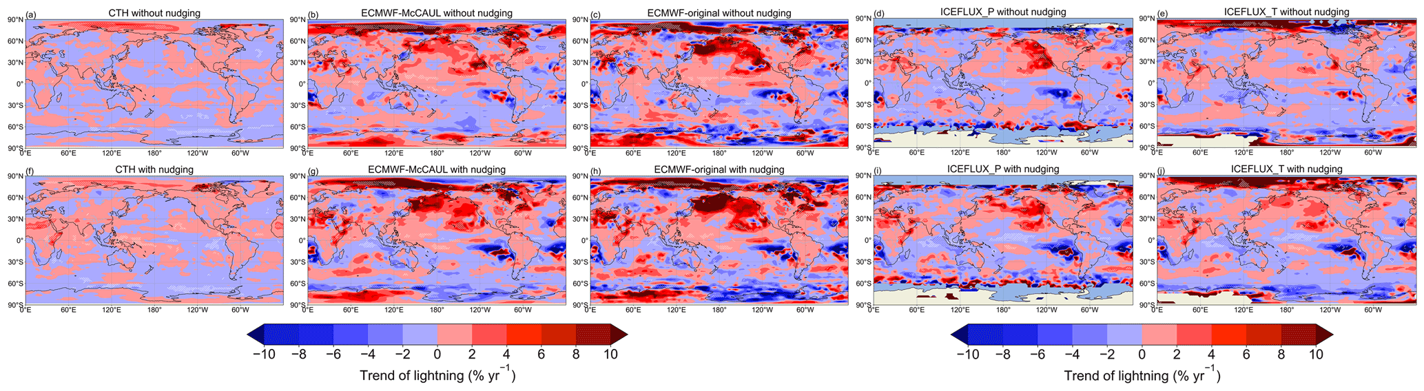
Figure 13 Changes in the lightning flash rate (% yr⁻¹) during 2001–2020 on the two-dimensional map. Changes at every point were calculated from the function of the approximating curve for the 2001–2020 time series data at each grid cell. Panels (a)–(e) show results without nudging; panels (f)–(j) show results with nudging. There are some missing values in the case of the ICEFLUX scheme because the upward cloud ice flux used is diagnosed as zero by the CHASER model, typically within the high-latitude regions.

Figure 13 shows a global map of changes in the lightning flash rate (% yr⁻¹) during 2001–2020. In Fig. 13, the area in which the trend was found to be significant by the Mann–Kendall rank statistic test (significance level inferred for 5 %) is marked with hatched lines. As Fig. 13 shows, the distribution of trends simulated by the same lightning scheme is similar whether meteorological nudging was applied or not. As displayed in Fig. 13, in the Arctic region of the Eastern Hemisphere, both the CTH scheme and the ECMWF schemes showed an increasing trend of lightning. Earlier studies based on the World Wide Lightning Location Network (WWLLN) observations have indicated that lightning densities in the Arctic increase concomitantly with increasing global mean surface temperature (Holzworth et al., 2021). Earlier studies indicate that the results of the CTH scheme and the ECMWF schemes are reasonable for the Arctic region of the Eastern Hemisphere. In the high-latitude region of the Southern Hemisphere (60–70^∘ S), both the CTH scheme and the ECMWF schemes showed decreasing lightning trends. Lightning is rarely observed south of 60^∘ S (Kelley et al., 2018). Moreover, the trends of lightning in this region expected to occur with the short-term surface warming remain highly uncertain. In some parts of the northern Pacific Ocean, the ECMWF schemes and ICEFLUX scheme results showed increasing trends of lightning, which is consistent with results obtained from an earlier study (Petersen and Buechler, 2008). All schemes show decreasing trends for lightning flash rates in Indonesia, although only the ICEFLUX scheme explicitly passed the significance test. In the North Atlantic, all schemes showed increasing lightning trends. Only the CTH scheme failed the significance test.

3.5 Effects of LNO_x emissions on trends of tropospheric O₃ and NO_x columns

The historical trends of lightning densities during 2001–2020 calculated using different lightning schemes have been discussed in Sect. 3.4. Increasing or decreasing trends of lightning can engender corresponding trends of LNO_x emissions, which can consequently influence trends of NO_x and O₃ concentrations. To ascertain the extent to which the LNO_x emissions influence NO_x and O₃ concentration trends, the effects of the LNO_x emissions on the trends of tropospheric NO_x and O₃ columns have been estimated and discussed. We conducted two sets of experiments (Sect. 2.4), one of which interactively calculated LNO_x emission rates, whereas the other one maintained the 2001 LNO_x emission rates for simulations of the entire 20 years. The LNO_x emission effects on the trends of tropospheric NO_x and O₃ columns can be estimated quantitatively by comparing the results of these two sets of experiments. We also conducted the verification of the simulated trends of tropospheric NO_x and O₃ columns by the OMI satellite observations, and the results are exhibited in Figs. S1 and S2. Generally, the model has captured the trends of global averaged tropospheric NO₂ and O₃ columns well even though the trends of both tropospheric NO₂ and O₃ columns are underestimated by the model. Overall, it is obvious that the modeled trends with interannually varying LNO_x emissions with nudging are closest to the OMI observations.

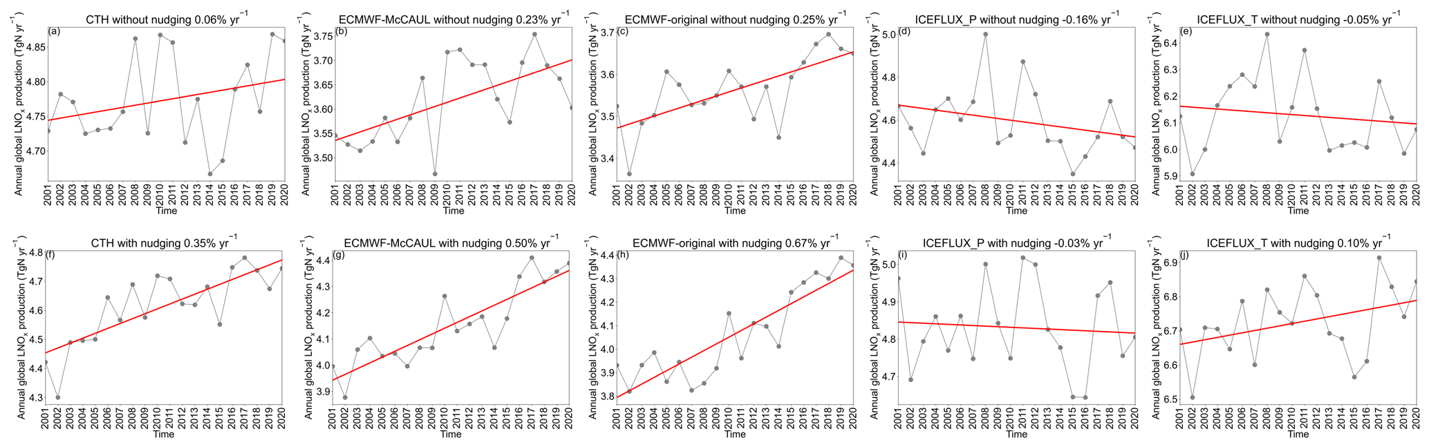
Figure 14 Trends of annual global LNO_x emissions calculated from simulation results (2001–2020) from different lightning schemes. Red lines are fitting curves. Panels (a)–(e) present results without nudging; panels (f)–(j) present results with nudging. The number in the title of each figure represents the trend corresponding to that figure in the unit of percent per year (% yr⁻¹).

Figure 14 presents trends of annual global LNO_x emissions calculated from the simulation results (2001–2020) obtained using different lightning schemes. As Fig. 14 shows, the annual global LNO_x emission trends correspond to the trends of lightning presented in Fig. 12. Similar to the trends found for lightning, the trends of annual global LNO_x emissions are also increased by application of meteorological nudging. Only the ICEFLUX scheme simulated decreasing trends of annual global LNO_x emissions.

Figure 15 Trends of global mean tropospheric NO_x columns calculated from simulation results (2001–2020) using different lightning schemes. Straight lines in the figure are the fitting curves. The numbers in legends represent trends corresponding to that figure in the unit of percent per year (% yr⁻¹). Panels (a)–(e) present results obtained without nudging; panels (f)–(j) present results obtained with nudging.

Figure 15 portrays trends of global mean tropospheric NO_x columns calculated from the first and second set of experiments (Table 2). As Figs. 14 and 15 depict, when the trends of annual global LNO_x emissions are not strong (e.g., Fig. 14a), their effects on the trends of global mean tropospheric NO_x columns are negligible. The marked increasing trends of annual global LNO_x emissions (Fig. 14f–h) led to great increases (12.12 %–20.59 %) of the increasing trends of tropospheric NO_x columns (Fig. 15f–h). In the case of the ICEFLUX_P scheme without nudging, because of the decreasing trends of LNO_x emissions, the increasing trends of the tropospheric NO_x columns decreased by around 10 %.

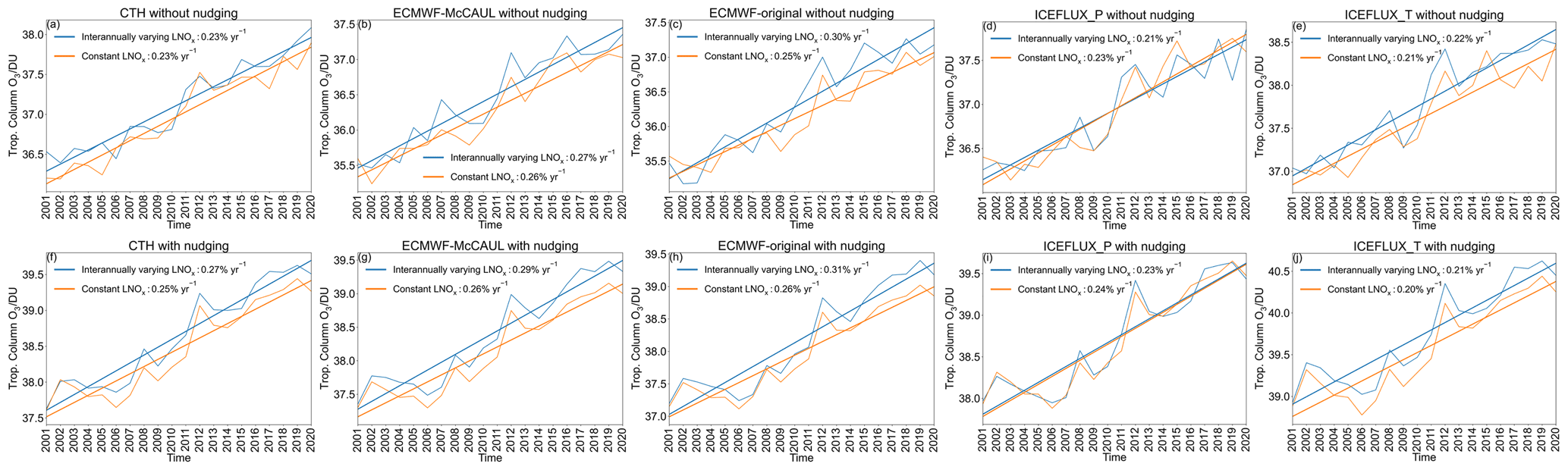
Figure 16 Trends of global mean tropospheric O₃ columns calculated from simulation results (2001–2020) using different lightning schemes. Straight lines in the figure are the fitting curves. The number in the legend represents the trend corresponding to that figure in the unit of percent per year (% yr⁻¹). Panels (a)–(e) present results obtained without nudging; panels (f)–(j) show results obtained with nudging.

Figure 16 is similar to the results shown in Fig. 15, but for tropospheric O₃ columns. Because NO_x causes the formation of O₃ by the fundamental chemical cycle of O_x–NO_x–HO_x, the trends of the global mean tropospheric O₃ columns are strongly affected by trends of the global mean tropospheric NO_x columns. In some cases, the simulated trends of tropospheric O₃ columns are almost identical, as portrayed in Fig. 16a, b, e, i, and j, because the trends of tropospheric NO_x columns simulated by the two sets of experiments are very similar (Fig. 15a, b, e, i, j). As Figs. 14 and 16 show, the marked increasing trends of annual global LNO_x emissions led to increases in the increasing trends of tropospheric O₃ columns by around 15 % (Fig. 16f–h). In the case of ICEFLUX_P without nudging, because of the decreasing trend of LNO_x emissions, the increasing trend of the tropospheric O₃ columns decreased by around 10 % (Fig. 16d). Note that the tropospheric NO_x or O₃ columns in 2001 simulated by the first set of experiments and the second set of experiments are not exactly the same. This is because the blue lines show results with interactively calculated LNO_x emission rates (the time resolution is 10–30 min). But the orange lines show results calculated by reading daily mean input data for LNO_x emission rates, which inhibits interaction of LNO_x with meteorology in the model.

In conclusion, because the ICEFLUX scheme predicts opposite trends of LNO_x emissions from the other lightning schemes, they simulate opposite effects on the historical trends of global mean tropospheric NO_x and O₃ columns. Furthermore, an evident trend of annual global LNO_x emissions has a strong effect on the trend of global mean tropospheric NO_x and O₃ columns.

4 Discussion and conclusions

Three new lightning schemes, the ICEFLUX, the original ECMWF, and the ECMWF-McCAUL schemes, were implemented into CHASER (MIROC), a global chemical climate model. Using LIS/OTD lightning observations as validation data, both the ICEFLUX_P and ECMWF schemes simulated the spatial distribution of lightning more accurately on a global scale than the CTH scheme did, and the lightning distribution in the ocean region was especially improved. The ECMWF-McCAUL scheme showed the highest prediction accuracy for the spatial distribution of lightning on a global scale. It is noteworthy that whilst the ice-based parameterizations showed superb prediction accuracy of lightning distribution under today's climate, they have greater uncertainties associated with inputs, especially regarding the microphysics scheme used (Charn and Parishani, 2021).

To verify the LNO_x emissions of different lightning schemes, we used NO observations from ATom1 and ATom2. Overall, both the ICEFLUX_P scheme and the ECMWF schemes partially reduced model biases, typically over the dominant regions of lightning activities, compared to the CTH scheme. We also used TROPOMI tropospheric NO₂ columns to verify the LNO_x emissions of different lightning schemes. Although the ICEFLUX_P and the ECMWF schemes have not shown improvements of model biases of tropospheric NO₂ columns at an annual global scale, they generally led to an obvious reduction of model biases in the prevailing seasons of lightning within the regions where LNO_x is a dominant source of NO_x. Several studies have pointed out that the TROPOMI data used in this study are biased negatively compared to airborne or ground-based observation data (Tack et al., 2021; Verhoelst et al., 2021; van Geffen et al., 2022). The TROPOMI data used are generally negatively biased and the simulated tropospheric NO₂ columns are underestimated compared to the TROPOMI observations. Therefore, the uncertainties that existed in the TROPOMI data have negligible impacts on the conclusions of our study.

Effects of the newly implemented lightning schemes on the tropospheric chemical fields are evaluated compared to the CTH scheme. Compared with the CTH scheme, the ECMWF schemes mainly led to a slight increase in NO_x, ozone, and OH radical concentrations at low-latitude regions and a decrease at middle-latitude to high-latitude regions. Effects of the ICEFLUX_P scheme on the tropospheric chemical fields slightly differ from those of the ECMWF schemes. The ICEFLUX_P scheme mainly causes a slight increase in NO_x, ozone, and OH radical concentrations from the tropics to the Northern Hemisphere and a decrease in the concentrations of the three chemical species in the Southern Hemisphere except the tropics. The commonality between the ECMWF schemes and the ICEFLUX_P scheme is that they both result in decreasing concentrations of NO_x, ozone, and the OH radical at the middle- to high-latitude regions of the Southern Hemisphere. Although the newly implemented lightning schemes have little effect on the total oxidation capacity of the troposphere compared to the CTH scheme, they led to marked changes in oxidation capacity in different regions of the atmosphere.

This study also analyzed the historical trends of lightning simulated by different lightning schemes under short-term surface warming during 2001–2020. The Mann–Kendall rank statistic was used to ascertain whether the lightning trends were significant. Use of Mann–Kendall rank statistic tests revealed that all the simulated historical lightning trends are significant, except the CTH and ICEFLUX_T schemes without nudging and the ICEFLUX_P scheme with nudging, for significance at 5 %. All the lightning schemes predicted increasing lightning trends or no significant trends except the ICEFLUX_P scheme without nudging, which predicted a decreasing lightning trend. The ICEFLUX_T scheme predicted a decreasing trend without nudging even though the trend failed the significance test. If it is accepted that the non-inductive charging mechanism is an appropriate basis for a lightning parameterization, then the implication is that in the future if cloud ice (and cloud ice fluxes) is reduced then electrical charging will be reduced too. This provides a line of scientific reasoning to explain why lightning may be reduced in the future. Moreover, findings showed that when nudging was not applied, the ECMWF schemes predicted an increasing trend of lightning flash rate under short-term surface warming by factors of 4 (ECMWF-McCAUL scheme) and 5 (original ECMWF scheme) compared to the CTH scheme. Although a considerable degree of uncertainty remains in determining the sensitivity of lightning activity to changes in surface temperature on the decadal timescale (Williams, 2005), the majority of past estimates show that the sensitivity tends average close to 10 % K⁻¹ (Betz et al., 2009, p. 521). This value is most consistent with the lightning increase rate predicted by the ECMWF-McCAUL scheme without nudging in this study. Future research should be undertaken for specific examination of development of lightning schemes that both accurately predict the global distribution of LNO_x and predict the changes in lightning that are expected to occur concomitantly with global climate change. Finally, we quantitatively estimated the LNO_x emission effects on tropospheric NO_x and O₃ column trends during 2001–2020. Results showed that a marked trend of annual global LNO_x emissions significantly affects the trend of global mean tropospheric NO_x and O₃ columns.