the Creative Commons Attribution 4.0 License.
the Creative Commons Attribution 4.0 License.
 | 20 Jul 2022
Computationally efficient methods for large-scale atmospheric inverse modeling
Taewon Cho
Scot M. Miller
Arvind K. Saibaba
Atmospheric inverse modeling describes the process of estimating greenhouse gas fluxes or air pollution emissions at the Earth's surface using observations of these gases collected in the atmosphere. The launch of new satellites, the expansion of surface observation networks, and a desire for more detailed maps of surface fluxes have yielded numerous computational and statistical challenges for standard inverse modeling frameworks that were often originally designed with much smaller data sets in mind. In this article, we discuss computationally efficient methods for large-scale atmospheric inverse modeling and focus on addressing some of the main computational and practical challenges. We develop generalized hybrid projection methods, which are iterative methods for solving large-scale inverse problems, and specifically we focus on the case of estimating surface fluxes. These algorithms confer several advantages. They are efficient, in part because they converge quickly, they exploit efficient matrix–vector multiplications, and they do not require inversion of any matrices. These methods are also robust because they can accurately reconstruct surface fluxes, they are automatic since regularization or covariance matrix parameters and stopping criteria can be determined as part of the iterative algorithm, and they are flexible because they can be paired with many different types of atmospheric models. We demonstrate the benefits of generalized hybrid methods with a case study from NASA's Orbiting Carbon Observatory 2 (OCO-2) satellite. We then address the more challenging problem of solving the inverse model when the mean of the surface fluxes is not known a priori; we do so by reformulating the problem, thereby extending the applicability of hybrid projection methods to include hierarchical priors. We further show that by exploiting mathematical relations provided by the generalized hybrid method, we can efficiently calculate an approximate posterior variance, thereby providing uncertainty information.
- Article
(4262 KB) - Full-text XML
- BibTeX
- EndNote


Numerous satellites and ground-based sensors observe greenhouse gas and air pollution mixing ratios in the atmosphere. A primary goal of atmospheric inverse modeling (AIM) is to estimate emissions or fluxes at the Earth's surface using these observations (Brasseur and Jacob, 2017; Enting, 2002; Michalak et al., 2004; Tarantola, 2005).
The number of greenhouse gas and air pollution measurements has greatly expanded in the past decade, enabling investigations of surface fluxes across larger regions, longer time periods, and/or at finer spatial and temporal detail. Carbon dioxide (CO2) offers an illustrative example. The Greenhouse Gas Observing Satellite (GOSAT), the first satellite dedicated to monitoring CO2 from space, launched in 2009 and collects high-quality observations globally each day (e.g., Nakajima et al., 2012). NASA's Orbiting Carbon Observatory 2 (OCO-2 satellite) launched in 2014 and collects ∼100 times more high-quality observations (Crisp, 2015; Eldering et al., 2017), and upcoming satellites like the Geostationary Carbon Observatory (GeoCarb) could collect up to each day (though some of these observations will likely be unusable due to cloud cover) (Buis, 2018). These new observations are complemented by an expanding ground-based network of observations (NOAA Global Monitoring Laboratory, 2022) and expanded aircraft observations, including partnerships with several airlines to measure atmospheric CO2 from regular commercial flights (Machida et al., 2008; Petzold et al., 2015). In addition, numerous cities are now monitored by dense urban networks of ground-based air sensors (e.g., Shusterman et al., 2016; Davis et al., 2017; Mitchell et al., 2018).
The growing spatial coverage and sheer number of atmospheric GHG observations make it increasingly possible to estimate GHG fluxes in greater spatial and temporal detail; it is key to developing inverse models that can represent all of the information in the observations by estimating emissions at sufficiently high spatiotemporal resolution. In addition, the increasing number of observation networks opens the possibility of rapid monitoring of the carbon cycle and monitoring of changes in anthropogenic emissions – from local to global scales. There is a concomitant need to report realistic uncertainty bounds on these emissions. Arguably, scientists require inverse modeling systems that can be used to estimate emissions and associated uncertainties quickly and at sufficient spatiotemporal resolution to facilitate this broad goal.
However, the computational challenges of achieving these goals are many. First, large-scale inverse models based on Bayesian statistics often require formulation of very large covariance matrices, calculation of matrix–matrix products with those covariance matrices, and/or solution of linear systems with those matrices. Second, existing inverse models often assume a Gaussian prior distribution for use with Bayes' theorem, where the prior mean vector and covariance matrix are required. Statistical approaches to estimating these covariance matrix parameters (e.g., restricted maximum likelihood estimation or Markov chain Monte Carlo methods) are often difficult to implement for extremely large inverse problems (Ganesan et al., 2014; Michalak et al., 2005), and a common approach is to populate the covariance matrices using expert knowledge. Third, fluxes often need to be estimated using iterative optimization algorithms for very large problems, and convergence of these algorithms can be slow (Miller et al., 2020). Fourth, calculating uncertainties in the estimated fluxes can be computationally prohibitive. The design of new methods to improve the computational feasibility of large atmospheric inverse problems has been the focus of numerous recent publications (see, e.g., Baker et al., 2006; Bousserez and Henze, 2018; Chatterjee and Michalak, 2013; Chatterjee et al., 2012; Chen et al., 2021a, b; Gourdji et al., 2012; Henze et al., 2007; Liu et al., 2021; Meirink et al., 2008; Miller et al., 2020, 2014; Yadav and Michalak, 2013; Zammit-Mangion et al., 2021).
Overview of features and contributions
The purpose of this study is to integrate several state-of-the-art computational and mathematical tools with AIM – tools that have been developed for and have had considerable success in other scientific fields (e.g., passive seismic tomography, medical imaging). Specifically, we investigate the use of generalized hybrid (genHyBR) projection methods for surface flux estimation and extend their use for inverse problems where the mean of the fluxes is not known a priori (sometimes referred to as geostatistical inverse modeling) (Chung and Saibaba, 2017; Saibaba et al., 2020). We address these challenges in our present work.
Building on prior work in Miller et al. (2020), we propose a unified computational framework for large-scale AIM with the following features.
-
We describe iterative genHyBR methods that are computationally efficient since they typically converge in a few iterations, are efficient in terms of storage, and work for very large satellite-based inverse problems. For example, we demonstrate the performance of genHyBR methods on two case studies previously considered in Miller et al. (2020). In the larger case study, we solve an inverse problem with 9×10⁶ unknown CO2 fluxes and 1×10⁵ CO2 observations.
-
We extend these methods to handle the case where the mean of the prior distribution is unknown, making genHyBR applicable to a broader range of inverse modeling applications that are common in the atmospheric science community (e.g., geostatistical inverse modeling).
-
Our approach is flexible in that it can be combined with any atmospheric transport model (e.g., either Lagrangian, particle-following models or the adjoint of an Eulerian model), and it can be used with a wide variety of covariance matrices for the unknown parameters and the noise.
-
Our framework also allows for efficiently estimating regularization parameters as part of the reconstruction, thus making it easier to objectively estimate the hyperparameters or covariance matrix parameters as part of the inverse model. We focus on the discrepancy principle (DP), which requires prior knowledge of an estimate of the noise, but provide alternate methods such as the unbiased predictive risk estimator and the generalized cross-validation, the latter of which does not require prior information regarding the noise level.
-
During the solution of the estimates, our solver stores information about the Krylov subspaces that can be used to estimate the posterior variance (at minimal computational cost), which gives insight into the uncertainty in the reconstructed solution. More precisely, evaluating uncertainties does not require additional model evaluations.
An overview of the paper is as follows. In Sect. 2, we describe the problem setup from a Bayesian perspective. In Sect. 3, we describe generalized hybrid methods for atmospheric inverse modeling. We show how to efficiently compute the maximum a posteriori (MAP) estimate and uncertainty estimates (e.g., posterior variance). The focus of this section is on the fixed mean case. We briefly mention an extension to the unknown mean case but defer most of the details to Appendix B. Numerical results are provided in Sect. 4, and conclusions can be found in Sect. 5.
AIM will estimate greenhouse gas fluxes or air pollution emissions that match atmospheric observations, given an atmospheric transport model. It can be represented as an inverse problem of the form
where z∈ℝm is a vector of atmospheric observations, represents the forward atmospheric transport model, s∈ℝn is a vector of the unknown surface fluxes or emissions, and ϵ∈ℝm represents noise or errors, including errors in the atmospheric observations (z) and in the atmospheric transport model (H). Note that s represents a vector containing spatial or spatiotemporal fluxes. Also, we assume , where is a positive definite matrix whose inverse and square root are inexpensive (e.g., a diagonal matrix with positive diagonal entries). The goal of the inverse problem is to estimate s given z and H. The inverse problem may be ill-posed or under-constrained by available observations. Therefore, it is common to include prior information to mitigate the ill-posedness, which is often referred to as variational regularization (Scherzer et al., 2009; Benning and Burger, 2018). We describe two different priors: fixed mean and unknown mean.
2.1 Fixed mean
A common approach in Bayesian inverse modeling is to model s as a Gaussian random variable with a fixed, known mean μ∈ℝn and prior covariance matrix . In many cases, this known mean (μ) is an emissions inventory, a bottom-up flux model, or a process-based model of CO2 fluxes (Brasseur and Jacob, 2017). This approach is also known in the literature as Bayesian synthesis inversion. Using this framework, the prior distribution of s is given as follows:
We assume that matrix Qs is defined by a covariance kernel that describes the spatial and temporal variance and covariance in the prior distribution (Rasmussen and Williams, 2006). Furthermore, λ is a scaling parameter that is known a priori or has to be determined prior to the inversion process. The posterior distribution can be obtained by applying Bayes' theorem , which takes the form
where for any symmetric positive definite matrix M and “∝” denotes a proportionality constant. The MAP estimate corresponding to this posterior distribution can be obtained by solving the optimization problem
Alternatively, it can be computed by solving the system of equations
It is worth mentioning that the resulting posterior distribution is also Gaussian, with mean spost and covariance Qpost, denoted as .
The reconstruction quality of Eq. (1) depends crucially on choosing appropriate covariance matrix parameters, or hyperparameters, that govern this prior Eq. (2) and the noise distribution of ϵ. In Sect. 3.1, we describe genHyBR methods for AIM where μ is fixed but λ is not known in advance.
In many applications, the prior mean μ may also not be known in advance and must be estimated as a part of the inversion process. Some inverse models (commonly referred to as geostatistical inverse models) directly assimilate environmental data or data on emitting activities directly into the inverse model, and the relationships between the surface fluxes and these data are rarely known a priori. In other cases, an emissions inventory or bottom-up flux model may be biased too high or too low. In these cases, Eq. (2) no longer holds, violating the statistical assumptions of the inverse model. One workaround is to scale the inventory or flux model as part of the inverse modeling process, which we now describe.
2.2 Unknown mean
In cases where the prior mean is unknown, we can represent the prior information in the form of the hierarchical model:
Here is a fixed matrix that includes covariates (e.g., environmental data or activity data) or a bottom-up inventory/flux model, is the prior covariance matrix, and λ is a scaling parameter. A set of unknown coefficients β∈ℝp scales the columns of X and is estimated as part of the inverse model. These coefficients are assumed to follow a Gaussian distribution with a given mean μβ∈ℝp, covariance matrix , and scaling parameter λβ.
Given the assumptions in Eqs. (1) and (5), from Bayes' theorem the posterior probability density function for the unknown mean case can be written as
The MAP estimate can be written as the solution of the optimization problem
The posterior distribution in Eq. (6) is Gaussian; therefore, the mean of the posterior distribution is also the MAP estimate, and the covariance is the inverse of the Hessian matrix of Eq. (7) and is given by
Therefore, the resulting posterior distribution is
Here, λ and λβ are scaling parameters that may not be known in advance, but we assume that λβ=αλ with a constant α>0, where α is set in advance. We describe genHyBR methods for the unknown mean case in Sect. 3.3.
Note that previous works (Miller et al., 2020; Saibaba and Kitanidis, 2015) assume an improper prior for β (i.e., p(β)∝1), in which case a solution estimate can be obtained as where
The system in Eq. (9) is often referred to as the dual-function form, and there are several equivalent formulations of these equations (Michalak et al., 2004). The size of the resulting system of equations is , where m is the number of measurements and p is the number of unknown parameters in β, so forming or inverting the matrix in Eq. (9) is unfeasible in many applications. The approach taken in Saibaba and Kitanidis (2012) and Miller et al. (2020) uses a matrix-free iterative method to solve Eq. (9); however, the number of required iterations can be very large, especially for problems with many measurements and even with the use of a preconditioner to speed convergence.
In this paper, we follow a different approach to handle the unknown mean case by using iterative hybrid approaches to a reformulated problem. Since these methods work directly on the least squares problem Eq. (7), the number of unknown parameters is n+p. However, the size of the linear system that defines the MAP estimate is independent of the number of observations, making it attractive for large data sets. Furthermore, our framework can handle a wide class of prior covariance operators, where the resulting prior covariance matrices are large and dense, and explicitly forming and factorizing these matrices is prohibitively expensive. These include, for example, prior covariance matrices that arise from nonseparable, spatiotemporal covariance kernels and parameterized kernels on non-uniform grids. Our approach only relies on forming matrix–vector products with the covariance matrices and is compatible with acceleration techniques using fast Fourier transform (FFT) or hierarchical matrix approaches. See Chung and Saibaba (2017) and Chung et al. (2018) for a detailed discussion. Thus, as we show in Sect. 4, our approach can incorporate various prior models and can scale to very large data sets.
In this section, we describe generalized hybrid projection methods, dubbed genHyBR methods, for AIM. Hybrid projection methods were first developed in the 1980s as a way to combine iterative projection methods (e.g., Krylov subspace methods) and variational regularization methods (e.g., Tikhonov regularization) for solving very large inverse problems. These are iterative methods, where each iteration requires the expansion of the solution subspace, the estimation of the regularization parameter(s), and the solution of a projected, regularized problem. We point the interested reader to survey papers (Chung and Gazzola, 2021; Gazzola and Sabaté Landman, 2020). In Chung and Saibaba (2017), genHyBR methods were developed for computing Tikhonov-regularized solutions to problems where explicit computations of the square root and inverse of the prior covariance matrix are not feasible. This work enabled hybrid projection methods for more general regularization terms. The main benefits of genHyBR methods that make them ideal for large-scale AIM are efficiency, due to fast convergence to an accurate reconstruction of surface fluxes where efficient matrix–vector multiplications are exploited at each iteration, automatic estimation of parameters (e.g., hyperparameters and algorithmic parameters), and flexibility, because they can be paired with many different atmospheric models.
We describe genHyBR methods for both the fixed mean case (Sect. 3.1) and the unknown mean case (Sect. 3.3), with particular emphasis on the associated challenges for large data sets and subsequent uncertainty quantification (UQ) (Sect. 3.2). We provide a general overview of our approach, including the main components of genHyBR methods, in the flowchart in Fig. 1.
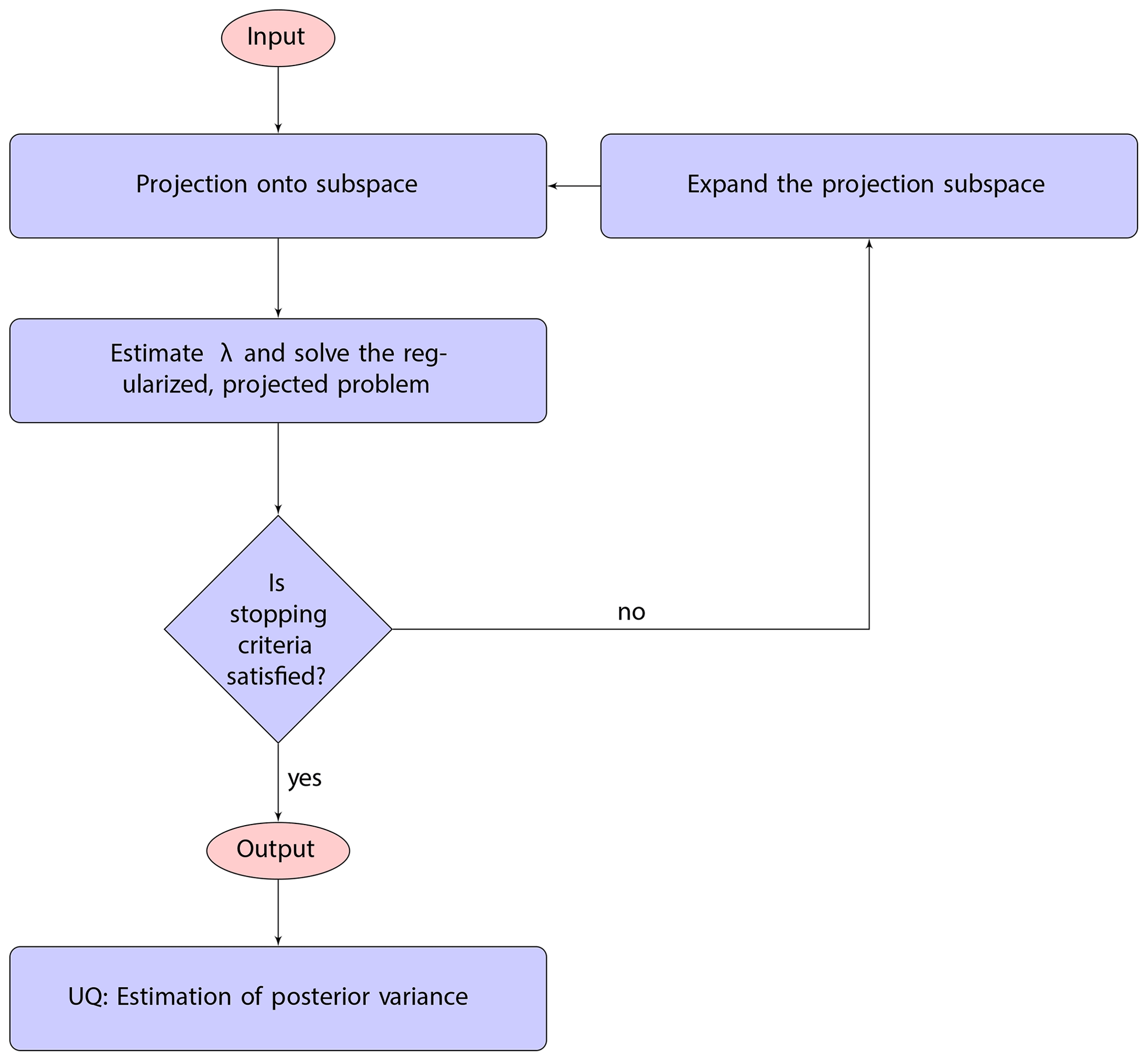
Figure 1This flowchart provides a general overview of using genHyBR methods for AIM and subsequent UQ. Given input (corresponding to the observations and details of the problem setup), genHyBR is an iterative approach to approximate the MAP estimate. Each iteration of genHyBR consists of expanding the solution subspace (Sect. 3.1.1), projecting the problem, estimating a regularization parameter (Sect. 3.1.2), and solving a projected, regularized problem. After obtaining the MAP estimate, information computed from genHyBR can be used to efficiently estimate the posterior variance for UQ (Sect. 3.2).
3.1 Generalized hybrid methods with a fixed mean
To introduce genHyBR methods, we begin with the fixed mean case described in Sect. 2. If symmetric decompositions and are available, then optimization problem Eq. (4) can be rewritten in the standard least squares form
However, computing Ls can be computationally infeasible for large n, and λ may not be known a priori. This motivates us to use the following change in variables,
in which case the solution to problem Eq. (4) is given by , where x solves
Note that, with this reformulation, we avoid Ls, , and and only require matrix–vector products with Qs. Furthermore, for iterative methods for Eq. (11), the matrix H does not need to be formed explicitly, as we only need access to matrix–vector and matrix–transpose–vector products.
There are two main ingredients in the genHyBR approach: (1) the generalized Golub–Kahan bidiagonalization approach for constructing a solution subspace and (2) regularization parameter estimation methods for computing a suitable regularization parameter in the projected space.
3.1.1 Generalized Golub–Kahan bidiagonalization
We now describe the generalized Golub–Kahan bidiagonalization approach that is the backbone of the genHyBR method. Given matrices H, R, and Qs and vector b from Eq. (11), the basic idea is to generate a set of basis vectors contained in Vk for the Krylov subspace:
where ℛ(⋅) denotes the column space and the Krylov subspace is . The generated basis vectors span a low-dimensional subspace that is rich in information about important directions; thus, solutions to the (smaller) projected problem often provide good approximations to the solution of the high-dimensional problem. With initializations , and , the kth iteration of the generalized Golub–Kahan bidiagonalization procedure generates vectors uk+1 and vk+1 such that
where scalars are computed such that . At the end of k iterations, we have
where the following relations hold:
where ej is the jth column of an identity matrix with the appropriate dimensions. Also, matrices Uk+1 and Vk satisfy the following orthogonality conditions:
with . Then, for a given λ>0, the solution to Eq. (11) is recovered by , where yk,λ is the solution to the regularized, projected problem
Note that Eq. (14) is a standard least squares problem with Tikhonov regularization, and since the coefficient matrix Bk is of size , the solution can be computed efficiently (Björck, 1996). Each iteration of the generalized Golub–Kahan bidiagonalization process requires one matrix–vector product with H and its adjoint (suppose we denote its cost by TH), two matrix–vector products with Qs (similarly, denoted ), and additional 𝒪(m+n) floating point operations (flops). To compute the solution of the least squares problem Eq. (14), the cost is 𝒪(k3) flops, and the cost of forming xk,λ is 𝒪(nk) flops. Thus, the overall cost of the algorithm is
In practice, the vectors {uk} and {vk} lose orthogonality in floating point arithmetic, so full or partial re-orthogonalization (Barlow, 2013) can be used to ensure orthogonality. This costs an additional 𝒪(k2(m+n)) flops. Thus far we have described an iterative method for approximating the MAP estimate, Eq. (4), where the kth iterate is given by for fixed regularization parameter λ.
3.1.2 Regularization parameter estimation methods
In this subsection, we highlight one of the main computational benefits of hybrid projection methods, which is the ability to estimate regularization parameters efficiently and adaptively while still ensuring robustness of the solution. For genHyBR approaches, we use the generalized Golub–Kahan bidiagonalization to generate a projection subspace and solve the projected problem Eq. (14) while simultaneously estimating the regularization parameter λ. Note that the regularization term in the projected system (14) is standard Tikhonov regularization, and a plethora of parameter estimation methods exist for Tikhonov regularization (Bardsley, 2018; Hansen, 2010). Here we focus on the discrepancy principle (DP) and point the interested reader to Appendix A for further details on other parameter estimation methods that can be incorporated within genHyBR methods for AIM.
The DP is a common approach for estimating a regularization parameter, where the main goal is to determine λ such that the residual norm for the regularized reconstruction matches a given estimate of the noise level in the observations. That is, the DP method selects the largest parameter value λ for which the reconstructed fluxes sλ satisfy
where τ≥1 is a user-defined parameter and m is the expected value of . Typical choices for safety factor τ are in the range
The DP has been used in AIM (Hase et al., 2017) as well as more generally in inverse problems (Groetsch, 1983; Hansen, 2010). For a given λ, evaluating 𝒟full(λ) requires computation of sλ and matrix–vector multiplication by H, which can get costly if many different values of λ are desired. However, a major distinction here is that by using an iterative hybrid formulation, we can exploit relationships in Eq. (12) for more efficient parameter selection. In particular, the residual norm can be simplified as
Thus, we let λk be the regularization parameter estimated for the projected problem at the kth iteration, such that Then, as the number of iterations k increases, the estimated DP regularization parameter for the projected problem becomes a better approximation of the DP parameter for the original problem.
The advantage of this approach is two-fold: the regularization parameter is selected adaptively (i.e., each iteration can have a different regularization parameter), and the cost of parameter selection is cheap (𝒪(k3) flops) since we work with small matrices of size and k is much smaller than m and n. Furthermore, there are various theoretical results that show that selecting the regularization parameter for the projected problem (i.e., project then regularize) is equivalent to first estimating the regularization parameter and then using an iterative projection method (i.e., regularize then project) (Chung and Gazzola, 2021).
3.2 Approximation to the posterior covariance matrices
In the Bayesian approach for fixed parameter λ, the posterior distribution Eq. (3) is Gaussian and, thus, is fully specified by the mean and covariance matrix. However, neither computing nor storing the covariance matrix is feasible, making further uncertainty estimation challenging. Instead, we follow the approach described in Chung et al. (2018) and Saibaba et al. (2020) for the fixed mean case, where an approximation to the posterior covariance matrix is obtained using the computed vectors generated
during
the generalized Golub–Kahan bidiagonalization process. An advantage of this approach is that, by storing partial information while computing the MAP estimate, we can approximately compute the uncertainty associated with the MAP estimate (e.g., posterior variance) with minimal additional cost and no further access to the forward and adjoint models. For the fixed mean case, we refer to this approach as genHyBRs with UQ and provide a summary in Algorithm 1.
Algorithm 1AIM with fixed mean – genHyBRs with UQ.
In the following, we provide some details regarding the estimation of the posterior variance in the known mean case. This material has previously appeared in Chung et al. (2018, Sect. 4.1), but we provide a brief description here for completeness. An alternative expression for the posterior covariance is
which is obtained by factoring out Qs. This expression is not computationally feasible for large inverse problems but can be approximated using the outputs of the generalized Golub–Kahan bidiagonalization (described in Sect. 3.1.1). After k steps of the generalized Golub–Kahan bidiagonalization approach, we have matrices , and Bk. Let be the eigenvalue decomposition with eigenvalues . Next, we compute the matrix Zk=QsVkWk and the diagonal matrix
Then we can approximate the posterior covariance matrix as
providing an efficient representation of the posterior covariance matrix (as a low-rank perturbation of the prior covariance matrix) that can be used for efficient uncertainty quantification. The accuracy of the approximate posterior covariance matrix and of the resulting posterior distribution can be monitored using the information available from the generalized Golub–Kahan bidiagonalization (Saibaba et al., 2020). Note that in the hybrid approach, we estimate the regularization parameters typically at every iteration; the results in Saibaba et al. (2020) are to be applied after the iterations have been terminated and the regularization parameter has been estimated. The uncertainty estimates therefore depend on the value of the regularization parameter. In general, the approximate posterior variance overestimates the uncertainty and decreases monotonically with the number of iterations k.
To visualize the uncertainty, it is common to compute the diagonals of the posterior covariance (known as the posterior variance). The diagonals of Qs are typically known analytically; the diagonals of the low-rank term can be computed efficiently using Algorithm 2 with input Y=ZkΔk and Z=Zk. An important point worth emphasizing is that the approximation to the posterior covariance need not be computed explicitly. More precisely, in addition to storing the information required for storing Qs, we only need to store nk+k additional entries corresponding to the matrices Zk and Δk.
In addition, one can also use genHyBRs to compute the posterior variance of the sum of the fluxes (or analogously the variance of the mean). To do so, let 1 denote an n×1 vector of ones and multiply the components of as
Several existing studies (Yadav and Michalak, 2013; Miller et al., 2020) describe how to efficiently compute 1⊤Qs1 using Kronecker products.
Note that in previous works (Chung et al., 2018; Saibaba et al., 2020), we found that additional re-orthogonalization of the generalized Golub–Kahan basis vectors yielded more accurate results, so we perform them in the numerical experiments.
Algorithm 2Compute the diagonals of the low-rank term YZ⊤. Call as [d]=LowRankDiag(Y,Z).
3.3 Hierarchical Gaussian priors: reformulation for mean estimation
Next we describe genHyBR methods for AIM with unknown means as described in Sect. 2 with assumptions given in Eq. (5). First, we reformulate the problem for simultaneous estimation of the surface fluxes in s and the covariate parameters in β. Then, we describe how to use genHyBR methods for computing the corresponding MAP estimate Eq. (7) and for subsequent UQ.
We refer to this approach as genHyBRmean with UQ, and since the derivations follow those in Sect. 3.1 and 3.2, specific details have been relegated to Appendix B. However, we would like to emphasize that this derivation is new and a contribution of this work.
Note that optimization problem Eq. (7) can be rewritten in standard least squares form,
if symmetric decompositions and are available. Since computing Ls can be computationally unfeasible (e.g., for spatiotemporal covariance matrices where n is large), we propose a similar change in variables to avoid Ls,
We define the concatenated vector and let , where is included to ensure proper matrix multiplication. Then, optimization problem Eq. (7) can be written as
where
Derivations are provided in Appendix B1. Note that, in practice, neither of the matrices H or K need to be formed explicitly since we only need access to matrix–vector products with these matrices and their transposes. Also, we do not explicitly construct Q but instead provide an efficient way to form matrix–vector products with Q.
In summary, to handle AIM with an unknown mean, the genHyBR method can be used to solve Eq. (18) (as described in Sect. 3.1 with Q instead of Qs, K instead of H, and instead of b) to efficiently obtain the solution . Then, we recover the MAP estimate for s and β as
Similarly to the fixed mean case, we can efficiently approximate the posterior covariance matrix and its diagonals using elements of the generalized Golub–Kahan bidiagonalization algorithm, as described in Appendix B3. We note that efficient UQ approaches for the unknown mean case were considered in Saibaba and Kitanidis (2015), but our approach differs in that we reuse information contained in the subspaces generated during the iterative method rather than randomization techniques, making these derivations straightforward and the approaches widely applicable.
We evaluate the inverse modeling algorithms described in this paper using the two case studies described in Sect. 4.1. For the numerical experiments, we describe the two methods we test.
-
genHyBRsrefers to the fixed mean case and involves solving the optimization problem (4) using the approach described in Sect. 3.1.1 and 3.1.2. -
genHyBRmeanrefers to the unknown mean case and involves solving the optimization problem (18) using the approach described in Sect. 3.3.
For comparison, we use a direct inversion method, which solves Eq. (9) using MATLAB's “backslash” operator. Numerical experiments presented here were obtained using MATLAB on a compute server with four Intel 15-core 2.8 GHz processors and 1 TB of RAM.
4.1 Overview of the case studies
We explore two case studies on estimating CO2 fluxes across North America using observations from NASA's OCO-2 satellite. In the first case study, we estimate CO2 fluxes for 6 weeks (late June through July 2015), an inverse problem that is small enough to estimate using the direct method. The second case study using 1 year of observations (September 2014–August 2015) is too large to estimate directly on many or most computer systems. The goal of these experiments is to demonstrate the performance of the generalized hybrid methods for solving the inverse problem with automatic parameter selection.
The case studies explored here parallel those in Miller et al. (2020) and Liu et al. (2021). We provide an overview of these case studies but refer to Miller et al. (2020) for additional detail on the specific setup. Both of the case studies use synthetic OCO-2 observations that are generated using CO2 fluxes from the NOAA's CarbonTracker product (version 2019b). As a result of this setup, the true CO2 fluxes (s) are known, making it easier to evaluate the accuracy of the algorithms tested here. All atmospheric transport simulations are from the Weather Research and Forecasting (WRF) Stochastic Time-Inverted Lagrangian Transport Model (STILT) modeling system (Lin et al., 2003; Nehrkorn et al., 2010). These simulations were generated as part of the NOAA's CarbonTracker-Lagrange program (Hu et al., 2019; Miller et al., 2020). Note that the WRF-STILT outputs can be used to explicitly construct H, making it straightforward to calculate the direct solution to the inverse problem in the 6-week case study. By contrast, many inverse modeling studies use the adjoint of an Eulerian model. These modeling frameworks rarely produce an explicit H but instead output the product of H or H⊤ and a vector. Though we use WRF-STILT for the case studies presented here, the genHyBR algorithms could also be paired with the adjoint of an Eulerian model.
The goal is to estimate CO2 fluxes at a 3-hourly temporal resolution and a latitude–longitude spatial resolution. Using this modeling framework, synthetic observations were obtained as in Eq. (1) by adding white Gaussian noise (representing measurement and model errors) to the output from the atmospheric transport model. Note that WRF-STILT footprints from CarbonTracker-Lagrange are available at 2 s intervals along the OCO-2 flight track, meaning that there are fewer footprints available than there are observations in the original OCO-2 data files. Indeed, many inverse modeling studies to date have thinned or averaged the OCO-2 observations before assimilating them within an inverse model (e.g., Peiro et al., 2022). We generate the synthetic observations by multiplying CO2 fluxes from CarbonTracker by these footprints, described in greater detail in Miller et al. (2020) and Liu et al. (2021). In total, there are synthetic observations and unknown CO2 fluxes in the 6-week case study. By contrast, for the much larger 1-year case study, there are synthetic observations and unknown CO2 fluxes to be estimated.
The noise covariance matrix is structured as R=σ2I, where σ2 represents the noise variance. In this case, the discrepancy principle formula simplifies to
Note that the DP approach requires a priori knowledge or an estimate of the noise variance σ2. In Miller et al. (2020), σ=2 was used, which leads to a relatively large amount of noise in the observations. We test different values of σ, corresponding to different noise levels (referred to as nlevel), as shown in Table 1. More specifically, let n be a realization of the Gaussian process ; then the amount of noise added in Eq. (1) is ϵ=σn, where . We note that some of the considered noise levels, although very high compared to examples in the inverse problems literature, are lower than typically observed in practice for atmospheric inverse problems. However, recent studies by Miller et al. (2018), O'Dell et al. (2018), Crowell et al. (2019), and Miller and Michalak (2020) show that errors in OCO-2 observations have been gradually decreasing with regular improvements in the satellite retrieval algorithms and bias corrections. Some of the values in Table 1 are low, even considering these recent improvements. With that said, these values are aspirational and may become more realistic in the future as observational and atmospheric modeling errors decline. Furthermore, they provide an opportunity to explore the behavior of the proposed inverse modeling algorithms at many different error levels.
Table 1 Noise level and corresponding noise standard deviation σ used in the 6-week case study experiments.
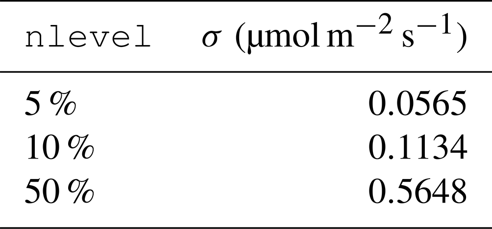
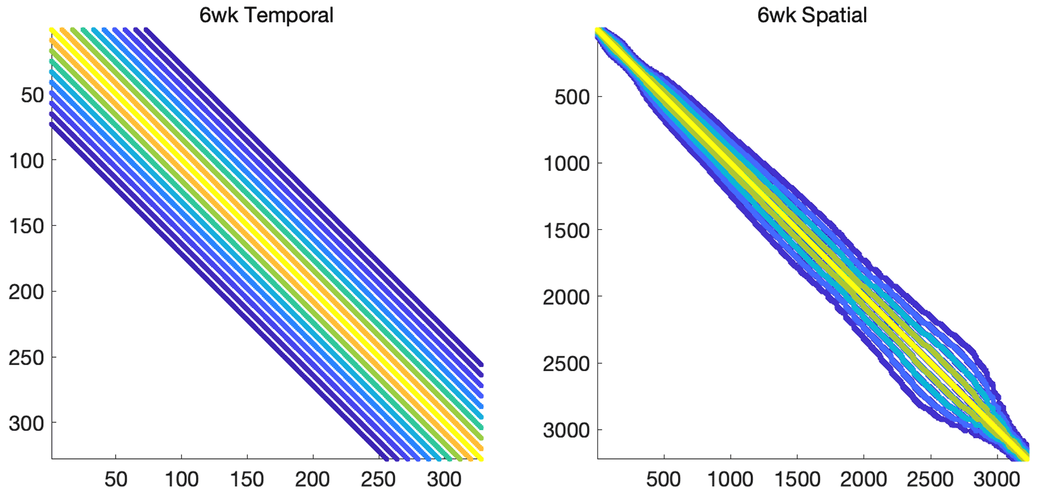
Figure 2Sparsity pattern of the prior covariance matrices Qt and Qg for the 6-week case study.
Next, we describe the prior used in both case studies.
The prior flux estimate is set to a constant value for the case studies explored here. As a result of this setup, the prior flux estimate does not contain any spatiotemporal patterns, and the patterns in the posterior fluxes solely reflect the information content of the atmospheric observations. For the cases with a fixed mean (genHyBRs), we set μ=0, as has been done in several existing studies on inverse modeling algorithms (Rodgers, 2000; Chung and Saibaba, 2017). For the unknown mean case (genHyBRmean), the columns of X contain ones and zeros, denoting fluxes in a given time period.
Specifically, for the 6-week case study, X has eight columns, and each column corresponds to a different 3-hourly time period of the day. A given column of X contains values of one for all flux elements that correspond to a given 3-hourly time of day and zero for all other elements. CO2 fluxes have a large diurnal cycle, and this setup accounts for the fact that CO2 fluxes at different times of day will have a different mean. In the 1-year case study, X has 12 columns, and each column corresponds to fluxes in a different month of the year, a setup identical to that used in Miller et al. (2020).
For the prior covariance matrix of unknown fluxes, , where Qt represents the temporal covariance and Qg represents the spatial covariance in the fluxes. The symbol ⊗ denotes the Kronecker product. We use a spherical covariance model for the spatial and temporal covariance. A spherical model is ideal because it decays to zero at the correlation length or time, and the resulting matrices are usually sparse:
where dt is the temporal difference, dg is the spherical distance, and θt,θg represent the decorrelation time, which has units of d, and decorrelation length, which has units of km, respectively. For the 6-week case study, we set θt=9.854 d and θg=555.42 km, as in Miller et al. (2020). The sparsity patterns of these covariance matrices are provided in Fig. 2. We further set the diagonal elements of Qs equal to one, and the regularization parameter in the inverse model (λ) will ultimately scale Qs (e.g., Eq. 2). For the 1-year study, we use slightly different parameters, as listed in full detail in Miller et al. (2020). Notably, the variance is different in each month to better capture the impact of seasonal changes in the variability of CO2 fluxes. Note that, for the fixed mean case, the covariance matrices are sparse and can be efficiently represented in factored form. However, the hybrid approaches proposed here can handle much more complicated cases (see, e.g., Chung and Saibaba, 2017; Chung et al., 2018).
For the unknown mean case, the covariance matrix Qβ is set to be the identity matrix, and α=10 is used in the numerical experiments. We experimented with various choices for α and observed consistently good results with α=10. In all of the numerical experiments, we use the DP approach to select the regularization parameter within genHyBR methods with τ=1.
In subsequent discussion of the case study results, we provide relative reconstruction error norms computed as , where s denotes the true fluxes and sk,λ contains the reconstructed spatiotemporal fluxes at the kth iteration.
4.2 Results of the case studies
Both the genHyBRs and genHyBRmean methods converge quickly and yield accurate estimates of the CO2 fluxes relative to other inverse modeling methods. For the 6-week case study, Fig. 3 shows the relative reconstruction error norms for both genHyBRs and genHyBRmean for three different noise levels and for different options for selecting the regularization parameter. DP corresponds to the discrepancy principle and is an automatic approach that depends on the data and noise level. The optimal regularization parameter, which corresponds to selecting the regularization parameter at each iteration that minimizes the reconstruction error, is provided for comparison, although it is not obtainable in practice. All of the plots with “none” correspond to λ=0 and show semiconvergent behavior, which is revealed in the “U” shape of the relative error plot. That is, the relative reconstruction error norms decrease in early iterations but increase in later iterations due to noise contamination in the reconstructions.
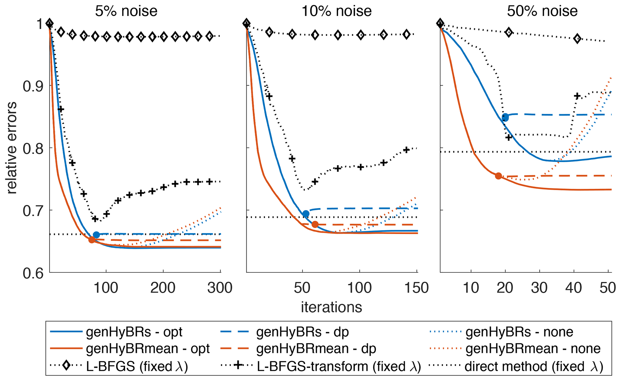
Figure 3Six-week case study: relative reconstruction error norms per iteration of genHyBRs and genHyBRmean with 5 %, 10 %, and 50 % noise levels. We compare results for the optimal regularization parameter, the automatically selected DP parameter, λ=0, and the L-BFGS with a fixed regularization parameter (λ=1). The filled circle indicates the stopping iteration for the genHyBR methods with DP. In addition, the horizontal line denotes to the relative error for the reconstruction obtained using the direct method.
Table 2 Six-week case study: for various noise levels, we provide comparisons of genHyBRs and genHyBRmean (with a DP-selected regularization parameter) to standard direct and iterative methods (with a fixed regularization parameter). We provide the number of iterations, the CPU timing in seconds, and the relative reconstruction error norms for the computed spatiotemporal fluxes denoted by Δs. Note that, when computing the reconstructions and approximating the posterior variance, additional reorthogonalization is performed, which explains the slight difference in the number of iterations and run times.
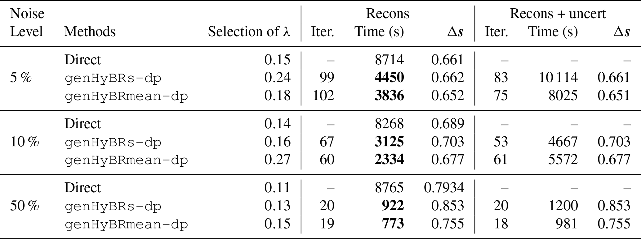
We observe that, for all noise levels, genHyBR methods with regularization parameter estimation (genHyBRs--opt and genHyBRs--dp) result in reconstruction error norms that decrease and flatten, thereby overcoming the semiconvergent behavior of genHyBR methods with no regularization (genHyBRs--none). For reference, we mark with a horizontal line the relative reconstruction error norm for a direct reconstruction. Recall that the direct method and the limited-memory Broyden–Fletcher–Goldfarb–Shanno (L-BFGS) method typically require λ to be fixed in advance, and a poor choice of λ can yield poor reconstructions of the CO2 fluxes. Using the optimal regularization parameter computed from genHyBRmean (these values are provided in Table 2), we show that a good reconstruction can be obtained with the direct method if a good regularization parameter is available, but obtaining this result may require careful and expensive tuning.
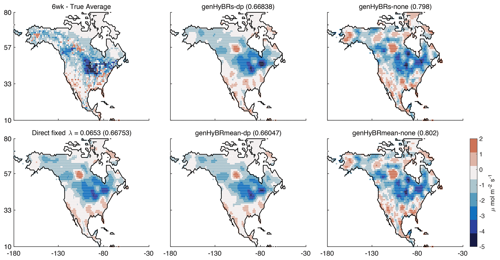
Figure 4Six-week case study: reconstructed fluxes, averaged over 6 weeks, are provided for genHyBRs and genHyBRmean for the automatically selected DP parameter and for λ=0.
The true average fluxes and the reconstruction using a direct method with the optimal regularization parameter computed from genHyBRmean are provided for comparison. These results correspond to the 50 % noise level, and relative error norms of average fluxes over 6 weeks are provided in the titles.

Figure 5Estimated uncertainties for the total CO2 flux from the continental US over the 6-week case study (50 % noise levels). The figure compares posterior uncertainties calculated using the direct approach, using GenHyBR and using the low-rank approach described in Miller et al. (2020). Solid lines show uncertainties estimated for simulations with a fixed mean and dashed lines simulations with an unknown mean. In addition, we use the same regularization parameter (λ) for the estimates shown here to make the convergence behavior of the different approaches easier to compare (λ=0.13 for the fixed mean and λ=0.15 for the unknown mean, as in Table 2). GenHyBR reaches uncertainty estimates that are close to the direct estimate more quickly than the low-rank approach, particularly for the unknown mean case. In addition, GenHyBR uses forward and adjoint model runs previously generated as part of the best estimate calculations, yielding large computational savings over the low-rank approach, which requires new model runs.
We also find that the algorithm that simultaneously estimates the mean (genHyBRmean) yields lower errors than the algorithm with a fixed mean (genHyBRs). Notably, the difference in performance between these two algorithms grows as the noise level increases. In other words, the comparative advantage of genHyBRmean is even larger at higher noise levels. This result implies that mean estimation becomes critical for problems with large noise levels.
For comparison, we show the convergence behavior of the L-BFGS algorithm that is commonly used in AIM (Fig. 3). One line (with diamond symbols) shows results using L-BFGS to minimize the inverse model with an unknown mean (with λ=1), and another line (shown with plus symbols) shows a variant of L-BFGS with a data transformation to speed convergence (also with λ=1). The specific approach used here is described in detail in Miller et al. (2020). Both algorithms converge more slowly than the genHyBR algorithms. This result is significant because the main computational cost per iteration (i.e., one matrix–vector multiplication by H and its adjoint) is the same among the algorithms in Fig. 3. In addition, the relative errors increase for L-BFGS at later iterations, though the inverse modeling optimization function continues to decrease at these iterations; the inverse model minimizes the errors with respect to the observations (z) but is not guaranteed to minimize errors with respect to the true fluxes (s).
The estimated fluxes using genHyBR also exhibit spatial patterns that mirror fluxes estimated using a direct (e.g., analytical) approach. Maps of CO2 fluxes, averaged over 6 weeks and corresponding to a 50 % noise level, are shown in Fig. 4. We provide the true average flux, the genHyBRs and genHyBRmean reconstructions for various parameter choices, and the direct method reconstruction using the optimal regularization parameter from genHyBRmean. Note that these relative reconstruction error values are different than those provided in Fig. 3 because they represent error norms computed on the average image rather than on the native 3 h resolution of the estimated fluxes. Also, to better highlight broad spatial patterns, the color map has been constrained so that average flux estimates above 2 are set to 2 and estimates below −5 are set to −5.
Perhaps surprisingly, the genHyBR algorithms require less computing time than other algorithms tested, including the direct or analytical method. Table 2 displays the measured turnaround time for each case, along with the number of iterations and the relative reconstruction error norms for each method. Compared to the direct method with fixed λ, hybrid methods require less time to compute the estimated CO2 fluxes. Moreover, since the regularization parameter can be selected automatically, genHyBR methods can obtain results with smaller reconstruction errors.
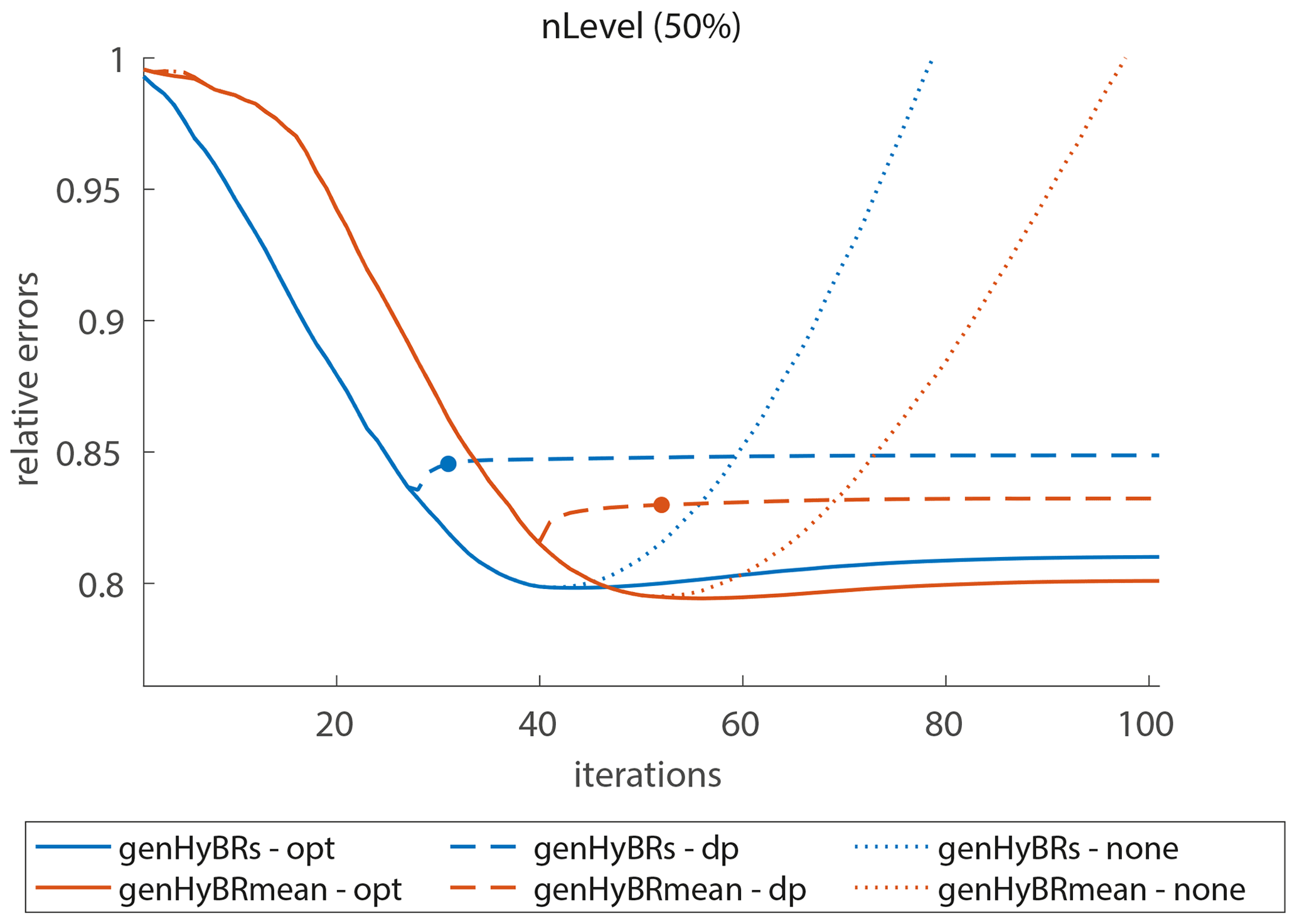
Figure 6One-year case study: for 50 % noise level, we provide relative reconstruction error norms per iteration of genHyBRs and genHyBRmean and compare results for the optimal regularization parameter, the automatically selected DP parameter, and λ=0.
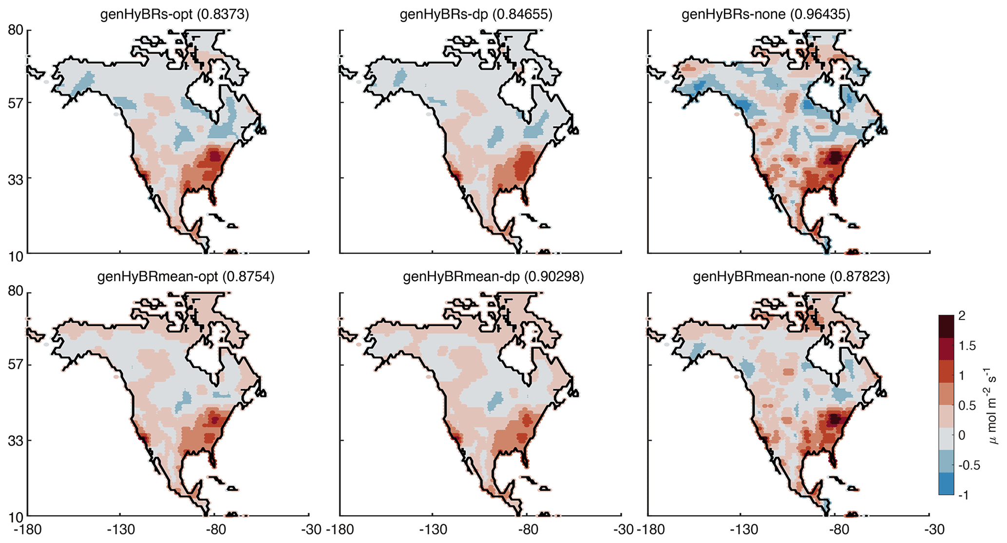
Figure 7One-year case study: reconstructed fluxes, averaged over 1 year, are provided for genHyBRs and genHyBRmean for various parameter choices. These results correspond to the 50 % noise level, and relative error norms of average fluxes over 1 year are provided in the titles.
Finally, we demonstrate the ability to perform UQ for AIM. In the last columns of Table 2, we provide the times needed to compute uncertainties. We remark that the additional time and the difference in the number of iterations can be attributed to the need to perform reorthogonalization of the Krylov basis vectors, which is not as critical for obtaining the MAP estimate. Furthermore, uncertainty estimation for genHyBR does not require any additional forward or adjoint model runs beyond what is required to estimate the fluxes (s). Hence, the additional computing time is modest, given the size of the problem and the ability to obtain solution variance estimates. The estimated posterior variance is also similar across both methods (genHyBRs and genHyBRmean).
GenHyBR also requires relatively few iterations (i.e., Krylov basis vectors) to converge on a reasonable uncertainty estimate. Figure 5 shows the posterior uncertainty in the total continental US CO2 flux by iteration for each algorithm. This figure compares the direct approach to uncertainty estimation, GenHyBR, and the low-rank approach described in Saibaba and Kitanidis (2015) and Miller et al. (2020). In this figure, we use the same regularization parameter (λ) across all algorithms to make the results from different algorithms more easily comparable to one another. The low-rank approach described in Saibaba and Kitanidis (2015) and Miller et al. (2020) starts at very high values and converges more slowly than the uncertainties estimated using GenHyBR. Furthermore, the low-rank approach requires new forward and adjoint runs for the uncertainty calculations, while GenHyBR uses forward and adjoint runs already generated when calculating the best estimate of the fluxes.
We conclude this section with results for the 1-year case study. Since this case study has approximately 9 times the number of unknown CO2 fluxes and 5 times the number of observations compared to the 6-week case study, iterative methods are computationally more appealing than direct methods for obtaining reconstructions. The previous case study already explored the behavior of the algorithms at different noise levels, so here we only consider the 50 % noise level, which corresponds to σ=0.4076. Figure 6 provides relative reconstruction error norms for genHyBRs and genHyBRmean.
With the regularization parameter automatically selected using DP, both methods result in reconstructions with relative errors smaller than 0.85. Since it is difficult to show spatiotemporal flux reconstructions over the entire year, we provide the annual average of the reconstructed CO2 fluxes in Fig. 7.
Compared to the reconstructions in Fig. 4, these average maps are much smoother. This inability to resolve fine details can be attributed to the significantly fewer observations compared to the number of unknowns in this case study. Nevertheless, these results show that the algorithms described in this study can be scaled to very large inverse problems – problems where the direct method is either computationally prohibitive or time-consuming.
This article describes a mathematically advanced iterative method for AIM with large data sets. Specifically, we discuss generalized hybrid methods for inverse models with a fixed prior mean (e.g., Bayesian synthesis inverse modeling) and an unknown prior mean (e.g., geostatistical inverse modeling). We also describe a means of obtaining posterior variance estimates at very little additional computational cost. Compared to standard inverse modeling procedures (e.g., direct and iterative methods), genHyBR methods are computationally cheaper and exhibit faster convergence. One of the main advantages of genHyBR methods is the ability to efficiently and adaptively estimate the regularization parameter during the inversion process, and we described various regularization parameter estimation methods for Tikhonov regularization. Numerical experiments for case studies for 6 weeks and 1 year demonstrate that genHyBR methods provide an efficient, flexible, robust, and automatic approach for AIM with very large spatiotemporal fluxes. Furthermore, since these methods only require forward and adjoint model evaluations, these methods can be paired with different types of atmospheric transport models.
One of the main advantages of hybrid projection methods is the ability to adaptively and automatically estimate the regularization parameter during the iterative process. We described the discrepancy principle (DP), but other common parameter estimation techniques in the context of hybrid projection methods include the generalized cross-validation (GCV) method and the weighted GCV (WGCV) method (Chung et al., 2008; Renaut et al., 2017). A summary of methods with respective functions used to compute the parameters based on the original problem and the projected problem are summarized in Table A1, where for simplicity we have assumed that R=σ2I. We have used the notation for given λ>0, and yk,λ is the solution to the projected problem (14).
Table A1 Regularization parameter selection methods for use within genHyBR methods.
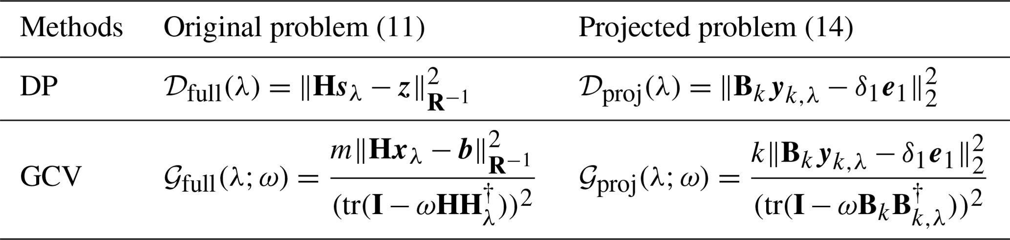
More specifically, DP selects the largest parameter value λ for which 𝒟full(λ)≤τmσ2, where τ≥1 is a user-defined parameter. Note that mσ2 is the expected value of . For the projected problem, we choose the largest λ such that The WGCV method selects λ by minimizing the objective function 𝒢full(λ;ω). Note that, if ω=1, then WGCV becomes GCV. In the projected problem, we minimize 𝒢proj(λ;ω) at each iteration. The parameter ω can be chosen automatically, as described in Chung et al. (2008) and Renaut et al. (2017). Note that the DP approach requires a priori knowledge of the noise variance σ2, whereas GCV approaches do not require prior knowledge about the noise level.
In this section, we provide details for the derivation of genHyBR methods for AIM with an unknown mean. We begin in Appendix B1 with the problem reformulation to simultaneously estimate the unknown fluxes and the covariate parameters. Then in Sect. B2 we provide the details of the genHyBR approach for the unknown mean case, which closely follows the derivation in Sect. 3.1.1. Finally, in Appendix B3 we show how to approximate the posterior variance using the generalized Golub–Kahan bidiagonalization.
B1 Reformulation for simultaneous estimation
In order to apply genHyBR methods to the unknown mean estimation problem, we first reformulate the MAP estimate from Eqs. (7) to (18) as follows. For the data fit term, consider
and for the regularization terms in Eq. (7), we have
We identify , and this completes the derivation of Eq. (18).
Next we provide the derivation of the augmented prior covariance matrix Eq. (19). Since we need Q and not Q−1 in genHyBR, we use the formula for the inverse of a 2×2 block matrix:
which is defined if D and are invertible. Using the above formula, we get
This simplifies to
which completes the derivation of Eq. (19).
B2 genHyBR approach for AIM with an unknown mean
In this subsection, we derive the genHyBR approach for the unknown mean case. We initialize , and ; then, the kth iteration of the generalized Golub–Kahan bidiagonalization procedure generates vectors and such that
where scalars are computed such that . At the end of k iterations, we have
The above matrices satisfy the following relations:
Also, matrices and satisfy the following orthogonality conditions:
The columns of the matrix form a basis for the Krylov subspace , which we use to search for approximate solutions.
To obtain the approximate solution, we solve the least squares problem
to obtain the optimizer and to compute the approximate solution . We can extract the approximations and as . To estimate the regularization parameter, we can adapt the techniques in Sect. 3.1.2; for example, using the discrepancy principle, we pick a regularization parameter λ such that
where τ≥1 is a user-defined parameter and m is the expected value of . Other parameter selection techniques such as GCV and WGCV can also be adapted to the unknown mean case with similar expressions to Table A1, but we omit the details.
B3 Approximation to the posterior variance
We propose an approximation to the posterior covariance matrix Γpost corresponding to the posterior distribution in Eq. (6). First note that, from Eqs. (19) and (8), we get the following expression of the posterior covariance matrix:
where the last expression is obtained by factoring out Q. Assume that k iterations of the generalized Golub–Kahan bidiagonalization have been performed to solve Eq. (18). Let be an eigenvalue decomposition with eigenvalues and let . Then consider the following low-rank approximation:
Using Eq. (B5) in Eq. (B4), we can define an approximate covariance matrix as
where is a diagonal matrix,
The last expression was obtained using the Woodbury formula.
Therefore, we have an efficient representation of the approximate posterior covariance matrix as a low-rank perturbation of the prior covariance matrix Q. It is important to note that, as with the prior covariance matrix Q, we do not need to store explicitly. More precisely, in addition to storing the information required for storing Q, we only need to store nk+k additional entries corresponding to the matrices and . Furthermore, the error in the low-rank approximation can be analyzed using similar techniques to Saibaba et al. (2020). Similar to the approach described in Sect. 3.2, the posterior variance, which corresponds to the diagonal entries of Γpost, can be approximated using the diagonal entries of Eq. (B6). First, note that the diagonals of Q are obtained from the diagonals of the block matrices and α−2Qβ. The diagonals of Qs and Qβ are typically known analytically. The diagonals of XQsX⊤ and are easy to compute in 𝒪((n+p)k2) flops since they are low-rank matrices. Therefore, given the approximate representation of the covariance matrix (B6), we can estimate the posterior variance (i.e., the diagonals of the posterior covariance). A complete description of the method is given in Algorithm B1.
Algorithm B1AIM with unknown mean – genHyBRmean with UQ.
The MATLAB codes for the 6-week case study that were used to generate the results in Sect. 4 are available at https://doi.org/10.5281/zenodo.5772660 (Cho et al., 2021).
The input files for the case study are available on Zenodo at https://doi.org/10.5281/zenodo.3241466 (Miller et al., 2019).
JC, SMM, and AKS designed the study. TC conducted the numerical simulations. All the authors contributed to the writing and presentation of results.
The contact author has declared that none of the authors has any competing interests.
Publisher's note: Copernicus Publications remains neutral with regard to jurisdictional claims in published maps and institutional affiliations.
This work was partially supported by the National Science Foundation ATD program under grant nos. DMS-2026841, DMS-2026830, and DMS-2026835 and by the National Aeronautics and Space Administration under grant no. 80NSSC18K0976. This material was also based upon work partially supported by the National Science Foundation under grant no. DMS-1638521 to the Statistical and Applied Mathematical Sciences Institute. The OCO-2 CarbonTracker-Lagrange footprint library was produced by NOAA/GML and AER Inc with support from NASA Carbon Monitoring System project Andrews (CMS 2014) Regional Inverse Modeling in North and South America for the NASA Carbon Monitoring System. We especially thank Arlyn Andrews, Michael Trudeau, and Marikate Mountain for generating and assisting with the footprint library. Any opinions, findings, and conclusions or recommendations expressed in this material are those of the author(s) and do not necessarily reflect the views of the National Science Foundation.
This research has been supported by the National Science Foundation (grant nos. DMS-2026841, DMS-2026830, DMS-2026835, and DMS-1638521) and by the National Aeronautics and Space Administration under grant no. 80NSSC18K0976.
This paper was edited by Dan Lu and reviewed by two anonymous referees.
Baker, D. F., Doney, S. C., and Schimel, D. S.: Variational data assimilation for atmospheric CO2, Tellus B, 58, 359–365, https://doi.org/10.1111/j.1600-0889.2006.00218.x, 2006. a
Bardsley, J.: Computational Uncertainty Quantification for Inverse Problems, Computer Science and Engineering, SIAM, ISBN 978-1-611975-37-6, 2018. a
Barlow, J. L.: Reorthogonalization for the Golub–Kahan–Lanczos bidiagonal reduction, Numer. Math., 124, 237–278, 2013. a
Benning, M. and Burger, M.: Modern regularization methods for inverse problems, Acta Numer., 27, 1–111, 2018. a
Björck, Å.: Numerical Methods for Least Squares Problems, SIAM, Philadelphia, https://doi.org/10.1137/1.9781611971484, 1996. a
Bousserez, N. and Henze, D. K.: Optimal and scalable methods to approximate the solutions of large-scale Bayesian problems: theory and application to atmospheric inversion and data assimilation, Q. J. Roy. Meteor. Soc., 144, 365–390, https://doi.org/10.1002/qj.3209, 2018. a
Brasseur, G. and Jacob, D.: Modeling of Atmospheric Chemistry, Cambridge University Press, https://doi.org/10.1017/9781316544754, 2017. a, b
Buis, A.: GeoCarb: A New View of Carbon Over the Americas, ExploreEarth, https://www.nasa.gov/feature/jpl/geocarb-a-new-view-of-carbon-over-the-americas (last access: 13 July 2022), 2018. a
Chatterjee, A. and Michalak, A. M.: Technical Note: Comparison of ensemble Kalman filter and variational approaches for CO2 data assimilation, Atmos. Chem. Phys., 13, 11643–11660, https://doi.org/10.5194/acp-13-11643-2013, 2013. a
Chatterjee, A., Michalak, A. M., Anderson, J. L., Mueller, K. L., and Yadav, V.: Toward reliable ensemble Kalman filter estimates of CO2 fluxes, J. Geophys. Res.-Atmos., 117, D22306, https://doi.org/10.1029/2012JD018176, 2012. a
Chen, Z., Liu, J., Henze, D. K., Huntzinger, D. N., Wells, K. C., Sitch, S., Friedlingstein, P., Joetzjer, E., Bastrikov, V., Goll, D. S., Haverd, V., Jain, A. K., Kato, E., Lienert, S., Lombardozzi, D. L., McGuire, P. C., Melton, J. R., Nabel, J. E. M. S., Poulter, B., Tian, H., Wiltshire, A. J., Zaehle, S., and Miller, S. M.: Linking global terrestrial CO2 fluxes and environmental drivers: inferences from the Orbiting Carbon Observatory 2 satellite and terrestrial biospheric models, Atmos. Chem. Phys., 21, 6663–6680, https://doi.org/10.5194/acp-21-6663-2021, 2021a. a
Chen, Z., Huntzinger, D. N., Liu, J., Piao, S., Wang, X., Sitch, S., Friedlingstein, P., Anthoni, P., Arneth, A., Bastrikov, V., Goll, D. S., Haverd, V., Jain, A. K., Joetzjer, E., Kato, E., Lienert, S., Lombardozzi, D. L., McGuire, P. C., Melton, J. R., Nabel, J. E. M. S., Pongratz, J., Poulter, B., Tian, H., Wiltshire, A. J., Zaehle, S., and Miller, S. M.: Five years of variability in the global carbon cycle: comparing an estimate from the Orbiting Carbon Observatory-2 and process-based models, Environ. Res. Lett., 16, 054041, https://doi.org/10.1088/1748-9326/abfac1, 2021b. a
Cho, T., Chung, J., Miller, S. M., and Saibaba, A. K.: Inverse-Modeling/genHyBRmean: Efficient methods for large-scale atmospheric inverse modeling (v1.0), Zenodo [code], https://doi.org/10.5281/zenodo.5772660, 2021. a
Chung, J. and Gazzola, S.: Computational methods for large-scale inverse problems: a survey on hybrid projection methods, arXiv [preprint], arXiv:2105.07221, 2021. a, b
Chung, J. and Saibaba, A. K.: Generalized hybrid iterative methods for large-scale Bayesian inverse problems, SIAM J. Sci. Comput., 39, S24–S46, 2017. a, b, c, d, e
Chung, J., Nagy, J. G., and O’Leary, D. P.: A weighted GCV method for Lanczos hybrid regularization, Electron. T. Numer. Ana., 28, 149–167, 2008. a, b
Chung, J., Saibaba, A. K., Brown, M., and Westman, E.: Efficient generalized Golub–Kahan based methods for dynamic inverse problems, Inverse Probl., 34, 024005, https://doi.org/10.1088/1361-6420/aaa0e1, 2018. a, b, c, d, e
Crisp, D.: Measuring atmospheric carbon dioxide from space with the Orbiting Carbon Observatory-2 (OCO-2), in: Earth Observing Systems XX, edited by: Butler, J. J., Xiong, X. J., and Gu, X., International Society for Optics and Photonics, SPIE, vol. 9607, 1–7, https://doi.org/10.1117/12.2187291, 2015. a
Crowell, S., Baker, D., Schuh, A., Basu, S., Jacobson, A. R., Chevallier, F., Liu, J., Deng, F., Feng, L., McKain, K., Chatterjee, A., Miller, J. B., Stephens, B. B., Eldering, A., Crisp, D., Schimel, D., Nassar, R., O'Dell, C. W., Oda, T., Sweeney, C., Palmer, P. I., and Jones, D. B. A.: The 2015–2016 carbon cycle as seen from OCO-2 and the global in situ network, Atmos. Chem. Phys., 19, 9797–9831, https://doi.org/10.5194/acp-19-9797-2019, 2019. a
Davis, K. J., Deng, A., Lauvaux, T., Miles, N. L., Richardson, S. J., Sarmiento, D. P., Gurney, K. R., Hardesty, R. M., Bonin, T. A., Brewer, W. A., Lamb, B. K., Shepson, P. B., Harvey, R. M., Cambaliza, M. O., Sweeney, C., Turnbull, J. C., Whetstone, J., and Karion, A.: The Indianapolis Flux Experiment (INFLUX): A test-bed for developing urban greenhouse gas emission measurements, Elementa, 5, 21, https://doi.org/10.1525/elementa.188, 2017. a
Eldering, A., Wennberg, P. O., Crisp, D., Schimel, D. S., Gunson, M. R., Chatterjee, A., Liu, J., Schwandner, F. M., Sun, Y., O'Dell, C. W., Frankenberg, C., Taylor, T., Fisher, B., Osterman, G. B., Wunch, D., Hakkarainen, J., Tamminen, J., and Weir, B.: The Orbiting Carbon Observatory-2 early science investigations of regional carbon dioxide fluxes, Science, 358, 6360, https://doi.org/10.1126/science.aam5745, 2017. a
Enting, I.: Inverse Problems in Atmospheric Constituent Transport, Cambridge Atmospheric and Space Science Series, Cambridge University Press, ISBN-13 978-0521018081, ISBN-10 0521018080, 2002. a
Ganesan, A. L., Rigby, M., Zammit-Mangion, A., Manning, A. J., Prinn, R. G., Fraser, P. J., Harth, C. M., Kim, K.-R., Krummel, P. B., Li, S., Mühle, J., O'Doherty, S. J., Park, S., Salameh, P. K., Steele, L. P., and Weiss, R. F.: Characterization of uncertainties in atmospheric trace gas inversions using hierarchical Bayesian methods, Atmos. Chem. Phys., 14, 3855–3864, https://doi.org/10.5194/acp-14-3855-2014, 2014. a
Gazzola, S. and Sabaté Landman, M.: Krylov methods for inverse problems: Surveying classical, and introducing new, algorithmic approaches, GAMM-Mitteilungen, 43, e202000017, https://doi.org/10.1002/gamm.202000017, 2020. a
Gourdji, S. M., Mueller, K. L., Yadav, V., Huntzinger, D. N., Andrews, A. E., Trudeau, M., Petron, G., Nehrkorn, T., Eluszkiewicz, J., Henderson, J., Wen, D., Lin, J., Fischer, M., Sweeney, C., and Michalak, A. M.: North American CO2 exchange: inter-comparison of modeled estimates with results from a fine-scale atmospheric inversion, Biogeosciences, 9, 457–475, https://doi.org/10.5194/bg-9-457-2012, 2012. a
Groetsch, C.: Comments on Morozov’s discrepancy principle, in: Improperly posed problems and their numerical treatment, Springer, 97–104, https://doi.org/10.1007/978-3-0348-5460-3_7, 1983. a
Hansen, P. C.: Discrete Inverse Problems: Insight and Algorithms, SIAM, Philadelphia, https://doi.org/10.1137/1.9780898718836, 2010. a, b
Hase, N., Miller, S. M., Maaß, P., Notholt, J., Palm, M., and Warneke, T.: Atmospheric inverse modeling via sparse reconstruction, Geosci. Model Dev., 10, 3695–3713, https://doi.org/10.5194/gmd-10-3695-2017, 2017. a
Henze, D. K., Hakami, A., and Seinfeld, J. H.: Development of the adjoint of GEOS-Chem, Atmos. Chem. Phys., 7, 2413–2433, https://doi.org/10.5194/acp-7-2413-2007, 2007. a
Hu, L., Andrews, A. E., Thoning, K. W., Sweeney, C., Miller, J. B., Michalak, A. M., Dlugokencky, E., Tans, P. P., Shiga, Y. P., Mountain, M., Nehrkorn, T., Montzka, S. A., McKain, K., Kofler, J., Trudeau, M., Michel, S. E., Biraud, S. C., Fischer, M. L., Worthy, D. E. J., Vaughn, B. H., White, J. W. C., Yadav, V., Basu, S., and van der Velde, I. R.: Enhanced North American carbon uptake associated with El Niño, Sci. Adv., 5, 6, https://doi.org/10.1126/sciadv.aaw0076, 2019. a
Lin, J. C., Gerbig, C., Wofsy, S. C., Andrews, A. E., Daube, B. C., Davis, K. J., and Grainger, C. A.: A near-field tool for simulating the upstream influence of atmospheric observations: The Stochastic Time-Inverted Lagrangian Transport (STILT) model, J. Geophys. Res.-Atmos., 108, 4493, https://doi.org/10.1029/2002JD003161, 2003. a
Liu, X., Weinbren, A. L., Chang, H., Tadić, J. M., Mountain, M. E., Trudeau, M. E., Andrews, A. E., Chen, Z., and Miller, S. M.: Data reduction for inverse modeling: an adaptive approach v1.0, Geosci. Model Dev., 14, 4683–4696, https://doi.org/10.5194/gmd-14-4683-2021, 2021. a, b, c
Machida, T., Matsueda, H., Sawa, Y., Nakagawa, Y., Hirotani, K., Kondo, N., Goto, K., Nakazawa, T., Ishikawa, K., and Ogawa, T.: Worldwide Measurements of Atmospheric CO2 and Other Trace Gas Species Using Commercial Airlines, J. Atmos. Ocean. Tech., 25, 1744–1754, https://doi.org/10.1175/2008JTECHA1082.1, 2008. a
Meirink, J. F., Bergamaschi, P., and Krol, M. C.: Four-dimensional variational data assimilation for inverse modelling of atmospheric methane emissions: method and comparison with synthesis inversion, Atmos. Chem. Phys., 8, 6341–6353, https://doi.org/10.5194/acp-8-6341-2008, 2008. a
Michalak, A. M., Bruhwiler, L., and Tans, P. P.: A geostatistical approach to surface flux estimation of atmospheric trace gases, J. Geophys. Res.-Atmos., 109, D14109, https://doi.org/10.1029/2003JD004422, 2004. a, b
Michalak, A. M., Hirsch, A., Bruhwiler, L., Gurney, K. R., Peters, W., and Tans, P. P.: Maximum likelihood estimation of covariance parameters for Bayesian atmospheric trace gas surface flux inversions, J. Geophys. Res.-Atmos., 110, D24107, https://doi.org/10.1029/2005JD005970, 2005. a
Miller, S. M. and Michalak, A. M.: The impact of improved satellite retrievals on estimates of biospheric carbon balance, Atmos. Chem. Phys., 20, 323–331, https://doi.org/10.5194/acp-20-323-2020, 2020. a
Miller, S. M., Michalak, A. M., and Levi, P. J.: Atmospheric inverse modeling with known physical bounds: an example from trace gas emissions, Geosci. Model Dev., 7, 303–315, https://doi.org/10.5194/gmd-7-303-2014, 2014. a
Miller, S. M., Michalak, A. M., Yadav, V., and Tadić, J. M.: Characterizing biospheric carbon balance using CO2 observations from the OCO-2 satellite, Atmos. Chem. Phys., 18, 6785–6799, https://doi.org/10.5194/acp-18-6785-2018, 2018. a
Miller, S. M., Saibaba, A. K., Trudeau, M. E., Mountain, M. E., and Andrews, A. E.: Geostatistical inverse modeling with large atmo- spheric data: data files for a case study from OCO-2 (Version 1.0), Zenodo [data set], https://doi.org/10.5281/zenodo.3241466, 2019. a
Miller, S. M., Saibaba, A. K., Trudeau, M. E., Mountain, M. E., and Andrews, A. E.: Geostatistical inverse modeling with very large datasets: an example from the Orbiting Carbon Observatory 2 (OCO-2) satellite, Geosci. Model Dev., 13, 1771–1785, https://doi.org/10.5194/gmd-13-1771-2020, 2020. a, b, c, d, e, f, g, h, i, j, k, l, m, n, o, p, q, r, s
Mitchell, L. E., Crosman, E. T., Jacques, A. A., Fasoli, B., Leclair-Marzolf, L., Horel, J., Bowling, D. R., Ehleringer, J. R., and Lin, J. C.: Monitoring of greenhouse gases and pollutants across an urban area using a light-rail public transit platform, Atmos. Environ., 187, 9–23, https://doi.org/10.1016/j.atmosenv.2018.05.044, 2018. a
Nakajima, M., Kuze, A., and Suto, H.: The current status of GOSAT and the concept of GOSAT-2, in: Sensors, Systems, and Next-Generation Satellites XVI, edited by: Meynart, R., Neeck, S. P., and Shimoda, H., International Society for Optics and Photonics, SPIE, vol. 8533, 21–30, https://doi.org/10.1117/12.974954, 2012. a
Nehrkorn, T., Eluszkiewicz, J., Wofsy, S., Lin, J., Gerbig, C., Longo, M., and Freitas, S.: Coupled weather research and forecasting–stochastic time-inverted Lagrangian transport (WRF–STILT) model, Meteorol. Atmos. Phys., 107, 51–64, https://doi.org/10.1007/s00703-010-0068-x, 2010. a
NOAA Global Monitoring Laboratory: Observation sites, https://gml.noaa.gov/dv/site/, last access: 13 July 2022. a
O'Dell, C. W., Eldering, A., Wennberg, P. O., Crisp, D., Gunson, M. R., Fisher, B., Frankenberg, C., Kiel, M., Lindqvist, H., Mandrake, L., Merrelli, A., Natraj, V., Nelson, R. R., Osterman, G. B., Payne, V. H., Taylor, T. E., Wunch, D., Drouin, B. J., Oyafuso, F., Chang, A., McDuffie, J., Smyth, M., Baker, D. F., Basu, S., Chevallier, F., Crowell, S. M. R., Feng, L., Palmer, P. I., Dubey, M., García, O. E., Griffith, D. W. T., Hase, F., Iraci, L. T., Kivi, R., Morino, I., Notholt, J., Ohyama, H., Petri, C., Roehl, C. M., Sha, M. K., Strong, K., Sussmann, R., Te, Y., Uchino, O., and Velazco, V. A.: Improved retrievals of carbon dioxide from Orbiting Carbon Observatory-2 with the version 8 ACOS algorithm, Atmos. Meas. Tech., 11, 6539–6576, https://doi.org/10.5194/amt-11-6539-2018, 2018. a
Peiro, H., Crowell, S., Schuh, A., Baker, D. F., O'Dell, C., Jacobson, A. R., Chevallier, F., Liu, J., Eldering, A., Crisp, D., Deng, F., Weir, B., Basu, S., Johnson, M. S., Philip, S., and Baker, I.: Four years of global carbon cycle observed from the Orbiting Carbon Observatory 2 (OCO-2) version 9 and in situ data and comparison to OCO-2 version 7, Atmos. Chem. Phys., 22, 1097–1130, https://doi.org/10.5194/acp-22-1097-2022, 2022. a
Petzold, A., Thouret, V., Gerbig, C., Zahn, A., Brenninkmeijer, C. A. M., Gallagher, M., Hermann, M., Pontaud, M., Ziereis, H., Boulanger, D., Marshall, J., Nèdèlec, P., Smit, H. G. J., Friess, U., Flaud, J.-M., Wahner, A., Cammas, J.-P., Volz-Thomas, A., and TEAM, I.: Global-scale atmosphere monitoring by in-service aircraft – current achievements and future prospects of the European Research Infrastructure IAGOS, Tellus B, 67, 28452, https://doi.org/10.3402/tellusb.v67.28452, 2015. a
Rasmussen, C. E. and Williams, C.: Gaussian Processes for Machine Learning, the MIT Press, 2, https://doi.org/10.7551/mitpress/3206.001.0001, 2006. a
Renaut, R. A., Vatankhah, S., and Ardestani, V. E.: Hybrid and iteratively reweighted regularization by unbiased predictive risk and weighted GCV for projected systems, SIAM J. Sci. Comput., 39, B221–B243, 2017. a, b
Rodgers, C. D.: Inverse Methods for Atmospheric Sounding: Theory and Practice, vol. 2, World scientific, https://doi.org/10.1142/3171, 2000. a
Saibaba, A. K. and Kitanidis, P. K.: Efficient methods for large-scale linear inversion using a geostatistical approach, Water Resour. Res., 48, W05522, https://doi.org/10.1029/2011WR011778, 2012. a
Saibaba, A. K. and Kitanidis, P. K.: Fast computation of uncertainty quantification measures in the geostatistical approach to solve inverse problems, Adv. Water Resour., 82, 124–138, https://doi.org/10.1016/j.advwatres.2015.04.012, 2015. a, b, c, d
Saibaba, A. K., Chung, J., and Petroske, K.: Efficient Krylov subspace methods for uncertainty quantification in large Bayesian linear inverse problems, Numer. Linear Algebr., 27, e2325, https://doi.org/10.1002/nla.2325, 2020. a, b, c, d, e, f
Scherzer, O., Grasmair, M., Grossauer, H., Haltmeier, M., and Lenzen, F.: Variational methods in imaging, https://doi.org/10.1007/978-0-387-69277-7_8, 2009. a
Shusterman, A. A., Teige, V. E., Turner, A. J., Newman, C., Kim, J., and Cohen, R. C.: The BErkeley Atmospheric CO2 Observation Network: initial evaluation, Atmos. Chem. Phys., 16, 13449–13463, https://doi.org/10.5194/acp-16-13449-2016, 2016. a
Tarantola, A.: Inverse Problem Theory and Methods for Model Parameter Estimation, Other Titles in Applied Mathematics, SIAM, https://doi.org/10.1137/1.9780898717921, 2005. a
Yadav, V. and Michalak, A. M.: Improving computational efficiency in large linear inverse problems: an example from carbon dioxide flux estimation, Geosci. Model Dev., 6, 583–590, https://doi.org/10.5194/gmd-6-583-2013, 2013. a, b
Zammit-Mangion, A., Bertolacci, M., Fisher, J., Stavert, A., Rigby, M. L., Cao, Y., and Cressie, N.: WOMBAT: A fully Bayesian global flux-inversion framework, arXiv [preprint], arXiv:2102.04004, 2021. a
- Abstract
- Introduction
- Bayesian approach to inverse modeling
- Generalized hybrid projection methods for AIM
- Numerical results
- Conclusions
- Appendix A: Regularization parameter estimation methods for genHyBR
- Appendix B: Extension to the unknown mean: hierarchical Bayes
- Code availability
- Data availability
- Author contributions
- Competing interests
- Disclaimer
- Acknowledgements
- Financial support
- Review statement
- References