the Creative Commons Attribution 4.0 License.
the Creative Commons Attribution 4.0 License.
 | 18 Jul 2022
Block-structured, equal-workload, multi-grid-nesting interface for the Boussinesq wave model FUNWAVE-TVD (Total Variation Diminishing)
Young-Kwang Choi
Fengyan Shi
Matt Malej
Jane M. Smith
James T. Kirby
Stephan T. Grilli
We describe the development of a block-structured, equal-CPU-load (central processing unit), multi-grid-nesting interface for the Boussinesq wave model FUNWAVE-TVD (Fully Nonlinear Boussinesq Wave Model with Total Variation Diminishing Solver). The new model framework does not interfere with the core solver, and thus the core program, FUNWAVE-TVD, is still a standalone model used for a single grid. The nesting interface manages the time sequencing and two-way nesting processes between the parent grid and child grid with grid refinement in a hierarchical manner. Workload balance in the MPI-based (message passing interface) parallelization is handled by an equal-load scheme. A strategy of shared array allocation is applied for data management that allows for a large number of nested grids without creating additional memory allocations. Four model tests are conducted to verify the nesting algorithm with assessments of model accuracy and the robustness in the application in modeling transoceanic tsunamis and coastal effects.
- Article
(17696 KB) - Full-text XML
- BibTeX
- EndNote


To improve the resilience of the world's highly populated coastal areas to tsunami hazard when tsunamigenic events (typically earthquakes or landslides) occur, there has been an increasing need for issuing early warnings and near- and far-field forecasts of tsunami coastal impact. This has led to a growing demand for accurate and efficient models of transoceanic tsunami propagation, in multiple-level nested-grid systems that allow for refining the discretization towards shore, as depth decreases. Models predicting tsunami wave evolution from generation at the source to propagation at the ocean basin scale, transformation over the shelf, and coastal inundation in the nearshore scale are typically based on the non-dispersive nonlinear shallow-water wave equations (NSWEs, e.g., GeoClaw; George and LeVeque, 2008), dispersive Boussinesq-type equations such as FUNWAVE-TVD (Fully Nonlinear Boussinesq Wave Model with Total Variation Diminishing Solver; e.g., Shi et al., 2012; Kirby et al., 2013), or non-hydrostatic wave equations such as NHWAVE (Non-Hydrostatic WAVE model; e.g., Ma et al., 2012; Tappin et al., 2014; Grilli et al., 2019). Modeling studies of tsunami propagation in the ocean with and without dispersion have indicated that, even for co-seismic tsunamis, frequency dispersion effects can accumulate to a sufficient degree to change waveforms, altering the spatial distribution of wave elevations and coastal inundation (Ioualalen et al., 2007; Horrillo et al., 2012; Zhou et al., 2012; Kirby et al., 2013; Glimsdal et al., 2013; Kirby, 2016). Due to wave dispersion and nonlinearity, tsunami wave crests often evolve into undular bores (a.k.a. dispersive shock waves) as they approach the shoreline, an effect which may significantly increase tsunami impact (i.e., currents and forces) on coastal structures (Madsen et al., 2008; Schambach et al., 2019). For landslide-generated tsunamis, wavelengths are relatively shorter, and thus wave dispersion effects cannot be neglected (e.g., Ma et al., 2012; Grilli et al., 2015, 2017; Schambach et al., 2019). As shown in the above studies, the magnitude of dispersive effects at given locations is a priori unknown; hence, it can only be estimated by performing simulations with a dispersive models for each specific event, whether hypothetical, historical, or in real time. With this realization, in the last decade, modelers have gradually acknowledged the need for using a dispersive wave model to accurately assess tsunami hazard, especially nearshore effects. A Boussinesq-type wave model appears to be a more appropriate tool for performing tsunami simulations relative to other types of dispersive wave models, such as models based on the non-hydrostatic wave equations, because the frequency dispersion effects are manifested by so-called “dispersive terms” in the equations, avoiding the pressure Poisson solver, which is unaffordable for ocean-basin-scale simulations.
Although some models use irregular grids or adaptive mesh refinement, the traditional way for carrying out multi-scale tsunami modeling has been to use nested grids, with either a one-way nesting or a two-way nesting method. The grid-nesting method is usually performed by nesting a fine grid within a coarse grid in a two- or multi-grid system with the hierarchical structure from coarser (lower-level) to finer grids (upper-level). In a one-way nesting, the model at an upper level is forced by the boundary conditions obtained from the output of the lower-level model. There is no feedback from the upper-level grid to the lower-level grid. The nesting process can be done offline manually by running the model from the lower-level grid to the upper-level grid without an additional interface developed in the model. Kirby et al. (2013), Tappin et al. (2014), Nemati et al. (2019), and Schambach et al. (2019, 2020), for instance, are recent examples of using many levels of one-way nested spherical and/or Cartesian grids, with FUNWAVE and/or NHWAVE, varying from a few meters or tens of meters nearshore to 1 or 2 arcmin in the deep ocean. In a two-way nesting, the procedure to force the upper-level grid model is the same as the one-way nesting, but the feedback from the fine grid to the coarse grid is taken into account by updating the coarse-grid solution with the fine-grid solution. To achieve this, the calculations at all grid levels have to perform simultaneously. To this effect, an interface to handle the interactions between the nested grids has to be developed, which involves a significant programming effort.
Multi-scale tsunami modeling may also be carried out using adaptive mesh refinement (AMR). In an AMR model, the calculations at all grid levels have to perform simultaneously, in which the grid resolution is adaptively refined as a function of chosen features of the flow field, such as a high spatial gradient in the solution. AMR can be implemented using either an unstructured (e.g., Sleigh et al., 1998; Skoula et al., 2006) or a block-structured scheme (Berger and Oliger, 1984; Berger and Leveque, 1998; Liang, 2012). The latter is very similar to the two-way grid nesting mentioned above, except that the grid refinement is processed dynamically rather than prescribed using static subdomains in the traditional two-way nesting framework. Over the last decade, the AMR technique has found increasing use in publicly available codes (see the review paper by Dubey et al., 2014). In tsunami applications, the AMR technique has been used in the NSWE-based models such as GeoClaw (George and LeVeque, 2008; Watanabe et al., 2012; Arcos and LeVeque, 2015). For Boussinesq-type wave models, however, the higher-order numerical schemes and tridiagonal matrices, which are derived on a structured grid system, make it challenging to implement a quadtree-structured AMR; although a block-structured AMR is relatively easier to implement, its efficiency may be penalized by the high data management and computational costs when solving the complex nonlinear dispersive equations at multi-grid levels. Therefore, the AMR technique has rarely been applied to solving Boussinesq-type wave equations.
In practical applications of multi-scale tsunami modeling using a dispersive wave model, the traditional multi-grid one-way nesting approach has proved efficient and accurate when focusing on nearshore effects, provided the nearshore grid refinement ratio (i.e., ratio of discretization size from one nested grid to the next) is 4 or smaller. As the coastal area of interest is usually predetermined when setting up the model, the grid refinement can be generated at the beginning and remain unchanged throughout the entire simulation. Besides other applications mentioned above, a typical recent example is FUNWAVE-TVD simulations of the far-field effects of the 2011 Tohoku-Oki tsunami in the Crescent City harbor, Crescent City, California (Tehranirad et al., 2021), using a nested-grid system including the ocean basin, regional, and nearshore harbor domains, as shown in Fig. 1. The basin-scale grid has a 2 arcmin resolution, covering the entire Pacific Ocean; the nested grids are then specified in five levels along the US West Coast, with a hierarchical structure from a resolution of 16 to arcsec, downsizing towards the Crescent City harbor, Crescent City, California, domain. The fully nonlinear Boussinesq model FUNWAVE-TVD (Shi et al., 2012; Kirby et al., 2013) is used in each individual grid with a one-way nesting scheme performed by applying the boundary conditions obtained from a lower-level grid model. While this nesting process is straightforward, it involves considerable post-processing effort to manipulate and interpolate results from one level of nested grid to prepare data for simulating the next level grid. In addition, the one-way nesting scheme may cause inconsistencies between different grids because of wave reflection at model boundaries. For example, in the case of the Crescent City harbor, Crescent City, California, simulation mentioned above, the edge wave effects were not modeled properly due to the limitation of the small local domains and the one-way nesting algorithm (Tehranirad et al., 2021).
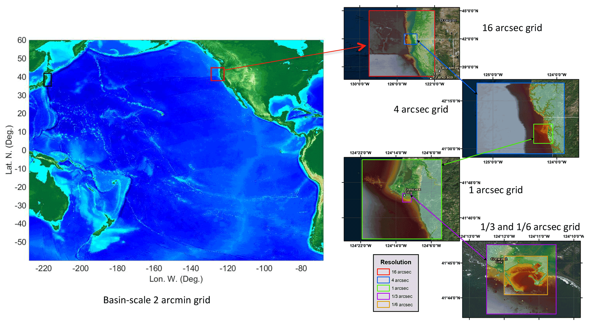
Figure 1The nested grids in the simulation of the 2011 Tohoku-Oki tsunami impact on Crescent City harbor, Crescent City, California (Tehranirad et al., 2021). The nesting process scales down the grid resolution from 2 arcmin in the ocean basin domain to arcsec in the harbor domain. The same simulation was conducted using the present model nesting framework in Sect. 4.4. Courtesy of Google Maps © 2021 Google, © TerraMetrics.
Yamazaki et al. (2011) implemented a two-way nesting method in their dispersive depth-integrated, non-hydrostatic wave model for tsunami applications. The nesting model framework was based on a block-structured scheme with multiple prescribed nested grids. They used this model to simulate the 2009 Samoa tsunami and the coastal inundation caused in the Pago Pago harbor and reported good efficiency and accuracy of the two-way nesting model framework. However, it is not clear whether this two-way nesting scheme was parallelized and how the mega-data structure was handled in the nesting framework. Recently, Chakrabarti et al. (2017) implemented the fully nonlinear and dispersive Boussinesq model FUNWAVE-TVD in the block-structured AMR framework Cactus, which has been widely used in the field of astrophysics (Löffler et al., 2014). They showed that shallow-water waves could be simulated at higher resolution, with a reasonable computational cost, which also allowed using an improved higher-order representation of the vegetation drag force. However, in this application, the nested grids were statically prescribed to reduce the computational cost from using dynamically adapted grids with a Boussinesq-type model. In addition, the Cactus-based version of FUNWAVE-TVD relies on a specific library package and configuration (Oler et al., 2016), limiting its general applications in the large user community.
There are significant challenges implementing an AMR and two-way multi-grid-nesting framework in a parallel computing environment. Load balance, communication between parent and child grids, and mega-data management are major issues in MPI-based (message passing interface) programs. Load balance is important for CPU (central processing unit) scaling, in terms of synchronization of solutions across refinement levels. Dubey et al. (2014) reviewed load balancing methods in several public-domain AMR packages and pointed out the difficulties in achieving workload balance in the AMR framework. In a parallel multi-level grid system, the parent–child grid communication is also critical to modeling efficiency. Strategies to build direct communication between multi-level grids cross-ranks can be found in many AMR packages (Dubey et al., 2014). A multi-level grid system makes the mega-data management more complex, especially for tree-structured data. Finally, it is important to optimize the amount of mega-data replication according to both the communication cost and memory cost (Dubey et al., 2014).
The limitation of the prior Cactus implementation of an AMR version of FUNWAVE-TVD to a specific high-performance computing (HPC) platform (Chakrabarti et al., 2017) motivates the development of a more platform-independent implementation of a two-way nesting scheme. The primary objective for the present development is to provide a generic interface which can be used with any HPC platforms. The interface is used as a master program to manage model input/output, the time sequencing, and two-way nesting processes between grids at two different levels. Data exchanges between parent and child grids are performed using the linear interpolator and restriction operator. We used an equal-load scheme in workload balance and applied a strategy of shared array allocation for data management. The interface is developed separately from the core program and does not interfere with the main solver of FUNWAVE-TVD. Hence, the package of the combined interface and core program can be updated concurrently.
In the following, a brief description of the FUNWAVE-TVD model is given in Sect. 2. Section 3 describes the two-way nesting interface, including the general algorithm, workload balance, and flowchart of a master program. Applications are presented in Sect. 4. Section 5 provides a summary of the present study.
2.1 The TVD version of the fully nonlinear Boussinesq model
The scope of the present work is to develop a multi-grid-nesting framework for the Boussinesq-type wave model FUNWAVE-TVD, a widely used public-domain model in the nearshore and tsunami research community. FUNWAVE was initially developed by Kirby et al. (1998) based on the fully nonlinear Boussinesq equations derived by Wei et al. (1995). The development of the Total Variation Diminishing (TVD) version of the model was motivated by a growing demand for phase-resolving modeling of nearshore waves and coastal inundation during storm or tsunami events. The conservative form of the Boussinesq equations was discretized by a hybrid method combining finite-volume and finite-difference TVD-type schemes. The model was developed in both the Cartesian coordinates (Cartesian mode; Shi et al., 2012) and spherical coordinates (spherical mode; Kirby et al., 2013). The Cartesian mode solves the fully nonlinear Boussinesq equations, initially derived by Wei et al. (1995), with the second-order correction of vertical vorticity by Chen (2006) and the moving reference level of Kennedy et al. (2001). The spherical mode solves the weakly nonlinear, weakly dispersive Boussinesq equations in spherical coordinates (Kirby et al., 2013). The code was parallelized using the domain decomposition method based on MPI for CPU-based high-performance computing (HPC) clusters, and the GPU-accelerated (graphics processing unit) program is for single- and multi-GPU systems (Yuan et al., 2020). In tsunami applications, where nearshore waves are expected to be strongly nonlinear, a combination of deep-water spherical and nearshore Cartesian grids has often been used in the one-way coupling nested-grid framework (e.g., Grilli et al., 2013, 2015, 2017; Schambach et al., 2019, 2020; Tappin et al., 2014).
2.2 Governing equations in the Cartesian and spherical coordinate systems
Although the sets of equations in Cartesian and spherical coordinate systems are different, the two FUNWAVE modes were developed within the same numerical framework and using the same TVD-type solver. The combined form of the Boussinesq equations in the two coordinate systems can be written as
where Ψ and Θ(Ψ) are the vector of conserved variables and the flux vector function, respectively, given by
where (P,Q) are the horizontal volume fluxes of
where with h being the water depth and η being the surface elevation; uα is the horizontal velocity vector at a reference depth zα; and is the depth-averaged second-order horizontal velocity of O(μ2), in which μ is ratio of characteristic water depth to a horizontal length, a dimensionless parameter quantifying the magnitude of wave dispersion. The velocity components (U,V) combine uα and the dispersive terms V1:
The velocity uα is obtained by solving a system of equations with a tridiagonal matrix formed by Eq. (4).
In Eq. (2), Sp is the spherical coordinate correction factor defined for the spherical mode as
in which θ and θ0 are the latitude and the reference latitude, respectively (see Kirby et al., 2013). For the Cartesian mode, Sp=1. The last term S in Eq. (1) contains the Boussinesq source terms, which are detailed in Shi et al. (2012) for the Cartesian mode and Kirby et al. (2013) for the spherical mode.
2.3 Numerical schemes
In FUNWAVE-TVD, the HLL (Harten–Lax–van Leer) Riemann solver with several options of finite-volume schemes in different orders of accuracy was implemented. By default, the fourth-order accurate MUSCL-TVD scheme (monotonic upstream-centered scheme for conservation laws; Erduran et al., 2005) was applied for discretizing the leading-order spatial derivative terms of the equations, while the dispersive terms were discretized by a second-order centered finite difference scheme. Choi et al. (2018) compared the performance of the MUSCL-TVD, WENO (weighted essentially non-oscillatory), and MLP (multi-dimensional limiting process) schemes in FUNWAVE-TVD and showed that the MUSCL-TVD scheme with a van Leer limiter provides an accurate and stable solution in long-term simulations. Here, we only briefly present the basic methods related to the nesting procedure in the present work. Readers interested in detailed numerical schemes are referred to Shi et al. (2012) and Choi et al. (2018).
For a time-stepping scheme, FUNWAVE-TVD uses the third-order strong stability-preserving (SSP) Runge–Kutta scheme (Gottlieb et al., 2001), with an adaptive time stepping based on the Courant–Friedrichs–Lewy (CFL) condition prescribed as
where Ccfl is the Courant number and Δx and Δy are grid sizes in the x and y directions, respectively.
Although the conservative equations of Eq. (1) are solved explicitly using the HLL Riemann solver, a system of tridiagonal matrix equations derived from Eq. (3) needs to be solved to get the velocity at the reference level, which is done with Thomas' algorithm (Naik et al., 1993).
Various boundary conditions were implemented in the model, including a wall boundary condition, wave periodic boundary condition, wavemaker boundary condition, and absorbing or partially absorbing boundary conditions. The wall boundary condition is the main boundary condition, dealing with either full wave reflection or a moving shoreline. Ghost cells are used in the grid to implement a mirror boundary condition. As mentioned earlier, the multi-grid interface is developed separately from the core program, and each grid in the nesting system runs the same core program for given initial and boundary conditions.
2.4 Parallelization
The CPU code uses a domain decomposition technique to subdivide the problem into multiple regions and assign each subdomain to a separate processor core. Each subdomain region contains an overlapping area of ghost cells, which is three rows deep, as required by the fourth-order MUSCL-TVD scheme. MPI with non-blocking communication is used to exchange data in the overlapping region between neighboring processors. The tridiagonal matrices are solved using the parallel pipelining tridiagonal solver described in Naik et al. (1993).
Data exchanges between neighboring subdomains are conducted through the ghost cells at every Runge–Kutta time step. To increase the model efficiency, the values of dispersive terms, in addition to the major variables (), are also exchanged at the ghost cell boundaries.
3.1 Algorithm
For simplicity, we consider first a two-level nested-grid system containing the parent grid Ω0 and the child grid Ω1 as shown in Fig. 2. The parent grid has a larger grid size Δx0, while the child grid has a smaller grid size Δx1. The grid refinement ratio is thus defined as . The boundary of the child grid is denoted by Γ, which has ghost cells. Following the general procedure for two-way nesting, such as detailed in Debreu and Blayo (2008), the partial differential equation of Eq. (1) can be rewritten as
where represents a general operator. The equation is discretized in Ω0 and Ω1 grids by
respectively, where L0 and L1 denote the discretized form of the same operator L at a different resolution. In the two-way nesting framework, the child grid solution is driven by the lateral boundary conditions along Γ, while the parent grid is updated using the child grid solution. Noting that both of the procedures need interpolation/mapping processes, we define the interpolators Is and It and the restriction operator R. Is and It perform interpolations in space and time, respectively, at Γ, and R performs the mapping from the child grid solution to the parent grid solution. Assuming the grid refinement factor s equals the time refinement factor based on the CFL condition of Eq. (6), the two-way nesting can be described by the following pseudo code:
Four ghost cells are used along Γ. Here, we want to mention that the number of ghost cells in the MPI-based parallelization is three, as required by the higher-order numerical schemes used in the model. The nesting scheme needs one more cell for the requirement because of recalculating rather than passing values of the ghost cells.
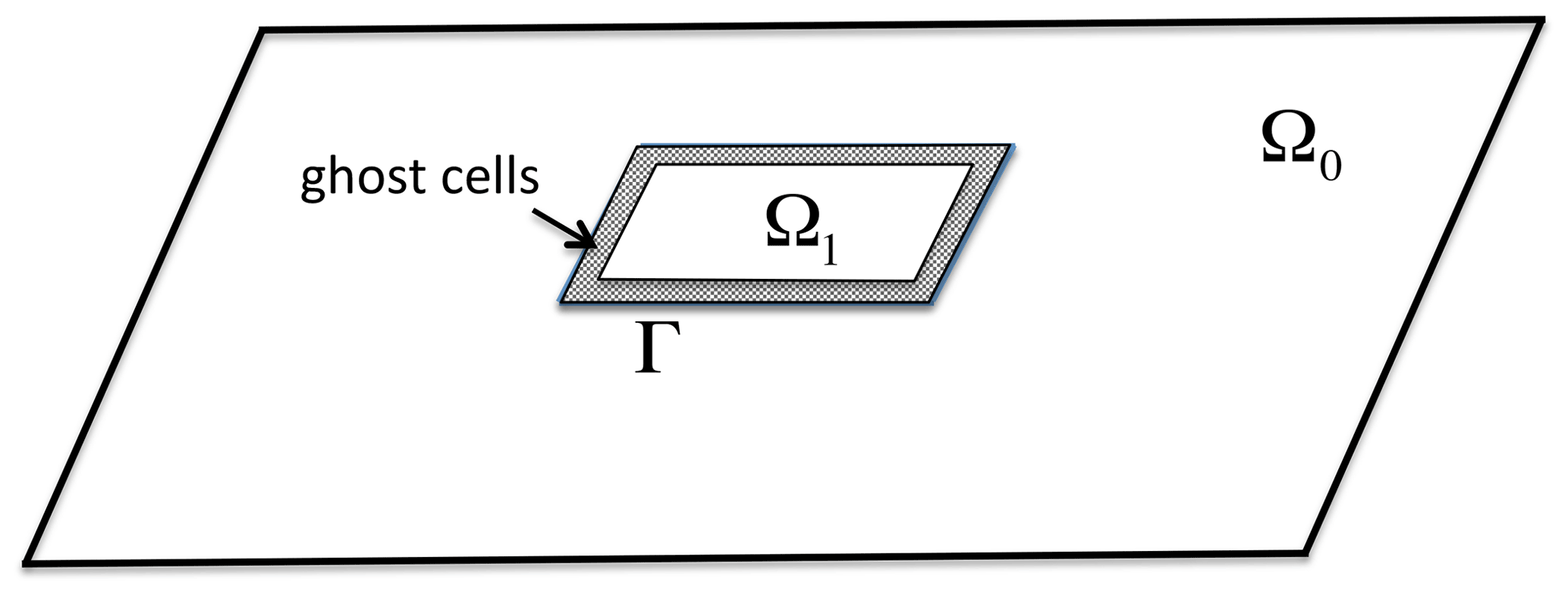
Figure 2Schematic drawing for the two-way nesting method. The parent grid Ω0 has a coarse-resolution grid, while the child grid Ω1 is high resolution. Ghost cells (four rows) are specified along the inter-grid boundary, Γ.
Based on the assumption that the grid refinement factor equals the time refinement factor and that the linear relation between the time step and grid spacing holds in the CFL criterion, the child time step between two parent time levels is constant and can be written as
where Δtparent and Δtchild denote the parent time step and child time step, respectively. In addition, the tridiagonal solver required to solve Eq. (4) in each child grid is performed for given nesting boundary conditions at ghost cells.
3.2 Interpolator and restriction operator
In some two-way nesting methods used in 3D ocean models, the interpolator Is and It and the restriction operator R are complex due to issues raised by mass/momentum imbalance, barotropic/baroclinic mode splitting, and the staggered grid configuration (Debreu et al., 2012). To ensure mass and momentum conservation during the two-way nesting, a correction may be needed at the nesting boundaries according to specific numerical schemes. This especially occurs in a nesting scheme using discretizations of the nonconservative forms of mass and momentum equations, based on finite differences, because the flux of mass or momentum is expressed by a nonlinear term. Hence, typically, the mass flux (h+η)u is no longer conserved when performing a linear interpolation individually for η and u at a nesting boundary.
FUNWAVE-TVD is based on the conservative forms of mass and momentum equations, in which advection is performed using the finite-volume method (Shi et al., 2012). The latter makes it possible to use a linear or doubly linear interpolator in the nesting method, without changing the conservative property of the equations. In the AMR application of an NSWE model, Liang (2012) demonstrated the conservative property of the linear operator used in the finite-volume Godunov-type scheme and, later, pointed out that the operator preserves both mass conservation and the C property (i.e., conservation property) as the wetting–drying process involved in the grid nesting. FUNWAVE-TVD uses a finite-volume scheme similar to Liang (2012) and Liang et al. (2015), and, therefore, its conservative property should be maintained when applying a linear operator. Unlike Liang (2012), who used a second-order scheme, FUNWAVE-TVD applies a higher-order Godunov-type scheme; hence ghost cells must be used along nesting boundaries.
Consequently, a doubly linear interpolation is applied to ghost points in the child domain, using values from the parent grid. Thus, at a ghost point (X,Y) in the child domain, which is surrounded by four points, (xij,yij), , , , in the parent domain, a given variable φ1 is interpolated as
where,
where φij, , , are values of the variable in the parent domain.
The restriction operator uses linear averaging, which guarantees the conservation of mass and momentum. The restriction operator can be expressed as
where φ2 represents the averaged value passing to the parent grid, is the value at (i,j) in the child grid, and (M,N) represents the numbers of child grid cells in (x,y) directions embedded in each parent grid cell.
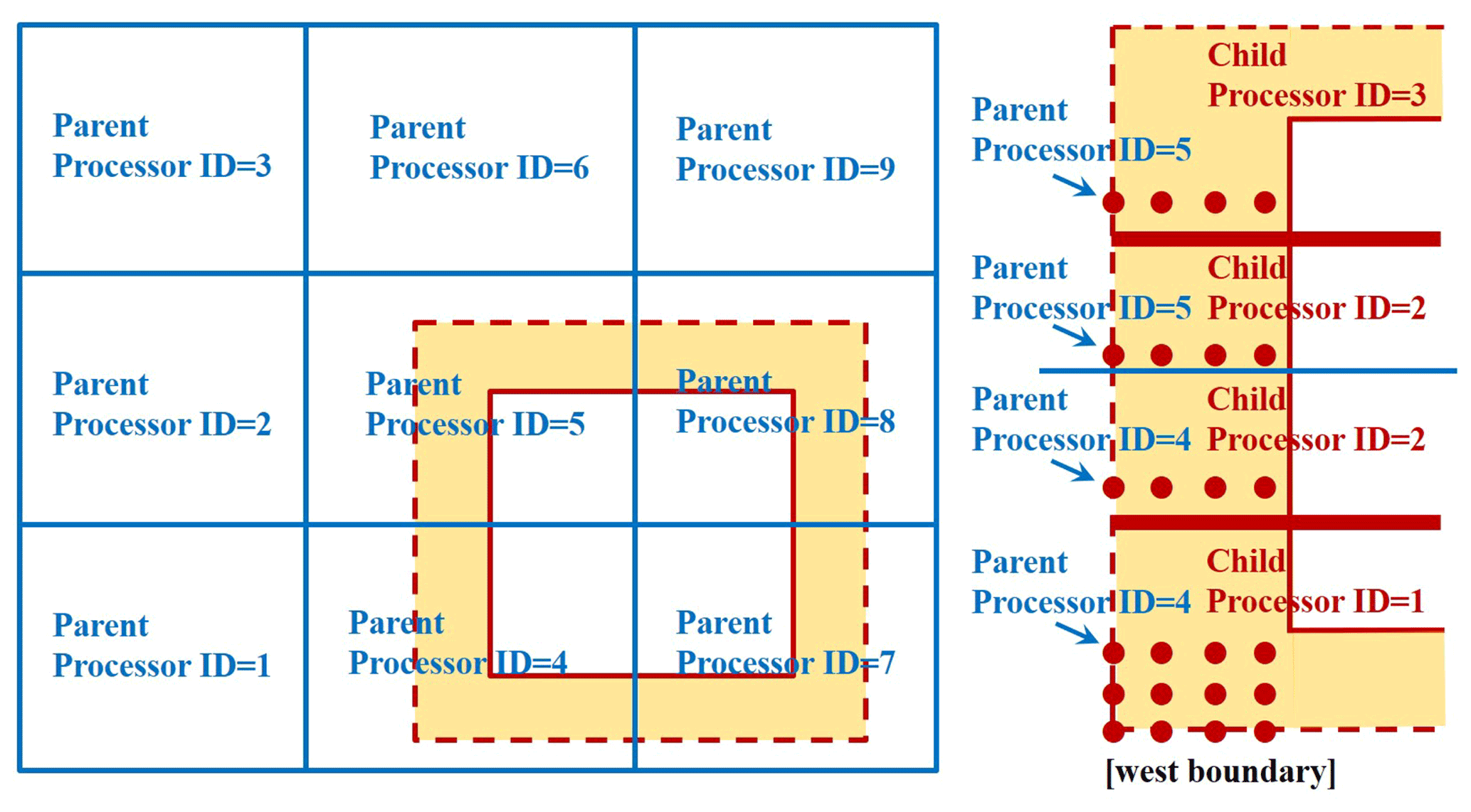
Figure 3Decomposed domain by MPI and the relation between the parent processor ID and child processor ID.
Both the interpolator and the restriction operator are performed to and V, which pass the values back and forth between the child domain Ω1 and the parent domain Ω0 in the two-way nesting process. It should be pointed out that U and V are not necessarily included in the interpolation/restriction processes because they can be calculated based on η,uα, and vα. However, our tests show that directly using the passed U and V can make the model more efficient and does not affect the results much.
3.3 Workload balance and data management
The MPI parallelization of FUNWAVE-TVD uses a 2D Cartesian topology for the domain decomposition, which subdivides the computational domain into a 2D grid, each cell of which is assigned to a processor. The size of the global arrays is not necessarily divisible by the number of processors, but an evenly divisible configuration results in a perfectly equal workload. To ensure workload balance in computations involving multi-grid levels, we used the same domain decomposition algorithm on all grid levels with the same number of processors. This algorithm is especially efficient for block-structured or patch-structured nesting schemes, as described in Debreu et al. (2012).
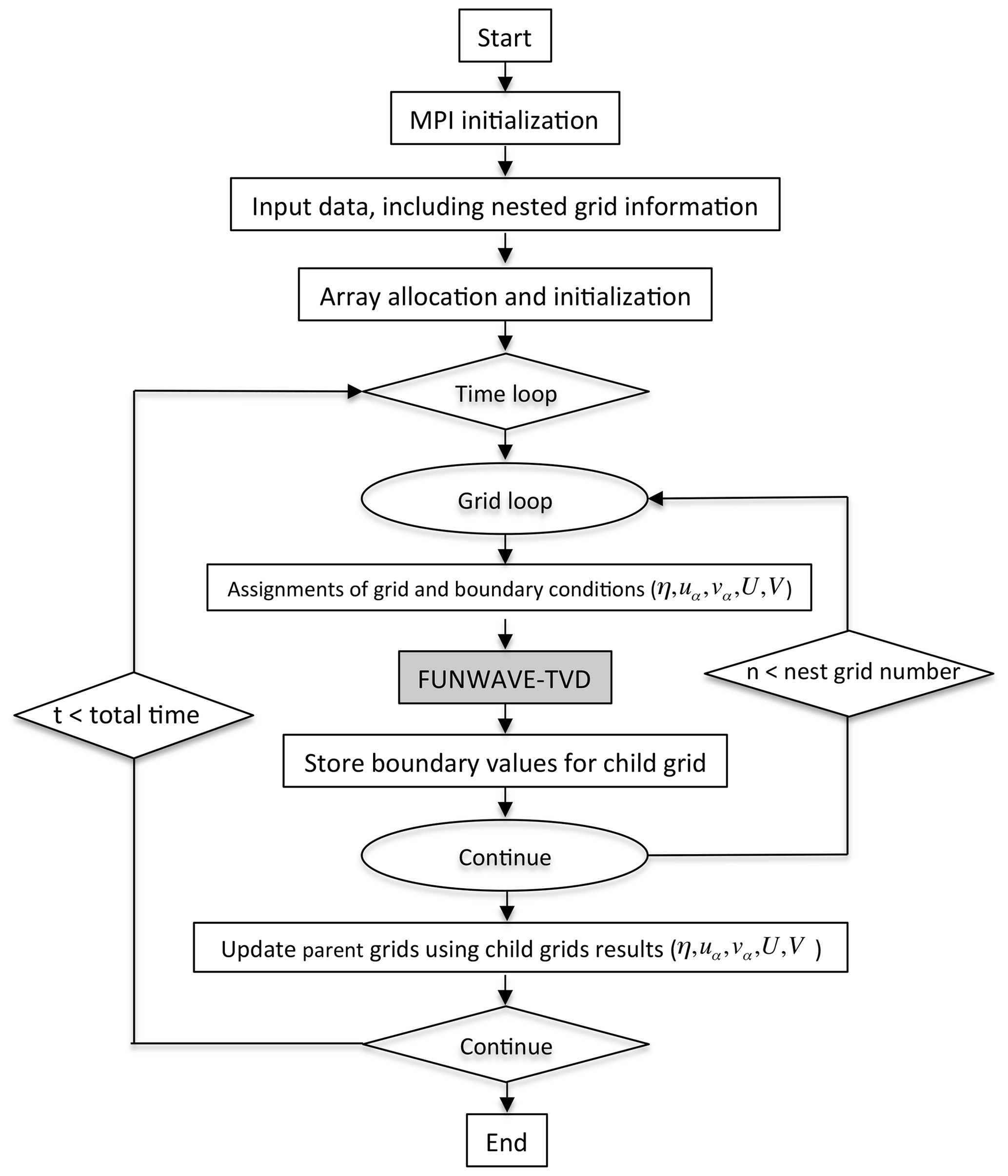
Figure 4Flowchart of the two-way nesting interface. t and n represent time and grid level, respectively.
Figure 3 gives an example of the domain decomposition and communication at two-grid levels in a system of nine processors. Both the parent domain and the child domain are decomposed evenly into a 3 × 3 grid, according to the standard 2D Cartesian virtual topology used in the MPI library, with ranks named ID . For efficient communication between the parent and child grids in the MPI-based parallel-communication system, parent–child spatial proximity is created at the beginning of the model run. The parent–child proximity is associated with the parent processor IDs and the child processor IDs at the nesting boundaries in the image distribution, as shown in Fig. 3. The parent–child proximity records the spatial relation of processor IDs between the parent and child grids and is saved in a parameter array. Therefore, the communication between the parent and child grids can be carried out straightforwardly using MPI_SEND and MPI_IRECV (MPI library) with the existing parameter array whenever a communication is needed. In this example, along the west boundary of the child grid, the child processors with ID =1, 2, and 3 communicate directly with parent processors with ID =4 and 5. In particular, the variables in the ghost cells located in child processor ID =1 are evaluated by the interpolator in the parent processor ID =4 and so on.

Figure 5Wave generation from an initial 1 m elevation still-water hump. The parent grid, Grid 1, covers the entire domain, and solid and dashed lines mark the boundaries of Grid 2 and Grid 3, respectively. Bullets mark locations of numerical wave gauges for comparing free-surface elevations.
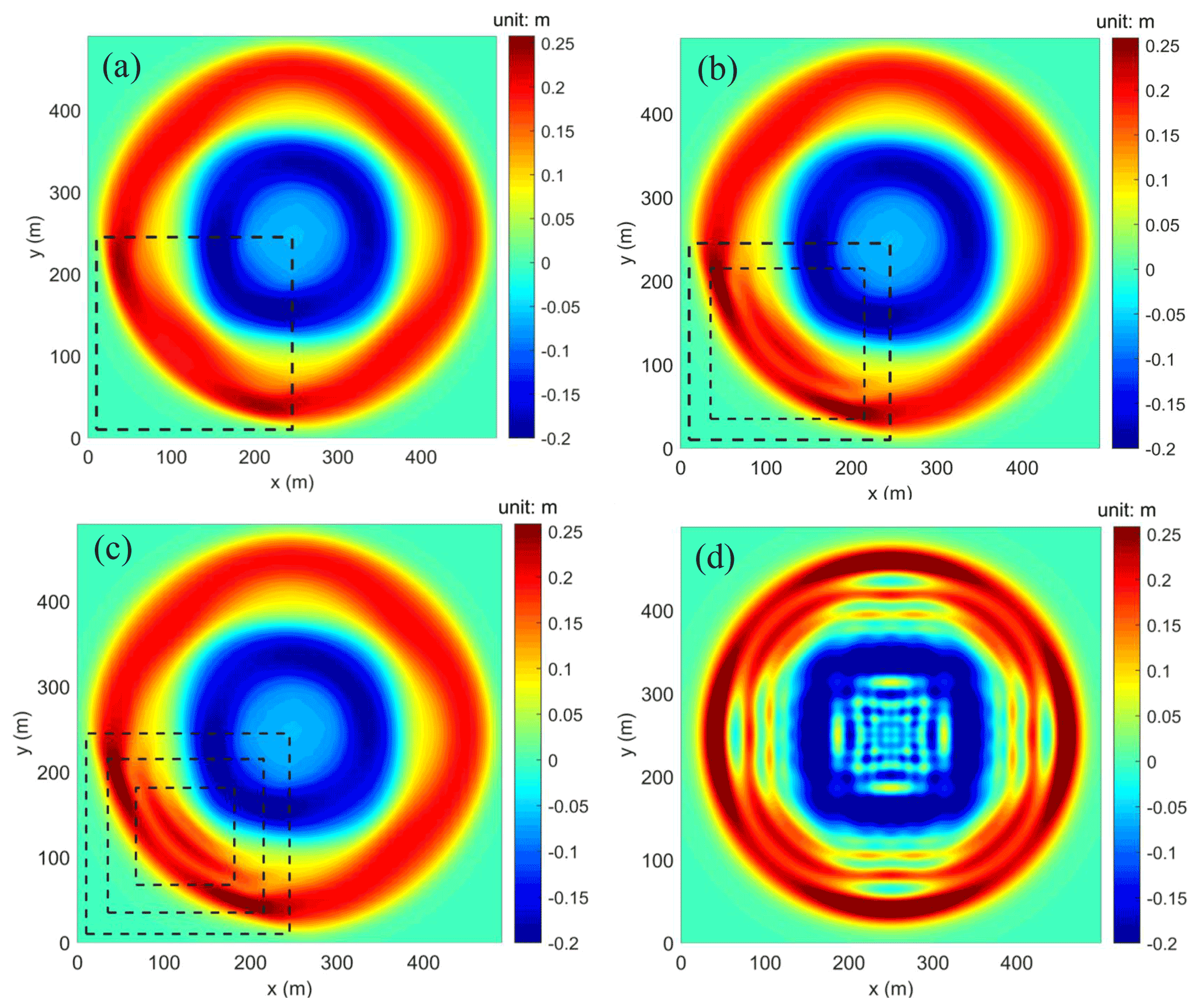
Figure 6Wave generation from an initial 1 m elevation still-water hump. Snapshots of surface elevations computed at t=23 s in (a) two-level grids, (b) three-level grids, and (c) four-level grids, with a discretization of 10, 5, 2.5, and 1.25 m, respectively (s=2), and (d) a single-level grid with a resolution of 1.25 m. Dashed lines denote the boundary of child grids.
As mentioned in the Introduction, our goal in development is to make a generic grid-nesting interface without altering the main FUNWAVE-TVD code. To achieve this, we treated the main program of the original model as a kernel, which performs computations at all grid levels. The kernel is called from the master program, which manages the time sequencing and nesting processes. A strategy of shared array allocation is used, whereby the arrays are allocated with the maximum dimension of all grids at the initialization stage, and grids at all levels share the same memory allocations. For example, in the case presented later in Sect. 4.1, the nesting system has four grid levels, the dimensions of which are (48, 48), (73, 73), (92, 92), and (91, 91) for Grids 1–4, respectively. A 2D array for η will be allocated in η(92,92), the maximum dimension among the four grids. The four grids share the same array of η(92,92), while the grids with a dimension smaller than (92,92) only use part of the allocation, i.e., (48,48) for Grid 1, (73,73) for Grid 2, and (91, 91) for Grid 4. There is no additional array allocation needed for a specific child grid with such a shared allocation strategy. It can apparently save a significant amount of computer memory and does not create an extra burden for a large number of nested grids.

Figure 7The detailed comparison between two-level, three-level, and four-level grids and single higher-resolution grid configurations along the transect crossing (0,0)–(250,250) m.
Additional storage arrays are created to store the nesting boundary conditions at different grid levels. There is no additional data structure implemented in the mega-data management.
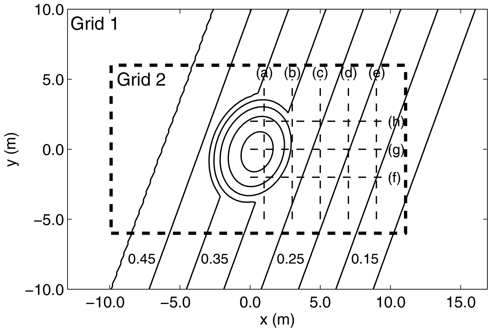
Figure 8Computational domain and bottom topography of Berkhoff et al. (1982) experiments of wave transformations over a tilted elliptical shoal on a sloping bottom. The bold dashed line box marks the area of the nested grid, Grid 2. Dashed lines (a)–(h) are transects for model–data comparisons.
3.4 Flowchart
Figure 4 summarizes the flowchart of the master program. After the MPI initialization, the program reads input data, including model parameters needed in the original model and nested-grid information. As mentioned earlier, array allocation and initialization are performed based on the maximum dimension of all grid levels. Additional arrays for the storage of boundary conditions are also allocated at this stage. Then the program starts the main time loop based on time stepping of the background (first-level parent) grid. The calculations at each grid level are conducted hierarchically inside the main time loop, with a time step based on Eq. (9). At each grid level, the model is assigned by the initial condition (solution at the last time level) and boundary conditions obtained from the Is and It interpolation processes. Then the core FUNWAVE-TVD program is called at the grid level and stores boundary values for the child grid. All parent grids are updated based on the child grid results through the R process after all subgrid levels computations are completed.
In summary, the hierarchical-type grid refinement processes are sequential, and the synchronization is conducted at each grid level. Therefore, there is no additional optimization for MPI partitions needed for the nesting framework.
Hereafter we test our new two-way coupled nested-grid solution with FUNWAVE-TVD on a series of standard idealized or benchmarking applications and then on the 2011 Tohoku-Oki tsunami case study discussed earlier.

Figure 9Experimental benchmark of Fig. 8. Snapshots of free-surface elevation at t=40 s, computed in (a) the single-grid and (b) the nested-grid models.
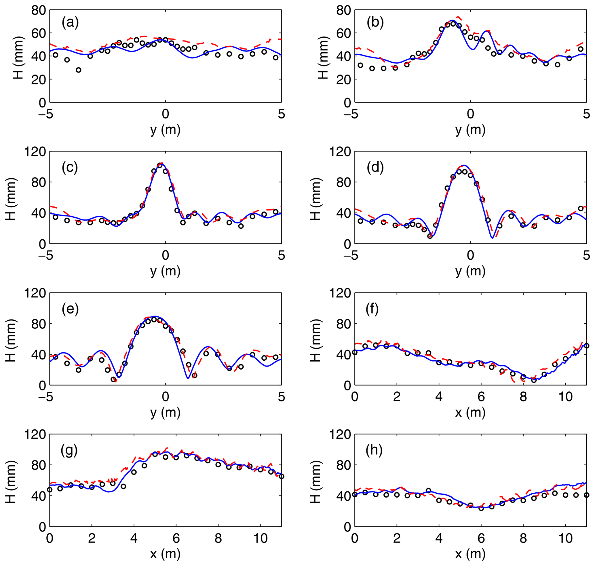
Figure 10Experimental benchmark of Fig. 8. Comparison of wave height distribution along transects (a)–(h) in (circles) experimental data and results of the (dashed) single-grid and (solid) nested-grid models.
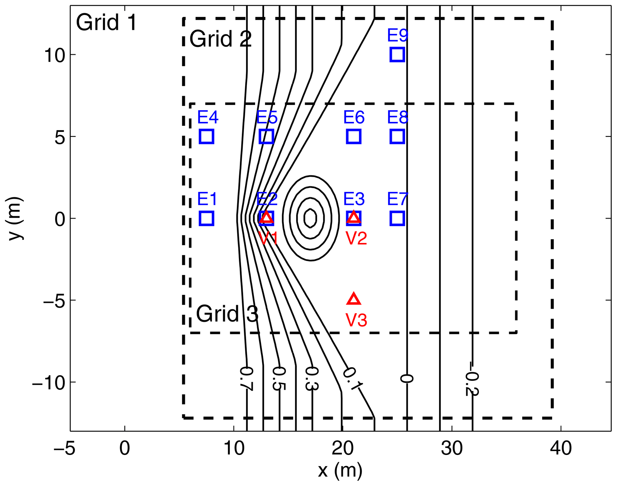
Figure 11Solitary wave runup on a shelf with an island (Lynett et al., 2010). Bathymetry contours (solid lines, in meters) and measurement locations in the computational domain. The parent grid, Grid 1, covers the entire domain; blocks with dashed lines mark the boundaries of the nested grids, Grids 2 and 3. Symbols mark locations of (□) physical/numerical wave gauges, E1–E9, and (△) velocimeters (ADVs), V1–V3.
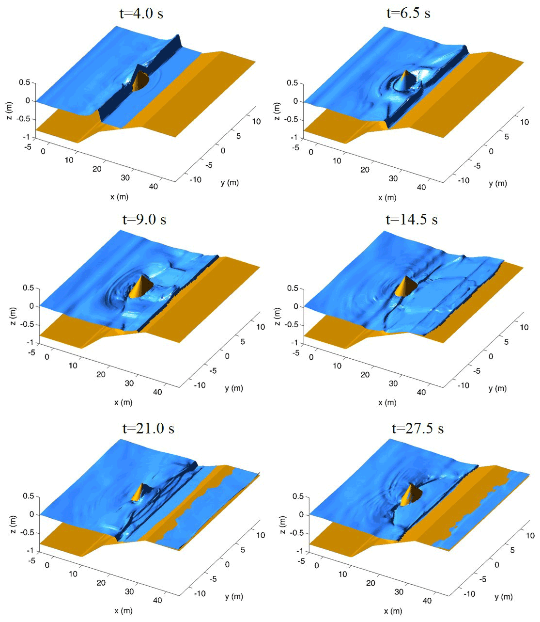
Figure 12Case of Fig. 11. Surface elevations simulated at t=4.0, 6.5, 9.0, 14.5, 21.0, and 27.5 s in a nested-grid system.

Figure 13Case of Fig. 11. Comparison of surface elevations at wave gauges in (solid) experiments and (blue and red dashed, respectively) results of the present nested and original FUNWAVE-TVD models.
4.1 Evolution of an initial rectangular-shaped hump
The evolution of waves generated from an initial arbitrary rectangular-shaped hump on the free surface is used to test the consistency of the multi-grid-nesting system and effects of the higher resolution resulting from the grid refinement. As shown in Fig. 5, a 100 m × 100 m hump with an elevation of 1 m is specified, with no initial velocity, at the center of a 500 m × 500 m rectangular domain with a 5 m water depth. Wall boundary conditions (fully reflective) are specified at the four boundaries of the domain. The initial still-water level can thus be defined as
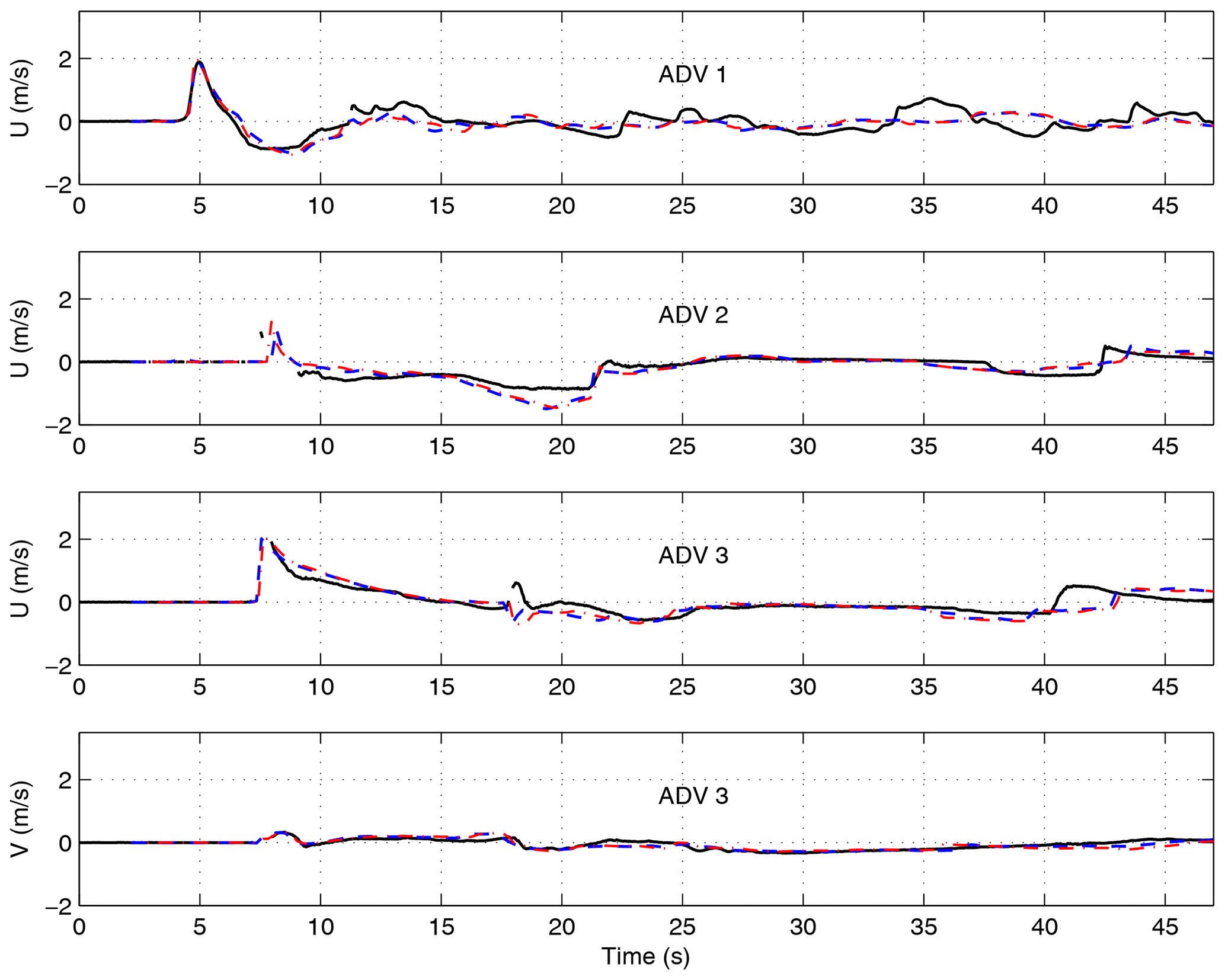
Figure 14Case of Fig. 11. Comparison of velocities at ADV locations in (solid) experiments and (blue and red dashed, respectively) results of the present nested and original FUNWAVE-TVD models.
The consistency and accuracy of the two-way nested-grid algorithm is first assessed by defining a three-level nested-grid system with identical grid resolution m in Cartesian coordinates, hence a grid refinement ratio of s=1. Grid 1 is the background parent grid, and Grids 2 and 3 are nested grids located in 10.0 m 247.5 m and 30.0 m 207.5 m, respectively. Because the refinement ratio is 1, the same numerical solution is expected whether nesting is used or not. To verify this, surface elevation time series were computed at four numerical wave gauges located at , (375,125), (125,375), and (375,375) m (see Fig. 5). The bottom-left gauge is located within the two nested grids, and its time series computed in Grid 3 is compared to those at the three gauges located in Grid 1. Because of the symmetry of the initial solution, results at the four gauges should be identical, which was verified by the comparison (not shown here), hence assessing the consistency of the nested-grid model.
Next, we examine the effects of grid refinement in a hierarchical nested-grid system for the same application. Here, the Grid 1 resolution is m, and Grid 2 and Grid 3 are nested within Grid 1, as before, but with grid resolutions of 5 and 2.5 m, respectively. Grid 2 is located in 10.0 m 245 m, and Grid 3 is in 35.0 m 215 m. An additional grid, Grid 4, was added within Grid 3, located in 67.5 m 181.25 m with a grid resolution of 1.25 m. The dimensions for Grids 1–4 are (48, 48), (73, 73), (92, 92), and (91, 91), respectively. Note that this is the example we mentioned earlier in the last section to explain the strategy of the shared array allocation. Three computations were performed using two- to four-level nested grids. Additionally, we carried out a test using a single grid with the highest resolution (1.25 m) for a comparison as suggested by one of the reviewers. Figure 6 shows a comparison of surface elevation computed at t=23 s between two- to four-level nested grids and the single grid. Because wave dispersive effects are related to grid resolution, the solution in a finer grid is not exactly the same as in a coarser grid, resulting in asymmetric distributions of surface elevations in the figure. With a two-level nested-grid system (Grids 1 and 2), Fig. 6a shows the appearance of sharper crests (dark red) in Grid 2, as compared to the solution in Grid 1. As more levels of nested grids are used, Fig. 6b and c show that shorter waves increasingly appear in the finer grids, consistent with the result from the single fine grid. Figure 7 provides the detailed comparison between the four grid configurations along the transect crossing (0,0)–(250,250) m. Short waves induced by the dispersion effect appear to be more and more apparent as nesting levels increase, closer to the result from the single fine grid.
4.2 Wave refraction–diffraction over a shoal on a sloping bottom topography
Although the main targeted applications of our new two-way grid-nesting model system are tsunami simulations in multi-scale cases, the method can also be applied to the modeling of ocean wave transformations in coastal areas. This is demonstrated here by simulating the laboratory experiments of Berkhoff et al. (1982), for wave refraction–diffraction over a shoal on a sloping bottom topography, both rotated by 20∘ off the y axis (Fig. 8). This experimental dataset has served as a standard benchmark for assessing the accuracy and performances of numerical wave models for simulating wave shoaling, refraction, diffraction, and nonlinear dispersion. Shi et al. (2011) showed that the original version of FUNWAVE-TVD accurately reproduces measured wave heights in this experiment.
Two numerical simulations were carried out for (i) the original single-grid model and (ii) a two-level nested-grid model (Fig. 8). Both models are set up in a rectangular domain with Cartesian coordinates, −13 m 16.9 m and −10 m 10 m. The single-grid model has grid resolutions of Δx=0.025 m and Δy=0.05 m. In the two-level grid model, Grid 1 is coarser with Δx=0.1 m and Δy=0.2 m resolutions, and the finer Grid 2 is nested in the region of −9.9 m 11.075 m and −6 m 6 m, with a resolution of Δx=0.025 m and Δy=0.05 m identical to those of the single-grid model, corresponding to a grid refinement ratio of thus s=4. The total numbers of cells in Grid 1 and 2 are 30 300 and 202 440, respectively, which is much smaller than the 480 000 cells of the single-grid model.
In both model setups, regular waves with a period T=1 s and an amplitude A=4.64 cm are generated, as in experiments, by a wavemaker located at m. Sponge layers with a width of 2 m were specified on the left and right boundaries of both the single-grid domain and Grid 1 in the nested-grid model.
Figure 9 shows snapshots of surface elevation computed at t=40 s in both model setups. Compared to the single-grid model, which uses the finest grid resolution over the entire domain, the nested-grid model, which only uses it in Grid 2, shows that waves are numerically damped due to the coarse-grid resolution used outside of Grid 2. Over the shoal and slope behind it, results in both the nested Grid 2 and the single grid show similarly intense wave shoaling, refraction, and diffraction patterns. However, in the nested-grid model, additional spurious wave diffraction effects can be seen around the lateral nesting boundaries due to the wave damping on the coarse-grid side.
Figure 10 shows comparisons of both model results with experimental data for the wave height variation along the transects marked in Fig. 8. For all transects, both the single-grid and nested-grid model results agree well with the data. As expected from the spurious diffraction effects, compared to the single-grid model, the nested-grid model predicts slightly smaller wave heights at the ends of transects (a)–(e).
Regarding computational efficiency, in this application, the cost of the nested-grid model is about 46.5 % of the single-grid model. It should be mentioned that this test is only for verification of the nested-grid algorithm and is not a typical case for demonstrating the efficiency of the nested-grid method.
4.3 Solitary wave runup on a shelf with an island
A second experimental benchmark, for the runup of a solitary wave over a complex nearshore bathymetry with an island (Fig. 11), is simulated to assess the accuracy of the wetting and drying algorithm along the model shoreline, in a nested-grid system. These experiments were performed in the large wave basin of Oregon State University's O.H. Hinsdale Wave Research Laboratory (Lynett et al., 2010). The 3D bathymetry was constructed in the 48.8 m long and 26.5 m wide basin, with a 2.1 m depth. It consists of a plane slope connected to a triangular shelf with a conical island over the shelf (Figs. 11 and 12). Surface elevations were measured at nine locations using wave gauges (E1–E9 in Fig. 11), and velocities were measured at three locations by acoustic Doppler velocimeters (ADVs) (V1–V3 in Fig. 11). Details of the experiment can be found in Lynett et al. (2010). Shi et al. (2012) applied the original version of FUNWAVE-TVD to this case.
In the model simulations, a three-level nested-grid system is set up with Grid 1, Grid 2, and Grid 3 shown in Fig. 11. The model setup for Grid 1 is similar to Shi et al. (2012), except that the grid resolution is coarser, with m, versus 0.1 m in the original model. The nested grids, Grid 2 and Grid 3, have 0.2 and 0.1 m resolution, respectively (hence, s=2), and are centered in the middle of the domain where wetting and drying frequently occur due to the moving shoreline during runup. As measured in experiments, an incident solitary wave of height Ho=0.39 m is specified in Grid 1, in the constant depth ho=0.78 m region on the left side of the model, at −5 m 5 m, with its crest initially located at x=0. The initial solitary wave condition is based on Nwogu's extended Boussinesq equations (Wei and Kirby, 1998). With this represents a strongly nonlinear incident wave. A summary of the nested-grid configuration is given in Table 1.
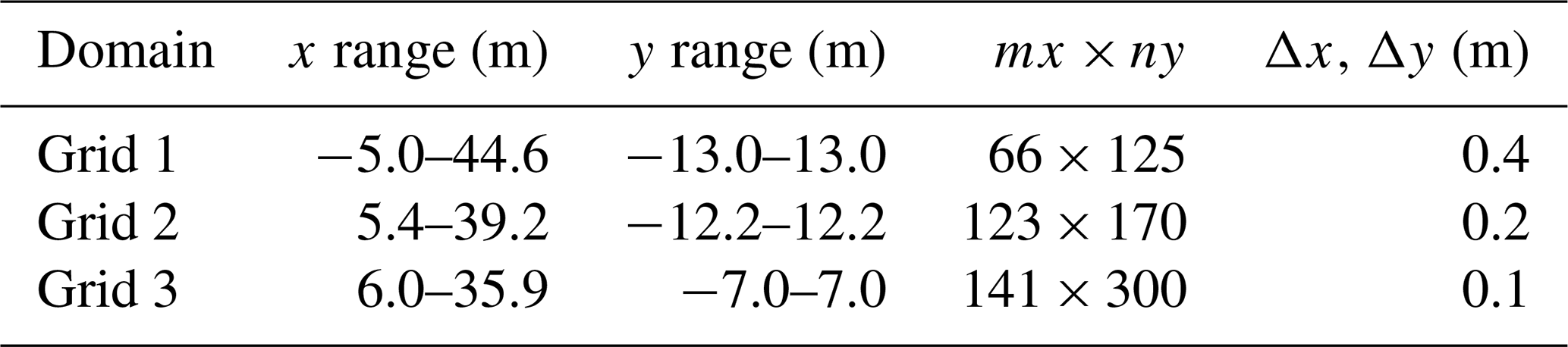
Table 2Grid parameters for the 2011 Tohoku-Oki tsunami simulation.

Figure 12 shows snapshots of surface elevations simulated in the nested-grid model, constructed using results from all grids, wherever the highest-resolution results are available. Results show successively that wave breaking occurs at t=4.0 s; that edge waves collide behind the island at t=6.5 s; and that a breaking bore forms at t=9.0 s, with its front running up and down the upper slope and beach terrace, from t=9.0 to 27.5 s. These are all quite complex processes that appear well-resolved in the nested grids. Figure 13 shows the comparison of model results with experimental data for surface elevations measured at the nine wave gauges (E1–E9 in Fig. 11). Results from the single-grid model (with a grid resolution of 0.1 m) are also plotted in the figure for comparison. Surface elevations simulated in the new nested-grid model are quite close to those in the original single-grid model, and both agree well with the experimental data. Slight differences between the nested grid and single-grid models can be seen at Gauge 9, likely because this gauge is located in Grid 2, for which the resolution is lower than that in the single-grid model; all the other gauges are located in Grid 3, which has the same resolution as the original single-grid model.
Figure 14 similarly compares time series of simulated and measured mean horizontal velocity at three ADVs (V1–V3 in Fig. 11). Results from the nested-grid model are all close to those of the original single-grid model, and both agree well with the data. We note that all ADVs are located in Grid 3, which has the same grid resolution as the original single-grid model; hence results of both models are expected to be consistent.
4.4 2011 Tohoku-Oki tsunami impact on Crescent City harbor, Crescent City, California
As mentioned in the introduction, the multi-scale modeling of transoceanic tsunamis is a typical application of the nesting grid technique. Tehranirad et al. (2021) used the one-way nesting technique with six-level nested grids to simulate the impact of the 2011 Tohoku-Oki tsunami, particularly morphological changes, on the Crescent City harbor, Crescent City, California. This harbor is known for its vulnerability to tsunamis due to wave-guiding effects caused by a ridge feature in the bottom topography of the Pacific Ocean (Grilli et al., 2013). During the 2011 tsunami, the Crescent City harbor, Crescent City, California, experienced extensive damage caused by a significant inundation but by most of all strong currents induced within the harbor by successive long waves in the incoming tsunami wave train. Tsunami-induced oscillations of the harbor, as well as currents, were reported to have lasted for several days in the harbor (Wilson et al., 2012), due to nearshore edge waves associated with the tsunami event. When using that many levels of grids, the multi-scale modeling using the one-way nesting technique is particularly cumbersome, in terms of the manual post-processing it involves. Hereafter, we repeat this simulation using the new two-way nesting framework. Unlike the three earlier tests, which used the Cartesian mode, this test uses spherical coordinates.
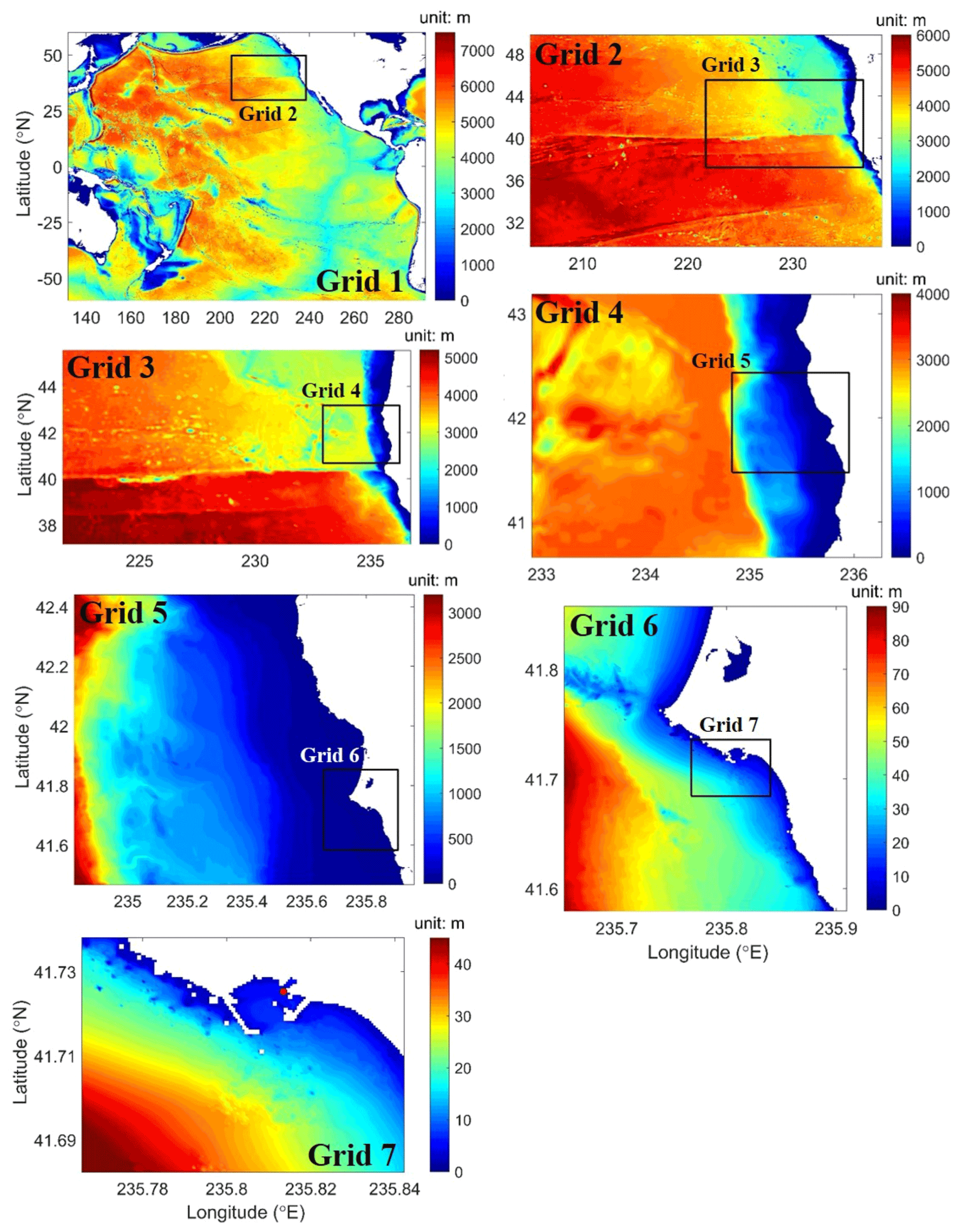
Figure 15Nested-grid simulation of the 2011 Tohoku-Oki tsunami. Bottom topography and computational domains for Grids 1 to 7. Red circles in Grid 7 denote numerical wave gauge locations.
The nested-grid system uses seven levels, with grid resolutions varying from 4 arcmin at the ocean basin scale to 1/32 arcmin around the harbor and a nesting ratio of s=2. As shown in Fig. 15, with a high resolution of arcmin in Grid 7 (or about 53 m), the model is able to resolve the harbor structures quite well. Following Tehranirad et al. (2021), the bathymetry used to define the model grids was constructed by combining 1 arcmin ETOPO1 data (Amante and Eakins, 2009), 3 arcsec Coastal Relief Model (CRM) data (NOAA National Geophysical Data Center, 2003), and the local 10 m resolution tsunami digital elevation model (DEM) of the Crescent City harbor, Crescent City, California (Grothe et al., 2011). The tsunami was generated using the same source configuration as in Grilli et al. (2013) and Kirby et al. (2013). Model parameters were specified according to Tehranirad et al. (2021). Table 2 summarizes the locations, dimensions, and grid sizes of the nested grids.
Figure 16 shows snapshots of tsunami surface elevations computed in the basin-scale Grid 1 and the nested grids, Grid 5 and Grid 7, at t=11.18 and 11.43 h, when the water surface elevation within the harbor reaches its maximum and minimum levels, respectively (Fig. 17). The model shows the generation of edge waves propagating along the coast (Grid 5), which were not simulated in Tehranirad et al. (2021) one-way nesting computations. The two-way nesting is a more relevant technique to model waves propagating across nesting boundaries, without significant wave reflection from the boundaries.
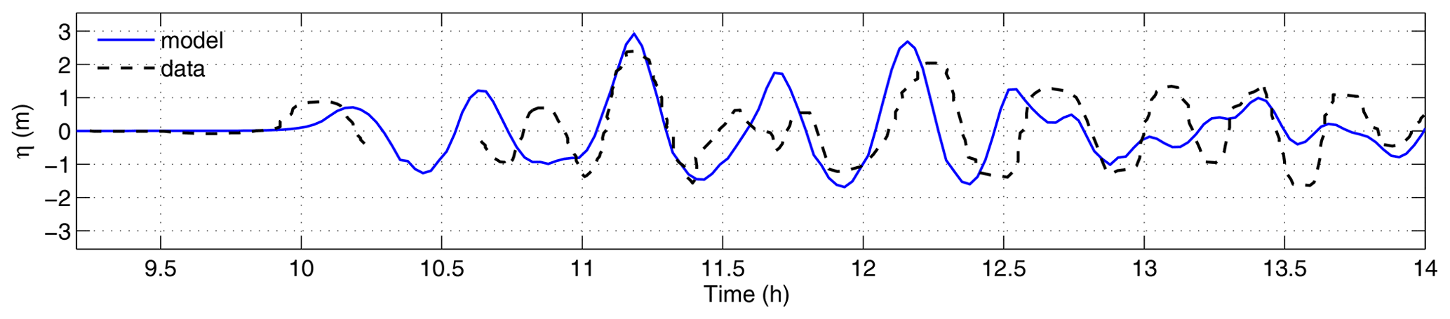
Figure 17 compares the modeled surface elevation with the data measured at the gauge location within the harbor (red circle in Grid 7 in Fig. 15). Following Tehranirad et al. (2021), the model results were shifted by 8 min backward to compensate for the time delay identified in earlier studies, which was possibly caused by compressibility and earth elasticity effects (Allgeyer and Cummins, 2014; Wang, 2015; Abdolali and Kirby, 2017; Abdolali et al., 2019). Overall, the model shows a good agreement with the data, although the largest wave crests are slightly overpredicted.
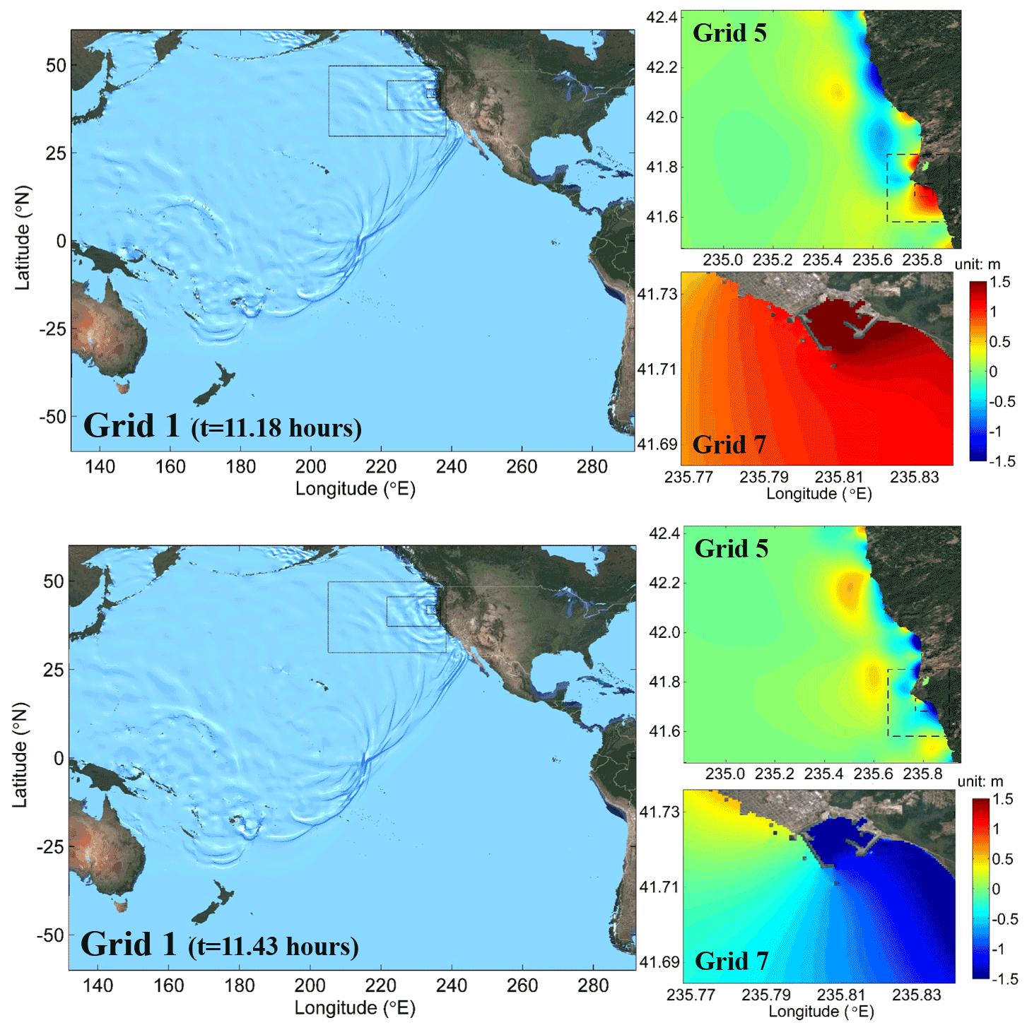
Figure 16Same case as Fig. 15. Snapshots of tsunami surface elevations simulated in Grid 1, Grid 5, and Grid 7 at t=11.18 and 11.43 h. Courtesy of Google Maps © 2021 Google, © TerraMetrics.
The main goal of this study was to develop a multi-grid-nesting interface for the Boussinesq wave model FUNWAVE-TVD which can be used as a master program to manage time sequencing and nesting processes and make it both easier and more accurate and efficient when performing multi-scale tsunami simulations. The background model couples a series of submodels with grid refinement in a hierarchical manner. Unlike other AMR-type models, the new modeling framework does not alter the original solver, and hence FUNWAVE-TVD can still be used as a standalone program for each individual grid.
The nesting algorithm performs a two-way coupling between the parent and child grids. The child grid is driven by the boundary conditions provided by the parent grid. Linear interpolators are performed both in time and space at the ghost cells of nesting boundaries. The parent grid is updated with results from the child grids using a linear restriction operator. No correction of mass and momentum is needed during the nesting process because of the use of conservative forms of mass and momentum equations.
Workload balance is handled by an equal-load scheme, which performs the same domain decomposition algorithm on all grid-levels using the same number of processors, guaranteeing equal CPU load over the entire computation. Communication between the parent and child grids is direct without a data-gathering process. The parent–child proximity is precalculated at the beginning of the model run and, hence, does not cause additional computational cost. A strategy of shared array allocations is used in data management. Grids at all levels share the same memory allocations, and no additional memory allocation is required, allowing for a large number of nesting levels to share the same memory allocation.
The nested-grid model was verified on four applications, three of which are standard benchmarks and one of which is a tsunami case study. The numerical test of wave evolution from a rectangular hump examined the consistency and general performance of the nesting algorithm. The simulation of the Berkhoff et al. (1982) experiment showed that the model is capable of simulating surface waves and their transformation in shallow water, which involves dispersive and nonlinear effects. The simulation of experiments for solitary wave runup on a shelf with an island was used to assess the accuracy of the wetting and drying processes in the nested-grid system. The last application, the simulation of the 2011 Tohoku-Oki tsunami and its effects on the Crescent City harbor, Crescent City, California, demonstrated the robustness of the two-way nesting model for the multi-scale modeling of transoceanic tsunamis and their coastal effects.
As mentioned at the beginning of the paper, a combination of the weakly nonlinear spherical mode and the fully nonlinear Cartesian mode has often been used in the one-way coupling nested-grid framework for transoceanic tsunami simulations. However, the nesting interface developed in the present study cannot be used for such mixed-mode applications. It is necessary to further develop the spherical mode based on the fully nonlinear Boussinesq equations. This development may be left for future work, noting that any new developments in the model will not interfere with the nesting interface developed here. Future work may also include the development of an interface for the GPU version of FUNWAVE-TVD and of an adaptive mesh refinement algorithm for the nesting framework.
The computer code, all examples illustrated in the paper, MATLAB post-processing scripts, and data used in this research are archived at https://doi.org/10.5281/zenodo.4735599 (Shi, 2021). The code of the multi-grid-nesting interface and the original FUNWAVE-TVD model are maintained at the GITHUB site: https://github.com/fengyanshi/FUNWAVE-MGN (last access: 3 May 2021). Documentation and users' manual are updated in Shi et al. (2011).
FS and YKC conceptualized and developed the methodology of the study. YKC implemented the code. MM conducted the code validation. JMS, JTK, and STG performed result analysis and revised the paper.
The contact author has declared that none of the authors has any competing interests.
All opinions expressed in this paper are the authors' and do not necessarily reflect the policies and views of the Department of Defense (DOD), Department of Energy (DOE), or ORAU/ORISE (Oak Ridge Associated Universities/Oak Ridge Institute for Science and Education). Permission to publish this paper was granted by the chief of engineers of the U.S. Army Corps of Engineers.
Publisher's note: Copernicus Publications remains neutral with regard to jurisdictional claims in published maps and institutional affiliations.
The corresponding author, Fengyan Shi, was supported in part by an appointment to the Department of Defense (DOD) Research Participation Program administered by the Oak Ridge Institute for Science and Education (ORISE) through an interagency agreement between the U.S. Department of Energy (DOE) and the DOD. ORISE is managed by ORAU.
This work was supported by the U.S. Army Engineer Research and Development Center through the DOD Research Participation Program (grant no. DESC0014664).
This paper was edited by Simone Marras and reviewed by two anonymous referees.
Abdolali, A. and Kirby, J. T.: Role of compressibility on tsunami propagation, J. Geophys. Res.-Oceans, 122, 9780–9794, https://doi.org/10.1002/2017JC013054, 2017. a
Abdolali, A., Kadri, U., and Kirby, J. T.: Effect of water compressibility, sea-floor elasticity, and field gravitational potential on tsunami phase speed, Sci. Rep., 9, 1–8, https://doi.org/10.1038/s41598-019-52475-0, 2019. a
Allgeyer, S. and Cummins, P.: Numerical tsunami simulation including elastic loading and seawater density stratification, Geophys. Res. Lett., 41, 2368–2375, https://doi.org/10.1002/2014GL059348, 2014. a
Amante, C. and Eakins, B. W.: ETOPO1 arc-minute global relief model: procedures, data sources and analysis, Technical Report, NOAA Technical Memorandum NESDIS NGDC-24, 2009. a
Arcos, M. E. M. and LeVeque, R. J.: Validating velocities in the GeoClaw tsunami model using observations near Hawaii from the 2011 Tohoku tsunami, Pure Appl. Geophys., 172, 849–867, https://doi.org/10.1007/s00024-014-0980-y, 2015. a
Berger, M. J. and Leveque, R. J.: Adaptive mesh refinement using wave-propagation algorithms for hyperbolic systems, SIAM J. Numer. Anal., 35, 2298–2316, https://doi.org/10.1137/S0036142997315974, 1998. a
Berger, M. J. and Oliger, J.: Adaptive mesh refinement for hyperbolic partial differential equations, J. Comput. Phys., 53, 484–512, https://doi.org/10.1016/0021-9991(84)90073-1, 1984. a
Berkhoff, J. C. W., Booy, N., and Radder, A. C.: Verification of numerical wave propagation models for simple harmonic linear water waves, Coast. Eng., 6, 255–279, https://doi.org/10.1016/0378-3839(82)90022-9, 1982. a, b, c
Chakrabarti, A., Brandt, S. R., Chen, Q., and Shi, F.: Boussinesq modeling of wave-induced hydrodynamics in coastal wetlands, J. Geophys. Res.-Oceans, 122, 3861–3883, https://doi.org/10.1002/2016JC012093, 2017. a, b
Chen, Q.: Fully nonlinear Boussinesq-type equations for waves and currents over porous beds, J. Eng. Mech., 132, 220–230, https://doi.org/10.1061/(ASCE)0733-9399(2006)132:2(220), 2006. a
Choi, Y.-K., Shi, F., Malej, M., and Smith, J. M.: Performance of various shock-capturing-type reconstruction schemes in the Boussinesq wave model, FUNWAVE-TVD, Ocean Model., 131, 86–100, https://doi.org/10.1016/j.ocemod.2018.09.004, 2018. a, b
Debreu, L. and Blayo, E.: Two-way embedding algorithms: a review, Ocean Dynam., 58, 415–428, https://doi.org/10.1007/s10236-008-0150-9, 2008. a
Debreu, L., Marchesiello, P., Penven, P., and Cambon, G.: Two-way nesting in split-explicit ocean models: Algorithms, implementation and validation, Ocean Model., 49, 1–21, https://doi.org/10.1016/j.ocemod.2012.03.003, 2012. a, b
Dubey, A., Almgren, A., Bell, J., Berzins, M., Brandt, S., Bryan, G., Colella, P., Graves, D., Lijewski, M., Löffler, F., O’Shea, B., Schnetter, E., van Straalen, B., and Weide, K.: A survey of high level frameworks in block-structured adaptive mesh refinement packages, J. Parallel Distr. Com., 74, 3217–3227, https://doi.org/10.1016/j.jpdc.2014.07.001, 2014. a, b, c, d
Erduran, K., Ilic, S., and Kutija, V.: Hybrid finite-volume finite-difference scheme for the solution of Boussinesq equations, Int. J. Numer. Meth. Fl., 49, 1213–1232, https://doi.org/10.1002/fld.1021, 2005. a
George, D. L. and LeVeque, R. J.: High-resolution methods and adaptive refinement for tsunami propagation and inundation, in: Hyperbolic problems: theory, numerics, applications, Springer, 541–549, https://doi.org/10.1007/978-3-540-75712-2_52, 2008. a, b
Glimsdal, S., Pedersen, G. K., Harbitz, C. B., and Løvholt, F.: Dispersion of tsunamis: does it really matter?, Nat. Hazards Earth Syst. Sci., 13, 1507–1526, https://doi.org/10.5194/nhess-13-1507-2013, 2013. a
Gottlieb, S., Shu, C.-W., and Tadmor, E.: Strong stability-preserving high-order time discretization methods, SIAM Rev., 43, 89–112, https://doi.org/10.1137/S003614450036757X, 2001. a
Grilli, S. T., Tappin, D. R., Carey, S., Watt, S. F. L., Ward, S. N., Grilli, A. R., Engwell, S. L., Zhang, C., Kirby, J. T., Schambach, L., and Muin, M.: Numerical simulation of the 2011 Tohoku tsunami based on a new transient FEM co-seismic source: Comparison to far-and near-field observations, Pure Appl. Geophys., 170, 1333–1359, https://doi.org/10.1007/s00024-012-0528-y, 2013. a, b, c
Grilli, S. T., O’reilly, C., Harris, J. C., Tajalli Bakhsh, T., Tehranirad, B., Banihashemi, S., Kirby, J. T., Baxter, C. D. P., Eggeling, T., Ma, G., and Shi, F.: Modeling of SMF tsunami hazard along the upper US East Coast: detailed impact around Ocean City, MD, Nat. Hazards, 76, 705–746, https://doi.org/10.1007/s11069-014-1522-8, 2015. a, b
Grilli, S. T., Shelby, M., Kimmoun, O., Dupont, G., Nicolsky, D., Ma, G., Kirby, J. T., and Shi, F.: Modeling coastal tsunami hazard from submarine mass failures: effect of slide rheology, experimental validation, and case studies off the US East Coast, Nat. Hazards, 86, 353–391, https://doi.org/10.1007/s11069-016-2692-3, 2017. a, b
Grilli, S. T., Tappin, D. R., Carey, S., Watt, S. F., Ward, S. N., Grilli, A. R., Engwell, S. L., Zhang, C., Kirby, J. T., Schambach, L., et al.: Modelling of the tsunami from the December 22, 2018 lateral collapse of Anak Krakatau volcano in the Sunda Straits, Indonesia, Sci. Rep., 9, 1–13, https://doi.org/10.1038/s41598-019-48327-6, 2019. a
Grothe, P. R., Taylor, L. A., Eakins, B. W., Carignan, K. S., Caldwell, R. J., Lim, E., and Friday, D. Z.: Digital elevation models of Crescent City, California: Procedures, data sources, and analysis, NOAA Technical Memorandum NESDIS NGDC-51, https://repository.library.noaa.gov/view/noaa/1188 (last access: 10 January 2015), 2011. a
Horrillo, J., Knight, W., and Kowalik, Z.: Tsunami propagation over the north Pacific: dispersive and nondispersive models, Science of Tsunami Hazards, 31, 154–177, 2012. a
Ioualalen, M., Asavanant, J., Kaewbanjak, N., Grilli, S. T., Kirby, J. T., and Watts, P.: Modeling the 26 December 2004 Indian Ocean tsunami: Case study of impact in Thailand, J. Geophys. Res.-Oceans, 112, 1–21, https://doi.org/10.1029/2006JC003850, 2007. a
Kennedy, A. B., Kirby, J. T., Chen, Q., and Dalrymple, R. A.: Boussinesq-type equations with improved nonlinear performance, Wave Motion, 33, 225–243, https://doi.org/10.1016/S0165-2125(00)00071-8, 2001. a
Kirby, J. T.: Boussinesq models and their application to coastal processes across a wide range of scales, J. Waterway, Port, Coastal, and Ocean Engineering, 142, 03116005, https://doi.org/10.1061/(ASCE)WW.1943-5460.0000350, 2016. a
Kirby, J. T., Wei, G., Chen, Q., Kennedy, A. B., and Dalrymple, R. A.: FUNWAVE 1.0: fully nonlinear Boussinesq wave model-Documentation and user's manual, Research Report NO. CACR-98-06, 1998. a
Kirby, J. T., Shi, F., Tehranirad, B., Harris, J. C., and Grilli, S. T.: Dispersive tsunami waves in the ocean: Model equations and sensitivity to dispersion and Coriolis effects, Ocean Model., 62, 39–55, https://doi.org/10.1016/j.ocemod.2012.11.009, 2013. a, b, c, d, e, f, g, h, i
Liang, Q.: A simplified adaptive Cartesian grid system for solving the 2D shallow water equations, Int. J. Numer. Meth. Fl., 69, 442–458, https://doi.org/10.1002/fld.2568, 2012. a, b, c, d
Liang, Q., Hou, J., and Xia, X.: Contradiction between the C-property and mass conservation in adaptive grid based shallow flow models: cause and solution, Int. J. Numer. Meth. Fl., 78, 17–36, https://doi.org/10.1002/fld.4005, 2015. a
Löffler, F., Brandt, S. R., Allen, G., and Schnetter, E.: Cactus: Issues for sustainable simulation software, J. Open Res. Softw., 2, e12, https://doi.org/10.5334/jors.au, 2014. a
Lynett, P. J., Swigler, D., Son, S., Bryant, D., and Socolofsky, S.: Experimental study of solitary wave evolution over a 3D shallow shelf, Coastal Engineering Proceedings, 1, 1–11, https://doi.org/10.9753/icce.v32.currents.1, 2010. a, b, c
Ma, G., Shi, F., and Kirby, J. T.: Shock-capturing non-hydrostatic model for fully dispersive surface wave processes, Ocean Model., 43, 22–35, https://doi.org/10.1016/j.ocemod.2011.12.002, 2012. a, b
Madsen, P. A., Fuhrman, D. R., and Schäffer, H. A.: On the solitary wave paradigm for tsunamis, J. Geophys. Res.-Oceans, 113, 1–22, https://doi.org/10.1029/2008JC004932, 2008. a
Naik, N. H., Naik, V. K., and Nicoules, M.: Parallelization of a class of implicit finite difference schemes in computational fluid dynamics, Int. J. High Speed Com., 5, 1–50, https://doi.org/10.1142/S0129053393000025, 1993. a, b
Nemati, F., Grilli, S. T., Ioualalen, M., Boschetti, L., Larroque, C., and Trevisan, J.: High-resolution coastal hazard assessment along the French Riviera from co-seismic tsunamis generated in the Ligurian fault system, Nat. Hazards, 96, 553–586, https://doi.org/10.1007/s11069-018-3555-x, 2019. a
NOAA National Geophysical Data Center: U.S. Coastal Relief Model Vol.7 – Central Pacific, NOAA National Centers for Environmental Information, https://doi.org/10.7289/V50Z7152, 2003. a
Oler, A., Zhang, N., Brandt, S. R., and Chen, Q.: Implementation of an Infinite-Height Levee in CaFunwave Using an Immersed-Boundary Method, J. Fluid. Eng., 138, 1–9, https://doi.org/10.1115/1.4033490, 2016. a
Schambach, L., Grilli, S. T., Kirby, J. T., and Shi, F.: Landslide tsunami hazard along the upper US East Coast: effects of slide deformation, bottom friction, and frequency dispersion, Pure Appl. Geophys., 176, 3059–3098, https://doi.org/10.1007/s00024-018-1978-7, 2019. a, b, c, d
Schambach, L., Grilli, S., Tappin, D., Gangemi, M., and Barbaro, G.: New simulations and understanding of the 1908 Messina tsunami for a dual seismic and deep submarine mass failure source, Mar. Geol., 421, 106093, https://doi.org/10.1016/j.margeo.2019.106093, 2020. a, b
Shi, F.: fengyanshi/FUNWAVE-MGN: version 0.0 (0.0), Zenodo [code], https://doi.org/10.5281/zenodo.4735599, 2021. a
Shi, F., Tehranirad, B., Kirby, J. T., Harris J. C., and Grilli S.: FUNWAVE-TVD: Fully Nonlinear Boussinesq Wave Model with TVD Solver – Documentation and User's Manual, Research Report NO. CACR-11-04, Center for Applied Coastal Research, Ocean Engineering Laboratory, University of Delaware, 77 pp., 2011. a, b
Shi, F., Kirby, J. T., Harris, J. C., Geiman, J. D., and Grilli, S. T.: A high-order adaptive time-stepping TVD solver for Boussinesq modeling of breaking waves and coastal inundation, Ocean Model., 43, 36–51, https://doi.org/10.1016/j.ocemod.2011.12.004, 2012. a, b, c, d, e, f, g, h
Skoula, Z., Borthwick, A., and Moutzouris, C.: Godunov-type solution of the shallow water equations on adaptive unstructured triangular grids, Int. J. Comput. Fluid D., 20, 621–636, https://doi.org/10.1080/10618560601088327, 2006. a
Sleigh, P., Gaskell, P., Berzins, M., and Wright, N.: An unstructured finite-volume algorithm for predicting flow in rivers and estuaries, Comput. Fluids, 27, 479–508, https://doi.org/10.1016/S0045-7930(97)00071-6, 1998. a
Tappin, D. R., Grilli, S. T., Harris, J. C., Geller, R. J., Masterlark, T., Kirby, J. T., Shi, F., Ma, G., Thingbaijam, K., and Mai, P. M.: Did a submarine landslide contribute to the 2011 Tohoku tsunami?, Mar. Geol., 357, 344–361, https://doi.org/10.1016/j.margeo.2014.09.043, 2014. a, b, c
Tehranirad, B., Kirby, J. T., and Shi, F.: A numerical model for tsunami-induced morphology change, Pure Appl. Geophys., 178, 5031–5059, https://doi.org/10.1007/s00024-020-02614-w, 2021. a, b, c, d, e, f, g, h
Wang, D.: An ocean depth-correction method for reducing model errors in tsunami travel time: application to the 2010 Chile and 2011 Tohoku tsunamis, Science of Tsunami Hazards, 34, 1–22, 2015. a
Watanabe, Y., Mitobe, Y., Saruwatari, A., Yamada, T., and Niida, Y.: Evolution of the 2011 Tohoku earthquake tsunami on the Pacific coast of Hokkaido, Coast. Eng. J., 54, 1250002-1-1250002-17, https://doi.org/10.1142/S0578563412500027, 2012. a
Wei, G. and Kirby, J. T.: Simulation of water waves by Boussinesq models, Research Report NO. CACR-98-02, Center for Applied Coastal Research, Ocean Engineering Laboratory, University of Delaware, 202 pp., 1998. a
Wei, G., Kirby, J. T., Grilli, S. T., and Subramanya, R.: A fully nonlinear Boussinesq model for surface waves. Part 1. Highly nonlinear unsteady waves, J. Fluid Mech., 294, 71–92, https://doi.org/10.1017/S0022112095002813, 1995. a, b
Wilson, R., Davenport, C., and Jaffe, B.: Sediment scour and deposition within harbors in California (USA), caused by the March 11, 2011 Tohoku-oki tsunami, Sediment. Geol., 282, 228–240, https://doi.org/10.1016/j.sedgeo.2012.06.001, 2012. a
Yamazaki, Y., Cheung, K. F., and Kowalik, Z.: Depth-integrated, non-hydrostatic model with grid nesting for tsunami generation, propagation, and run-up, Int. J. Numer. Meth. Fl., 67, 2081–2107, https://doi.org/10.1002/fld.2485, 2011. a
Yuan, Y., Shi, F., Kirby, J. T., and Yu, F.: FUNWAVE-GPU: Multiple-GPU Acceleration of a Boussinesq-Type Wave Model, J. Adv. Model. Earth Sy., 12, e2019MS001957, https://doi.org/10.1029/2019MS001957, 2020. a
Zhou, H., Wei, Y., and Titov, V. V.: Dispersive modeling of the 2009 Samoa tsunami, Geophys. Res. Lett., 39, 1–5, https://doi.org/10.1029/2012GL053068, 2012. a
backboneof the nesting framework, handling data input, output, time sequencing, and internal interactions between grids at different scales.