A method for assessment of the general circulation model quality using the K-means clustering algorithm: a case study with GETM v2.5

The model's ability to reproduce the state of the simulated object or particular feature or phenomenon is always a subject of discussion. Multidimensional model quality assessment is usually customized for the specific focus of the study and often for a limited number of locations. In this paper, we propose a method that provides information on the accuracy of the model in general, while all dimensional information for posterior analysis of the specific tasks is retained. The main goal of the method is to perform clustering of the multivariate model errors. The clustering is done using the K-means algorithm of unsupervised machine learning. In addition, the potential application of the K-means clustering of model errors for learning and predicting is shown. The method is tested on the 40-year simulation results of the general circulation model of the Baltic Sea. The model results are evaluated with the measurement data of temperature and salinity from more than 1 million casts by forming a two-dimensional error space and performing a clustering procedure in it. The optimal number of clusters that consist of four clusters was determined using the Elbow cluster selection criteria and based on the analysis of the different number of error clusters. In this particular model, the error cluster with good quality of the model with a bias of 0.4 ^∘C (SD = 0.8 ^∘C) for temperature and 0.6 g kg⁻¹ (SD = 0.7 g kg⁻¹) for salinity made up 57 % of all comparison data pairs. The prediction of centroids from a limited number of randomly selected data showed that the obtained centroids gained a stability of at least 100 000 error pairs in the learning dataset.

1 Introduction

Ocean general circulation models are valuable tools for hindcasting and forecasting ocean state. The values of the simulated fields depend on the quality of the modelling products. Assessment of model quality is a basic step that is taken before the model results are used for evaluation of the ocean state or other specific purposes. For instance, product quality assessment is routinely done for all products of the Monitoring Forecasting Centre within the Copernicus Marine Environment Monitoring Service (CMEMS; 2016) and the National Oceanic and Atmospheric Administration (NOAA; https://www.esrl.noaa.gov/fiqas/ last access: 21 January 2022, https://vlab.noaa.gov/web/mdl/fv, last access: 21 January 2022; https://www.ncdc.noaa.gov/sotc/global/202101, last access: 21 January 2022).

Common statistical metrics for a single prognostic variable (e.g. bias, root mean square difference, correlation coefficient, standard deviations) are used to assess the model skills (Murphy et al., 1989; Murphy, 1995; Wȩglarczyk, 1998; Jolliff et al., 2009; Dybowski et al., 2019). Taylor diagrams (Taylor, 2001) or target diagrams (Jolliff et al., 2009) are usually implemented for compact visualization of the model performance statistics. Stow et al. (2009) studied 149 papers based on numerical modelling. They found that the majority (68 %) of the model validation works were based on visual comparison and comparing simple statistics such as bias and variance; 9 % of the works calculated the correlation coefficient, and roughly 11 % of the works implemented various cost–function techniques (e.g. Holt et al., 2005; Eilola et al., 2009). Ocean general circulation model output consists of a set of variables in space and time, i.e. 4-dimensional fields (i.e. three spatial dimensions and time). Similarly, measurement data have 4-dimensional distribution but are irregular in space and time. The amount of observational data has increased tremendously over the past decades. Temperature and salinity are widely used state variables for the assessment of the accuracy of general circulation models. These variables “integrate” temporal and spatial dynamics of the circulation in the water basin that has been modelled. Temperature and salinity are usually measured simultaneously, have 4-dimensional distribution, and form a major share of the data in the databases. The classical approach is that statistical metrics are calculated independently for each variable used for validation. Usually, time series data or profile data are extracted at a fixed location where the number of measurements is sufficiently large. In these cases, the measurements at the locations which are seldom visited are not used for the validation, but these measurements can form a significant amount of the data in the databases. Also, the model performance statistics are calculated for preselected geographical areas whereby all data that fall into that area and time window are included. In that case, a single set of the model performance statistics characterizes the model performance in that area. Even if all available data with sufficient spatio-temporal coverage are used for multivariate comparison, the end result is a single metric or limited set of metrics that characterize the general quality of the model. Then, the same metrics of model goodness of fit are assigned to every grid point and time. The shortcoming of this approach is that the detailed spatial and temporal distribution of model errors is lost.

Ideally, researchers like to know the model accuracy for the whole model domain and time period considered. Therefore, we suggest a new method based on the machine learning K-means clustering algorithm (Hastie et al., 2009; Jain, 2010) that takes advantage of a large set of available data and retains detailed spatial and temporal distribution of model errors that can be used for the posterior analysis of model accuracy. This method belongs to the category of multivariate comparison. According to Hastie et al. (2009), “The K-means algorithm is one of the most popular iterative descent clustering methods. It is intended for situations in which all variables are of the quantitative type”. Indeed, other clustering methods could be implemented, for example, hierarchical clustering.

The intuitive prerequisite for using any clustering approach is that the dataset should have a natural cluster structure (Jain, 2010). Prior knowledge about model accuracy and distribution of model errors in space and time is usually missing. If there is a large number of data for comparison, then the distribution of model errors might not show visually identified clusters. If more than two variables are used for model quality assessment, then the visualization of the errors for the identification of the clusters becomes more complicated.

In this study, we will show that implementing the K-means clustering algorithm for the analysis of model temperature and salinity errors provides meaningful information about model accuracy. The method is not limited to the set of two variables. The only requirement is that all variables should be simultaneously measured. Preprocessing can be done to make data simultaneous, i.e. averaging over a space domain and time. The clustering procedure using the K-means algorithm includes quantitative metrics for general assessment of the model performance. Posterior analysis of error clusters is an essential part of the proposed method and enables us to understand model data misfit and to explain the errors in relation to the dynamic features of the natural water basin under consideration.

Additionally, we implement the learning–predicting sequence in the form of clustering stability tests. The learning period consists of the model run for a certain period and error clustering. The learning period is for determining the number of clusters and the coordinates of the centroids. Based on the error clustering of the learning period, we can presume that a similar error distribution is valid for the forward model simulation results. During the predicting period, new available errors are added to the clusters. The coordinates of the centroids and other metrics are updated. In the operational applications, the value of this process lies in the fact that the exploitation of model simulation results can start before new validation is completed.

We apply proposed K-means clustering methods for the assessment of the model quality of the General Estuarine Transport Model (GETM; Burchard and Bolding, 2002) of the Baltic Sea. In this particular application, the model is used for the hindcast simulation of the general circulation of the Baltic Sea in 1966–2006 (Maljutenko and Raudsepp, 2019).

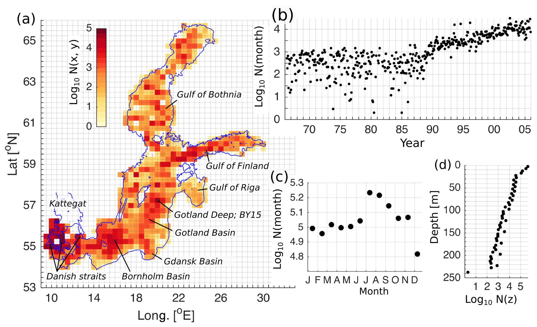
Figure 1 Spatial (a), temporal (b), seasonal (c), and vertical (d) distribution of the number of measurements in the dataset. The horizontal bins have a resolution of 25 km × 25 km (a), temporal and seasonal bins have a monthly resolution (b, c), and vertical bins have a resolution of 5 m (d).

The Baltic Sea (Fig. 1a) is a wide non-tidal estuary-type marginal sea with a longitudinal salinity between 0 and 20 g kg⁻¹ (Leppäranta and Myrberg, 2009; Omstedt et al., 2014). General circulation in the Baltic Sea is cyclonic due to pressure gradient forcing (Meier, 2007). The longitudinal salinity gradient is maintained by saline water inflows from the North Sea through Danish straits and freshwater input by rivers. Large volumes of saline water are transported to the Baltic Sea by the Major Baltic Inflows (MBIs) that occur seldom (Mohrholz, 2018). The other smaller inflows occur almost every winter (Mohrholz, 2018; Raudsepp et al., 2018). Due to gravitational flow, inflowing saline water spreads downstream into the Baltic Sea along the cascade of deep basins – the Bornholm Basin, the Gdansk Basin, and the eastern Gotland Basin. Saline water mixing with fresh water inflow from the rivers forms a Baltic haline conveyor belt (Döös et al., 2004). The saline water of the Gotland Basin is pushed into the western Gotland Basin and the Gulf of Finland. During the MBIs, dense inflow water spreads along the bottom, while other large volume inflows renew the halocline layer of the Baltic Sea. The permanent halocline in the Baltic Sea is at a depth of 60–80 m (Väli et al., 2013). The Gulf of Bothnia and the Gulf of Riga do not have a permanent halocline (Raudsepp, 2001). The Gulf of Finland has a very dynamic halocline due to intensive estuarine circulation (Maljutenko and Raudsepp, 2019), occasional stratification collapses due to reverse estuarine circulation (Elken et al., 2014; 2003), and winter mixing. A seasonal thermocline at a depth range of 10–30 m starts to develop in spring, reaches its maximum strength in summer, and erodes in autumn. In the gulf-type regions of freshwater influence, like the Gulf of Finland (Maljutenko and Raudsepp, 2019) and the Gulf of Riga (Soosaar et al., 2014), the seasonal thermocline coincides with seasonal halocline in spring and summer. During maximum river runoff in spring, river bulge affects the salinity distribution in the coastal sea (Soosaar et al., 2016; Maljutenko and Raudsepp, 2019). In general, the wind-driven and thermohaline circulation of the Baltic Sea and the water exchange with the North Sea determine the stratification in the Baltic Sea (Lehmann and Hinrichsen, 2000).

Salinity fronts are formed in the straits that connect different sub-basins of the Baltic Sea: between Kattegat and southwestern Baltic Sea, the Gulf of Riga and the Baltic Proper, and the Gulf of Bothnia and the Baltic Proper. The Danish straits and Kattegat are situated in a region with a very dynamic and strong front that separates the brackish Baltic Sea water and the saline North Sea water (Nielsen, 2005). The Baltic Sea water of low salinity is transported towards the North Sea in summer, but saline water of the North Sea inflows to the Baltic Sea in winter (Mohrholz, 2018). A dynamic front is present in the transition area between the northeastern Baltic Proper and the Gulf of Finland, although that is a wide and deep area.

The Baltic Sea is seasonally ice-covered. Inter-annually variable and dynamic ice coverage (Raudsepp et al., 2020) has a considerable effect on the evolution of the thermohaline fields in the Baltic Sea.

2 Materials and methods

2.1 Model simulation

The General Estuarine Transport Model (GETM; Burchard and Bolding, 2002) is a numerical 3D circulation model initially developed for coastal and estuarine applications (Gräwe et al., 2015; Holtermann et al., 2014). The hindcast simulation of the general circulation of the Baltic Sea was carried out for the period of 1966–2006 (Maljutenko and Raudsepp, 2019; 2014). The model open boundary was located in Kattegat, where sea-level elevation, temperature, and salinity are prescribed. Model horizontal resolution was set to 1 nmi (1852 m), which was consistent with the horizontal resolution of the digital bathymetry of the Baltic Sea (Seifert and Kayser, 1995). Vertically, 40 bottom-following adaptive layers were used, which resulted in a vertical resolution of less than 5 m.

The initial conditions of salinity and temperature were compiled using observation data from the Baltic Environmental Database (BED; http://nest.su.se/bed, last access: 21 January 2022) (Gustafsson and Medina, 2011; Wulff et al., 2013). Atmospheric forcing was prepared from the BaltAn65+ reanalysis dataset (Luhamaa et al., 2011). The heat fluxes are parameterized using bulk formulation (Kondo, 1975). Monthly river runoff data from the 37 largest rivers from the E-HYPE hydrology model (Donnelly et al., 2016) were used. We have stored daily mean values of temperature and salinity and used them for the analysis.

2.2 Dataset

We use salinity and temperature measurements for the Baltic Sea from the EMODnet Chemistry database (SMHI, 2018). From the original dataset, we have extracted 1 376 674 measurements, which met the following conditions: (1) time range of 1966–2005; (2) spatial range of the model domain, excluding coastal observations, which fell outside the model grid; (3) the simultaneous existence of S and T values; (4) S in the range of 0…35 g kg⁻¹; and (5) T in the range of −2.5…30 ^∘C.

The spatial and temporal distribution of the validation data is presented in Fig. 1. The spatial density of the data is visualized on the 25 km² grid (Fig. 1a). Spatially, there are only a few horizontal cells of 25 km² that do not have any measurements. Vertically, the number of measurements decreases monotonically from the surface to the bottom following the hypsographic curve of the Baltic Sea (Jakobsson et al., 2019) (Fig. 1d). The measurements at the standard depth stick out from the overall curve. Since the end of the 1980s, the number of monthly measurements has increased continuously more than an order of magnitude compared to the preceding period (Fig. 1b). Seasonally, the number of winter and early spring measurements is smaller than the number of summer measurements (Fig. 1c). Gathering data during winter is very complicated due to seasonal ice coverage of the Baltic Sea (Raudsepp et al., 2020).

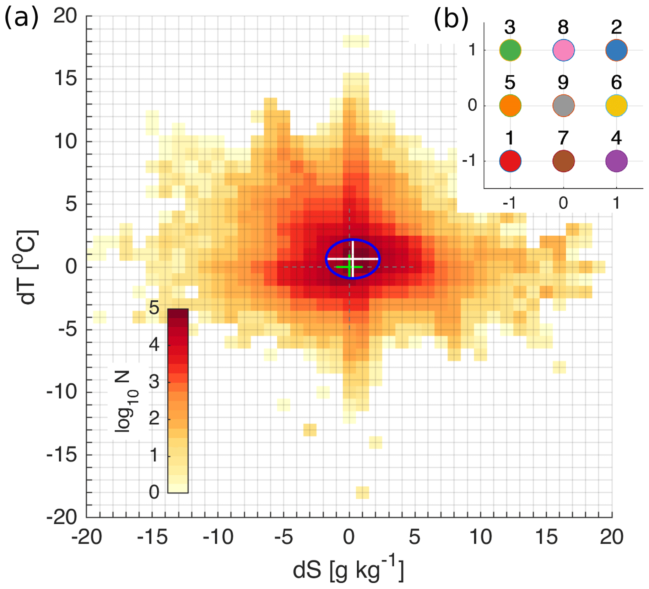
Figure 2 Logarithmic distribution of the number of salinity and temperature error pairs (model minus observation) in the 2-dimensional error space (a). Error bins have a resolution of 1 ^∘C for temperature and 1 g kg⁻¹ for salinity. The bias is shown with the centre of the white cross and the standard deviations with the major semi-axes of the blue ellipse. The green cross shows the centre of the coordinate axes. Coordinates of initial centroids of K-means in the normalized 2-dimensional error space (b).

2.3 K-means clustering

The K-means clustering algorithm is a widely used algorithm in unsupervised machine learning (Hastie et al., 2009; Jain, 2010). We use a K-means clustering algorithm for the cluster analysis of temperature and salinity errors. In the current study, two-dimensional error space is defined from simultaneous salinity and temperature errors {dS,dT} ∈ R², where dS ≡ (S_mod − S_obs) and dT ≡ (T_mod − T_obs). In general, the method can be extended to the n-dimensional error space. The distribution of the errors in the {dS,dT} ∈ R² error space is presented in Fig. 2a. Before calculating K-means, the error space has been normalized by the standard deviation of temperature and salinity errors.

The first step of the method is to determine the number of clusters and an initialization. For practical reasons (Hastie et al., 2009), a regular pattern of initial centroids was chosen for this study (Fig. 2b), although we have run the algorithm with randomly spaced clusters. When we start with only one cluster, we can choose its location at {dS = −1, dT = −1}. Using two clusters means that we start with the locations corresponding to 1 and 2 marked on Fig. 2b. With the increase in the number of clusters, we use corresponding initial locations of the clusters marked with numbers 1, 2, and 3, etc. Other more advanced methods for the selection of initial centroids (Celebi et al., 2013) could be implemented just as well. The squared Euclidean distance was used as the measure of the distance between data points and the centroid coordinates of the cluster. The squared Euclidean distance measured from the cluster centroid is the most commonly used partitioning criterion for continuous data (e.g. Kononenko and Kukar, 2007; Hastie et al., 2009). For practical reasons, the number of iterations was limited to 100, which ensured the convergence of the clustering algorithm. A disadvantage of the K-means clustering algorithm is the lack of a unique way of defining the optimal number of clusters. For the final selection of the number of clusters, we used the Elbow method (e.g. Bholowalia and Kumar, 2014; Yuan and Yang, 2019). The coordinates of the centroids in {dS,dT}error space provide mean bias of the errors belonging to the cluster k. Standard deviations of dS and dT are calculated for the characterization of the variability of the errors within a cluster.

In general, the errors retain their 4-dimensional structure, i.e. {dS,dT} $(t,x,y,z)$, while assigned to specific clusters. Any kind of analysis can be done using the clustered errors.

2.4 Normalization

Each error pair belongs to a fixed cluster k but retains their 4-dimensional structure, i.e. {dS,dT}^k $(t,x,y,z)$. For the visualization of model accuracy, some reduction of dimensionality of the error pairs is needed.

For the spatial distribution of errors, we take the error pairs as independent of time and vertical coordinate, i.e. {dS,dT}^k (x,y). For each horizontal grid cell (i,j) of 25 km², we have a number of points (error pairs) $n_{i,j}^k$ that belong to cluster k. The total number of points that belong to the grid cell is $N_{i,j}={\sum }_{k=\mathrm{1}}^K{n}_{i,j}^k$, where K is the number of clusters. For normalization, we divide each $n_{i,j}^k$ by N_i,j and plot the horizontal maps for each k.

For the vertical distribution of errors, we take error pairs as dependent only on the vertical coordinate {dS,dT}^k (z). Then $n_l^k$ is the number of points in layer l and cluster k. The total number of points in the layer l is $N_l={\sum }_{k=\mathrm{1}}^K{n}_l^k$. Normalization is done for each layer with N_l. Subsequently, the profiles of the normalized error points show the share of each cluster of errors.

For the temporal distribution of errors, we take error pairs as dependent only on time {dS,dT}^k (t). Then $n_{\mathrm{\Delta }t}^k$ is the number of points in the time interval Δt and cluster k. The total number of points in the time interval Δt is $N_{\mathrm{\Delta }t}={\sum }_{k=\mathrm{1}}^K{n}_{\mathrm{\Delta }t}^k$. Normalization is done for each time interval Δt with N_Δt. Then the time series of the normalized error points shows the share of each cluster of errors at a specific time.

There is no need to do normalization when we look at time series in a fixed spatial location or plot the Hovmöller diagram of error clusters.

Table 1 The coordinates of the centroids and the standard deviations of salinity and temperature errors within the clusters for a different set of predefined number of clusters, K = 1–9. The numbers in column k correspond to the index of the clusters in Fig. 3 for corresponding set of K clusters. The numbers in column k(K=4) refer to the indices of the corresponding clusters of the case K=4.

Figure 3 The distribution of clusters in the error space for a different number of predefined clusters, K = 1–9. The numbers of the clusters correspond to the numbers of the clusters in Table 1. The biases are marked with the centre of the ellipsoid and the standard deviations with the major semi-axes. The error space has been zoomed in for better visualization of the clusters. The full range of error space and distribution of the clusters is shown in Fig. A1 in Appendix A.

3 Results

3.1 Clustering procedure

We start by clustering bulk data covering the entire modelling period and domain. Error representation does not provide a clear understanding on how many clusters should be predefined or how the clusters will form. The initial location of the centroids is selected according to the scheme shown on Fig. 2b. The coordinates of the centroid of one cluster (Fig. 3a) provide a model bias of 0.64 ^∘C for temperature and 0.26 g kg⁻¹ for salinity (Table 1). The corresponding standard deviations were 1.5 ^∘C and 2.0 g kg⁻¹, respectively. The root mean square difference was 1.67 ^∘C for temperature and 2.04 g kg⁻¹ for salinity. The corresponding linear correlation coefficients were 0.97 and 0.95, respectively.

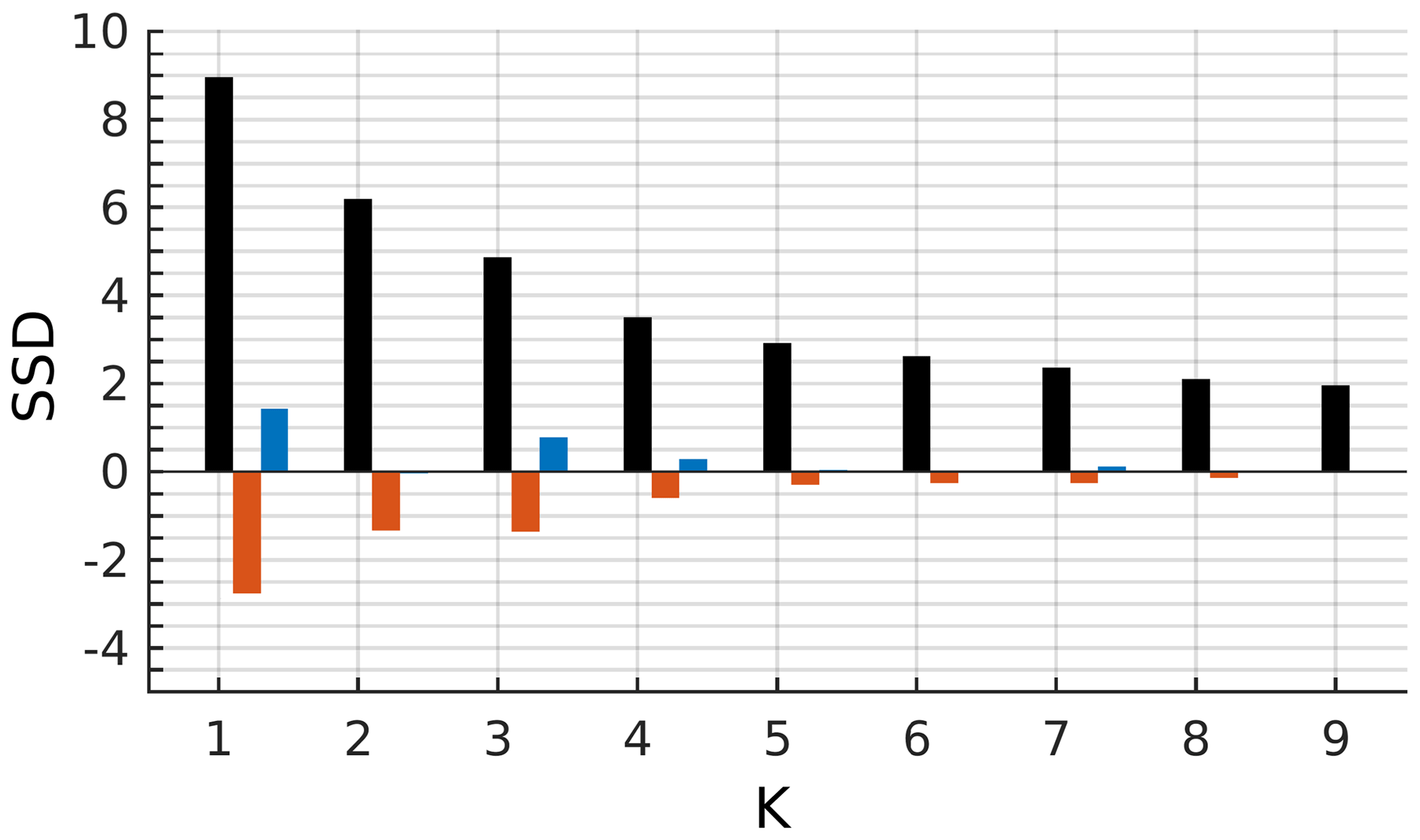
Figure 4 Sum of square distances (black bars) between the normalized pairs of error points and their designated centroids for different numbers of initial centroids. The first-order (red bars) and the second-order (blue bars) forward differences calculated from the sum of square distances.

Increasing the number of clusters results in the splitting of the error space into clusters with centroids close to the zero point (Fig. 3). A representative structure of distribution of the errors emerges in the case of four clusters (Fig. 3d). We can confirm the choice of four clusters by implementing cluster selection criteria. The distance between points and designated centroids reduces exponentially with the increase in the number of clusters (Fig. 4). The rate of distance reduction with the increasing number of clusters shows local minima at K=4.

The K=4 clustering distributes 1 376 674 error data pairs into the following four clusters, each with N(k) = {263 230, 196 615, 134 326, 782 503} data points. Cluster k=1 characterizes the set of errors with the basic feature of “underestimated salinity” (Table 1). This cluster is present already in the case of three clusters (Fig. 3c). Increasing the number clusters splits this cluster into two clusters (e.g. for K=9, it splits into clusters $k=\mathrm{1},\mathrm{5}$). Cluster k=2 envelops the errors of “overestimated salinity”. This cluster changes into cluster k=4 (K=5), then splits into two clusters (K=8) and three clusters (K=9). Cluster k=3 of “overestimated temperature” is established already in the case of three clusters. Increasing the total number of clusters does not result in a split of the cluster. However, the centroid shifts towards a high temperature bias (Table 1). The cluster k=4 represents a “good match” of the model and measurements. The bias is about 0.4 ^∘C for temperature and 0.6 g kg⁻¹ for salinity (Table 1). The standard deviations are below 1 for both parameters. Increasing the number of clusters results in the splitting of this cluster along the axis of temperature error, while the salinity error remains small.

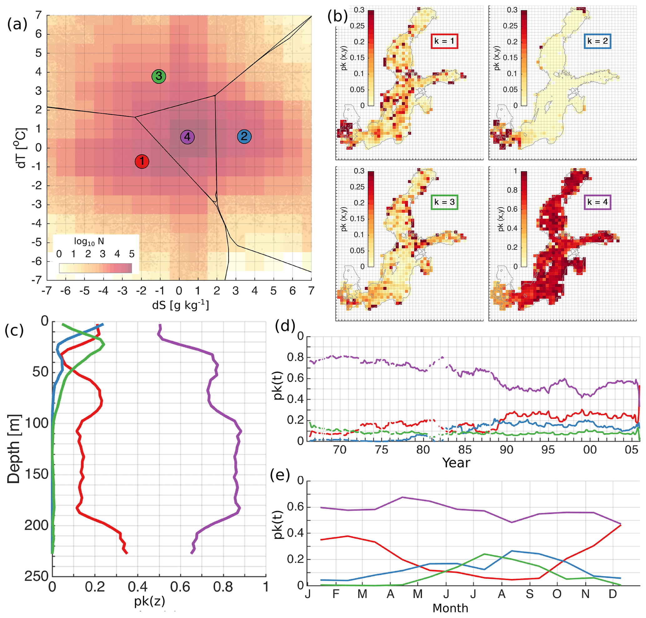
Figure 5 The distribution of the error clusters for K=4 (a). The coloured map shows the logarithmic distribution of the number of salinity and temperature error pairs (model minus observation) in the 2-dimensional error space (a). Error bins have a resolution of 1 ^∘C for temperature and 1 g kg⁻¹ for salinity (a). The spatial (b), vertical (c), temporal (d), and seasonal (e) distribution of the share of error points belonging to the four different clusters (b). The share, p(k), representing the share of the error points belonging to the cluster k, is calculated as explained in Sect. 2.4. The horizontal bins have a resolution of 25 km × 25 km (b), vertical bins have a resolution of 5 m (c), and temporal and seasonal bins have a monthly resolution (d, e). The lines in (d) have been smoothed using a running mean with a 12-point window size. Line colours correspond to the colours of the clusters in (a).

3.2 Analysis of the clusters

Retrieving spatial coverage of K=4 cluster errors shows that the model has a good match in the whole model domain (Fig. 5b). The share of the other errors remains less than 0.3. The model overestimates salinity, underestimates salinity and has a good match at the Danish straits. Underestimated salinity errors have a share of about 0.2 in the deep basins of the Baltic Proper, i.e. the Bornholm Basin, Gdansk Basin, eastern Gotland Basin, northern Baltic Proper, western Gotland Basin, and western Gulf of Finland. The model overestimates temperature at the transition area between the northeastern Baltic Proper and the Gulf of Finland, in some coastal locations, and within river plumes. The latter indicates that river water temperature is overestimated in the present model implementation.

Vertical distribution of the error clusters confirms that the share of good match errors ranges between 0.5 and 0.9 of all data (Fig. 5e). In the surface layer, we have overestimated salinity and underestimate salinity in almost 50 % of cases. In comparison with horizontal distribution of errors, a large part of these errors probably belongs to the Danish straits (Fig. 5b). The overestimated temperature has a considerable share centred at a depth of 25 m. The underestimated salinity has a high share at the depth range of 60–100 m. The share of underestimated salinity once again increases in the deep layer of the Baltic Sea.

A decrease in time of a good match coincides with an increase of the share of underestimated salinity and overestimated salinity (Fig. 5c). Seasonally overestimated salinity has a higher share in summer, while underestimated salinity has a higher share in winter (Fig. 5d). Combining the horizontal (Fig. 5b) and seasonal distribution of errors (Fig. 5d), we could conclude that the salinity is overestimated in the Danish straits in summer and underestimated in winter. In addition, we would like to note that the good match share decreases and underestimated salinity increases abruptly at the end of the 1980s when the number of measurements becomes larger in the database. The overestimated temperature has an almost constant share of 0.1 in time (Fig. 5c). The elevated share of overestimated temperature errors in summer confirms that the model overestimates the temperature in the seasonal thermocline (Fig. 5d). For comparison, we have provided a similar analysis of the errors for K=3 and K=5 in Appendix B.

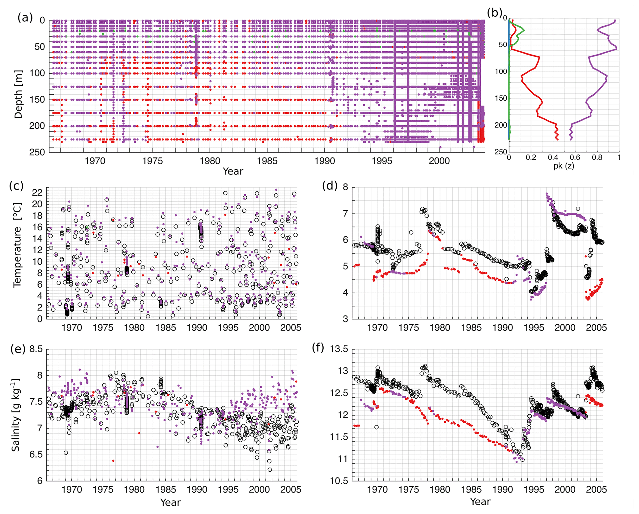
Figure 6 Hovmöller diagram of the distribution of error points of K=4 at the BY15 monitoring station (a). Vertical distribution of the share of error points belonging to the four different clusters (b). The share, p(k), representing the share of the error points belonging to the cluster k, is calculated as explained in Sect. 2.4. Time series of observed (black circles) and simulated (colour dots) temperature (c, d) and salinity (e, f) on the surface (c, e) and bottom (d, f) at the BY15. Colours of dots and lines correspond to the colours of the clusters in Fig. 5a.

We extract error profiles from Gotland Deep station BY15, which is widely used for the validation of the physical and biogeochemical models of the Baltic Sea. In the upper layer of 60 m, the model has a good match (Fig. 6a and b). There are isolated occasions of 10 % in total when the model overestimates temperature in the seasonal thermocline (Fig. 6b). At the depth range 60–100 m, the share of model underestimating salinity increases. From a depth of 100 m, the proportion of the model that underestimates salinity gradually increases with depth. The Hovmöller diagram shows that there are extended time periods when the model underestimates salinity (Fig. 6a). In the surface layer, the model has a good match, although model salinity starts to deviate from the measurements from 1995 onwards (Fig. 6c and e). At the bottom, the model reproduces temperature very well at the end of the 1970s and the beginning of the 1980s, but as salinity is underestimated, the errors belong to the cluster of underestimated salinity (Fig. 6d and f). In general, the model has a good match in the water column from 1991 to 2003 (Fig. 6a and f). Dynamically, this corresponds to the end of the stagnation period and recovery of the bottom salinity and strengthening of the permanent halocline.

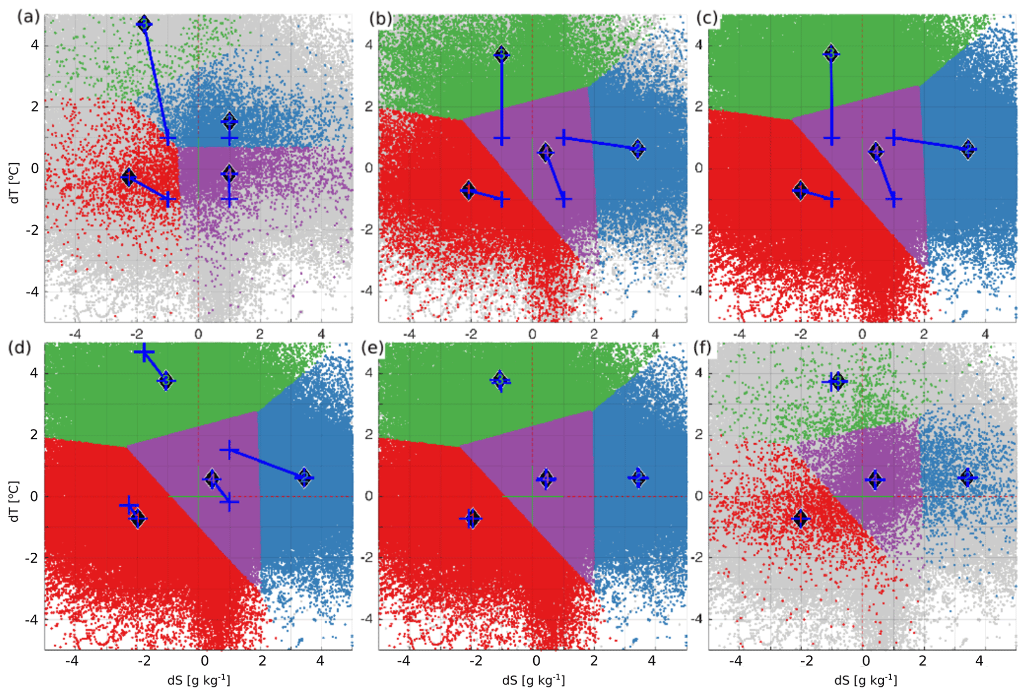
Figure 7 Learning (a–c) and predicting (d–f) of the K=4 clusters. The learning and predicting datasets have a share of 1 % (a) and 99 % (d), 20 % (b) and 80 % (e), and 99 % (c) and 1 % (f) of the full dataset, respectively. Blue crosses mark the location of initial centroids and blue lines connect initial and final locations (marked with numbered diamonds) of the centroids.

3.3 Learning of the clusters

As the first step, the whole 4-dimensional {dS,dT}dataset is divided randomly into two separate sets for learning and predicting. The dataset for the learning of the error clusters is initiated from a set of a different number of clusters according to initial distribution of the centroids shown on Fig. 2b. Resulting centroids of the learning dataset are then used to initiate the centroids for the clustering of the predicting dataset. The mean length of shifts between learning and predicting centroids is used to evaluate the effect of dataset size on predicting the representative error clusters. We have used different learning and predicting datasets with sizes ranging from a share of 10⁻⁴ to 0.9999 of the total dataset of 1 376 674 error pairs. For a statistical ensemble of randomly selected datasets, the average distances are calculated from 30 trials. The learning and predicting procedure is illustrated in Fig. 7 for K=4.

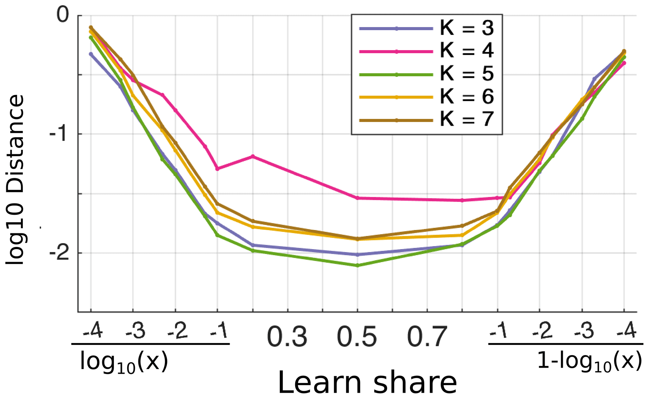
Figure 8 The average normalized distance of shifts of predicting centroids relative to learned centroids as a function of the share of the learning dataset. Averaging has been done from 30 trials. Different lines correspond to different numbers of initial clusters, K = 3–7. The share of the learning dataset in the ranges of 10⁻⁴–0.1 and 0.9–0.9999 is shown on a logarithmic scale.

If the learning dataset makes up 10 %–95 % of the total dataset (> 100 000 comparison points), then the difference between the learned and predicted centroids does not change significantly (Fig. 8). The clustering of K=4 is most sensitive to the choice of initial centroids. Therefore, the distance between learned and predicted centroids is larger compared to other choices of K. Below 1 % of the learning data size (< 10 000 comparison points), the difference in distance between learned and predicted datasets is > 0.03 normalized standard deviation. Thus, the size of the learning dataset is significant for predicting the error clusters. The rough estimate of the number of comparison points is about 100 000 for the current model, which shows relatively stable centroids and the stability of the model accuracy.

3.4 Interpretation of the clusters

The total number and the spatio-temporal coverage of the comparison points (Fig. 1) indicate that the model performs well over the Baltic Sea and the simulation period considered (Fig. 5). The share of model errors with a bias of {dS,dT} = {0.44 g kg⁻¹, 0.57 ^∘C} and with a standard deviation of {dS,dT} = {0.69 g kg⁻¹, 0.81 ^∘C} (Table 1) is between 0.5 and 0.9.

In addition, we can highlight the areas where the model accuracy is lower and the dynamical features are not so well reproduced by the model. Essentially, the seasonal thermocline and permanent halocline are not reproduced by the model as well as the layers with small vertical gradients of salinity and temperature. The accuracy of the model in reproducing a seasonal thermocline has a peak share of overestimated temperature of 0.25 (bias of 3.78 ^∘C and standard deviation of 1.73 ^∘C) at a 25 m depth. The error share of 0.25 is observed in the layer of 60–90 m, which corresponds to the depth range of the permanent halocline. The model underestimates salinity (bias of −1.96 g kg⁻¹ and standard deviation of 1.63 g kg⁻¹) there.

Model accuracy is relatively low in the Danish straits. The model has underestimated salinity in winter and overestimated salinity in summer (bias of 3.44 g kg⁻¹ and standard deviation of 1.59 g kg⁻¹) there. The underestimated salinity errors in the deep basins of the Baltic Sea (Fig. 5b) are caused by the spreading of inflowing North Sea water downstream in the cascade of the deep basins. These inflows mainly take place in winter, while outflow of the Baltic Sea water dominates in summer.

Clustering of model errors could provide information about the accuracy of external fields that are used for the forcing and for the boundary conditions of the model. The overestimated temperature at the river plume areas (Fig. 5b) may indicate a mismatch of river water temperature that takes the value from a grid cell adjacent to the river mouth. Although the air–sea fluxes are correctly reproduced by the model, as indicated by a good match at the surface (Fig. 5c), the following downward flux of heat could be too strong, as the share of overestimated temperature is relatively high between the depth of 10–40 m in summer (Fig. 5c and d).

4 Summary

Ideally, researchers like to know the model accuracy over the whole model domain and time period simulated. Commonly used methods provide a limited set of metrics (e.g. bias, standard deviation, root mean square error, correlation coefficient) for the assessment of overall quality of the model. In this study, we have proposed a new method for the assessment of model skills. The aim of using the method is the clustering of multivariate model errors. Model errors consist of differences between model values and the measured multivariate data. The main advantage of this method is the possibility to use clustered errors for the analysis of the spatio-temporal accuracy of the model.

The method was tested in the validation of the circulation model results of the 40-year period in the Baltic Sea. Temperature and salinity were used for validation because they are essential parameters of the physical model, and these data have been the most extensively measured in the Baltic Sea. This method enables us to use all available observations, with the only restriction being the need to measure multivariate data simultaneously. In model validation, the problem usually lies in the spatio-temporal distribution of measurement data over the 4-dimensional model domain. In our case, the measurement data were sufficient and had good spatial and temporal coverage. In total, we had more than 1 300 000 pairs of measured temperature and salinity values. In many cases, reduction of available data or homogenization of the data is needed prior to the calculation of model errors, and clustering is applied to have simultaneous multivariate data. The number of measurements should be sufficiently large to determine stable clusters. In our case, about 100 000 randomly selected data pairs showed relatively stable centroids and the stability of the model accuracy.

We have applied the K-means unsupervised machine learning algorithm for the assessment of the quality of general circulation models by clustering temperature and salinity errors. The model output fields are 4-dimensional, and the 4-dimensional distribution of the errors was retained after the clustering was completed. As a result, cluster numbers were assigned to each error pair. In addition, the errors belonging to one cluster had their bias determined by the location of the centroid in the error space. Further on, common statistical metrics (e.g. standard deviation, root mean square error, correlation coefficient) can be calculated for each cluster and variable. In general, any other partitional clustering algorithm can be used instead of K-means for the clustering of multivariate model errors. Although the tests with the balanced iterative reducing and clustering using hierarchies (Zhang et al., 1996), the Gaussian mixture model, and K-nearest-neighbour algorithm (e.g. Hastie et al., 2009) were performed (results not shown), we have implemented the K-means algorithm because of its simplicity and robustness. The outcome clusters have direct information on the model bias. The output clusters can be used for the calculation of classical statistical metrics. The resulting clusters contain information about common statistical metrics.

The K-means clustering algorithm has a well-known deficiency. There is no unique way to determine the number of clusters. We used Elbow methods, which gave good results. The selection of four clusters was supported by the analysis of the error clusters in relation to the geographical distribution of the errors, the physical process, and the features. The analysis showed that the underestimated salinity cluster was mainly in the Danish straits, within the halocline layer and along the pathway of transport of saline water in the Baltic Sea. Overestimated temperature had a high share in the seasonal thermocline. Overestimated salinity accounted for the model errors in the Danish straits. For confidence, the analysis was complemented with the use of three and five clusters. Thus, the analysis of the error clusters enables us to shed light on the physical processes and features where model performance should be improved.

The clustering was done for the entire Baltic Sea and the whole simulation period. In comparison, conventional model validation with station measurements of temperature and salinity is presented in Maljutenko and Raudsepp (2014, 2019). The analysis of clusters of errors at specific locations enables us to assess the quality of the model at these locations in the context of the overall quality of the model. Multivariate model quality assessment shows that if one parameter is well reproduced by the model but the other parameter is poorly reproduced at the same time, then the quality might not be good.

In addition to model quality, error clustering can provide implicit information about the quality of prescribed input variables and forcing fields. Error clustering has shown that the temperature of river runoff water could be overestimated. This is especially relevant in the case of biogeochemical models, where discharges of different nutrients and other state variables, which have to be prescribed, are usually poorly known. There are problems in the prescribed salinity of the inflowing North Sea water at the open boundary of the model in the Kattegat. In addition, these errors are transported into the model domain of southwestern Baltic Sea. However, atmospheric fields necessary for the calculation of the air–sea heat fluxes do not produce significant errors. The proposed method could be applied for the assessment of the quality of global ocean general circulation models. By the end of the year 2020, there were approximately 3800 ARGO floats profiling the world ocean for salinity and temperature, with a spatial resolution of approximately one float for every 3^∘ of latitude and longitude. The annual total number of profiles added to the database is over 100 000, which takes the total available number of profiles to over 2 000 000 (Argo, 2020). This huge validation dataset probably needs some computational solution, i.e. implementation of parallel computing or specific methods on how to deal with big data within the K-means clustering. In the context of operational oceanographic models, the model validation can be done in “real time” by implementing the learning–predicting sequence. The ARGO data, which are available within 24 h of collection, could be added to the learned clusters for the updating of the coordinates of centroids and statistical metrics.

The proposed method can be applied to different geoscientific models. The shortlist consists of biogeochemical models, atmospheric models, wave models, hydrological models, and geodynamic models. An application of the method for the assessment of a coupled physical and biogeochemical model of the Baltic Sea is presented in Kõuts et al. (2021). The method can be implemented in a multivariate high-dimensional error space as well as in a univariate error space. In addition to the validation of numerical models, the method can be used for the assessment of remote-sensing data and models.

Appendix A

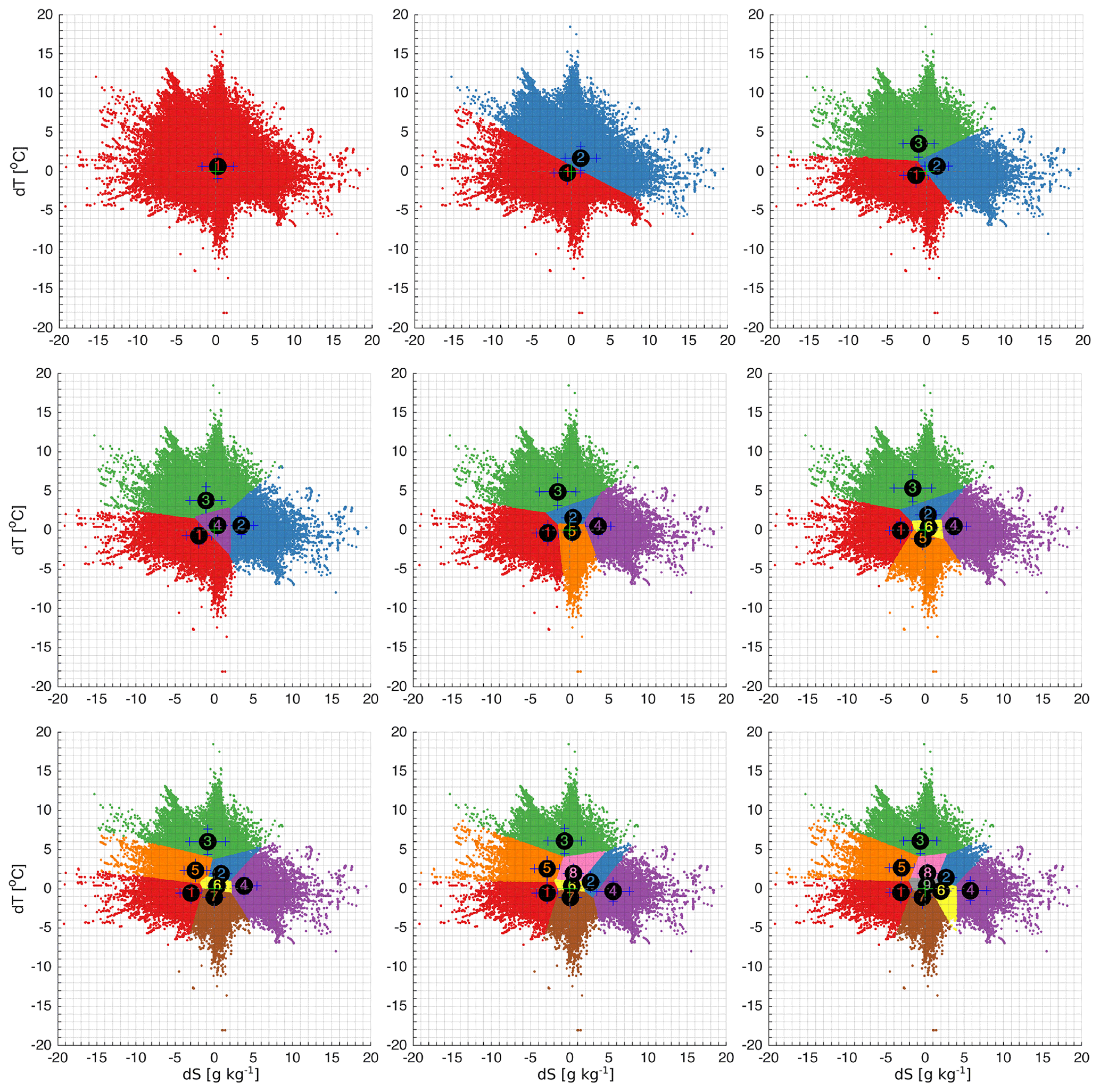
Figure A1 The distribution of clusters in the error space for a different number of predefined clusters, K = 1–9. The numbers of the clusters correspond to the numbers of the clusters in Table 1. The locations of the centroids are marked with cluster numbers and the standard deviations with the whiskers.

Appendix B

In the case of three clusters, the largest share of errors belongs to the cluster k=2 with a bias of {dS,dT} = {1.3 g kg⁻¹, 0.66 ^∘C}and with a standard deviation of {dS,dT} = {1.52 g kg⁻¹, 0.85 ^∘C} (Fig. B1). This cluster provides the main contribution to the good match and overestimated salinity clusters when a larger number of clusters is used. The share of the errors of this cluster is between 0.6 and 0.9. Cluster k=1 with a bias of {dS,dT} = {−1.35 g kg⁻¹, −0.51 ^∘C} and with a standard deviation of {dS,dT} = {1.57 g kg⁻¹, 0.99 ^∘C} is the cluster of underestimated salinity, which retains these features throughout the increasing of the number of clusters. Spatially, underestimated salinity has a significant share in the Danish straits and on the pathway of inflowing saline water through the deep basins of the Baltic Sea. Vertically, these errors have a large share of 0.5 in the layer of 60–110 m, which corresponds to the permanent halocline of the Baltic Sea, and below 200 m, which is the bottom layer of the Gotland Deep. The share of underestimated salinity is relatively high in the whole water column below the halocline. Seasonally, these errors are significant in winter, when saline water inflows through the Danish straits to the Baltic Sea occur. Cluster 1 with a bias of {dS,dT} = {−1.03 g kg⁻¹, 3.54 ^∘C} and with a standard deviation of {dS,dT} = {1.97 g kg⁻¹, 0.73 ^∘C} has a steady share of errors of 0.1. The errors of overestimated temperature are significant in the depth range of 10–50 m and during summer. These errors account for the model accuracy in reproducing the seasonal thermocline.

In the case of five clusters, the clusters k=2 with a bias of {dS,dT} = {0.42 g kg⁻¹, 1.54 ^∘C} and with a standard deviation of {dS,dT} = {0.95 g kg⁻¹, 0.66 ^∘C} and k=5 with a bias of {dS,dT} = {0.3 g kg⁻¹, −0.22 ^∘C} and with a standard deviation of {dS,dT} = {0.72 g kg⁻¹, 0.77 ^∘C} dominate over the others (Fig. B2). These clusters are formed as a split of the good match cluster with partial contribution from the underestimated salinity cluster and the overestimated salinity cluster of K=4. The clusters k=1 with a bias of {dS,dT} = {−2.81 g kg⁻¹, −0.37 ^∘C} and with a standard deviation of {dS,dT} = {1.42 g kg⁻¹, 1.07 ^∘C} and k=4 with a bias of {dS,dT} = {3.63 g kg⁻¹, 0.52 ^∘C} and with a standard deviation of {dS,dT} = {1.63 g kg⁻¹, 1.08 ^∘C} share errors of underestimated salinity and overestimated salinity. These errors dominate in the Danish straits, indicating the difficulties for the model in matching fluctuating water salinity close to the model boundary. Cluster k=3 with a bias of {dS,dT} = {−1.52 g kg⁻¹, 4.89 ^∘C} and with a standard deviation of {dS,dT} = {2.33 g kg⁻¹, 1.76 ^∘C} accounts for overestimated temperature errors in the seasonal thermocline during summer.

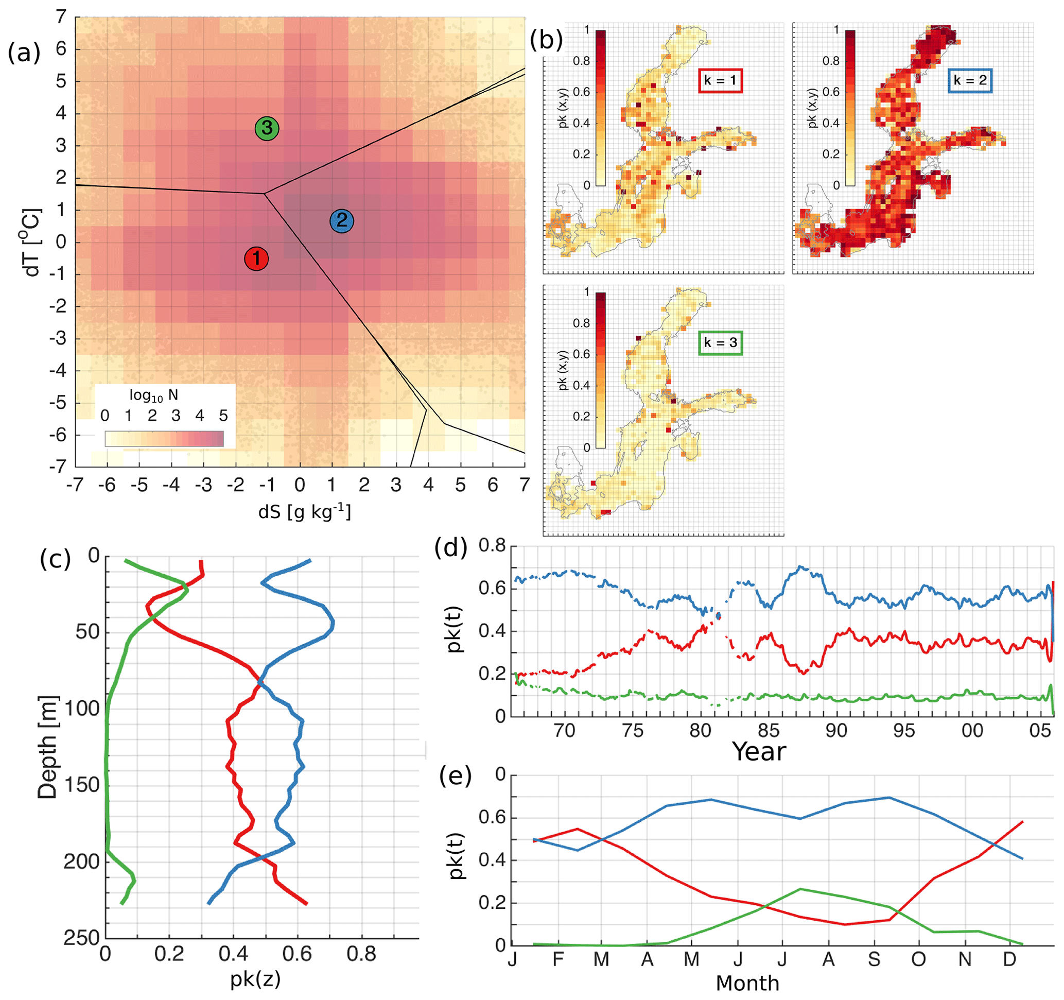
Figure B1 The distribution of the error clusters for K=3 (a). The coloured map shows logarithmic distribution of the number of salinity and temperature error pairs (model minus observation) in the 2-dimensional error space (a). Error bins have a resolution of 1 ^∘C for temperature and 1 g kg⁻¹ for salinity (a). The spatial (b), vertical (c), temporal (d), and seasonal (e) distribution of the share of error points belonging to the four different clusters (b). The share, p(k), representing the share of the error points belonging to the cluster k, is calculated as explained in Sect. 2.4. The horizontal bins have a resolution of 25 km × 25 km (b), vertical bins have a resolution of 5 m (c), and temporal and seasonal bins have a monthly resolution (d, e). The lines (d) have been smoothed using a running mean with a 12-point window size. Line colours correspond to the colours of the clusters in (a).

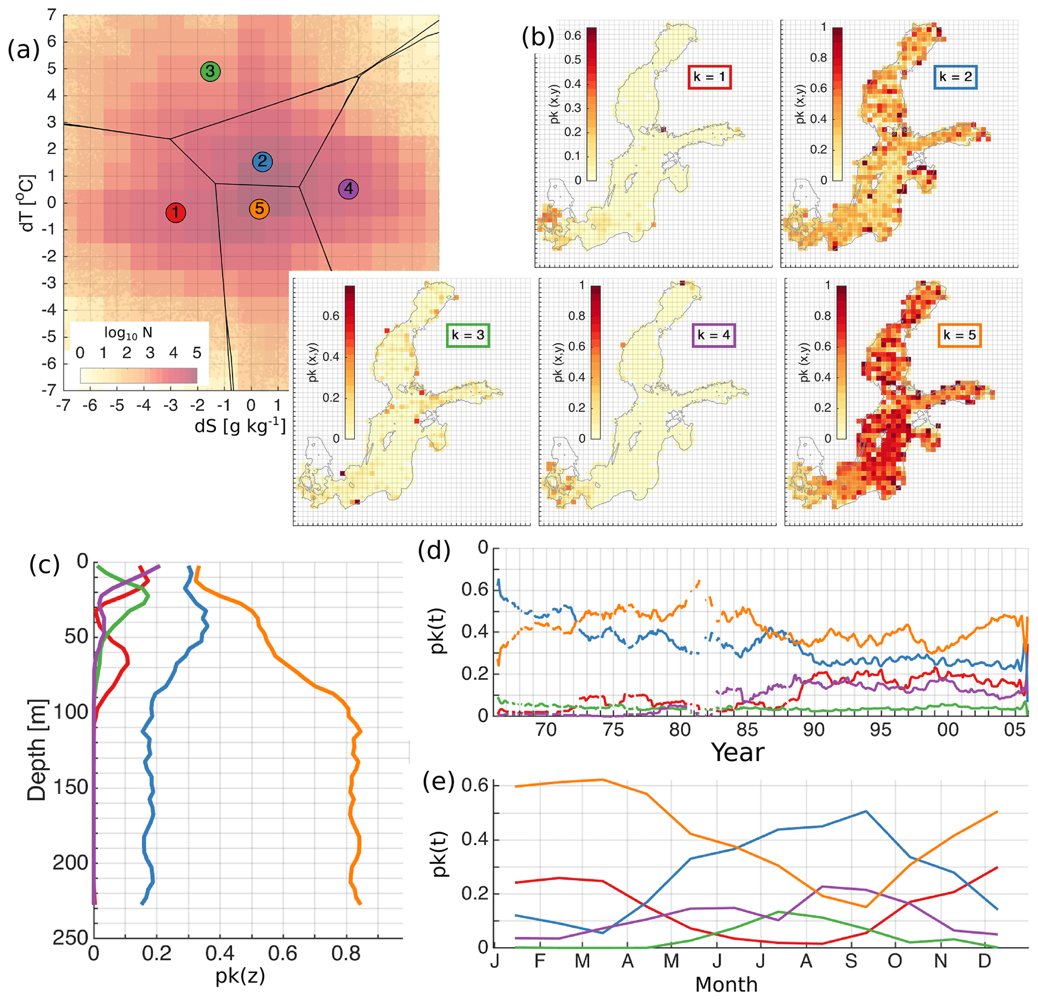
Figure B2 The distribution of the error clusters for K=5 (a). The coloured map shows logarithmic distribution of the number of salinity and temperature error pairs (model minus observation) in the 2-dimensional error space (a). Error bins have a resolution of 1 ^∘C for temperature and 1 g kg⁻¹ for salinity (a). The spatial (b), vertical (c), temporal (d), and seasonal (e) distribution of the share of error points belonging to the four different clusters (b). The share, p(k), representing the share of the error points belonging to the cluster k, is calculated as explained in Sect. 2.4. The horizontal bins have a resolution of 25 km × 25 km (b), vertical bins have a resolution of 5 m (c), and temporal and seasonal bins have a monthly resolution (d, e). The lines (d) have been smoothed using a running mean with a 12-point window size. Line colours correspond to the colours of the clusters in (a).