the Creative Commons Attribution 4.0 License.
the Creative Commons Attribution 4.0 License.
 | 13 Jul 2022
uDALES 1.0: a large-eddy simulation model for urban environments
Ivo Suter
Tom Grylls
Birgit S. Sützl
Sam O. Owens
Chris E. Wilson
Maarten van Reeuwijk
Urban environments are of increasing importance in climate and air quality research due to their central role in the population's health and well-being. Tools to model the local environmental conditions, urban morphology and interaction with the atmospheric boundary layer play an important role for sustainable urban planning and policy making. uDALES is a high-resolution, building-resolving, large-eddy simulation code for urban microclimate and air quality. uDALES solves a surface energy balance for each urban facet and models multi-reflection shortwave radiation, longwave radiation, heat storage and conductance, as well as turbulent latent and sensible heat fluxes. Vegetated surfaces and their effect on outdoor temperatures and energy demand can be studied. Furthermore, a scheme to simulate emissions and transport of passive and reactive gas species is present. The energy balance has been tested against idealised cases and the dispersion against wind tunnel experiments of the Dispersion of Air Pollution and its Penetration into the Local Environment (DAPPLE) field study, yielding satisfying results. uDALES can be used to study the effect of new buildings and other changes to the urban landscape on the local flow and microclimate and to gain fundamental insight into the effect of urban morphology on local climate, ventilation and dispersion. uDALES is available online under the GNU General Public License and remains under active maintenance and development.
- Article
(12905 KB) - Full-text XML
- BibTeX
- EndNote


With an ever-increasing number of people living in cities (UNFPA, 2012), understanding how the urban morphology influences the transport of momentum, heat, moisture and pollutants is central to designing healthy, sustainable and safe urban environments. Indeed, the large number of tall towers being erected in large cities around the world necessitates elaborate studies on how these affect the safety of pedestrians, since these structures can channel high-momentum air down to ground level (Lawson and Penwarden, 1975; Isymov and Davenport, 1975; ASCE, 2004, 2011; Blocken et al., 2003, 2016). Densely populated areas are prone to developing an urban heat island (UHI) effect (increased temperatures relative to the surrounding rural areas, partially due to the limited vegetation and water surfaces; Oke, 1982; Rosenzweig et al., 2015). The UHI increases the intensity of heat waves, with a measurable increase in mortality rates (Pyrgou and Santamouris, 2018). Furthermore, the large concentrations of people in urban areas create problems with urban air quality; it is a sobering fact that health quality standards are exceeded in most of the world’s largest cities, despite the known adverse effects on human health (World Heath Organization, 2021).
The increased likelihood of extreme weather events due to climate change (Seneviratne et al., 2021) and the need to transition to a less carbon-hungry society make our ability to predict the urban climate even more important. Design decisions that are taken now will strongly influence whether we will be able to meet the intentions outlined in the COP agreements (UNFCCC, 2020). The choice of building materials and city layout has to be reconsidered together with intelligent management of water systems and green spaces. Greening of façades and roofs can mitigate the effects of the UHI (Santamouris, 2014); specifically, greening improves thermal comfort and lowers heat stress due to enhanced evapotranspiration from vegetation. Green roofs or walls also lead to lower indoor temperatures and reduce the energy demand for air-conditioning (Castleton et al., 2010). Consequently, the augmented installation of green infrastructure is a possible remedy for exceedingly hot cities and the subsequent health problems (Bozovic et al., 2017).
With business-as-usual emission regulation policies, mortalities due to outdoor air quality will continue to rise in the period up to 2050 (Lelieveld et al., 2015). The “metabolic” consumption of energy and materials within cities results in the presence of a wide range of harmful pollutants in the urban atmosphere (Oke et al., 2017). Long-term improvements in air quality must be driven through reduced emissions. However, (1) this process requires large-scale, long-term infrastructural and behavioural change, and (2) recent studies indicate the complexity and global variability of source contributions (e.g. the importance of non-combustible emission sources; Lelieveld et al., 2015; Grylls, 2020). Short-term and more flexible solutions are therefore also needed; e.g. temporary limitations on transport (Borge et al., 2018), optimised urban design (Llaguno-Munitxa and Bou-Zeid, 2018) and technical innovations for active removal (Sikkema et al., 2015). Accurate predictions of the emission, dispersion, chemical reaction and removal of pollutant species in the urban atmosphere are integral to developing our understanding of and therefore solutions to the global challenge of urban air quality.
Reliable methods to model the interaction between the atmospheric boundary layer and the urban morphology are key to predictions of pedestrian safety, urban microclimate and urban air quality. The urban structure is inherently heterogeneous: roads, residential, commercial and industrial zones segment cities and are interspersed with vegetation and open water. Moreover, the urban fabric, i.e. the material composition and texture of the urban surface, is also subject to great variability. This represents a major challenge to the modelling of urban processes due to their large range of associated spatial and temporal scales.
The complexity of the urban structure and fabric makes computational fluid dynamics (CFD) models a popular modelling choice. Wind engineering models are predominantly based on the Reynolds-averaged Navier–Stokes (RANS) equations, which require turbulence parameterisations for the full range of active scales in the flow field (Blocken, 2015). This allows for the use of relatively large time steps or even steady-state simulations that predict the flow field reasonably well. However, the reliance on turbulence parameterisations requires careful validation and sensitivity analyses (Blocken, 2015). Many RANS codes, including commercial CFD packages (Fluent, ANSYS CFX, COMSOL etc.) and open-source alternatives such as OpenFoam, are capable of simulating flow and dispersion in urban areas. In non-neutral situations, which is the predominant atmospheric state over cities (Barlow, 2014; Kotthaus and Grimmond, 2018), the use of RANS is more problematic due to the influence of buoyancy on the velocity field (Hanjalić and Kenjereš, 2008).
However, most CFD models neither contain a representation of energy exchanges at the urban surface nor explicitly treat radiative fluxes. Coupling of stand-alone energy balance models is a possibility (Musy et al., 2015), yet technical difficulties persist and different approaches in model design exist across numerous research groups. The exceptions are urban climatology models based on the Reynolds-averaged Navier–Stokes (RANS) equation that are able to take into account the thermal exchanges in the urban area, e.g. MIMO (Ehrhard et al., 2000), MITRAS (Schlünzen et al., 2003; Salim et al., 2018), ENVI-met (Huttner, 2012) and MUKLIMO3 (Sievers, 2016).
Large-eddy simulation (LES) tools explicitly resolve the large turbulent scales of the flow that contain the majority of the turbulent energy and are therefore less reliant on turbulence models than RANS. LES is more computationally demanding than RANS. However, the continuous increase in computational resources makes LES models the most promising method to provide sufficiently detailed and accurate information on how the interaction of heat, moisture and momentum exchanges affects the local urban microclimate. Examples of LES models capable of dealing with the urban terrain are PALM-4U (Maronga et al., 2020; Resler et al., 2021) and OpenFoam2. Indeed, PALM-4U has similar goals and many similarities to uDALES. OpenFoam, however, does not offer the possibility to model many features of the urban climate, such as the surface energy balance.
The aim of this paper is to present a new open-source large-eddy simulation model for the urban environment, uDALES (Grylls et al., 2021a). This model is an extension of the atmospheric LES model DALES (Heus et al., 2010; Tomas et al., 2015). uDALES explicitly solves the flow around buildings, includes wet thermodynamics and solves a full surface energy balance including vegetated surfaces. It can be used to model both the standard idealised flow cases that are pursued in air quality studies (Caton et al., 2003) and realistic case studies (Grylls et al., 2019). uDALES is capable of solving a surface energy balance in a two-way coupled manner with the flow and models the dominant processes that characterise the urban environment, such as radiation, the effect of vegetation, and energy and momentum fluxes from urban surfaces. uDALES is set up in a modular fashion that makes it relatively straightforward to add additional modules.
The paper is structured as follows. In Sect. 2 the fundamentals of the model are outlined and the treatment of boundary conditions is detailed with a description of the treatment of the wall–fluid interaction. Furthermore, the scheme to simulate emissions, transport and reactions of passive and reactive gas species is introduced. A new method for simulating the surface energy balances is introduced in Sect. 3 together with the procedures for longwave and shortwave radiation. Section 4 is used to validate the new model against an urban measurement campaign for the dispersion of air pollution (DAPPLE) and an urban energy balance model. Furthermore, the simulation of vegetated surfaces is showcased. Finally, in Sect. 5 the future applications and development of uDALES are summarised.
The computational core of uDALES is based on DALES (Heus et al., 2010). A number of features have been added to the original code to enable the investigation of the urban climate: (1) an immersed boundary method to represent obstacles (Tomas et al., 2015), (2) two methods to generate inflow conditions on the lateral boundaries (Tomas et al., 2015), (3) new wall boundary conditions and wall functions for all quantities, (4) emissions and ozone–NOx chemistry, (5) a facet scheme to divide the surface of the immersed boundaries into planar facets, and (6) a surface energy balance scheme with the option for vegetated surfaces. The entire model will be described in detail below.
2.1 Governing equations
The governing equations solved in uDALES are within the Boussinesq approximation:
Here, ui is the component of the velocity vector along the base vector xi and time is denoted as t. The modified pressure is , where p is the deviatoric pressure, ρ is the density of air, e is the subfilter-scale turbulence kinetic energy, θv is the liquid water virtual potential temperature, δij is the Kronecker delta, Fi represents other forcings and τ is the deviatoric part of the subfilter momentum flux tensor. The generic scalar φ can represent humidity, temperature, particulates or chemical species. The subfilter-scale scalar fluxes are denoted by Rφ and the scalar sources or sinks by Sφ. Where repeated indices appear, summation following the Einstein convention is implied. The tildes denote spatially filtered mean variables. Filtering in uDALES is implicit: the grid itself acts as the low-pass filter. The buoyancy, which exerts a force in the vertical direction, is given by the liquid water virtual potential temperature approximated following Emanuel (1994):
where
Here, θ is the potential temperature, Π is the Exner function, cd is the heat capacity of dry air, Rd is the gas constant for dry air and Rv is the gas constant for water vapour. This representation explicitly includes the effect of temperature, water vapour content and water droplets. The subfilter stresses are modelled as
where Km represents the eddy viscosity and Kh the eddy diffusivity. The Vreman subgrid-scale model (Vreman, 2004) is used to obtain the eddy viscosity. This model is of similar complexity as the commonly used Smagorinsky model (Smagorinsky, 1963), but it behaves better in near-wall regions. The eddy diffusivity is related to the eddy viscosity via a constant turbulent Prandtl number.
2.2 Method of solution
uDALES is based on a Cartesian Arakawa C-grid (Arakawa and Lamb, 1977). Pressure and scalar variables (φ) are defined at cell centres, and the three velocity components () are defined at the west, south and bottom sides of the grid cells, respectively. Advective fluxes are approximated by a second-order central difference scheme for all prognostic fields except for the pollutant concentrations for which a κ advection scheme (Hundsdorfer et al., 1995) is used to ensure monotonicity. Time integration is done by a third-order Runge–Kutta scheme, following Wicker and Skamarock (2002).
Incompressibility is enforced by solving a Poisson equation for pressure (Heus et al., 2010). When using periodic lateral boundary conditions, the Poisson equation can be solved directly via a fast Fourier-based transform (FFT) method in x and y and a tridiagonal matrix inversion per wave mode in the z direction. For these boundary conditions, the grid spacing in x and y is constant, but the grid increments can be non-constant in z. When using inflow–outflow boundary conditions, the y direction remains periodic so it can still be solved using FFT, and the x–z planes are solved using cyclic reduction, with a Neumann condition for pressure on the inlet, top and bottom, as well as a Dirichlet condition on the outlet (Tomas et al., 2015). In this setting, both x and z directions can be non-uniform.
uDALES is written in Fortran, and the code is parallelised using the Message Passing Interface (MPI). uDALES 1.0 employs a one-dimensional parallelisation along the y direction (Heus et al., 2010). The parallelisation will be upgraded to two dimensions in the next version to further improve scalability.
2.3 Immersed boundary method
The solid–fluid boundary between the air and the urban form is defined through the immersed boundary method (IBM) and wall functions. The IBM allows obstacles to be placed inside the fluid domain. It works on the principle that solid boundaries can be modelled by adapting the body force terms in Eqs. (2) and (3) in the cells that are adjacent to the defined boundaries (Mittal and Iaccarino, 2005). This technique is in contrast to other methods whereby the computational grid is defined such that it conforms to the solid–fluid boundary. The advantages of using the IBM are that the grid is relatively simple to generate and that the pressure can still be solved using an FFT-based solver which is extremely computationally efficient. The IBM introduced into uDALES by Tomas et al. (2015) is defined such that the obstacles must conform to the defined Cartesian grid (Pourquie et al., 2009). Boundaries are defined at the cell faces such that the normal component of the velocity can be set to zero (and therefore to ensure that there is no advective flux through the wall by construction). The subgrid-scale flux terms acting across this plane are also nullified. This version of the IBM is formally second-order accurate but limits the obstacles modelled in the domain to be cubical. However, the computational grid can be stretched vertically above the IBM obstacles.
2.4 Boundary conditions
2.4.1 Top, bottom and immersed boundaries
Various boundary conditions (BCs) can be selected for top, bottom, lateral and immersed boundaries. The BC for momentum at the top can be given either as a fixed flux (Neumann type) or fixed value (Dirichlet type), with zero flux (free slip) being the most common setting. On the bottom and on the immersed boundaries, a no-slip condition for momentum is imposed via the wall function discussed in Sect. 2.3. Neumann and Dirichlet boundaries can also be applied for scalar quantities at the top of the domain. For moisture and temperature, the immersed and bottom boundaries can either be prescribed as a flux or a boundary value. In the case that a Dirichlet condition is chosen, the temperature and moisture fluxes are obtained from the wall function, and optionally a surface energy balance can be solved to update the boundary values dynamically, as discussed in detail in Sect. 3. For other scalar quantities such as tracers and chemical species, the surface fluxes are prescribed.
2.4.2 Lateral boundaries
The lateral boundary conditions are important in determining the planetary boundary layer flow. The three main set-ups are shown diagrammatically in Fig. 1. The lateral boundary conditions in the x direction can be set as periodic or “inflow–outflow” (using either Neumann or Dirichlet conditions). In either case the y direction remains periodic. The inflow condition can be defined by either
-
running a precursor simulation from which outlet planes are used to “drive” a later simulation (see Fig. 1b) – in this case the inlet boundary condition is given by a chosen plane in the precursor simulation; at the outlet, the variables are updated using a convective boundary condition, i.e. through an advection equation with a constant outflow velocity given by the vertically averaged velocity profile – or
-
an inflow generation method. This method currently uses the cell perturbation method (see Fig. 1c; Kong et al., 2000; Tomas et al., 2015), whereby the mean velocity and the velocity fluctuations at a recycle plane are used to generate the velocity field at the inlet plane, and thereby turbulence develops in a region downstream from the inlet (the run-up region), after which the geometry of interest is placed. The size of the run-up region is variable, and it is planned to add an artificial turbulence generation feature (e.g. Xie and Castro, 2008) in future versions.

Figure 1Diagrammatic view of the lateral boundary conditions available in uDALES. (a) Periodic simulation set-up, (b) precursor simulation set-up (composed of a periodic precursor simulation and a target simulation with inflow–outflow boundaries) and (c) inflow generation set-up (turbulent profiles generated numerically at the inlet and a run-up region in the streamwise direction to allow the flow to develop).
2.5 Wall functions
Nearly all urban surfaces can be considered to be aerodynamically rough. This means that the roughness elements on a surface are much larger than the thickness of the viscous sublayer which is adjacent to every interface between a fluid and a smooth surface. Mean turbulent quantities can thus vary drastically close to walls, and processes near the wall cannot be resolved on the grid and therefore need to be modelled. Processes close to vertical walls are qualitatively different from horizontal walls, particularly in the presence of buoyancy (e.g. Hölling and Herwig, 2005). However, vertical walls are commonly treated the same way as horizontal walls, namely the formation of a constant stress layer with logarithmic wind profile is assumed. This is due to a lack of established alternatives.
2.5.1 Wall functions for momentum and temperature
For atmospheric flows wall functions on horizontal surfaces are commonly based on similarity laws determined by Buckingham–Π analysis. Such similarity laws for the surface layer have been known since the fundamental paper of Obukhov (1946) and subsequent work together with Andrei Sergeevich Monin and Alexander Mikhailovich Obukhov (Monin and Obukhov, 1954). A wall function for momentum and temperature based on Uno et al. (1995) was introduced into uDALES, in which the eddy fluxes and are given by
where u is the velocity magnitude in the wall-adjacent cell, Δθv is the temperature difference between the wall and the adjacent cell, z0 is the momentum roughness length, z0h is the roughness length for heat, κ is the Von Kármán constant, and the functions Fm and Fh describe the relationship between the atmospheric temperature and wind profile (bulk Richardson number, RiB) as well as the corresponding surface fluxes.
Due to the fact that surfaces are generally not dynamically smooth, momentum transfer has a strong dependence on the form drag introduced by the pressure differences across those obstacles. However, for scalar transport no equivalent principle to pressure exists. In fact, it has been shown (Garratt, 1992) that for rough surfaces scalar transport becomes less efficient compared to momentum transport near the wall. We thus adopt the approach of Uno et al. (1995) and use a separate roughness length z0h≤z0 for scalars to approximate the parametric functions Fm and Fh. This one-step iterative approach has been employed in LES studies before (Cai, 2012a, b) and is attractive since computational costs are low. The same method is used for vertical walls as well, whereby z and RiB are defined perpendicular to the wall. By doing this, the Richardson number loses its context and one must be careful interpreting its values. For more details see Suter (2019).
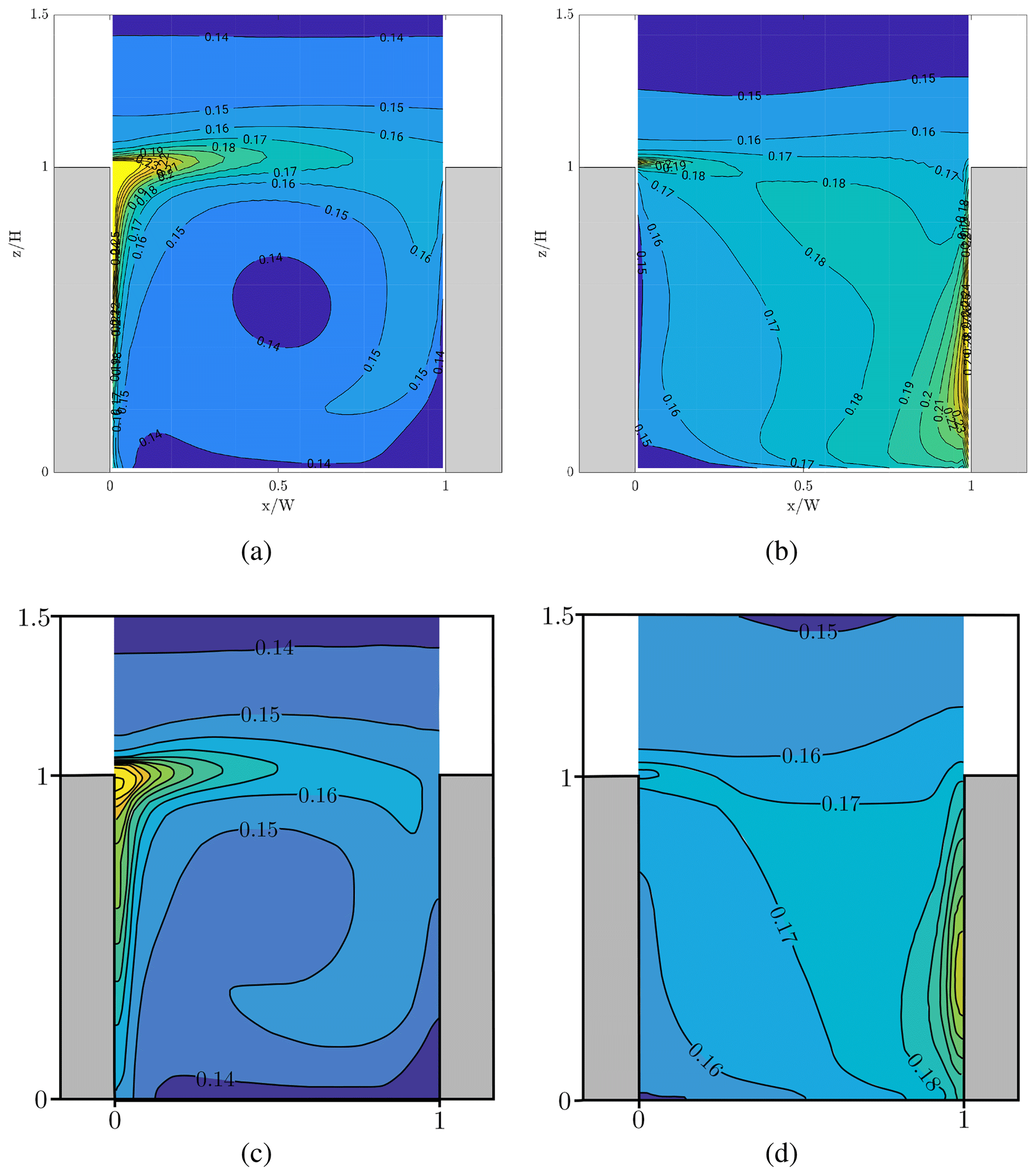
To verify the correct implementation of the wall function, results from uDALES are compared to results from a different LES model employed by Cai (2012a). The simulation set-up is a flow over a canyon-like cavity. The canyon is H=18 m high and W=18 m wide. The domain size is Lx=24 m, Ly=40 m and Lz=90 m with grid cells. This results in a resolution of Δx=0.3 m, Δy=1 m and Δz=0.3 m inside the canyon and a grid that is stretched in the vertical direction above. The simulation is periodic in x and y (Fig. 1a) and driven by a constant free-stream velocity UF=2.5 m s−1. Two cases are examined: (1) the upstream wall and roof are heated (T0+9 K, assisting case), and (2) the downstream wall and roof are heated (T0+9 K, opposing case). In Case 1 the buoyancy flux from the heated upstream wall will assist the recirculation forming inside the canyon, while in Case 2 the additional buoyancy will oppose the general flow in the cavity.
In Fig. 2 the mean temperature fields for both cases are compared to figures reproduced from Cai (2012a) and show good agreement. In the assisting case, the heat is concentrated on the upstream canyon edge from where it is efficiently mixed with air aloft. The mean temperature inside the canyon is thus only slightly elevated. In the opposing case, the downdraft along the heated wall leads to more complicated flow patterns inside the canyon, effectively reducing the exchange between the canyon and the atmosphere. As a result, more heat is trapped inside the canyon, leading to increased temperatures. The good qualitative agreement with Cai (2012a) indicates the correct implementation of the wall function for temperature for both horizontal and vertical walls.
2.5.2 Wall function for moisture
The surface moisture fluxes require additional consideration. In uDALES it is assumed that water is stored in the soil and in vegetation, with any such surface having a water balance
where W [kg m−2] is the soil moisture content, P [kg m−2 s−1] is the water supply rate, E is the latent heat flux [W m−2] and Lv [J kg−1] is the latent heat of vaporisation. The behaviour of plants under various environmental conditions has been studied extensively (Moene and van Dam, 2014). However, of major interest are the exchanges of momentum, heat and water between the surface and the atmosphere. Apart from water availability in the topsoil, the evaporation from vegetation is determined mainly by the solar radiation reaching the leaves. The phase change from liquid water into water vapour in the air requires large amounts of energy, generally provided by radiation. Furthermore, the pores in the leaves, called stomata, are open during the daytime to allow the exchange of gases used in photosynthesis, facilitating transpiration. Tall vegetation like trees also provide shade for lower surfaces. While trees are indeed a very interesting topic in the research area of the urban climate, trees and tall vegetation are not considered here.
A wall function for moisture fluxes from vegetated surfaces was newly developed for uDALES. The moisture flux from roof and wall facets can be described identically to the heat flux (Eq. 8). However, it is not obvious what the moisture difference Δq between the wall and the atmosphere is because water is usually not available directly on the surface, and therefore one cannot assume that the air close to the surface is saturated with water vapour. Furthermore, open water surfaces are as of yet uncommon on buildings, and most of the flux will thus stem from vegetation or soil of green roofs and/or walls. Plants lose water by opening their stomata but also through their outermost layer, the cuticle. A large number of processes are involved in the transport of water in soil and plants. Indeed, the nature of the ground influences the roots and their water uptake; plants have varying metabolisms depending on age, size and season, among other factors. Modelling these processes is seldom done in detail in atmospheric models. We thus utilise a modified Jarvis–Stewart (JS) approach (Jarvis, 1976; Stewart, 1988). This approach adds additional resistance to the transport of moisture from vegetation and soil to the atmosphere. The added resistance is based on empirical functions depending on plant and environmental parameters. The resistances for the plant canopy (rc, s m−1) and for the soil (rs, s m−1) can be expressed as
where D [m2 m−2] is the leaf area index, the term f1 is a function of net shortwave radiation K [W m−2], f2 depends on soil moisture content WG [kg m−3] and f3 on the wall temperature Ts [K].
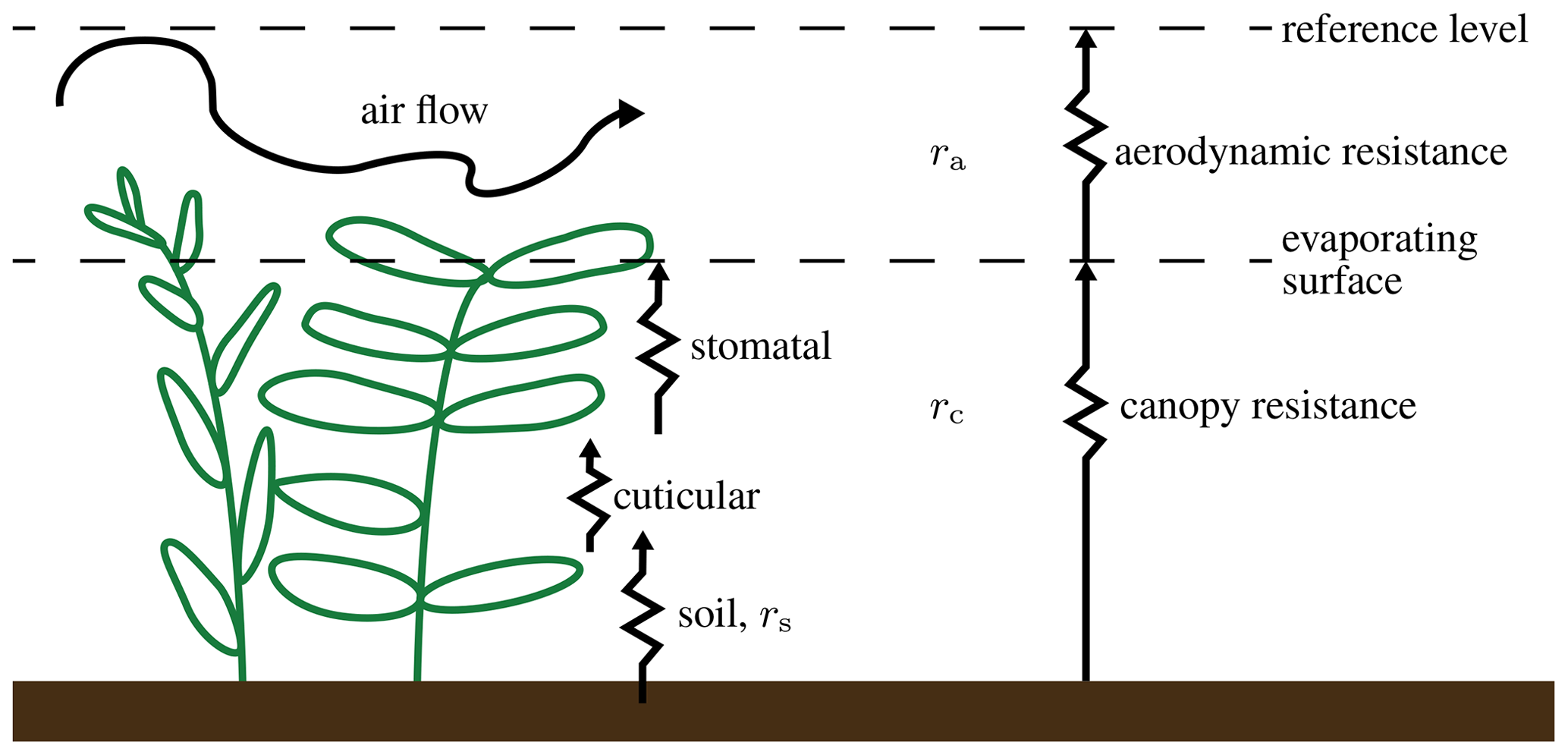
Figure 3Diagram of the resistances encountered in a simplified soil–plant–atmosphere system.
Following Van den Hurk et al. (2000) for f1 and f2 and Moene and van Dam (2014) for f3, these are given by
where c1=0.004 m2 W−1, c2=0.0016 K−2 and c3=298 K, Wwilt [kg m−3] is the soil moisture at the wilting point, Wfc [kg m−3] is the soil moisture at field capacity, and hrel [–] is the relative humidity above soil following Noilhan and Planton (1989). The moisture flux from roof and wall facets is then expressed as
with the units kg kg−1 m s−1. The heat transfer coefficient is obtained from the standard wall function (Eq. 8), wherein the vegetation is considered with appropriate roughness lengths. To determine the saturation specific humidity qsat [kg kg−1] we use empirical formulas from Bolton (1980) and Murphy and Koop (2005) that are accurate within normal temperature ranges encountered in cities.
2.6 Emissions and chemistry
A key application of urban LES models is the study of urban air pollution. This entails modelling the life cycle (emission, dispersion, chemical reaction and removal) of pollutants within the LES domain at the relevant (microclimate) scales. The high-resolution, time-resolving nature of uDALES makes it able to accurately resolve the transport of passive scalar fields within the turbulent urban flow field. The capability to model both idealised (point and line sources with initial Gaussian distributions) and realistic emissions (via networks of volumetric point sources) has been introduced into uDALES. The chemistry of the null cycle has also been added to capture the reactions between nitrogen oxides (NOx) and ozone (O3; Grylls et al., 2019).
Idealised emission sources are integral for fundamental studies of urban pollution dispersion (e.g. line sources within infinite canyons; Caton et al., 2003). Point sources are used to represent passive scalar releases in the validation of uDALES in Sect. 4.1. Realistic traffic emissions are obtained by coupling the LES model with a traffic microsimulation and emissions model within the preprocessing routine. By rasterising the resulting pollutant emissions to the grid used in uDALES, traffic emissions can be read into the LES model and simulated via a network of pollutant sources at the lowest level of the domain. Grylls et al. (2019) used the traffic microsimulation model VISSIM (PTV AG, 2017) and an instantaneous general regression emissions model (Luc Int Panis, 2006) to use uDALES to study pollution dispersion over a case study region in London, UK.
Chemical reactions occurring at a timescale similar to the dispersion of pollutants within the urban canopy layer (UCL) significantly alter the spatial and temporal evolution of the affected pollutant species. This phenomenon is particularly important in accurately capturing nitrogen dioxide (NO2) and ozone (O3) concentrations. By time-resolving the relevant reactions within urban LES, a greater understanding can be gained of these harmful air pollutants and the effect of these reactions on e.g. pedestrian-level exposure. The chemistry of the null cycle, which has no net chemical effect (meaning that NOx and Ox are conserved), follows
The photodissociation (Reaction R1) has the rate constant , and Reactions (R2) and (R3) have the first-order rate constants k2 and k3, respectively. The chemical processes of the null cycle have been added into uDALES using reaction rates from Wallace and Hobbs (2006). The relatively high reactivity of the oxygen radical, O•, permits a simplification of the null cycle, leading to the following prognostic relationships (Zhong et al., 2017):
where ϵ is an additional source term on the right-hand side of Eq. (3) for reactive pollutant fields. The chemistry is implemented following a split fully implicit time integration scheme. A validation of the chemical scheme can be found in Grylls et al. (2019).
Any attempt to understand the urban microclimate must start with an analysis of its surface energy balance (SEB; Oke et al., 2017). Urban areas exchange energy in various forms (Erell et al., 2011), such as incoming and outgoing longwave (L↓, L↑) and shortwave radiative fluxes (K↓, K↑), the turbulent sensible heat flux (H), the turbulent latent heat flux (E), ground heat flux (G), and the heat storage per unit time (, often denoted ΔQ). These fluxes have to balance, and the SEB is expressed as
where all the terms have the unit watts per square metre (W m−2).
Several possible approaches for studying the urban climate can be found in the literature: e.g. Mirzaei and Haghighat (2010), Mirzaei (2015), Moonen et al. (2012), Arnfield (2003), Rizwan et al. (2008), Grimmond (2007), and Barlow (2014). A common approach is the use of stand-alone urban energy balance (UEB) models. UEBs are based on the concept that total energy in the urban boundary layer, which is the lowest few hundred metres of the atmosphere, has to be conserved. UEBs are widely used as surface schemes in numerical weather prediction and regional atmospheric models, such as the Town Energy Budget (Masson, 2000, TEB) used by the French national weather service (Météo-France) and the Joint UK Land Environment Simulator (Best2011, Clark2011, JULES) by the UK Met Office. They include many physical processes but are a very simplified representation of the urban environment, making them computationally inexpensive. The building geometry is often only represented in an averaged sense, and no single building can be studied. Furthermore, the transport in the air is parameterised. Other UEBs include variations of TUF (Krayenhoff and Voogt, 2007; Yaghoobian and Kleissl, 2012), SUEWS (Järvi et al., 2011), RayMan (Matzarakis et al., 2010) and the SOLWEIG model (Lindberg et al., 2008). Grimmond et al. (2010) provide an overview and comparison of UEB models.
The surface energy balance in uDALES is implemented per facet, with each facet having its own material properties. All fluxes from Eqs. (20) and (9) are modelled. The surface properties WG and Ts can vary in time and are spatially heterogeneous. Often Eq. (20) is considered for a large area, averaging out many local features: e.g. in urban energy balance models the horizontal scales are usually 102–104 m (Grimmond et al., 2010). The time resolutions are correspondingly coarse. The much higher resolution of uDALES permits the consideration of individual surfaces, for which all the terms of Eq. (20) become rather intricate. The turbulent sensible and latent heat fluxes change with every wind gust, while internal wall temperatures are much less sensitive and vary on much larger timescales. Furthermore, the radiation terms depend strongly on the orientation of the surface, shading and the field of view. For example, if a large portion of the field of view of a surface is comprised of other surfaces it likely receives only little direct sunlight, since it is often shaded. However, it is likely to receive a large amount of longwave radiation from its surroundings as building walls are generally warmer than the sky.
3.1 Urban facets
uDALES accepts grid-conforming immersed boundaries (see Sect. 2.3), i.e. cuboids or blocks. These blocks therefore always span an integer number, generally more than one, of LES grid cells in each dimension. Suspended and overhanging structures are currently not supported. To represent more complex geometries, such blocks of potentially different sizes can also touch as seen in Fig. 4. For the calculation of the surface energy balance, however, it is necessary that each face (side) of a block is either entirely internal or external. For this reason, touching blocks often need to be sliced into smaller blocks. These restraints simultaneously lead to a finer representation of the surface. However, due to the grid conformity of blocks this refinement can never go below LES resolution. After all blocks have been subdivided if necessary, the outside faces are termed facets.
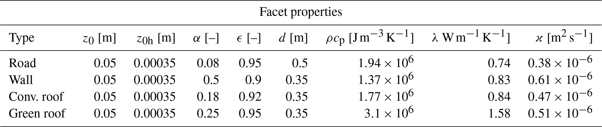
Facets represent all types of surfaces present in the urban landscape, such as roofs, walls, roads and green roofs. Every facet is thus also assigned properties accordingly. These are the momentum roughness length z0 [m], the heat roughness length z0h [m], the shortwave albedo α [–] and the longwave emissivity ϵ [–]. Furthermore, every facet consists of multiple layers, each with the properties of thickness d [m], density ρ [kg m−3], specific heat capacity cp [J kg−1 K−1] and thermal conductivity λ [W m−1 K−1]. The last three terms can be combined to form the thermal diffusivity [m2 s−1].
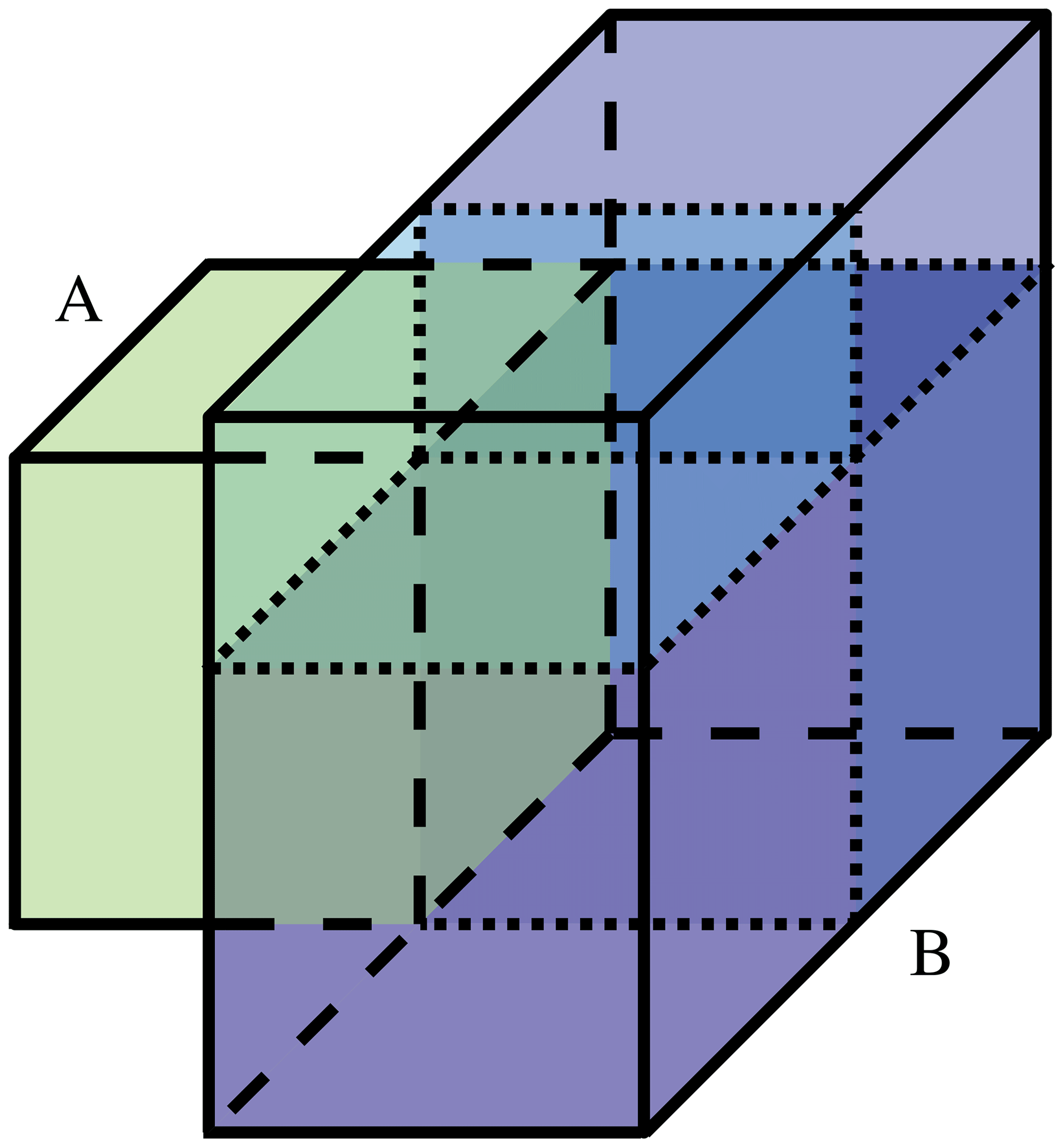
Figure 4A building consisting of two blocks A and B. Block B will be divided into four smaller blocks, so all faces are either entirely on the inside or outside of the building.
Additional facets have to be introduced to populate the voids between building blocks (i.e. roads, parks). The floor facets immediately adjoining a building are given the same length as the corresponding wall facets and a width of one grid cell. The rest of the floor is then filled with rectangles, restrained by a maximum side length. Alternatively, if the nature and configuration of the floor are known in more detail the facets can be created accordingly and be specified using the facet properties.
Following Krayenhoff and Voogt (2007) we add a wall along the domain edge of a height equal to the median building height in the domain. This wall is used to approximate the effect of the surrounding built environment on radiation that cannot be captured within the model domain. These bounding wall facets are solely used for radiative calculations and have no direct effect on airflow. An example of urban facets, including roads and bounding walls, can be seen in Fig. 11a.
3.2 View factors
To calculate the radiative exchanges between two facets, their geometric relation to one another has to be determined and the radiative processes need to be described. To achieve this, there are two alternative approaches commonly pursued in complex urban topography: (1) ray tracing and Monte Carlo simulation and (2) the radiosity approach with configuration factors. For very complex or curved surfaces radiative exchange is commonly determined by tracing randomised rays of a Monte Carlo simulation with considerable computational effort. This approach becomes more and more feasible with increasing computational power and specialised GPU computing platforms. A big advantage of this approach is its potential to also handle specular reflections. Ray tracing models have, for example, been used to study urban photovoltaic energy potential (Erdélyi et al., 2014) and urban climate and meteorology (Krayenhoff et al., 2014; Girard et al., 2017).
However, for planar surfaces, as are present in this study, the radiosity approach is generally faster (Walker et al., 2010). In this approach it is assumed that the radiosity across a facet is uniform. This allows the separation of the geometric relation between two facets from the radiative process itself (Howell et al., 2010). View factors (configuration factors) describe this geometric relation. The radiosity approach has been used to study the urban climate (e.g. Aoyagi and Takahashi, 2012; Resler et al., 2017). The approach currently employed in uDALES follows Rao and Sastri (1996). It has to be noted at this point that several conventional assumptions were made regarding the radiation and radiative properties of all of the facets (e.g. Krayenhoff et al., 2014; Howell et al., 2010), namely (1) no wavelength dependency except the separation into shortwave and longwave, (2) facets are “grey” in the longwave regime, i.e. absorptivity equals emissivity, (3) facets are isothermal, (4) reflections are diffuse, (5) emitted radiation is diffuse, and (6) the radiosity (leaving radiant flux) is uniform across the facet.
For calculating both longwave and shortwave radiation, view factors are used. The view factor ψi,j is defined as the ratio of radiation leaving the surface of facet i hitting the surface of facet j divided by the total amount of radiation leaving facet i. View factors thus take values between 0 and 1 and , where q is the set of all facets that can be seen by i (including the sky). All view factors ψi,j between any two facets i and j have to be calculated. This makes the number of calculations needed 𝒪(n2).
Several numerical methods exist to calculate view factors between surfaces, since in most cases the analytical solution to the problem is not known. The fact that view factors only depend on the geometry allows one to calculate all ψi,j a priori and store the resulting matrix as an input to the LES model. Numerical integration was used to obtain the view factors in this study. Considerable computational savings can be achieved by replacing the integration over two areas by integration over two surface boundaries. The view factor can then be expressed as (Siegel and Howell, 2001)
where S is the distance between two infinitesimal line segments along the contours of the facets (Ci,Cj). The numerical integration of ln (S) is done using sixth-order Gauss–Legendre quadrature, which is effective and accurate for straight-edged contours (Rao and Sastri, 1996). The evaluation of Eq. (21) is impossible in the case that the two contours share a common edge because S=0. Ambirajan and Venkateshan (1993) provide an exact analytical solution for the contribution from the element on the common edge of the two surfaces to the overall view factor:
where Lc is the length of the common edge. Since all facets are straight-edged, the only error in this approach lies in the approximation of ln (S) within the elemental intervals of the integration. High-order quadratures thus ensure accurate numerical results. View factors can be calculated using Eqs. (21) and (22) as long as both facets can see each other entirely. Three important exceptions can be identified: (1) the facets cannot see each other at all given their position and orientation, (2) a facet intersects the plane defined by the other facet, and (3) the view is (partly) blocked by an obstacle. The first case occurs frequently; e.g. any west-facing facet cannot possibly see any other west-facing facet or any facet that is located entirely to the east. This relationship is reciprocal. The second problem can be circumvented by cropping the intersecting facet along the intersection line. The view factors can then be calculated using the now smaller facet and the result remains accurate. There is no straightforward solution to the third problem of assessing whether the view between two facets is blocked. Depending on how the facets are arranged and the geometry of the object blocking their view, determining a precise view factor can be difficult. To avoid computationally expensive solutions we determine a percentage pb that the facets can see of each other and multiply ψ with that percentage. To obtain pb we define five points, the four corners and the centre, on every facet and determine if they can see the corresponding point on the other facet. The weight of the centre is 50 % and the weight of each corner 12.5 %.
The sky view factor (ψsky,i) denotes the fraction of radiation leaving i that enters the sky vault and does not impinge on any other facet. It is the residual view factor after summing over all facets: , where p is the total number of facets. The sky view factor is also used to determine how much diffusive radiation from the sky any facet receives. For a validation of the view factor calculations see Suter (2019).
3.3 Shortwave radiation budget
Assuming no transmission of radiation through the surface, the net shortwave radiation K (W m−2) on a facet i is defined as
where the reflected shortwave radiation (K↑) can be expressed as
The incoming shortwave radiation () can be divided into three parts (Oke et al., 2017): direct solar radiation (Si), diffuse radiation from the sky (Di) and diffusely reflected radiation from other facets (Ri).
It is important to consider all three components. Many of the urban facets can be completely shaded, thus Si=0, but potentially receive diffuse radiation from the sky or reflected radiation from other facets.
The direct solar radiation on a facet is defined as (Wu, 1995)
The solar irradiance (I) is a model input and can be a constant or follow a diurnal cycle; it is assumed that all effects of atmospheric turbidity and clouds are included. The effect of geometry is captured by the sunlit fraction of the facet fe,i, and the two cosines account for the orientation of the facet in relation to the sun. The angle υ is the solar zenith and φi the slope angle of the facet (i.e. φi=0 for a horizontal facet and for a vertical facet). The angle χi is constructed in the following way:
Here, Ωh is the solar azimuth and Ωi is the azimuth of facet i. Like the solar irradiance, the solar zenith and azimuth angles are also model inputs. Solar angles for all coordinates, dates and times can be readily obtained from online sources such as the Solar Position Calculator from the National Oceanic and Atmospheric Administration (NOAA, 2018).
The facet azimuth angles are also used to determine whether the facet is shaded or not. If is larger than , the facet is not oriented towards the sun and is thus self-shaded. If the facet i is not self-shaded the sun might still be blocked by another facet j. Therefore, the path between every non-self-shaded facet and the sun is calculated and checked if it intersects with any other facet. The same principle as for view factors is used, and the sunlit status is calculated for the four corners and the centre of the facet; the centre contributes 50 % and each corner 12.5 % to the total sunlit fraction fe,i.
The diffuse radiation (Di) is caused by light scattering in the sky and is given by
where Dsky, the total diffuse sky radiation, is a model input. The sky view factor ψsky,i is dependent on the urban geometry and has to be calculated for every facet. In Eq. (28) we ignore the directionality of Dsky, which in reality is anisotropic (Morris, 1969); this allows us to use ψsky,i directly to calculate the fraction of diffuse sky radiation impinging on i.
Shortwave radiation reflected by the environment has to be considered as well. All reflections are currently assumed to be perfectly diffusive (Lambertian); i.e. the amount of reflected light on a given surface is distributed equally in all directions. This is necessary to utilise view factors but, by definition, does not allow specular reflections. The amount of reflected light arriving at facet i is thus given by
where ψj,i is the view factor between facet j and i, and p is the total number of facets.
The calculation of the shortwave contribution is implemented into uDALES through an iterative algorithm. First, view factors for all facet pairs (i,j) are calculated and stored. The direct solar and diffuse sky radiation give an initial approximation for the shortwave budget of every facet. To account for multiple reflections, the calculation of (Eqs. 24–29) has to be iterated for all facets using the following scheme.
-
Reflection (n=0)
-
Iterate the following steps for until all changes are below a desired threshold ϵk
- 1.
only the additional reflected radiation from the previous iteration is considered for further reflections, i.e.
- 2.
recalculate Ri,n based on the updated
- 3.
update
- 4.
calculate the convergence criterion:
- 1.
Once the algorithm has converged, K↓ and also K↑ (via Eq. 24) are known for all facets. This algorithm converges quickly, usually within 10 iterations for <1 % error, since albedos are generally low, resulting in a large fraction of the radiation being absorbed and additional parts being lost towards the sky with every cycle.
3.4 Longwave radiation
The net longwave radiation L consists of four components.
where ϵi is the longwave emissivity and is the incoming longwave radiation from other facets. Since ϵi is generally close to unity for normal building materials, no reflections are considered for longwave radiation and the incoming reflected radiation . The incoming longwave radiation from the sky () is given as a model input. is the outgoing longwave radiation depending on the surface temperature Ts,i according to the Stefan–Boltzmann law with the Stefan–Boltzmann constant W m−2 K−4. The incoming longwave radiation from the other facets is given by
where p is again the total number of facets, ψj,i is the view factor between facet j and i, ϵj is the emissivity of facet j, and Ts,j is the surface temperature of facet j. The calculation of the longwave contribution thus does not require explicit iteration.
3.5 Surface energy budget of ground, wall and roof facets
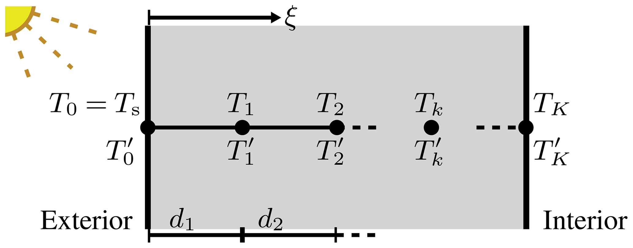
To calculate the temperature evolution of every facet, we assume that every wall and roof consist of K layers of building material (see Fig. 5). The temperature at the interface of layer and k+1 is defined as Tk. Here, is the outside surface temperature used for calculating radiation and convective heat fluxes, and ξ is the facet coordinate pointing inwards from the surface. Furthermore, is the indoor temperature of the facet, where d is the total facet thickness. At every instant, T0 is determined by the balance of energy fluxes at the surface:
The net radiation terms Ki and Li are given by the radiation calculations discussed in the previous section, and Gi is the ground heat flux (positive if heat transfers into the facet). The values of H (positive if from the facet to the atmosphere) are the time mean fluxes provided by the wall function. The net shortwave radiation Ki only depends on the position of the sun, and the incoming longwave radiation can be calculated from the other facets' surface temperatures. The two remaining unknown terms are and the ground heat flux Gi.
A defining aspect of this problem is that the boundary condition at the surface, which drives the energy exchange with the wall, is strongly non-linear. Under the assumption that the ground heat flux (Gi) is purely conductive, i.e. , the boundary condition from Eq. (32) can be written as
where and λ is the thermal conductivity in W m−1 K−1. We omit the subscript i in Eq. (33) and the description of the facet-internal processes in the rest of this section.
Equation (33) requires information about both the temperature and its gradient, and it would thus be very useful to have a numerical method for which these are both available at the same location without approximation. To achieve this, the variables are distributed in pairs of the temperature Tk and its gradient on the cell edges, implying that there are 2(K+1) unknowns if the wall is discretised into K layers. This grid layout is not conventional but is closely related to Hermitian interpolation (Peyret and Taylor, 1983) and has been used successfully to predict non-hydrostatic free-surface flow (Van Reeuwijk, 2002).
A solution will be constructed using a set of piecewise continuous quadratic polynomials, which will turn out to be splines. Consider a second-order polynomial,
valid over the interval . Defining T(ξk)=Tk, , and , it is straightforward to demonstrate that the quadratic is consistent with the following relation between the temperatures and its derivatives:
where . The coefficients a,b and c are determined by requiring that T(ξk)=Tk, and , with the result
Here, Eq. (35) was used to make the representation symmetrical in the arguments. By evaluating the temperature and its gradient at ξk and ξk+1 it becomes clear that Eq. (36) indeed satisfies the requirements of a spline, as a set of these functions produces a curve which is continuous in both the temperature and the gradient of the temperature. An important property of Eq. (36) is that the mean temperature in the layer is given by
The temperature evolution inside the wall is described by an unsteady heat equation of the form
where ϰ is the thermal diffusivity in square metres per second (m2 s−1). Integrating this equation over the interval and substituting Eq. (37) results in the relation
Equations (35) and (39) provide 2K equations. The final two equations are provided by the boundary conditions. The boundary condition at ξ=0 is of Robin type and is given by Eq. (33), where the outgoing longwave radiation is expressed in the form . At the building interior a Dirichlet boundary condition of constant temperature TK=TB is imposed.
In matrix form, the system of equations for K layers is given by
The matrix A is determined by the left-hand side and matrix B by the right-hand side of Eq. (35). The vector b contains the sum of the surface energy fluxes (without the ground heat flux and outgoing longwave radiation, i.e. ). Matrices C, D and E stem from Eq. (39) (see Suter, 2019, for more details). After rearranging and substitution of Eq. (40) into Eq. (41) we obtain
where −1 indicates matrix inversion. Note that it has been assumed here that b does not depend on time for simplicity. Time integration is done with a fully implicit backward Euler scheme. The matrices involved in this scheme are of the size (k+1)2, and matrix inversion can become expensive for walls with a large number of layers, especially considering that the calculation has to be performed for each facet individually. The pre-calculation of A−1 is possible if all facets have the same number of layers and one remaining matrix division is required for the time integration. A full validation of the scheme can be found in Suter (2019).
3.6 Surface energy and water budget of vegetated surfaces
The surface energy budget of vegetated surfaces closely follows the description in Sect. 3.5. Since no tall vegetation is considered here, vegetated surfaces can be represented by facets. The facet properties can be chosen accordingly; e.g. green roofs are often thicker than conventional roofs and vegetation albedo differs from building materials. To represent the additional roughness introduced by vegetation z0 and z0h can be adapted. In order to model a vegetated surface, a latent heat flux E is added to Eq. (32):
The values of E (positive if from the facet to the atmosphere) are the time mean fluxes provided by the wall function for moisture (see next section) and use the surface properties from the previous time step.
The soil moisture content WG,i [kg m−2] changes as water evaporates according to Eq. (9). The soil moisture budget is discretised using an explicit Euler method, which, after ensuring that , results in
where Pi [kg m−2 s−1] is a water supply rate, and ΔtE is the time interval between two energy balance time steps. We assume that all soil moisture is in the outermost layer of thickness d1,i. Furthermore, the terms for plant canopy resistances, soil resistance and relative humidity at soil level used in the wall function for moisture (Sect. 2.5.2) are adjusted based on the new values of the green roof temperature, soil moisture and radiation.
3.7 Integration into LES
A schematic of the computation order of the most relevant model routines in uDALES is shown in Fig. 6. Every time step (except the initial one) starts with applying the conditions at the lateral boundaries, e.g. periodicity. Then the effects of wet thermodynamics, such as temperature changes due to evaporating and condensing water, are considered. In the advection step, quantities are transported according to the resolved velocity field. The transport due to the non-resolved subgrid processes is calculated next, followed by additional forcings such as the Coriolis effect. Finally, the top and bottom boundary conditions are applied and the immersed boundary method ensures that there is no wind and transport into buildings. At this point the momentum, temperature and moisture fluxes from the wall functions are calculated for all surfaces based on their surfaces properties. The fluxes are then added to the prognostic Eqs. (2) and (3) before time integration is done and a new time step starts. The calculation of the energy and water budget is not done at every LES time step (t), since the timescales associated with the walls are generally much larger than the atmospheric ones. The routines to update the energy balance are thus only invoked at tE, with intervals ΔtE>Δt. The sensible and latent heat fluxes, which are calculated every calculated every LES time step, are integrated over the facets and over the ΔtE to ensure their accurate representation in the surface energy balance calculations. Since facets can extend across multiple processes, each process calculates the local wall fluxes.
If the time increment ΔtE takes q LES time increments and the facet area (A) is split across l processes (Ak), the mean latent and sensible heat fluxes on facet i are given by
At every energy balance time step tE, the longwave and shortwave budgets are updated and the water budget is calculated according to Eq. (44) using the values obtained from Eqs. (45) and (46). The new facet temperatures are calculated following Eq. (42), and subsequently the facet properties are updated accordingly. The calculation of the energy balance is done on a single processor. The information about the facet fluxes is gathered via MPI, and the updated facet properties are redistributed afterwards. The accumulation of the wall fluxes is calculated at every LES time step. However, the execution and communication time is negligible compared to the fluid dynamics calculations, which becomes obvious when comparing the number of facets 𝒪(104) to the number of fluid cells 𝒪(108).

Figure 6Schematic of the main routines in uDALES. Unshaded boxes refer to DALES core routines (see Heus et al., 2010). The grey box indicates the routines that are used when considering buildings. The green boxes refer to the energy balance routines
4.1 Validation using DAPPLE wind tunnel experiments
The dynamic core of uDALES, DALES, has been validated extensively and used as part of several atmospheric intercomparison studies (Heus et al., 2010). The adapted version of the code with the IBM implemented has been validated against both wind and water tunnel data for idealised geometries (Tomas et al., 2016; Tomas, 2016). A further validation of uDALES is presented for its application to realistic urban morphologies and passive scalar dispersion under neutral dynamic conditions using wind tunnel data from the Dispersion of Air Pollution and its Penetration into the Local Environment (DAPPLE) project.
DAPPLE was a large, multidisciplinary study of both urban meteorology and pollution dispersion that consisted of field measurements, wind tunnel modelling and computational simulations (Arnold et al., 2004). The case study area was the region surrounding the junction of Marylebone Road and Gloucester Place in central London, United Kingdom. Marylebone Road is a wide street with several lanes in each direction, aligned with building blocks of different sizes and heights. At the intersection with Gloucester Place, a street approximately half the width of Marylebone Road, is a 53 m high building on top of a wider, three-storey (11 m) base opposite a building with a 49 m tall spire. The streets in the proximity of the junction are arranged in an irregular grid-based layout.
Wind tunnel experiments with passive scalar releases were conducted over the case study region as part of the DAPPLE project (Carpentieri et al., 2009; Carpentieri and Robins, 2010; Carpentieri et al., 2012). The wind tunnel model of the study area was set up with a radius of about 500 m and at a 200:1 scale; the free-stream velocity was 2.5 m s−1, the wind direction was south-westerly and a turbulent neutral boundary layer was developed upstream of the urban geometry using Irwin spires and 2D roughness elements. The experiment contained three-dimensional velocity measurements over the Gloucester Place–Marylebone Road intersection area using laser Doppler anemometry (LDA; Carpentieri et al., 2009). Vertical velocity profiles were measured for several points in the intersection with an averaging time of 3 min. Pollution dispersion experiments were performed by releasing a tracer gas from different locations upstream of the street intersection and measuring its concentration using a fast response flame ionisation detector (FFID; Carpentieri and Robins, 2010; Carpentieri et al., 2012). Xie and Castro (2009) conducted an LES study that reproduced the wind tunnel data with good agreement.
4.1.1 Simulation set-up
A uDALES simulation is set up to reproduce the DAPPLE wind tunnel experiments, namely vertical profiles of mean (time-averaged) velocities, root mean square (rms) velocities and Reynolds shear stresses, along with a horizontal profile of mean and root mean square scalar concentrations. The target simulation uses inflow–outflow boundary conditions in the streamwise direction and is driven by a precursor simulation. Analysis of the subgrid-scale fluxes indicated that a 2 m resolution is sufficient to resolve the majority of the energetic turbulent scales with subgrid fluxes not exceeding 4.5 %, except in cells adjacent to the ground surface. Details of the two simulations are provided in Table 1. Figure 7 shows a diagrammatic view of the modelled urban morphology, which reproduces the model used in the wind tunnel experiment at full scale. The mean building height of the DAPPLE morphology, hm, is 22 m. The figure indicates the locations P1–P9 for comparison with the measured vertical velocity profiles (circles in Fig. 7), scalar release locations (triangles in Fig. 7) and the horizontal axis xs aligned with Marylebone Road along which the scalar concentrations are compared. The case study morphology is rotated such that the south-westerly incoming wind direction is aligned with the precursor simulation x direction. Additional blocks are added in the upstream area of the domain outside the study area to emulate the effects of generic buildings or roughness elements in the wind tunnel (see Xie and Castro, 2009).
Table 1Simulation set-up details for precursor and target simulations used in the uDALES validation. Boundary conditions (BCs) are defined for the x and y directions.

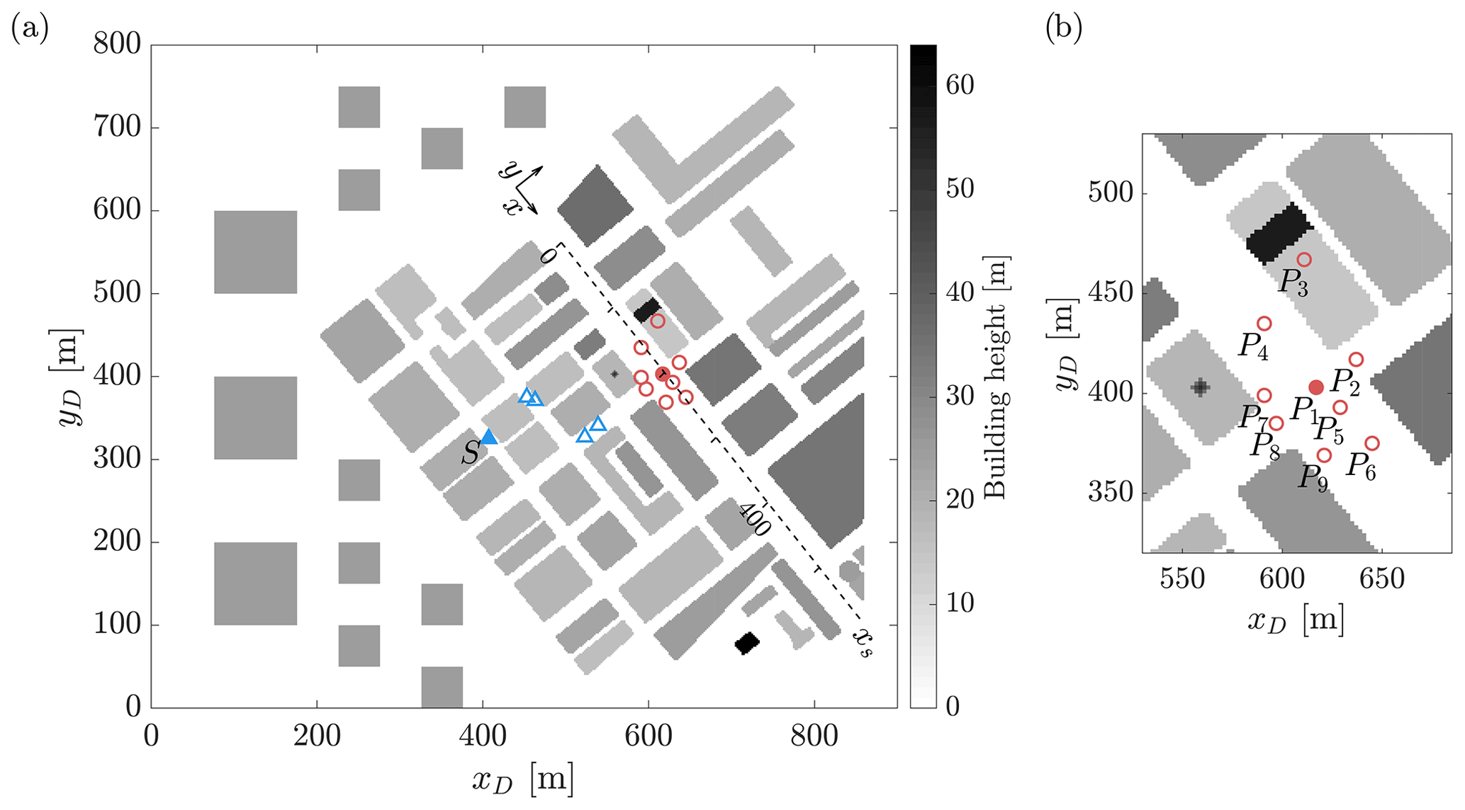
Figure 7Diagrammatic view of the (a) urban morphology in the DAPPLE simulation and (b) detailed view of the main intersection of Marylebone Road and Gloucester Place with positions of velocity profile measurements P1–P9 (circles) around the intersection and positions of the upstream scalar releases (triangles). Velocity measurements at point P1 (filled circle) and the spanwise pollutant concentration along Marylebone Road (along the horizontal axis xs) from scalar release at point S (filled triangle) are shown in Figs. 9 and 10. Additional axes x and y are aligned with Marylebone Road.
The use of a precursor simulation allows the incoming boundary layer to be defined independently of the target simulation (which can be particularly useful when reproducing wind tunnel experiments or studying transitional flows). The precursor simulation is set up to reproduce the boundary layer dynamics obtained upwind of the wind tunnel morphology in the experiment of Cheng and Robins (2004) with a free-stream velocity uref=2.5 m s−1.
A staggered cubic array was used in the precursor simulation, with a mean block height of 4 m. The height and packing density (0.25) were obtained from the mean velocity profile using the relationship defined by Macdonald et al. (1998).
Figure 8 compares the horizontally averaged mean velocity and turbulent statistics produced in the precursor simulation against the incoming profiles from the wind tunnel. Good agreement is shown, indicating that the inlet to the target simulation closely matches that of the wind tunnel data. The root mean square error between the normalised wind tunnel velocity profile and simulation velocities at corresponding heights is 0.04. The precursor simulation had to be run up to reach a statistical steady state prior to obtaining converged statistics (run-up times and averaging periods given in Table 1). The simulations were run on the UK national supercomputer ARCHER using 100 cores. The precursor simulation took 18 h and the target simulation 48 h of wall time.
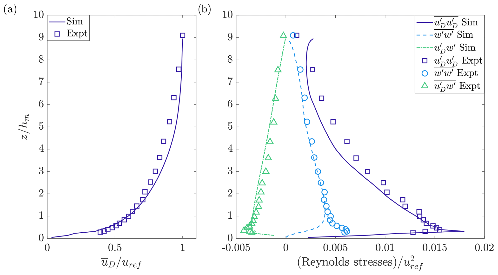
Figure 8Horizontally averaged (a) mean velocity and (b) Reynolds stress profiles of the precursor simulation and the boundary layer developed before the urban area in the wind tunnel experiments of the DAPPLE project. Note the use of subscript D to denote alignment with the axes xD and yD (see Fig. 7). The data for these profiles were averaged for 3600 s.
4.1.2 Results
Mean and turbulent flow and scalar statistics obtained in uDALES are compared to those of the wind tunnel experiments. Figure 9 compares the mean and turbulent (Reynolds stress) vertical profiles obtained at position P1 (note all variables are rotated for alignment with the axes x and y; refer to Fig. 7). Position P1 is situated within a large intersection directly downwind of an elevated spire. The simulation illustrates good agreement between all three mean velocity profiles. The second-order statistics are also shown to generally provide good agreement, with the most significant discrepancy shown to be the relatively larger peaks in the Reynolds stress profiles at z=2hm. These peaks are related to the wake of the upwind spire. Capturing the form of this spire is challenging due to its oblique angle upon the Cartesian grid (refer to Fig. 7b), and as such both its frontal area and vertical form may lead to the relatively larger fluxes over this region. Similar agreement was obtained over the eight other positions within the modelled domains.
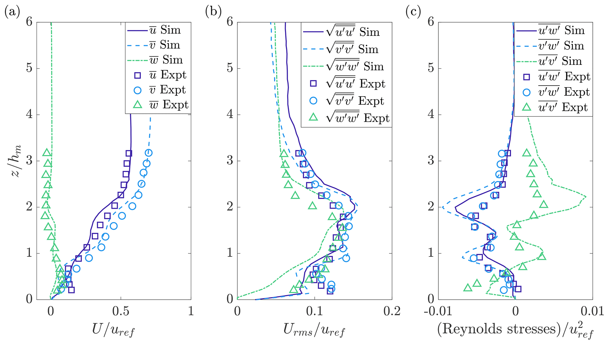
Figure 9Vertical profiles of the (a) mean velocities, (b) root mean square velocities and (c) Reynolds stresses at position P1 (see Fig. 7). Plotted against the wind tunnel experiment results of the DAPPLE project.
Table 2 displays validation metrics of the uDALES simulation with DAPPLE wind tunnel measurements for the mean velocity magnitude at measurement positions P1–P9, including the root mean square error (RMSE), fractional bias (FB) and factor of 2 (FAC2) (COST Action 732, 2007). The root mean square errors range from 0.06 to 0.15. The fractional biases are typically slightly below zero, indicating that the simulation had a small tendency to underpredict the velocities. The FAC2 measures the fraction of predictions that lie within factor of 2 of the observations, which was generally high, and for some locations all predictions (simulation velocities) are within a factor of 2 of the experiment data (i.e. FAC2 = 1).
Table 2Validation metrics of the uDALES simulation with DAPPLE wind tunnel measurements for mean velocity magnitude at positions P1–P9 and for mean scalar concentration along axis xs: the root mean square error (RMSE), fractional bias (FB) and factor of 2 (FAC2).
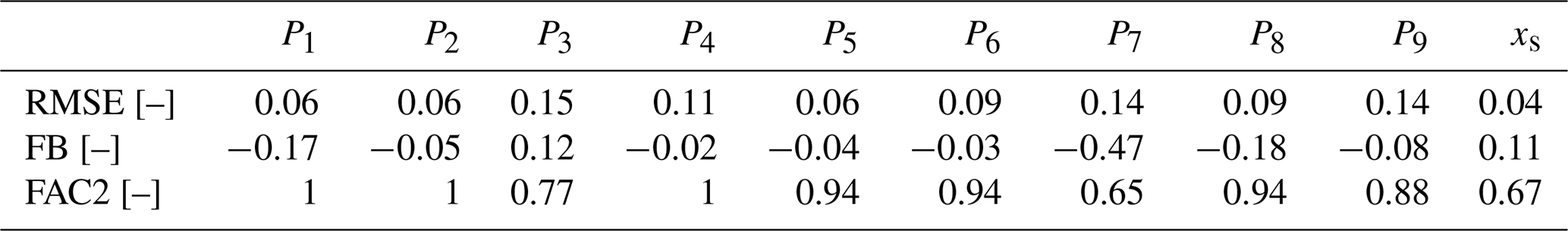
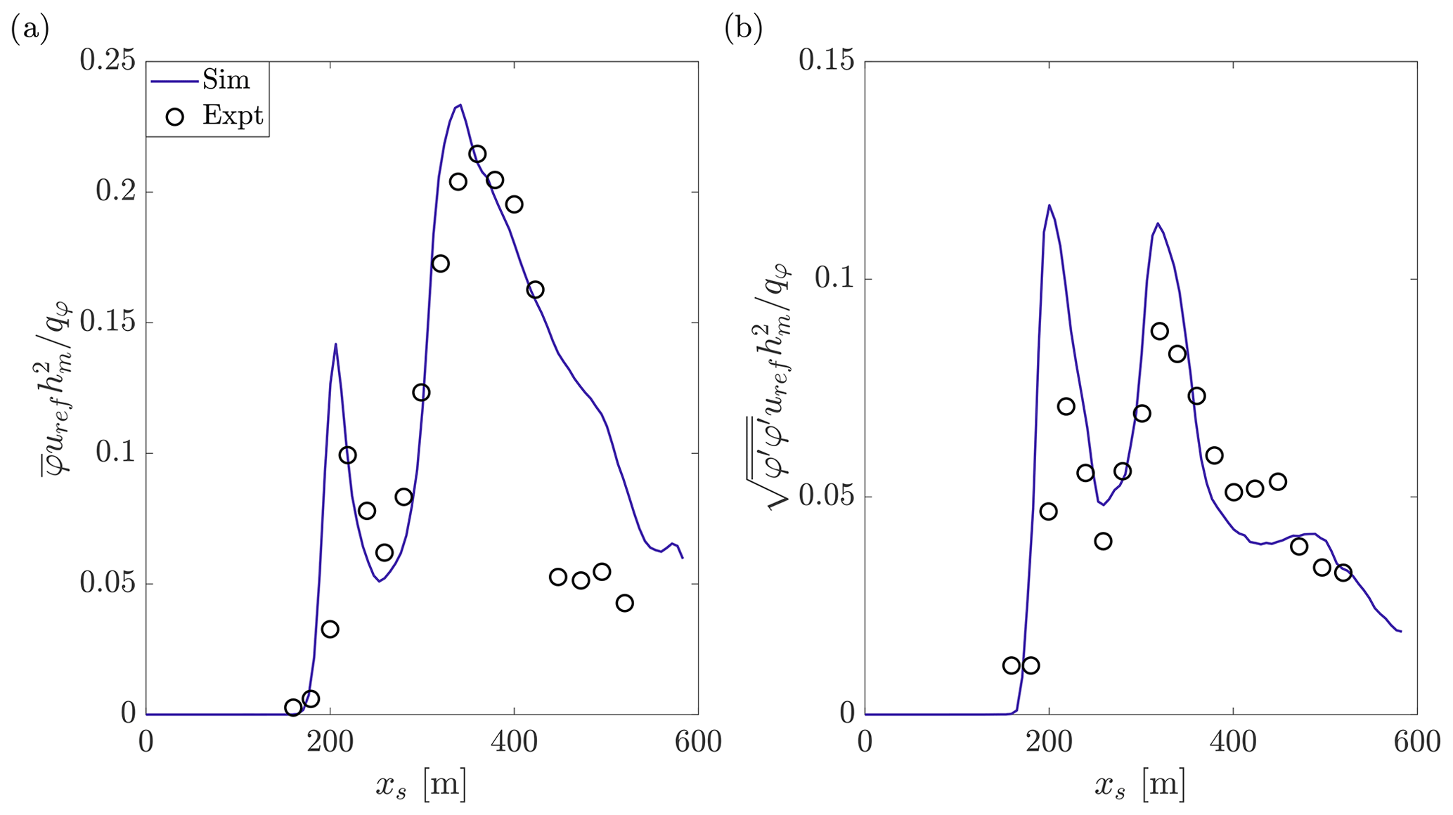
Figure 10Comparison of the normalised (a) mean scalar concentrations and (b) root mean square concentrations of the wind tunnel experiments of DAPPLE and simulation along the axis xs for a point source scalar release at position S (see Fig. 7).
Validating the model against a point source release of a passive scalar acts to validate the integrative effects of the modelled flow field (both within and above the UCL) and the treatment of scalars in the model (in particular the κ advection scheme). Figure 10 displays the mean pollutant concentration and variance along Marylebone Road (the axis xs) from a point source scalar release at position S (see Fig. 7), normalised with the reference wind speed uref, reference height hm and scalar source flux qφ (Carpentieri and Robins, 2010). The simulation is shown to provide very close agreement with the results obtained in the wind tunnel experiment in terms of both the mean concentration and the root mean square concentration. Validation metrics for the mean concentration along the axis xs are shown in Table 2. This finding validates the application of uDALES to model pollution dispersion within realistic urban morphologies.
4.2 Verification of surface energy balance
To study the behaviour of the surface energy balance in uDALES a simple case has been devised. The boundary conditions are periodic in x and y and a zero-flux boundary is imposed at the top. The layout is shown in Fig. 11a. The scenario parameters are listed in Table 3.
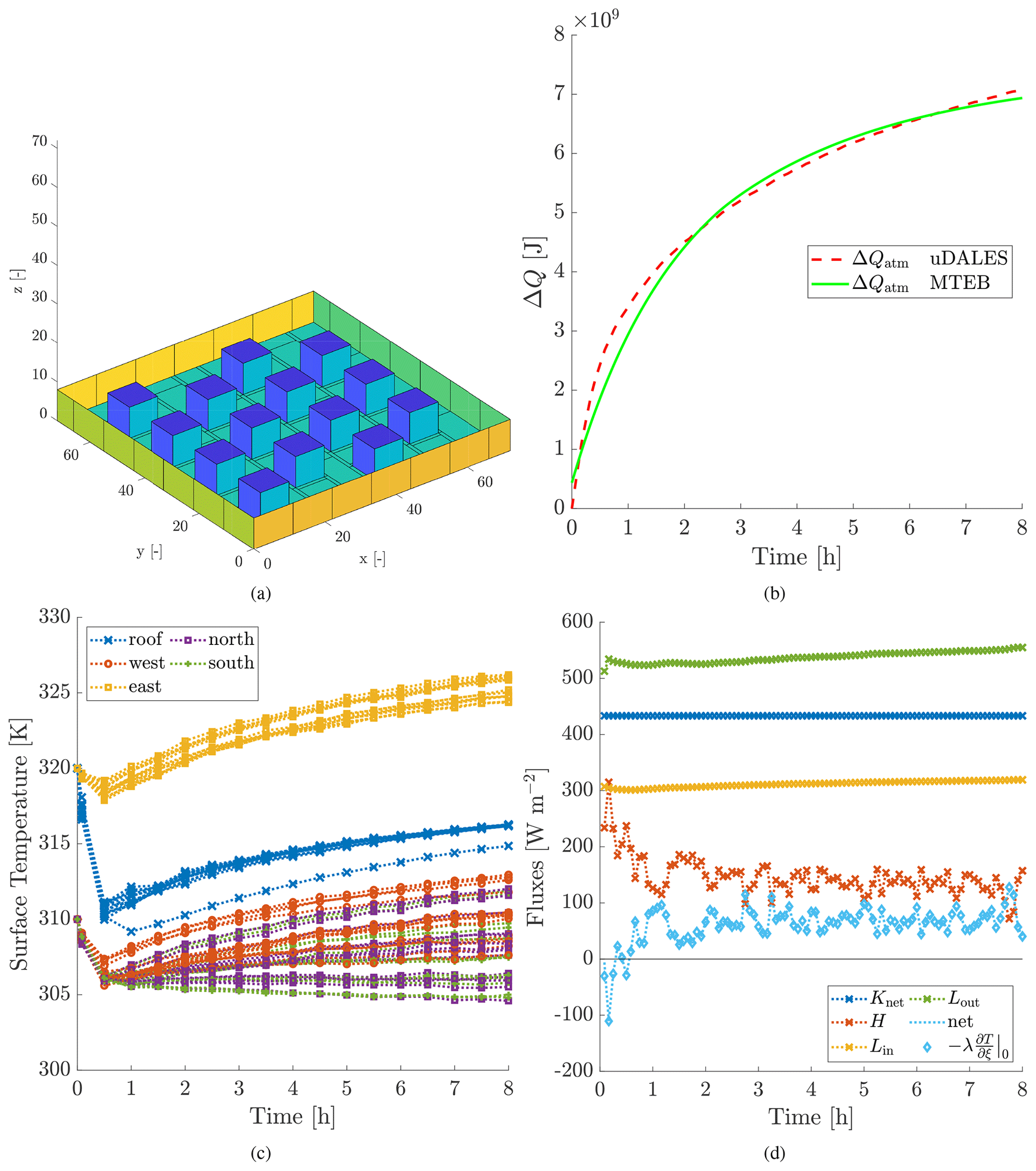
Figure 11(a) Geometry of the surface energy balance test case. (b) Comparison between uDALES and MTEB of the total energy change in the air over time. (c) Temperature evolution of all building facets. (d) Energy fluxes of a single floor facet.
The focus here is on the interaction of LES, wall function and surface energy balance. The sensible heat flux H is calculated by the wall function at every LES time step (O(1 s)) and the heat is added or removed from the fluid. This flux is integrated between energy balance time steps by using Eq. (46) with ΔtE=300 s. For the boundary conditions chosen, the temperature change of the fluid has to equal the total energy flux from the surface.
Table 3Scenario parameters of the surface energy balance test case.
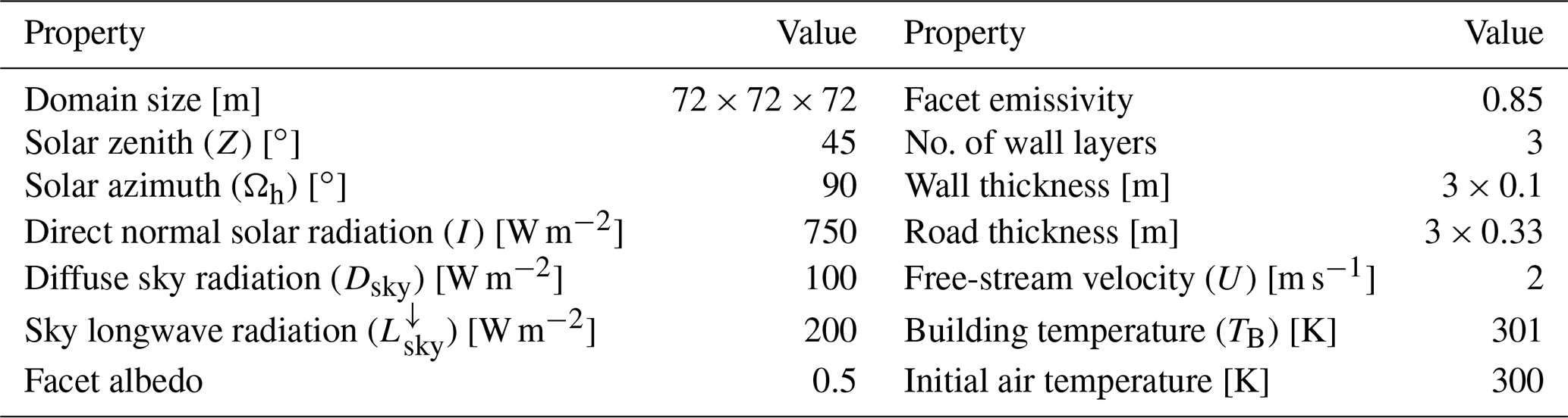
Figure 11c shows the temperature evolution of all facets. It is evident that the temperatures will be largely influenced by the solar radiation; accordingly, east-facing facets are the warmest. Furthermore, one of the roof facets was given green roof properties, resulting in lower surface temperatures, and it clearly stands apart from the other roofs.
Figure 11d shows the surface fluxes of a single road facet. Net shortwave radiation K is unchanged throughout the simulation and L only varies slightly since most facets do not experience a large surface temperature change. The sensible heat flux H shows fluctuations due to the turbulent nature of the flow. Figure 11d also demonstrates that the net flux () matches the ground heat flux () predicted by the energy balance, verifying that the energy balance is correctly linked to the wall functions.
The case presented in this section is very idealised and is thus well suited to also be studied with the urban energy balance model MTEB (Suter et al., 2017). Indeed, the geometries have been chosen to allow close correspondence between the two-dimensional MTEB and the three-dimensional uDALES. MTEB represents the urban canopy as a canyon, with the canyon orientation eliminated by integrating relevant equations horizontally over 360∘. Most of the parameters can be carried over directly. Solar and radiation properties, air temperature, and surface properties are identical to Table 3. To obtain the idealised canyon geometry in MTEB it was attempted to maintain the same morphology parameters. Considering the area covered with buildings results in a building width m. The canyon width is then given by m, and the building height remains h=8 m. The initial surface temperatures in MTEB were chosen to be the mean of the corresponding facets in uDALES. The energy balance of the entire domain is determined by the balance of the net shortwave and net longwave at the top. The effective albedo of the topography can be calculated in uDALES since the absorbed shortwave of all facets and the incoming shortwave at the top are known. Although the facets have an albedo of 0.5 the resulting effective albedo is ≈0.35 due to radiation trapping. In MTEB the resulting effective albedo is 0.37, which is in good agreement. The net longwave radiation, on the other hand, evolves during the simulations since the surface temperatures change. Figure 11b shows the total energy in the system over time for both the uDALES and MTEB runs. The canyon in MTEB does not have a heat capacity, which leads to an initial jump of energy at the start of the simulation. Over time the two curves agree well. Since the two models are completely independent this is a good indication that the surface scheme in uDALES produces plausible results.
4.3 Eastside demo
To highlight the capabilities of uDALES, this section discusses the effect that the installation of a green roof on a single building has on the local microclimate. The test area is the Imperial College campus in South Kensington, London. The green roof was installed on the Eastside building, with the motivation being that green roofs tend to be cooler than conventional roofs and can therefore improve outdoor thermal comfort on warmer days. uDALES was used to study how the flow, humidity, temperatures and surface energy balance are influenced by the presence of a green roof in comparison to a conventional roof.
The simulation domain consists of the Imperial College campus, including Eastside, as well as several other surrounding buildings. The geometry was constructed using a surface elevation map raster at 1 m resolution, obtained from GIS data. In this process, the map was rotated to broadly align with the streets, and the building heights in the simulation were set to the average of the mean and maximum heights in the GIS data. The resulting geometry is shown in Fig. 12, with the area shown in the later 3D plots highlighted in red.
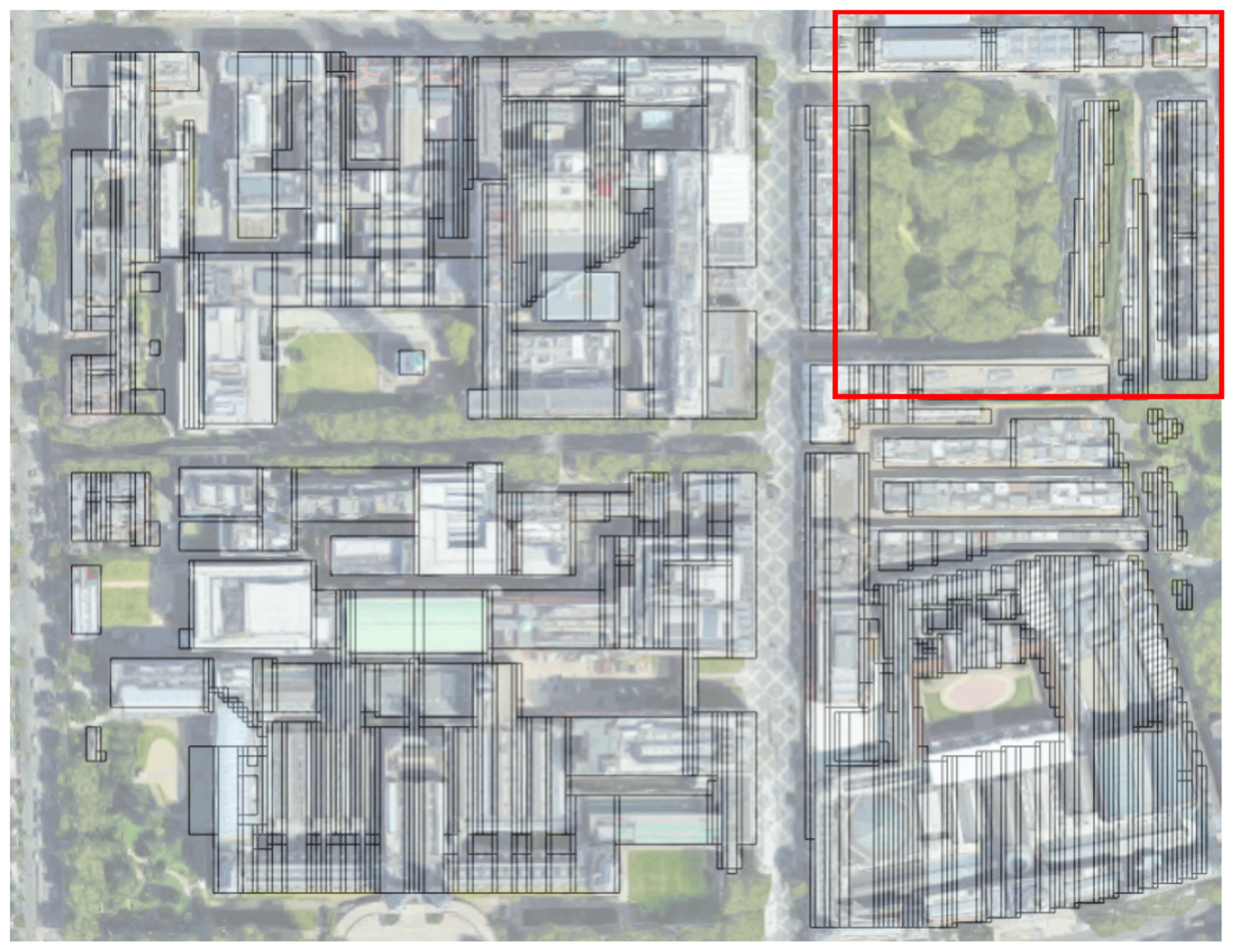
Figure 12Morphology of the South Kensington campus and surroundings divided into building blocks and overlaid over an aerial image. Imagery: © 2022 Google, © 2022 Bluesky, CNES/Airbus, Getmapping plc, Infoterra Ltd & Bluesky, Maxar Technologies, The GeoInformation Group. Map data: © 2022 Google.
The meteorological conditions were based on 21 June 2017, the hottest day in London that year. The wind was approximately easterly, so the flow is from the right of Fig. 12. The direct normal solar radiation (I) and diffuse sky radiation Dsky were determined following ASHRAE (American Society of Heating Refrigerating and Air-Conditioning Engineers Inc., 2011). Specifically, , where Z is the solar zenith, and Dsky=CI, with A=1088 W m−2, B=0.205 and C=0.134. The sky longwave was given by Swinbank's model: , where Tair is the air temperature (Swinbank, 1963). The conventional facet properties are taken from Bohnenstengel et al. (2011), and the green roof properties are taken from Oke et al. (2017). The energy balance parameters and facet properties are presented in Tables 4 and 5, respectively.
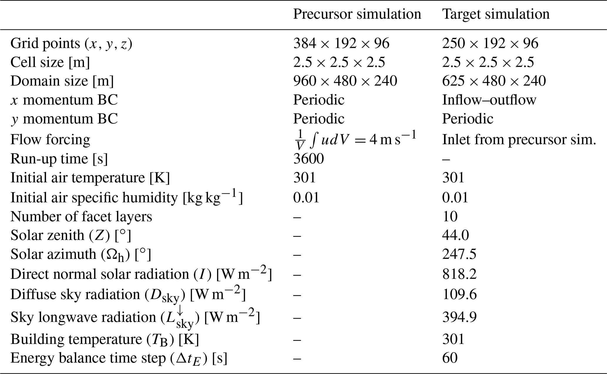
Table 5Facet properties for the Eastside demo target simulation.
Inflow–outflow boundary conditions were used, employing a precursor simulation to generate the inflow. The precursor simulation geometry consists of staggered cubes with a side length of 30 m (approximately equal to the mean building height in the target simulation) and a spacing of 10 m. This gives , which is reasonable for central London (Sützl et al., 2021a). The precursor was run for 9 h, and the outlet plane is written to file every 0.5 s starting from 1 h, thus generating 8 h of inflow data for the target simulation. The domain-averaged velocity was kept constant at U=4 m s−1. The details for the simulations are shown in Table 4. The simulations were run on ARCHER2 using 96 cores and took about 18 h of wall time.
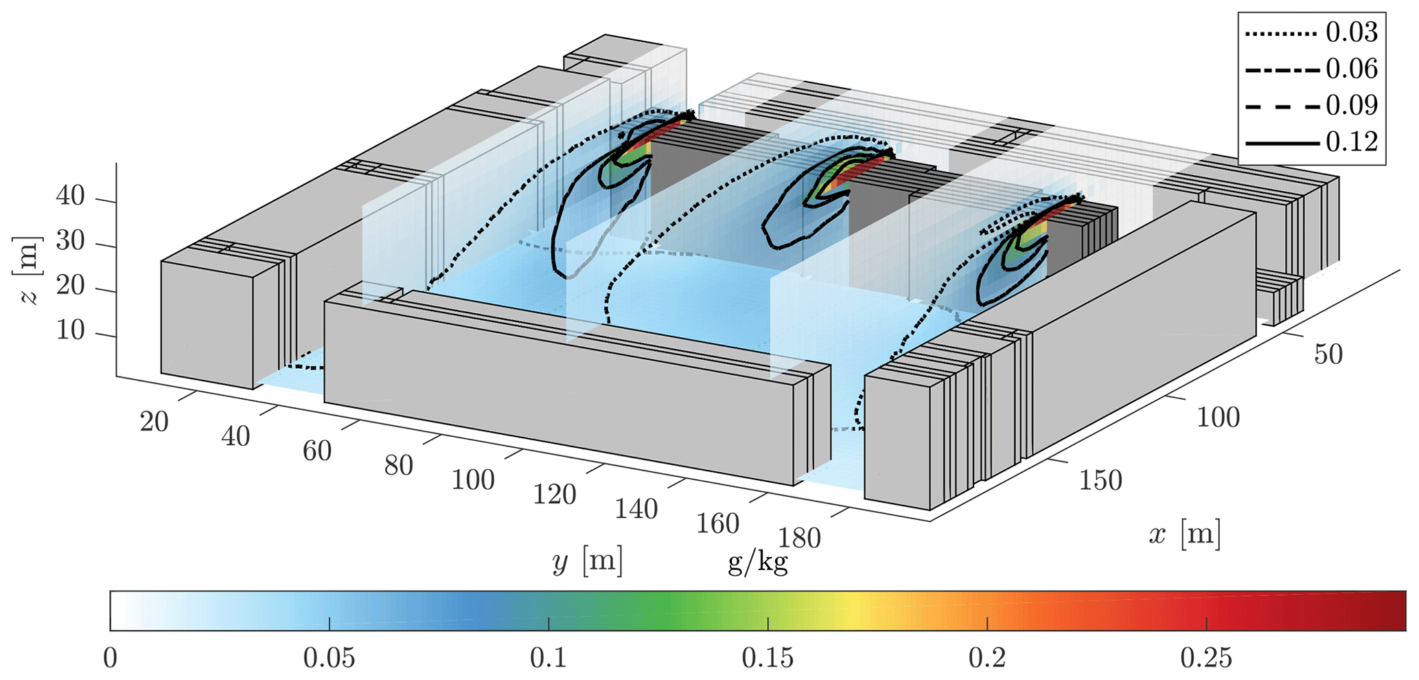
Figure 13Three vertical slices and one horizontal slice through the difference between final 1 h means of simulations with and without a green roof. The Eastside building is coloured in darker grey.
Figure 13 shows the difference between final 1 h means of the specific humidity field for simulations with and without the green roof. The green roof is a source of humidity, as expected. Clear downward mixing can be observed in the building wake. Since there is no other humidity source in the domain, the humidity difference can be attributed entirely to the presence of the green roof. On street level a mean increase in specific humidity of 0.01–0.1 g kg−1 can be observed. This corresponds to an almost insignificant difference in relative humidity, since at 301 K a relative humidity change of 1 % equals a specific humidity change of ≈0.3 g kg−1.
Figure 14 shows the facet temperatures at the end of the simulation with the green roof. Temperature maxima of up to 340 K occur in west- and south-facing walls exposed to the sun, whereas north- and east-facing facets are close to air temperature. The green roof clearly stands apart from other roofs; the temperature remains very close to the air temperature even though it is directly exposed to the sun, with a reduction of over 20 K relative to the surrounding conventional roofs. This can also be seen in Fig. 14, which compares the internal temperature profile of the Eastside roof in each case. The temperature profiles between the 11 resolved points were reconstructed following Eq. (36). Clearly, the conventional roof has absorbed much more heat in the duration of the simulation than the green roof as is evident from the much higher temperatures throughout the roof.

Figure 14(a) The Eastside building and its surrounding. Building facets are coloured based on their final surface temperature. Floors are not coloured for clarity, and grey surfaces are building-internal. View from the direction of the sun. (b) Final internal roof temperature profiles for simulations with and without a green roof on the Eastside building. The initial temperatures were 301 K throughout the roof.
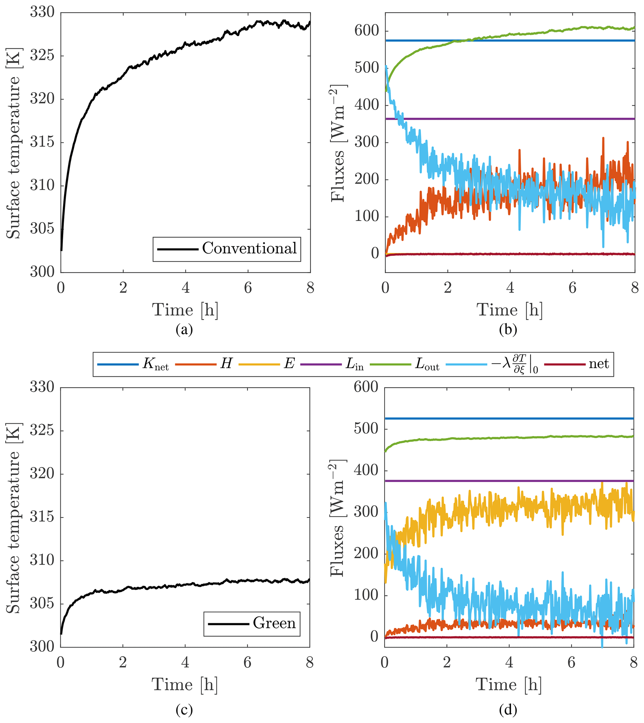
Figure 15(a) Temperature evolution of a conventional roof facet and the corresponding surface energy fluxes (b). (c) Temperature evolution of a green roof facet and the corresponding surface energy fluxes (d).
Figure 15 shows the temperature evolution and surface heat fluxes of a single facet located on the Eastside roof for both cases. The temperatures of both the conventional and green roof start at 301 K and increase over the course of the simulation. Since the incoming flow is almost identical for the conventional and green roof cases, the differences are caused mainly by the differences in facet properties. The net shortwave radiation (Knet) and the incoming longwave radiation (Lin) act to heat the surface. Knet does not change during the simulation, since the solar position does not change, and is higher for the conventional roof due to its lower albedo. There are small variations in incoming longwave radiation (Lin) due to the temperature change in surrounding facets. However, only a tiny fraction of the field of view of a roof facet on Eastside is occupied by other facets; the sky constitutes the largest part. Under the given circumstances the remaining terms act to cool the surface. The magnitude of the emitted longwave (Lout) follows the Stefan–Boltzmann law and increases along with surface temperature. The sensible heat flux (H) and latent heat flux (E) vary more substantially on short timescales due to the turbulent transport. The green roof is able to evapotranspire, resulting in a non-zero latent heat flux and comparatively less heating of the surface than the conventional roof and thus a smaller sensible heat flux. The soil moisture was kept at field capacity during the simulation, enabling the high latent heat flux. The fact that the surface is warmer than the interior results in a conductive heat flux () into the facet. Finally, the sum of these terms can be seen to be zero, which confirms that the surface energy balance is satisfied.
A new urban LES model, uDALES 1.0, was presented in this article. All model parts of uDALES were verified or validated: the wall functions (Sect. 2.5.1), scalar transport, building representation, turbulence and advection models (Sect. 4.1), and the surface energy balance (Sect. 4.2). Good agreement between uDALES and the comparison data was observed in all cases. The inclusion of explicit representation of buildings as well as energy, vegetation and chemistry processes in a high-resolution atmospheric LES model permits the study of a multitude of applications, ranging from the attribution of the urban heat island effect to various processes such as radiation trapping or heat storage in the built environment, air quality studies at very high resolutions to investigate hotspots and real-time pedestrian exposure, the effect of urban vegetation on the outdoor climate, and the energy budget of buildings. The validation and verification cases demonstrate a number of these applications of uDALES, and Sect. 4.3 demonstrates an urban climate application of uDALES in a single case.
The effect of urban trees is currently widely studied, and initial steps have been undertaken to include tall vegetation in uDALES (Grylls and van Reeuwijk, 2021). Trees can have a significant influence on pedestrian-level air quality and temperature. However, they influence a variety of processes such as radiation, latent heat and turbulence generation, which require very careful consideration. This functionality will be incorporated in the main branch of uDALES in a future release. The availability of an urban LES is ideal for the study of urban areas with reduced complexity. Indeed, the huge complexity of cities make it nearly impossible to draw general conclusions. uDALES can import idealised fractal-like urban landscapes from the Urban Landscape Generator (Sützl et al., 2021b). This tool generates urban landscapes keeping key morphological indicators such as plan- and frontal-area density constant. A systematic study of building patterns addresses the complexity gap in current urban studies between idealised building geometries and case-specific real urban geometry. The combination of uDALES and the Urban Landscape Generator was used to develop a distributed drag parameterisation (Sützl et al., 2021b), which was subsequently tested with the Met Office London Model (Sützl et al., 2021a). uDALES remains in active development; ongoing work includes an upgrade of the parallelisation to 2D by aligning uDALES with the open-source DNS code XCompact3D (Bartholomew et al., 2020) through the 2D domain decomposition library 2DECOMP&FFT (Li and Laizet, 2010).
The code of uDALES has been published and is available on Zenodo (https://doi.org/10.5281/zenodo.5111497, Grylls et al., 2021b) and GitHub https://github.com/uDALES/u-dales (last access: 28 June 2022, Suter et al., 2022). The provided model input files are for uDALES v1.0.1 (GitHub commit ID 6429fd3). We encourage contributions by other users.
All the output data and scripts to produce the relevant figures are available on Zenodo: https://doi.org/10.5281/zenodo.5480826 (Suter, 2021). The model input for the comparison with Cai (2012a, Sect. 2.5.1), the model validation (Sect. 4.1), test of the energy balance (Sect. 4.2) and the showcase (Sect. 4.3) have also been included. A general guide on how to set up the model and examples are available on the code repository.
IS authored the article and prepared tables and figures. IS initially set up and validated DALES on Imperial College infrastructure, adopted the model development by Tomas et al. (2015), and added and validated facets, wall functions, wall energy and water balances. TG extended the model with emission and nitrogen oxide–ozone chemistry capabilities, as well as inflow boundary conditions. TG, BSS and SOO conducted the comparison with DAPPLE and authored the corresponding section. SOO and CEW conducted the Eastside demo simulations. MvR acquired funding and supervised the model development. All authors edited the paper text.
The contact author has declared that neither they nor their co-authors have any competing interests.
Publisher's note: Copernicus Publications remains neutral with regard to jurisdictional claims in published maps and institutional affiliations.
The authors wish to acknowledge the support of the European Institute of Technology Climate KIC Innovation project Blue Green Dream, the EPSRC Centre for Doctoral Training in Sustainable Civil Engineering (grant reference EP/L016826/1), and the EPSRC Mathematics of Planet Earth Centre for Doctoral Training (grant reference EP/L016613/1). The computational resources for this work were provided by the Imperial College high-performance computing facilities and the national supercomputers ARCHER and ARCHER2. Resources for the latter were provided by the EPSRC-funded UK Turbulence Consortium (grant reference EP/R029326/1).
We would like to extend our gratitude to Harm Jonker and Jasper Tomas, who thoroughly introduced us to the DALES model, and to David Meyer for his contribution to making the code open-source and professionalising the workflow. Furthermore, we would like to thank Alan Robins and Zheng-Tong Xie for providing the DAPPLE wind tunnel data and geometry. Maarten van Reeuwijk is grateful to Cedo Maksimovic for enthusing him to work on urban fluid mechanics problems.
This research has been supported by the Engineering and Physical Sciences Research Council (grant nos. EP/L016826/1, EP/L016613/1, and EP/R029326/1).
This paper was edited by Leena Järvi and reviewed by two anonymous referees.
Ambirajan, A. and Venkateshan, S. P.: Accurate determination of diffuse view factors between planar surfaces, Int. J. Heat Mass Transf., 36, 2203–2208, https://doi.org/10.1016/S0017-9310(05)80151-6, 1993. a
American Society of Civil Engineers Task Committee on Outdoor Human Comfort ASCE: Outdoor human comfort and its assessment: state of the art, American Society of Civil Engineers (ASCE), Reston, VA, 68 pp., ISBN 0784406847, 2004. a
American Society of Civil Engineers Task Committee on Urban Aerodynamics ASCE: Urban aerodynamics: wind engineering for urban planners and designers, American Society of Civil Engineers (ASCE), Reston, VA, 63 pp., ISBN 9780784411797, 2011. a
American Society of Heating Refrigerating and Air-Conditioning Engineers Inc. (ASHRAE): 2011 ASHRAE Handbook: Heating, Ventilating, and Air-Conditioning Applications, chapter 35, Solar energy use, American Society of Heating, Refrigerating and Air-Conditioning Engineers, Inc., 1108 pp., ISBN 978-1-936504-07-7, 2011. a
Aoyagi, T. and Takahashi, S.: Development of an Urban Multilayer Radiation Scheme and Its Application to the Urban Surface Warming Potential, Bound.-Lay. Meteorol., 142, 305–328, https://doi.org/10.1007/s10546-011-9679-0, 2012. a
Arakawa, A. and Lamb, V. R.: Computational design of the basic dynamical processes of the UCLA general circulation model, in: Methods Comput. Phys., edited by: Chang, J., vol. 17, Academic Press, New York, NY, USA, pp. 173–265, https://doi.org/10.1016/B978-0-12-460817-7.50009-4, 1977. a
Arnfield, A. J.: Two decades of urban climate research: A review of turbulence, exchanges of energy and water, and the urban heat island, Int. J. Climatol., 23, 1–26, https://doi.org/10.1002/joc.859, 2003. a
Arnold, S., ApSimon, H., Barlow, J. F., Belcher, S. E., Bell, M., Boddy, J., Britter, R., Cheng, H., Clark, R., and Colvile, R.: Introduction to the DAPPLE Air Pollution Project, Sci. Total Environ., 332, 139–153, https://doi.org/10.1016/j.scitotenv.2004.04.020, 2004. a
Barlow, J. F.: Progress in observing and modelling the urban boundary layer, Urban Clim., 10, 216–240, https://doi.org/10.1016/j.uclim.2014.03.011, 2014. a, b
Bartholomew, P., Deskos, G., Frantz, R. A., Schuch, F. N., Lamballais, E., and Laizet, S.: Xcompact3D: An open-source framework for solving turbulence problems on a Cartesian mesh, SoftwareX, 12, 100550, https://doi.org/10.1016/j.softx.2020.100550, 2020. a
Blocken, B.: Computational Fluid Dynamics for urban physics: Importance, scales, possibilities, limitations and ten tips and tricks towards accurate and reliable simulations, Build. Environ., 91, 219–245, https://doi.org/10.1016/j.buildenv.2015.02.015, 2015. a, b
Blocken, B., Roels, S., and Carmeliet, J.: A numerical study of wind nuisance for a high-rise building group, in: Proceedings of the 2nd International conference on Research in Building Physics, Leuven, Belgium, 14–18 September 2003, edited by: Carmeliet, J., Hens, H., and Vermeir, G., pp. 981–990, https://doi.org/10.1201/9781003078852, 2003. a
Blocken, B., Stathopoulos, T., and van Beeck, J.: Pedestrian-level wind conditions around buildings: Review of wind-tunnel and CFD techniques and their accuracy for wind comfort assessment, Build. Environ., 100, 50–81, https://doi.org/10.1016/j.buildenv.2016.02.004, 2016. a
Bohnenstengel, S., Evans, S., Clark, P. A., and Belcher, S.: Simulations of the London urban heat island, Q. J. Roy. Meteor. Soc., 137, 1625–1640, 2011. a
Bolton, D.: The computation of equivalent potential temperature, Mon. Weather Rev., 108, 1046–1053, https://doi.org/10.1175/1520-0493(1980)108<1046:TCOEPT>2.0.CO;2, 1980. a
Borge, R., Santiago, J. L., de la Paz, D., Martín, F., Domingo, J., Valdés, C., Sánchez, B., Rivas, E., Rozas, M. T., Lázaro, S., Pérez, J., and Fernández, Á.: Application of a short term air quality action plan in Madrid (Spain) under a high-pollution episode-Part II: Assessment from multi-scale modelling, Sci. Total Environ., 635, 1574–1584, https://doi.org/10.1016/j.scitotenv.2018.04.323, 2018. a
Bozovic, R., Maksimovic, C., Mijic, A., Smith, K., Suter, I., and Van Reeuwijk, M.: Blue Green Solutions. A Systems Approach to Sustainable and Cost-effective Urban Development, Tech. Rep., Imperial College London, https://doi.org/10.13140/RG.2.2.30628.07046, 2017. a
Cai, X.-M.: Effects of Wall Heating on Flow Characteristics in a Street Canyon, Bound.-Lay. Meteorol., 142, 443–467, https://doi.org/10.1007/s10546-011-9681-6, 2012a. a, b, c, d, e, f
Cai, X.-M.: Effects of differential wall heating in street canyons on dispersion and ventilation characteristics of a passive scalar, Atmos. Environ., 51, 268–277, https://doi.org/10.1016/j.atmosenv.2012.01.010, 2012b. a
Carpentieri, M. and Robins, A. G.: Tracer Flux Balance at an Urban Canyon Intersection, Bound.-Lay. Meteorol., 135, 229–242, https://doi.org/10.1007/s10546-010-9471-6, 2010. a, b, c
Carpentieri, M., Robins, A. G., and Baldi, S.: Three-Dimensional Mapping of Air Flow at an Urban Canyon Intersection, Bound.-Lay. Meteorol., 133, 277–296, https://doi.org/10.1007/s10546-009-9425-z, 2009. a, b
Carpentieri, M., Hayden, P., and Robins, A. G.: Wind tunnel measurements of pollutant turbulent fluxes in urban intersections, Atmos. Environ., 46, 669–674, https://doi.org/10.1016/j.atmosenv.2011.09.083, 2012. a, b
Castleton, H. F., Stovin, V., Beck, S. B. M., and Davison, J. B.: Green roofs; building energy savings and the potential for retrofit, Energy Build., 42, 1582–1591, https://doi.org/10.1016/j.enbuild.2010.05.004, 2010. a
Caton, F., Britter, R. E., and Dalziel, S.: Dispersion mechanisms in a street canyon, Atmos. Environ., 37, 693–702, https://doi.org/10.1016/S1352-2310(02)00830-0, 2003. a, b
Cheng, H. and Robins, A. G.: Wind tunnel simulation of field tracer release in London, in: Fourth International Conference on Fluid Mechanics, Dalian, China, 28–31 July 2004, 2004. a
COST Action 732: Model evaluation guidance and protocol document, edited by: Britter, R. E. and Schatzmann, M., Tech. Rep., University of Hamburg, 28 pp., ISBN 3-00-018312-4, https://mi-pub.cen.uni-hamburg.de/fileadmin/files/forschung/techmet/cost/cost_732/pdf/GUIDANCE_AND_PROTOCOL_DOCUMENT_1-5-2007_www.pdf (last access: 8 June 2022), 2007. a
Ehrhard, J., Khatib, I. A., Winkler, C., Kunz, R., Moussiopoulos, N., and Ernst, G.: The microscale model MIMO: development and assessment, J. Wind Eng. Ind. Aerodyn., 85, 163–176, https://doi.org/10.1016/S0167-6105(99)00137-3, 2000. a
Emanuel, K. A.: Atmospheric convection, Oxford University Press on Demand, ISBN 9780195066302, 1994. a
Erdélyi, R., Wang, Y., Guo, W., Hanna, E., and Colantuono, G.: Three-dimensional SOlar RAdiation Model (SORAM) and its application to 3-D urban planning, Sol. Energy, 101, 63–73, https://doi.org/10.1016/j.solener.2013.12.023, 2014. a
Erell, E., Pearlmutter, D., and Williamson, T.: Urban microclimate – Designing the spaces between buildings, 1st edn., Routledge, ISBN 9781844074679, 2011. a
Garratt, J. R.: The atmospheric boundary layer, 1st edn., Cambridge Univeristy Press, 316 pp., ISBN 0521380529, 1992. a
Girard, P., Nadeau, D. F., Pardyjak, E. R., Overby, M., Willemsen, P., Stoll, R., Bailey, B. N., and Parlange, M. B.: Evaluation of the QUIC-URB wind solver and QESRadiant radiation-transfer model using a dense array of urban meteorological observations, Urban Clim., 24, 657–674, https://doi.org/10.1016/j.uclim.2017.08.006, 2017. a
Grimmond, C. S. B., Blackett, M., Best, M. J., Barlow, J., Baik, J. J., Belcher, S. E., and Bohnenstengel, S. I.: The International Urban Energy Balance Models Comparison Project: First Results from Phase 1, J. Appl. Meteor. Clim., 49, 1268–1292, https://doi.org/10.1175/2010JAMC2354.1, 2010. a, b
Grimmond, S.: Urbanization and global environmental change: local effects of urban warming, Geogr. J., 173, 83–88, https://doi.org/10.1111/j.1475-4959.2007.232_3.x, 2007. a
Grylls, T.: Simulating air pollution in the urban microclimate, PhD thesis, Imperial College London, https://doi.org/10.25560/91884, 2020. a
Grylls, T. and van Reeuwijk, M.: Tree model with drag, transpiration, shading and deposition: Identification of cooling regimes and large-eddy simulation, Agr. Forest Meteorol., 298–299, 108288, https://doi.org/10.1016/j.agrformet.2020.108288, 2021. a
Grylls, T., Le Cornec, C. M., Salizzoni, P., Soulhac, L., Stettler, M. E., and van Reeuwijk, M.: Evaluation of an operational air quality model using large-eddy simulation, Atmos. Environ. X, 3, 100041, https://doi.org/10.1016/j.aeaoa.2019.100041, 2019. a, b, c, d
Grylls, T., Suter, I., Sützl, B., Owens, S., Meyer, D., and van Reeuwijk, M.: uDALES: large-eddy-simulation software for urban flow, dispersion, and microclimate modelling, J. Open Source Softw., 6, 3055, https://doi.org/10.21105/joss.03055, 2021a. a
Grylls, T., Suter, I., Sützl, B., Owens, S., Meyer, D., and van Reeuwijk, M.: uDALES: large-eddy-simulation software for urban flow, dispersion, and microclimate modelling (v1.0.0), Zenodo [code], https://doi.org/10.5281/zenodo.5111497, 2021b. a
Hanjalić, K. and Kenjereš, S.: Some developments in turbulence modeling for wind and environmental engineering, J. Wind Eng. Ind. Aerod., 96, 1537–1570, 2008. a
Heus, T., van Heerwaarden, C. C., Jonker, H. J. J., Pier Siebesma, A., Axelsen, S., van den Dries, K., Geoffroy, O., Moene, A. F., Pino, D., de Roode, S. R., and Vilà-Guerau de Arellano, J.: Formulation of the Dutch Atmospheric Large-Eddy Simulation (DALES) and overview of its applications, Geosci. Model Dev., 3, 415–444, https://doi.org/10.5194/gmd-3-415-2010, 2010. a, b, c, d, e, f
Hölling, M. and Herwig, H.: Asymptotic analysis of the near-wall region of turbulent natural convection flows, J. Fluid Mech., 541, 383–397, https://doi.org/10.1017/S0022112005006300, 2005. a
Howell, J. R., Menguc, M. P., and Siegel, R.: Thermal radiation heat transfer, 5th edn., CRC press, ISBN 1439894558, 2010. a, b
Hundsdorfer, W., Koren, B., vanLoon, M., and Verwer, J. G.: A positive finite-difference advection scheme, J. Comput. Phys., 117, 35–46, https://doi.org/10.1006/jcph.1995.1042, 1995. a
Huttner, S.: Further development and application of the 3D microclimate simulation ENVI-met, PhD thesis, Johannes Gutenberg-Universität Mainz, https://doi.org/10.25358/openscience-2022, 2012. a
Isymov, N. and Davenport, A. G.: The ground level wind environment in built up areas, in: Proceedings of the 4th International Conference on Wind Effects on Buildings and Structures, edited by: Eaton, K. J., Heathrow, 1975, pp. 403–422, Cambridge University Press, ISBN 9780521208017, 1975. a
Järvi, L., Grimmond, C. S. B., and Christen, A.: The surface urban energy and water balance scheme (SUEWS): Evaluation in Los Angeles and Vancouver, J. Hydrol., 411, 219–237, https://doi.org/10.1016/j.jhydrol.2011.10.001, 2011. a
Jarvis, P. G.: The Interpretation of the Variations in Leaf Water Potential and Stomatal Conductance Found in Canopies in the Field, Philos. Trans. R. Soc. London B Biol. Sci., 273, 593–610, https://doi.org/10.1098/rstb.1976.0035, 1976. a
Kong, H., Choi, H., and Lee, J. S.: Direct numerical simulation of turbulent thermal boundary layers, Phys. Fluids, 12, 2555–2568, https://doi.org/10.1063/1.1287912, 2000. a
Kotthaus, S. and Grimmond, C. S. B.: Atmospheric boundary-layer characteristics from ceilometer measurements. Part 2: Application to London's urban boundary layer, Q. J. Roy. Meteorol. Soc., 144, 1511–1524, 2018. a
Krayenhoff, E. S. and Voogt, J.: A microscale three-dimensional urban energy balance model for studying surface temperatures, Bound.-Lay. Meteorol., 123, 433–461, https://doi.org/10.1007/s10546-006-9153-6, 2007. a, b
Krayenhoff, E. S., Christen, A., Martilli, A., and Oke, T. R.: A Multi-layer Radiation Model for Urban Neighbourhoods with Trees, Bound.-Lay. Meteorol., 151, 139–178, https://doi.org/10.1007/s10546-013-9883-1, 2014. a, b
Lawson, T. V. and Penwarden, A. D.: The effect of wind on people in the vicinity of buildings, in: Proceedings of the 4th International Conference on Wind Effects on Buildings and Structures, Heathrow, 1975, edited by: Eaton, K. J., Cambridge University Press, ISBN 9780521208017, 1975. a
Lelieveld, J., Evans, J. S., Fnais, M., Giannadaki, D., and Pozzer, A.: The contribution of outdoor air pollution sources to premature mortality on a global scale, Nature, 525, 367–371, https://doi.org/10.1038/nature15371, 2015. a, b
Li, N. and Laizet, S.: 2DECOMP&FFT – A Highly Scalable 2D Decomposition Library and FFT Interface, https://www.turbulencesimulation.com/uploads/5/8/7/2/58724623/2010_laizet_nag.pdf (last access: 8 June 2022), 2010. a
Lindberg, F., Holmer, B., and Thorsson, S.: SOLWEIG 1.0 – Modelling spatial variations of 3D radiant fluxes and mean radiant temperature in complex urban settings, Int. J. Biometeorol., 52, 697–713, https://doi.org/10.1007/s00484-008-0162-7, 2008. a
Llaguno-Munitxa, M. and Bou-Zeid, E.: Shaping buildings to promote street ventilation: A large-eddy simulation study, Urban Clim., 26, 76–94, 2018. a
Luc Int Panis, Steven Broekx, R. L.: Modelling instantaneous traffic emission and the influence of traffic speed limits, Sci. Total Environ., 371, 270–285, 2006. a
Macdonald, R. W., Griffiths, R. F., and Hall, D. J.: An improved method for the estimation of surface roughness of obstacle arrays, Atmos. Environ., 32, 1857–1864, https://doi.org/10.1016/S1352-2310(97)00403-2, 1998. a
Maronga, B., Banzhaf, S., Burmeister, C., Esch, T., Forkel, R., Fröhlich, D., Fuka, V., Gehrke, K. F., Geletič, J., Giersch, S., Gronemeier, T., Groß, G., Heldens, W., Hellsten, A., Hoffmann, F., Inagaki, A., Kadasch, E., Kanani-Sühring, F., Ketelsen, K., Khan, B. A., Knigge, C., Knoop, H., Krč, P., Kurppa, M., Maamari, H., Matzarakis, A., Mauder, M., Pallasch, M., Pavlik, D., Pfafferott, J., Resler, J., Rissmann, S., Russo, E., Salim, M., Schrempf, M., Schwenkel, J., Seckmeyer, G., Schubert, S., Sühring, M., von Tils, R., Vollmer, L., Ward, S., Witha, B., Wurps, H., Zeidler, J., and Raasch, S.: Overview of the PALM model system 6.0, Geosci. Model Dev., 13, 1335–1372, https://doi.org/10.5194/gmd-13-1335-2020, 2020. a
Masson, V.: A physically-based scheme for the urban energy budget in atmospheric models, Bound.-Lay. Meteorol., 94, 357–397, https://doi.org/10.1023/A:1002463829265, 2000. a
Matzarakis, A., Rutz, F., and Mayer, H.: Modelling radiation fluxes in simple and complex environments: basics of the RayMan model, Int. J. Biometeorol., 54, 131–139, https://doi.org/10.1007/s00484-006-0061-8, 2010. a
Mirzaei, P. A.: Recent challenges in modeling of urban heat island, Sustain. Cities Soc., 19, 200–206, https://doi.org/10.1016/j.scs.2015.04.001, 2015. a
Mirzaei, P. A. and Haghighat, F.: Approaches to study urban heat island – abilities and limitations, Build. Environ., 45, 2192–2201, 2010. a
Mittal, R. and Iaccarino, G.: Immersed Boundary Methods, Annu. Rev. Fluid Mech., 37, 239–261, https://doi.org/10.1146/annurev.fluid.37.061903.175743, 2005. a
Moene, A. F. and van Dam, J. C.: Transport in the atmosphere-vegetation-soil continuum, 1st edn., Cambridge University Press, ISBN 0521195683, 2014. a, b
Monin, A. S. and Obukhov, A. M.: Basic laws of turbulent mixing in the surface layer of the atmosphere, Contrib. Geophys. Inst. Acad. Sci. USSR, 24, 163–187, 1954. a
Moonen, P., Defraeye, T., Dorer, V., Blocken, B., and Carmeliet, J.: Urban Physics: Effect of the micro-climate on comfort, health and energy demand, Front. Archit. Res., 1, 197–228, https://doi.org/10.1016/j.foar.2012.05.002, 2012. a
Morris, C. W.: The anisotropy of diffuse solar radiation, PhD thesis, Texas Tech University, http://hdl.handle.net/2346/9001 (last access: 8 June 2022), 1969. a
Murphy, D. M. and Koop, T.: Review of the vapour pressures of ice and supercooled water for atmospheric applications, Q. J. Roy. Meteor. Soc., 131, 1539–1565, https://doi.org/10.1256/qj.04.94, 2005. a
Musy, M., Malys, L., Morille, B., and Inard, C.: The use of SOLENE-microclimat model to assess adaptation strategies at the district scale, Urban Clim., 14, 213–223, https://doi.org/10.1016/j.uclim.2015.07.004, 2015. a
NOAA: Solar Position Calculator, https://www.esrl.noaa.gov/gmd/grad/solcalc/azel.html (last access: 8 June 2022), 2018. a
Noilhan, J. and Planton, S.: A Simple Parameterization of Land Surface Processes for Meteorological Models, Mon. Weather Rev., 117, 536–549, https://doi.org/10.1175/1520-0493(1989)117<0536:ASPOLS>2.0.CO;2, 1989. a
Obukhov, A. M.: Turbulence in an atmosphere with inhomogeneous temperature, Tr, Inst. Teor. Geofis. Akad. Nauk. SSSR, 1, 95–115, 1946. a
Oke, T. R.: The energetic basis of the urban heat island, Q. J. Roy. Meteor. Soc., 108, 1–24, https://doi.org/10.1002/qj.49710845502, 1982. a
Oke, T. R., Mills, G., Christen, A., and Voogt, J. A.: Urban Climates, 1st edn., Cambridge University Press, ISBN 9780521849500, https://doi.org/10.1017/9781139016476, 2017. a, b, c, d
Peyret, R. and Taylor, T. D.: Computational methods for fluid flow, 1st edn., Springer Science & Business Media, 358 pp., ISBN 9783642859526, https://doi.org/10.1007/978-3-642-85952-6, 1983. a
Pourquie, M., Breugem, W. P., and Boersma, B. J.: Some Issues Related to the Use of Immersed Boundary Methods to Represent Square Obstacles, Int. J. Multiscale Comput. Eng., 7, 509–522, https://doi.org/10.1615/IntJMultCompEng.v7.i6.30, 2009. a
PTV AG: PTV VISSIM 9 User Manual, PTV AG, 1084 pp., https://www.myptv.com/en/mobility-software/ptv-vissim (last access: 8 June 2022), 2017. a
Pyrgou, A. and Santamouris, M.: Increasing Probability of Heat-Related Mortality in a Mediterranean City Due to Urban Warming, Int. J. Environ. Res. Public Health, 15, 1571, https://doi.org/10.3390/ijerph15081571, 2018. a
Rao, V. R. and Sastri, V. M. K.: Efficient evaluation of diffuse view factors for radiation, Int. J. Heat Mass Transf., 39, 1281–1286, https://doi.org/10.1016/0017-9310(95)00203-0, 1996. a, b
Resler, J., Krč, P., Belda, M., Juruš, P., Benešová, N., Lopata, J., Vlček, O., Damašková, D., Eben, K., Derbek, P., Maronga, B., and Kanani-Sühring, F.: PALM-USM v1.0: A new urban surface model integrated into the PALM large-eddy simulation model, Geosci. Model Dev., 10, 3635–3659, https://doi.org/10.5194/gmd-10-3635-2017, 2017. a
Resler, J., Eben, K., Geletič, J., Krč, P., Rosecký, M., Sühring, M., Belda, M., Fuka, V., Halenka, T., Huszár, P., Karlický, J., Benešová, N., Ďoubalová, J., Honzáková, K., Keder, J., Nápravníková, Š., and Vlček, O.: Validation of the PALM model system 6.0 in a real urban environment: a case study in Dejvice, Prague, the Czech Republic, Geosci. Model Dev., 14, 4797–4842, https://doi.org/10.5194/gmd-14-4797-2021, 2021. a
Rizwan, A. M., Dennis, L. Y. C., and Liu, C.: A review on the generation, determination and mitigation of Urban Heat Island, J. Environ. Sci., 20, 120–128, https://doi.org/10.1016/S1001-0742(08)60019-4, 2008. a
Rosenzweig, C., Solecki, W., Romero-Lankao, P., Mehrotra, S., Dhakal, S., Bowman, T., and Ibrahim, S. A.: ARC3.2 Summary for City Leaders – Climate Change and Cities: Second Assessment Report of the Urban Climate Change Research Network, Tech. Rep., Urban Climate Change Research Network (UCCRN), https://pubs.giss.nasa.gov/abs/ro02510w.html (last access: 8 June 2022), 2015. a
Salim, M. H., Schlünzen, K. H., Grawe, D., Boettcher, M., Gierisch, A. M. U., and Fock, B. H.: The microscale obstacle-resolving meteorological model MITRAS v2.0: model theory, Geosci. Model Dev., 11, 3427–3445, https://doi.org/10.5194/gmd-11-3427-2018, 2018. a
Santamouris, M.: Cooling the cities – A review of reflective and green roof mitigation technologies to fight heat island and improve comfort in urban environments, Sol. Energy, 103, 682–703, https://doi.org/10.1016/j.solener.2012.07.003, 2014. a
Schlünzen, K. H., Hinneburg, D., Knoth, O., Lambrecht, M., Leitl, B., Lopez, S., Lüpkes, C., Panskus, H., Renner, E., and Schatzmann, M.: Flow and transport in the obstacle layer: First results of the micro-scale model MITRAS, J. Atmos. Chem., 44, 113–130, 2003. a
Seneviratne, S., Zhang, X., Adnan, M., Badi, W., Dereczynski, C., Di Luca, A., Ghosh, S., Iskandar, I., Kossin, J., Lewis, S., Otto, F., Pinto, I., Satoh, M., Vicente-Serrano, S., Wehner, M., and Zhou, B.: 2021: Weather and Climate Extreme Events in a Changing Climate, in: Climate Change 2021: The Physical Science Basis, Contribution of Working Group I to the Sixth Assessment Report of the Intergovernmental Panel on Climate Change, Tech. Rep., Intergovernmental Panel on Climate Change, https://www.ipcc.ch/report/ar6/wg1/downloads/ (last access: 8 June 2022), 2021. a
Siegel, R. and Howell, J. R.: Thermal radiation heat transfer, 4th edn., Taylor and Francis-Hemisphere, Washington, ISBN 1560328398, 2001. a
Sievers, U.: Das kleinskalige Strömungsmodell MUKLIMO_3. Teil 2: Thermodynamische Erweiterungen, Deutscher Wetterdienst, 151 pp., ISBN 9783881484909, https://www.dwd.de/DE/leistungen/pbfb_verlag_berichte/pdf_einzelbaende/248_pdf.html (last access: 8 June 2022), 2016. a
Sikkema, J. K., Ong, S.-K., and Alleman, J. E.: Photocatalytic concrete pavements: Laboratory investigation of NO oxidation rate under varied environmental conditions, Constr. Build. Mater., 100, 305–314, 2015. a
Smagorinsky, J.: General circulation experiments with the primitive equations, Mon. Weather Rev., 91, 99–164, https://doi.org/10.1175/1520-0493(1963)091<0099:GCEWTP>2.3.CO;2, 1963. a
Stewart, J. B.: Modelling surface conductance of pine forest, Agric. For. Meteorol., 43, 19–35, https://doi.org/10.1016/0168-1923(88)90003-2, 1988. a
Suter, I.: Simulating the impact of blue-green infrastructure on the microclimate of urban areas, PhD thesis, Imperial College London, https://doi.org/10.25560/78715, 2019. a, b, c, d
Suter, I.: uDALES 1.0: a large-eddy-simulation model for urban environments, Zenodo [data set], https://doi.org/10.5281/zenodo.5480826, 2021. a
Suter, I., Maksimović, Č., and van Reeuwijk, M.: A neighbourhood-scale estimate for the cooling potential of green roofs, Urban Clim., 20, 33–45, https://doi.org/10.1016/j.uclim.2017.02.007, 2017. a
Suter, I., Grylls, T., Sützl, B., Owens, S., Meyer, D., and van Reeuwijk, M.: uDALES, Github [code], https://github.com/uDALES/u-dales, last access: 8 June 2022. a
Sützl, B. S., Rooney, G. G., Finnenkoetter, A., Bohnenstengel, S. I., Grimmond, S., and van Reeuwijk, M.: Distributed urban drag parametrization for sub-kilometre scale numerical weather prediction, Q. J. Roy. Meteor. Soc., 147, 3940–3956, 2021a. a, b
Sützl, B. S., Rooney, G. G., and van Reeuwijk, M.: Drag Distribution in Idealized Heterogeneous Urban Environments, Bound.-Lay. Meteorol., 178, 225–248, https://doi.org/10.1007/s10546-020-00567-0, 2021b. a, b
Swinbank, W. C.: Long-wave radiation from clear skies, Q. J. Roy. Meteor. Soc., 89, 339–348, https://doi.org/10.1002/qj.49708938105, 1963. a
Tomas, J. M.: Obstacle-resolving large-eddy simulation of dispersion in urban environments Effects of stability and roughness geometry, PhD thesis, TU Delft, https://doi.org/10.4233/uuid:5d93a697-be49-4f63-b871-b763bc327139, 2016. a
Tomas, J. M., Pourquie, M., and Jonker, H. J. J.: The influence of an obstacle on flow and pollutant dispersion in neutral and stable boundary layers, Atmos. Environ., 113, 236–246, https://doi.org/10.1016/j.atmosenv.2015.05.016, 2015. a, b, c, d, e, f, g
Tomas, J. M., Pourquie, M. J. B. M., and Jonker, H. J. J.: Stable Stratification Effects on Flow and Pollutant Dispersion in Boundary Layers Entering a Generic Urban Environment, Bound.-Lay. Meteorol., 159, 221–239, https://doi.org/10.1007/s10546-015-0124-7, 2016. a
United Nations Framework Convention on Climate Change (UNFCCC): Report of the Conference of the Parties on its twenty-fifth session, held in Madrid from 2 to 15 December 2019; Addendum Part two: Action taken by the Conference of the Parties at its twenty-fifth session, Tech. Rep., United Nations Framework Convention on Climate Change, https://unfccc.int/documents/210471 (last access: 8 June 2022), 2020. a
United Nations Population Fund (UNFPA): State of World Population 2012, Tech. Rep., United Nations Population Fund, 128 pp., ISBN 978-1-61800-009-5, https://www.unfpa.org/publications/state-world-population-2012 (last access: 8 June 2022), 2012. a
Uno, I., Cai, X. M., Steyn, D. G., and Emori, S.: A simple extension of the Louis method for rough surface layer modelling, Bound.-Lay. Meteorol., 76, 395–409, https://doi.org/10.1007/BF00709241, 1995. a, b
Van den Hurk, B., Viterbo, P., Beljaars, A. C. M., and Betts, A. K.: Offline validation of the ERA40 surface scheme, 295, Tech. Rep., ECMWF, https://www.ecmwf.int/node/12900 (last access: 8 June 2022), 2000. a
Van Reeuwijk, M.: Efficient simulation of non-hydrostatic free-surface flow, Master's thesis, TU Delft, Delft, http://resolver.tudelft.nl/uuid:be73f057-804a-41bf-9170-c577e2f14d83 (last access: 8 June 2022), 2002. a
Vreman, A. W.: An eddy-viscosity subgrid-scale model for turbulent shear flow: Algebraic theory and applications, Phys. Fluids, 16, 3670–3681, https://doi.org/10.1063/1.1785131, 2004. a
Walker, T., Xue, S.-C., and Barton, G. W.: Numerical determination of radiative view factors using ray tracing, J. Heat Transfer, 132, 72702, https://doi.org/10.1115/1.4000974, 2010. a
Wallace, J. M. and Hobbs, P. V.: Chapter 5 – Atmospheric Chemistry, in: Atmospheric Science: An Introductory Survey, second edn., edited by: Wallace, J. M. and Hobbs, P. V., Academic Press, San Diego, pp. 153–207, ISBN 9780127329512, 2006. a
Wicker, L. J. and Skamarock, W. C.: Time-Splitting Methods for Elastic Models Using Forward Time Schemes, Mon. Weather Rev., 130, 2088–2097, https://doi.org/10.1175/1520-0493(2002)130<2088:TSMFEM>2.0.CO;2, 2002. a
World Heath Organization: WHO global air quality guidelines: particulate matter (PM2.5 and PM10), ozone, nitrogen dioxide, sulfur dioxide and carbon monoxide, Tech. Rep., WHO, ISBN 9789240034228, https://apps.who.int/iris/handle/10665/345329 (last access: 8 June 2022), 2021. a
Wu, L.: URBAN4: An Urban Canopy Layer Surface Energy Balance Climate Model, PhD thesis, University of California, Los Angeles, Dissertation Abstracts International, Section: B, 56–11, 6009, 1995. a
Xie, Z.-T. and Castro, I. P.: Efficient Generation of Inflow Conditions for Large Eddy Simulation of Street-Scale Flows, Flow Turbul. Combust., 81, 449–470, https://doi.org/10.1007/s10494-008-9151-5, 2008. a
Xie, Z.-T. and Castro, I. P.: Large-eddy simulation for flow and dispersion in urban streets, Atmos. Environ., 43, 2174–2185, https://doi.org/10.1016/j.atmosenv.2009.01.016, 2009. a, b
Yaghoobian, N. and Kleissl, J.: Effect of reflective pavements on building energy use, Urban Clim., 2, 25–42, https://doi.org/10.1016/j.uclim.2012.09.002, 2012. a
Zhong, J., Cai, X.-M., and Bloss, W. J.: Large eddy simulation of reactive pollutants in a deep urban street canyon: Coupling dynamics with O3-NOx-VOC chemistry, Environ. Pollut., 224, 171–184, 2017. a