the Creative Commons Attribution 4.0 License.
the Creative Commons Attribution 4.0 License.
 | 04 Jul 2022
SnowClim v1.0: high-resolution snow model and data for the western United States
Abby C. Lute
John Abatzoglou
Timothy Link
Seasonal snowpack dynamics shape the biophysical and societal characteristics of many global regions. However, snowpack accumulation and duration have generally declined in recent decades, largely due to anthropogenic climate change. Mechanistic understanding of snowpack spatiotemporal heterogeneity and climate change impacts will benefit from snow data products that are based on physical principles, simulated at high spatial resolution, and cover large geographic domains. Most existing datasets do not meet these requirements, hindering our ability to understand both contemporary and changing snow regimes and to develop adaptation strategies in regions where snowpack patterns and processes are important components of Earth systems.
We developed a computationally efficient process-based snow model, SnowClim, that can be run in the cloud. The model was evaluated and calibrated at Snowpack Telemetry (SNOTEL) sites across the western United States (US), achieving a site-median root-mean-squared error for daily snow water equivalent (SWE) of 64 mm, bias in peak SWE of −2.6 mm, and bias in snow duration of −4.5 d when run hourly. Positive biases were found at sites with mean winter temperature above freezing where the estimation of precipitation phase is prone to errors. The model was applied to the western US (a domain covering 3.1 million square kilometers) using newly developed forcing data created by statistically downscaling pre-industrial, historical, and pseudo-global warming climate data from the Weather Research and Forecasting (WRF) model. The resulting product is the SnowClim dataset, a suite of summary climate and snow metrics, including monthly SWE and snow depth, as well as annual maximum SWE and snow cover duration, for the western US at 210 m spatial resolution (Lute et al., 2021). The physical basis, large extent, and high spatial resolution of this dataset enable novel analyses of changing hydroclimate and its implications for natural and human systems.
- Article
(14016 KB) - Full-text XML
- BibTeX
- EndNote


Seasonal snowpack shapes the climatic, hydrologic, ecological, economic, and cultural characteristics of many global regions. Snow is an important determinant of the surface energy balance through its effect on land surface albedo, partitioning of sensible and latent heat fluxes, near-surface atmospheric stability, and horizontal energy transport (Cohen, 1994; Rudisill et al., 2021; Stiegler et al., 2016). Hydrologic benefits of snow include natural water storage, delayed runoff, and cooler stream temperatures (Bales et al., 2006; Luce et al., 2014b). Ecologically, seasonal snow insulates flora and snow-dependent fauna, controls mobility and foraging opportunities, mediates nutrient cycling, and supplements plant water availability (Formozov, 1964; Grippa et al., 2005; Jones, 1999). Economically, seasonal snow helps to synchronize water and energy supply and demand, enables crop irrigation, fuels a multi-billion-dollar winter recreation industry in the United States (US) alone, and causes transportation delays and accidents (Burakowski and Magnusson, 2012; Qin et al., 2020; Seeherman and Liu, 2015; Sturm et al., 2017). Finally, seasonal snow is a defining aspect of many cultures globally, shaping language, traditions, and sense of self (Eira et al., 2013; Mergen, 1997).
In many mountain regions, recent decades have seen less precipitation falling as snow, lower peak snow water equivalent (SWE), shorter snow duration, and earlier snowmelt runoff (Choi et al., 2010; Fritze et al., 2011; Knowles et al., 2006; Mote et al., 2018). These developments are projected to continue in the coming decades, resulting in substantial declines (>50 %) in seasonal snowpack for areas such as the western US and significant impacts to human and natural systems (Fyfe et al., 2017; Huss et al., 2017; Marshall et al., 2019a; Siirila-Woodburn et al., 2021). In addition to these macroscale developments, there are important nuances to changing snow. Increased atmospheric water vapor due to warming is expected to enable larger snowfall events (Lute et al., 2015), which may buffer declines in snowpack (Kumar et al., 2012; Marshall et al., 2020). Changes in atmospheric circulation may affect snow accumulation, for example by diminishing orographic precipitation enhancement (Luce et al., 2013) or altering characteristics of atmospheric rivers (Dettinger, 2011). Decreasing snow cover will result in increased hydrologic importance of microclimates that serve as snow refugia, such as high elevations, deposition zones, and shaded areas (Marshall et al., 2019b; McLaughlin et al., 2017). A warmer and moister atmosphere will shift the relative importance of snowpack energy and mass budget terms, resulting, for example, in earlier but slower snowmelt (Musselman et al., 2017), changes to the partitioning of snow ablation between runoff and sublimation (Sexstone et al., 2018), and increasing rain-on-snow risk in regions that retain snow cover (Musselman et al., 2018).
Understanding these changes and their implications often requires snow models and modeled snow data products (hereafter snow data) that satisfy at least one of several criteria. These criteria include that the data (a) are simulated with physics-based representations of energy and mass transfer processes, (b) are spatially continuous, (c) have a high spatial resolution, (d) have a large extent, (e) are multivariate, and (f) are multitemporal. To address some questions about contemporary or future snow, the snow models themselves are needed and must be able to synthesize data that satisfies these criteria. Snow data developed from process-based equations for radiative and turbulent energy exchanges as opposed to temperature index approaches are argued to be necessary for both capturing the spatial variability of energy fluxes across the landscape and providing physically realistic simulations of the effects of climate change (Kumar et al., 2013; Raleigh and Clark, 2014; although see Lute and Luce, 2017). While it is increasingly clear that machine learning and artificial intelligence can emulate the net effect of physical processes to, for example, predict streamflow based on meteorological data (Fleming and Gupta, 2020), the ability of these approaches to predict snow under a changing climate has not been thoroughly evaluated. To assess changes in snowpack across a landscape, spatially continuous data are needed. In areas of complex terrain, high spatial resolution (<1 km2) data are necessary to resolve the effects of elevation and shading (Barsugli et al., 2020; Sohrabi et al., 2019; Winstral et al., 2014), which contribute to snow refugia that are important for species such as wolverine (Barsugli et al., 2020; Curtis et al., 2014). For some applications, such as water management and species distribution modeling, snow data may need to cover large geographic domains. Multiple snow metrics are needed for diverse applications. For example, SWE is commonly used for water management applications, whereas snow depth and density may be most relevant for wildlife applications at both large (e.g., for ungulate movement) and small scales (e.g., for wolverine denning sites). Finally, historical and future data are necessary to evaluate changes over time and to inform long-term planning and development of adaptation strategies for specific locales.
There are two major hurdles to the development of a snow dataset that meets all of these criteria: appropriate forcing data and computational cost. Presently, large-extent climate datasets only achieve horizontal resolutions of up to 1 km (e.g., Abatzoglou and Brown, 2012; Fick and Hijmans, 2017; Thornton et al., 2020) and the finer-resolution datasets cover limited domains or are restricted to historical periods (Dietrich et al., 2019; Holden et al., 2011, 2016). Second, even with appropriate forcing data, the computational expense of running snow models has generally forced the selection of some of these criteria at the expense of others (Winstral et al., 2014). For example, a temperature index model might be used for applications requiring rapid results over large domains (e.g., SNOW-17; Anderson, 2006), a process-based model might be run at high resolution over watershed-sized domains (Garen and Marks, 2005; Liston and Elder, 2006), or a process-based model might be run at coarser resolution over a larger extent (e.g., SNODAS, National Operational Hydrologic Remote Sensing Center, 2004; WRF, Rasmussen and Liu, 2017; Gergel et al., 2017; Wrzesien et al., 2018). There is potential for clever computational solutions and model formulations, such as variable resolution grids, to alleviate these trade-offs to some extent (Marsh et al., 2020).
We suggest that using a blended approach comprising process-based representations of the most crucial energy and mass balance fluxes (radiation and turbulent fluxes) and empirical simplifications for more computationally expensive (e.g., snow surface temperature) and/or typically minor (e.g., ground heat flux) components, implemented at high spatial resolution, can reduce computational cost relative to more process-based approaches and enhance accuracy of spatiotemporal snow simulations relative to coarser-scale implementations. The spatial resolution of the model implementation is a primary controlling factor on model accuracy in complex terrain, since the topographic smoothing inherent in coarser implementations can result in poor estimates of net shortwave radiation and precipitation-phase partitioning (Sohrabi et al., 2019). While subgrid parameterizations can achieve similarly low errors to fully distributed approaches (Luce and Tarboton, 2004), they do not provide spatially explicit simulations, which are useful for applications such as species distribution modeling and identification of topography-related snow refugia. Higher spatial resolution is especially important in the context of assessing future habitat, since snowpack response to climate change is strongly dependent on elevation and aspect (Barsugli et al., 2020). In contrast to existing process-based models that are implemented over large domains (e.g., VIC, Hamman et al., 2018; WRF, Ikeda et al., 2021), the present model does not calculate runoff and currently does not consider vegetation effects. Models that account for vegetation heterogeneity and dynamics may offer advantages over the present approach for specific applications.
In this study we developed a computationally efficient largely process-based snow model called SnowClim that has a flexible model structure and can be run in the cloud (Lute et al., 2021). The model retains the most important components of process-based models, including the complete energy balance and internal snowpack energetics, while omitting more computationally expensive components such as horizontal transport, multiple layers, and iterative solutions for snow surface temperature. Unlike existing models, this simplified process-based model is efficient enough to be run over sub-continental domains at high spatial resolution. We force the SnowClim model with pre-industrial (1850–1879), historical (2000–2013), and projected future (2071–2100) meteorological data from the Weather Research and Forecasting (WRF) model downscaled to correct for terrain effects. We then applied the model to the western US (a domain covering 3.1 million square kilometers) to create the SnowClim dataset, a multivariate, gridded, snow and climate dataset for three time periods at 210 m spatial resolution. Here we provide a description of the model and its application to the western US, including parameterization, calibration, climate forcing data preparation, and resultant datasets.
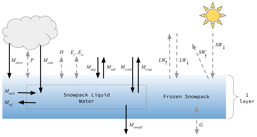
Figure 1Snow model conceptual diagram. Solid black arrows indicate mass fluxes, and dashed grey arrows indicate energy fluxes. Fluxes are described in Sect. 2.
2.1 Model overview
The SnowClim model is a fully distributed energy and mass balance snow model. It simulates the snowpack as a single layer but accounts for different surface and pack temperatures (Fig. 1). The effects of vegetation, fractional snow cover, and snow redistribution via gravitational and wind-driven processes are currently not represented.
The model has a flexible structure to facilitate uncertainty analysis and application to new conditions. This flexible structure includes tunable parameters, a customizable spatiotemporal application, and process modularity. Key parameters (Table 2) are user defined (as opposed to hard coded in the model), allowing for calibration of the model to new conditions and regions as desired. The temporal and spatial resolution and extent are also user defined, which allows users to adjust to computational constraints and the requirements of the project. Finally, key processes such as albedo and turbulent fluxes are modularized to allow evaluation of alternative process representations.
The required forcings are described in Table 1. The model can be run in MATLAB (2020b) and requires the Statistics and Machine Learning Toolbox. The code is available at https://www.hydroshare.org/resource/dc3a40e067bf416d82d87c664d2edcc7/ (last access: 14 June 2022). The model can be run in the cloud using MATLAB Online through the HydroShare Platform hosted by the Consortium of Universities for the Advancement of Hydrologic Science, Inc. (CUAHSI).
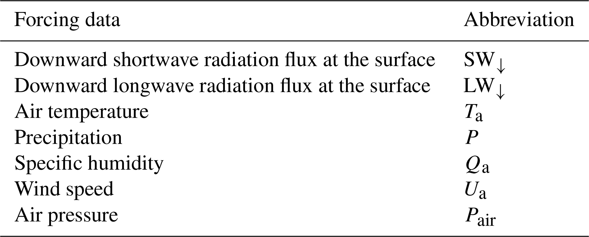
Table 2Parameters, their abbreviated names, the parameter values used in calibration, and their units. Additional parameter options, including the VIC model albedo option, were evaluated in preliminary work but were excluded from the full calibration due to consistently poor performance.
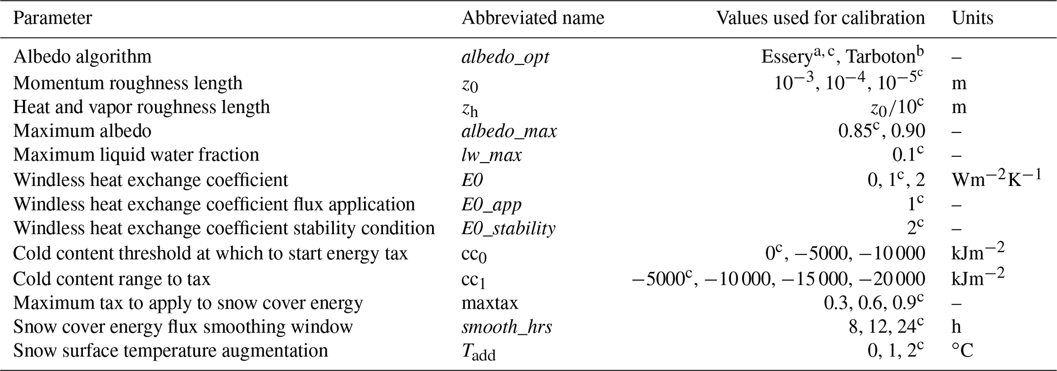
a Essery et al. (2013). b Tarboton and Luce, (1996). c Parameter values chosen for the full model run by calibration at SNOTEL sites.
2.2 Energy balance
The SnowClim model evaluates the snow cover energy balance at each time step such that
where Qnet is the net snow cover energy flux, SW↓ is the downward shortwave radiation at the surface, SW↑ is the upward shortwave radiation at the surface, LW↓ is the downward longwave radiation at the surface, LW↑ is the upward longwave radiation at the surface, H is the sensible heat flux, Ei and Ew are the latent heat fluxes of ice and water, P is the advected heat flux from precipitation, and G is the ground heat flux (Fig. 1).
2.2.1 Shortwave radiation
Upward shortwave radiation is equivalent to
where α is the spectrally integrated snow surface albedo.
Springtime snow model simulations are sensitive to the specific albedo algorithm (Etchevers et al., 2004; Günther et al., 2019). The SnowClim model provides three options for computing snow albedo (albedo_opt). In all options, albedo decays with time, and the albedo of shallow snowpacks (<100 mm depth) is diminished to account for the albedo of the ground surface, assumed to be 0.25 (Walter et al., 2005). A user-specified maximum albedo parameter (albedo_max) is used in each method.
The simplest albedo model (Essery et al., 2013; hereafter Essery) is empirical and sets albedo decay as a function of snowpack temperature. Snow albedo is augmented based on the occurrence and amount of new snow. Parameters other than the maximum albedo (minimum albedo, new snow threshold, linear and exponential albedo decline rates) are taken from Douville et al. (1995).
In the second albedo model (Hamman et al., 2018; Liang et al., 1994; hereafter VIC), snowpacks with new snow depth >10 mm and non-zero cold content receive the maximum snow albedo. Other albedo parameters are taken directly from VIC. Snow albedo decays more rapidly for melting snowpacks than cold snowpacks (cold content, cc<0).
The final albedo model (Dickinson et al., 1993; Tarboton and Luce, 1996; hereafter Tarboton) accounts for the wavelength dependence of albedo by computing separate visible and near-infrared band albedos as a function of snow surface age and solar illumination angle using a parameterization of global radiation (i.e., separate visible and near-infrared radiation are not supplied). The maximum albedo parameter is set equal to the average of the maximum visible band and infrared band albedos. This is the only albedo model of the three that includes a correction for illumination angle.
2.2.2 Longwave radiation
Upward longwave radiation is a function of snow surface temperature (Ts) in degrees Celsius, snow emissivity (ε), and the Stefan–Boltzmann constant (σ) such that
We assume ε=0.98 (Armstrong and Brun, 2008). We consider Ts to be a function of the dew point temperature (Td; Raleigh et al., 2013) such that
where Tadd is an augmentation parameter that increases Ts and improves simulations of sublimation. For further discussion of Ts, see Sect. 2.2.6.
2.2.3 Turbulent fluxes
The turbulent fluxes, H, Ei, and Ew, are estimated using a Richardson number parameterization of the exchange coefficient following Essery et al. (2013). The bulk formula are
where ρa is the air density, ca is the specific heat capacity of air, CH is the bulk exchange coefficient that accounts for near-surface atmospheric stability, Ua is the wind speed, Qs is the specific humidity of the snow surface, and Qa is the specific humidity of the air (which is a required forcing). The specific humidity of the snow surface is calculated from Ts. The exchange coefficient CH is parameterized as a function of the near-surface atmospheric stability as captured by the bulk Richardson number (RiB) such that
where g is gravitational acceleration, zu is the height of simulated wind speeds, zT is the height of simulated air temperatures, z0 is the surface roughness length for momentum, zh is the surface roughness length for heat and water vapor, and c is a constant assumed to equal 5 (Louis, 1979). Both z0 and zh are adjustable user-specified parameters (Table 2).
An optional windless exchange coefficient is available to counter large radiative losses, particularly during stable conditions (Helgason and Pomeroy, 2012; Jordan, 1991). Application of the windless exchange coefficient can be modified through three parameters: E0_value, E0_app, and E0_stability (Table 2). E0_value is the value of the windless exchange coefficient (in W m−2). E0_app controls the application of the windless heat exchange coefficient to the sensible and latent heat fluxes: an E0_app value of 1 applies the coefficient only to the sensible heat flux, whereas an E0_app value of 2 applies the coefficient to both the sensible and latent heat fluxes. E0_stability controls the type of conditions where the windless coefficient is applied: an E0_stability value of 1 applies the coefficient to all conditions, whereas an E0_stability value of 2 applies the condition only under stable atmospheric conditions.
2.2.4 Precipitation heat flux
The heat flux of liquid precipitation is
where cw is the specific heat of water, ρw is the density of water, and Prain is the rate of liquid precipitation. The heat flux of solid precipitation (S) is handled separately for diagnostic purposes and is added directly to the snowpack cold content:
where ci is the heat capacity of ice and Psnow is the rate of snowfall.
2.2.5 Ground heat flux
The ground heat flux can be important in controlling the onset of seasonal snow accumulation, particularly in warmer environments (e.g., Mazurkiewicz et al., 2008). Many process-based snow models include or couple with a soil temperature model to simulate this flux. However, under most circumstances G is thought to provide a minor contribution to the energy budget (DeWalle and Rango, 2008). In the interest of model efficiency and to avoid uncertainties associated with estimating soil temperatures and thermal conductivities, we use a constant G of 2 W m−2 (Walter et al., 2005), which is similar to other models (Etchevers et al., 2002).
2.2.6 Enhanced single-layer approach
Single-layer snow models typically provide less physically realistic snowpack simulations than multilayer models due to their simplified treatment of energy transfer within the snowpack (Blöschl and Kirnbauer, 1991; Waliser et al., 2011). Bulk single-layer conceptualizations treat the surface temperature and energy balance as synonymous with the pack temperature and energy balance, ignoring the contrast between the surface layer, which is highly sensitive to the near-surface atmosphere, and the deeper pack, which is characterized by thermal inertia, i.e., cold content. These distinctions are key to accurate modeling of snowpack heat fluxes (Blöschl and Kirnbauer, 1991) and snowpack ablation (Waliser et al., 2011).
To address these shortcomings, advanced single-layer snow models have differentiated between surface and pack temperatures, while attempting to maintain the parsimony of a single-layer model (Tarboton and Luce, 1996; You et al., 2014). To solve for snow surface temperature these approaches typically use iterative methods that can be computationally expensive (Wigmosta et al., 1994) or linearization approaches (Best et al., 2011).
The present model uses a two-step modification of the net snow cover energy flux to approximate the conduction of energy between the surface and the snowpack. This approach enables separate temperatures and energy balances for surface and pack components while retaining the computational efficiency necessary to accomplish the modeling objectives of both large spatial extent and relatively fine resolution. In this approach, the surface is conceptualized as a skin with zero depth.
First, we apply a temporal running mean to the net snow cover energy flux to approximate the attenuation with depth of the characteristic diurnal variations in energy at the surface, akin to the approach taken by You et al. (2014). The smoothed energy flux from the surface to the pack at each time step () is calculated as the average net snow cover energy flux over a period smooth_hrs, which is a tunable parameter (Table 2). This approach reduces unrealistic high-frequency modifications of the cold content and large-amplitude freeze–thaw cycles during the ablation season.
Second, we apply a progressive tax on the negative net energy flux to the snowpack to limit the excessive accumulation of cold content that results from all snow cover energy being directly translated to the pack. The net effect of the energy tax is to reduce snowpack cold content, resulting in more accurate cold content simulations relative to observations (Table A1) and similar to those from other, more complex process-based models (Jennings et al., 2018a). Other single-layer models have sought to limit cold content; however, they used approaches that required site-specific calibration (Blöschl and Kirnbauer, 1991; Braun, 1984). We apply a progressive tax such that negative energy fluxes to snowpacks with larger cold content receive larger taxes.
In Eq. (16), is the smoothed net snow cover energy flux, Qpack is the energy flux from the surface to the pack, and cc is the snowpack cold content, which uses a negative sign convention. cc0, cc1, and maxtax are tunable parameters that define the maximum (least negative) cold content to which the tax should be applied, the range of cold content over which the tax should be applied (cc0 to cc0+cc1), and the maximum possible tax, respectively (Table 2). Negative energy fluxes to snowpacks with cold contents less negative than cc0 receive zero tax, and negative energy fluxes to snowpacks with cold contents more negative than cc0+cc1 receive a tax equal to maxtax.
Qpack is added to the snowpack cold content (cc) at each time step. Pack temperature (Tpack) can be obtained from cold content as follows:
where SWE is the snow water equivalent.
2.2.7 Modification for shallow snowpacks
We developed a computationally efficient approach for controlling energy balance instabilities for shallow snowpacks. Marks et al. (1999) addressed the problem by shifting to progressively smaller time steps. In the interest of computational efficiency, we take an alternative approach. When modeled SWE is less than a threshold value, Tpack is set equal to the minimum of Ta and 0 ∘C. Cold content is then updated according to this new temperature. The threshold for applying this correction is 15 mm of SWE for every hour in the time step (e.g., for a model run at a 4 h time step, the temperature correction would be applied to snowpacks with 60 mm SWE or less). Constraining Tpack and cold content in this way is reasonable given that surface and pack temperatures are likely to be similar for shallow snowpacks and the strong correspondence between Ts and Ta (Helgason and Pomeroy, 2012).
2.3 Mass balance
The mass balance of the solid and liquid portions of the snowpack are evaluated at each time step as follows:
where Ms is the mass of the solid portion of the snowpack, Msnow is the mass of new snowfall, Mref is the mass of liquid water in the snowpack that has been refrozen, Mmelt is the mass of snow that has melted, Mdep is the mass of deposition, Msub is the mass of sublimation, Ml is the mass of the liquid in the snowpack, Mrain is the mass of rain added to the snowpack, Mrunoff is the mass of liquid water that has left the snowpack as runoff, Mcond is the mass of condensation, and Mevap is the mass of evaporation (Fig. 1).
2.3.1 Accumulation
Snowfall is calculated as an air-temperature- and relative-humidity-dependent fraction of precipitation using the bivariate logistic regression model of Jennings et al. (2018b). We use a non-binary formulation to allow for mixed-phase precipitation. New snowfall amounts less than 0.1 mm water equivalent per hour are set to 0. Rainfall is the difference between precipitation and snowfall. The temperature of new snowfall is set equal to the minimum of the dew point temperature and freezing point (0 ∘C), whereas the temperature of rainfall is set equal to the maximum of the dew point temperature and the freezing point (Marks et al., 2013; Raleigh et al., 2013).
The density of new snowfall is calculated as a function of air temperature (Anderson, 1976) using constants identified by Oleson et al. (2004). Compaction of the snowpack is modeled as a function of SWE and snowpack temperature following Anderson (1976) and using constants from Boone (2002) for the ISBA-ES snow model. Snow depth is a function of SWE and density and is updated following changes in either variable.
2.3.2 Melt
Positive net energy flux must satisfy the snowpack cold content before melt can occur. Melt is equivalent to the minimum of the current SWE and the potential melt,
where λf is the latent heat of freezing.
2.3.3 Liquid water content
Rainfall, melt, and condensation are added to, and evaporation is subtracted from, the snowpack liquid water content. Snowpack liquid water content in excess of the liquid water holding capacity of the snowpack contributes to runoff. The liquid water holding capacity of the snowpack is the product of snow depth and the maximum liquid water fraction (lw_max, Table 2). Liquid water content below this threshold but greater than the minimum liquid water content (equivalent to 1 % of snow depth; Marsh, 1991) is allowed to drain at a rate of 100 mm h−1 (based on values in DeWalle and Rango, 2008).
2.3.4 Refreezing
Excess cold content can be used to refreeze liquid water in the snowpack. The amount of water refrozen is the minimum of the total liquid water content of the snowpack and the potential refreezing,
Energy released by refreezing is added to the snowpack cold content, and the refrozen mass is added to the SWE, increasing the snowpack density (we assume no change in snow depth).
2.3.5 Sublimation and condensation
Latent heat transfer results in sublimation or evaporation from (or deposition or condensation onto) the snowpack, such that
where λs is the latent heat of sublimation and λv is the latent heat of vaporization.
The SnowClim model was evaluated and calibrated at a collection of automated snow stations across montane portions of the western US and further applied to the broader western US to create the SnowClim dataset. We describe the preparation and downscaling of the meteorological forcing data, the model calibration, and the model simulations for the western US. The model was calibrated at Snowpack Telemetry (SNOTEL) sites and model performance at these sites was used to select the parameters and temporal resolution at which to run the model over the full domain.
3.1 Spatial resolution
To balance the competing ambitions of high spatial resolution and computational feasibility over the western US domain, we used variable spatial resolutions. Regions of complex terrain were modeled at 210 m (hereafter “fine”). This high resolution enhances the model's ability to capture the effects of elevation, aspect, and slope on snowpack in complex terrain. Regions of less complex terrain were modeled at 1050 m (hereafter “coarse”). Terrain complexity was assessed for each coarse grid cell by examining the elevations and downscaled shortwave radiation values for the 25 colocated fine grid cells. If the elevation difference across the fine cells was less than 50 m and the maximum percent difference in shortwave radiation was less than 10 %, then snow simulations were completed at coarse resolution. Otherwise, simulations were completed at fine resolution. This resulted in approximately 30 % of the domain (920 605 grid cells) being modeled at coarse resolution (Fig. B1), with the remainder (64 310 454 grid cells) being modeled at fine resolution. Grid cells were defined using the 1 arcsec National Elevation Dataset Digital Elevation Model (DEM; Gesch et al., 2018) and aggregated to either 210 or 1050 m.
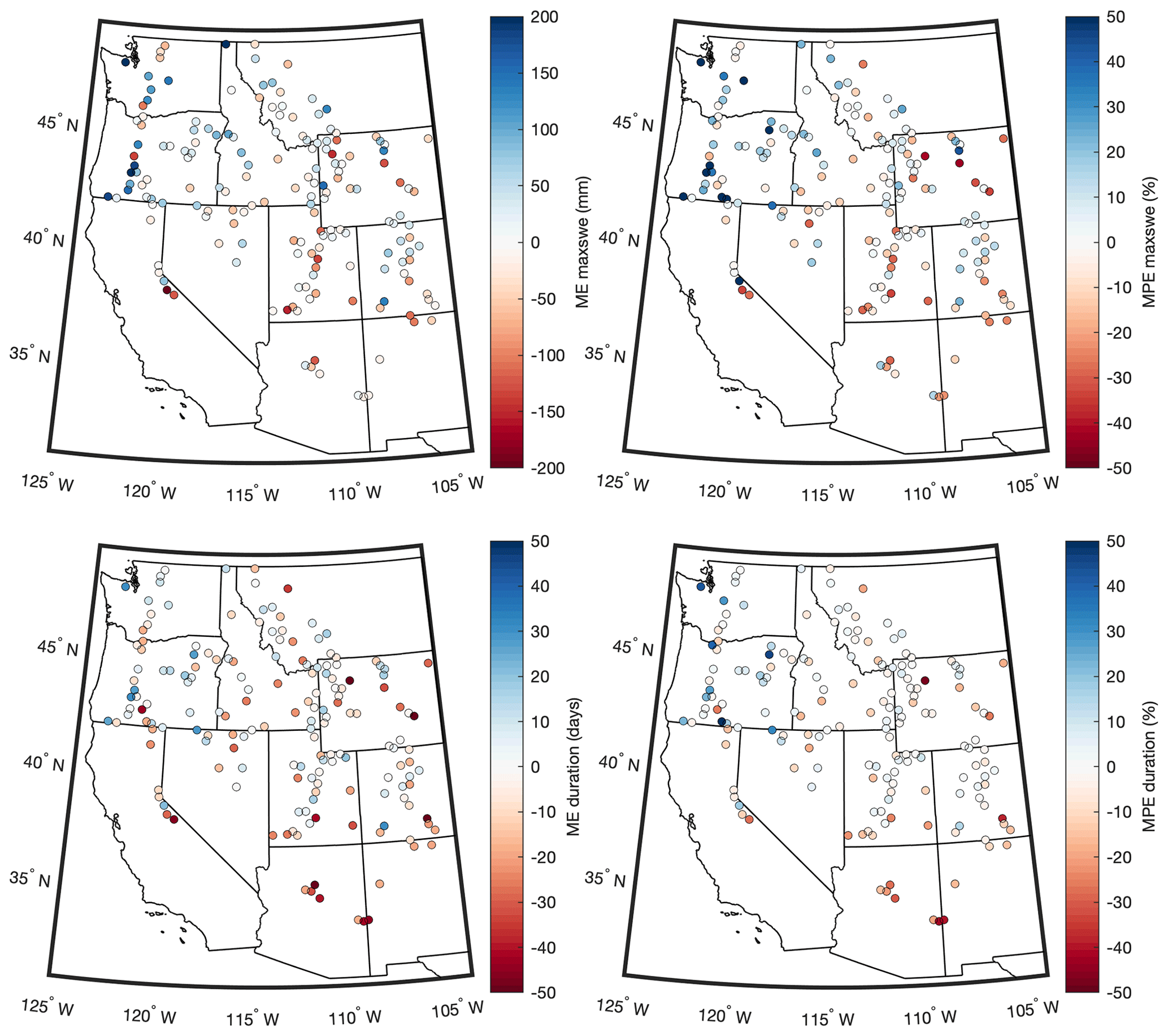
Figure 2Performance metrics for an hourly model run with the selected parameterization.
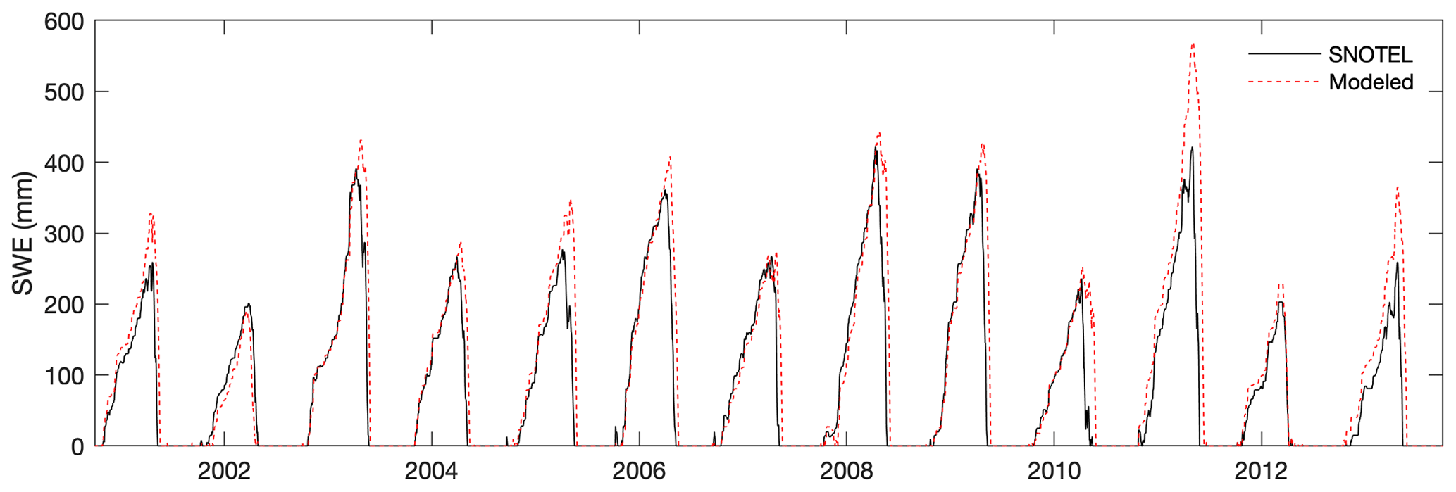
Figure 3Time series of observed and modeled SWE at the Summit Ranch, Colorado, SNOTEL site. Out of all 170 SNOTEL sites, errors at this site were closest to the all-station median errors reported in the text.
3.2 Forcing data preparation
Hourly meteorological data from the Weather Research and Forecasting model (WRF; Rasmussen and Liu, 2017) were downscaled to force the snow model (Table 3). Forcing data were developed for a historical period, future period, and pre-industrial period. The raw WRF data consisted of 4 km spatial resolution hourly simulations for 1 October 2000 to 30 September 2013 that used initial and boundary conditions from ERA-Interim (Dee et al., 2011), herein referred to as the historical period. A pseudo-global warming run was also performed by perturbing ERA-Interim by average differences from a suite of climate models participating in the Fifth Coupled Model Intercomparison Project (CMIP5; Taylor et al., 2012) between 1976–2005 and 2071–2100 under the high-warming RCP 8.5 scenario (Rasmussen and Liu, 2017). Pre-industrial forcing data were developed by perturbing the downscaled historical WRF data by monthly climatological differences in climate between pre-industrial (1850–1879) and the historical period using a pattern-scaling approach (Mitchell, 2003) based on spatially varying differences in variables from the CMIP5 models.
Table 3WRF data used to derive forcing data for the snow model.
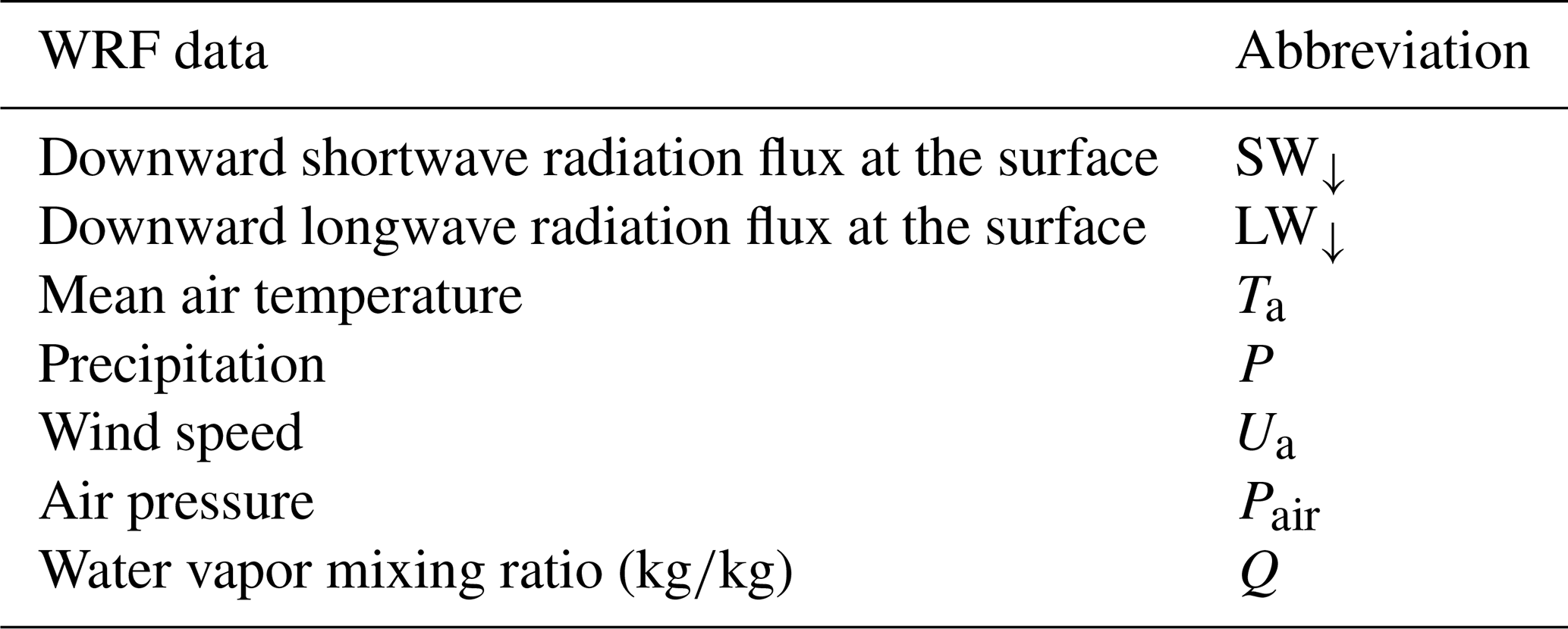
Spatial downscaling for all variables except shortwave radiation was accomplished using moving window lapse rates (i.e., the change in the variable with elevation). Lapse rate downscaling has been shown to perform well relative to other statistical downscaling approaches in mountainous terrain (Praskievicz, 2018; Wang et al., 2012). We estimated monthly lapse rates for each grid cell and each variable, except for temperature, for which we estimated hourly lapse rates for each grid cell. Windows of 7×7 WRF grid cells (or 28×28 km) were used to balance the competing objectives of sufficient data points and the ability to capture local phenomena (Lute and Abatzoglou, 2021). Lapse rate corrections were applied hourly using the elevation difference between the WRF grid cell and the target DEM grid cell. For air pressure, lapse rates were calculated from and applied to temporally averaged WRF data. Grid cells not classified as land by WRF were excluded from lapse rate calculations.
For precipitation, a modified version of the methods above was used. Prior to calculating lapse rates, WRF precipitation was bias corrected to monthly 4 km precipitation from PRISM (PRISM Climate Group, 2015) by calculating monthly correction ratios, i.e., the ratio of total monthly PRISM precipitation to total monthly WRF precipitation. Correction ratios were set to 1 (no correction) when monthly WRF precipitation was 0 or when the ratio was infinite. Monthly precipitation lapse rates were divided by the number of hours with precipitation each month in the underlying WRF data, and hours with zero precipitation were maintained in the downscaled data to avoid precipitation every hour due to non-zero monthly lapse rates.
Shortwave radiation was downscaled to the target DEM using the insol package in R (Corripio, 2015) following the approach of Lute and Abatzoglou (2021), which preserves the atmospheric effects (e.g., cloud cover) captured by WRF and also accounts for slope, aspect, self-shading, and shading by adjacent terrain. Parameters required by the algorithm, including visibility, RH, and temperature, were assumed to be constant. Terrain corrections were calculated for the midpoint of each hour of the middle day of each month, aggregated to the desired temporal resolution using a weighting scheme based on the amount of solar radiation each hour, and then interpolated to the full time period.
For model calibration at SNOTEL sites (see Sect. 3.3.2), the above downscaling procedures were applied, but values were adjusted based on the elevation difference between the SNOTEL site and the colocated WRF grid cell based on calculated lapse rates. Downscaled WRF precipitation was bias corrected to SNOTEL sites by applying a monthly correction factor consisting of the ratio of the total SNOTEL precipitation to the total WRF precipitation similar to Havens et al. (2019). We note that such bias correction approaches may not address issues of precipitation undercatch at SNOTEL sites.
Additional variables needed to force the snow model, including specific humidity, relative humidity, and dew point temperature, were derived from the downscaled WRF water vapor mixing ratio, air temperature, and air pressure data using standard methods. Dew point temperatures exceeding the air temperature were set equal to the air temperature.
Table 4Spatial correlations (R2) between observations at SNOTEL sites and SnowClim simulations for various snow metrics over the model calibration period 1 October 2000–30 September 2013.
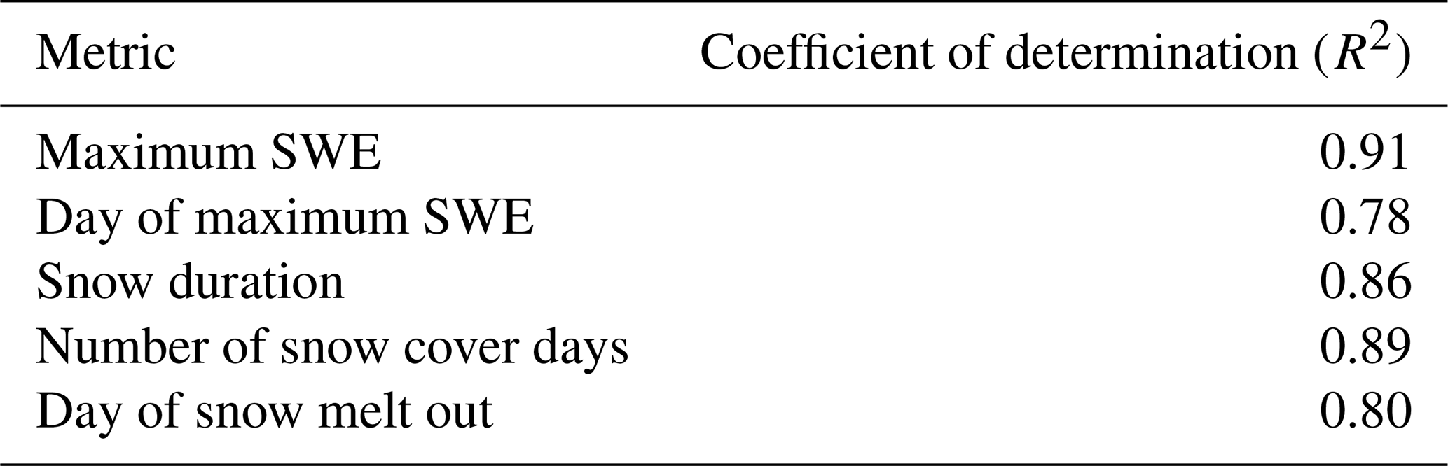
Table 5Summary climate and snow variables included in the SnowClim dataset. Summary variables are available for pre-industrial, historical, and future time periods.
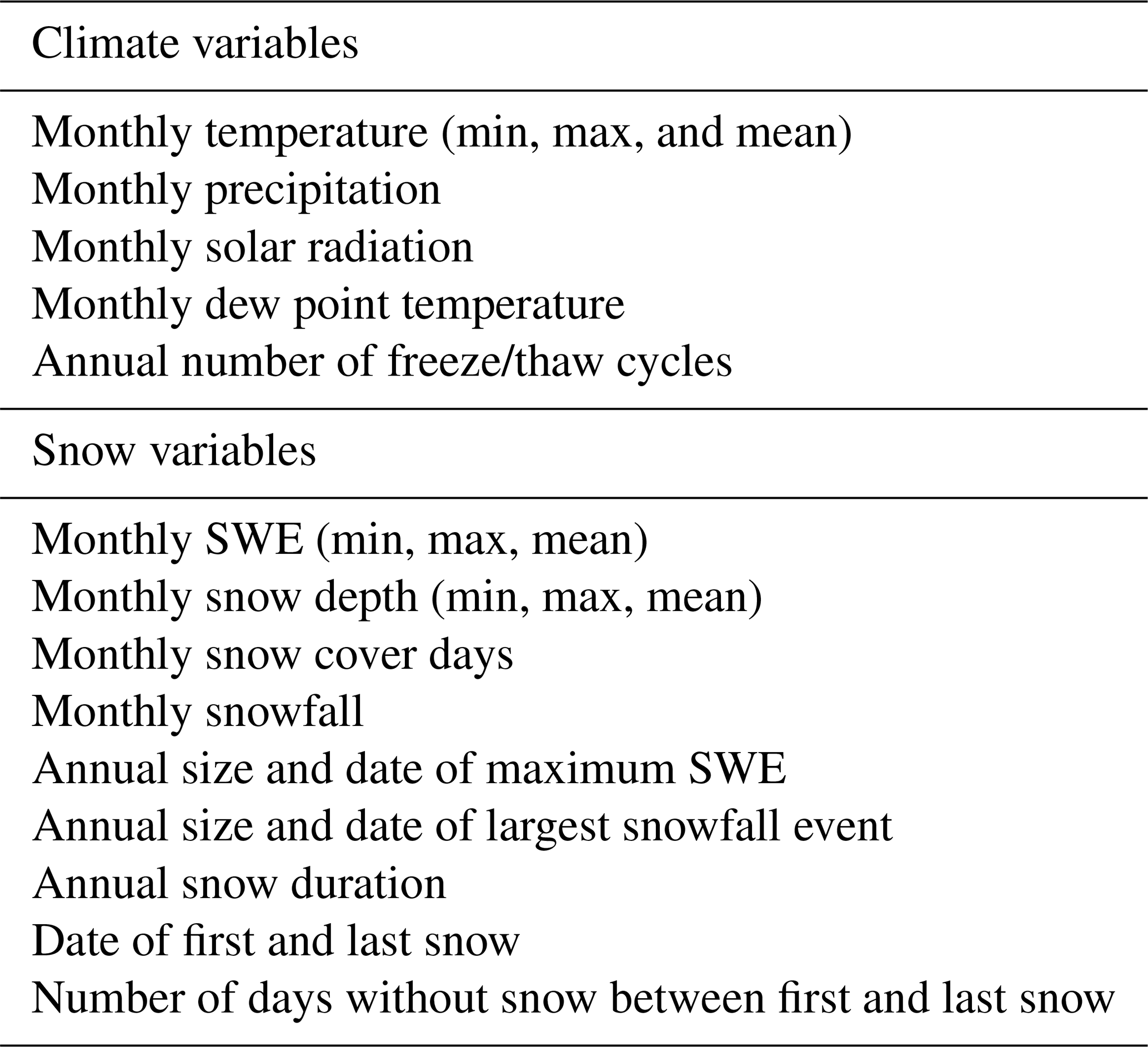
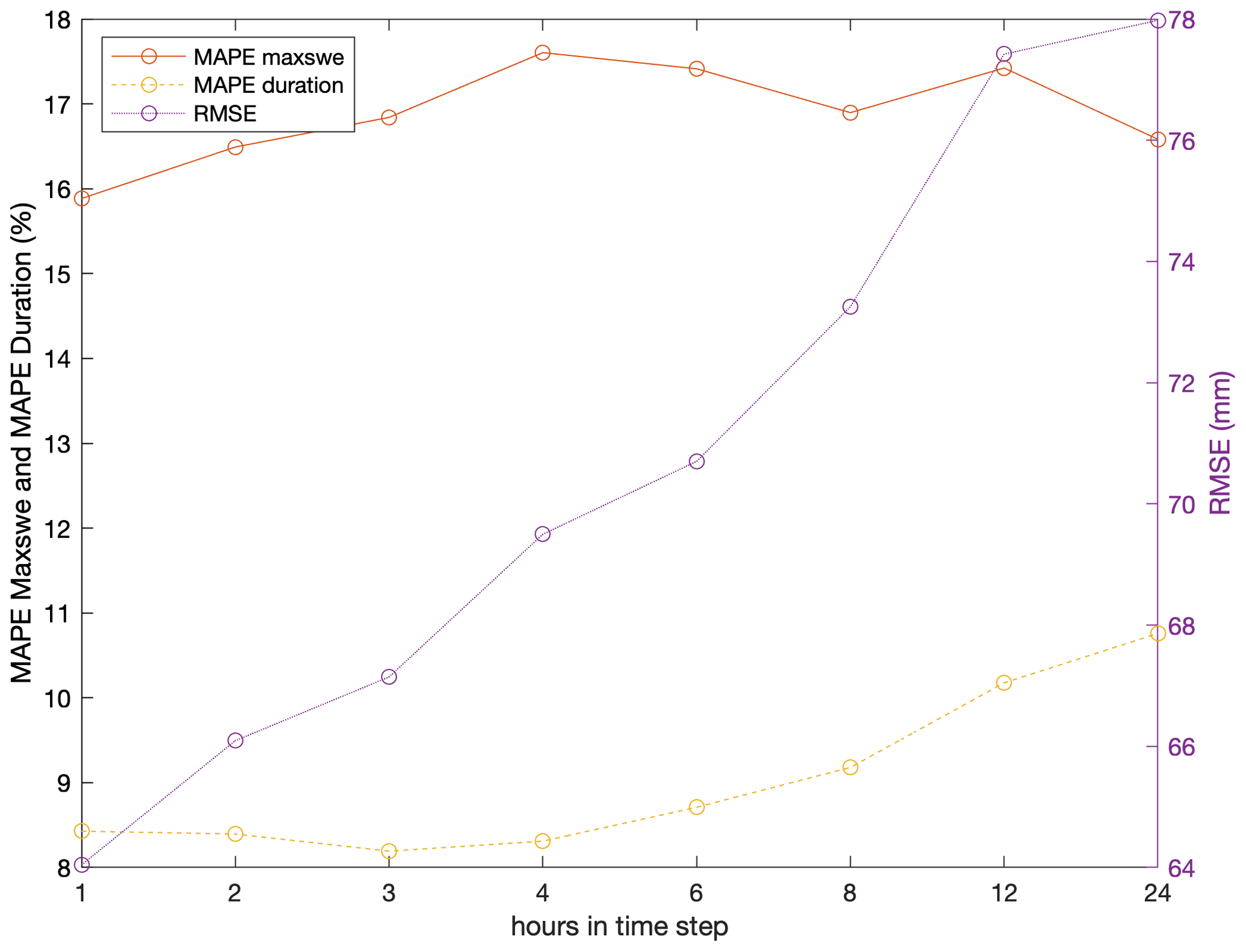
Figure 4Snow model performance for different time steps using the parameter set selected in calibration of the hourly model. Points represent median values across 170 SNOTEL sites.
3.3 Model calibration
3.3.1 Calibration methods
The model was calibrated at SNOTEL sites across the mountains of the western US to select a single best parameter set across all sites. While the SNOTEL network may not be perfectly representative of the broader domain (Molotch and Bales, 2005), it represents the best available ground observation dataset for calibration purposes due to the number of sites, range of hydroclimate conditions monitored, length of record, and relatively consistent observational methods and equipment across sites. A total of 170 SNOTEL sites were selected meeting the following requirements:
-
an elevation difference of less than 75 m relative to the colocated WRF grid cell,
-
a dataset missing no more than 1 % of daily precipitation and SWE observations between October and May in every water year between 1 October 2000 and 30 September 2013,
-
a site located more than 25 km from any other SNOTEL site.
Missing SWE values were infilled using linear interpolation across time. Missing precipitation values were infilled using an inverse distance weighted average of the values at the three closest sites.
Calibration consisted of running the model across all SNOTEL sites for each possible combination of parameters listed in Table 2. Model performance was assessed using the mean absolute percent error (MAPE) of annual maximum SWE (maxswe), the MAPE of annual snow duration, and the root-mean-squared error (RMSE) of daily SWE at each site. Snow duration was defined as the duration (in days) of the longest period of consecutive days with SWE >0. RMSE was computed for days when observed SWE exceeded 10 mm. Additionally, we used the mean error (ME) and mean percent error (MPE) of maxswe and duration to visualize calibration errors. The optimal parameter set was selected using Pareto preference ordering (Khu and Madsen, 2005) based on the median of each statistic across stations.
The model was subsequently evaluated for different run time steps (1, 2, 3, 4, 6, 8, 12, and 24 h). Separate model calibration for each time step selected similar parameter sets to the hourly run, and thus the hourly parameter set was used for all time steps. Model performance was again assessed as described above.
3.3.2 Calibration results
Snow model calibration via Pareto optimization selected a single best parameter set (Table 2). The station median MAPE of maxswe, MAPE of snow duration, and daily RMSE for this parameter set were 15.9 %, 8.43 %, and 64.0 mm, respectively. The spatial distribution of ME and MPE in maxswe and duration lacked strong coherent spatial patterns (Fig. 2), and spatial correlations (R2) for a variety of snow metrics exceeded 0.75 (Table 4), suggesting that the model captured major climate-related effects and sources of large-scale spatial snow variability. The largest negative biases were found at drier sites with relatively shallow or intermittent snowpacks (Fig. B2). The largest positive biases were found at sites with mean winter temperatures at or above freezing, where snow accumulation is very sensitive to the partitioning of precipitation into rain vs. snow (Fig. B2). A time series of observed and modeled SWE at one site with error values close to the station median values illustrates the model performance on a daily scale (Fig. 3). The model also captured key components of interannual snowpack variability over the short historical period; the station median correlation coefficients for maxswe and for snow duration were 0.93 and 0.70, respectively. The station correlations did not demonstrate any clear geographic or climatic patterns. This lends confidence to the model's ability to accurately simulate snow dynamics across a range of climates. The parameter sensitivity of the model is shown in Fig. B3.
Model performance deteriorated as temporal resolution coarsened from 1 to 12 h but improved slightly for the 24 h time step (Fig. 4). Model performance was somewhat sensitive to the hours used for aggregation; other aggregation windows showed continuous performance deterioration with coarsening temporal resolution (not shown). The sensitivity of model performance to the aggregation window is likely related to how diurnal energy fluxes, particularly shortwave radiation, are aggregated. A time step of 4 h was selected for the full western US model run to balance the objectives of computational efficiency and model performance. The station median MAPE of maxswe, MAPE of snow duration, and RMSE for the 4 h time step were 17.6 %, 8.31 %, and 69.5 mm, respectively. We note that simulations without the modification for shallow snowpacks (Sect. 2.2.7) degraded more consistently and significantly with coarsening temporal resolution (Fig. B4).
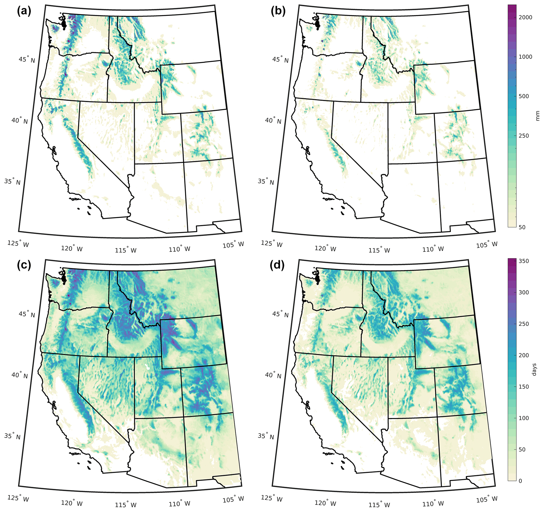
Figure 5(a) Historical and (b) future maxswe (mm), (c) historical and (d) future snow duration (days). Historical values are averages over the period 2000–2013. Future values represent averages during the period 2071–2100 under RCP 8.5. In (a) and (b), white land areas denote areas that had less than 50 mm maxswe. In (c) and (d), white land areas denote areas where snow duration was 0. Note the nonlinear color scale in panels (a) and (b).

Figure 6(a) Absolute and (b) percent change in maxswe between historical and future periods. (c) Absolute and (d) percent change in snow duration between historical and future periods. In (d), small boxes in Utah and Colorado indicate the regions highlighted in Figs. 7 and 8, respectively.
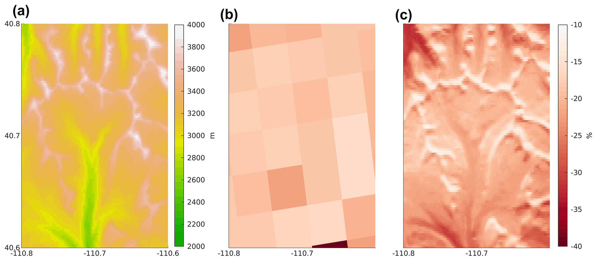
Figure 7Example of simulations of changing maxswe for a portion of the Uinta Mountains, Utah (location is marked in Fig. 6). The elevation (m) of the domain is shown in (a). The percent change (%) in maxswe between historical and late 21st century periods as simulated by a 4 km WRF product (Rasmussen and Liu, 2017) is shown in (b), and the same metric but from the SnowClim dataset is shown in (c).
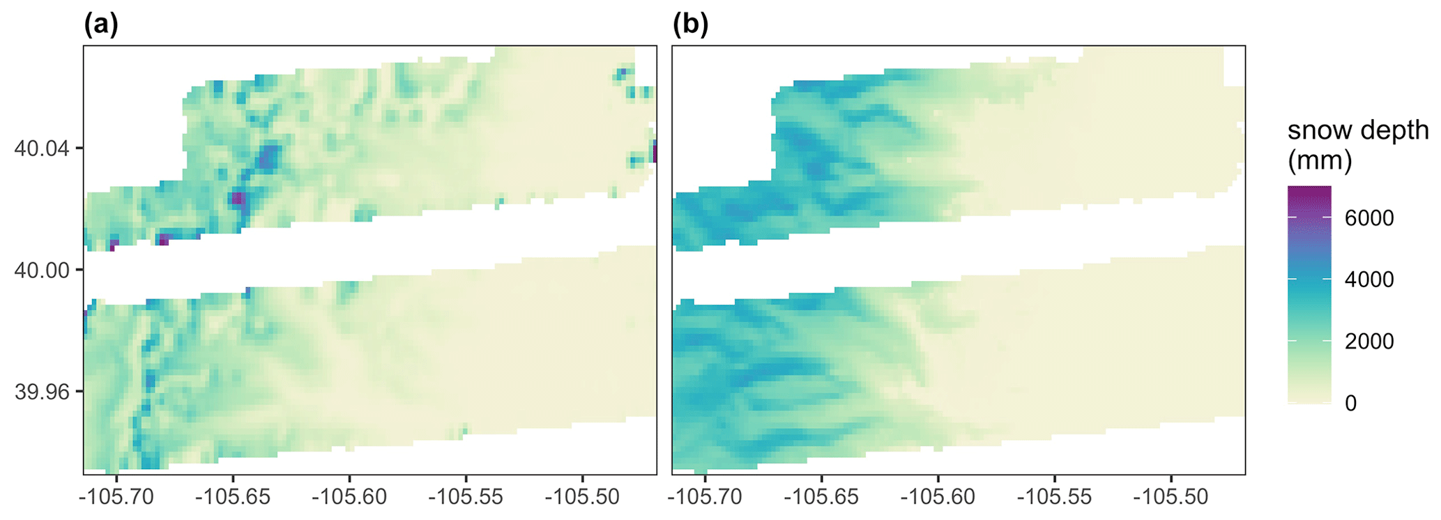
Figure 8Snow depth on 20 May 2010 in the Boulder Creek Watershed area indicated in Fig. 6 from (a) lidar (described in Harpold et al., 2014) and (b) SnowClim.
3.4 Model results for the western United States
The SnowClim model was applied to the western US (contiguous US west of 104∘ W) using the parameters identified above, a temporal resolution of 4 h, and a variable spatial resolution as described previously (210–1050 m horizontal resolution). The model was run in parallel on a high-performance standalone server (Dell Poweredge R730) with 34 cores and 128 GB RAM. The compute time for downscaling the climate forcings and executing the snow model was 10 and 2.5 d, respectively, for the historical period. For reference, the model took less than 0.03 s per site year when run using a single core across the 170 SNOTEL sites.
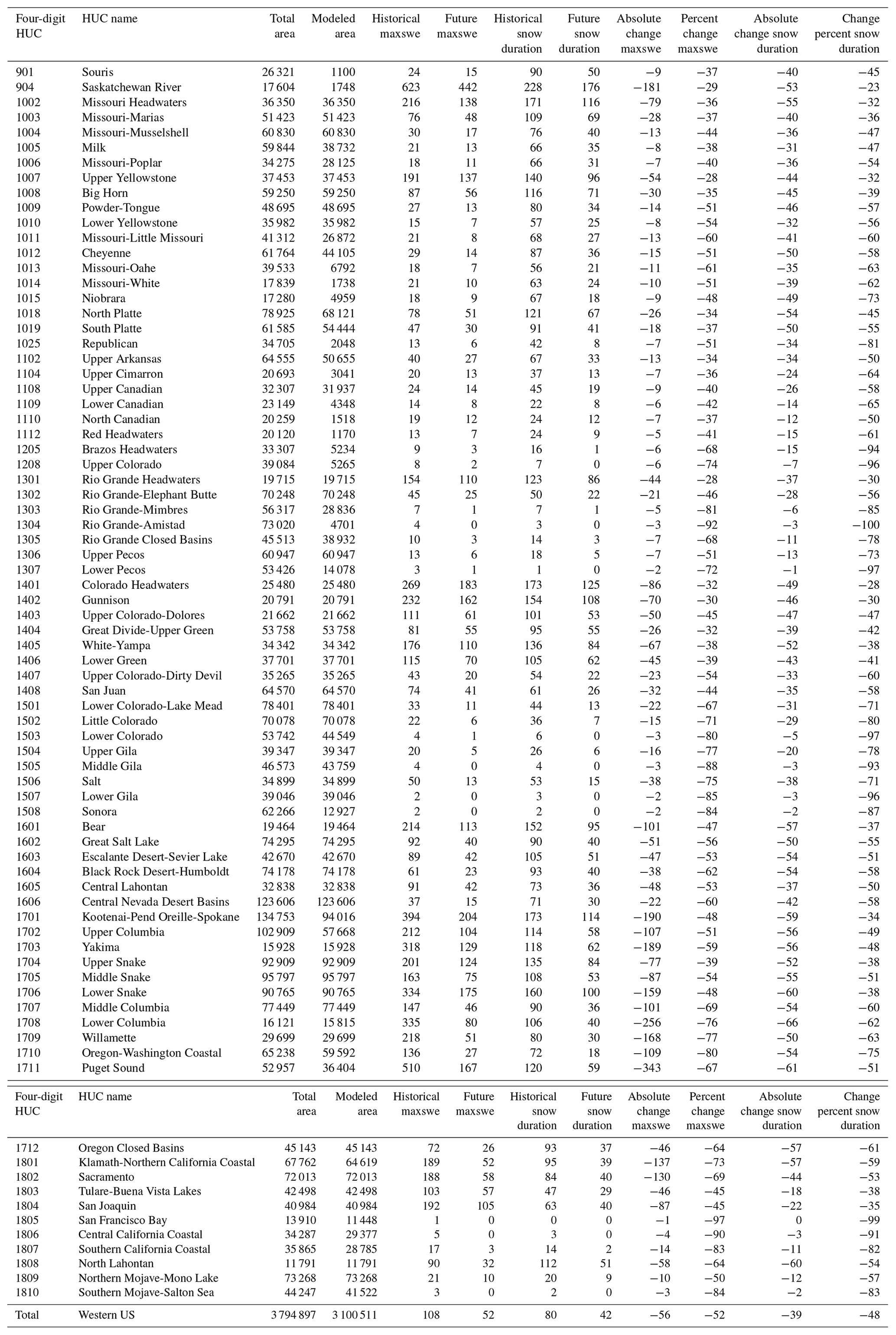
Large-scale spatial patterns of climatologies and changes in maxswe and snow duration (Figs. 5 and 6) were broadly similar to those from existing products developed from a wide range of modeling approaches (Luce et al., 2014; Lute et al., 2015; Ikeda et al., 2021). Historical maxswe was 112 mm, spatially averaged across the full western US domain, and locations with historical maxswe <50 mm were found in the warmer southern and southwestern regions and in the northeastern portion of the domain where winters are relatively dry (Fig. 5a). Under the future scenario, spatially averaged maxswe declined to 54 mm, and the areas with maxswe <50 mm expanded to encompass many lower-elevation areas (Fig. 5b). Historical snow duration averaged 83 d, spatially averaged across the full western US domain (Fig. 5c), but declined to 43 d in the future scenario (Fig. 5d). There were only a handful of locations with increases in maxswe or duration in the future period compared with the historical period, and these increases were small (Fig. 6). The largest relative declines in maxswe and duration were found at low elevations. On average, maxswe decreased by 49 % across locations with at least 50 mm maxswe historically, and snow duration decreased by 61 % across locations with historical snow duration greater than zero. Summaries of historical and future maxswe and duration by four-digit hydrologic unit code (HUC) are provided in Table B1.
Compared to existing large extent, multitemporal, process-based snow datasets such as that from the 4 km WRF runs (Rasmussen and Liu, 2017), SnowClim provided a much more nuanced picture of changing snow, particularly in areas of complex terrain. For example, Fig. 7 shows relative changes in maxswe for the Uinta Mountains in northeastern Utah as simulated directly by the 4 km WRF product and by SnowClim. SnowClim captured effects of elevation and aspect, including greater percent reductions in maxswe at lower elevations and on south-facing aspects, similar to Barsugli et al. (2020). Nuanced results such as these are only possible with high-resolution snow modeling that explicitly simulates spatiotemporal variations in the dominant snow cover energy fluxes.
Comparison of SnowClim snow depth with a snapshot of finer-resolution lidar-based observations further highlights some of the strengths and limitations of SnowClim. For example, in the Boulder Creek Watershed, Colorado, SnowClim captured the broad-scale spatial patterns of snow depth that are present in lidar-derived depth observations (described in Harpold et al., 2014) aggregated from the original 1 m resolution to the resolution of SnowClim on 20 May 2010 (Fig. 8). However, SnowClim snow depth was less spatially variable, particularly in the higher-elevation western portion of the domain. Evaluations such as this are particularly challenging as they simultaneously evaluate the spatial and temporal fidelity of the forcing data, the snow model, and in particular the snow density algorithm. The muted spatial variability in SnowClim can be attributed to a combination of factors, chief of which may be the lack of wind–snow interaction in the current SnowClim model formulation. Snow redistribution by wind and blowing snow sublimation have a significant effect on snowpack heterogeneity in this region (Knowles et al., 2012; Sexstone et al., 2018; Winstral et al., 2002); one study showed that a model incorporating wind redistribution captured 8 %–23 % more of the spatial variability in snow depth than a model without these processes (Winstral et al., 2002). In order to better simulate snowpack in windy environments such as the alpine area shown here, incorporation of blowing snow transport and sublimation into future SnowClim model formulations should be considered.
Through the development of a new computationally efficient snow model, SnowClim, and novel forcing data, we have overcome the two major hurdles to achieving snow data that meets the criteria outlined in Sect. 1. SnowClim's distinctive balance of mostly process-based and some empirical components allows it to capture contrasts in radiative loading in complex terrain, timing and rate of ablation, and responses to future climate, while maintaining computational efficiency. The SnowClim dataset is spatially continuous across the western US at sub-kilometer resolution in complex terrain, enabling both high-resolution and large-extent analyses. In particular, the SnowClim model and dataset highlight the effects of elevation and aspect on snowpack in a changing climate. The inclusion of multiple snow variables and compatible climate variables across multiple time periods will empower analyses of hydroclimatic responses to changing climate and complement existing coarser-resolution products.
The SnowClim model excludes some processes that might be included in more complex, computationally expensive large-scale models (e.g., VIC, WRF) such as vegetation-related processes, blowing snow transport and sublimation, and gravitational redistribution. In some contexts, these processes may be necessary for accurate modeling of the snowpack (Freudiger et al., 2017; Musselman et al., 2008; Pomeroy et al., 1993). The western US SnowClim dataset was calibrated at SNOTEL sites, which are often in forest clearings, and it is therefore expected to be relatively accurate in similar environments. However, user judgment should be applied when using the model or dataset in vegetated areas. Given the complexity of vegetation–snow processes, incorporation of vegetation effects may add significant computational expense and is hindered by the need for vegetation-related data and parameters that are expected to change between the time periods considered here. Future vegetation change is subject to large uncertainty stemming from disturbance regimes and species composition pathways. However, incorporation of an optional vegetation routine to be used when data and computational resources are available is a logical next step. Approaches for incorporating blowing snow transport either require (i) high-resolution wind fields input to semi-empirical or 3D turbulent-diffusion models (summarized in Mott et al., 2018), requiring more sophisticated downscaling of wind fields than what was done here and substantially increasing computational cost, or (ii) require calibration of terrain parameters (e.g., Winstral et al., 2013), which would be possible but both challenging and computationally intensive for a large-scale model such as SnowClim. Simple algorithms do exist for modeling gravitational redistribution of snow (Bernhardt and Schulz, 2010); however, incorporation of either blowing snow transport or avalanching would necessitate restructuring of the model as a semi-distributed or fully distributed model with spatial interaction, which by itself would likely reduce the computational efficiency of the model. The model also includes simplified representations of the ground heat flux and snow surface temperature, which may be better captured by more process-based approaches. In particular, a more nuanced treatment of the ground heat flux may be desired in warmer snow climates (Mazurkiewicz et al., 2008).
Contrasts between modeled and observed snow metrics stem from several factors, including (but not limited to) uncertainties in climate forcings, SNOTEL-site-specific factors that the model neglects such as fine-scale topographic and vegetation patterns, and errors in model specification such as process representation and calibration. Despite these factors, errors at SNOTEL sites from the hourly SnowClim model run were relatively small and compared well with errors reported for other gridded snow products. Ikeda et al. (2021) evaluated the snow simulations from the same 4 km WRF model runs that we used to source our raw climate forcings (Rasmussen and Liu, 2017). Relative to SNOTEL sites, they found a −26.2 % bias in maxswe. In contrast, the SnowClim model achieves a maxswe bias of only 0.15 %. Wrzesien et al. (2018) compared maxswe at SNOTEL sites to maxswe from 9 km WRF simulations. Across sites, they found a correlation coefficient of 0.55 and a bias of −89 mm. SnowClim achieves a correlation coefficient of 0.94 and bias of −11 mm. In the Californian Sierra Nevada, Guan et al. (2013) blended modeled, remotely sensed, and observed data to capture SWE at six sites. Their method achieved a SWE RMSE of 205 mm compared to snow surveys. The SnowClim mean RMSE of daily SWE was 77 mm across all sites and 166 mm at Sierra Nevada sites. While errors at SNOTEL sites were generally low, the model did tend to overestimate maxswe and duration at some warm and wet sites and underestimate these metrics at dry sites (Fig. B2). Further evaluation of the parameters used here in more marginal snow environments would lend additional confidence to the application of SnowClim data in these areas. While the model's excellent performance relative to SNOTEL observations is in part due to the fact that the model was calibrated to SNOTEL data, the model could be calibrated to other observations for application in other contexts.
The flexible, modularized structure of the SnowClim model lends itself to calibration, parameter sensitivity assessment, and experimentation. In the western US, model performance was particularly sensitive to the choice of albedo algorithm and snow surface temperature parameterization, in line with previous findings (Etchevers et al., 2004; Günther et al., 2019; Slater et al., 2001; Fig. B3). Given the importance of impurities (e.g., tree litter, dust, and black carbon) on snow albedo and consequently snow melt (Waliser et al., 2011), a future step will be to add albedo algorithms that account for these effects. The modular structure of SnowClim would make this relatively straightforward.
Given the multifaceted importance of snow and ongoing snowpack changes due to climate change, there is a need for models that can accurately and efficiently simulate snow to generate spatially extensive, high-resolution datasets to meet the diverse requirements of different applications. We anticipate that the SnowClim model and data will be powerful tools for researchers and managers across a range of disciplines, including ecology and wildlife biology, recreation, transportation, hazard planning, and glacier and hydrologic modeling. The SnowClim model and data will be particularly useful for applications requiring high spatial resolution data, such as species distribution and refugia modeling, and will complement the existing array of snow models and datasets by providing a novel balance of process-based elements and computational efficiency.
We compared observed cold content and cold content simulated using SnowClim (both with and without the tax approach) at two sites in the Niwot Ridge Long-Term Ecological Research site (LTER), Colorado: an alpine site (Saddle) and a subalpine site (C1). The cold content observations are presented in Jennings et al. (2018).
For the comparison, we ran SnowClim at each of the sites using hourly observed climate forcings from the sites (Jennings et al., 2021) for water years 2001–2013. The model was first run with the cold content tax described in Sect. 2.2.6 (i.e., as reported in this paper). Following this, an additional run was performed in which the tax approach was turned off. The goal of this experiment was to evaluate how well the model simulates cold content relative to observations and to determine whether the tax approach improved cold content simulations compared to the same model without the tax approach. The same parameters from the western US run were used for modeling these sites, and the model was not recalibrated. Simulated cold content was smoothed using a 2-week moving mean to provide a more robust comparison to observations, which were collected at weekly to monthly intervals. Peak (minimum) cold content values were averaged across years to get a peak cold content value for each site and model run, and these were compared with the peak cold content values from observations reported in Jennings et al. (2018), Table 1.
Despite scale discrepancies between point observations and 210 m grid cells, SnowClim peak cold content compares well with observations when the tax approach is used. In contrast, when the tax approach is not used and all negative energy fluxes are directly added to the pack cold content, cold content becomes an order of magnitude greater than the observations.
Table A1Comparison of peak seasonal cold content values from observations, SnowClim simulations including the tax approach described in Sect. 2.2.6, and SnowClim simulations without the tax approach at two sites from the Niwot Ridge Long-Term Ecological Research site in Colorado.
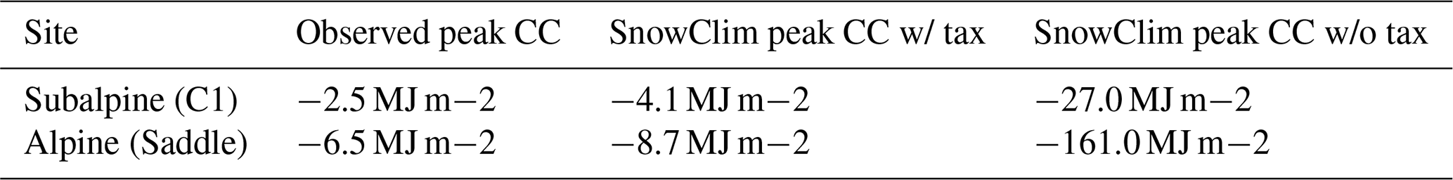
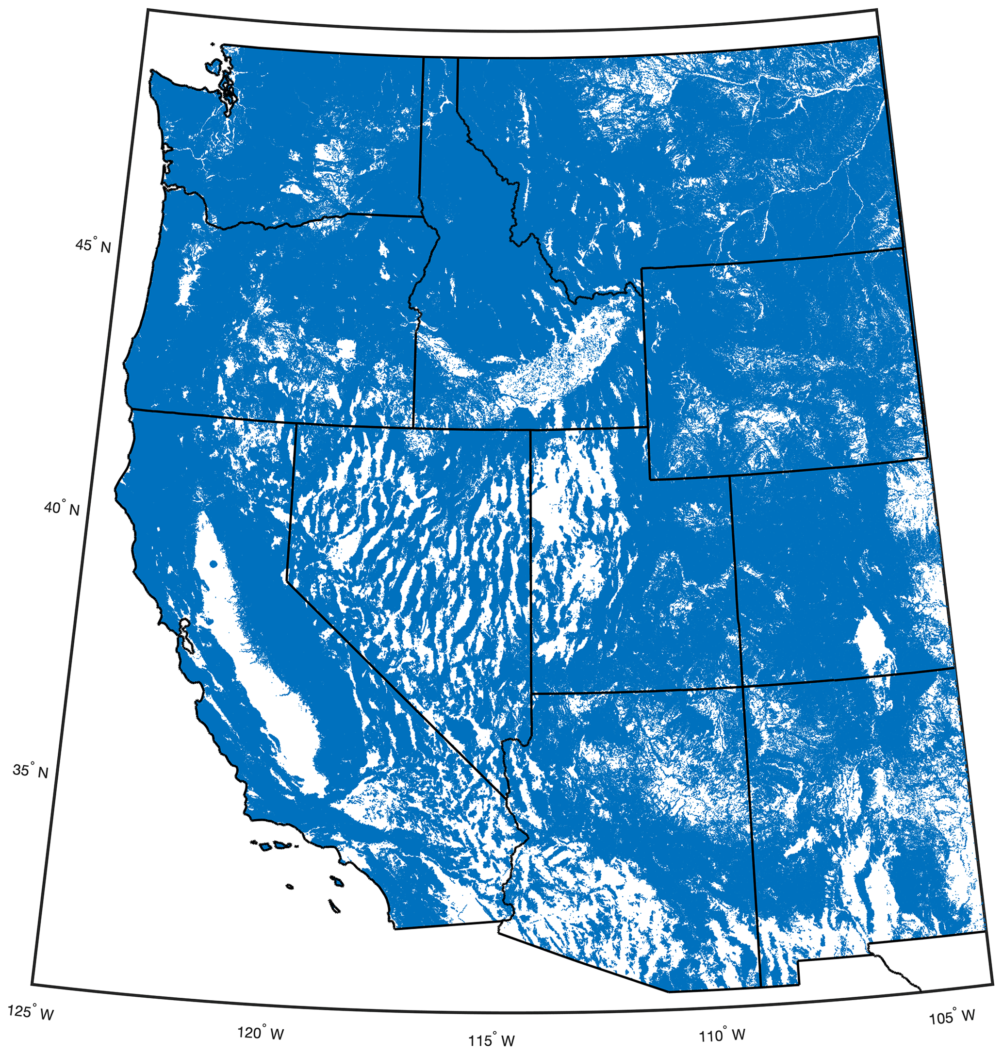
Figure B1Map of the 3.1 million square kilometer modeling domain with locations modeled at 210 m spatial resolution shown in blue.
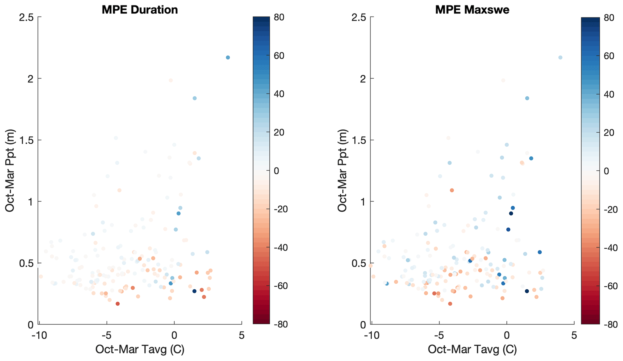
Figure B2Performance of the best hourly model at SNOTEL sites in temperature–precipitation space. Each point represents a SNOTEL site.
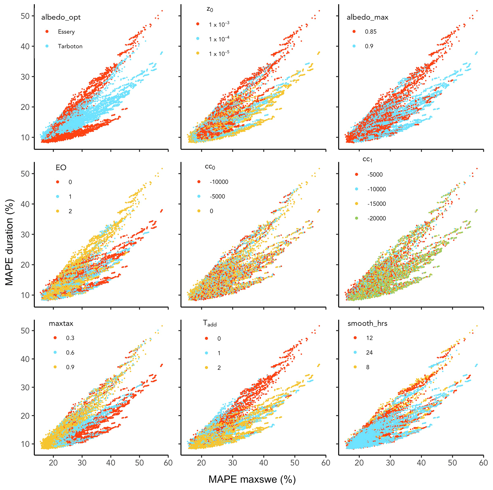
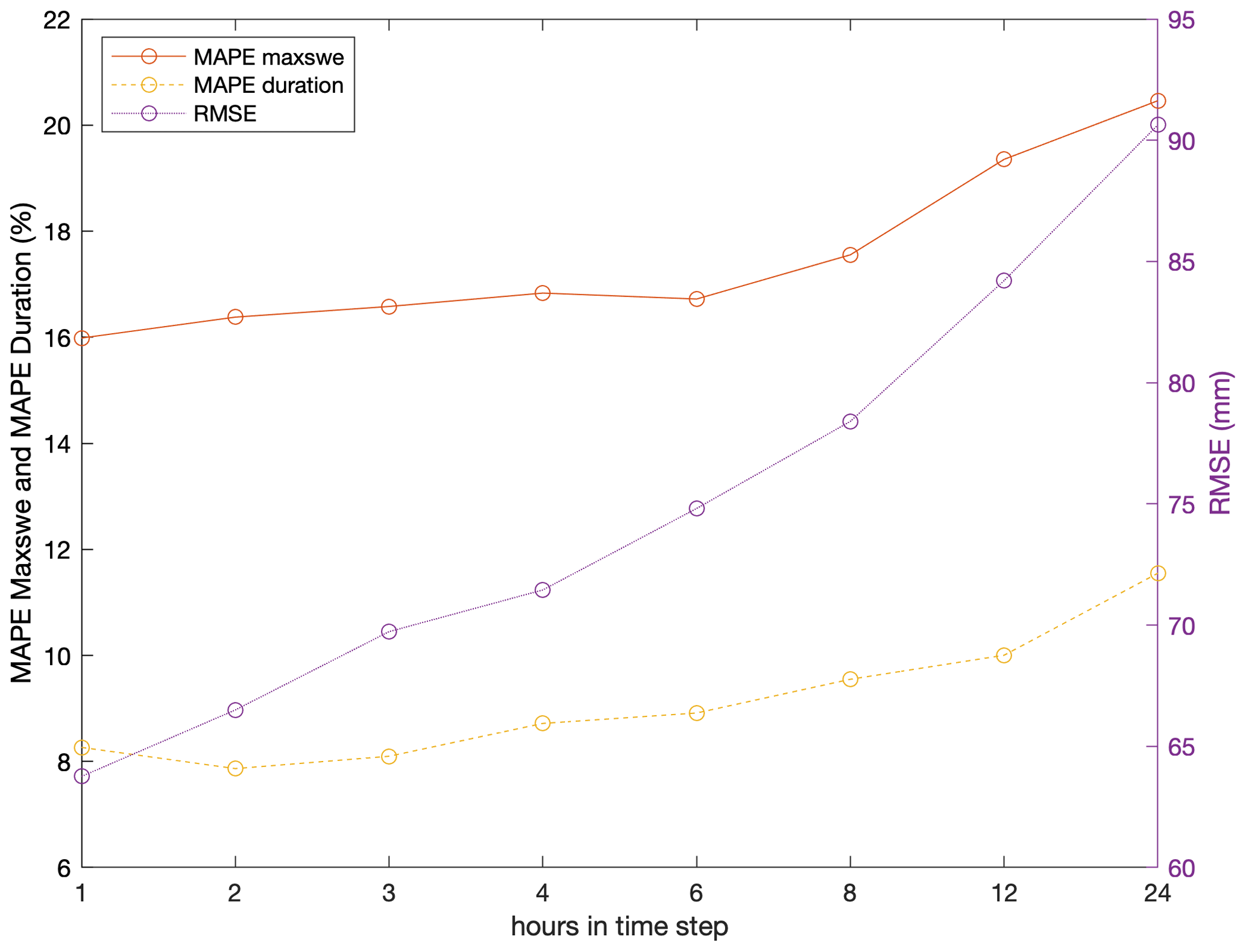
Figure B4Performance of the snow model without shallow snow correction for different time steps using the parameter set selected in calibration of the hourly model with shallow snow correction. Points represent median values across 170 SNOTEL sites.
Table B1Summary of snow metrics by four-digit HUC. Total and modeled areas are in square kilometers, maxswe has units of millimeters, and snow duration has units of days. Values are averaged over all modeled grid cells within each HUC. Total snow metric values (in the last row) are averaged across all grid cells across the western US modeling domain, and total changes are computed from these total snow metric values.
The code for the SnowClim model is available from https://doi.org/10.4211/hs.acc4f39ad6924a78811750043d59e5d0 (Lute et al., 2021) under the Creative Commons Attribution CC BY. The model can be run using MATLAB Online through HydroShare. The code is also available on Dryad at https://datadryad.org/stash/share/wywmnpELgnP0b3joYVccmZJ0TKvgNsIh7PjQuz3FjXM (last access: 14 June 2022).
Climate forcing data and modeled snow variables were aggregated to monthly and annual climatologies for each time period to create the SnowClim dataset (Table 5). These data are available from https://doi.org/10.4211/hs.acc4f39ad6924a78811750043d59e5d0 in both netCDF and geoTIFF formats (Lute et al., 2021). The data are additionally available in netCDF format on Dryad at https://datadryad.org/stash/share/wywmnpELgnP0b3joYVccmZJ0TKvgNsIh7PjQuz3FjXM (last access: 14 June 2022).
ACL developed the model code with input from JA and TL. ACL developed the downscaling code with input from JA. ACL performed the downscaling, calibration, and snow model simulations. ACL prepared the manuscript with contributions from JA and TL.
The contact author has declared that neither they nor their co-authors have any competing interests.
Publisher's note: Copernicus Publications remains neutral with regard to jurisdictional claims in published maps and institutional affiliations.
We thank two anonymous reviewers for their thorough and constructive feedback on an earlier version of this paper.
This research was conducted on the homelands of the Nimiipuu (Nez Perce) at the University of Idaho in Moscow, Idaho. The University of Idaho is a land grant university whose endowment was partially funded by more than 350 km2 of land acquired through the Morrill Act. The United States government used treaties and seizures to obtain land from the Shoshone-Bannocks, Nimiipuu, and Schitsu'umsh (Couer d'Alene) tribes. The income generated from this land, benefitting the university, is 372 times the amount paid to the tribes (Lee, 2020). Additionally, data used in this research was collected on land significant to many Indigenous communities across the western United States. The authors recognize, pay respect, and extend gratitude to the Indigenous communities that live upon, hold sacred, and care for the lands reflected in this research.
This research has been supported by the National Science Foundation (grant no. 1249400) and CUAHSI with support from the National Science Foundation (grant no. EAR-1849458).
This paper was edited by Andrew Wickert and reviewed by two anonymous referees.
Abatzoglou, J. T. and Brown, T. J.: A comparison of statistical downscaling methods suited for wildfire applications, Int. J. Climatol., 32, 772–780, https://doi.org/10.1002/joc.2312, 2012.
Anderson, E. A.: A point energy and mass balance model of a snow cover, NOAA Technical Report NWS 19, National Weather Service, 150 p., https://repository.library.noaa.gov/view/noaa/6392 (last access: 1 June 2021), 1976.
Anderson, E. A.: Snow Accumulation and Ablation Model – SNOW-17, US National Weather Service, Silver Spring, MD, 61 p., https://www.weather.gov/media/owp/oh/hrl/docs/22snow17.pdf (last access: 1 June 2021), 2006.
Armstrong, R. L. and Brun, E.: Snow and Climate: Physical Processes, Surface Energy Exchange and Modeling, Cambridge University Press, Cambridge, UK, p. 58, ISBN 9780521130653, 2008.
Bales, R. C., Molotch, N. P., Painter, T. H., Dettinger, M. D., Rice, R., and Dozier, J.: Mountain hydrology of the western United States, Water Resour. Res., 42, W08432, https://doi.org/10.1029/2005WR004387, 2006.
Barsugli, J. J., Ray, A. J., Livneh, B., Dewes, C. F., Heldmyer, A., Rangwala, I., Guinotte, J. M., and Torbit, S.: Projections of Mountain Snowpack Loss for Wolverine Denning Elevations in the Rocky Mountains, Earths Future, 8, e2020EF001537, https://doi.org/10.1029/2020EF001537, 2020.
Bernhardt, M. and Schulz, K.: SnowSlide: A simple routine for calculating gravitational snow transport, Geophys. Res. Lett., 37, L11502, https://doi.org/10.1029/2010GL043086, 2010.
Best, M. J., Pryor, M., Clark, D. B., Rooney, G. G., Essery, R. L. H., Ménard, C. B., Edwards, J. M., Hendry, M. A., Porson, A., Gedney, N., Mercado, L. M., Sitch, S., Blyth, E., Boucher, O., Cox, P. M., Grimmond, C. S. B., and Harding, R. J.: The Joint UK Land Environment Simulator (JULES), model description – Part 1: Energy and water fluxes, Geosci. Model Dev., 4, 677–699, https://doi.org/10.5194/gmd-4-677-2011, 2011.
Blöschl, G. and Kirnbauer, R.: Point snowmelt models with different degrees of complexity – Internal processes, J. Hydrol., 129, 127–147, https://doi.org/10.1016/0022-1694(91)90048-M, 1991.
Boone, A.: Description du Schema de Neige ISBA-ES (Explicit Snow), Centre National de Recherches Météorologiques, Météo-France, Toulouse, France, 63 p., https://www.umr-cnrm.fr/IMG/pdf/snowdoc.pdf (last access: 1 June 2021), 2002.
Braun, L. N.: Simulation of snowmelt-runoff in lowland and lower alpine regions of Switzerland, PhD dissertation, ETH Zurich, 166 p., https://doi.org/10.3929/ETHZ-A-000334295, 1984.
Burakowski, E. and Magnusson, M.: Climate Impacts on the Winter Tourism Economy in the United States, Prepared for Protect Our Winters (POW) and Natural Resources Defense Council (NRDC), 33 p., https://scholars.unh.edu/ersc/118/ (last access: 1 June 2021), 2012.
Choi, G., Robinson, D. A., and Kang, S.: Changing Northern Hemisphere Snow Seasons, J. Climate, 23, 5305–5310, https://doi.org/10.1175/2010JCLI3644.1, 2010.
Cohen, J.: Snow cover and climate, Weather, 49, 150–156, https://doi.org/10.1002/j.1477-8696.1994.tb05997.x, 1994.
Corripio, M. J. G.: Insol: Solar Radiation, R package version 1.2.1 [code], https://CRAN.R-project.org/package=insol (last access: 1 March 2021), 2015.
Curtis, J. A., Flint, L. E., Flint, A. L., Lundquist, J. D., Hudgens, B., Boydston, E. E., and Young, J. K.: Incorporating Cold-Air Pooling into Downscaled Climate Models Increases Potential Refugia for Snow-Dependent Species within the Sierra Nevada Ecoregion, CA, PLoS ONE, 9, e106984, https://doi.org/10.1371/journal.pone.0106984, 2014.
Dee, D. P., Uppala, S. M., Simmons, A. J., Berrisford, P., Poli, P., Kobayashi, S., Andrae, U., Balmaseda, M. A., Balsamo, G., Bauer, P., Bechtold, P., Beljaars, A. C. M., van de Berg, L., Bidlot, J., Bormann, N., Delsol, C., Dragani, R., Fuentes, M., Geer, A. J., Haimberger, L., Healy, S. B., Hersbach, H., Hólm, E. V., Isaksen, L., Kållberg, P., Köhler, M., Matricardi, M., McNally, A. P., Monge-Sanz, B. M., Morcrette, J.-J., Park, B.-K., Peubey, C., de Rosnay, P., Tavolato, C., Thépaut, J.-N., and Vitart, F.: The ERA-Interim reanalysis: Configuration and performance of the data assimilation system, Q. J. Roy. Meteor. Soc., 137, 553–597, https://doi.org/10.1002/qj.828, 2011.
Dettinger, M.: Climate Change, Atmospheric Rivers, and Floods in California – A Multimodel Analysis of Storm Frequency and Magnitude Changes, J. Am. Water Resour. As., 47, 514–523, https://doi.org/10.1111/j.1752-1688.2011.00546.x, 2011.
DeWalle, D. and Rango, A.: Principles of Snow Hydrology, Cambridge University Press, Cambridge, UK, https://doi.org/10.1017/CBO9780511535673, 2008.
Dickinson, R. E., Henderson-Sellers, A., and Kennedy, P. J.: Biosphere-Atmosphere Transfer Scheme (BATS) Version le as Coupled to the NCAR Community Climate Model, NCAR Technical Note NCAR/TN-387+STR, National Center for Atmospheric Research, p. 80, https://doi.org/10.5065/D67W6959, 1993.
Dietrich, H., Wolf, T., Kawohl, T., Wehberg, J., Kändler, G., Mette, T., Röder, A., and Böhner, J.: Temporal and spatial high-resolution climate data from 1961 to 2100 for the German National Forest Inventory (NFI), Ann. For. Sci., 76, 6, https://doi.org/10.1007/s13595-018-0788-5, 2019.
Douville, H., Royer, J.-F., and Mahfouf, J.-F.: A new snow parameterization for the Meteo-France climate model Part I: validation in stand-alone experiments, Clim. Dynam., 12, 21–35, https://doi.org/10.1007/s003820050092, 1995.
Eira, I. M. G., Jaedicke, C., Magga, O. H., Maynard, N. G., Vikhamar-Schuler, D., and Mathiesen, S. D.: Traditional Sámi snow terminology and physical snow classification – Two ways of knowing, Cold Reg. Sci. Technol., 85, 117–130, https://doi.org/10.1016/j.coldregions.2012.09.004, 2013.
Essery, R., Morin, S., Lejeune, Y., and B Ménard, C.: A comparison of 1701 snow models using observations from an alpine site, Adv. Water Resour., 55, 131–148, https://doi.org/10.1016/j.advwatres.2012.07.013, 2013.
Etchevers, P., Martin, E., Brown, R., Fierz, C., Lejeune, Y., Bazile, E., Boone, A., Dai, Y. J., Essery, R., Fernandez, A., Gusev, Y., Jordan, R., Koren, V., Kowalczyk, E., Pyles, R. D., Schlosser, A., Shmakin, A. B., Smirnova, T. G., Strasser, U., Verseghy, D., Yamazaki, T., and Yang, Z. L.: SnowMIP – An Intercomparison of Snow Models: First Results, International Snow Science Workshop, Penticton, British Columbia, 353–360, https://arc.lib.montana.edu/snow-science/objects/issw-2002-353-360.pdf (last access: 1 June 2021), 2002.
Etchevers, P., Martin, E., Brown, R., Fierz, C., Lejeune, Y., Bazile, E., Boone, A., Dai, Y.-J., Essery, R., Fernandez, A., Gusev, Y., Jordan, R., Koren, V., Kowalczyk, E., Nasonova, N. O., Pyles, R. D., Schlosser, A., Shmakin, A. B., Smirnova, T. G., Strasser, U., Verseghy, D., Yamazaki, T., and Yang, Z.-L.: Validation of the energy budget of an alpine snowpack simulated by several snow models (Snow MIP project), Ann. Glaciol., 38, 150–158, https://doi.org/10.3189/172756404781814825, 2004.
Fick, S. E. and Hijmans, R. J.: WorldClim 2: New 1 km spatial resolution climate surfaces for global land areas, Int. J. Climatol., 37, 4302–4315, https://doi.org/10.1002/joc.5086, 2017.
Fleming, S. W. and Gupta, H. V.: The physics of river prediction, Phys. Today, 73, 46–52, https://doi.org/10.1063/PT.3.4523, 2020.
Formozov, A. N.: Snow cover as an integral factor of the environment and its importance in the ecology of mammals and birds, Boreal Institute for Northern Studies, The University of Alberta, Edmonton, Alberta, 151 p., https://www.uap.ualberta.ca/titles/276 (last access: 1 June 2021), 1964.
Freudiger, D., Kohn, I., Seibert, J., Stahl, K., and Weiler, M.: Snow redistribution for the hydrological modeling of alpine catchments, WIRES-Water, 4, e1232, https://doi.org/10.1002/wat2.1232, 2017.
Fritze, H., Stewart, I. T., and Pebesma, E.: Shifts in Western North American Snowmelt Runoff Regimes for the Recent Warm Decades, J. Hydrometeorol., 12, 989–1006, https://doi.org/10.1175/2011JHM1360.1, 2011.
Fyfe, J. C., Derksen, C., Mudryk, L., Flato, G. M., Santer, B. D., Swart, N. C., Molotch, N. P., Zhang, X., Wan, H., Arora, V. K., Scinocca, J., and Jiao, Y.: Large near-term projected snowpack loss over the western United States, Nat. Commun., 8, 14996, https://doi.org/10.1038/ncomms14996, 2017.
Garen, D. C. and Marks, D.: Spatially distributed energy balance snowmelt modelling in a mountainous river basin: Estimation of meteorological inputs and verification of model results, J. Hydrol., 315, 126–153, https://doi.org/10.1016/j.jhydrol.2005.03.026, 2005.
Gergel, D. R., Nijssen, B., Abatzoglou, J. T., Lettenmaier, D. P., and Stumbaugh, M. R.: Effects of climate change on snowpack and fire potential in the western USA, Clim. Change, 141, 287–299, https://doi.org/10.1007/s10584-017-1899-y, 2017.
Gesch, D. B., Evans, G. A., Oimoen, M. J., and Arundel, S.: The National Elevation Dataset, American Society for Photogrammetry and Remote Sensing; USGS Publications Warehouse [data set], American Society for Photogrammetry and Remote Sensing, 83–110, http://pubs.er.usgs.gov/publication/70201572 (last access: 1 January 2020), 2018.
Grippa, M., Kergoat, L., Le Toan, T., Mognard, N. M., Delbart, N., L'Hermitte, J., and Vicente-Serrano, S. M.: The impact of snow depth and snowmelt on the vegetation variability over central Siberia, Geophys. Res. Lett., 32, L21412, https://doi.org/10.1029/2005GL024286, 2005.
Guan, B., Molotch, N. P., Waliser, D. E., Jepsen, S. M., Painter, T. H., and Dozier, J.: Snow water equivalent in the Sierra Nevada: Blending snow sensor observations with snowmelt model simulations, Water Resour. Res., 49, 5029–5046, https://doi.org/10.1002/wrcr.20387, 2013.
Günther, D., Marke, T., Essery, R., and Strasser, U.: Uncertainties in Snowpack Simulations – Assessing the Impact of Model Structure, Parameter Choice, and Forcing Data Error on Point-Scale Energy Balance Snow Model Performance, Water Resour. Res., 55, 2779–2800, https://doi.org/10.1029/2018WR023403, 2019.
Hamman, J. J., Nijssen, B., Bohn, T. J., Gergel, D. R., and Mao, Y.: The Variable Infiltration Capacity model version 5 (VIC-5): infrastructure improvements for new applications and reproducibility, Geosci. Model Dev., 11, 3481–3496, https://doi.org/10.5194/gmd-11-3481-2018, 2018.
Harpold, A. A., Guo, Q., Molotch, N., Brooks, P. D., Bales, R., Fernandez-Diaz, J. C., Musselman, K. N., Swetnam, T. L., Kirchner, P., Meadows, M. W., Flanagan, J., and Lucas, R.: LiDAR-derived snowpack data sets from mixed conifer forests across the Western United States, Water Resour. Res., 50, 2749–2755, https://doi.org/10.1002/2013WR013935, 2014.
Havens, S., Marks, D., FitzGerald, K., Masarik, M., Flores, A. N., Kormos, P., and Hedrick, A.: Approximating Input Data to a Snowmelt Model Using Weather Research and Forecasting Model Outputs in Lieu of Meteorological Measurements, J. Hydrometeorol., 20, 847–862, https://doi.org/10.1175/JHM-D-18-0146.1, 2019.
Helgason, W. and Pomeroy, J.: Problems Closing the Energy Balance over a Homogeneous Snow Cover during Midwinter, J. Hydrometeorol., 13, 557–572, https://doi.org/10.1175/JHM-D-11-0135.1, 2012.
Holden, Z. A., Abatzoglou, J. T., Luce, C. H., and Baggett, L. S.: Empirical downscaling of daily minimum air temperature at very fine resolutions in complex terrain, Agr. Forest Meteorol., 151, 1066–1073, https://doi.org/10.1016/j.agrformet.2011.03.011, 2011.
Holden, Z. A., Swanson, A., Klene, A. E., Abatzoglou, J. T., Dobrowski, S. Z., Cushman, S. A., Squires, J., Moisen, G. G., and Oyler, J. W.: Development of high-resolution (250 m) historical daily gridded air temperature data using reanalysis and distributed sensor networks for the US Northern Rocky Mountains, Int. J. Climatol., 36, 3620–3632, https://doi.org/10.1002/joc.4580, 2016.
Huss, M., Bookhagen, B., Huggel, C., Jacobsen, D., Bradley, R. S., Clague, J. J., Vuille, M., Buytaert, W., Cayan, D. R., Greenwood, G., Mark, B. G., Milner, A. M., Weingartner, R., and Winder, M.: Toward mountains without permanent snow and ice, Earths Future, 5, 2016EF000514, https://doi.org/10.1002/2016EF000514, 2017.
Ikeda, K., Rasmussen, R., Liu, C., Newman, A., Chen, F., Barlage, M., Gutmann, E., Dudhia, J., Dai, A., Luce, C., and Musselman, K.: Snowfall and snowpack in the Western U.S. as captured by convection permitting climate simulations: Current climate and pseudo global warming future climate, Clim. Dynam., 57, 2191–2215, https://doi.org/10.1007/s00382-021-05805-w, 2021.
Jennings, K. S., Kittel, T. G. F., and Molotch, N. P.: Observations and simulations of the seasonal evolution of snowpack cold content and its relation to snowmelt and the snowpack energy budget, The Cryosphere, 12, 1595–1614, https://doi.org/10.5194/tc-12-1595-2018, 2018a.
Jennings, K. S., Winchell, T. S., Livneh, B., and Molotch, N. P.: Spatial variation of the rain-snow temperature threshold across the Northern Hemisphere, Nat. Commun., 9, 1148, https://doi.org/10.1038/s41467-018-03629-7, 2018b.
Jennings, K., Kittel, T., Molotch, N., and Yang, K.: Infilled climate data for C1, Saddle, and D1, 1990—2019, hourly [data set], Environmental Data Initiative, https://doi.org/10.6073/pasta/, 2021.
Jones, H. G.: The ecology of snow-covered systems: A brief overview of nutrient cycling and life in the cold, Hydrol. Process., 13, 13, https://doi.org/10.1002/(SICI)1099-1085(199910)13:14/15<2135::AID-HYP862>3.0.CO;2-Y, 1999.
Jordan, R.: A one-dimensional temperature model for a snow cover: Technical documentation for SNTHERM.89, Special Report 91-16, Cold Regions Research and Engineering Laboratory, https://erdc-library.erdc.dren.mil/jspui/bitstream/11681/11677/1/SR-91-16.pdf (last access: 1 June 2021), 1991.
Khu, S. T. and Madsen, H.: Multiobjective calibration with Pareto preference ordering: An application to rainfall-runoff model calibration, Water Resour. Res., 41, W03004, https://doi.org/10.1029/2004WR003041, 2005.
Knowles, J. F., Blanken, P. D., Williams, M. W., and Chowanski, K. M.: Energy and surface moisture seasonally limit evaporation and sublimation from snow-free alpine tundra, Agr. Forest Meteorol., 157, 106–115, https://doi.org/10.1016/j.agrformet.2012.01.017, 2012.
Knowles, N., Dettinger, M. D., and Cayan, D. R.: Trends in Snowfall versus Rainfall in the Western United States, J. Climate, 19, 4545–4559, https://doi.org/10.1175/JCLI3850.1, 2006.
Kumar, M., Wang, R., and Link, T. E.: Effects of more extreme precipitation regimes on maximum seasonal snow water equivalent, Geophys. Res. Lett., 39, 2012GL052972, https://doi.org/10.1029/2012GL052972, 2012.
Kumar, M., Marks, D., Dozier, J., Reba, M., and Winstral, A.: Evaluation of distributed hydrologic impacts of temperature-index and energy-based snow models, Adv. Water Resour., 56, 77–89, https://doi.org/10.1016/j.advwatres.2013.03.006, 2013.
Lee, R.: Morrill Act of 1862 Indigenous Land Parcels Database, High Country News, https://www.landgrabu.org/ (last access: 1 June 2021), 2020.
Liang, X., Lettenmaier, D. P., Wood, E. F., and Burges, S. J.: A simple hydrologically based model of land surface water and energy fluxes for general circulation models, J. Geophys. Res., 99, 14415, https://doi.org/10.1029/94JD00483, 1994.
Liston, G. E. and Elder, K.: A Distributed Snow-Evolution Modeling System (SnowModel), J. Hydrometeorol., 7, 1259–1276, https://doi.org/10.1175/JHM548.1, 2006.
Louis, J.-F.: A parametric model of vertical eddy fluxes in the atmosphere, Bound.-Lay. Meteorol., 17, 187–202, https://doi.org/10.1007/BF00117978, 1979.
Luce, C. H., and Tarboton, D. G.: The application of depletion curves for parameterization of subgrid variability of snow, Hydrol. Process., 18, 1409–1422, https://doi.org/10.1002/hyp.1420, 2004.
Luce, C. H., Abatzoglou, J. T., and Holden, Z. A.: The Missing Mountain Water: Slower Westerlies Decrease Orographic Enhancement in the Pacific Northwest USA, Science, 342, 1360–1364, https://doi.org/10.1126/science.1242335, 2013.
Luce, C. H., Lopez-Burgos, V., and Holden, Z.: Sensitivity of snowpack storage to precipitation and temperature using spatial and temporal analog models, Water Resour. Res., 50, 9447–9462, https://doi.org/10.1002/2013WR014844, 2014a.
Luce, C. H., Staab, B., Kramer, M., Wenger, S., Isaak, D., and McConnell, C.: Sensitivity of summer stream temperatures to climate variability in the Pacific Northwest, Water Resour. Res., 50, 3428–3443, https://doi.org/10.1002/2013WR014329, 2014b.
Lute, A. C. and Abatzoglou, J. T.: Best practices for estimating near-surface air temperature lapse rates, Int. J. Climatol., 41, E110–E125, https://doi.org/10.1002/joc.6668, 2021.
Lute, A. C. and Luce, C. H.: Are Model Transferability and Complexity Antithetical? Insights From Validation of a Variable-Complexity Empirical Snow Model in Space and Time, Water Resour. Res., 53, 8825–8850, https://doi.org/10.1002/2017WR020752, 2017.
Lute, A. C., Abatzoglou, J. T., and Hegewisch, K. C.: Projected changes in snowfall extremes and interannual variability of snowfall in the western United States, Water Resour. Res., 51, 960–972, https://doi.org/10.1002/2014WR016267, 2015.
Lute, A. C., Abatzoglou, J. T., and Link, T. E.: SnowClim Model and Dataset, HydroShare [code and data set], https://doi.org/10.4211/hs.acc4f39ad6924a78811750043d59e5d0, 2021.
Marks, D., Domingo, J., Susong, D., Link, T., and Garen, D.: A spatially distributed energy balance snowmelt model for application in mountain basins, Hydrol. Process., 13, 1935–1959, https://doi.org/10.1002/(SICI)1099-1085(199909)13:12/13<1935::AID-HYP868>3.0.CO;2-C, 1999.
Marks, D., Winstral, A., Reba, M., Pomeroy, J., and Kumar, M.: An evaluation of methods for determining during-storm precipitation phase and the rain/snow transition elevation at the surface in a mountain basin, Adv. Water Resour., 55, 98–110, https://doi.org/10.1016/j.advwatres.2012.11.012, 2013.
Marsh, C. B., Pomeroy, J. W., and Wheater, H. S.: The Canadian Hydrological Model (CHM) v1.0: a multi-scale, multi-extent, variable-complexity hydrological model – design and overview, Geosci. Model Dev., 13, 225–247, https://doi.org/10.5194/gmd-13-225-2020, 2020.
Marsh, P.: Water flux in melting snow covers, in: Advances in Porous Media Volume 1, edited by: Corapcioglu, M. Y., Elsevier Science Publishing, Amsterdam, 61–124, ISBN 0444889094, 1991.
Marshall, A. M., Abatzoglou, J. T., Link, T. E., and Tennant, C. J.: Projected Changes in Interannual Variability of Peak Snowpack Amount and Timing in the Western United States, Geophys. Res. Lett., 46, 8882–8892, https://doi.org/10.1029/2019GL083770, 2019a.
Marshall, A. M., Link, T. E., Abatzoglou, J. T., Flerchinger, G. N., Marks, D. G., and Tedrow, L.: Warming Alters Hydrologic Heterogeneity: Simulated Climate Sensitivity of Hydrology-Based Microrefugia in the Snow-to-Rain Transition Zone, Water Resour. Res., 55, 2122–2141, https://doi.org/10.1029/2018WR023063, 2019b.
Marshall, A. M., Link, T. E., Robinson, A. P., and Abatzoglou, J. T.: Higher Snowfall Intensity is Associated with Reduced Impacts of Warming Upon Winter Snow Ablation, Geophys. Res. Lett., 47, e2019GL086409, https://doi.org/10.1029/2019GL086409, 2020.
Mazurkiewicz, A. B., Callery, D. G., and McDonnell, J. J.: Assessing the controls of the snow energy balance and water available for runoff in a rain-on-snow environment, J. Hydrol., 354, 1–14, https://doi.org/10.1016/j.jhydrol.2007.12.027, 2008.
McLaughlin, B. C., Ackerly, D. D., Klos, P. Z., Natali, J., Dawson, T. E., and Thompson, S. E.: Hydrologic refugia, plants, and climate change, Glob. Change Biol., 23, 2941–2961, https://doi.org/10.1111/gcb.13629, 2017.
Mergen, B.: Snow in America, Weatherwise, 50, 18–26, https://doi.org/10.1080/00431672.1997.9926090, 1997.
Mitchell, T. D.: Pattern Scaling: An Examination of the Accuracy of the Technique for Describing Future Climates, Clim. Change, 60, 217–242, 2003.
Molotch, N. P. and Bales, R. C.: Scaling snow observations from the point to the grid element: Implications for observation network design, Water Resour. Res., 41, W11421, https://doi.org/10.1029/2005WR004229, 2005.
Mote, P. W., Li, S., Lettenmaier, D. P., Xiao, M., and Engel, R.: Dramatic declines in snowpack in the western US, npj Climate and Atmospheric Science, 1, 2, https://doi.org/10.1038/s41612-018-0012-1, 2018.
Mott, R., Vionnet, V., and Grünewald, T.: The Seasonal Snow Cover Dynamics: Review on Wind-Driven Coupling Processes, Front. Earth Sci., 6, 197, https://doi.org/10.3389/feart.2018.00197, 2018.
Musselman, K. N., Molotch, N. P., and Brooks, P. D.: Effects of vegetation on snow accumulation and ablation in a mid-latitude sub-alpine forest, Hydrol. Process., 22, 2767–2776, https://doi.org/10.1002/hyp.7050, 2008.
Musselman, K. N., Clark, M. P., Liu, C., Ikeda, K., and Rasmussen, R.: Slower snowmelt in a warmer world, Nat. Clim. Change, 7, 214–219, https://doi.org/10.1038/nclimate3225, 2017.
Musselman, K. N., Lehner, F., Ikeda, K., Clark, M. P., Prein, A. F., Liu, C., Barlage, M., and Rasmussen, R.: Projected increases and shifts in rain-on-snow flood risk over western North America, Nat. Clim. Change, 8, 808–812, https://doi.org/10.1038/s41558-018-0236-4, 2018.
National Operational Hydrologic Remote Sensing Center: Snow Data Assimilation System (SNODAS) Data Products at NSIDC, Version 1, NSIDC: National Snow and Ice Data Center [data set], https://doi.org/10.7265/N5TB14TC, 2004.
Oleson, K., Dai, Y., Bonan, G., Bosilovichm, M., Dickinson, R., Dirmeyer, P., Hoffman, F., Houser, P., Levis, S., Niu, G.-Y., Thornton, P., Vertenstein, M., Yang, Z.-L., and Zeng, X.: Technical Description of the Community Land Model (CLM), NCAR/TN-461+STR NCAR Technical Note, UCAR/NCAR, Boulder, CO, USA, University Corporation for Atmospheric Research, https://doi.org/10.5065/D6N877R0, 2004.
Pomeroy, J. W., Gray, D. M., and Landine, P. G.: The Prairie Blowing Snow Model: Characteristics, validation, operation, J. Hydrol., 144, 165–192, https://doi.org/10.1016/0022-1694(93)90171-5, 1993.
Praskievicz, S.: Downscaling climate-model output in mountainous terrain using local topographic lapse rates for hydrologic modeling of climate-change impacts, Phys. Geogr., 39, 99–117, https://doi.org/10.1080/02723646.2017.1378555, 2018.
PRISM Climate Group: PRISM Climate Data, Oregon State University [data set], http://prism.oregonstate.edu (last access: 1 August 2020), 2015.
Qin, Y., Abatzoglou, J. T., Siebert, S., Huning, L. S., AghaKouchak, A., Mankin, J. S., Hong, C., Tong, D., Davis, S. J., and Mueller, N. D.: Agricultural risks from changing snowmelt, Nat. Clim. Change, 10, 459–465, https://doi.org/10.1038/s41558-020-0746-8, 2020.
Raleigh, M. S. and Clark, M. P.: Are temperature-index models appropriate for assessing climate change impacts on snowmelt?, In: Proceedings of the Western Snow Conference, Western Snow Conference, Durango, CO, USA, 14–17 April 2014, https://westernsnowconference.org/sites/westernsnowconference.org/PDFs/2014Raleigh.pdf (last access: 1 June 2021), 2014.
Raleigh, M. S., Landry, C. C., Hayashi, M., Quinton, W. L., and Lundquist, J. D.: Approximating snow surface temperature from standard temperature and humidity data: New possibilities for snow model and remote sensing evaluation, Water Resour. Res., 49, 8053–8069, https://doi.org/10.1002/2013WR013958, 2013.
Rasmussen, R. and Liu, C.: High Resolution WRF Simulations of the Current and Future Climate of North America, Research Data Archive at the National Center for Atmospheric Research, Computational and Information Systems Laboratory [data set], https://doi.org/10.5065/D6V40SXP, 2017.
Rudisill, W., Flores, A., and McNamara, J.: The Impact of Initial Snow Conditions on the Numerical Weather Simulation of a Northern Rockies Atmospheric River, J. Hydrometeorol., 22, 155–167, https://doi.org/10.1175/JHM-D-20-0018.1, 2021.
Seeherman, J. and Liu, Y.: Effects of extraordinary snowfall on traffic safety, Accident. Anal. Prev., 81, 194–203, https://doi.org/10.1016/j.aap.2015.04.029, 2015.
Sexstone, G. A., Clow, D. W., Fassnacht, S. R., Liston, G. E., Hiemstra, C. A., Knowles, J. F., and Penn, C. A.: Snow Sublimation in Mountain Environments and Its Sensitivity to Forest Disturbance and Climate Warming, Water Resour. Res., 54, 1191–1211, https://doi.org/10.1002/2017WR021172, 2018.
Siirila-Woodburn, E. R., Rhoades, A. M., Hatchett, B. J., Huning, L. S., Szinai, J., Tague, C., Nico, P. S., Feldman, D. R., Jones, A. D., Collins, W. D., and Kaatz, L.: A low-to-no snow future and its impacts on water resources in the western United States, Nature Reviews Earth and Environment, 2, 800–819, https://doi.org/10.1038/s43017-021-00219-y, 2021.
Slater, A. G., Schlosser, C. A., Desborough, C. E., Pitman, A. J., Henderson-Sellers, A., Robock, A., Vinnikov, K. Y., Mitchell, K., Boone, A., Braden, H., Chen, F., Cox, P. M., Rosnay, P. D., Dickinson, R. E., Gusev, Y. M., Habets, F., Kim, J., Koren, V., Kowalczyk, E. A., Nasonova, O. N., Noilhan, J., Schaake, S., Shmakin, A. B., Smirnova, T. G., Verseghy, D., Wetzel, P., Xue, Y., Yang, Z. L., and Zeng, Q.: The Representation of Snow in Land Surface Schemes: Results from PILPS 2(d), J. Hydrometeorol., 2, 19, https://doi.org/10.1175/1525-7541(2001)002<0007:TROSIL>2.0.CO;2, 2001.
Sohrabi, M. M., Tonina, D., Benjankar, R., Kumar, M., Kormos, P., Marks, D., and Luce, C.: On the role of spatial resolution on snow estimates using a process-based snow model across a range of climatology and elevation, Hydrol. Process., 33, 1260–1275, https://doi.org/10.1002/hyp.13397, 2019.
Stiegler, C., Lund, M., Christensen, T. R., Mastepanov, M., and Lindroth, A.: Two years with extreme and little snowfall: effects on energy partitioning and surface energy exchange in a high-Arctic tundra ecosystem, The Cryosphere, 10, 1395–1413, https://doi.org/10.5194/tc-10-1395-2016, 2016.
Sturm, M., Goldstein, M. A., and Parr, C.: Water and life from snow: A trillion dollar science question, Water Resour. Res., 53, 3534–3544, https://doi.org/10.1002/2017WR020840, 2017.
Tarboton, D. G. and Luce, C. H.: Utah Energy Balance Snow Accumulation and Melt Model (UEB): Computer model technical description and user guide, Utah Water Research Laboratory and USDA Forest Service Rocky Mountain Research Station, https://www.fs.fed.us/rm/boise/publications/watershed/rmrs_1996_tarbotond001.pdf (last access: 1 June 2021), 1996.
Taylor, K. E., Stouffer, R. J., and Meehl, G. A.: An Overview of CMIP5 and the Experiment Design, B. Am. Meteorol. Soc., 93, 485–498, https://doi.org/10.1175/BAMS-D-11-00094.1, 2012.
Thornton, M.M., Shrestha, R., Wei, Y., Thornton, P. E., Kao, S., and Wilson, B. E.: Daymet: Daily Surface Weather Data on a 1 km Grid for North America, Version 4, ORNL DACC [data set], https://doi.org/10.3334/ORNLDAAC/1840, 2020.
Waliser, D., Kim, J., Xue, Y., Chao, Y., Eldering, A., Fovell, R., Hall, A., Li, Q., Liou, K. N., McWilliams, J., Kapnick, S., Vasic, R., De Sale, F., and Yu, Y.: Simulating cold season snowpack: Impacts of snow albedo and multi-layer snow physics, Clim. Change, 109, 95–117, https://doi.org/10.1007/s10584-011-0312-5, 2011.
Walter, T. M., Brooks, E. S., McCool, D. K., King, L. G., Molnau, M., and Boll, J.: Process-based snowmelt modeling: Does it require more input data than temperature-index modeling?, J. Hydrol., 300, 65–75, https://doi.org/10.1016/j.jhydrol.2004.05.002, 2005.
Wang, T., Hamann, A., Spittlehouse, D. L., and Murdock, T. Q.: ClimateWNA – High-Resolution Spatial Climate Data for Western North America, J. Appl. Meteorol. Clim., 51, 16–29, https://doi.org/10.1175/JAMC-D-11-043.1, 2012.
Wigmosta, M. S., Vail, L. W., and Lettenmaier, D. P.: A distributed hydrology-vegetation model for complex terrain, Water Resour. Res., 30, 1665–1679, https://doi.org/10.1029/94WR00436, 1994.
Winstral, A., Elder, K., and Davis, R. E.: Spatial Snow Modeling of Wind-Redistributed Snow Using Terrain-Based Parameters, J. Hydrometeorol., 3, 524–538, https://doi.org/10.1175/1525-7541(2002)003<0524:SSMOWR>2.0.CO;2, 2002.
Winstral, A., Marks, D., and Gurney, R.: Simulating wind-affected snow accumulations at catchment to basin scales, Adv. Water Resour., 55, 64–79, https://doi.org/10.1016/j.advwatres.2012.08.011, 2013.
Winstral, A., Marks, D., and Gurney, R.: Assessing the Sensitivities of a Distributed Snow Model to Forcing Data Resolution, J. Hydrometeorol., 15, 1366–1383, https://doi.org/10.1175/JHM-D-13-0169.1, 2014.
Wrzesien, M. L., Durand, M. T., Pavelsky, T. M., Kapnick, S. B., Zhang, Y., Guo, J., and Shum, C. K.: A New Estimate of North American Mountain Snow Accumulation From Regional Climate Model Simulations, Geophys. Res. Lett., 45, 1423–1432, https://doi.org/10.1002/2017GL076664, 2018.
You, J., Tarboton, D. G., and Luce, C. H.: Modeling the snow surface temperature with a one-layer energy balance snowmelt model, Hydrol. Earth Syst. Sci., 18, 5061–5076, https://doi.org/10.5194/hess-18-5061-2014, 2014.