the Creative Commons Attribution 4.0 License.
the Creative Commons Attribution 4.0 License.
 | 29 Jun 2022
Soil Cycles of Elements simulator for Predicting TERrestrial regulation of greenhouse gases: SCEPTER v0.9
Shuang Zhang
Noah J. Planavsky
Christopher T. Reinhard
The regulation of anthropogenic carbon dioxide (CO2) is an urgent issue – continuously increasing atmospheric CO2 from burning fossil fuels is leading to significant warming and acidification of the surface ocean. Timely and effective measures to curb CO2 increases are thus needed in order to mitigate the potential degradation of natural ecosystems, food security, and livelihood caused by anthropogenic release of CO2. Enhanced rock weathering (ERW) on croplands and hinterlands may be one of the most economically and ecologically effective ways to sequester CO2 from the atmosphere, given that these soil environments generally favor mineral dissolution and because amending soils with crushed rock can result in a number of co-benefits to plant growth and crop yield. However, robust quantitative evaluation of CO2 capture by ERW in terrestrial soil systems that can lead to coherent policy implementation will require an ensemble of traceable mechanistic models that are optimized for simulating ERW in managed systems. Here, we present a new 1D reactive transport model – SCEPTER. The model is designed to (1) mechanistically simulate natural weathering, including dissolution/precipitation of minerals along with uplift/erosion of solid phases, advection plus diffusion of aqueous phases and diffusion of gas phases, (2) allow targeted addition of solid phases at the soil–atmosphere interface, including multiple forms of organic matter (OM) and crushed mineral/rock feedstocks, (3) implement a range of soil mixing regimes as catalyzed by soil surface fauna (e.g., bioturbation) or humans (e.g., various forms of tilling), and (4) enable calculation of solid mineral surface area based on controlled initial particle size distributions coupled to a shrinking core framework. Here we describe the model structure and intrinsic thermodynamic/kinetic data, provide a series of idealized simulations to demonstrate the basic behavior of the code, and evaluate the computational and mechanistic performance of the model against observational data. We also provide selected example applications to highlight model features particularly useful for future prediction of CO2 sequestration by ERW in soil systems.
- Article
(10200 KB) - Full-text XML
- BibTeX
- EndNote


Continuously increasing emissions of CO2 and other greenhouse gases (GHGs) from fossil fuel consumption and land use change have resulted in large changes to atmospheric chemistry and global temperature since the beginning of the industrial era (e.g., Le Quéré et al., 2018) and are expected to lead to significant climate perturbation and environmental degradation in the coming century (IPCC, 2006). Although reducing anthropogenic GHG emissions must be the linchpin for mitigating degradation of surface environments (e.g., Rogelj et al., 2018), all current pathways delineated by the Intergovernmental Panel on Climate Change (IPCC, 2006, 2018) as potentially limiting global warming to below 1.5 ∘C by 2100 require carbon dioxide removal (CDR) on the order of 102–103 GtCO2 (GtCO2=1015 gCO2) over the course of the next century (IPCC, 2018), and less severe CO2 regulation trajectories will also likely require active CDR. As a result, various modes of CO2 capture will likely be critical for achieving climate targets set by the international community (e.g., Fuss et al., 2014; Gasser et al., 2015; IPCC, 2018).
Enhanced rock weathering (ERW) at Earth's surface is one potential means of executing CDR on a gigaton scale (e.g., Köhler et al., 2010; Taylor et al., 2016; Beerling et al., 2020). Broadly, this class of CDR strategies involves the sequestration of atmospheric CO2 as dissolved inorganic carbon (DIC) through reaction with silicate or carbonate minerals. In principle, this could be achieved across a range of marine (Rau et al., 2007; Köhler et al., 2013; Renforth and Henderson, 2017) and terrestrial (Köhler et al., 2010; Hartmann et al., 2013; Beerling et al., 2020) environments. However, terrestrial ERW in agricultural settings received particular recent attention as a potentially cost-effective strategy for CDR with a range of possible co-benefits, including increasing crop yields and neutralization of ongoing surface ocean acidification (Minx et al., 2018; Strefler et al., 2018; Beerling et al., 2020). Numerical tools will be essential to chart a path forward with CO2 capture by ERW given environmental and economic constraints. Following more developed modeling fields (e.g., CMIP6; e.g., Liddicoat et al., 2021), the most robust estimates of CDR potential and operational cost will require an ensemble of traceable models that are optimized for addressing the feedbacks between soil systems and ERW intervention. Such model developments have become more readily feasible given the successful developments and applications of natural weathering models (e.g., Sverdrup and Warfvinge, 1993; Sverdrup et al., 1995; Goddéris et al., 2006, 2013; Maher et al., 2009; Brantley and Lebedeva, 2011; Beaulieu et al., 2012; Moore et al., 2012; Roland et al., 2013; Steefel et al., 2015; Zhi et al., 2022), whose theoretical frameworks and/or numerical schemes can be utilized as essential building blocks of a comprehensive modelling framework for ERW.
To help facilitate robust prediction of the CO2 capture efficiency, environmental impacts, and operational costs of ERW in terrestrial soil systems, we have developed a new 1D reactive-transport model – SCEPTER. The model is designed for quantification of interactions between accelerated dissolution of applied rock/mineral powders and background natural weathering, including soil respiration and particle mixing by surface soil fauna. Soil mixing is implemented by adapting a transition matrix method, which allows the user to define their own transfer function for desired mixing regime. We track surface area differences between background rocks/soils and applied mineral/rock powders by tracking porosity evolution caused by addition of mineral/rock powders and/or by tracking size distributions of particles with an adapted shrinking particle model. Increased surface areas from milled grains can be retained or annealed with reaction progress. First, we describe the theoretical background and numerical implementation of SCEPTER (Sect. 2). Then, a series of idealized simulations are presented in order to illustrate the basic capability of the code as a natural weathering simulator and the utility of model components specifically designed to interrogate the impact of ERW (Sect. 3.1). Finally, we compare model results to soil depth profiles of pH and OM from site-specific US soil data (Sect. 3.2).
Table 1Thermodynamic data of solid speciesa.
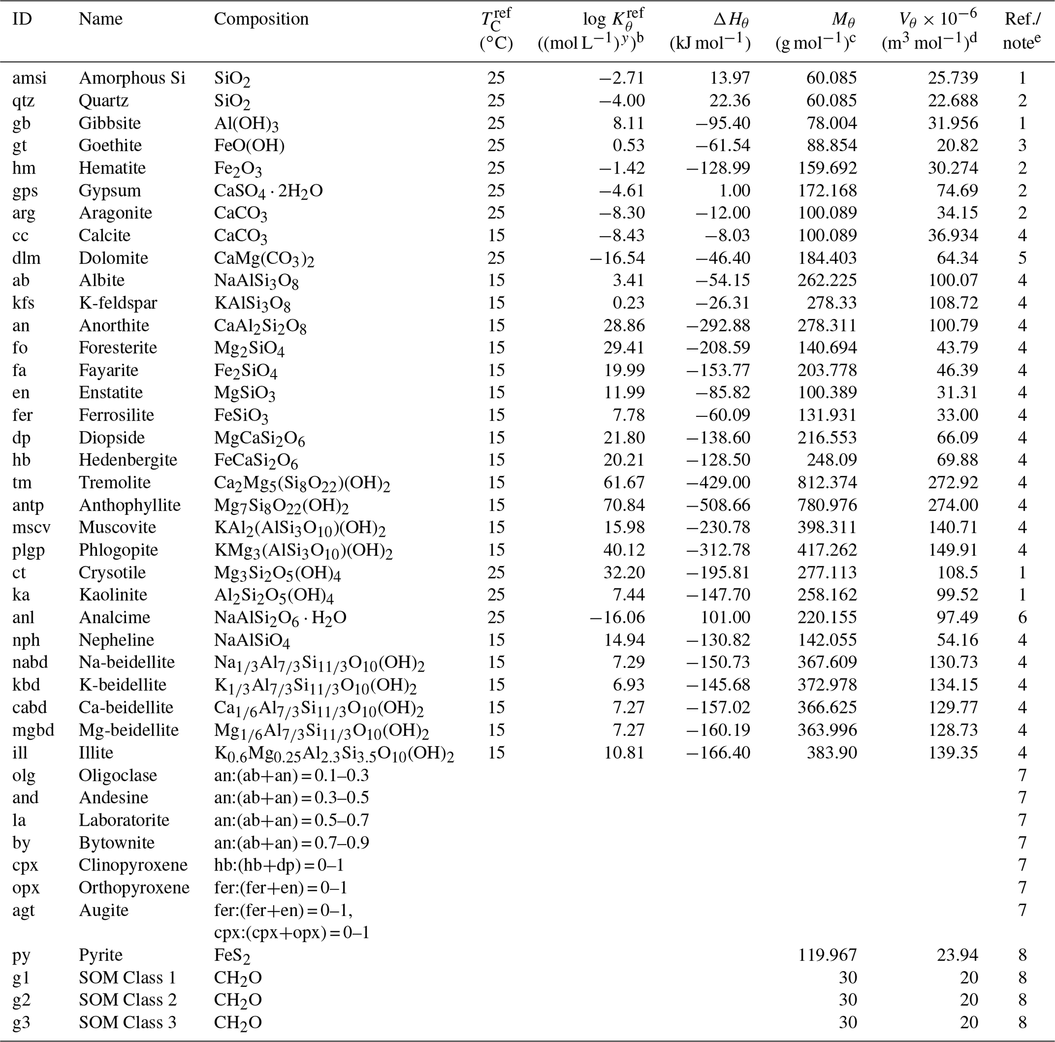
a The thermodynamic constant for species θ (Kθ) is calculated as exp[−ΔHθ{ 1/(], where TC is temperature in ∘C and ℜ is the gas constant in units of kJ mol−1 K−1 ( kJ mol−1 K−1). Thermodynamic constants for SOMs and pyrite are not defined here as the saturation states for these species are kinetically defined (see Sect. 2.2.2 for more details): (pyrite) and ) (SOM Classes 1 to 3), where is the partial pressure of soil O2 (atm) and is the Michaelis constant for aerobic respiration (0.121 atm; see Kanzaki and Kump, 2017, and references therein). b Units change with y depending on minerals. c From Robie et al. (1978) except for illite and beidellites (Wolery and Jove-Colon, 2004), hedenbergite (calculated from the molar weight and density in https://www.mindat.org, last access: 15 June 2022) and SOMs (Mayer et al., 2004). Solid solutions are calculated from molar volumes of endmember minerals. d From Robie et al. (1978). When not available in Robie et al. (1978), calculated from chemical composition. e (1) From phreeqc.dat available in PHREEQC v.3 (Parkhurst and Appelo, 2013). (2) From minteq.v4.dat available in PHREEQC v.3 (Parkhurst and Appelo, 2013). (3) Data by Sugimori et al. (2012) from the Lawrence Livermore National Laboratory thermodynamic dataset, thermo.com.v8r6+.dat (Delany and Lundeen, 1990). (4) Summarized data by Kanzaki and Murakami (2018) from thermo.com.v8r6+.dat (Delany and Lundeen, 1990). (5) Data for disordered dolomite from minteq.v4.dat available in PHREEQC v.3 (Parkhurst and Appelo, 2013). (6) Wilkin and Barnes (1998). (7) Calculated assuming an ideal solid solution after Gislason and Arnorsson (1993). (8) Not defined (see caption a and Sect. 2.2.2).
Table 2Dissolution/precipitation kinetic data of solid speciesa.
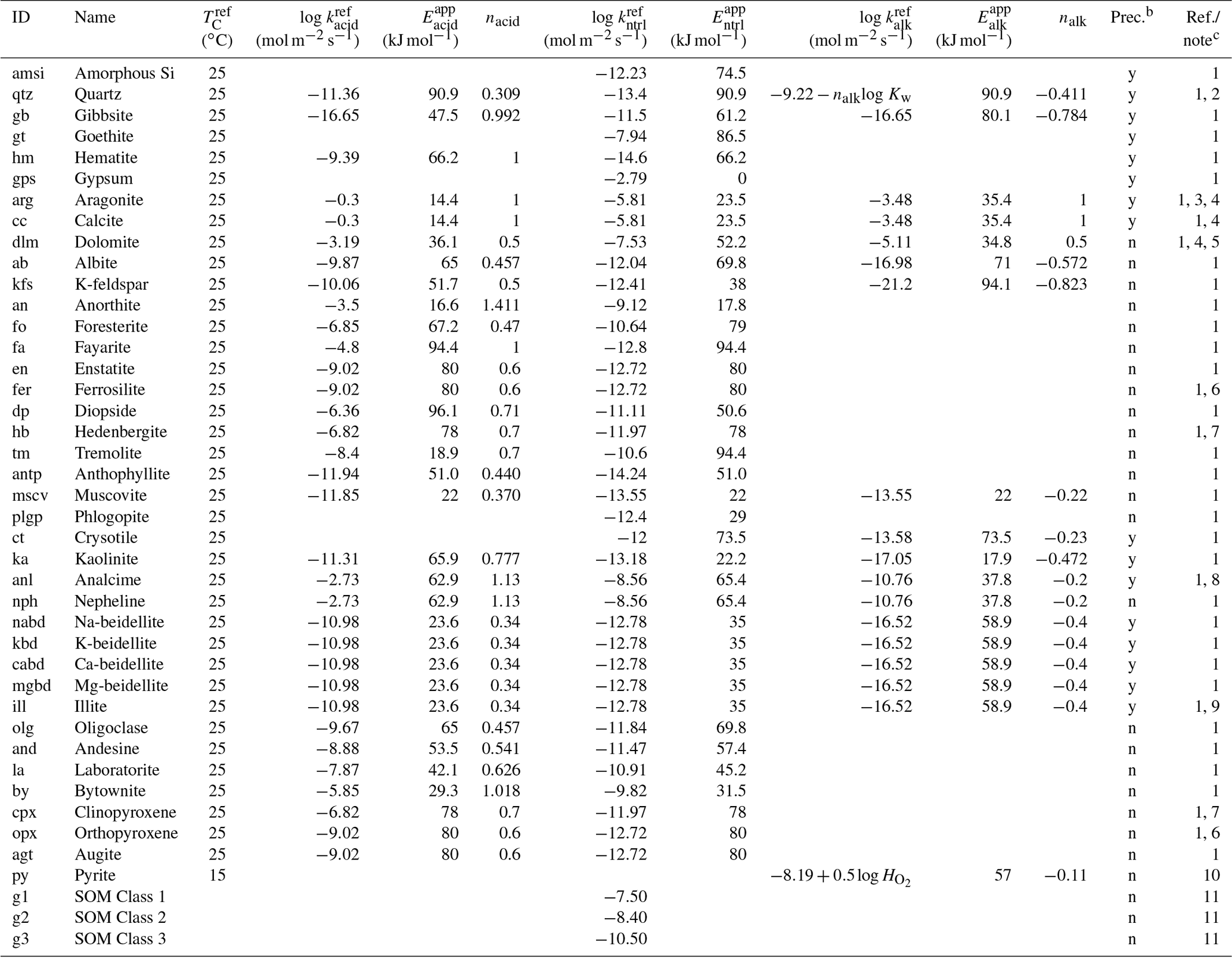
a The rate constant for species θ (mol m−2 s−1) is calculated as kθ= [Hexp[ 1/(exp[ 1/( [Hexp[ 1/(TC+273.15) -1/( /ℜ], where TC is temperature in ∘C and ℜ is the gas constant in units of kJ mol−1 K−1 ( kJ mol−1 K−1), except for carbonates and SOMs. For carbonates, [H+] in the last term of the above equation (“base” mechanism) needs to be replaced by (atm), the partial pressure of soil CO2 (“carbonate” mechanism) according to Palandri and Kharaka (2004), and for SOMs, rate constants are assumed to be independent of pH and temperature. b Solid species that are unlikely to precipitate are not allowed to precipitate even when porewater is supersaturated with respect to them in the model, denoted with “n” in this column. Those that can precipitate are denoted with “y”. c (1) Palandri and Kharaka (2004). (2) “Acid” and “base” mechanisms from Brantley et al. (2008) (Kw is the water dissociation constant) and the “neutral” mechanism from Palandri and Kharaka (2004). Activation energy for the “neutral” mechanism is assumed to be applicable to other mechanisms. (3) Data for calcite are assumed. (4) The “base” mechanism is replaced by the “carbonate” mechanism (see caption a for details). (5) Data for disordered dolomite are assumed. (6) Data for enstatite are assumed. (7) Data for augite are assumed. (8) Data for nepheline are assumed (cf. Ragnarsdóttir, 1993). (9) Data for smectite are assumed (cf. Bibi et al., 2011). (10) is the solubility of O2 (mol L−1 atm−1). Dependences on pH and O2 are from Williamson and Rimstidt (1994) and apparent activation energy from McKibben and Barnes (1986). (11) See caption a. Corresponding to turnover times of 1, 8 and 1000 years for decomposition of SOM Classes 1, 2 and 3, respectively (cf. Chen et al., 2010).
2.1 Overview
The basic framework of SCEPTER is derived from previous models designed to simulate reactive transport and weathering in natural soil systems, with a focus on pyrite and organic matter oxidation (Kanzaki and Kump, 2017) and silicate mineral transformation (Kanzaki et al., 2020). SCEPTER can currently simulate up to 39 minerals and different classes of soil organic matter (SOM; currently configured with three classes), 10 independent aqueous species along with 48 dependent aqueous species, and 4 independent gas species (Tables 1–5). Reaction kinetics, especially dissolution/precipitation, are explicitly implemented for individual solid species and are fully coupled with the temporal and spatial evolution of aqueous and gas species (e.g., Table 2). One can further add/remove a series of additional reactions to the system associated with solid, aqueous, and/or gaseous species (referred to as “extra” reactions, e.g., Table 6). Particular features of SCEPTER designed to interrogate ERW in terrestrial soil systems include (1) implementation of bio-mixing in the upper soil layers using a transition matrix approach, (2) time-dependent application of crushed rock feedstock to the soil surface, (3) options for time-varying boundary conditions including porosity and advection rates of solids and porewater, and (4) a range of user options for calculation and specification of the surface area of solid species. These features of the model are specifically designed for aiding in robust prediction of enhanced weathering on terrestrial ecosystems, including croplands and hinterlands (e.g., Hartmann et al., 2013; Taylor et al., 2016; Beerling et al., 2020; Goll et al., 2021).
In the following we describe the theoretical framework of the model (Sect. 2.2), its numerical implementation (Sect. 2.3), and the user input in relation to model initialization and boundary conditions (Sect. 2.4). The model code is written in Fortran90 (see the code availability section).
Table 3Thermodynamic data for aqueous speciesa.
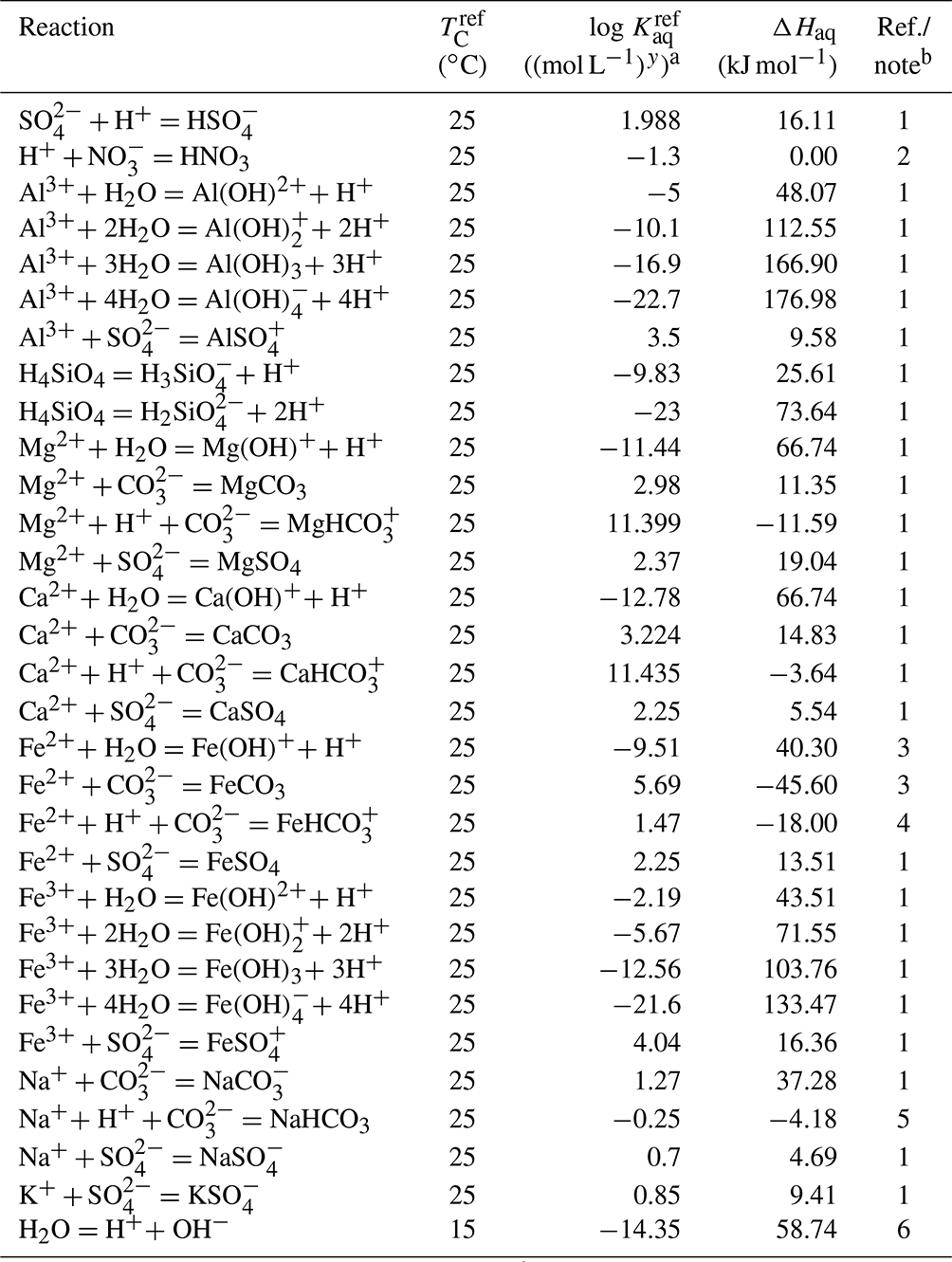
a Thermodynamic constant (Kaq) is calculated as , where TC is temperature in ∘C and ℜ is the gas constant in units of kJ mol−1 K−1 ( kJ mol−1 K−1). b (1) From phreeqc.dat available in PHREEQC v.3 (Parkhurst and Appelo, 2013). (2) Maggi et al. (2008). Temperature dependence is assumed to be 0. (3) Kanzaki and Murakami (2016). (4) Thermodynamic constant for Fe from Kanzaki and Murakami (2016) divided by that for (Table 4). (5) Thermodynamic constant for Na NaHCO3 from phreeqc.dat available in PHREEQC v.3 (Parkhurst and Appelo, 2013) divided by that for H (Table 4). (6) Kanzaki and Murakami (2015).
Table 4Thermodynamic data for gaseous speciesa.
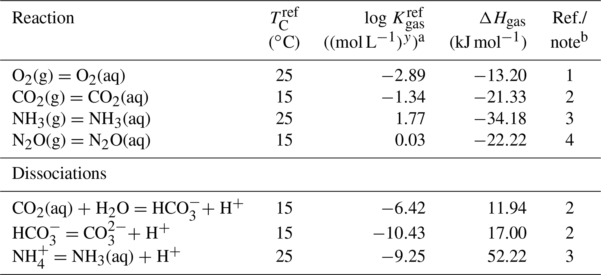
a The thermodynamic constant (Kgas) is calculated as , where TC is temperature in ∘C and ℜ is the gas constant in kJ mol−1 K−1 ( kJ mol−1 K−1). b (1) Kanzaki and Murakami (2016). (2) Kanzaki and Murakami (2015). (3) From wateq4f.dat available in PHREEQC v.3 (Parkhurst and Appelo, 2013). (4) Weiss and Price (1980).
2.2 Theoretical framework
2.2.1 Tracing solid, aqueous and gas species in soils
SCEPTER is based on previous models designed to represent fundamental aspects of natural weathering (e.g., Bolton et al., 2006; Brantley and Lebedeva, 2011; Li et al., 2014; Steefel et al., 2015; Kanzaki et al., 2020). Solid minerals are transported upward by continental uplift and eroded at the surface while reacting with solutes in porewater whose transport is dominated by molecular diffusion plus advection caused by downward infiltration. Some solutes are derived from the gas phase present in soil pore space whose composition is controlled by diffusive transport plus consumption/production through reactions within soil, including dissolution into and degassing from porewater. These reactions and transport of solid, aqueous and gaseous phases are simulated within a 1D model soil domain where materials are exchangeable at the top and bottom boundaries.
In addition to the above basic description of the model's framework as a natural soil/rock weathering simulator, SCEPTER implements bio-mixing of solid particles in soils and a rain of solid particles onto the soil surface (Sect. 2.1). Including these additional supply and mixing effects, a solid species θ is simulated according to the following generalized equation (cf. Boudreau, 1997; Kanzaki et al., 2020, 2021):
where mθ is the mole amount of solid species θ per unit bulk soil/rock volume (mol m−3), t is time (yr), z is the depth of the weathering profile (m), w is the advection rate of solid phases (m yr−1), Rθ and Jθ are the net dissolution and rain rates of solid species θ, respectively (mol m−3 yr−1), Rκ denotes the rate of the κth extra reaction (mol m−3 yr−1) whose stoichiometry with respect to consumption of θ is defined by γκ,θ, nxrxn is the total number of extra reactions, Eθ (z, z′) is the rate of particle transfer between locations at z and z′ by bio-mixing (m−1 yr−1) and zml is the mixed layer depth (m) within which bio-mixing occurs. The exchange function Eθ (z, z′) expresses the bio-mixing rate in a generalized continuous form, whose discretized counterpart can be formulated with a transition matrix (e.g., Boudreau, 1997; Shull, 2001; Kanzaki et al., 2021). Various bio-mixing styles and corresponding transition matrices are elaborated in Sect. 2.2.5. As described above, SCEPTER also allows flexible addition of many additional reactions (with example “extra” reactions given in Table 6 and discussed in Sect. 2.2.2) beyond those parameterized with the thermodynamic and kinetic constants in Tables 1 and 2. See the following subsections for more details on individual transport and reaction terms.
Table 5Diffusion coefficient for aqueous and gaseous speciesa.

a The diffusion coefficient is calculated as , where TC is temperature in ∘C and ℜ is the gas constant in units of kJ mol−1 K−1 ( kJ mol−1 K−1), except for NH3 gas. A power function of temperature is assumed for NH3 gas from Massman (1998): D=624{ (TC+273.15)/273.15}1.81 (m2 yr−1). b (1) From Li and Gregory (1974). (2) From Rebreanu et al. (2008). (3) Kanzaki and Murakami (2016). (4) A value of 0.14 cm2 s−1 is assumed (e.g., Pritchard and Currie, 1982), and apparent activation energy is assumed to be the same as that for O2 gas. (5) Massman (1998). See caption a. (6) Assumed to be the same as CO2 diffusion (e.g., Pritchard and Currie, 1982). (7) The diffusion coefficient of is assumed to be the same as that of aqueous CO2. (8) diffusion from Schulz and Zabel (2006). (9) From Schulz and Zabel (2006).
Table 6Extra reactions and their kinetic laws.
a Given in units of mol m−3 yr−1. b (1) Singer and Stumm (1970). (2) After Maggi et al. (2008). A linear pH function is fitted to an exponential function.
When an element with a given redox state dissolves in porewater and is not sourced from the soil atmosphere, the element is regarded as an aqueous species in the model. The total amount of all dissolved forms of the element per unit porewater volume is traced as an independent variable for modeling solutes in porewater. Specific chemical forms (e.g., hydrolyzed forms and complexes with other ions) are assumed to be in equilibrium, and their concentrations are calculated based on the tracked total concentrations of individual dissolved elements and thermodynamics of association/dissociation reactions (Table 3, Sect. 2.2.2). For each dissolved element, all associated chemical forms are assumed to be transported uniformly (i.e., the same diffusion coefficients are applied to various aqueous forms of a dissolved element; Table 5, Sect. 2.2.4), and thus the governing equation for a dissolved element is given as follows:
where cς is the porewater concentration of dissolved element ς (mol L−1), ϕ is the porosity, σ is the water saturation ratio, ℓ is a unit conversion factor (103 L m−3), v is the porewater advection rate (m yr−1), τaq is the tortuosity factor for solute diffusion in porewater, Dς is the diffusion coefficient of dissolved element ς (m2 yr−1), nsld is the total number of simulated solid species, γθ,ς is the mole amount of ς released upon dissolution of 1 mole of mineral θ and γκ,ς is the stoichiometry of ς production in the κth extra reaction.
A gas species is introduced into the model when it is produced/consumed by aqueous and/or solid species. In the current version of SCEPTER, soil CO2, O2, NH3 and N2O can be included as gas species. The independent variable is taken to be the soil partial pressure for a given gas species, and concentrations of all dissolved forms derived from the gas species are taken to be dependent variables. Transport occurs via diffusion for a gas species and via diffusion plus porewater advection for its dependent dissolved forms (Sect. 2.1). The governing equation for a gas species is accordingly given by
where pε is the partial pressure of soil gas ε (atm), γθ,ε is the mole amount of ε released upon dissolution of 1 mole of solid species θ, Hε is the total solubility of ε (mol L−1 atm−1) and γκ,ε is the stoichiometry of ε production in the κth extra reaction. In Eq. (3), αε and are the unit conversion factor (mol m−3 atm−1) and effective diffusion coefficient (mol atm−1 m−1 yr−1) for soil gas ε, respectively, to include the reactive transport of dependent dissolved forms of ε (e.g., Elberling and Nicholson, 1996):
where η is the unit conversion from atm to molarity (, where ℜ is the gas constant, 0.08205 L atm mol−1 K−1, and T is the temperature in K), τgas is the tortuosity factor for gas diffusion in pore air space and and are the diffusion coefficients (m2 yr−1) for the gas and aqueous phases of ε, respectively. Individual reaction and transport terms are discussed below.
2.2.2 Reactions
Dissolution/precipitation of a solid species θ (Rθ) is formulated as a function of the saturation state of the species in porewater (Ωθ), rate coefficient (kθ, mol m−2 yr−1) and surface area of the species per unit bulk soil/rock volume available to porewater (Sθ, m2 m−3):
Here, kθ is a function of porewater pH and soil CO2 (for carbonates) according to Palandri and Kharaka (2004) (Table 2), and Sθ is related to mθ, with a number of potential scaling options (see Sect. 2.2.6). The saturation state Ωθ is calculated based on thermodynamic data for solid species (Table 1). When decomposition of solid species occurs as a redox reaction, e.g., pyrite oxidation and SOM decomposition, Ωθ is defined kinetically. For instance, pyrite oxidation proceeds according to, e.g., Williamson and Rimstidt (1994):
where is the partial pressure of soil O2 (atm). We conventionally define the saturation state for pyrite (Ωpy) as
so that Eq. (6) can be applied to all solid species (Tables 1 and 2). In addition to the dissolution/precipitation reactions specific to individual solid species, one can add extra reactions to the system whose kinetics are explicitly considered. Currently implemented extra reactions and their kinetic laws are listed in Table 6.
All dependent aqueous species are calculated assuming that they are in equilibrium and satisfy the mass balance and charge balance in porewater at any model time step and at all model depths (cf. Steefel et al., 2015). Generally, the mass balance for dependent aqueous species derived from a given dissolved element is given as
where is the porewater concentration of the ith dependent aqueous species derived from dissolved element ς (mol L−1) and nς is the total number of dependent aqueous species of ς. Note that the current version of the model does not include any polymers (e.g., Si2O(OH)6), as aqueous species and thus 1 mole of dependent aqueous species of dissolved element ς contains 1 mole of ς as assumed in Eq. (9). We define the first dependent species of a given dissolved element as the free dissolved form, except for Si, whose first dependent species is defined as H4SiO4, and the other species as products formed via reactions of the first dependent species with other aqueous species in porewater, given, respectively, by
where Kς,i is the thermodynamic constant for production of the ith dependent aqueous species of dissolved element ς, [H+] is the porewater H+ concentration (mol L−1), , and are the stoichiometry of H+, dissolved element ς′ and gas species ε, respectively, in the reaction that produces the ith dependent aqueous species of ς, and naq and ngas are the total numbers of independent aqueous and gas species, respectively.
Any aqueous species derived from a gas species is also assumed to be in equilibrium with the gas in soil pore space:
where is the porewater concentration of the jth dependent aqueous species derived from soil gas ε (mol L−1), KH,ε is Henry's constant for soil gas ε (mol L−1 atm−1), Kε,j is the thermodynamic constant for production of jth dependent aqueous species of ε, and and are the stoichiometry of H+ and the dissolved element ς, respectively, in the reaction that produces the jth dependent aqueous species of ε. The total solubility of ε (Hε, Eq. 3) is then given by
Finally, porewater pH is obtained based on charge balance:
where and are the charges of the ith and jth dependent aqueous species derived from aqueous species ς and gas species ε, respectively, and [OH−] is the porewater OH− concentration (mol L−1). Note that double counting of dependent aqueous species is avoided in Eq. (14). Porewater concentrations of H+ and OH− are related to one another via the thermodynamic constant of water dissociation Kw (mol2 L−2):
Once pε and cς are known, Eqs. (9)–(15) can be solved to obtain porewater concentrations of all dependent aqueous species including [H+] or pH.
2.2.3 Porosity and advection of solids and porewater
The temporal and spatial evolution of porosity is calculated based on Eq. (1) and the constraint of volume conservation:
where Vθ is the molar volume of solid species θ (m3 mol−1) (Table 1). Summing Eq. (1) (multiplied by Vθ for all the considered solid species in the model) and using Eq. (16) yields
To satisfy the volume conservation (Eq. 16), porosity (ϕ) and advection rate (w) are calculated simultaneously by Eq. (17) assuming a scaling relationship. In the default setting, w is assumed to be constant and independent of ϕ, but two other user options are available in which wϕ or w(1−ϕ) can be assumed to be constant (cf. Wang et al., 2014; Chen et al., 2020).
Advection of porewater is assumed to be caused by steady-state porewater flow (e.g., Stonestrom et al., 1998). Thus, advection terms for aqueous species (the first terms on the right-hand side of Eqs. 2 and 3) are calculated based on a net water flux to the soil system, q (m yr−1), and a water saturation profile (σ):
By default, SCEPTER fixes the profiles of q and σ, but these can be changed along model time as a user option. The depth profile of σ is assumed to increase linearly from the surface level to the water table, where σ=1, and is thus controlled by two variables – the value of σ at the surface and the depth of the water table (cf. Sect. 2.4; Kanzaki et al., 2020).
2.2.4 Diffusion
Molecular diffusion becomes slower in porous media because of tortuosity (Clennell, 1997). The tortuosities of pore air- and water-filled spaces are represented by factors τgas and τaq, both of which are parameterized with porosity and water content in soils according to Aachib et al. (2004):
See Table 5 for the molecular diffusion coefficients for gas and aqueous species where tortuosity factors are not accounted for.
2.2.5 Bio-mixing
SCEPTER parameterizes various styles of soil mixing (bio-mixing) within a transition matrix framework. Here, we provide a short description of the transition matrix framework for parameterization of bio-mixing. For more details, the reader is referred to, e.g., Boudreau (1997), Shull (2001) and Kanzaki et al. (2021).
The particle transport rate for solid species θ from layer i to layer j is defined here as Pθ,ij (yr−1), given by
where Nθ,ij is the number of particles of species θ moved from layer i to layer j, nml is the total number of layers within the bio-mixed zone and τ is the time (yr) required for the particle displacements. Note that the particle transport probability, given as , corresponds to components at (i, j) of the transition matrix (Trauth, 1998; Shull, 2001). The time rate of change in soil concentration of solid species θ at layer i caused by bio-mixing ([]mix) can then be described with Pθ,ij:
where mθ,i is the concentration of θ (mol m−3) at soil layer i and δzi is the thickness of layer i (m) (see Kanzaki et al., 2021, for a more detailed derivation). To simplify Eq. (22), a modified transition matrix for species θ is introduced, whose components at (i, j) are denoted as Kθ,ij and calculated based on the particle transport rate Pθ,ij:
From Eqs. (22) and (23), we obtain
Equation (24) can be regarded as the discretized form of the bio-mixing term shown in Eq. (1).
SCEPTER can implement a range of different transition matrices for parameterizing different soil mixing regimes, including Fickian mixing (e.g., bulk bioturbation), homogeneous mixing (e.g., deep rotary tilling prior to sowing row crops), inversion tilling, or particle-tracking automata-based simulators (see Boudreau et al., 2001; Choi et al., 2002; Kanzaki et al., 2019). Simulations shown here implement either Fickian or homogeneous mixing (see below). The transition matrix for Fickian bioturbation (parameterized with a biodiffusion coefficient Db, Goldberg and Koide, 1962) can be expressed by
where Db,i represents the biodiffusion coefficient at soil layer i. SCEPTER adopts a depth-independent coefficient by default: m2 yr−1 (cf. Jarvis et al., 2010; Astete et al., 2016).
The transition matrix for homogeneous mixing is given by
where Ph (yr−1) is the homogeneous transport rate of solid particles between soil layers. The model assumes Ph=0.01 yr−1 as the default parameterization (cf. Kanzaki et al., 2021).
2.2.6 Surface area
Surface areas of solid species θ available for reaction with porewater (Sθ) significantly impact dissolution/precipitation rates of solid phases (Eq. 6), and thus the parameterization of surface area is of critical importance for predicting the behavior of elements in soils. However, there are significant differences in the parameterization of Sθ between models (e.g., Bolton et al., 2006; Steefel, 2009; Li et al., 2014) and/or between solid species (e.g., minerals vs. SOM; e.g., Jia et al., 2021). SCEPTER provides multiple options for parameterization of Sθ.
(1) Surface area parameterization based on hydraulic radius
The hydraulic radius of a given porous medium (rH, m) can be defined as the ratio of pore volume against pore surface area (Fanchi, 2018). Conceptually, the value of rH can be thought of as the average effective radius of particles within a weathering/soil system. In this formulation, the overall surface area of pores in a unit bulk soil/rock volume can be described as (m2 m−3). The area available for mineral-phase θ can then be calculated as the product of the soil volume fraction of mineral θ and , i.e.,
Equation (27) is specified as the default option in SCEPTER, following Kanzaki and Kump (2017) and Kanzaki et al. (2020). A linear relationship between Sθ and mθ as in Eq. (27) is also widely assumed in other models that calculate the surface area based on measured specific surface area (m2 g−1), soil concentration (mol m−3) and molar weight (g mol−1) of minerals (see (4) below; Brantley and Lebedeva, 2011; Li et al., 2014).
However, several other reactive-transport models assume that the pore surface area available to mineral θ is not directly proportional to its volume fraction mθVθ but is instead proportional to ( with an intension to convert volume fraction to surface area fraction (e.g., Steefel, 2009; see also Bolton et al., 2006, who implemented a similar dependence with a shrinking particle model). To realize this Sθ–mθ relation, SCEPTER can also adopt an alternative function for Sθ:
In Eq. (28), the hydraulic radius rH is still used to specify the total surface area available to minerals.
With the options presented above (Eqs. 27 and 28), surface area normalized to porosity and mineral fraction (i.e., ) does not change with time or depth. To enable evolving surface area while using only average effective radius of particles, SCEPTER adopts two optional scaling relationships between surface area and porosity (e.g., Emmanuel and Berkowitz, 2005):
Equation (29) is adopted as the default option in the current version of SCEPTER.
(2) Parameterization based on particle size distribution
The surface area of a porous medium can be explicitly calculated if the shapes of component particles and the particle size distribution (PSD) are known, assuming that aggregation of particles does not reduce the surface area available to porewater (which can occur in natural systems depending on the assumed particle shapes). Tracking the PSD can be facilitated by adopting a shrinking particle model in which all particles maintain their shapes as their volumes change with ongoing dissolution/precipitation (e.g., Nicholson et al., 1990; Safari et al., 2009). For a batch solution system in which minerals only dissolve without being transported, surface area can be calculated relatively easily in a shrinking particle framework (e.g., LeBlanc and Fogler, 1987). For example, Beerling et al. (2020) adopted a shrinking particle model to calculate the particle size distribution and particle surface area in their “performance” simulations of basalt powder application onto croplands assuming a uniform spherical shape. The problem becomes more complex with solid-phase transport (e.g., in 1-D), where solid phases not only precipitate/dissolve but are also added at the top of the model domain and transported vertically (e.g., Eq. 1). To facilitate inter-model comparison and to add flexibility for representing reactive surface area, SCEPTER contains a numerical scheme and corresponding subroutine for explicit PSD tracking within a shrinking particle framework. The essential framework is provided below, while numerical implementation is detailed in Sect. 2.3.
Particles are all assumed to be spherical (e.g., Beerling et al., 2020) and chemically and mineralogically homogeneous regardless of the size. A shrinking particle scheme is then applied where net dissolution/precipitation occurs within soils. First, SCEPTER defines the PSD as f(r, t, z) – the number of particles per unit bulk soil volume for a given radius bin as a function of radius r, time t and soil depth z. Applying the general equation for solid species to f(r, t, z) yields
where [∂f(r, t, z)/∂t]diss is the time rate of change in f(r, t, z) caused by net dissolution and [∂f(r, t, z)/∂t]rain is the supply rate of particles at the soil surface with a specified PSD, which satisfies the following:
Shifts in the particle size distribution caused by net dissolution/precipitation ([∂f(r, t, z)/∂t]diss) can be formulated with a population balance equation (e.g., LeBlanc and Fogler, 1987; Iggland and Mazzotti, 2012):
where g(r, t, z) is the particle growth rate (m yr−1). Within a shrinking particle framework, the particle growth rate is specified as (e.g., LeBlanc and Fogler, 1988; Safari et al., 2009)
Here, k′ is the particle dissolution rate in units of m yr−1. Loss of particles is allowed at the lower boundary, i.e., particles are assumed to be completely dissolved when r becomes smaller than the minimum radius considered in the model. Also, when dissolution (imposed by Eq. 32) is intense enough to consume all existing particles, particles are allowed to be lost. Meanwhile, particles are not allowed to grow over the maximum radius set by the model. At each time step, Eqs. (32), (34) and (35) are solved at once to obtain the values for [∂f(r, t, z)/∂t]diss that satisfy the volume balance (Sect. 2.3).
Given a PSD for particles applied at the soil surface, defined here as frain(r) that is only a function of radius but not of time or depth, one can obtain a function krain(r, t, z) in units of yr−1 satisfying Eq. (33) and the following:
By solving Eqs. (31)–(36), one can obtain the full PSD reflecting both shrinking particles via net precipitation/dissolution and addition/transport of particles. The above scheme generally satisfies the volume balance:
The total surface area is then calculated based on the PSD as follows:
Here, the total pore surface area per unit soil/rock volume is again represented by the hydraulic radius rH to facilitate comparison with the default surface area calculation where rH is directly specified as the average effective radius of particles (see (1) above). The surface areas for individual solid species (Sθ) can then be calculated by either Eq. (27) (the default in SCEPTER) or (28). When adopting the PSD-based formulation, the surface area evolves temporally and spatially in a dynamic fashion without any further parameterization.
(3) Surface roughness
Mineral surfaces are not necessarily smooth and can have complicated geometry and resultant surface roughness that increases the surface area per unit volume/mass (e.g., White and Peterson, 1990). One can introduce a roughness factor λ to correct the surface area calculated for a smooth geometry of solid particles with an assumed shape. This additional parameterization is especially useful when one considers a particle size distribution based on ideal shapes ((2) above). The roughness factor is calculated assuming a dependency on particle size following Beerling et al. (2020) (cf. Navarre-Sitchler and Brantley, 2007):
As a user option, one can include λ in the PSD calculation method in (2); in this case, the k′ and r2 terms in Eqs. (35) and (38) are replaced with λk′ and λr2, respectively.
Implementation of a roughness factor is of limited use for formulations that calculate surface area directly from hydraulic radius (Eqs. 27–30), because the hydraulic radius should in principle already account for roughness in the pore surface. As a result, in the default surface area calculation (Eqs. 27 and 29), a roughness factor is not included, although SCEPTER contains a user option to add a roughness term to Eqs. (27)–(30).
(4) Specific surface area of solid species
The options for calculating surface area in SCEPTER described above are based on the total surface area of pores and the fractions of individual solid species in soils. These approaches all assume that every patch of pore surface is mineralogically and chemically homogeneous. However, individual solid species can have unique particle size distributions and thus specific surface areas that are different from the surface areas of the bulk soil multiplied by solid species fractions. Based on the concept of specific surface areas for individual solid species, SCEPTER includes an additional user option that enables the surface area calculation for individual solid species.
Defining the specific surface area of solid species θ as Aθ (m2 g−1), the surface area of θ available to porewater (Sθ, m2 m−3) can alternatively be represented by (e.g., Brantley and Lebedeva, 2011; Li et al., 2014)
where Mθ (g mol−1) is the molar weight of solid species θ (Table 1). To facilitate comparison with the surface area parameterization using a hydraulic radius (Eq. 27), we introduce an apparent hydraulic radius for solid species θ as rH,θ (m):
where ρθ (g m−3) is the particle density of solid species θ and . The apparent hydraulic radius rH,θ (m) can be thought of as the average effective radius of particles which are composed solely of solid species θ. SCEPTER has the option of calculating individual surface areas according to Eqs. (40) and (41), with a specified rH,θ the evolution of which can be further specified by replacing rH with rH,θ in Eq. (29) or (30).
SCEPTER can evaluate specific surface areas for individual solid phases by tracking PSDs for individual species. The scheme introduced in (2) still holds, but in this case the PSD is defined and calculated for individual solid species. Defining the PSD and particle growth and dissolution rates for solid species θ as fθ(r, t, z), gθ(r, t, z) and , respectively, the equations to solve PSD for bulk soil, i.e., Eqs. (31)–(38), can be used to solve fθ(r, t, z) by replacing f(r, t, z), g(r, t, z) and k′ with fθ(r, t, z), gθ(r, t, z) and , respectively, and dropping summation symbols and notations (i.e., replacing ), and with ), VθJθ and mθVθ, respectively). Then, the specific surface area for solid species θ can be calculated as
and the corresponding apparent hydraulic radius can be evaluated as
The roughness factor λ can further be included by replacing and r2 with and λr2, respectively, as described for the PSD calculation for bulk soil ((3) above). For instance, ground minerals have been characterized by significant surface roughness based on measured surface areas that are larger than expected from their grain sizes (e.g., Brantley and Mellot, 2000; Renforth, 2012; Renforth et al., 2015).
(5) Reactions not limited by surface area
Decomposition of some solid species can proceed without being affected by the surface area available to porewater. In the current version of SCEPTER, three classes of SOM are assumed to decay depending on their concentrations but independently of their surface areas (e.g., Jia et al., 2021):
For all the other solid species, their dissolution/precipitation kinetics are assumed to be dependent on the surface areas which are calculated based on rH or rH,θ, either directly specified by the user or calculated from tracked PSD(s), as described above.
Table 7Boundary conditions for example simulations.

a Only IDs of solid species and extra reactions are denoted (Tables 1 and 6). b Composition of dust is assumed to be the basalt composition by Beerling et al. (2020). cN is the number of grid points, ztot is the bottom depth of simulated soil, zsat is the depth of the water table, σ0 is the surface water saturation ratio and ϕ0 is the initial porosity. d When surface area is calculated based on tracked particle size distributions, “PSD” is denoted. e (1) Rainwater composition is assumed to be that of pure water saturated with respect to atmospheric CO2 and O2. (2) Atmospheric CO2 and O2 are assumed to be and 0.21 atm, respectively. (3) Parent rock concentrations of albite and kaolinite are 10 and 10−3 wt %, respectively. (4) Parent rock concentrations of pyrite and goethite are 0.56 and 10−3 wt %, respectively. (5) Parent rock concentrations of solid species are from those for Site 1 in Table 8. (6) Abiotic weathering, biotic weathering and basalt application experiments in Figs. 3, 4 and 6–9 are repeated with surface area parameterization based on tracked particle size distributions for bulk soil (Fig. 10). The same basalt application experiment was conducted except with tracking PSDs for individual solid species and calculating corresponding specific surface areas (Figs. 11 and 12).

Figure 1Simulation of abiotic weathering of albite. Soil concentrations, saturation states and dissolution/precipitation rates of solid species are plotted in panels (a)–(c), respectively; porewater concentrations of aqueous species and pH in (d) and (e), respectively; soil porosity and particle density in (f) and (g), respectively; ratio of total volume of solid species against solid space specified with porosity in (h). See Table 7 for the details on the boundary conditions of the simulation.
2.3 Numerical implementation
Initialization of SCEPTER involves loading input data, including chosen species to be simulated, and initial and boundary conditions (see Sect. 2.4). In the case of a restart experiment from a previous simulation, initial conditions are overwritten with the results from the previous (restart) experiment. After initialization, SCEPTER begins time integration of the governing equations (see Sect. 2.2). For a given time step, the boundary conditions and time step duration can be modified if the user selects time-varying changes to water flux, temperature, particle rain rate or water saturation ratio. Time step duration also evolves adaptively depending on the time to convergence in the previous integration step (from 10−18 up to 103 years). Kinetic and thermodynamic constants are then updated, and the concentrations of all chosen species are solved via Newton–Raphson iteration in a fully coupled way (see below). Finally, porosity, surface area and advection rate(s) of solid phases are updated. By default, SCEPTER updates porosity, surface area and advection rates iteratively at each time step as verified by porosity convergence, but there is also a user option to bypass the porosity iteration and simply update porosity, surface area and advection rate(s) once per time step. The latter option is computationally less expensive and will yield the same solutions when the time step duration is relatively small. The default criterion for numerical convergence is a solution difference of (mol m−3 or m3 m−3) from the previous iteration in each time-integration step (cf. Steefel, 2009).
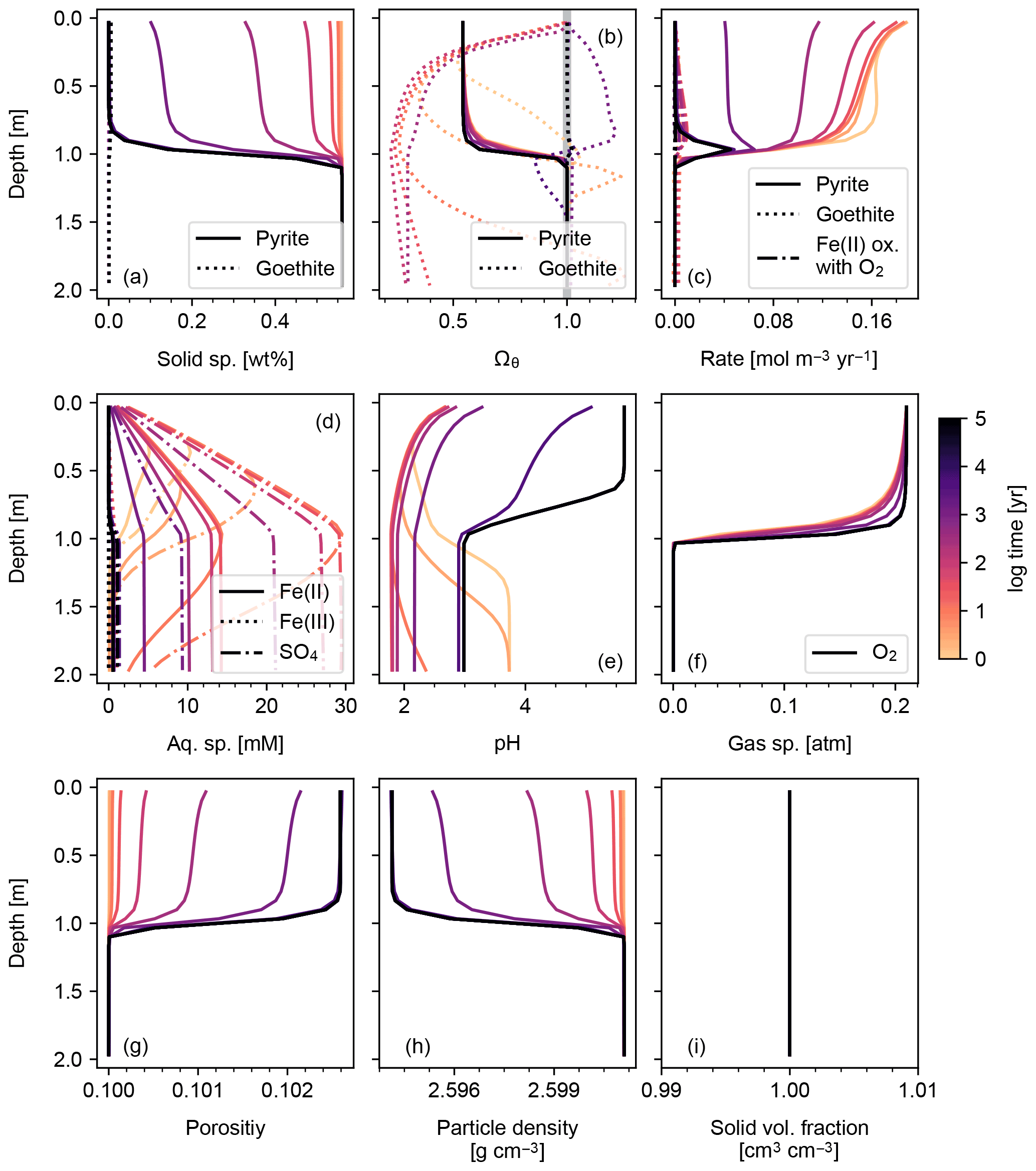
Figure 2Simulation of abiotic weathering of pyrite. Soil concentrations and saturation states of solid species are plotted in (a) and (b), respectively; rate profile of reactions within soil in (c); porewater concentrations of aqueous species and pH in (d) and (e), respectively; concentrations of soil gases in (f); soil porosity and particle density in (g) and (h), respectively; ratio of the total volume of solid species against solid space specified with porosity in (i). See Table 7 for details on the boundary conditions of the simulation.
The governing equations of SCEPTER are differentiated via a finite-difference method. First-order upwind and second-order central differencing schemes are applied to advection and diffusion terms, respectively (Eqs. 1–3). Equation (24) is used as a difference form of the bio-mixing term in Eq. (1). Time derivatives (left-hand side of Eqs. 1–3) are discretized in accordance with a backward Euler scheme. The finite-difference expressions are then solved via a fully coupled Newton–Raphson method (Steefel and Lasaga, 1994). Parent rock values are enforced below the bottom of the model domain as a boundary condition for solid species. For aqueous and gas species, the bottom of the model domain is assumed to be impermeable with respect to molecular diffusion (i.e., zero concentration gradient), while the compositions of rainwater and the overlying atmosphere are enforced as boundary conditions at the top of the model domain on dissolved and gaseous species, respectively. When there is no user input, a value of 10−20 mol m−3 or mol L−1 is assumed for the boundary parent-rock or rainwater concentration, respectively, and 0.21, 10−3.5, 10−9 and atm for atmospheric O2, CO2, NH3 and N2O, respectively. Concentrations of all dependent aqueous species as well as associated rate constants are always updated (Sect. 2.2.2, Tables 1–4), including during Newton–Raphson iteration.
The calculations of porosity and advection rate of solid species are conducted by differentiating Eq. (17), again using an implicit finite-difference method. Because the reaction term (the summation on the right-hand side of Eq. 17) is fixed by the solution of Eqs. (1)–(3), the discretized equations become linear with respect to porosity and advection rate, and thus the Newton–Raphson method is not used to solve the finite-difference form of Eq. (17). Boundary conditions are imposed consistently with those for solid species – e.g., the porosity and uplift rate of the parent rock at the bottom of the model domain.
Table 8Boundary conditions for natural weathering sites.
a Solid species denoted as amorphous, hornblende, pyroxene, 10Å clay, 14Å clay, plagioclase and zeolite phases in the original data are assumed to be amorphous Si, tremolite, diopside, illite, Ca-beidellite, albite and analcime, respectively. Solid species are denoted with ID in Table 1. b w is the uplift rate in units of 10−5 m yr−1 (Larsen et al., 2014), q is the net water flux to sites in units of m yr−1 (Fekete et al., 2002), σ0 is the surface water saturation ratio, TC is temperature in ∘C (Fick and Hijimans, 2017) and OM rain value is provided with units of g C m−2 yr−1. c Obtained as 1.5 times the net primary production following Beerling et al. (2020).
Table 9Observed soil depth profiles of OM and pH*.

* From Hengl et al. (2017).
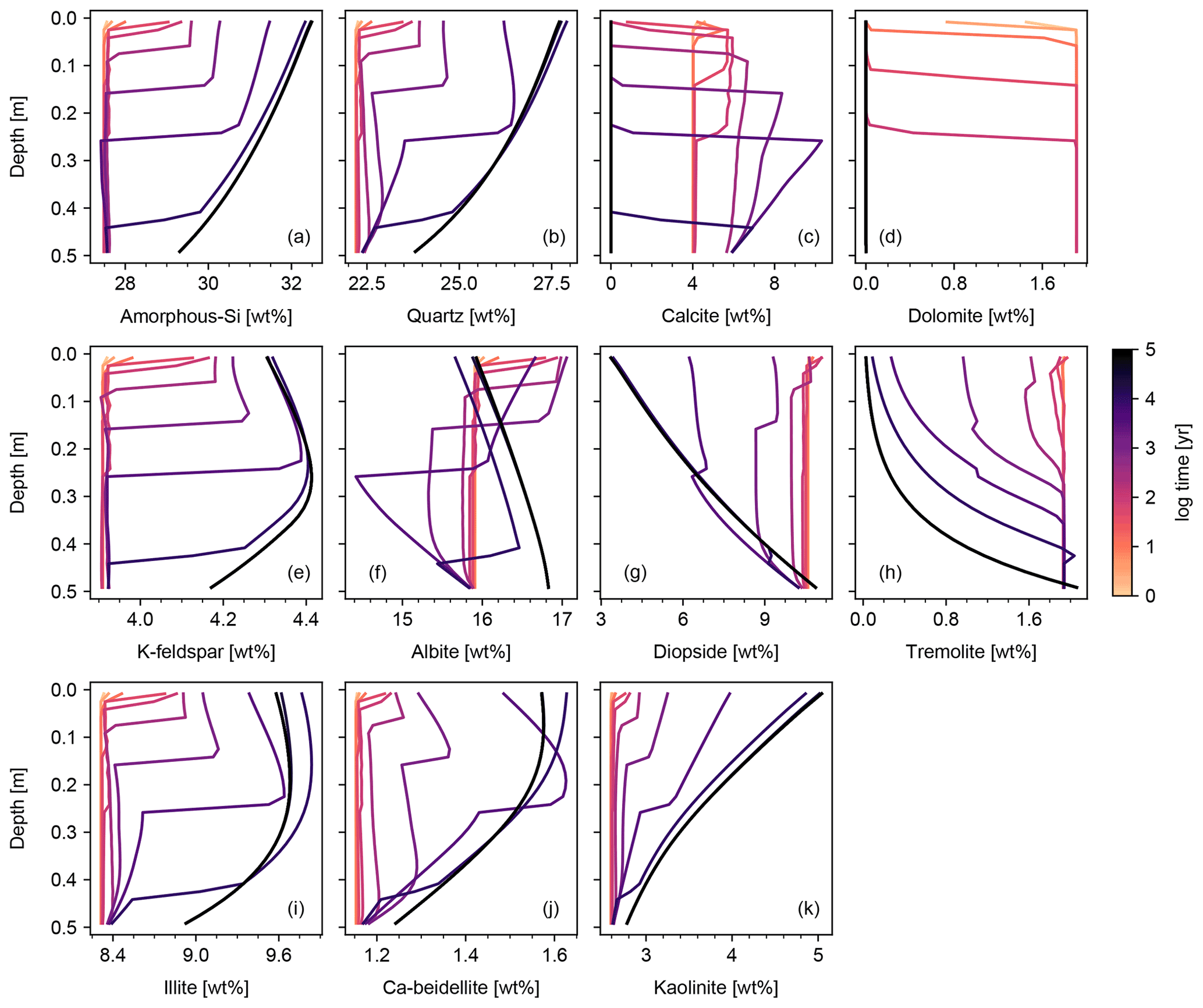
Figure 3Soil concentrations of solid species in simulation of abiotic weathering at Site 1 in Table 8. See Table 7 for the details on the boundary conditions of the simulation.
In the default version of SCEPTER in which PSDs are not tracked, surface area is calculated by combining Eqs. (27)–(30), (40) and (41). When PSD tracking is enabled in the surface area calculation, the governing equation for PSD (Eq. 31) is discretized by a finite-difference method and solved time-implicitly as for the solution of the governing equation for solid species (Eq. 1). The PSD shifts caused by net volume change by dissolution/precipitation (the second term on the right-hand side of Eq. 31) are enforced from solutions of Eqs. (32), (34) and (35) by the first-order upwind finite-difference scheme and the Newton–Raphson method. A PSD for parent rock is imposed as the lower boundary condition. This procedure is repeated for individual solid species when calculating species-specific PSDs and surface areas ((4) in Sect. 2.2.6). By default, SCEPTER considers the PSD calculation converged when the difference in particle number from the previous iteration is less than 10−12 times the maximum number of particles. The calculated PSD is truncated below one particle per cubic meter of bulk soil for a given radius bin.
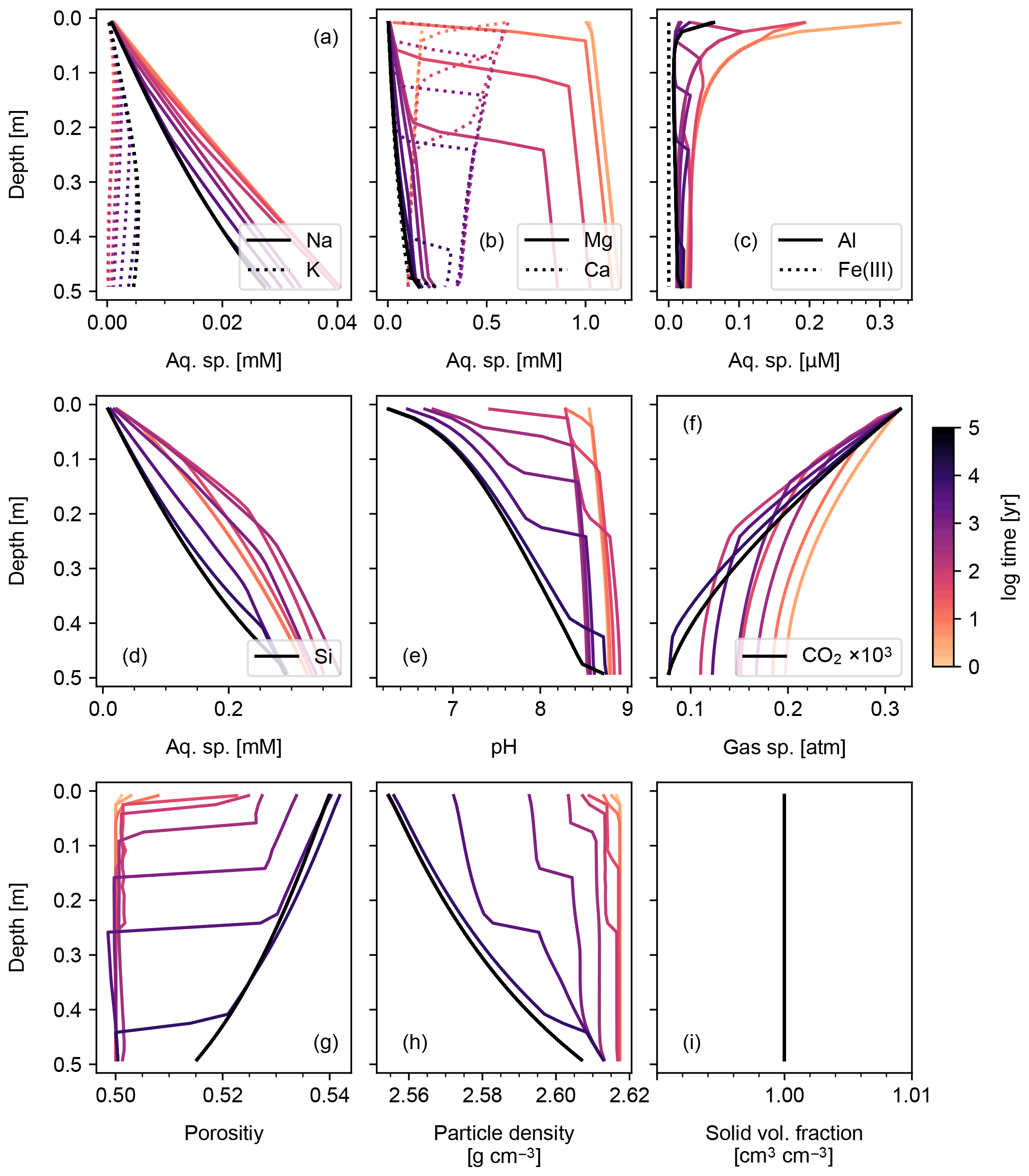
Figure 4Simulation of abiotic weathering at Site 1 in Table 8. Porewater concentrations of aqueous species and pH are plotted in (a)–(d) and (e), respectively; concentrations of soil gases in (f); soil porosity and particle density in (f) and (g), respectively; ratio of the total volume of solid species against solid space specified with porosity in (h). See Table 7 for details on the boundary conditions of the simulation.
2.4 User input
2.4.1 Independent variables
Solid, aqueous and gas species to be tracked in a simulation are listed in individual input files (slds.in, solutes.in and gases.in). If a user wants
to include reactions other than dissolution/precipitation reactions
specified for individual solid species, the ID string of the extra reaction
(e.g., fe2o2 in Table 6 for aqueous Fe(II) oxidation by O2) can be
specified in another input file (exrxns.in).
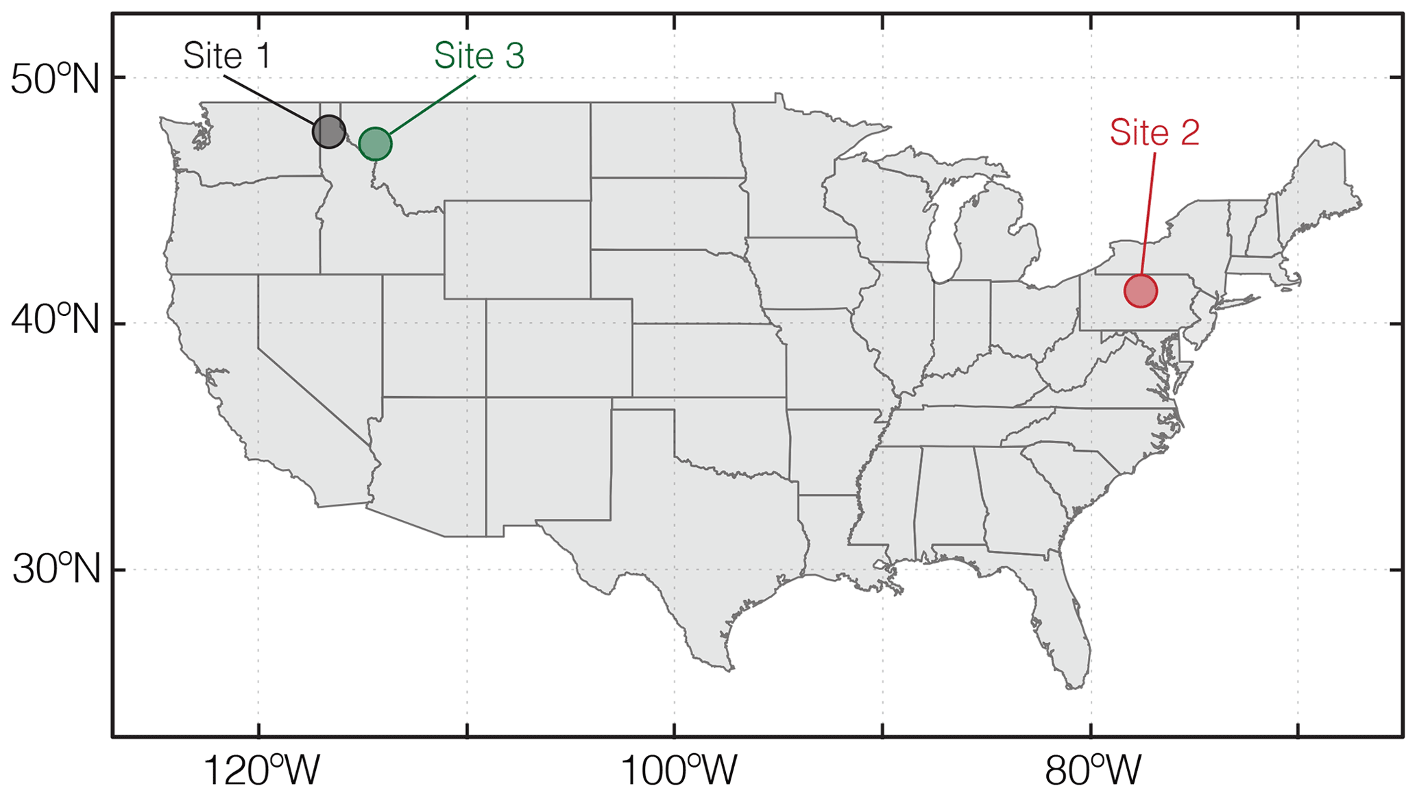
Figure 5Locations of natural weathering sites whose boundary conditions are tabulated in Table 8 and utilized for example simulations in Sect. 3.
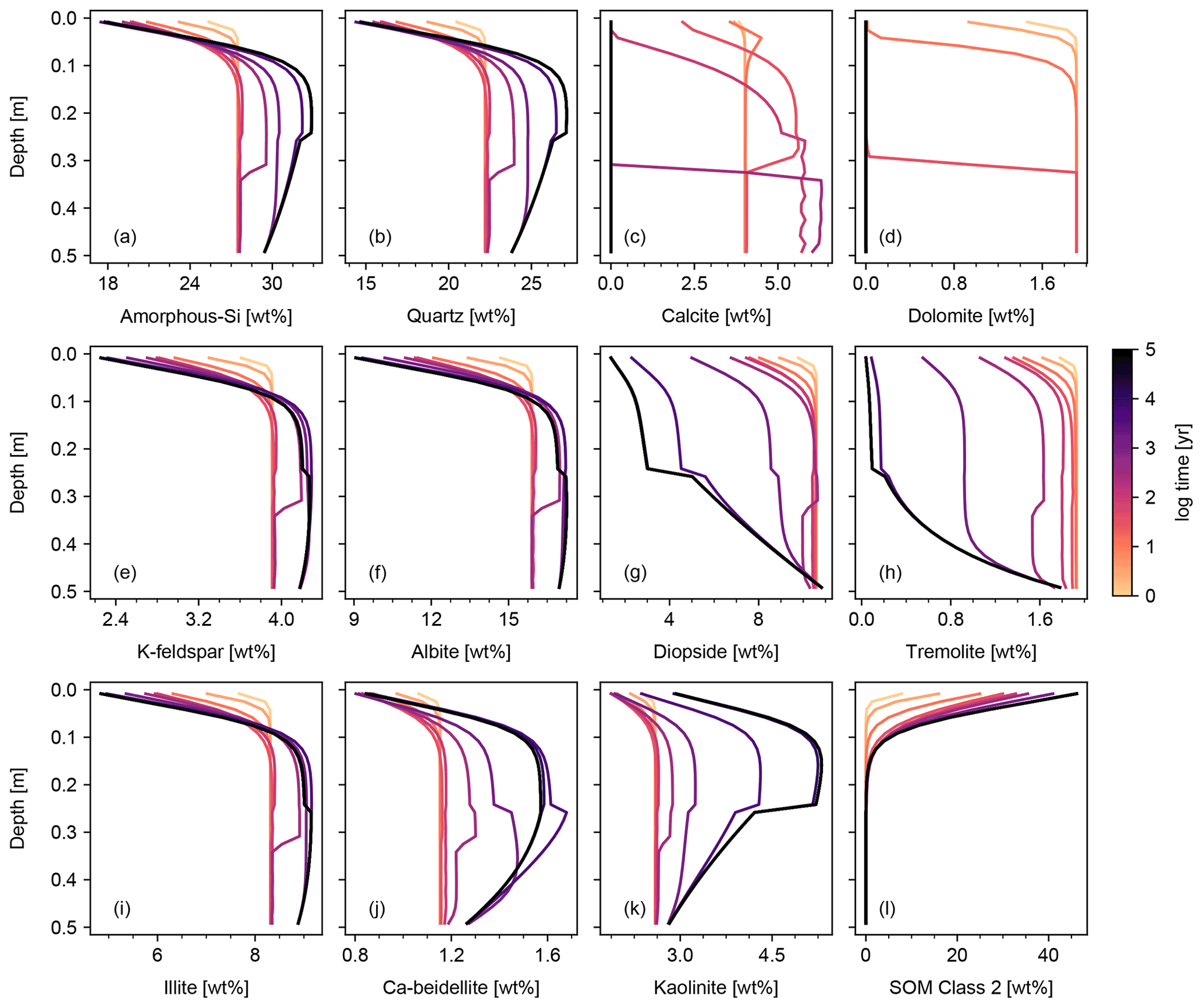
Figure 6Simulation of biotic weathering at Site 1 in Table 8. Shown are concentrations of simulated solid species. Note that the model configuration is the same as that for Fig. 3 except that soil respiration and bio-mixing are included.
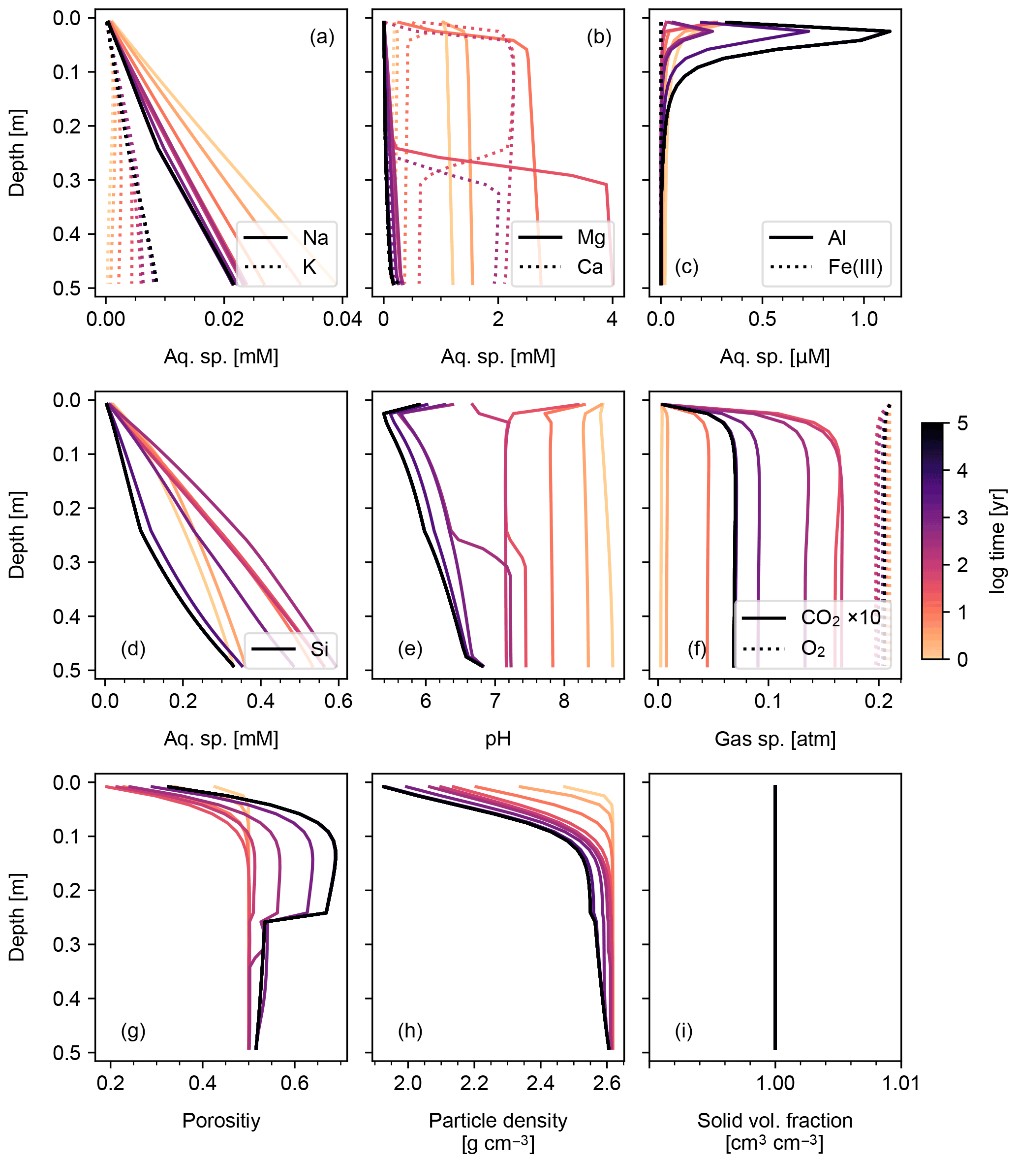
Figure 7Simulation of biotic weathering at Site 1 in Table 8. Panels show the depth profiles of aqueous and gas species and soil physical properties as in Fig. 4 except that simulation includes soil respiration and bio-mixing.
2.4.2 Boundary conditions
Fundamental variables such as grid size, total depth of simulated soil,
water flux, water table depth, surface water saturation, mixing layer
thickness, application rate of powdered rock feedstock, OM rain flux,
temperature, initial/bottom uplift rate and initial soil porosity are specified in the input file frame.in. Modifying options for, e.g., mixing regime and method of surface area calculation can be made by modifying
another input file, switches.in. One can also specify whether to do a
re-start experiment in switches.in, and, when doing a re-start experiment, the previous experiment from which the current simulation should be restarted
can be specified in frame.in.
Surface area of parent rock is calculated from the average effective radius
of particles specified in frame.in. When one chooses to calculate specific
surface areas for individual solid species, different average radius values
can be assigned to different solid species in the input file sa.in. The particle size distributions for parent rock are calculated assuming log-normal distributions with 1 SD centered at the radius value(s) input
from frame.in or sa.in. Currently, the PSD for OM rain is assumed to be the
same as that for parent rock, while the PSD for rock feedstock needs to be
specified within the source codes by providing mean radius(es) and standard
deviation(s).
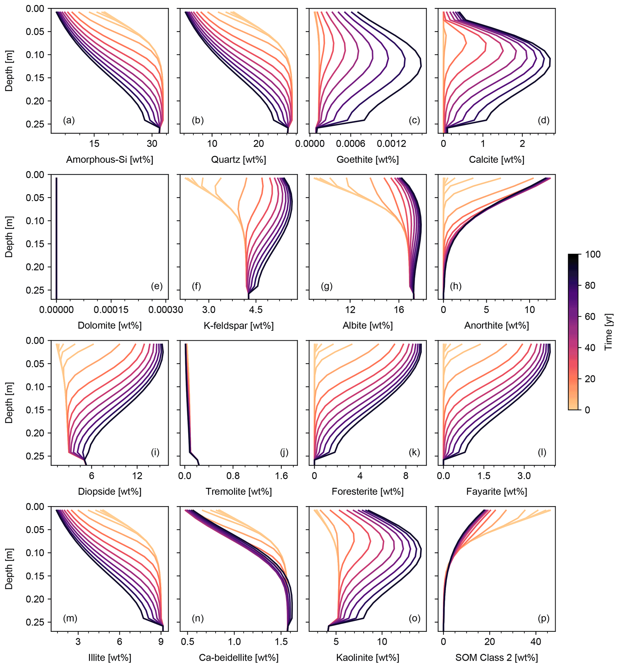
Figure 8Basalt powder application at Site 1 in Table 8. Panels show the depth profiles of simulated solid species as in Fig. 6, except that basalt powder is continuously added at a rate of 40 t ha−1 yr−1 and plots are focused on the soil mixed layer (0–25 cm).
Boundary conditions for solid, aqueous and gas species need to be provided as parent rock, rainwater and atmospheric concentrations, respectively, in
the corresponding input files (parentrock.in, rain.in and atm.in).
Compositions of solids being introduced at the soil surface must also be
specified using individual input files (dust.in and OM_rain.in, respectively). In the case of time-varying changes to water flux,
temperature and water saturation ratio, a series of additional input files is necessary (T_temp.in, q_temp.in and
Wet_temp.in). See the full README information included in the code repository for further details (code availability).

Figure 9Basalt powder application at Site 1 in Table 8. Panels show the depth profiles of aqueous and gas species and soil physical properties as in Fig. 7 except that basalt powder is continuously added at a rate of 40 t ha−1 yr−1.
2.4.3 Initial conditions
At the beginning of a simulation, concentrations of solid, aqueous and gas species are assumed to be the same as those of parent rock, rainwater and atmosphere, respectively, which can be specified by the user with the corresponding input files (see above). Initial surface areas as well as PSDs at all depths are assumed to be the same as those of parent rock specified by the user. Porosity similarly takes the initial value provided by the user at all depths. When the volume sum of all chosen solid species in the parent rock is less than the solid fraction implied by the initial/bottom porosity, then an imaginary “bulk” species is additionally tracked to occupy the void space whose physical properties are assumed to be the same as those of kaolinite but with no reactions allowed (Rθ≡0 with θ= “bulk”). When the volume sum of all chosen solid species exceeds the assigned value from the initial/bottom porosity, the parent rock concentrations of chosen solid species are rescaled to be consistent with the initial/bottom porosity. Volume conservation (Eq. 16) is thus always satisfied by SCEPTER (cf. Archer et al., 2002; Munhoven, 2021; Kanzaki et al., 2021).
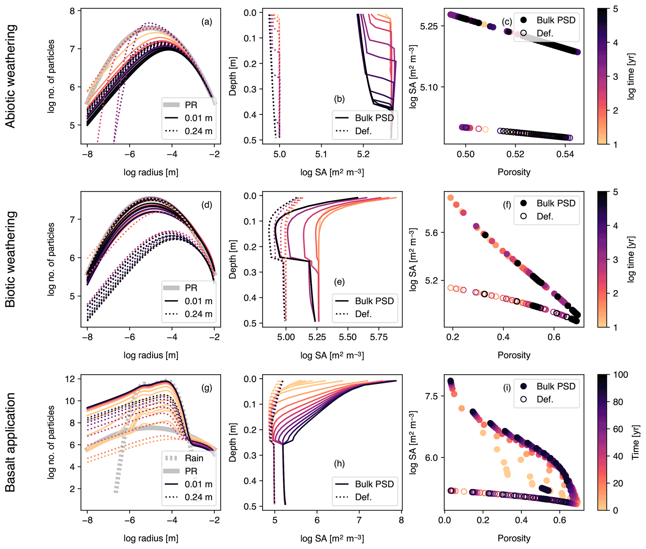
Figure 10Simulations of abiotic weathering (a–c), biotic weathering (d–f) and basalt powder application (g–i) at Site 1 in Table 8 with surface area calculated based on tracked particle size distribution (PSD) for bulk soil. PSDs at surface and bottom of soil mixed layer are shown in (a), (d) and (g). Pore surface area per unit pore volume is plotted against depth (b, e, h) or porosity (c, f, i) and compared with the calculation with the default surface area parameterization. See Sect. 3.1.4 and Table 7 for the details on the boundary conditions of the simulations.
To illustrate the features and capabilities of SCEPTER, we present a series of idealized example experiments. First, the basic features of SCEPTER are illustrated by simulating abiotic weathering (e.g., without SOM and mixing; Sect. 3.1.1), biotic weathering (with SOM and mixing; Sect. 3.1.2), and basalt application (with SOM, mixing, and additional mineral supplied at the soil surface; Sect. 3.1.3) scenarios with the default surface area calculation method. The same set of simulations is then repeated using the PSD-based surface area calculation (Sect. 3.1.4). Finally, we show a series of SCEPTER runs driven by observational data from a subset of relatively pristine natural systems coupled with the USGS soil chemistry database (U.S. Geological Survey, 2016), and track time-dependent CO2 capture across a range of timescales (Sect. 3.2).
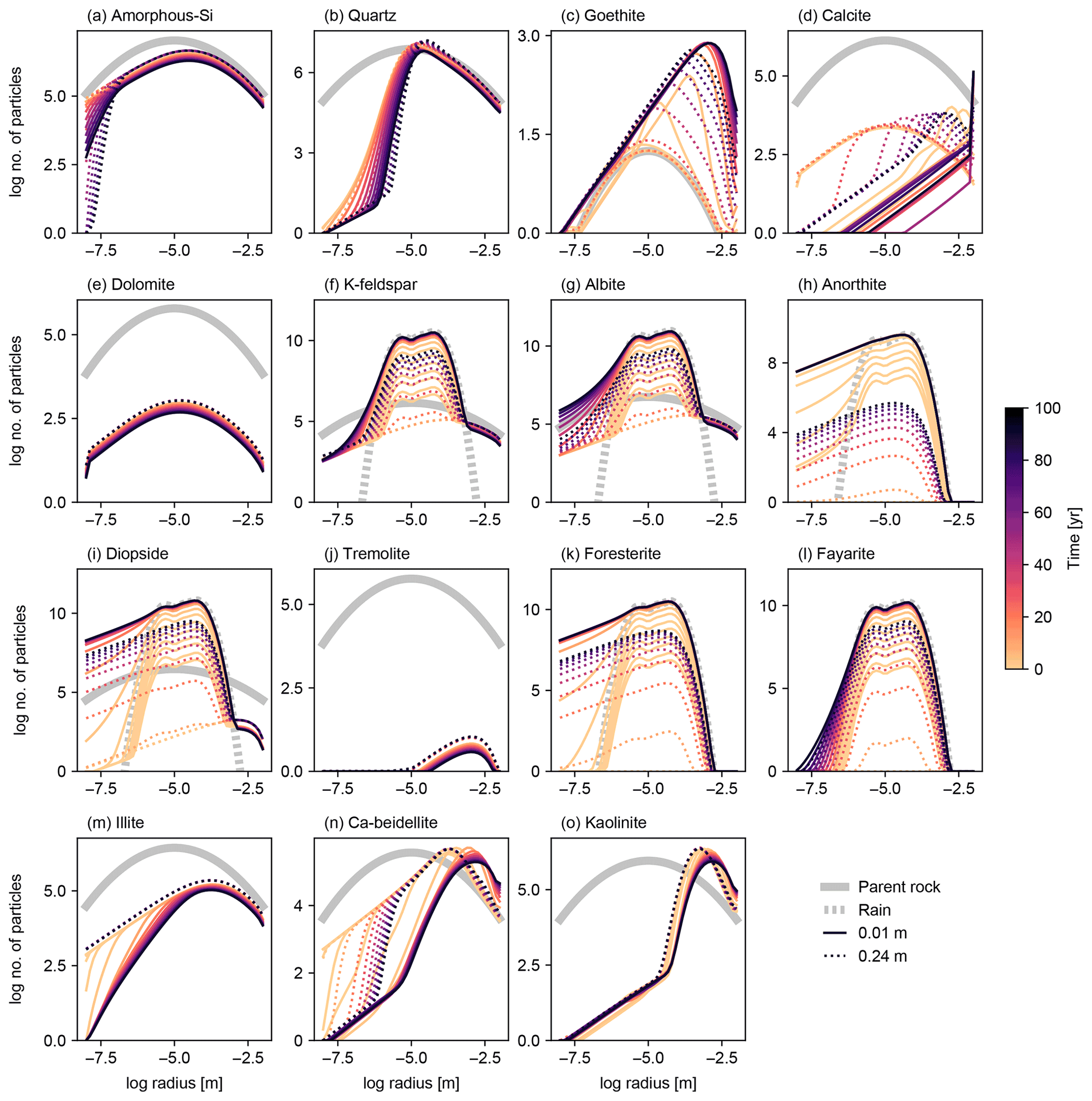
Figure 11Particle size distributions (PSDs) at surface and bottom of soil mixed layer for individual solid species in simulation of basalt powder application at Site 1 in Table 8 with the surface area calculated based on tracked PSDs for individual solid species. See Sect. 3.1.4 and Table 7 for the details on the boundary conditions of the simulation.
3.1 Illustration of basic features of SCEPTER
3.1.1 Abiotic weathering
The simplest configuration of SCEPTER explored here is the simulation of abiotic weathering of albite and pyrite, respectively (Figs. 1, 2; Table 7). Dominant controls on and locations of reaction fronts of albite and pyrite are consistent with simpler models (e.g., water flow for albite weathering, and water table depth on pyrite weathering; e.g., Kanzaki et al., 2020). SCEPTER allows tracking of time-dependent changes to gradients in solid and solute species, which in the simple abiotic cases evolve as expected – in the first case, with gradual conversion of albite to kaolinite and progressive release of Si and Na to soil pore fluids (Fig. 1), and in the second case a sharp reaction front along which pyrite is converted to goethite and O2 is drown down to negligible levels at the water table depth (Fig. 2). Overall depth-dependent changes to porosity and particle density are relatively small in both of these simplified abiotic cases (Figs. 1 and 2). Note that, in these examples input parent-rock concentrations of minerals (10 wt % albite and 0.56 wt % pyrite) are smaller than inferred from assumed initial/bottom porosity (0.1). Thus, an imaginary bulk species is simulated along with the above minerals (not shown in Figs. 1 and 2), ensuring that volume conservation is satisfied (Eq. 16).

Figure 12Surface area of individual solid species per unit pore volume plotted against depth (focused on mixed layer; 0–25 cm) in simulation of basalt powder application at Site 1 in Table 8 with the surface area calculated based on tracked PSDs for individual solid species (“Full PSD”). The pore surface areas per unit pore volume calculated with the default parameterization (“Def.”) and based on PSD for bulk soil (“Bulk PSD”) are also plotted for comparison. See Sect. 3.1.4 and Table 7 for details on the boundary conditions of the simulation.
Results of a more complicated abiotic weathering simulation are shown in Figs. 3 and 4, in which SCEPTER is fed by the bulk mineralogy and climatological boundary conditions for a natural weathering site (Site 1 in Fig. 5 and Table 8) (see also Sect. 3.2). Here, we assume zero OM rain to the system and no mixing to exclude biotic aspects of weathering (cf. Sect. 3.1.2) and run an abiotic weathering simulation to reach a steady state. Because production of soil CO2 is minimized without a flux of OM to the soil surface, soil CO2 drops at depth as a result of cation release (and alkalinity production) from mineral dissolution. Primary silicates such as albite and diopside are largely dissolved. Initially, carbonate phases dissolve at the surface but precipitate at depth. However, as the system approaches steady state (∼104 years), carbonate phases redissolve and secondary clays accumulate (Fig. 3). Solute profiles evolve in accordance with mineral profiles, and once again overall changes to soil porosity and particle density are relatively small (Fig. 4). In this case, SCEPTER does not include the imaginary bulk species (Fig. 3; Tables 7 and 8), but volume conservation is nevertheless always satisfied.
3.1.2 Biotic weathering: addition of organic matter flux to soil surface and soil mixing
Following the expansion of vascular plant ecosystems across Earth's land surface, natural weathering generally occurs in the presence of SOM and soil respiration (cf. Volk, 1987; Berner, 1992; Kanzaki and Kump, 2017; Ibarra et al., 2019; Wen et al., 2021). Indeed, the recycling of SOM represents a critical component of soil acid–base chemistry and CO2 cycling and is likely to change significantly across a range of ecosystems in the coming century (e.g., Brovkin et al., 2013; McGuire et al., 2018). The current version of SCEPTER can simulate up to three classes of SOM of varying lability. By default, the lability of each class of SOM progressively decreases, with turnover times of 1, 8 and 103 years, respectively. However, the intrinsic SOM labilities can be scaled arbitrarily for a range of applications (e.g., manure application, biochar amendment, etc.), provided that reliable kinetic data are implemented. The OM flux to the soil surface can either be specified arbitrarily or can be scaled to above-ground net primary production; by default, SCEPTER scales the OM flux to the soil surface as 1.5 times above ground primary production, following Beerling et al. (2020). Note that additional biotic factors relating to the soil OM cycling, such as secretion of organic acids and uptake of nutrients and/or cations by plants, are not treated in the current version of the model but will be included in a future release.
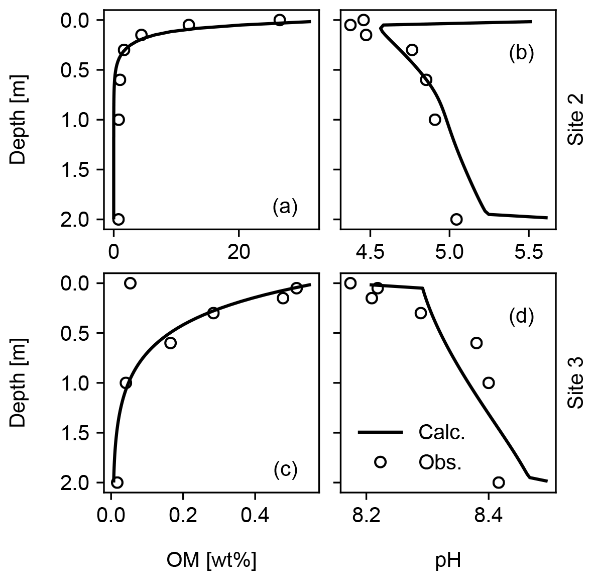
Figure 13Model fit to observed depth profiles of soil OM and pH for Sites 2 and 3 in Table 8. See Sect. 3.2.1 for the details.
Figures 6 and 7 show results of a simple biotic weathering experiment in which Class 2 SOM (here taken to represent a generalized “natural” SOM; e.g., Chen et al., 2010) and soil bioturbation (here termed Fickian mixing) are added to the experimental conditions for the abiotic weathering experiment shown in Figs. 3 and 4. As a result of SOM respiration, soil CO2 builds up as high as >0.01 atm as weathering proceeds (Fig. 7). This buildup in CO2 significantly lowers soil pH, which promotes dissolution of primary mineral phases and leads to an increase in porosity around the mid-depth of the soil mixed layer (∼0.1 m). A range of silicate mineral phases becomes unstable and dissolves with the presence of SOM respiration (e.g., compare Figs. 3 and 6). On a timescale of ∼102 years, carbonate phases dissolve at the surface of the model domain and precipitate at the bottom of the soil column, but all carbonate phases ultimately dissolve at steady state.
At steady state, soil CO2 is around 0.006 atm, still more than 10 times higher than the ambient atmospheric level. SOM dominates amongst the solid phases near the soil surface, below which clays and Si-oxide phases become more dominant (Fig. 6). Dissolved cations are concentrated only at the deepest depths of the model domain, consistent with the observed distributions of mineral phases (Fig. 7). Dissolved Al shows higher concentrations in the biotic weathering scenario relative to the abiotic weathering regime due to increased solubility at lower pH (e.g., compare Figs. 4 and 7). Average grains (aggregates) of soil become less dense closer to the surface because they consist more of SOM whose particle density is relatively small (1.5 g cm−3) compared with those of other solid phases (Fig. 7). Note that volume conservation is again satisfied throughout the experiment even with a continuous flux of OM to the soil surface (Fig. 7i).
3.1.3 Basalt powder application: enhanced rock weathering (ERW)
A useful user option for simulating enhanced rock weathering in SCEPTER is the ability to conduct a re-start experiment from the previously conducted simulation. This feature allows the user to first run a spinup experiment – for instance, to fit the model to current observations at a given location – and then examine the impacts of adding crushed rock feedstock in a transient experiment branched from the spinup simulation. Here, we illustrate this procedure by conducting a re-start experiment including basalt powder application to the soil surface branched from the biotic weathering experiment for Site 1 (Table 8 and Fig. 5) presented in Sect. 3.1.2, which has been spun up to steady state by running the model for ∼105 years.
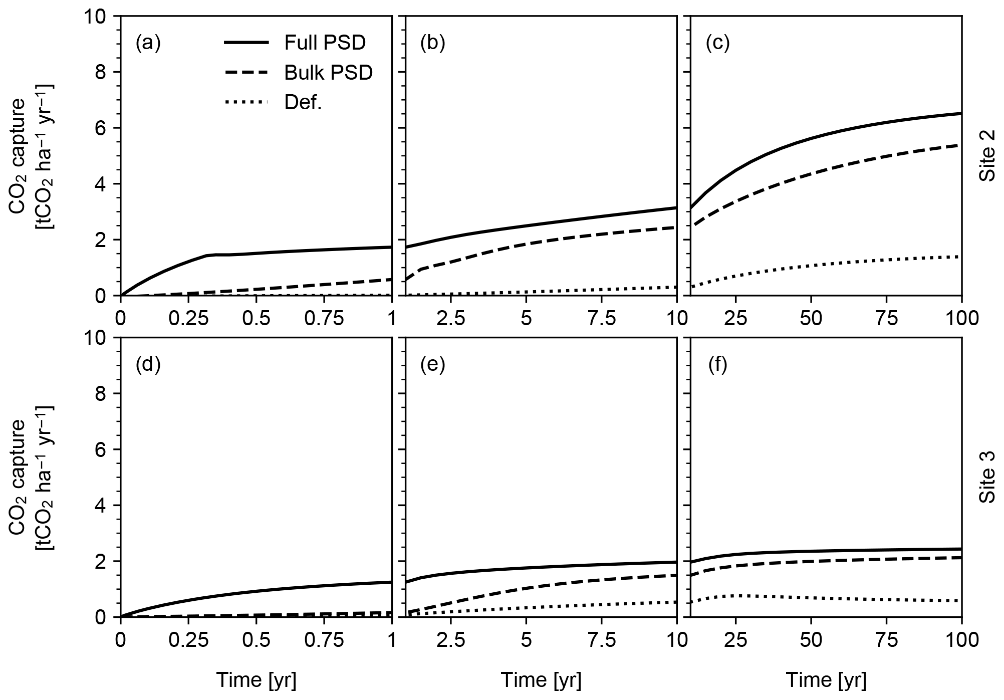
Figure 14CO2 capture predicted in simulations of continuous basalt powder application at Sites 2 and 3 in Table 8 with the surface area calculation based on the assumed hydraulic radius (“Def.”), tracked PSD for bulk soil (“Bulk PSD”) and tracked PSDs for individual solid species (“Full PSD”). See Sect. 3.2.2 for details.
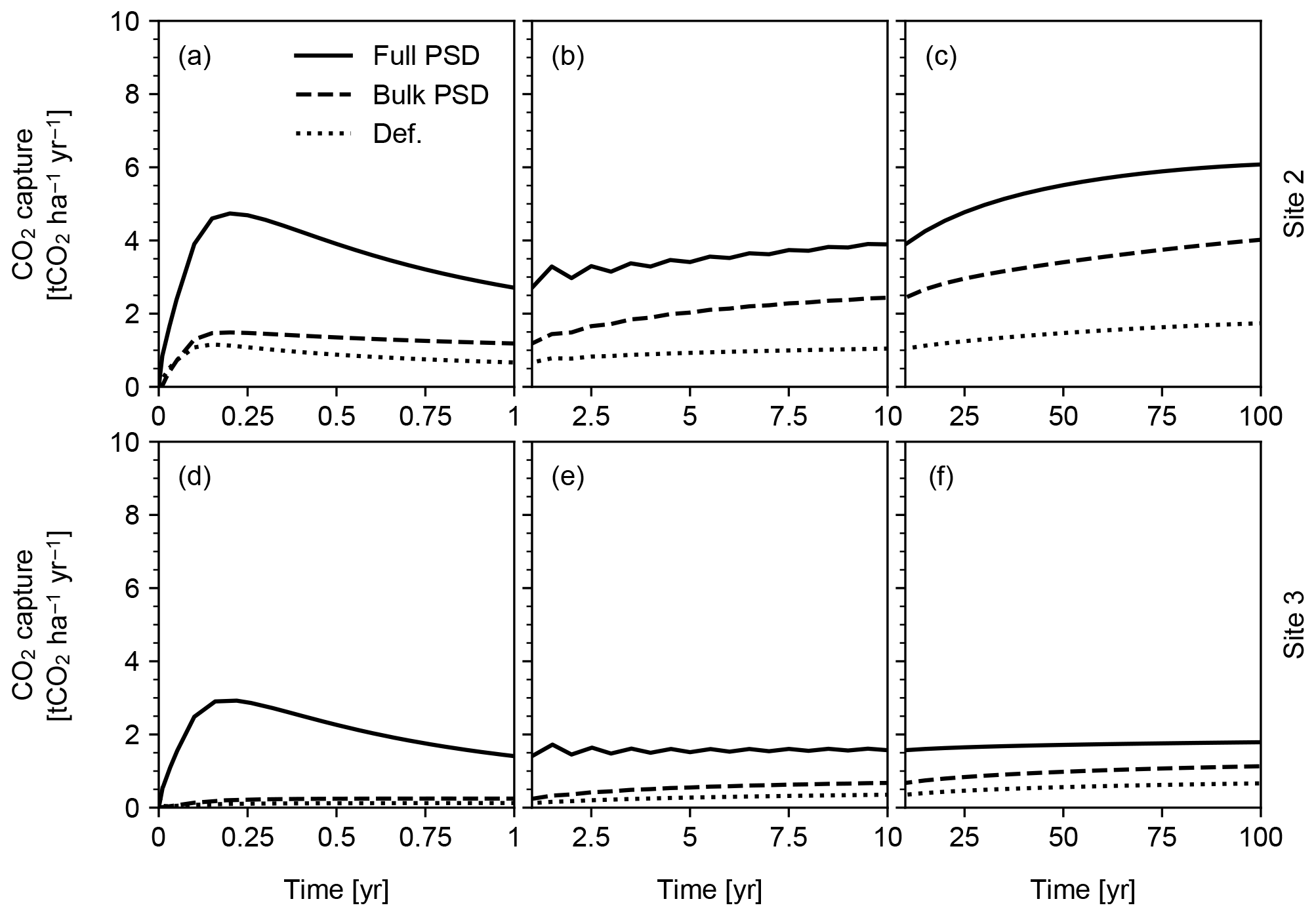
Figure 15CO2 capture predicted in simulations of pulsative basalt application at Sites 2 and 3 in Table 8. Milled basalt (dominated by 5, 20, 50 and 70 µm particles) is applied non-continuously and homogeneously mixed at the soil surface. See Sect. 3.2.2 for details.
We set the application rate of basalt powder at 40 t ha−1 yr−1, whose mineral composition is assumed to be the same as that adopted for basalt by Beerling et al. (2020). Because basalt powder will generally contain significant amounts of reduced Fe, we implement aqueous Fe(II) oxidation by O2 as an extra reaction in the re-start experiment (Table 7). Application of basalt powder adds a large amount of primary minerals to surface soils, where they have generally been depleted during spinup to steady state (Fig. 8). One outcome of this is that carbonate phases precipitate during basalt application (Fig. 8d) together with kaolinite and goethite and later with smectite (Fig. 8c, n and o). There is a drop in SOM near the soil surface (Fig. 8p), despite the OM rain flux remaining identical to that in the spinup simulation (Sect. 3.1.2). Rained minerals with high solubility and reactivity result in similar depth profiles to that of SOM (e.g., Fig. 8h, k, l and p), while those with lower solubility/reactivity tend to accumulate at depth (e.g., Fig. 8f and g). Soil CO2 accumulates as high as >0.075 atm because surface porosity drops significantly following basalt application (Fig. 9g). Soil O2 becomes depleted over time, in part due to the porosity change, but also because of the introduction of Fe(II) oxidation as an additional O2 sink that does not exist during the spinup simulation. Once again, volume conservation is satisfied even with a significant external flux of mineral phases to the system (Fig. 9i).
3.1.4 The impact of particle size tracking
In order to illustrate the potential use of optional PSD tracking for calculating the mineral surface area in SCEPTER, we repeated the same experiments presented above for Site 1 (Fig. 5 and Table 8; Sects. 3.1.1–3.1.3) while implementing mineral surface area based on tracked PSDs for bulk soil minerals, including a dynamic roughness factor (see (2)–(4) in Sect. 2.2.6). For parent rock, we assume a log-normal size distribution centered at 10 µm with a standard deviation of 1 log unit (i.e., fPR(r)∝ exp(−(log r+ 5)2/2), where fPR is defined as the PSD of parent rock and r is the particle radius in meters). We assign the same distribution to the OM rain flux in the biotic weathering experiment, while basalt powder is assumed to have a PSD that mixes equally four log-normal distributions centered at 5, 20, 50 and 70 µm with standard deviations of 0.2 log units. Note that because our intention is to illustrate the basic behavior of the model, the PSD parameterizations adopted here are not necessarily realistic for a given application (cf. Eberl et al., 1998; Sklar et al., 2017; Beerling et al., 2020) and should be modified within the code by the user when necessary.
Concentration profiles for solid, aqueous, and gas species are largely similar to those obtained with the default surface area scheme, particularly for the abiotic and biotic natural weathering experiments, because the resultant surface areas are fairly similar (Fig. 10b, c, e and f). In the abiotic weathering experiment, particles with small radii dissolve and disappear rapidly, particularly at shallower depths (Fig. 10a). In the biotic weathering experiment, the soil surface receives an OM rain flux whose particle distribution is assumed to be the same as that of parent rock, and thus the relative depletion of small particles in the PSD is most prominent near the bottom of the mixed layer (dotted curves in Fig. 10d), where mineral dissolution is significant but the particle input from the OM rain flux is attenuated.
In contrast, mineral surface area in the basalt application case is significantly different between the default and PSD-tracking schemes (Fig. 10h and i). This is because the crushed rock particles, whose size distributions are centered at 5–70 µm with relatively small standard deviations, become the dominant constituent of the surface mixed layer of soil (e.g., solid and dotted curves in Fig. 10g). The dominance of particles with a relatively small radius results in a large surface area per unit mass, leading to a large surface area difference between the PSD-based and default methods (Fig. 10h and i).
To further explore the impact of PSD tracking on mineral surface area, we conducted another set of experiments identical to those above but with PSD tracking for individual solid species (rather than the bulk solid phase). We present the results of a basalt application experiment in which PSD tracking has the most prominent effects on the surface area calculation (Figs. 11 and 12) and compare these with the default surface area parameterization and the calculation based on the PSD for bulk soil. Individually tracked PSDs are different between solid species (Fig. 11) and also differ from the PSD for bulk soil (Fig. 10g). For example, solid species that are introduced to the system only through basalt powder application show patterns similar to the PSD specified for basalt powder, with smaller particles being produced via dissolution as time proceeds (e.g., Fig. 11k), and those precipitated as a result of basalt powder application show significant particle growth (Fig. 11c, d, n and o). Accordingly, surface area depth profiles vary between solid species and are significantly different from those simulated with the default method and the PSD tracked only for bulk soil (Fig. 12). In the basalt application scenario, surface areas for individual solid species increase more significantly when tracking species-specific PSDs relative to those calculated based on PSD for bulk soil (e.g., Fig. 12k). On the other hand, surface areas of solid species that are not supplied through basalt application are generally smaller when tracking species-specific PSDs than tracking only PSD for bulk soil (e.g., Fig. 12j and m). Note that surface areas of secondary minerals (e.g., Fig. 12d) are not significantly reduced compared with those of dissolving primary minerals that are not supplied through basalt application (Fig. 12j) because surface roughness is accounted for. Overall, when conducting experiments involving addition of particles whose size distributions are significantly different from the PSD of the parent rock, we recommend PSD tracking for individual solid species though computationally more demanding.
3.2 Example ERW application – time-dependent CO2 capture following basalt addition at contrasting pristine hinterland sites
As a final illustration of model capability, we estimate time-dependent CO2 capture during continuous and pulsed basalt application at two pristine hinterland watersheds in the US. The two watersheds are obtained by delineating all watersheds corresponding to the USGS river gauges (U.S. Geological Survey, 2016) using GRASS GIS (GRASS Development Team, 2017), followed by selecting watersheds that have experienced minimum human interferences (watersheds that have a population density of less than one person per square kilometer; land proportion of cultivated vegetation less than 1 %; land proportion of urban land less than 1 %). The mineral compositions for these two pristine watersheds are derived from the USGS soil chemistry database (U.S. Geological Survey, 2016). We emphasize that the sites used for illustration are not optimized for CO2 capture, given that they are characterized by relatively low runoff and temperature (Table 8). The only aim here is to demonstrate the ability of SCEPTER to examine first-order controls on CO2 capture during enhanced rock weathering, and these sites, given the lack of human intervention, have a more predictable history than sites that have been strongly directly influenced by human activity. Experimental conditions are the same as those adopted in Sect. 3.1.3 and 3.1.4 except for the used sites (Sites 2 and 3; Table 8 and Fig. 5).
3.2.1 Tuned spinup to observational data
When detailed observational data are available for a specific individual site of potential enhanced rock weathering, one can perform site-specific tuning at spinup prior to crushed rock application. As an illustration, we tune SCEPTER to observed OM and pH profiles at two pristine hinterland sites (Sites 2 and 3 in Table 8; see Fig. 5 for their locations) assuming Fickian mixing (e.g., bioturbation) (Fig. 13). For Site 2, optimized OM and pH profiles can be obtained by introducing an additional class of SOM (e.g., Class 3 SOM introduced at 0.1016 times the Class 2 SOM rain flux) and assuming slightly different labilities for the two classes of SOM relative to the default values (5 and 85 years for turnover of SOM Classes 2 and 3, respectively). In tuning to Site 3, no extra SOM class is added, but the rain flux and turnover time are modified for Class 2 SOM to 0.64 g C m−2 yr−1 and 1600 years, respectively. The simulated soil thickness and mixed layer depth are extended to 2 m to fit to the observed OM and pH profiles, and the total grid number is doubled (60). Surface area is calculated during spinup with the default method assuming 100 and 7 µm of average particle radii for Sites 2 and 3, respectively. The remaining boundary conditions are defined in the same way as detailed in the biotic weathering experiment for Site 1 (Table 7; Sect. 3.1.2) but using the parameter values specified for Sites 2 and 3 in Table 8.
Observed soil OM and pH depth profiles are reproduced well by SCEPTER with minimal tuning (Fig. 13). Fickian mixing is effective only where solid concentrations are relatively high and is thus particularly intense close to the surface. Therefore, Fickian mixing introduces some difficulty in reproducing the SOM profile for Site 2 at depth (∼1 wt %, Table 9). In contrast, because a relatively low SOM reactivity is assumed, Fickian mixing closely reproduces SOM concentrations throughout the soil column for Site 3, except for the low surface value. In any case, this exercise demonstrates that SCEPTER can be readily tuned using site-specific observations in order to optimize ERW capture for local boundary conditions and that in general minimal effort should be required to perform robust site-specific tuning across a very wide range of soil pore fluid pH and organic matter content (Fig. 13).
3.2.2 Time-dependent variation in CO2 capture
We perform two sets of time-dependent CO2 capture experiments, applying crushed basalt at a rate of 40 ton ha−1 yr−1 to the tuned spinups discussed in Sect. 3.2.1. In the first set, basalt is applied continuously throughout the simulation, and Fickian mixing is applied across all solid phases. In the second set, we perform pulsed basalt addition in which crushed basalt is applied at the same overall annual application rate and homogeneously mixed into the soil, but only during the initial part of each year (0.1 year), while mixing occurs in the Fickian regime throughout the remainder of the year. We perform all simulations across the range of PSD options in SCEPTER (see above), including the default setting, bulk PSD tracking and full PSD tracking.
We find that the surface area scheme significantly impacts predicted CO2 capture (Fig. 14). In particular, significant differences between the default parameterization and PSD-based methods (Fig. 14) suggest that explicit differentiation of particle sizes between added powder and existent soil/rock is crucial for accurate predictive quantification of carbon capture during enhanced rock weathering. The results also suggest that species-specific PSD tracking is fundamental particularly for the prediction of short-term CO2 capture efficiency (<10 years; Fig. 14a and d). It is also clear that the CO2 capture rate depends strongly on the chosen site and associated background boundary conditions (compare Fig. 14a–c with d–f; see also Tables 8 and 9), particularly over longer time horizons.
Pulsed basalt addition leads to a significant short-term enhancement in CO2 capture, but on century timescales overall capture rates for both sites are comparable regardless of whether feedstock amendment is continuous or pulsed (Figs. 14 and 15). The long-term CO2 capture rates estimated here are broadly comparable with previous estimates (e.g., Beerling et al., 2020), but our model predicts significant induction time before achieving maximum CO2 capture at a given feedstock application rate (e.g., 0.16 capture efficiency (≡ mass ratio of captured CO2 against deployed basalt) in 100 years at Site 2 vs. 0.15–0.25 capture efficiency in 10 years by Beerling et al., 2020). However, we emphasize that these simulations are only meant to be illustrative of the capabilities of the model and that the sites and ERW deployment procedure have not been optimized for maximizing CO2 capture rates. As a result, these results should not in any way be interpreted as conclusive or generalizable with respect to CO2 capture rate, efficiency and induction time. In addition, the potential difference in induction time for CDR should be evaluated in a more comprehensive intercomparison study in which model parameterizations, boundary conditions and experimental setups are aligned as much as possible. The purpose here is simply to illustrate the differences between parameterizations of particle size and surface area.
SCEPTER is a traceable code with the capability to comprehensively realize phenomena occurring within soil weathering systems, including abiotic/biotic weathering of minerals, mixing of soil particles and addition of OM/minerals under natural or managed conditions. The model is equipped with options to calculate surface areas of soil particles by tracking particle size distributions through time and space. This specific feature may be of particular importance for calculating the cost performance of terrestrial enhanced rock weathering, as a significant component of both economic cost and secondary CO2 emissions is the grinding and transport of rock feedstocks (e.g., Renforth, 2012). Application of the model to US soil data indicates that it is well suited to capturing the major mineral transformations and solute fluxes attendant to natural weathering.
The current version of the model can serve several purposes relevant for natural weathering, carbon cycle dynamics and managed soil chemistry. Ongoing model developments include a full mechanistic implementation and validation of nutrient (P, N, and K) cycles and nutrient uptake and secretion of organic acids by plants (e.g., Lawrence et al., 2014; Perez-Fodich and Derry, 2019), inclusion of size-dependent changes in the particle solubility and nucleation kinetic barrier when tracking species-specific PSDs (e.g., Hochella, 2003; Perez et al., 2008; Emmanuel and Ague, 2011), implementation of a wider range of potential management practices and coupling to Earth system model frameworks in order to more fully explore the dynamics of CDR (e.g., Ridgwell et al., 2007; Holden et al., 2016; Taylor et al., 2016). We suggest that SCEPTER can be a powerful tool for predicting and diagnosing the effects of enhanced rock weathering on existing soil systems, particularly following robust site-specific tuning against background observations.
The source codes of the model are available at GitHub (https://github.com/lithos-erw/SCEPTER, last access: 24 February 2022). The specific version of the model used in this paper is tagged as “v0.9” and has been assigned a doi (https://doi.org/10.5281/zenodo.5835413, Kanzaki, 2022). A readme file on the web provides the instructions for executing the simulations.
YK and CTR designed and implemented the model with significant contributions from the other authors. SZ compiled and filtered observational data. All the authors contributed to the experimental design, and YK conducted the experiments and analyzed the results. All the authors contributed to the writing of the paper.
The contact author has declared that neither they nor their co-authors have any competing interests.
Publisher's note: Copernicus Publications remains neutral with regard to jurisdictional claims in published maps and institutional affiliations.
We are grateful to two anonymous reviewers for their useful comments and to Andrea Stenke for editorial handling.
This paper was edited by Andrea Stenke and reviewed by two anonymous referees.
Aachib, M., Mbonimpa, M., and Aubertin, M.: Measurement and prediction of the oxygen diffusion coefficient in unsaturated media, with applications to soil covers, Water Air Soil Pollut., 156, 163–193, https://doi.org/10.1023/B:WATE.0000036803.84061.e5, 2004.
Archer, D. E., Morford, J. L., and Emerson, S. R.: A model of suboxic sedimentary diagenesis suitable for automatic tuning and gridded global domains, Global Biogeochem. Cy., 16, 1017, https://doi.org/10.1029/2000GB001288, 2002.
Astete, C. E., Thibodeaux, L. J., and Constant, W. D.: Semi-volatile organic compounds as chemical tracers for estimating soil particle biodiffusion coefficients: application of polychlorinated biphenyls in earthworm bioturbation at a grassland site, Soil Sci., 181, 457–464, https://doi.org/10.1097/SS.0000000000000178, 2016.
Beaulieu, E., Goddéris, Y., Donnadieu, Y., Labat, D., and Roelandt, C.: High sensitivity of the continental-weathering carbon dioxide sink to future climate change, Nat. Clim. Change, 2, 346–349, https://doi.org/10.1038/nclimate1419, 2012.
Beerling, D. J., Kantzas, E. P., Lomas, M. R., Wade, P., Eufrasio, R. M., Renforth, P., Sarkar, B., Andrews, M. G., James, R. H., Pearce, C. R., Mercure, J.-F., Pollitt, H., Holden, P. B., Edwards, N. R., Khanna, M., Koh, L., Quegan, S., Pidgeon, N. F., Janssens, I. A., Hansen, J., and Banwart, S. A.: Potential for large-scale CO2 removal via enhanced rock weathering with croplands, Nature, 583, 242–248, https://doi.org/10.1038/s41586-020-2448-9, 2020.
Berner, R. A.: Weathering, plants, and the long-term carbon cycle, Geochim. Cosmochim. Ac., 56, 3225–3231, https://doi.org/10.1016/0016-7037(92)90300-8, 1992.
Bibi, I., Singh, B., and Silvester, E.: Dissolution of illite in saline–acidic solutions at 25 ∘ C, Geochim. Cosmochim. Ac., 75, 3237–3249, https://doi.org/10.1016/j.gca.2011.03.022, 2011.
Bolton, E. W., Berner, R. A., and Petsch, S. T.: The weathering of sedimentary organic matter as a control on atmospheric O2: II. Theoretical modeling, Am. J. Sci., 306, 575–615, https://doi.org/10.2475/08.2006.01, 2006.
Boudreau, B. P.: Diagenetic Models and Their Implication, Springer, ISBN 978-3-642-64399-6, 1997.
Boudreau, B. P., Choi, J., Meysman, F., and François-Carcaillet, F.: Diffusion in a lattice-automaton model of bioturbation by small deposit feeders, J. Mar. Res., 59, 749–768, https://doi.org/10.1357/002224001762674926, 2001.
Brantley, S. L. and Lebedeva, M.: Learning to read the chemistry of regolith to understand the Critical Zone, Annu. Rev. Earth Planet. Sci., 39, 387–416, https://doi.org/10.1146/annurev-earth-040809-152321, 2011.
Brantley, S. L. and Mellott, N. P.: Surface area and porosity of primary silicate minerals, Am. Mineral., 85, 1767–1783, https://doi.org/10.2138/am-2000-11-1220, 2000.
Brantley, S. L., Kubicki, J. D., and White, A. F.: Kinetics of Water-Rock Interaction, Springer, ISBN 978-0-387-73562-7, 2008.
Brovkin, V., Boysen, L., Arora, V. K., Boisier, J. P., Cadule, P., Chini, L., Claussen, M., Friedlingstein, P., Gayler, V., van den Hurk, B. J. J. M., Hurtt, G. C., Jones, C. D., Kato, E., de Noblet-Ducoudré, N., Pacifico, F., Pongratz, J., and Weiss, M.: Effect of anthropogenic land-use and land-cover changes on climate and land carbon storage in CMIP5 projections for the twenty-first century, J. Climate, 26, 6859–6881, https://doi.org/10.1175/JCLI-D-12-00623.1, 2013.
Chen, S., Huang, Y., Zou, J., Shen, Q., Hu, Z., Qin, Y., Chen, H., and Pan, G.: Modeling interannual variability of global soil respiration from climate and soil properties, Agr. Forest Meteorol., 150, 590–605, https://doi.org/10.1016/j.agrformet.2010.02.004, 2010.
Chen, Z., Guo, M., and Wang, W.: Variations in soil erosion resistance of gully head along a 25-year revegetation age on the Loess Plateau, Water, 12, 3301, https://doi.org/10.3390/w12123301, 2020.
Choi, J., Francois-Carcaillet, F., and Boudreau, B. P.: Lattice-automaton bioturbation simulator (LABS): implementation for small deposit feeders, Comput. Geosci., 28, 213–222, https://doi.org/10.1016/S0098-3004(01)00064-4, 2002.
Clennell, M. B.: Tortuosity: a guide through the maze, in: Developments in Petrophysics, edited by: Lovell, M. A. and Harvey, P. K., Geological Society Special Publication No. 122, 299–344, https://doi.org/10.1144/GSL.SP.1997.122.01.18, 1997.
Delany, J. M. and Lundeen, S. R.: The LLNL thermochemical database, Lawrence Livermore National Laboratory Report UCRL-21658, Lawrence Livermore National Laboratory, 1990.
Eberl, D. D., Drits, V. A., and Środoń, J.: Deducing growth mechanisms for minerals from the shapes of crystal size distributions, Am. J. Sci., 298, 499–533, https://doi.org/10.2475/ajs.298.6.499, 1998.
Elberling, B. and Nicholson, R. V.: Field determination of sulphide oxidation rates in mine tailings, Water Resour. Res., 32, 1773–1784, https://doi.org/10.1029/96WR00487, 1996.
Emmanuel, S. and Ague, J. J.: Impact of nano-size weathering products on the dissolution rates of primary minerals, Chem. Geol., 282, 11–18, https://doi.org/10.1016/j.chemgeo.2011.01.002, 2011.
Emmanuel, S. and Berkowitz, B.: Mixing-induced precipitation and porosity evolution in porous media, Adv. Water Resour., 28, 337–344, https://doi.org/10.1016/j.advwatres.2004.11.010, 2005.
Fanchi, J. R.: Principles of Applied Reservoir Simulation, 4th Edn., Elsevier, ISBN 978-0-12-815563-9, 2018.
Fekete, B. M., Vörösmarty, C. J., and Grabs, W.: High-resolution fields of global runoff combining observed river discharge and simulated water balances, Global Biogeochem. Cy., 16, 15-1–15-10, https://doi.org/10.1029/1999GB001254, 2002.
Fick, S. E. and Hijmans, R. J.: WorldClim 2: new 1-km spatial resolution climate surfaces for global land areas, Int. J. Climatol., 37, 4302–4315, https://doi.org/10.1002/joc.5086, 2017.
Fuss, S., Ganadell, J. G., Peters, G. P., Tavoni, M., Andrew, R. M., Ciais, P., Jackson, R. B., Jones, C. D., Kraxner, F., Nakicenovic, N., Le Quéré, C., Raupach, M. R., Sharifi, A., Smith, P., and Yamagata, Y.: Betting on negative emissions, Nat. Clim. Change, 4, 850–853, https://doi.org/10.1038/nclimate2392, 2014.
Gasser, T., Cuivarch, C., Tachiiri, K., Jones, C. D., and Ciais, P.: Negative emissions physically needed to keep global warming below 2 ∘ C, Nat. Commun., 6, 7958, https://doi.org/10.1038/ncomms8958, 2015.
Gíslason, S. R. and Arnósson, S.: Dissolution of primary basaltic minerals in natural waters: saturation state and kinetics, Chem. Geol., 105, 117–135, https://doi.org/10.1016/0009-2541(93)90122-Y, 1993.
Goldberg, E. D. and Koide, M.: Geochronological studies of deep sea sediments by the ionium/thorium method, Geochim. Cosmochim. Ac., 26, 417–450, https://doi.org/10.1016/0016-7037(62)90112-6, 1962.
Goll, D. S., Ciais, P., Amann, T., Buermann, W., Chang, J., Eker, S., Hartmann, J., Janssens, I., Li, W., Obersteiner, M., Penuelas, J., Tanaka, K., and Vicca, S: Potential CO2 removal from enhanced weathering by ecosystem responses to powdered rock, Nat. Geosci, 14, 545–549, https://doi.org/10.1038/s41561-021-00798-x, 2021.
Goddéris, Y., François, L. M., Probst, A., Schott, J., Moncoulon, D., Labat, D., and Viville, D.: Modelling weathering processes at the catchment scale: The WITCH numerical model, Geochim. Cosmochim. Ac., 70, 1128–1147, https://doi.org/10.1016/j.gca.2005.11.018, 2006.
Goddéris, Y., Brantley, S. L., François, L. M., Schott, J., Pollard, D., Déqué, M., and Dury, M.: Rates of consumption of atmospheric CO2 through the weathering of loess during the next 100 yr of climate change, Biogeosciences, 10, 135–148, https://doi.org/10.5194/bg-10-135-2013, 2013.
GRASS Development Team: Geographic Resources Analysis Support System (GRASS GIS) Software, Version 7.2, Open Source Geospatial Foundation, http://grass.osgeo.org (last access: 20 April 2022), 2017.
Hartmann, J., West, A. J., Renforth, P., Köhler, P., De La Rocha, C. L., Wolf-Gladrow, D. A., Dürr, H. H., and Scheffran, J.: Enhanced chemical weathering as a geoengineering strategy to reduce atmospheric carbon dioxide, supply nutrients, and mitigate ocean acidification, Rev. Geophys., 51, 113–149, https://doi.org/10.1002/rog.20004, 2013.
Hengl, T., Mendes de Jesus, J., Heuvelink, G. B. M., Gonzalez, M. R., Kilibarda, M., Blagotić, A., Shangguan, W., Wright, M. N., Geng, X., Bauer-Marschallinger, B., Guevara, M. A., Vargas, R., MacMillan, R. A., Batjes, N. H., Leenaars, J. G. B., Ribeiro, E., Wheeler, I., Mantel, S., and Kempen, B.: SoilGrids250m: Global gridded soil information based on machine learning, PloS One 12, e0169748, https://doi.org/10.1371/journal.pone.0169748, 2017.
Hochella Jr., M. F.: Nanoscience and technology: the next revolution in the Earth sciences, Earth Planet. Sc. Lett., 203, 593–605, https://doi.org/10.1016/S0012-821X(02)00818-X, 2003.
Holden, P. B., Edwards, N. R., Fraedrich, K., Kirk, E., Lunkeit, F., and Zhu, X.: PLASIM–GENIE v1.0: a new intermediate complexity AOGCM, Geosci. Model Dev., 9, 3347–3361, https://doi.org/10.5194/gmd-9-3347-2016, 2016.
Ibarra, D. E., Caves Rugenstein, J. K., Bachan, A., Baresch, A., Lau, K. V., Thomas, D. L., Lee, J.-E., Boyce, C. K., and Chamberlain, C. P.: Modeling the consequences of land plant evolution on silicate weathering, Am. J. Sci., 319, 1–43, https://doi.org/10.2475/01.2019.01, 2019.
Iggland, M. and Mazzotti, M.: Population balance modeling with size-dependent solubility: Ostwald ripening, Cryst. Growth Des., 12, 1489–1500, https://doi.org/10.1021/cg201571n, 2012.
IPCC: 2006 IPCC Guidelines for National Greenhouse Gas Inventories, IPCC, ISBN 4-88788-032-4, 2006.
IPCC: Global Warming of 1.5∘ C, IPCC, https://doi.org/10.1017/9781009157940, 2018.
Jarvis, N. J., Taylor, A., Larsbo, M., Etana, A., and Rosén, K.: Modelling the effects of bioturbation on the re-distribution of 137Cs in an undisturbed grassland soil, Eur. J. Soil Sci., 61, 24–34, https://doi.org/10.1111/j.1365-2389.2009.01209.x, 2010.
Jia, M., Jacques, D., Gérard, F., Su, D., Mayer, K. U., and Šimůnek, J.: A benchmark for soil organic matter degradation under variably saturated flow conditions, Comput. Geosci., 25, 1359–1377, https://doi.org/10.1007/s10596-019-09862-3, 2021.
Kanzaki, Y.: lithos-erw/SCEPTER: submission to GMDD (v0.9), Zenodo [code], https://doi.org/10.5281/zenodo.5835413, 2022.
Kanzaki, Y. and Kump, L. R.: Biotic effects on oxygen consumption during weathering: Implications for the second rise of oxygen, Geology, 45, 611–614, https://doi.org/10.1130/G38869.1, 2017.
Kanzaki, Y. and Murakami, T.: Estimates of atmospheric CO2 in the Neoarchean–Paleoproterozoic from paleosols, Geochim. Cosmochim. Ac., 159, 190–219, https://doi.org/10.1016/j.gca.2015.03.011, 2015.
Kanzaki, Y. and Murakami, T.: Estimates of atmospheric O2 in the Paleoproterozoic from paleosols, Geochim. Cosmochim. Ac., 174, 263–290, https://doi.org/10.1016/j.gca.2015.11.022, 2016.
Kanzaki, Y. and Murakami, T.: Effects of atmospheric composition on apparent activation energy of silicate weathering: I. Model formulation, Geochim. Cosmochim. Ac., 223, 159–186, https://doi.org/10.1016/j.gca.2017.10.008, 2018.
Kanzaki, Y., Boudreau, B. P., Kirtland Turner, S., and Ridgwell, A.: A lattice-automaton bioturbation simulator with coupled physics, chemistry, and biology in marine sediments (eLABS v0.2), Geosci. Model Dev., 12, 4469–4496, https://doi.org/10.5194/gmd-12-4469-2019, 2019.
Kanzaki, Y., Brantley, S. L., and Kump, L. R.: A numerical examination of the effect of sulfide dissolution on silicate weathering, Earth Planet. Sc. Lett., 539, 116239, https://doi.org/10.1016/j.epsl.2020.116239, 2020.
Kanzaki, Y., Hülse, D., Kirtland Turner, S., and Ridgwell, A.: A model for marine sedimentary carbonate diagenesis and paleoclimate proxy signal tracking: IMP v1.0, Geosci. Model Dev., 14, 5999–6023, https://doi.org/10.5194/gmd-14-5999-2021, 2021.
Köhler, P., Hartmann, J., and Wolf-Gladrow, D. A.: Geoengineering potential of artificially enhanced silicate weathering of olivine, P. Natl. Acad. Sci. USA, 107, 20228–20233, https://doi.org/10.1073/pnas.1000545107, 2010.
Köhler, P., Abrams, J. F., Völker, C., Hauck, J., and Wolf-Gladrow, D. A.: Geoengineering impact of open ocean dissolution of olivine on atmospheric CO2, surface ocean pH and marine biology, Environ. Res. Lett., 21, 014009, https://doi.org/10.1088/1748-9326/8/1/014009, 2013.
Larsen, I. J., Montgomery, D. R., and Greenberg, H. M.: The contribution of mountains to global denudation, Geology, 42, 527–530, https://doi.org/10.1130/G35136.1, 2014.
Lawrence, C., Harden, J., and Maher, K.: Modeling the influence of organic acids on soil weathering, Geochim. Cosmochim. Ac., 139, 487–507, https://doi.org/10.1016/j.gca.2014.05.003, 2014.
LeBlanc, S. E. and Fogler, H. S.: Population balance modeling of the dissolution of polydisperse solids: rate limiting regimes, AIChE J., 33, 54–63, https://doi.org/10.1002/aic.690330108, 1987.
Le Quéré, C., Andrew, R. M., Friedlingstein, P., Sitch, S., Hauck, J., Pongratz, J., Pickers, P. A., Korsbakken, J. I., Peters, G. P., Canadell, J. G., Arneth, A., Arora, V. K., Barbero, L., Bastos, A., Bopp, L., Chevallier, F., Chini, L. P., Ciais, P., Doney, S. C., Gkritzalis, T., Goll, D. S., Harris, I., Haverd, V., Hoffman, F. M., Hoppema, M., Houghton, R. A., Hurtt, G., Ilyina, T., Jain, A. K., Johannessen, T., Jones, C. D., Kato, E., Keeling, R. F., Goldewijk, K. K., Landschützer, P., Lefèvre, N., Lienert, S., Liu, Z., Lombardozzi, D., Metzl, N., Munro, D. R., Nabel, J. E. M. S., Nakaoka, S., Neill, C., Olsen, A., Ono, T., Patra, P., Peregon, A., Peters, W., Peylin, P., Pfeil, B., Pierrot, D., Poulter, B., Rehder, G., Resplandy, L., Robertson, E., Rocher, M., Rödenbeck, C., Schuster, U., Schwinger, J., Séférian, R., Skjelvan, I., Steinhoff, T., Sutton, A., Tans, P. P., Tian, H., Tilbrook, B., Tubiello, F. N., van der Laan-Luijkx, I. T., van der Werf, G. R., Viovy, N., Walker, A. P., Wiltshire, A. J., Wright, R., Zaehle, S., and Zheng, B.: Global Carbon Budget 2018, Earth Syst. Sci. Data, 10, 2141–2194, https://doi.org/10.5194/essd-10-2141-2018, 2018.
Li, D. D., Jacobson, A. D., and McInerney, D. J.: A reactive-transport model for examining tectonic and climatic controls on chemical weathering and atmospheric CO2 consumption in granitic regolith, Chem. Geol., 365, 300–42, https://doi.org/10.1016/j.chemgeo.2013.11.028, 2014.
Li, Y.-H. and Gregory, S.: Diffusion of ions in sea water and in deep-sea sediments, Geochim. Cosmochim. Ac., 38, 703–714, https://doi.org/10.1016/0016-7037(74)90145-8, 1974.
Liddicoat, S. K., Wiltshire, A. J., Jones, C. D., Arora, V. K., Brovkin, V., Cadule, P., Hajima, T., Lawrence, D. M., Pongratz, J., Schwinger, J., Séférian, R., Tjiputra, J. F., and Ziehn, T.: Compatible fossil fuel CO2 emissions in the CMIP6 Earth system models' historical and Shared Socioeconomic Pathway experiments of the twenty-first century, J. Climate, 34, 2853–2875, https://doi.org/10.1175/JCLI-D-19-0991.1, 2021.
Maggi, F., Gu, C., Riley, W. J., Hornberger, G. M., Venterea, R. T., Xu, T., Spycher, N., Steefel, C., Miller, N. L., and Oldenburg, C. M.: A mechanistic treatment of the dominant soil nitrogen cycling processes: Model development, testing, and application, J. Geophys. Res., 113, G02016, https://doi.org/10.1029/2007JG000578, 2008.
Maher, K., Steefel, C. I., White, A. F., and Stonestrom, D. A.: The role of reaction affinity and secondary minerals in regulating chemical weathering rates at the Santa Cruz Soil Chronosequence, California, Geochim. Cosmochim. Ac., 73, 2804–2831, https://doi.org/10.1016/j.gca.2009.01.030, 2009.
Massmann, W. J.: A review of the molecular diffusivities of H2O, CO2, CH4, CO, O3, SO2, NH3, N2O, NO, and NO2 in air, O2 and N2 near STP, Atmos. Environ., 32, 1111–1127, https://doi.org/10.1016/S1352-2310(97)00391-9, 1998.
Mayer, L. M., Schick, L. L., Hardy, K. R., Wagai, R., and McCarthy, J.: Organic matter in small mesopores in sediments and soils, Geochim. Cosmochim. Ac., 68, 3863–3872, https://doi.org/10.1016/j.gca.2004.03.019, 2004.
McGuire, A. D., Lawrence, D. M., Koven, C., Clein, J. S., Burke, E., Chen, G., Jafarov, E., MacDougall, A. H., Marchenko, S., Nicolsky, D., Peng, S., Rinke, A., Ciais, P., Gouttevin, I., Hayes, D. J., Ji, D., Krinner, G., Moore, J. C., Romanovsky, V., Schädel, C., Schaefer, K., Schuur, E. A. G., and Zhuang, Q.: Dependence of the evolution of carbon dynamics in the northern permafrost region on the trajectory of climate change, P. Natl. Acad. Sci. USA, 115, 3882–3887, https://doi.org/10.1073/pnas.1719903115, 2018.
McKibben, M. A. and Barnes, H. L.: Oxidation of pyrite in low temperature acidic solutions: Rate laws and surface textures, Geochim. Cosmochim. Ac., 50, 1509–1520, https://doi.org/10.1016/0016-7037(86)90325-X, 1986.
Minx, J. C., Lamb, W. F., Callaghan, M. W., Fuss, S., Hilaire, J., Creutzig, F., Amann, T., Beringer, T., de Oliveria Garcia, W., Hartmann, J., Khanna, T., Lenzi, D., Luderer, G., Nemet, G. F., Rogelj, J., Smith, P., Luis Vincente Vincente, J., Wilcox, J., and del Mar Zamora Dominguez, M.: Negative emissions–Part 1: Research landscape and synthesis, Environ. Res. Lett., 13, 063001, https://doi.org/10.1088/1748-9326/aabf9b, 2018.
Moore, J., Lichtner, P. C., White, A. F., and Brantley, S. L.: Using a reactive transport model to elucidate differences between laboratory and field dissolution rates in regolith, Geochim. Cosmochim. Ac., 93, 235–261, https://doi.org/10.1016/j.gca.2012.03.021, 2012.
Munhoven, G.: Model of Early Diagenesis in the Upper Sediment with Adaptable complexity – MEDUSA (v. 2): a time-dependent biogeochemical sediment module for Earth system models, process analysis and teaching, Geosci. Model Dev., 14, 3603–3631, https://doi.org/10.5194/gmd-14-3603-2021, 2021.
Navarre-Sitchler, A. and Brantley, S.: Basalt weathering across scales, Earth Planet. Sc. Lett., 261, 321–334, https://doi.org/10.1016/j.epsl.2007.07.010, 2007.
Nicholson, R. V., Gillham, R. W., and Reardon, E. J.: Pyrite oxidation in carbonate-buffered solution: 2. Rate control by oxide coatings, Geochim. Cosmochim. Ac., 54, 395–402, https://doi.org/10.1016/0016-7037(90)90328-I, 1990.
Palandri, J. L. and Kharaka, Y. K.: A Compilation of Rate Parameters of Water-Mineral Interaction Kinetics for Application to Geochemical Modeling, Geological Survey, Menlo Park CA, 2004.
Parkhurst, D. L. and Appelo, C. A. J.: Description of input and examples for PHREEQC version 3: a computer program for speciation, batch-reaction, one-dimensional transport, and inverse geochemical calculations, US Geological Survey, https://doi.org/10.3133/tm6A43, 2013.
Perez-Fodich, A. and Derry, L. A.: Organic acids and high soil CO2 drive intense chemical weathering of Hawaiian basalts: Insights from reactive transport models, Geochim. Cosmochim. Ac., 349, 173–198, https://doi.org/10.1016/j.gca.2019.01.027, 2019.
Perez, M., Dumont, M., and Acevedo-Reyes, D.: Implementation of classical nucleation and growth theories for precipitation, Acta Mater., 56, 2119–2132, https://doi.org/10.1016/j.actamat.2007.12.050, 2008.
Pritchard, D. T. and Currie, J. A.: Diffusion of coefficients of carbon dioxide, nitrous oxide, ethylene and ethane in air and their measurement, J. Soil Sci., 33, 175–184, https://doi.org/10.1111/j.1365-2389.1982.tb01757.x, 1982.
Ragnarsdóttir, K. V.: Dissolution kinetics of heulandite at pH 2–12 and 25 ∘ C, Geochim. Cosmochim. Ac., 57, 2439–2449, https://doi.org/10.1016/0016-7037(93)90408-O, 1993.
Rau, G. H., Knauss, K. G., Langer, W. H., and Caldeira, K.: Reducing energy-related CO2 emissions using accelerated weathering of limestone, Energy, 32, 1471–1477, https://doi.org/10.1016/j.energy.2006.10.011, 2007.
Rebreanu, L., Vanderborght, J. P., and Chou, L.: The diffusion coefficient of dissolved silica revisited, Mar. Chem., 112, 230–233, https://doi.org/10.1016/j.marchem.2008.08.004, 2008.
Renforth, P.: The potential of enhanced weathering in the UK, Int. J. Greenh. Gas Control., 10, 229–243, https://doi.org/10.1016/j.ijggc.2012.06.011, 2012.
Renforth, P. and Henderson, G.: Assessing ocean alkalinity for carbon sequestration, Rev. Geophys., 55, 636–674, https://doi.org/10.1002/2016RG000533, 2017.
Renforth, P., Pogge von Strandmann, P. A. E, and Henderson, G. M.: The dissolution of olivine added to soil: Implications for enhanced weathering, Appl. Geochem., 61, 109–118, https://doi.org/10.1016/j.apgeochem.2015.05.016, 2015.
Ridgwell, A., Hargreaves, J. C., Edwards, N. R., Annan, J. D., Lenton, T. M., Marsh, R., Yool, A., and Watson, A.: Marine geochemical data assimilation in an efficient Earth System Model of global biogeochemical cycling, Biogeosciences, 4, 87–104, https://doi.org/10.5194/bg-4-87-2007, 2007.
Robie, R. A. Hemingway, B. S., and Fisher, J. R.: Thermodynamic properties of minerals and related substances at 298.15 K and 1 bar (105 pascals) pressure and at higher temperatures, US Geological Survey, 1978.
Rogelj, J., Shindell, D., Jiang, K., Fifita, S., Forster, P., Ginzburg, V., Handa, C., Kobayashi, S., Kriegler, E., Mundaca, L., Séférian, R., Vilariño, M. V., Calvin, K., Emmerling, J., Fuss, S., Gillett, N., He, C., Hertwich, E., Höglund-Isaksson, L., Huppmann, D., Luderer, G., McCollum, D.L., Meinshausen, M., Millar, R., Popp, A., Purohit, P., Riahi, K., Ribes, A., Saunders, H., Schädel, C., Smith, P., Trutnevyte, E., Xiu, Y., Zhou, W., Zickfeld, K., Flato, G., Fuglestvedt, J., Mrabet, R., and Schaeffer, R.: Mitigation pathways compatible with 1.5∘ C in the context of sustainable development, IPCC, https://doi.org/10.1017/9781009157940.004, 2018.
Roland, M., Serrano-Ortiz, P., Kowalski, A. S., Goddéris, Y., Sánchez-Cañete, E. P., Ciais, P., Domingo, F., Cuezva, S., Sanchez-Moral, S., Longdoz, B., Yakir, D., Van Grieken, R., Schott, J., Candell, C., and Janssens, I. A.: Atmospheric turbulence triggers pronounced diel pattern in karst carbonate geochemistry, Biogeosciences, 10, 5009–5017, https://doi.org/10.5194/bg-10-5009-2013, 2013.
Safari, V., Arzpeyma, G., Raschchi, F., and Mostoufi, N.: A shrinking particle–shrinking core model for leaching of a zinc ore containing silica, Int. J. Miner. Process., 93, 79–83, https://doi.org/10.1016/j.minpro.2009.06.003, 2009.
Schulz, H. D. and Zabel, M.: Marine Geochemistry, Springer, https://doi.org/10.1007/3-540-32144-6, 2006.
Shull, D. H.: Transition-matrix model of bioturbation and radionuclide diagenesis, Limnol. Oceanogr., 46, 905–916, https://doi.org/10.4319/lo.2001.46.4.0905, 2001.
Singer, P. C. and Stumm, W.: Acidic mine drainage: the rate-determining step, Science, 167, 1121–1123, https://doi.org/10.1126/science.167.3921.1121, 1970.
Sklar, L. S., Riebe, C. S., Marshall, J. A., Genetti, J., Leclere, S., Lukens, C. L., and Merces, V.: The problem of predicting the size distribution of sediment supplied by hillslopes to rivers, Geomorphology, 277, 31–49, https://doi.org/10.1016/j.geomorph.2016.05.005, 2017.
Steefel, C. I.: CrunchFlow Software for Modeling Multicomponent Reactive Flow and Transport USER'S MANUAL, 2009.
Steefel, C. I. and Lasaga, A. C.: A coupled model for transport of multiple chemical species and kinetic precipitation/dissolution reactions with application to reactive flow in single phase hydrothermal systems, Am. J. Sci., 294, 529–592, https://doi.org/10.2475/ajs.294.5.529, 1994.
Steefel, S. I., Appelo, C. A. J., Arora, B., Jacques, D., Kalbacher, T., Kolditz, O., Lagneau, V., Lichtner, P. C., Mayer, K. U., Meeussen, J. C.L., Molins, S., Moulton, D., Shao, H., Šimůnek, J., Spycher, N., Yabusaki, S. B., and Yeh, G. T.: Reactive transport codes for subsurface environmental simulation, Comput. Geosci., 19, 445–478, https://doi.org/10.1007/s10596-014-9443-x, 2015.
Stonestrom, D. A., White, A. F., and Akstin, K. C.: Determining rates of chemical weathering in soils–solute transport versus profile evolution, J. Hydrol., 209, 331–345, https://doi.org/10.1016/S0022-1694(98)00158-9, 1998.
Strefler, J., Amann, T., Bauer, N., Kriegler, E., and Hartmann, J.: Potential and costs of carbon dioxide removal by enhanced weathering of rocks, Environ. Res. Lett., 13, 034010, https://doi.org/10.1088/1748-9326/aaa9c4, 2018.
Sugimori, H., Kanzaki, Y., and Murakami, T.: Relationships between Fe redistribution and during mineral dissolution under low O2 conditions, Geochim. Cosmochim. Ac., 84, 29–46, https://doi.org/10.1016/j.gca.2012.01.001, 2012.
Sverdrup, H. and Warfvinge, P.: Calculating field weathering rates using a mechanistic geochemical model PROFILE, Appl. Geochem., 8, 273–283, https://doi.org/10.1016/0883-2927(93)90042-F, 1993.
Sverdrup, H., Warfvinge, P., Blake, L, and Goulding, K.: Modelling recent and historic soil data from the Rothamsted Experimental Station, UK using SAFE, Agr. Ecosyst. Environ., 53, 161–177, https://doi.org/10.1016/0167-8809(94)00558-V, 1995.
Trauth, M. H.: TURBO: A dynamic-probabilistic simulation to study the effects of bioturbation on paleoceanographic time series, Comput. Geosci., 24, 433–441, https://doi.org/10.1016/S0098-3004(98)00019-3, 1998.
Taylor, L. L., Quirk, J., Thorley, R. M. S., Kharecha, P. A., Hansen, J., Ridgwell, A., Lomas, M. R., Banwart, S. A., and Beerling, D. J.: Enhanced weathering strategies for stabilizing climate and averting ocean acidification, Nat. Clim. Change, 6, 402–406, https://doi.org/10.1038/NCLIMATE2882, 2016.
U.S. Geological Survey: National Geochemical Database: Soil, U.S. Geological Survey, https://mrdata.usgs.gov/ngdb/soil/ (last access: 20 April 2022), 2016.
Volk, T.: Feedbacks between weathering and atmospheric CO2 over the last 100 million years, Am. J. Sci., 287, 763–779, https://doi.org/10.2475/ajs.287.8.763, 1987.
Wang, B., Zhang, G.-H., Shi, Y.-Y., and Zhang, X. C.: Soil detachment by overland flow under different vegetation restoration models in the Loess Plateau of China, Catena, 116, 51–59, https://doi.org/10.1016/j.catena.2013.12.010, 2014.
Weiss, R. F. and Price, B. A.: Nitrous oxide solubility in water and seawater, Mar. Chem., 8, 347–357, https://doi.org/10.1016/0304-4203(80)90024-9, 1980.
Wen, H., Sullivan, P. L., Macpherson, G. L., Billings, S. A., and Li, L.: Deepening roots can enhance carbonate weathering by amplifying CO2-rich recharge, Biogeosciences, 18, 55–75, https://doi.org/10.5194/bg-18-55-2021, 2021.
White, A. F. and Peterson, M. L.: Role of reactive-surface-area characterization in geochemical kinetic models, in: Chemical Modeling of Aqueous Systems II, ACS Symposium Series, 416, 461–475, https://doi.org/10.1021/bk-1990-0416.ch035, 1990.
Williamson, M. A. and Rimstidt, J. D.: The kinetics and electrochemical rate-determining step of aqueous pyrite oxidation, Geochim. Cosmochim. Ac., 58, 5443–5454, https://doi.org/10.1016/0016-7037(94)90241-0, 1994.
Wilkin, R. T. and Barnes, H. L.: Solubility and stability of zeolites in aqueous solution; I, Analcime, Na-, and K-clinoptilolite, Am. Mineral., 83, 746–761, https://doi.org/10.2138/am-1998-7-807, 1998.
Wolery, T. J. and Jove-Colon, C. F.: Qualification of thermodynamic data for geochemical modeling of mineral-water interactions in dilute systems, No. ANL-WIS-GS-000003 REV 00, YMP (Yucca Mountain Project, Las Vegas, Nevada), https://doi.org/10.2172/850412, 2004.
Zhi, W., Shi, Y., Wen, H., Saberi, L., Ng, G.-H. C., Sadayappan, K., Kerins, D., Stewart, B., and Li, L.: BioRT-Flux-PIHM v1.0: a biogeochemical reactive transport model at the watershed scale, Geosci. Model Dev., 15, 315–333, https://doi.org/10.5194/gmd-15-315-2022, 2022.