the Creative Commons Attribution 4.0 License.
the Creative Commons Attribution 4.0 License.
 | 27 Jun 2022
Tree migration in the dynamic, global vegetation model LPJ-GM 1.1: efficient uncertainty assessment and improved dispersal kernels of European trees
Veiko Lehsten
Heike Lischke
The prediction of species geographic redistribution under climate change (i.e. range shifts) has been addressed by both experimental and modelling approaches and can be used to inform efficient policy measures on the functioning and services of future ecosystems. Dynamic global vegetation models (DGVMs) are considered state-of-the art tools to understand and quantify the spatio-temporal dynamics of ecosystems at large scales and their response to changing environments. They can explicitly include local vegetation dynamics relevant to migration (establishment, growth, seed (propagule) production), species-specific dispersal abilities and the competitive interactions with other species in the new environment. However, the inclusion of more detailed mechanistic formulations of range shift processes may also widen the overall uncertainty of the model. Thus, a quantification of these uncertainties is needed to evaluate and improve our confidence in the model predictions. In this study, we present an efficient assessment of parameter and model uncertainties combining low-cost analyses in successive steps: local sensitivity analysis, exploration of the performance landscape at extreme parameter values, and inclusion of relevant ecological processes in the model structure. This approach was tested on the newly implemented migration module of the state-of-the-art DGVM LPJ-GM, focusing on European forests. Estimates of post-glacial migration rates obtained from pollen and macrofossil records of dominant European tree taxa were used to test the model performance. The results indicate higher sensitivity of migration rates to parameters associated with the dispersal kernel (dispersal distances and kernel shape) compared to plant traits (germination rate and maximum fecundity) and highlight the importance of representing rare long-distance dispersal events via fat-tailed kernels. Overall, the successful parametrization and model selection of LPJ-GM will allow plant migration to be simulated with a more mechanistic approach at larger spatial and temporal scales, thus improving our efforts to understand past vegetation dynamics and predict future range shifts in a context of global change.
- Article
(1577 KB) - Full-text XML
-
Supplement
(10193 KB) - BibTeX
- EndNote


It is widely accepted that climate change is affecting the geographic distribution of species worldwide (Pecl et al., 2017; Lenoir et al., 2020). Especially for taxa with slow thermal adaptation such as trees, the ability of a species to track its optimal environment (i.e. range shift) will likely be the primary limitation of response to rapid climate change (Berg et al., 2010; Thompson and Fronhofer, 2019). Genetic and spatial studies of pollen and macrofossils show that tree species have successfully responded to past climatic changes by following northward thermal shifts after the retreat of ice sheets at the end of the Last Glacial Maximum (Huntley and Birks, 1983). The responses of contemporary vegetation seem to follow a similar trend towards the poles and the summits of mountains in previously cooler latitudes and elevations, respectively (Lenoir et al., 2020). Nevertheless, contemporary range shifts are expected to differ from past dynamics, as species are submitted to different conditions, such as the higher velocity of current global warming relative to past (post-glacial) climate changes and the limited anthropogenic influence on the landscape in prehistoric times (Nogués-Bravo et al., 2018). Concerning the human impact on landscape reconfiguration, habitat loss has been shown to have a significant and negative impact on vegetation expansion both in models (Collingham and Huntley, 2000; Dullinger et al., 2015; Saltré et al., 2015) and in real case studies in the current century (Guo et al., 2018). Importantly, differences in migration abilities will result in new assemblages of communities via species-specific range contractions and expansions, where range shifts will determine the threat of invasion by alien species and extinction of local species, which may in turn alter ecosystem services, such as carbon sequestration and wood production (Pecl et al., 2017). Thus, species-specific range dynamics need to be accounted for to aid policy measures targeting the protection of the functioning and services of future ecosystems. Additionally, analyses of past vegetation dynamics should aim to identify relevant processes underlying plant range dynamics that can be still valid for future scenarios with increasing anthropogenic alterations of the landscape (Nogués-Bravo et al., 2018).
So far, the prediction of species range shifts in response to climate change has been addressed by both experimental and modelling approaches. Dynamic global vegetation models (DGVMs) are considered state-of-the art tools to understand and predict the spatio-temporal dynamics of ecosystems and their response to changing environments (Snell et al., 2014; Briscoe et al., 2019). In particular, DGVMs have the potential to explicitly account for the processes involved in migration, including the demographic components (e.g. fecundity, population establishment and growth) along with species-specific dispersal abilities and the competitive interactions with other species in the new environment (Snell et al., 2014; Shifley et al., 2017). Though the inclusion of more detailed mechanistic representations of the migration process can potentially improve the predictive power of a model, the larger number of simulated equations and parameters, each with its inherent uncertainty, may also increase the overall uncertainty of the model predictions (Snowling and Kramer, 2001). An assessment of these errors is therefore needed to increase our confidence in the model predictions, and/or to identify parameters and representations of ecological processes that require further improvement. Such an assessment is achieved by comparing model outputs with independent observations, while quantifying the impact of ecological parameters and processes on the model predictions.
The considerable complexity of DGVMs often leads to model performance being estimated considering various sources of errors, including data inaccuracy, lack of detailed information at high temporal and spatial resolution, and a limited knowledge of the processes underlying the modelled system. Specifically, uncertainty in DGVMs is mainly attributed to (1) the appropriate (mathematical) representation of the ecological processes underlying the model (model uncertainty); (2) the estimation of the high number of parameters, whose values are not readily measurable or are derived from data of limited sample size (parameter uncertainty); and (3) the influence of stochastic processes that may render average model predictions uninformative (inherent uncertainty) (Higgins et al., 2003a). Model uncertainty can be addressed by a comparison of the performance among modelling frameworks where different processes or process formulations are tested for their impact on the model output (e.g. Cheaib et al., 2012). Specifically to migration modelling, model uncertainty can be controlled by accurately translating recent ecological evidence on the components of migration (demographic and dispersal processes) and their key drivers (e.g. climate, landscape, species interactions) into the model (Alexander et al., 2018; Tomiolo and Ward, 2018) in order to have a more appropriate representation of the ecological processes underlying migration. Generally, the dispersal sub-model is likely to be inadequately represented both as phenomenological (describing seed dispersal patterns via seed kernels) and mechanistic (explicitly describing dispersal processes) models (Higgins et al., 2003a). A seed dispersal kernel (i.e. the probability density function describing the distribution of seeds after dispersal) can be inaccurate because of its failure to represent rare long-distance dispersal (LDD) events or multiple dispersal modes (e.g. seed transport via both wind and water) (Higgins et al., 2003b; Rogers et al., 2019). On the other hand, mechanistic dispersal sub-models may introduce further uncertainties with the inclusion of a larger set of parameters to estimate (e.g. wind velocity, gut retention, increase in parameter uncertainty) and of stochastic processes (e.g. animal movement, increase in inherent uncertainty; Higgins et al., 2003a; Nathan et al., 2012). With respect to migration forecasts, parameter uncertainty is mainly linked to the uncertainty of empirical estimates of demographic parameters driven by complex climate–vegetation dynamics (e.g. fecundity). Additionally, it can be attributed to the small sampling size of some dispersal parameters, i.e. the limited available data on the shape of seed dispersal at large spatial scales, and the lack of information on mechanistic dispersal parameters for many species (e.g. gut retention) (Higgins et al., 2003a). A sensitivity analysis (SA) can be employed to quantify parameter uncertainty by systematically changing input parameter values and measuring the corresponding response of the model output (Saltelli et al., 2000). Information on the influence of each parameter on the model predictions can then be used to identify relevant parameters to retain in the modelling framework (“model reduction”; e.g. Loehle, 2004). This allows the exploration of the relationship between each input parameter and model output, both as directionality and magnitude, to highlight range values or directions where the errors between model output and observations are progressively reduced (e.g. McKenzie et al., 2019). This can help to inform a further parametrization of relevant parameters, where the main task of the parametrization is to find the best set of parameter values that minimizes the difference between model outputs and observational data as much as the inherent uncertainty of the model and of the observations allow (Stork et al., 2020). Finally, inherent uncertainty can be controlled to some extent by limiting the inclusion of stochastic processes. For migration forecasts, inherent uncertainty tends to increase for mechanistic representation of seed dispersal and, to a lesser degree, for fat-tailed dispersal kernels (Clark et al., 2003; Higgins et al., 2003a).
A number of studies have conducted thorough assessments of parameter estimates and model uncertainties in dynamic vegetation models, though mainly focusing on metrics of vegetation composition and structure (e.g. Zaehle et al., 2005; Wramneby et al., 2008; Pappas et al., 2013). However, there are only a few examples of how uncertainty in parameter and model selection may impact migration forecasts. For example, Dullinger et al. (2004) assessed the relative influence of temperature increase, dispersal ability, and competition on the range expansion of a single species (shrubby pine) and found a significant effect of dispersal on its expansion rate. More recently, Petter et al. (2020) conducted ensemble simulations of four widely used forest landscape models that implement migration for multiple species (LandClim, Schumacher et al., 2004; LANDIS, Mladenoff, 2004; TreeMig, Lischke et al., 2006; and iLand, Seidl et al., 2012) to quantify the uncertainties underlying their different model structures. Petter et al. (2020) found that different formulations of seed dispersal contributed little to explaining the variance across all model simulations compared to, for example, the use of different climate scenarios. However, the formulation of seed dispersal is comparatively similar among the four models, i.e. seed dispersal is simulated with a phenomenological (non-mechanistic) probability distribution function (kernel) using either a single (LandClim) or two-part (LANDIS-II, iLand, TreeMig) negative exponential function, thus possibly explaining the small effect of dispersal formulation on the overall variance. On the other hand, the use of different dispersal scenarios (roughly with and without dispersal limitation; i.e. seed distribution was simulated by dispersal from mature trees, or seeds were distributed freely across the whole simulation domain, respectively) had a consistent impact on species composition for all models, in agreement with recent empirical evidence (Albrich et al., 2020; Scherrer et al., 2020). This significant effect found for a relatively short simulated time span (100 years) and at the landscape level suggests that the uncertainties linked to the migration dynamics should be carefully evaluated in modelling studies and possibly at larger spatial and temporal extents.
In a previous study we coupled a dynamic migration module to a process-orientated ecosystem modelling framework (LPJ-GUESS), resulting in the model LPJ-GM 1.0, which allows the simulation of the migration of tree species while simultaneously simulating their inter-specific interactions (Lehsten et al., 2019). As the aim of Lehsten et al. (2019) was the technical implementation of the model, an assessment of model and parameter uncertainties has still to be conducted on the new migration module. Indeed, a test simulation of the migration speed in this first study showed a significant underestimation with respect to historical estimates for the species Fagus sylvatica (European beech), thus highlighting the need to evaluate and increase the performance of the model.
In this study, we present an efficient uncertainty assessment of model selection and parameter estimates for the newly implemented migration module of LPJ-GM. We focus our assessment on European forests as estimates of migration rates from paleo-records are available for most major European tree taxa (see Sect. 2.1). As one of the main challenges for an efficient uncertainty assessment of complex DGVMs is the high computational cost (in terms of CPU time) associated with both DGVM simulations and the parametrization effort at increasing number of parameters (e.g. Pappas et al., 2013), our approach aims to improve the current configuration and parameter estimates of LPJ-GM 1.0 with as little computational demand as possible. To this end, we initially conducted a species-specific local sensitivity analysis (LSA) to assess the influence of each migration parameter with respect to the model output (i.e. migration rate), both for magnitude and linearity, while providing a measure of parameter uncertainty. The advantage of a LSA with respect to a global approach (GSA) is that it is relatively less costly in terms of CPU demand and simpler to implement and interpret, as the magnitude and direction of sensitivity indexes refer to individual variables. Next, we used information from the LSA on the direction and linearity of the effect of each parameter on the model output to formulate an extreme value analysis (EVA). This approach allows the response of the model output to collective variations of all parameters at their extreme range values to be explored and thus can help to shrink, to some extent, the performance landscape in order to inform a more efficient model parametrization. Additionally, an EVA requires a low computational cost as it is independent of the parameter size. Next, we modified the model structure of the dispersal sub-model of LPJ-GM 1.0 in order to include different phenomenological formulations of seed dispersal based on prior knowledge (literature and/or expert). In the last step, we compared different combinations of parameter estimates and dispersal formulations in terms of model performance and uncertainty, where we selected plausible combinations of parameter values based on insights from EVA on the model performance at the extremes of the parameter space. We then identified the set of parameter estimates that minimized the difference between simulated and observed migration rates for each species (parametrization) and the model structure with higher utility (model selection). The optimized model structure and parameter sets resulted in the model LPJ-GM 1.1.
2.1 Observational data: estimates of past migration rates
Our parametrization routine requires independent estimates of migration rates to compare against simulated migration rate values from LPJ-GM. These estimates should be ideally derived for each species (which is implemented in the model) from available empirical data. For example, genetic assignment tests can be used to fit seed dispersal patterns (Manel et al., 2005; Goto et al., 2006; Klein et al., 2006; Moran and Clark; 2011) and, combined with spatio-temporal information from seed traps and parent trees, to derive rates of population spread over time (Beckman et al., 2020). Alternatively, rates of recent migration (over the last several generations) can be directly estimated using Bayesian inference on genotypic data, given a sufficient differentiation among tree populations (Wilson and Rannala, 2003). However, the empirical estimation of migration rates from current tree distributions can be problematic for a number of reasons: (1) empirical procedures are costly, leading to a lack of estimates for some major species; (2) the presence of multiple and large source populations or of continuously distributed species can complicate the correct assignment of seeds to mother trees; (3) empirical estimates are generally conducted at the local level and can have an inherent uncertainty given by stochastic processes (e.g. animal movements or behaviour in the case of seed dispersal by animals; Higgins et al., 2003a; Nathan et al., 2012; Beckman et al., 2020). Furthermore, it is not clear which factors determine the observed variation in contemporary migration rates and how important each one is for the total variability. Potential drivers may vary at the site level or over time and include climate forcing, local topography, habitat suitability and fragmentation, inherent species-specific dispersal ability, physical factors linked to seed dispersal (e.g. wind speed for wind-dispersed species), and a number of biotic factors (competition with other plants, herbivory, and human disturbance) (Alexander et al., 2018; Tomiolo and Ward, 2018). Unknown driving processes and the above-described problems with contemporary estimates can inflate both model and inherent uncertainties, thus decreasing our confidence in parameter estimates.
An alternative to empirical estimates from contemporary distributions is to derive independent migration rates from paleo-records of European forest expansion after the Last Glacial Maximum (LGM) (Huntley and Birks, 1983). Estimates of post-LGM vegetation spread have a number of advantages: (1) data may be available for different time points, thus allowing a direct inference of the speed; (2) estimates are available for most of the major European tree species; (3) initial sources of population spread are confined to specific areas, i.e. glacial refugia; (4) historical estimates are derived from long-term continental movements and are thus less biased by stochastic local processes; (5) the order of tree species expansion is roughly known and can help to define the role of competition in tree migration (Feurdean et al., 2013; Huntley et al., 2013; Giesecke and Brewer, 2018).
Nevertheless, some uncertainties may still remain in the interpretation of paleo-records. For example, the use of fossil pollen to provide records of post-glacial tree expansion presents spatial and taxonomic limitations. The source areas of parent trees may lie within tens to hundreds of kilometres from the pollen deposits due to long-distance pollen dispersal, and pollen analysis conducted via light microscopy can identify tree taxa mostly at the level of genus (MacDonald, 1993). Similarly, radiocarbon dating of fossil pollen generally provides a coarse temporal resolution, ranging from several decades up to more than a century in the post-LGM period (MacDonald, 1993). However, migration rates after the LGM are usually estimated over intervals of a millennium (e.g. Huntley and Birks, 1983; Giesecke et al., 2017); thus the relatively coarse temporal resolution in the radiocarbon dating may not contribute much to the uncertainty in migration estimates. More relevant sources of uncertainty are the uneven spatial distribution of sites with available fossil pollen and the temporally limited sampling of some of these sites (Huntley and Birks, 1983; Brian Huntley, personal communication, 2022). Additionally, percentage data of pollen records cannot provide a direct representation of tree abundance (though pollen accumulation rates may be used as a proxy), thus complicating the estimation of population growth rates (MacDonald, 1993). This is especially relevant in defining when a taxon firstly arrives near a deposit as a sharp increase in pollen representation can be associated with either tree establishment, or an exponential population growth of already established trees (MacDonald, 1993; Giesecke and Brewer, 2018). Finally, the spatial uncertainty of glacial refugia and their relative contribution as source populations for each tree taxa may also complicate the estimation of past migration rates (Tzedakis et al., 2013; Nobis and Normand, 2014). Three main areas have been traditionally defined as sources of post-glacial tree expansion in Europe, i.e. Italy, the Iberian Peninsula, and the Balkans (Huntley and Birks, 1983; Bennett et al., 1991). However, previous studies based on plant macrofossils and potential glacial tree distribution (e.g. Stewart and Lister, 2001) have also hypothesized the presence of northern refugia during the LGM (above 45∘ N), which would yield lower rates of northward tree migration (Feurdean et al., 2013).
Despite the limitations associated with paleo-data, estimates of post-glacial migration rates are overall less likely to add uncertainties during model parametrization than contemporary estimates. Particularly, since current species distribution tends to be limited to one point in time, post-glacial range limits estimated over a continental scale and considering time intervals of hundreds of years are more suitable to describe the spatio-temporal process of migration. Furthermore, spatial uncertainties contained in paleo-pollen can be corrected by the use of plant macrofossils (e.g. fossilized leaves or cones) and phylogeographic studies, since plant macrofossil remains at a site provide unambiguous evidence of the presence of an established individual (Binney et al., 2009).
Accordingly, we used estimates of post-glacial migration rates for the parametrization of the 17 major European tree species implemented in LPJ-GM (Table 1). Upper and lower boundaries for the value ranges of migration rates were derived from different empirical studies based on the method employed for their estimation. Pollen-based estimates of maximum rates of spread for common European tree taxa were first summarized by Huntley and Birks (1983) using high abundance thresholds to distinguish the local presence of a taxon from pollen depositions due to rare long-distance dispersal (LDD) events, thus reducing the risk of false presence. Giesecke et al. (2017) revisited these estimates by using over 780 pollen diagrams stored in the European Pollen Database (EPD) along with interpolated maps of pollen percentages and threshold values to infer the distribution and abundances of major European tree taxa in the last 15 000 years. Giesecke and Brewer (2018) further complemented pollen-based estimates from Giesecke et al. (2017) with phylogeographic studies, where the variability and persistence of genetic markers in tree populations through time can be used to trace patterns of post-glacial migration (e.g. Petit et al., 2002). Feurdean et al. (2013) derived post-glacial migration rates from plant macrofossils, which can yield estimates of finer taxonomic and spatial resolutions than pollen-based analysis. The study further assumed a uniform spread starting from the post-glacial climate warming (18 000 years ago) and ending when a taxon reached its current northern limit, resulting in lower estimates of migration rate compared to the earlier estimates of Huntley and Birks (1983). Accordingly, we derived upper boundaries of migration rate estimates from maximum values of pollen-based studies, whereas estimates derived from macrofossils or complemented by threshold values of pollen presence and/or phylogeographic studies were used to define the lower boundaries (see legend of Table 1). We then assumed that these ranges might reflect estimates made at different points in space and time of a species' range during expansion, rather than the uncertainty linked to migration rate estimates (Brian Huntley, personal communication, 2022). Thus, the upper boundaries based on pollen analysis should represent the maximum rates achieved by a species during its post-glacial expansion, likely under non-limiting environmental conditions. Additionally, we consider that pollen analyses using abundance thresholds (e.g. Huntley and Birks, 1983) may not detect the first arrival of a taxon at a site and its subsequent establishment as long as it stays regionally rare, but rather the population expansion at a site whether the taxon is previously present in the region or not. As a result, pollen analyses may underestimate the true rates of migration (i.e. as determined by first arrival followed by population expansion) in the case that a taxon is regionally rare though present at a site. Finally, we decided to exclude estimates calculated assuming the presence of northern glacial refugia (Feurdean et al., 2013) based on the unlikely survival of temperate tree taxa north of 45∘ N during the LGM (Tzedakis et al., 2013) and on the lack of strong evidence for the presence of northern refugia (e.g. detection based on extreme temporal interpolation of sparse data or due to the overestimation of occurrences with presence-only spatial distribution models; Huntley, 2014).
Based on these assumptions and considerations, we decided to use the maximum estimates of migration rate (i.e. upper boundaries in Table 1) as the target observational values in the uncertainty assessment of our model (see Sect. 2.4).
Table 1Estimates of maximum post-glacial migration rates in metres per year (m yr−1) and dispersal syndromes during post-glacial expansion for 17 major European tree species. Default competitors in model simulations are Betula pendula (or B. pubescens in the case of the simulated spread of B. pendula) and boreal and temperate grasses; alternative competitors are tested for Fagus sylvatica (Que_rob), Picea abies (Pin_syl), and Tilia cordata (Que_rob or Pin_syl) (see Sect. 2.3).

a Estimates of maximum migration rates by Giesecke and Brewer (2018) with pollen analysis corrected by phylogeographic studies. b Estimates of maximum migration rates by Huntley and Birks (1983) with pollen analysis using threshold values to reduce the risk of false presence. c Estimates of maximum migration rates by Feurdean et al. (2013) with fossil records, assuming spread from southern refugia (40–45∘ N latitude). d Estimates of overall migration rates by Giesecke et al. (2017) derived from the increase in area of presence from interpolated pollen maps and threshold values. e Dispersal syndromes as reported by the TRY Database (Kattge et al., 2020) and supporting literature (see Table B1): Wi: wind; Wa: water; B: bird; LA: large mammal (deer, badger, cattle); SA: small animal (e.g. hoarding by rodents). For a comprehensive summary of estimated migration rates from the literature, see Table 5 of Birks (2019).
2.2 LPJ-GM: simulating migration in a dynamic vegetation model
LPJ-GM 1.0 (Lehsten et al., 2019) couples a dynamic migration module to the widely used DGVM, LPJ-GUESS (where LPJ-GM is short for LPJ-GUESS-MIGRATION). LPJ-GUESS employs a gap model approach for the simulation of ecophysiological processes and the structural dynamics of forests, including species composition and vertical and horizontal heterogeneity (Smith et al., 2001). Attributes of life-history strategy, phenology, physiology, and bioclimatic limits are assigned to plant functional types (PFTs), which correspond to broad physiologically and/or biogeographically distinct groups of taxa (e.g. needle-leaved summergreen), or individual plant species. The spatial domain of simulation is divided into grid cells (usually longitude–latitude), each defined by different climatic conditions and soil properties. In LPJ-GUESS, vegetation dynamics are represented by a certain number of replicate patches per grid cell, each sharing the same climate while potentially differing in successional phases due to stochastic processes (e.g. timing of disturbances and mortality). Differently to LPJ-GUESS, LPJ-GM reduces the number of replicate units to one while using multiple explicitly placed patches per grid cell (1 km2 each) in order to give a spatially explicit representation of the migration processes. This is achieved by simulating seed exchanges among grid cells at the beginning of each simulation year. Contrary to LPJ-GUESS where all species are able to establish without seed limitation and no seed dispersal is explicitly simulated, LPJ-GM allows species to disperse simultaneously while interacting with each other and defines establishment as a function of the amount of seeds available at the patch-level given suitable environmental conditions.
Similarly to the TreeMig model implementation (Lischke et al., 2006), LPJ-GM simulates migration at a yearly time step through four main processes: (1) seed production, (2) seed dispersal via a dispersal kernel, (3) seed bank dynamics, and (4) seedling establishment (Appendix A and Fig. A1). The migration rate depends on distance seeds travel, influenced by the parameters of the dispersal kernel, and on the number of seeds transported, surviving in the seed bank, germinating and finally growing up to a threshold biomass. Thus, we expect that the migration process as described by the LPJ-GM functions (Appendix A) depends positively on the migration parameters: maximum fecundity (i.e. number of seeds produced per tree per year; FECmax), seed germination rate (GERMp), and the average short and long dispersal distances of seeds (SDDd and LDDd, respectively; see Table 2 for more details on the migration parameters).
For more details on the model description and technical implementation, see Appendix A and Lehsten et al. (2019).
2.3 Simulation protocol
In order to calculate the migration rates for the 17 major tree species implemented in LPJ-GM, we simulated the spread of each species in a terrain already occupied by the early successional Betula pendula (or B. pubescens in the case of the simulated spread of B. pendula) and C3 grasses. This choice was based on evidence from pollen records (Birks and Birks, 2008) and phylogeographic studies (Palmé et al., 2003) suggesting a scenario of early colonization of treeless ground by Betula species, along with juniper (most likely Juniperus communis) and willow (as shrubby Salix species) (Brian Huntley, personal communication, 2022), within a very short time period (only hundreds of years) after the retreat of the ice sheet from northern Europe, and followed by successive waves of colonization by later-successional tree species (Giesecke and Brewer, 2018). Thus, the first tree species to expand after Betula spp. were likely invading large areas of birch woodland, though some regions were rapidly replaced by Pinus spp. (most likely P. sylvestris). For example, the westward spread of Picea abies across Fennoscandia was largely into Pinus-dominated woodlands. Furthermore, late-successional species such as Fagus and Tilia reached northern Europe after the phase of Betula-dominated woodlands had passed and likely encountered other competitors in some parts of their expanding ranges (Brian Huntley, personal communication, 2022). Therefore, we decided to simulate the spread of Fagus sylvatica, Picea abies, and Tilia cordata with two additional competitors, i.e. Quercus robur, Pinus sylvestris, and Quercus robur or Pinus sylvestris, respectively (Brian Huntley, personal communication, 2022). Simulations with alternative competitors were conducted with optimized parameters (where the initial optimization was conducted assuming B. pendula as competitor) and evaluated in Sect. 3.3. This allowed the impact of competition on the simulated migration rates for the three species to be assessed.
The climate grid of 0.5∘ resolution was subdivided into smaller cells of 1 km2 area, where vegetation dynamics are simulated at a patch level of 1000 m2, as is usually done for LPJ-GUESS simulations. Simulations were performed for a total of 500 years, covering an area of 201×201 cells with corridors located on the perimeter and the two major diagonals of the domain for a total of 1197 simulated cells (see Fig. S1 in the Supplement). After the spin-up phase, migrating tree species were allowed to establish freely in the upper-left corner of the simulated landscape (the starting point of migration). In the dispersal routine, seeds were dispersed at the beginning of each year according to the kernel function (Eq. A3), which was applied from the centres of each 1 km2 cell (thus, the minimum dispersal distance z to reach a different sink cell is 500 m starting from the middle of the source cell). The distance between neighbouring cells is surpassed by the long-distance seed dispersal and, though the average distance of local seed dispersal (SDD) is below this distance, the overall dispersal kernel still stretches outside of the source cell with a SDD of 25–100 m (see Table B3), thus allowing migration to neighbouring cells. To additionally reduce the error introduced by discretizing the seed dispersal kernel to 1 km2, the kernel was first computed on the finer resolution of 100 m × 100 m cells and subsequently summed up over the 1 km2 cells. Following the dispersal routine, local dynamics, including seed production (Eq. A1), were calculated on the corridors with a yearly time step. Seed production was then interpolated onto all non-corridor cells of the spatial domain, and the dispersal routine was repeated at the beginning of each year. Finally, the distributed seeds entered the local dynamics for the next year.
We selected a spatial and temporal subset from the climatic dataset provided by Armstrong et al. (2019) so that temperature was not limiting the survival and establishment for all species according to the species-specific bioclimatic limits defined by the LPJ instruction file (i.e. the minimum month mean temperature for survival, tcmin_surv; see Code and data availability and Supplement 5). We applied this suitable climate to all species and an entirely permeable terrain to all grid cells and across all simulation years in order to reproduce optimal environmental conditions for tree migration. This was done to ensure a comparison between simulated migration speeds and post-glacial observations (Table 1) since the latter are calculated as maximum rates, thus likely achieved under favourable climate and without geographical barriers (see Sect. 2.1). Finally, we used the fast Fourier transform method (FFTM; see Appendix A5) to enhance the computational efficiency of seed dispersal and test for different species-specific seed dispersal kernels.
Since the underlying framework, LPJ-GUESS, has been already extensively validated for different metrics of vegetation composition and structure (e.g. Morales et al., 2007; Pappas et al., 2013), we focused our parametrization effort on the newly added migration parameters – FECmax, GERMp, SDDd, and LDDd (Table 2) – and evaluate the effect of alternative seed dispersal kernels (Table 3) on migration rates and the model uncertainty.
2.4 Parameter values and model assumptions
Species-specific estimates of the range of the four migration parameters were compiled by reviewing research articles and public databases as indicated in Table 2. We identified the species-specific minimum and maximum values in the literature for each parameter xi as the range extremes to obtain the parameter uncertainty () and calculated the mean along with the 25th and 75th percentiles, assuming a normal distribution (see Table B2 for species-specific values and data sources). Where data were lacking to identify a minimum and maximum value for a species-specific parameter, we assumed 12.5 % variation from the default value in order to evaluate the model sensitivity to the specific parameter as suggested by Downing et al. (1985) (see Sect. 2.5.1 and Table B2).
For the uncertainty assessment of LPJ-GM, we assumed static parameters (e.g. species-specific germination rates do not change over time), a uniform seed dispersal in all directions (isotropy), and a proportion of LDD events (LDDp) of 0.01, following the proportional definition of LDD as the 1 % of seed dispersal exceeding a certain quantile of dispersal distance (Schurr et al., 2009). Since we assumed maximum values of paleo-records obtained by classic pollen estimates to be good estimates of the maximum potential spread achieved by species under optimal environmental conditions (and potentially under-estimations of true migration rates; see Sect. 2.1), we decided to use the upper boundaries of estimates from the literature (see Table 1) as the target observational value to improve and assess the performance of the model across species (see also Sect. 2.6.2).
Species-specific default parameters correspond to the values reported by Lischke and Löffler (2006).
Table 2Description of the migration parameters and data source.
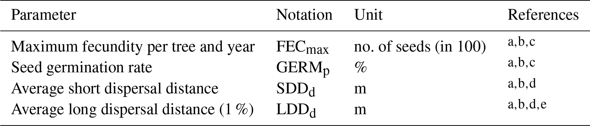
a Lischke and Löffler (2006). b TRY database (Kattge et al., 2020). c Royal Botanic Gardens Kew (2019). d Vittoz and Engler (2007). e Tamme et al. (2014). See Table B2 for species-specific range values (default, minimum, mean, maximum and percentiles) and data sources, and Table S1 for species-specific parameter uncertainties (; UI).
2.5 Evaluation of parameter uncertainty
2.5.1 Local sensitivity analysis (LSA)
As a first step, we applied a species-specific local sensitivity analysis (LSA). The LSA method quantifies the relative contribution of each parameter to the model output (first-order effect) by determining the effect of its variation on the output variability while keeping the other parameters fixed to a nominal value (Hamby, 1995). We followed the approach by Downing et al. (1985) and applied a 5-point LSA, where one parameter is adjusted to its minimum, mean, maximum, 25th, and 75th percentile values, while the others are kept at their default values (Table B2). We quantified the response of the model to each parameter in terms of directionality, linearity, and magnitude by four summary statistics: the sensitivity index (SI), two importance indexes (II1 and II2), and the linearity index (LI) (Downing et al., 1985; Hamby, 1995).
Assuming that y is the migration rate obtained by an LPJ-GM simulation and } is the vector representing the n migration parameters of the model (with n=4; see Table 2), the first-order sensitivity SIi of parameter xi is the ratio of the change of the simulated output Δy to the corresponding change in the input parameter Δxi:
where Δy and Δxi are the differences between the maximum and the minimum value of the output (ymax−ymin) and of each input parameter xi (), respectively (Downing et al., 1985). A model output that shows a large change with respect to a small parameter change is considered sensitive to that parameter, where the parameter is said to be influential. While the absolute value of SI is used to rank parameters based on the sensitivity of the model, the direction of SI (positive or negative) can help to determine whether the output is an increasing or decreasing function with regard to the individual input parameter.
The first importance index II1i is used to assess whether a large increase in the parameter uncertainty may propagate into a large uncertainty in the model output, which may be sensitive to the parameter. Thus, II1i of parameter xi is the product between its uncertainty Uxi and its effect on the model output SIi:
where Uxi is calculated as the normalized value range , where xi,max and xi,min are the maximum and the minimum values found in the literature, respectively, for each parameter xi.
The second importance index II2i is calculated as the percentage difference of the output y when varying the input parameter xi from its minimum to its maximum:
This index is useful in the case of a monotonic relationship between input parameters and output, and to account for the whole parameter range when calculating the sensitivity.
The linearity index LIi indicates whether the relationship between each input parameter and the model output approach linearity:
where s2 is the sample variance of the model output over the five points ( corresponds to the standard deviation for each parameter range, ca. ) and an exact linear relationship between model output and parameter corresponds to LIi=1. Additionally, we conducted species-specific linear regression analyses of the type y∼xi, such that every change of one parameter xi unit translates to a change of migration rate (y) given by the slope coefficient of the regression (i.e. a slope value of 1 should correspond to LIi≈1).
2.5.2 Extreme value analysis (EVA)
Having evaluated the importance of the parameters, their direction, and linearity with respect to the model output across species, we quantified the effect of species-specific parameter combinations at their extreme values on simulated migration rates. Namely, we fixed all influential parameters at their minimum (all_MIN) and maximum (all_MAX) values and calculated the corresponding errors as residuals to quantify the performance of the simulations for each species. Residuals for each species i (resi) were calculated with respect to the maximum of observational values:
where migi,sim and migi,obs_max are the simulated migration and the maximum value of migration rate estimates for species i, respectively (Table 1). Thus, residuals determine whether simulated values are over- or under-estimations with respect to observed values (i.e. positive or negative residuals, respectively, above or below 15 % of the maximum observed migration speed, where we assumed good estimates to fall within the 15 % range), and whether an error is minimized or not for each species. In other words, if the simulated migration rate is an increasing function of all parameters, outputs generated with all parameters at their minimum (all_MIN) should never exceed the upper boundary of observational values, and vice versa in the case where all influential parameters are fixed to their maximum (all_MAX). Using this insight, we tried to identify a set of parameter values to minimize residuals when possible for each species. Additionally, we conducted a Mann–Whitney U test on the residuals obtained with all_MIN and all_MAX in order to assess whether there were significant differences in model performance between the two parameter settings at the species level (via p values adjusted with Bonferroni correction for multiple comparisons).
This approach allows the exploration of the performance landscape at its extremes, thus allowing the parameter space to shrink, to some extent, while reducing considerably the number of simulations (i.e. computational demand), as EVA is independent from the number of parameters to optimize.
2.6 Evaluation of model uncertainty
2.6.1 Implementation of fat-tailed seed dispersal kernels
Following insights from our previous results (see Sect. 3.2) and recommendation from the literature (e.g. Clark, 1998; for more details see Sect. 4), we decided to implement five additional dispersal kernels to better represent LDD events in the migration model: exponential power (ExpPow), Weibull, bivariate Student's t (twoDt), logistic, log-hyperbolic secant (LogSec) (Table 3). We selected dispersal kernel functions without exponentially bounded tails (i.e. fat tails), using the exhaustive list of probability density functions provided by Nathan et al. (2012) and Bullock et al. (2017). Fat-tailed kernels are characterized by two parameters, i.e. the scale parameter a, which depends on the average dispersal distance (a1 and a2 for SDDd and LDDd, respectively), and the shape parameter b, which defines the weight of the tail. Our objective was to find the species-specific shape parameter value and kernel function that provided a better representation of the migration process (i.e. migration rate) with respect to the default negative exponential function, while keeping the remaining migration parameters within realistic values. We therefore implemented the five additional fat-tailed kernels into the dispersal sub-model of LPJ-GM and ran simulations with default parameter values for the two linearly combined probability density functions (PDFs) as calculated from the average dispersal distances at the local scale (SDDd) and for long-distance dispersal events (LDDd) (i.e. fat-tailed functions are implemented to represent the PDFs of both SDD and LDD components in Eq. A3; see Table B2 for species-specific dispersal parameter values). We varied the shape parameter b in a suitable range for each kernel, so that b values would define a mathematically significant and fat-tailed PDF (Table 3).
We evaluated the performance of the new kernels by calculating the error between simulated and observed migration rates for each species (residuals; see Eq. 5) and across species (RMSE; see Eq. 7). Additionally, we conducted a one-way ANOVA with a post hoc Tukey's HSD test among errors generated by the newly added kernels to verify whether one or more fat-tailed kernels improved the predictions across all species (RMSEs) or at the species level (residuals). Finally, we selected the kernels with significantly minimized errors for each species.
Table 3Probability density functions (PDFs) for the default dispersal kernel in LPJ-GM (negative exponential) and five additional kernels. d: dispersal distance in metres (SDDd or LDDd); a: scale parameter as a function of dispersal distance (a1 and a2 for SDDdand LDDd, respectively, in Eq. A3); b: shape parameter range to search for better representation of LDD events. Range boundaries are defined by the values for which PDF are mathematically significant and the corresponding tail is fat (Nathan et al., 2012). Table adapted from Nathan et al. (2012) and Bullock et al. (2017). Gamma function: , where n is any positive integer.

2.6.2 Uncertainty analysis
Model uncertainty is assessed with respect to model complexity, error, and sensitivity. Generally, more complex models tend to generate more accurate predictions (i.e. to minimize the error relative to observational data) by incorporating more components (e.g. parameters) into the modelling framework. However, given that each additional component may introduce sensitivity, more complex models are likely to be more sensitive too. Ideally, we would like to select a model structure where both error and sensitivity are as low as possible, i.e. where model uncertainty is minimized (Snowling and Kramer, 2001). Thus, model uncertainty can be quantified by a summary index of error and sensitivity (Snowling and Kramer, 2001):
where Ui is the utility of model i (between 0 and 1, where 1 is maximum utility), and Smax and Emax are the maximum sensitivity and error across models, where the error E is the root mean square error (RMSE; Eq. 7) between the simulated migration rates (migi,sim) and the observed values (migi,obs_max; species-specific maximum of the value ranges in Table 1). Equation 6 was derived from Eq. (3) (Snowling and Kramer, 2001) by setting the weighting constants for sensitivity and error to 1 (i.e. error and sensitivity were valued equally relative to each other in the calculation of the model utility).
where n is the number of species i, and is the average of maximum observations across species. We used the species-specific upper boundaries of the observed values since we assumed that the maximum rates detected by classic pollen analysis are good estimates of the maximum potential spread of a species under optimal climatic conditions (see Sect. 2.1).
The sensitivity S was calculated according to Eq. (3) as the mean across species and parameters. Thus, we conducted a further sensitivity analysis of minimum and maximum values for the model structure with newly implemented and best fitted fat-tailed kernels.
Additionally, we calculated an index of model complexity based on the number of parameters and processes implemented in each dispersal model structure:
where Ci is the complexity of model i, N is the number of state variables, nj is the number of processes implemented for each state variable j, pl is the number of parameters of each process i, and rl is the number of equations used to formulate each process (see Fig. A1 for a graphical representation of the components of the migration module).
We defined two different model structures relative to the phenomenological formulation of seed dispersal, which is simulated either as (1) a two-part negative exponential for all species (“Model 1: default kernel”) or (2) a two-part best-fitted fat-tailed kernel per species (“Model 2: fat-tailed kernels”). Thus, we run simulations for all species with the best set of migration parameters found by EVA for Model 1, or according to the performance analysis of the newly implemented fat-tailed kernels for Model 2. The evaluation of both indexes (Ui and Ci) should inform the choice of a model structure, which would ideally maximize its utility while not being overly complex.
3.1 Sensitivity analysis
According to the four summary statistics of the local sensitivity analysis (LSA), we identified the two most influential parameters as the mean (SDDd) and maximum (LDDd) dispersal distances for local and long-distance seed dispersal (LDD), respectively (Figs. 1 and S2). On the other hand, maximum seed fecundity (FECmax) and especially seed germination rate (GERMp) showed a smaller effect on the predictions of migration rate both across species (Fig. 1) and at the species level (Fig. S2 and Table S1). Overall, parameter ranking agreed among species, with SDDd and LDDd ranked first for 12 species, over 17 total species (Supplement Sect. 8.1.1).
All parameters related to the dispersal kernel (SDDd and LDDd) showed an overall consistency across species regarding the positive sign of their relationship with migration rate, though of different magnitude relative to the species (Figs. 1, S2 and Table S1). Magnitude-wise and on average, an increase of 1 m of mean dispersal distance for SDDd or maximum dispersal distance for LDD events leads to a corresponding increase of 0.58 or 0.30 m yr−1 of migration rate, respectively. On the other hand, maximum fecundity and germination rate had occasionally null or negative effects on the model output (Fig. S2), though the relationship was positive for most species, with an overall increase of 0.20 and 0.09 m yr−1 for each unit increase in FECmax (100 seeds) and GERMp (1 %), respectively (Supplement Sect. 8.1.2). These results were confirmed by the species-specific linearity index (LI) and slope coefficients, where values above or close to the unit indicated a strong and positive linear relationship (and thus proportional increase) of SDDd and to a lesser extent of LDDd with respect to the migration rate, whereas the sub-unit and mostly non-significant values of FECmax and especially GERMp suggested little linear relationship with the model output (see Fig. 1 and Table S1 for LI values, and Figs. S2 and S3 for species-specific slope coefficients and species-specific shapes of sensitivity functions, respectively).
Uncertainty in parameter estimates from literature sources seemed to be highly species-specific (Table S1), though overall FECmax and GERMp showed the highest and the lowest uncertainties, respectively. The effect of parameter uncertainty on simulated migration rates (II1) was overall greater for SDDd due to the large sensitivity of the model output to this parameter (Fig. 1), though the uncertainty of SDDd is moderate with respect to others (52.70±41.06; Supplement Sect. 8.1). On the other hand, the relatively high effect of FECmax on migration rate (II2) was mainly due to its high uncertainty (3470.82±9339.38; Supplement Sect. 8.1), especially in the case of Betula spp. (28 275), Carpinus betulus (682), and Ulmus glabra (894) (Table S1). Similarly, the higher importance of LDDd when accounting for the whole parameter range (II2) seems likely due to the large uncertainty associated with estimates of maximum dispersal distances (Table S1).
In summary, parameters linked to the seed dispersal kernel appear to be the most influential, while as expected all parameters are overall positively related to migration rate over the range of each individual parameter for most species (see Sect. 2.2). Insights gained from the LSA and from the equations of the migration module (see Sects. 2.2 and 4, and Appendix A) indicate that the migration function is also monotonic over the entire parameter space, at least in the neighbourhood of the default values. Thus, we expect that by increasing the values of all parameters within acceptable ranges for each species, simulated migration rates will correspondingly increase to their potential maxima.
We applied this insight to the extreme value analysis (EVA).
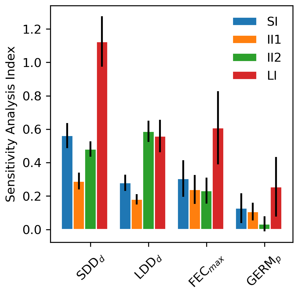
Figure 1Mean sensitivity analysis (SA) indices (±2 standard errors) across 17 tree species for the four parameters of the newly implemented migration module of LPJ-GM: average short dispersal distance (SDDd, m), 1 % average long dispersal distance (LDDd, metres), maximum fecundity per tree (FECmax, no. of seeds per 100 yr), and seed germination rate (GERMp, %). See Sect. 2.5.1 for the calculation of SA indices: sensitivity index (SI), importance indexes (II1 and II2), and linearity index (LI). See Table S1 for species-specific values.
3.2 Extreme value analysis
Species-specific residuals between simulated migration rates and maximum observed values, where migration parameters were varied simultaneously to their minimum (all_MIN) or maximum values (all_MAX) per species, is shown in Fig. 2. Negative residuals indicate that model outputs underestimate historical observations across all species, with the exception of the over-estimations obtained with the all_MAX setting for Abies alba and Picea abies (>15 % from the maximum observed migration speed; Fig. 2, Table S2, and Supplement Sect. 8.2.3). Consequently, we looked for smaller parameter values (all_MAX_opt) to minimize the error for both species (RMSEall_MAX_opt=1.67 % vs. RMSEall_MAX=233.33 % for Abies alba, and RMSEall_MAX_opt=1.80 % vs. RMSEall_MAX=95.20 % for Picea abies; Table S2 and Supplement Sect. 8.2.4).
Overall, simulated migration rates showed high errors with respect to the maximum of observational data for both extreme value settings, though migration rates generated by all_MAX were significantly less biased than estimates generated by all_MIN (Mann–Whitney U test and Bonferroni adjusted p value ), both across species (RMSEall_MIN=109.0 %; RMSEall_MAX=96.79 %; Supplement Sect. 8.2.2) and at the species level, with the exception of Pinus halepensis (p value =1.0) and Quercus pubescens (p value =0.04; see Supplement Sect. 8.2.1 for all species-specific p values).
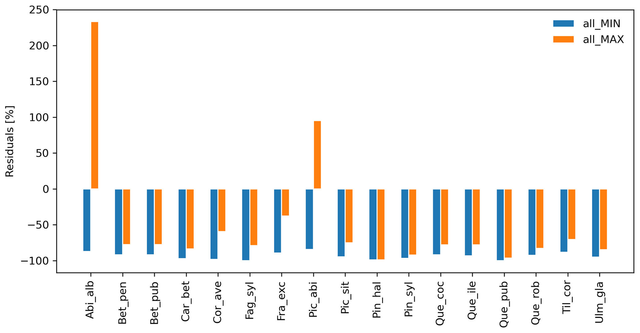
Figure 2Species-level residuals of observed versus predicted migration rates for extreme parameter settings. The observed migration rates refer to the maximum value of historical estimates (upper boundaries of migration rates in Table 1; Eq. 5). all_MIN: all migration parameters are fixed to their minimum values; all_MAX: all migration parameters are fixed to their maximum values. See Table B2 for species-specific extreme parameter values, and Table S2 for species-specific residuals.
3.3 Performance of fat-tailed kernels
Newly implemented fat-tailed kernel functions with examples of shape parameter b values and scale parameters a based on the same LDD and mean dispersal distance data are shown in Fig. 3, compared to the default negative exponential. Exploring the species- and kernel-specific parameter space of the shape parameter while keeping the remaining migration parameters within realistic values (see Table 2), we found that overall simulated migration rates over-estimated maximum observed values when generated by the logistic function in the shape parameter range [3–4], and by the log-hyperbolic secant and twoDt functions around the 0.5 and 2 values, respectively (Fig. 4). On the other hand, the exponential power function at lower b values [0.15–0.3] and the Weibull function across the whole parameter range selected [1.75–2.5] tended to under-estimate observed values (Fig. 4).
After selecting the best shape parameters per kernel (i.e. yielding the minimum residual; Table S3), we confirmed that the Weibull function under-estimated observed migration speed across all species, whereas the log-hyperbolic secant and logistic functions were overall the best at minimizing residuals at the species level (Fig. 5). Nevertheless, we found significant differences in kernel performance based on the species (Figs. 5, 6, Table S4, and Supplement Sect. 9.4.3). For example, the exponential power function generated good estimates for Corylus avellana (RMSE =25.75 %), while the logistic and log-hyperbolic secant functions tended to over- and under-estimate, respectively, migration rates by ≈20 %. Conversely, good estimates of migration rates for Quercus spp. were generated by the logistic and log-hyperbolic secant functions (RMSE ≈1 %–15 %), while the exponential power function produced under-estimations across the whole range of observed values by ≈90 % (Supplement Sect. 9.4.3).
Overall, fat-tailed kernels were able to significantly improve model outputs relative to the default negative exponential both across species and at the species level, with the exception of Abies alba and Picea abies (see Sect. 3.2). Concerning the worst performances at the species level, the simulated migration rate obtained with the default kernel had higher error relative to the observed maximum value (RMSE =98.93 % for Pinus halepensis) compared to the significantly less biased estimate generated by the logistic function (14.67 %) (Supplement Sect. 9.4.4). Kernel functions can be ranked based on RMSE % calculated across species as follows: (1) log-hyperbolic secant (17.73 %), (2) logistic (31.70 %), (3) twoDt (49.81 %), (4) exponential power (76.90 %), (5) negative exponential (92.81 %), and (6) Weibull (99.90 %) (Supplement Sect. 9.4.1). Finally, we selected the kernel function that significantly minimized residuals for each species as shown in Fig. 6 (see Table B3 for species-specific values of all optimal parameters).
Additional simulations with optimized parameters that tested alternative competitors (apart from Betula spp.) showed that migration rate is relatively robust to different competitors. For the three species tested with alternative competitors, the error between simulated migration speed and observed maximum value had a small increase, while staying below the threshold of good estimates (RMSE <15 %; Sect. 2.5.2): Fagus sylvatica (from 5.3 % to 14 % with Quercus robur), Picea abies (from 1.8 % to 11.8 % with Pinus sylvestris), and Tilia cordata (from 3.2 % to 3.6 % and 10.4 % with Pinus sylvestris and Quercus robur, respectively; Supplement Sect. 9.5). Similarly, the overall error of the model had a minor increase (from 7.7 % to 8.13 %) and the model utility stayed constant (0.58) (cf. Sect. 3.4). Regarding the influence of the dispersal patch size, our parametrization holds for the spatial resolution of 1 km (with a finer resolution of 100 m for the simulation of the dispersal kernel) (see Sect. 2.3).

Figure 3Probability density functions for the newly implemented fat-tailed seed kernels. Fat-tailed kernels with examples of shape parameter values are compared to the default negative exponential (NegExp). Newly implemented kernels are as follows: ExpPow: exponential power; Weibull; twoDt: bivariate Student's t; logistic; LogSec: log-hyperbolic secant. See Table 3 for the kernel formulae and range values of the shape parameter for each kernel. Kernel formulae are implemented as PDFs in Eq. (A3) for both the SDD and LDD component. The 2D dispersal patch size (maximum dispersal distance) is 500 m (which corresponds to seeds dispersing from the centres of 1 km2 cells as in the default spatial configuration of LPJ-GM), with SDDd and LDDd set to 100 and 500 m, respectively. Dispersal probabilities of each kernel are scaled in the [0–1] range for comparison.
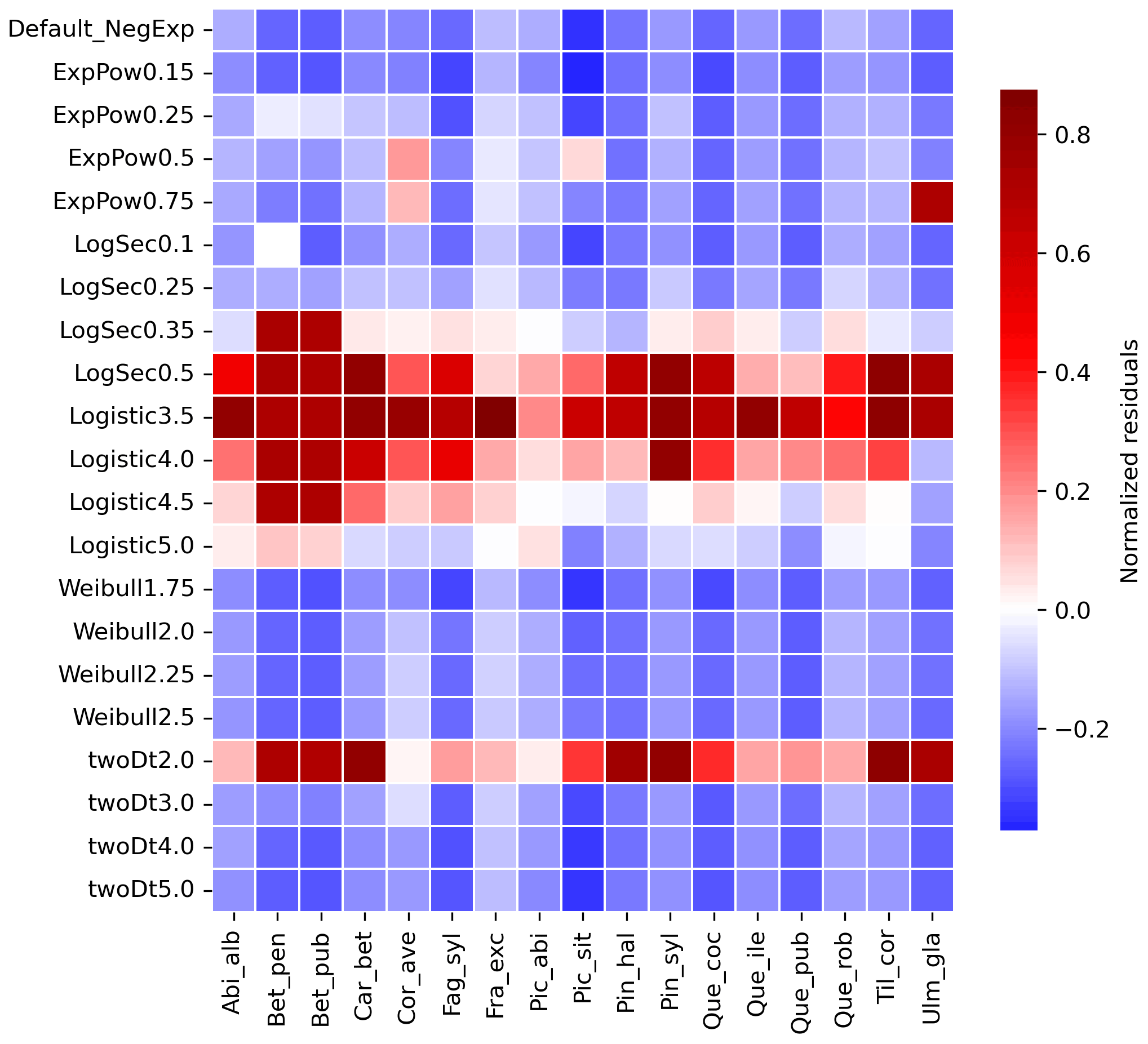
Figure 4Species-specific performance of seed kernels for different shape parameters. The heat map shows the species-specific normalized residuals between simulated migration rates and observed maximum historical estimates for the default negative exponential function (“Default_NegExp”) and the newly implemented fat-tailed kernels across examples of shape parameter values (“{ kernel name} +{b value}”; cf. Fig. 3). Red and blue indicate over- and under-estimations, respectively. See Table S3 for species- and kernel-specific residuals and simulation values for all tested shape parameter values.
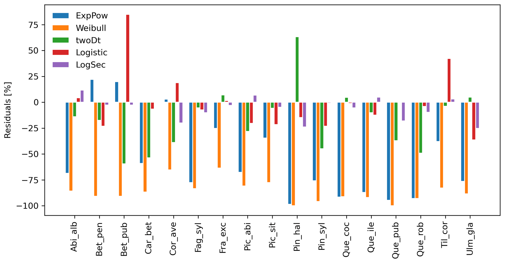
Figure 5Performance evaluation of fat-tailed kernels. Comparison of species-specific residuals of observed versus simulated migration rates among newly implemented kernel functions. Observed values corresponds to the maximum of historical estimates (Table 1; Eq. 5).
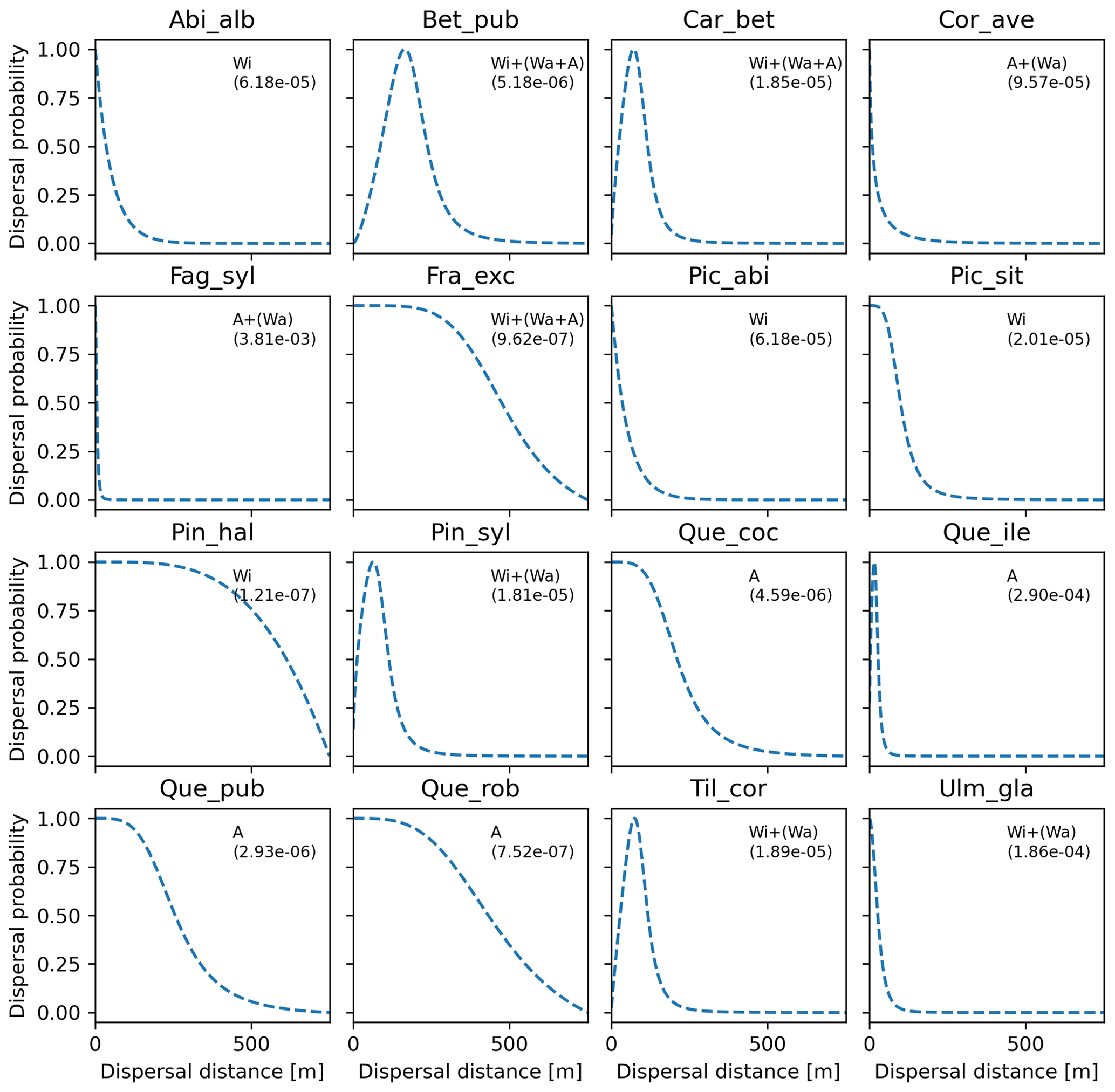
Figure 6Best fat-tailed kernel shapes per species. See Table B3 for the corresponding parameter values: kernel function, SDDd, LDDd, and shape parameter b. Each species-specific kernel function is implemented as PDF in Eq. (A3) for both the SDD and LDD component. Dispersal probabilities of each kernel are scaled in the [0–1] range for comparison. Maximum values of unscaled probabilities are indicated in parentheses. Species-specific dispersal mechanisms: Wi: wind; Wa: water; B: bird; A: animals, with secondary mechanisms in parenthesis (Table B1).
3.4 Uncertainty analysis
The results of the analysis of model uncertainty for the two modelling frameworks – seed dispersal simulated either with a negative exponential kernel across species (Model 1: “default kernel”) or with species-specific fat-tailed kernels (Model 2: “fat-tailed kernels”) – are shown in Fig. 7.
Model complexity is calculated from four processes – (1) seed production, (2) seed dispersal, (3) seed bank dynamics, and (4) seedling establishment – represented by one operation each, including (1) FECmax, (2) SDDd and LDDd, (3) GERMp, and (4) GERMp for Model 1 (), and (1) FECmax, (2) SDDd, LDDd and b, (3) GERMp, and (4) GERMp for Model 2 (), respectively (see Appendix A and Fig. A1). Thus, the added unit of complexity for Model 2 results from the inclusion of the shape parameter b as weight for the fat-tailed kernels.
Confirming previous error analyses at the species level (Sect. 3.3), the use of fat-tailed kernels managed to reduce model error by ≈85 % across species compared to the default setting (RMSE1=92.81 % vs. RMSE2=7.70 %). As expected from theory (Snowling and Kramer, 2001; see also Sect. 2.6.2), model sensitivity increased along with complexity, with Model 2 being nearly 2 times more sensitive across all its parameters than Model 1 (S1=0.27 vs. S2=0.42). This was mainly due to the inclusion of the shape parameter for fat-tail kernels in Model 2 (b), to which the model output is highly sensitive (Fig. 7). On the other hand, the ranking of parameters based on their effect on simulated migration rates is the same for both model structures, with dispersal distances for local (SDDd) and long-distance dispersal (LDDd) being the most influential parameters. Comparing parameter effects among the two model structures, simulated migration rates were more sensitive to germination rates (GERMp) in Model 2 relative to Model 1, whereas SDDd was more influential in Model 1 relative to Model 2 (Fig. 7).
Overall, the inclusion of fat-tailed kernels improved model utility to a moderate level, U2=0.58 (where U=1 is the ideal model utility), with respect to the default modelling framework (U1=0.34).
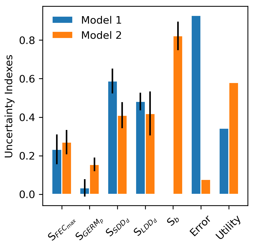
Figure 7Comparison of parameter-specific sensitivities, model error and utility between two structures of the migration module of LPJ-GM. Model structures refer to seed dispersal simulated either with a linear combination of two negative exponential kernels across species (Model 1: “default kernel”) or of species-specific fat-tailed kernels (Model 2: “fat-tailed kernels”) (see Eq. A3). Sb: model sensitivity to the shape parameter b of fat-tailed kernels (see Table 2 for the description of other parameters). Note that the kernel formulation of Model 1 has no shape parameter (hence, Sb is NA). See Sect. 2.6.2 for the calculation of model utility.
The sensitivity analysis (SA) classification showed that migration rates had lower sensitivity to local demographic traits (germination rate and maximum annual fecundity) than to parameters related to seed dispersal (average distance for local dispersal and rare LDD events) for most of the species (Fig. 1 and Table S1). Similar results were found by two studies applying SA on mechanistic models for the simulation of seed dispersal (Soons et al., 2004; Nathan and Katul, 2005). In both cases, average dispersal distances or LDD were more influenced by parameters linked to the dispersal kernel (e.g. horizontal wind velocity) than to local demographic or environmental factors. The importance of dispersal parameters was also confirmed by the study of Lustenhouwer et al. (2017) on the relationship between dispersal ability, local demographic traits, and migration speed across 80 plant species, including trees. Lustenhouwer et al. (2017) found that the intrinsic migration capacity of tree species (simulated by the Clark et al., 2001 model) was significantly and positively correlated to dispersal ability (i.e. decreasing rate of dispersal as a function of distance from the mother tree). On the other hand, local demographic traits such as fecundity had a weaker correlation to spread velocity (Lustenhouwer et al., 2017). Our metrics of the shape between migration rates and migration parameters (LI in Fig. 1 and slope coefficients in Fig. S2) further highlighted a linear effect of dispersal distances (especially for local dispersal) on migration rate, whereas maximum fecundity and germination rate seemed to affect migration in a bounded way (see also Fig. S3). Similar shapes were found by Lustenhouwer et al. (2017) when analysing the relationship of spread velocity with dispersal ability (linear) and fecundity (asymptotic). The shape of our relationships can be explained by the formulation of the migration process in the model LPJ-GM and the calculation of migration rates. Migration speed is defined by the distance of an individual from the migration source (i.e. mother tree) when surpassing a certain leaf area index threshold (LAI =0.5) and accounting for the time elapsed since the start of migration (see Sect. 2.2 and Appendix A). In turn, individual biomass at a location depends on the number of seeds produced by the individual each year (i.e. annual fecundity), by the distances at which seeds are dispersed (i.e. seed dispersal kernel described by SDDd and LDDd) and by the local biomass growth. On the one hand, annual fecundity and biomass growth are determined by environmental conditions, and inter- and intra-specific competition for light and space. Thus, we expect that the positive effect of maximum fecundity on migration rate will form a plateau when species reach their carrying capacity at a site. On the other hand, an increase in average dispersal distance would likely translate into an almost direct (i.e. linear) increase in migration speed, which corresponds to seed movement per time unit.
The overall increase in migration rate values given by simultaneously setting all parameters to their maximum values (all_MAX) supported our assumption that the simulated migration rate is likely an increasing function of the four migration parameters. However, high and significant error values corresponding to all_MAX simulations suggested that the default model structure was unable to generate unbiased estimates within the acceptable range of parameter values for most species, with the only two exceptions being Abies alba and Picea abies (Fig. 2). This systematic underestimation might indicate that an ecological process significant to tree migration is missing or is incorrectly represented by the default model structure. In this respect, a number of studies on plant migration modelling suggests that the asymptotic behaviour of the dispersal function (i.e. the extent of the tail) is crucial for the simulation of population spreading rates, where kernel tails represent LDD events (Clark, 1998; Caswell et al., 2003). Our default model implements LDD events in the weighted linear combination of two negative exponential functions that represent SDD and LDD events with a 0.99 and 0.01 relative probability, respectively. However, dispersal kernels with high kurtosis and long or even fat tails (i.e. not exponentially bounded) are generally considered more accurate representations of LDD events than negative exponential functions (Clark et al., 1999; Bullock and Clarke, 2000; Nathan et al., 2012), especially in the case of species with a high probability of LDD due to the presence of active dispersal vectors, such as hoarding or migratory animals (Clark, 1998; Clark et al., 1999; Powell and Zimmermann, 2004). This is in agreement with our species-specific best performance across seed kernels relative to the natural dispersal syndrome of the tree species (Tables B1 and B3). Specifically, the only two species that could generate unbiased estimates of migration rates with the default negative exponential function (Abies alba and Picea abies) are primarily dispersed by wind, a passive dispersal vector. On the other hand, fat-tailed kernels provided a better fit for animal- or wind-dispersed species with additional LDD mechanisms, such as water currents and migratory animals (e.g. birds; see Schurr et al., 2009, for a classification of LDD mechanisms). Overall, wind-dispersed species tended to have higher maximum dispersal distances than species primarily dispersed by animals (Fig. S4), in agreement with observational studies on vegetation spread in temperate and tropical forests (Clark et al., 1999). From an ecological point of view, this can be explained by the average traits of wind-dispersed seeds, which are smaller and winged and thus more likely to be transported farther compared to the heavier animal-dispersed seeds. From a modelling point of view, larger LDD values would allow the simulation of high migration rates even with an exponentially bounded kernel function. On the other hand, animal-dispersed species might have shorter dispersal distances on average (Fig. S4) but can potentially reach higher migration rates via rare LDD events producing outlying individuals ahead of the migration front. In this case, the use of fat-tailed kernels will produce a noisy and accelerating vegetation spread relative to a step-wise and slower spreading front given by exponentially bounded kernels (Clark, 1998). This seems to suggest that occasional LDD events are more important for tree migration than local dispersal driven by more common vectors, at least in order to achieve the spreading rates of the paleo-records used in this study. Supporting this, dendrochronological analyses of subfossil stumps have shown that the mid-Holocene expansion of P. sylvestris into northern Scotland likely progressed by LDD events with initial immigration by very few individuals followed by infilling after a delay (possibly by the mature progeny of the first colonizers), rather than by a step-wise migration front (Gear and Huntley, 1991; Daniell, 1992, 1997; Huntley et al., 1997). Similarly, previous modelling studies showed that migration rates generated by fat-tailed kernels are more compatible with historical estimates of post-glacial forest expansion than rates obtained with Gaussian-like kernels or other functions that poorly represent LDD events (Cain et al., 1998; Caswell et al., 2003). The importance of LDD in post-glacial tree expansion has been long recognized as the most likely explanation to the Reid's paradox, i.e. the apparent discrepancy between contemporary plant dispersal potential and observed post-glacial migration rates (Reid, 1899; Cain et al., 1998). In the context of the Reid's paradox, dispersal potential mostly refers to the common (99 % of events) SDD relying on conventional dispersal vectors, whereas high post-glacial migration rates are explained by rare (1 %) LDD events where trees colonized newly emptied areas via less common vectors (e.g. water or a large or migratory animal) (Higgins et al., 2003b; Vittoz and Engler, 2007; see also Sect. 4.4 of Birks, 2019, for a discussion of possible scenarios of post-glacial forest expansion).
The shape of the kernel tail can affect not only the migration speed but also its sensitivity to other migration parameters. In agreement with Clark (1998), the implementation of fat-tailed kernels enhanced the importance of ecological traits linked to migration, especially germination rate, compared to negative exponential kernels (Fig. 7). Additionally, relatively small differences in the tail shape of fat-tailed kernels (i.e. shape parameter) had strong effects on the migration rates (Figs. 4 and 7). Such a high sensitivity might add to the uncertainty of parameter estimates and thus lower the confidence of model predictions with fat-tailed kernels. However, it might be observed that the tail shape is inherently uncertain, regardless of the kernel function used. That is, we cannot reliably fit the tail to empirical data of LDD and shape parameters as these are nearly impossible to estimate with high accuracy, especially in the case of animal-dispersed species (Clark et al., 2003). For example, compared to the relatively easier recovery of seeds from traps for wind-dispersed species, it would be required to know in advance which animals would act as dispersal vectors and then visually follow or track them until seeds are deposited on the ground (Beckman et al., 2020). Furthermore, it has been observed that a single dispersal probability density function cannot be standardized for all species since kernel shapes depend on species-specific dispersal mechanisms (Bullock et al., 2017). At the same time, a kernel shape cannot be built based on a specific dispersal mechanism as a given species can disperse using a variety of vectors (Nathan et al., 2008; Counsens et al., 2018). Under these considerations, our approach was to implement species-specific dispersal kernels that summarized dispersal modes (see “total dispersal kernel”; Nathan et al., 2008) and provided a good representation of LDD events that could match the historical spreading rates, rather than find the kernel function that best-fitted experimental data of seed shadows.
Overall, our results seem to justify the use of simple functions to summarize multiple dispersal modes and simplify complex dispersal mechanisms, at least in a large-scale context. For example, in the case of continental-scale simulations over thousands of years (e.g. post-glacial forest expansion), it is suggested to avoid a more detailed representation of migration that would require the inclusion of, for example, wind properties, animal movement and behaviour, seed retention and deposition. Such local stochastic processes are generally challenging to parametrize in models given the difficulty of observation and their case-specific nature (Nathan et al., 2012). As such, the choice of species-specific phenomenological dispersal functions would allow a reduction in the inherent uncertainty of migration models compared to more explicitly mechanistic representations of seed dispersal, while still providing a representation of dispersal abilities and population dynamics (via germination rates and maximum fecundity) at the species level.
There are a number of reasons for the disagreement between model output and observations besides parameter and model uncertainties.
Observational range values of migration rates and/or of migration parameters obtained from the literature might be incorrect or too uncertain.
We decided to simulate the spread of tree species across a homogeneous terrain (for permeability) and non-limiting climate in order to reduce as much as possible the effect of the environment on the simulated migration rates. This allows of the impact of parameters and model structure to be assessed, a comparison among species with equal simulation settings to be conducted, and migration parameters to be optimized to match maximum migration speeds from the literature (as we assume that a non-limiting climate may allow species to achieve the maximum potential spread recorded by paleo-records; see Sect. 2.1).
As an avenue of future research, settings with heterogeneous terrains and climate can be applied to simulations to assess the relative contribution of climate, landscape heterogeneity, habitat loss, and dispersal ability in the context of real-world scenarios. For example, a simulation of major tree taxa across the different habitats of Europe and for the last 20 000 years of changing climate may give some insights into the prevalence of migration lag among the simulated species (i.e. the delayed arrival of a species into a newly suitable habitat) during the post-glacial forest expansion (Normand et al., 2011; Svenning and Sandel, 2013; Sect. 4.4 of Birks, 2019). For a more explicit assessment of landscape configuration on species' range shifts, future simulations can be performed by driving LPJ-GM with projections of climate and land use change throughout the whole 21st century, as human-driven habitat loss has already been reported to have significantly affected plant migration at the start of the current century (Guo et al., 2018). In this regard, LPJ-GM can optionally simulate heterogeneous landscapes by using a spatially explicit seed dispersal permeability value (Lehsten et al., 2019), where landscape permeability can be informed by future projections of land use change.
We assumed static parameters, whereas, for example, germination rate is usually dependent on temperature and light regimes (Baskin and Baskin, 1998). Though there are some instances of evolutionary responses concerning dispersal ability (e.g. adaptation to the new environment may reduce the need to disperse), these are more prevalent among short-lived organism such as insects (De Meester et al., 2018). As long-lived perennials, trees seem to have a slow plastic or evolutionary response with respect to other taxa and are more likely to respond to climate change with range shifts (Berg et al., 2010; Lenoir et al., 2020; see also Sect. 6.3 and Table 11 of Birks, 2019, for the little evidence of plasticity or adaptation of terrestrial plants during the Quaternary).
We did not conduct a formal and thorough model calibration by using an optimization algorithm, though we have still identified valuable parameter estimates (i.e. we minimized the error by staying within probable parameter combinations) and helped to reduce the parameter space (following the concept of exploratory landscape analysis; Mersmann et al., 2011; Stork et al., 2020). A thorough optimization could be the next step and might suggest whether there is more than one local optimum (global optimization; Stork et al., 2020). However, these approaches are very expensive for complex models such as LPJ-GM. Furthermore, obtaining a better fit to observations does not necessarily guarantee that a model is more realistically simulating vegetation dynamics (i.e. right predictions for the wrong reasons). Uncertainty assessment is still useful to identify model components to improve (e.g. parameter uncertainty to reduce by acquiring more empirical data). More generally, our efficient uncertainty assessment could be used to reduce the cost of solving optimization problems for computationally demanding models by allocating computational resources on relevant model components (parameters or process formulations) and gain insights into model limitations for further improvement.
Predicting future trees' range shifts based on a model parametrized with early- and mid-Holocene estimates might present some limitations since past and current global warming have different intensities and species are submitted to different conditions (e.g. habitat loss, decrease in natural dispersal vectors such as large mammals or birds, and increase in human-driven dispersal in present and future conditions with respect to the early- and mid-Holocene; Corlett and Wescott, 2013; see also Sect. 7.2.2 and 7.2.3 of Birks, 2019). Nevertheless, the outcome of our study is important not in the sense that post-glacial migration estimates are to be expected in the future, but rather that we implemented important mechanisms controlling migration rate (LDD events) into the model structure (fat-tail kernels) (Nogués-Bravo et al., 2018). The high velocity of isothermal shift predicted for the 21st century (up to 4–6 km yr−1; Svenning and Sandel, 2013; Lenoir et al., 2020) suggests that trees will be limited by their dispersal ability (i.e. migration lag), and especially by LDD events in landscapes where the availability of suitable habitats has been severely decreased by human activities. Thus, the model representation of LDD will likely be more important for the realistic simulation of future range shifts.
Model predictions of species range shifts have many sources of uncertainties, which is important to acknowledge and evaluate as a first step for model improvement. This study aimed to provide an evaluation of the parameter and model uncertainties of the migration module of a dynamic vegetation model, LPJ-GM 1.0. We used low-cost methodologies for estimating the sensitivity of one model output, tree migration rate, to key migration parameters and provided quantitative information about the importance of mechanisms underlying the migration process across different tree species and a first guess of parameter values used in the simulations. Overall, the model structure implementing fat-tailed dispersal kernels provided significantly better predictions than the default modelling framework, while not being overly more complex, and can therefore be a good candidate for an improved model structure (LPJ-GM 1.1). Though a reduced model error does not necessarily mean that predictions of migration rates would be correct, the efficient inclusion of influential migration mechanisms (LDD events) in the model structure (via fat-tail kernels) can improve our confidence in range shift predictions, especially in a context of global change where LDD will likely be more relevant.
For more details on the model description and technical implementation, see Lehsten et al. (2019). See also Fig. A1 for a graphical summary of the migration module.
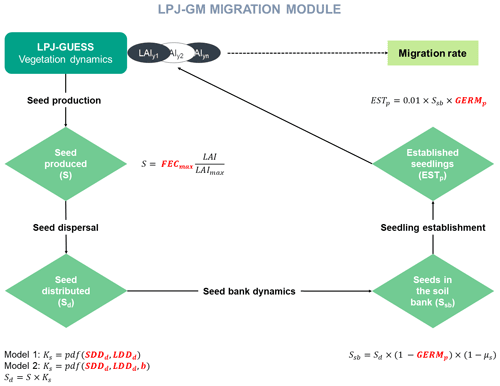
Figure A1Migration module of the model LPJ-GM 1.0. Migration consists of four processes: (1) seed production, (2) seed dispersal via a probability density function (PDF, dispersal kernel), (3) seed bank dynamics, and (4) seedling establishment. Migration parameters are highlighted in red. Model 1 and Model 2 refer to the default and modified model structures employing negative exponentials or species-specific fat-tailed kernels, respectively, for seed dispersal (see Sect. 2.6.2).
A1 Seed production
The number of seeds produced S is the product of maximum fecundity (FECmax) and the proportion of current leaf area (LAIind) to the maximum (LAImax, calculated following Eqs. 3.20 and 3.21; Bugmann, 1994):
where species-specific LAIind is generated yearly for each simulated tree individual by the main vegetation dynamic model (LPJ-GUESS).
A2 Seed distribution
The seeds produced at a location are distributed according to a probability density function (PDF), i.e. the seed dispersal kernel ks, so that the seed input Sd(xy) in location x, y is obtained by integrating over all other locations x, y:
The dispersal kernel ks is a linear combination of two PDFs for short- (SDD) and long-distance dispersal (LDD):
where LDDp is the proportion of long-distance dispersal (the actual value is species dependent; for example, LDDp of Fagus sylvatica corresponds to 0.01, i.e. 1 % of seed dispersal is attributed to long-distance transport), a1 and a2 are the scale parameters calculated from SDDd and LDDd, respectively (the average distances for SDD and LDD; see Table 3), b is the shape parameter defining the weight of the tail, and is the distance between a sink cell (xy) and a source location (xy).
In the default setting of LPJ-GM (“Model 1: default kernel” according to the model uncertainty analysis; Sect. 2.6.2), the PDFs for both SDD and LDD components are negative exponentials. In the modified model structure (“Model 2: fat-tailed kernels”; Sect. 2.6.2), the PDFs for both SDD and LDD components are species-specific fat-tailed kernels (see Table 3 for PDFs' formulae).
A3 Seed bank dynamics
The seed bank dynamic is defined by the yearly change of dormant seeds in the soil Ssb that can germinate in the following years. Ssb increases by the seed input Sd according to Eq. (A2) and decreases by the number of germinated seeds or by loss of seeds (μs):
with
where GERMp is the rate of germination, and the yearly loss of seeds from the seed bank μs is 0.8.
A4 Seedling establishment and calculation of migration rate
Finally, the probability of seedling establishment in a certain year ESTp depends on the number of available seeds for germination (Ssb) and on the germination rate:
New individuals are then established as saplings, where sapling numbers correspond to the rounded value for ESTp. The established seedlings grow, compete, and die according to the LPJ-GUESS algorithm, and finally start producing seeds following Eq. (A1).
At the end of the simulation, the species-specific migration rate (in m y−1) is calculated as the migration distance divided by migration time, i.e. the simulation time elapsed since the end of the spin-up phase when the vegetation, soil, and litter pools develop from “bare ground” into a dynamic equilibrium. During this phase, all simulated species (i.e. the focal migrating species and its competitors; see Table 1) are allowed to establish without seed limitation, whereas migrating species are killed at the end of the spin-up phase throughout the simulation domain, with the exception of the starting point of migration. Migration distance is then obtained by the direct output of LPJ-GM, yearly and species-specific leaf area index (LAI), as the distance between the starting point of migration and the 95th percentile farthest point in the terrain where LAI exceeds 0.5.
A5 Methods to enhance dispersal simulations
LPJ-GM implements (1) the fast Fourier transform method (FFTM) to enhance the computational efficiency of dispersal simulations and (2) the use of corridors to reduce the spatial domain of simulations (i.e. number of grid cells where local dynamics are simulated). The FFTM employs the convolution theorem and the fast Fourier transform (FFT) to evaluate the convolution of seed production and dispersal kernel (Eq. A2) at reduced computational cost, while allowing for the inclusion of different species-specific dispersal kernels and thus potentially dispersal syndromes (e.g. via wind or animal transport).
The dispersal syndromes and migration parameters were compiled from various literature sources (Tables B1 and B2, respectively) as described in Sect. 2.4. Optimal values (i.e. corresponding to minimized errors between predicted and observed migration rate estimates) are listed in Table B3.
Table B1Species-specific dispersal syndromes as reported by the TRY Database (Kattge et al., 2020) and supporting literature. TRY Database was searched for the plant trait “Dispersal syndrome” (TraitID: 28) for each species listed in the table (species IDs: 29, 7356, 7359, 2710, 202255, 10773, 14688, 23906, 25247, 41907, 41942, 42185, 42129, 45348, 45402, 45465, 45470, 54325, 55452, 236496, 236497, 31578, 254407, 254408). Dispersal syndromes were then grouped based on the dispersal mechanism: anemochory (dispersal by wind, Wi), hydrochory (dispersal by water, Wa), zoochory (dispersal by animals on the body surface or via ingestion). Zoochory was further divided to identify the animal vector of dispersal with support by research papers (references): B: bird; LA: large mammal (deer, badger, cattle); SA: small animal (e.g. hoarding by rodents). Next, the occurrence and the percentage of each dispersal group were calculated for each species.
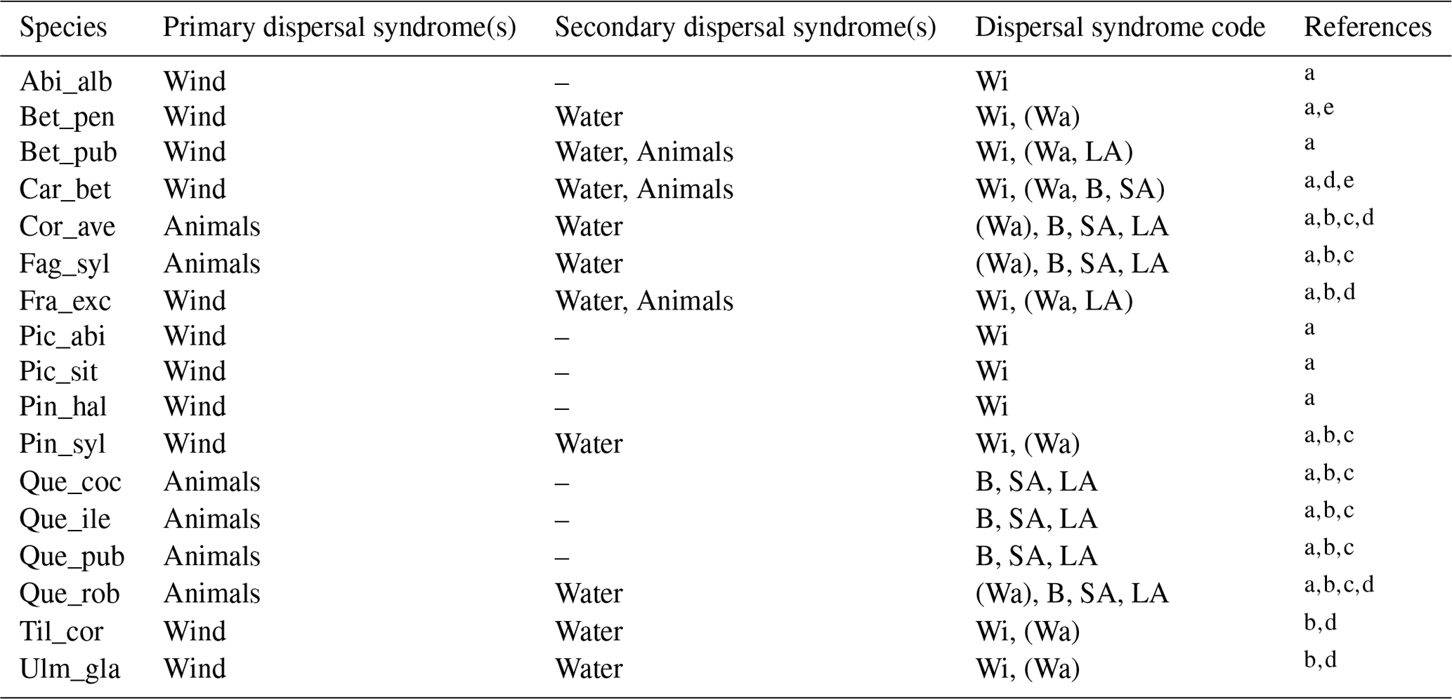
We classified a dispersal syndrome as a secondary mechanism in case its percentage of occurrence was <30 % with respect to other dispersal syndromes, with further support by research papers: a Vittoz and Engler (2007). b Wilkinson (1997). c Giannakos (1997). d Chećko et al. (2015). e Lovas-Kiss et al. (2018). We excluded mechanisms which accounted for <5 % of dispersal syndromes.
Table B2Species-specific migration parameters and data sources for minimum and maximum values found in the literature. SDDd: average short dispersal distance (metres); LDDd: 1 % average long dispersal distance (metres); FECmax: maximum fecundity per tree (no. of seeds per 100 yr); GERMp: seed germination rate (%).
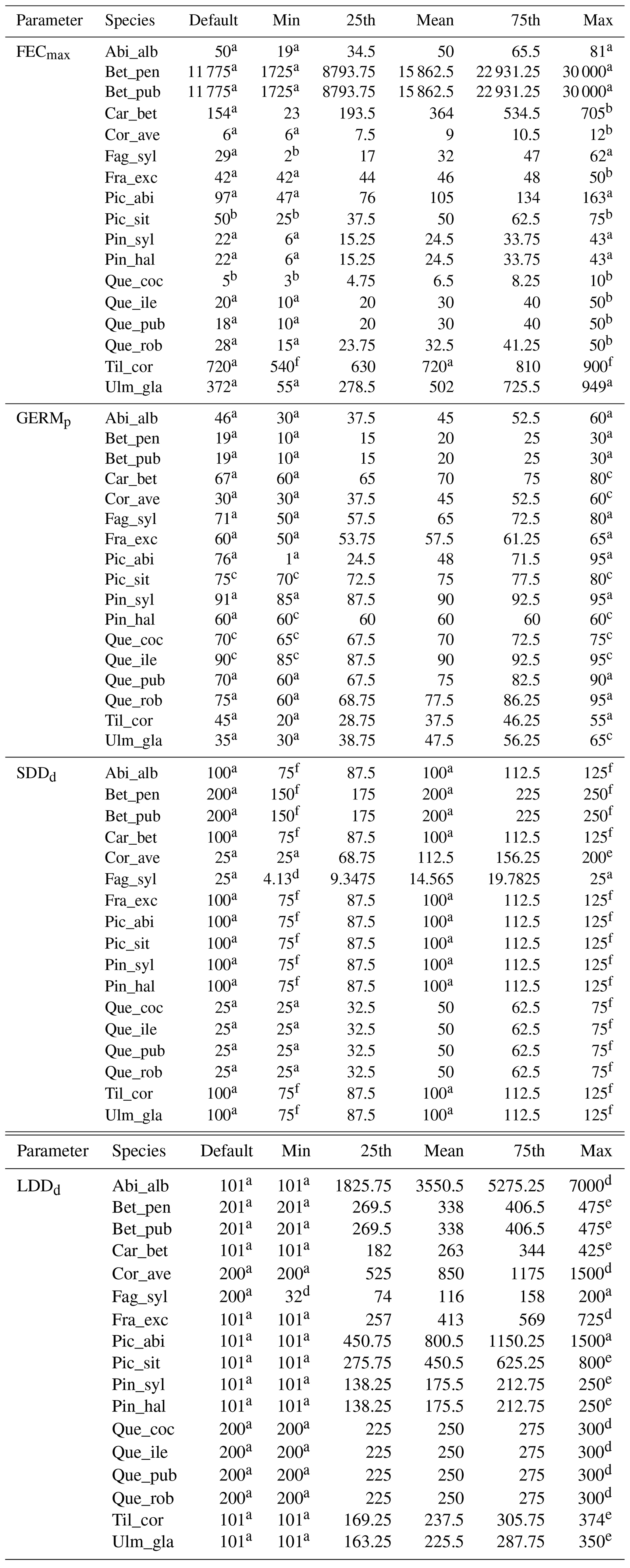
Data sources: a Lischke and Löffler (2006). b TRY database (Kattge et al., 2020). c Royal Botanic Gardens Kew (2019). d Vittoz and Engler (2007). e Tamme et al. (2014). f Species-specific variation of the 5-point parameter values is set at 12.5 % when data are lacking (e.g. for SDD, with a parameter range of 100, 25–125 m; the difference between each of the adjacent LSA-5-points is 12.5 m; see Sect. 2.4). Note that differently from the source literature for the default setting (Lischke and Löffler, 2006), we assumed the proportion of LDD events to be fixed at 1 % (LDDp=0.01). In the case of absence of LDD events (k=0 according to Lischke and Löffler, 2006), we assumed equal values for average short and long dispersal distances (SDDd=LDDd).
Table B3Species-specific optimal migration parameters with related RMSE % (relative to the maximum value of historical estimates; see upper boundaries in Table 1) and dispersal syndromes as reported by the TRY Database (Kattge et al., 2020) and supporting literature (see Table B1): Wi: wind; Wa: water; B: bird; LA: large mammal (deer, badger, cattle); SA: small animal (e.g. hoarding by rodents). Secondary mechanisms of dispersal are in parenthesis.
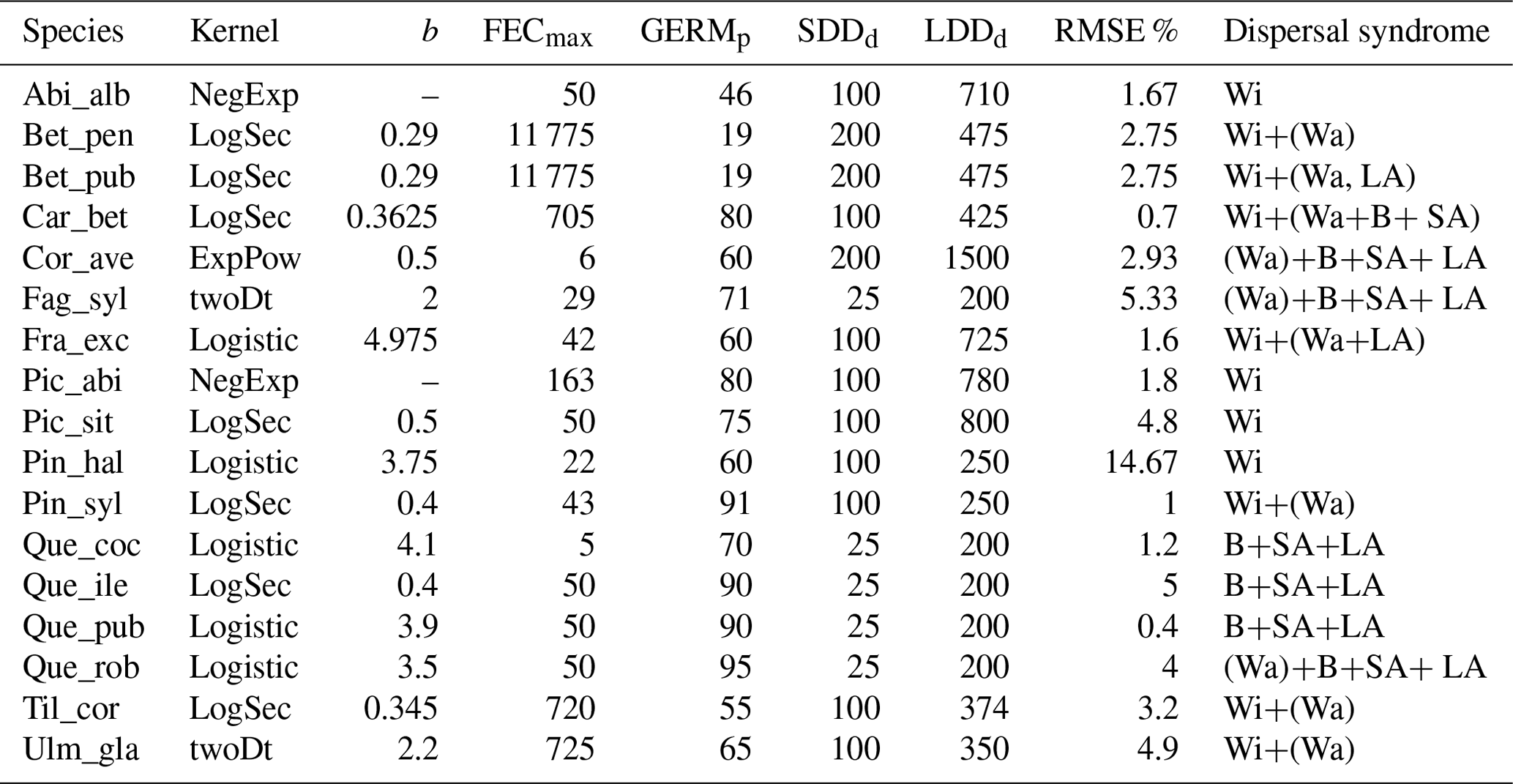
The model LPJ-GM 1.1 (LPJ-GUESS 4.0 coupled to a dynamic migration module) was used for the simulations presented in the study. The model code is archived in a private repository (https://github.com/zanid90/LPJ-GMINT, Zani and Lehsten, 2022), along with detailed instructions on how to compile and run the model version presented in this paper, where the model version is identified by the permanent version number v2.0-gm in the code repository. Access to the code is available upon request under license due to university policy (Lund University). Documentation and code base of the main version of LPJ-GUESS is available upon request under license via the LPJ-GUESS home page: https://web.nateko.lu.se/lpj-guess/ (Smith et al., 2021). An open-access educational version of the base code LPJ-GUESS is also available there. Input climate and landscape data filtered for the simulation domain, grid list, and instruction file with parameter settings for the LPJ-GM simulations are available at https://doi.org/10.18161/20211127 (Zani, 2021). Full climate and landscape data were provided by Armstrong et al. (2019).
The Supplement contains (1) the post-processing MATLAB script for the calculation of migration speed from the LPJ-GM output (post_processing/Postprocessing_plotMigrationRate.m with a sample output lai.out); (2) the .csv tables with migration speed separated by analysis (Input_SA.csv and Input_SA_model2.csv for the Sensitivity Analysis of the default and improved model structure, Sect. 2.5.1 and 2.6.2, respectively; Input_EVA.csv for the extreme value analysis, Sect. 2.5.2; Input_KA.csv for the kernel analysis, Sect. 2.6.1); (3) the Jupyter Notebook used to generate all figures and tables from the .csv data and statistical analyses performed in the study, including detailed information on the setting and parameters used in the LPJ-GM simulations (Supplement_Information.ipynb and Supplement_Information.pdf); and (4) supplementary tables (Table S1–3) and (5) figures (Fig. S1–4 in Supplement_Figures.pdf). The supplement related to this article is available online at: https://doi.org/10.5194/gmd-15-4913-2022-supplement.
DZ and VL designed the study, DZ performed the simulations and the statistical analysis, VL provided support with the coding, and VL and HL provided statistical support. All authors contributed to the writing of the paper.
The contact author has declared that neither they nor their co-authors have any competing interests.
Publisher's note: Copernicus Publications remains neutral with regard to jurisdictional claims in published maps and institutional affiliations.
This research has been supported by the Schweizerischer Nationalfonds zur Förderung der Wissenschaftlichen Forschung (grant no. Project “EXTRAS” 205320M_182609).
This paper was edited by Hisashi Sato and reviewed by two anonymous referees.
Albrich, K., Rammer, W., and Seidl, R.: Climate change causes critical transitions and irreversible alterations of mountain forests, Glob. Change Biol., 26, 4013–4027, https://doi.org/10.1111/gcb.15118, 2020.
Alexander, J. M., Chalmandrier, L., Lenoir, J., Burgess, T. I., Essl, F., Haider, S., Kueffer, C., McDougall, K., Nuñez, M. A., Pauchard, A., Rabitsch, W., Rew, L. J., Sanders, N. J., and Pellissier, L.: Lags in the response of mountain plant communities to climate change, Glob. Change Biol., 24, 563–579, https://doi.org/10.1111/gcb.13976, 2018.
Armstrong, E., Hopcroft, P. O., and Valdes, P. J.: A simulated Northern Hemisphere terrestrial climate dataset for the past 60,000 years, Sci Data, 6, 1–16, https://doi.org/10.1038/s41597-019-0277-1, 2019.
Baskin, C. C. and Baskin, J. M. Seeds: ecology, biogeography, and, evolution of dormancy and germination, Elsevier, https://doi.org/10.1016/B978-0-12-080260-9.X5000-3, 1998.
Beckman, N. G., Aslan, C. E., Rogers, H. S., Kogan, O., Bronstein, J. L., Bullock, J. M., Hartig, F., HilleRisLambers, J., Zhou, Y., Zurell, D., Brodie, J. F., Bruna, E. M., Cantrell, R. S., Decker, R. R., Efiom, E., Fricke, E. C., Gurski, K., Hastings, A., Johnson, J. S., Loiselle, B. A., Miriti, M. N., Neubert, M. G., Pejchar, L., Poulsen, J. R., Pufal, G., Razafindratsima, O. H., Sandor, M. E., Shea, K., Schreiber, S., Schupp, E. W., Snell, R. S., Strickland, C., and Zambrano, J.: Advancing an interdisciplinary framework to study seed dispersal ecology, AoB Plants, 12, https://doi.org/10.1093/aobpla/plz048, 2020.
Bennett, K. D., Tzedakis, P. C., and Willis, K. J. Quaternary refugia of north European trees, J. Biogeogr., 103–115, https://doi.org/10.2307/2845248, 1991.
Berg, M. P., Kiers, E. T., Driessen, G., Van Der Heijden, M., Kooi, B. W., Kuenen, F., Liefting, M., Verhoef, H. A., and Ellers, J.: Adapt or disperse: understanding species persistence in a changing world, Glob. Change Biol., 16, 587–598, https://doi.org/10.1111/j.1365-2486.2009.02014.x, 2010.
Binney, H. A., Willis, K. J., Edwards, M. E., Bhagwat, S. A., Anderson, P. M., Andreev, A. A., Blaauw, M., Damblon, F., Haesaerts, P., Kienast, F., Kremenetski, K. V., Krivonogov, S. K., Lozhkin, A. V., MacDonald, G. M., Novenko, E. Y., Oksanen, P., Sapelko, T. V., Väliranta, M., and Vazhenina, L.: The distribution of late-Quaternary woody taxa in northern Eurasia: evidence from a new macrofossil database, Quaternary Sci. Rev., 28, 2445–2464, https://doi.org/10.1016/j.quascirev.2009.04.016, 2009.
Birks, H. J. B.: Contributions of Quaternary botany to modern ecology and biogeography, Plant Ecol. Divers., 12, 189–385, https://doi.org/10.1080/17550874.2019.1646831, 2019.
Birks, H. J. B. and Birks, H. H.: Biological responses to rapid climate change at the Younger Dryas–Holocene transition at Kråkenes, western Norway, Holocene, 18, 19–30, https://doi.org/10.1177/0959683607085572, 2008.
Briscoe, N. J., Elith, J., Salguero-Gómez, R., Lahoz-Monfort, J. J., Camac, J. S., Giljohann, K. M., Holde, M. H., Hradsky, B. A., Kearney, M. R., McMahon, S. M., Phillips, B. L., Regan, T. J., Rhodes, J. R., Vesk, P. A., Wintle, B. A., Yen, J. D. L., and Guillera-Arroita, G.: Forecasting species range dynamics with process-explicit models: matching methods to applications, Ecol. Lett., 22, 1940–1956, https://doi.org/10.1111/ele.13348, 2019.
Bugmann, H.: On the ecology of mountainous forests in a changing climate: a simulation study, Doctoral dissertation, ETH Zurich, https://doi.org/10.3929/ethz-a-00094650, 1994.
Bullock, J. M. and Clarke, R. T.: Long distance seed dispersal by wind: measuring and modelling the tail of the curve, Oecologia, 124, 506–521, https://doi.org/10.1007/PL00008876, 2000.
Bullock, J. M., Mallada González, L., Tamme, R., Götzenberger, L., White, S. M., Pärtel, M., and Hooftman, D. A.: A synthesis of empirical plant dispersal kernels, J. Ecol., 105, 6–19, https://doi.org/10.1111/1365-2745.12666, 2017.
Cain, M. L., Damman, H., and Muir, A.: Seed dispersal and the Holocene migration of woodland herbs, Ecol. Monogr, 68, 325–347, https://doi.org/10.1890/0012-9615(1998)068[0325:SDATHM]2.0.CO;2, 1998.
Caswell, H., Lensink, R., and Neubert, M. G.: Demography and dispersal: life table response experiments for invasion speed, Ecology, 84, 1968–1978, https://doi.org/10.1890/02-0100, 2003.
Cheaib, A., Badeau, V., Boe, J., Chuine, I., Delire, C., Dufrêne, E., François, C., Gritti, E. S., Legay, M., Pagé, C., Thuiller, W., Viovy, N., and Leadley, P.: Climate change impacts on tree ranges: model intercomparison facilitates understanding and quantification of uncertainty, Ecol. Lett., 15, 533–544, https://doi.org/10.1111/j.1461-0248.2012.01764.x, 2012.
Chećko, E., Jaroszewicz, B., Olejniczak, K., and Kwiatkowska-Falińska, A. J.: The importance of coarse woody debris for vascular plants in temperate mixed deciduous forests, Can. J. Forest Res., 45, 1154–1163, https://doi.org/10.1139/cjfr-2014-0473, 2015.
Clark, J. S.: Why trees migrate so fast: confronting theory with dispersal biology and the paleorecord, Am. Nat., 152, 204–224, https://doi.org/10.1086/286162, 1998.
Clark, J. S., Silman, M., Kern, R., Macklin, E., and HilleRisLambers, J.: Seed dispersal near and far: patterns across temperate and tropical forests, Ecology, 80, 1475–1494, https://doi.org/10.1890/0012-9658(1999)080[1475:SDNAFP]2.0.CO;2, 1999.
Clark, J. S., Lewis, M., and Horvath, L.: Invasion by extremes: population spread with variation in dispersal and reproduction, Am. Nat., 157, 537–554, https://doi.org/10.1086/319934, 2001.
Clark, J. S., Lewis, M., McLachlan, J. S., and HilleRisLambers, J. Estimating population spread: what can we forecast and how well?, Ecology, 84, 1979–1988, https://doi.org/10.1890/01-0618, 2003.
Collingham, Y. C. and Huntley, B. Impacts of habitat fragmentation and patch size upon migration rates, Ecol. Appl., 10, 131–144, https://doi.org/10.1890/1051-0761(2000)010[0131:IOHFAP]2.0.CO;2, 2000.
Corlett, R. T. and Westcott, D. A.: Will plant movements keep up with climate change?, Trends Ecol. Evol., 28, 482–488, https://doi.org/10.1016/j.tree.2013.04.003, 2013.
Cousens, R. D., Hughes, B. D., and Mesgaran, M. B.: Why we do not expect dispersal probability density functions based on a single mechanism to fit real seed shadows, J. Ecol., 106, 903–906, https://doi.org/10.1111/1365-2745.12891, 2018.
Daniell, J. R. G.: A dendrochronological study of subfossil Pinus sylvestris L. stumps from peat deposits at Badanloch in the far north of Scotland, Doctoral dissertation, Durham University, http://etheses.dur.ac.uk/6140/ (last access: 16 February 2022), 1992.
Daniell, J. R. G.: The Late-Holocene palaeoecology of Scots pine (Pinus sylvestris L.) in north-west Scotland, Doctoral dissertation, Durham University, http://etheses.dur.ac.uk/1219/ (last access: 16 February 2022), 1997.
De Meester, L., Stoks, R., and Brans, K. I. Genetic adaptation as a biological buffer against climate change: Potential and limitations, Integr. Zool., 13, 372–391, https://doi.org/10.1111/1749-4877.12298, 2018.
Downing, D. J., Gardner, R. H., and Hoffman, F. O.: An examination of response-surface methodologies for uncertainty analysis in assessment models, Technometrics, 27, 151–163, https://doi.org/10.1080/00401706.1985.10488032, 1985.
Dullinger, S., Dirnböck, T., and Grabherr, G.: Modelling climate change-driven treeline shifts: relative effects of temperature increase, dispersal and invasibility, J. Ecol., 92, 241–252, https://doi.org/10.1111/j.0022-0477.2004.00872.x, 2004.
Dullinger, S., Dendoncker, N., Gattringer, A., Leitner, M., Mang, T., Moser, D., Mücher, C. A., Plutzar, C., Mark Rounsevell, M., Willner, W., Zimmermann, N. E., and Hülber, K.: Modelling the effect of habitat fragmentation on climate-driven migration of European forest understorey plants, Divers. Distrib., 21, 1375–1387, https://doi.org/10.1111/ddi.12370, 2015.
Feurdean, A., Bhagwat, S. A., Willis, K. J., Birks, H. J. B., Lischke, H., and Hickler, T.: Tree migration-rates: narrowing the gap between inferred post-glacial rates and projected rates, PLoS One, 8, e71797, https://doi.org/10.1371/journal.pone.0071797, 2013.
Gear, A. J. and Huntley, B. Rapid changes in the range limits of Scots pine 4000 years ago, Science, 251, 544–547, https://doi.org/10.1126/science.251.4993.544, 1991.
Giannakos, P.: Frugivory and seed dispersal by carnivores in the Rhodopi mountains of northern Greece, Doctoral dissertation, Durham University, http://etheses.dur.ac.uk/4900/ (last access: 16 February 2022), 1997.
Giesecke, T. and Brewer, S.: Notes on the postglacial spread of abundant European tree taxa, Veg. Hist. Archaeobot., 27, 337–349, https://doi.org/10.1007/s00334-017-0640-0, 2018.
Giesecke, T., Brewer, S., Finsinger, W., Leydet, M., and Bradshaw, R. H.: Patterns and dynamics of European vegetation change over the last 15,000 years, J. Biogeogr., 44, 1441–1456, https://doi.org/10.1111/jbi.12974, 2017.
Goto, S., Shimatani, K., Yoshimaru, H., and Takahashi, Y.: Fat-tailed gene flow in the dioecious canopy tree species Fraxinus mandshurica var. japonica revealed by microsatellites, Mol. Ecol., 15, 2985–2996, https://doi.org/10.1111/j.1365-294X.2006.02976.x, 2006.
Guo, F., Lenoir, J., and Bonebrake, T. C.: Land-use change interacts with climate to determine elevational species redistribution, Nat. Commun., 9, 1–7, https://doi.org/10.1038/s41467-018-03786-9, 2018.
Hamby, D. M.: A comparison of sensitivity analysis techniques, Health Phys., 68, 195–204, 1995.
Higgins, S. I., Clark, J. S., Nathan, R., Hovestadt, T., Schurr, F., Fragoso, J. M. V., Aguiar, M. R., Ribbens, E., and Lavorel, S.: Forecasting plant migration rates: managing uncertainty for risk assessment, J. Ecol., 91, 341–347, https://doi.org/10.1046/j.1365-2745.2003.00781.x, 2003a.
Higgins, S. I., Nathan, R., and Cain, M. L.: Are long-distance dispersal events in plants usually caused by nonstandard means of dispersal?, Ecology, 84, 1945–1956, https://doi.org/10.1890/01-0616, 2003b.
Huntley, B.: Extreme temporal interpolation of sparse data is not a sufficient basis to substantiate a claim to have uncovered Pleistocene forest microrefugia, New Phytol., 204, 447–449, https://doi.org/10.1111/nph.12941, 2014.
Huntley, B. and Birks, H. J. B. (Eds.): Atlas of past and present pollen maps for Europe: 0–13,000 years ago, Cambridge University Press, https://doi.org/10.1017/S0079497X00007660, 1983.
Huntley, B., Daniell, J. R., and Allen, J. R. Scottish vegetation history: the Highlands, Bot. J. Scot., 49, 163–175, https://doi.org/10.1080/03746609708684864, 1997.
Huntley, B., Allen, J. R., Collingham, Y. C., Hickler, T., Lister, A. M., Singarayer, J., Stuart, A. J., Sykes, M. T., and Valdes, P. J.: Millennial climatic fluctuations are key to the structure of last glacial ecosystems, PLoS One, 8, e61963, https://doi.org/10.1371/journal.pone.0061963, 2013.
Kattge, J., Bönisch, G., Díaz, S., Lavorel, S., Prentice, I. C., Leadley, P., et al.: TRY plant trait database–enhanced coverage and open access, Glob Change Biol., 26, 119–188, https://doi.org/10.1111/gcb.14904, 2020.
Klein, E. K., Lavigne, C., Picault, H., Renard, M., and Gouyon, P. H.: Pollen dispersal of oilseed rape: estimation of the dispersal function and effects of field dimension, J. Appl. Ecol., 43, 141–151, https://doi.org/10.1111/j.1365-2664.2005.01108.x, 2006.
Lehsten, V., Mischurow, M., Lindström, E., Lehsten, D., and Lischke, H.: LPJ-GM 1.0: simulating migration efficiently in a dynamic vegetation model, Geosci. Model Dev., 12, 893–908, https://doi.org/10.5194/gmd-12-893-2019, 2019.
Lenoir, J., Bertrand, R., Comte, L., Bourgeaud, L., Hattab, T., Murienne, J., and Grenouillet, G.: Species better track climate warming in the oceans than on land, Nature Ecol. Evol., 4, 1044–1059, https://doi.org/10.1038/s41559-020-1198-2, 2020.
Lischke, H. and Löffler, T. J.: Intra-specific density dependence is required to maintain species diversity in spatio-temporal forest simulations with reproduction, Ecol. Model., 198, 341–361, https://doi.org/10.1016/j.ecolmodel.2006.05.005, 2006.
Lischke, H., Zimmermann, N. E., Bolliger, J., Rickebusch, S., and Löffler, T. J.: TreeMig: a forest-landscape model for simulating spatio-temporal patterns from stand to landscape scale, Ecol. Model., 199, 409–420, https://doi.org/10.1016/j.ecolmodel.2005.11.046, 2006.
Lovas-Kiss, Á., Vizi, B., Vincze, O., Molnár V., A., and Green, A. J.: Endozoochory of aquatic ferns and angiosperms by mallards in Central Europe, J. Ecol., 106, 1714–1723, https://doi.org/10.1111/1365-2745.12913, 2018.
Lustenhouwer, N., Moran, E. V., and Levine, J. M.: Trait correlations equalize spread velocity across plant life histories, Global Ecol. Biogeogr., 26, 1398–1407, https://doi.org/10.1111/geb.12662, 2017.
Loehle, C.: Challenges of ecological complexity, Ecol. Complex., 1, 3–6, https://doi.org/10.1016/j.ecocom.2003.09.001, 2004.
Manel, S., Gaggiotti, O. E., and Waples, R. S.: Assignment methods: matching biological questions with appropriate techniques, Trends Ecol. Evol., 20, 136–142, https://doi.org/10.1016/j.tree.2004.12.004, 2005.
MacDonald, G. M.: Fossil pollen analysis and the reconstruction of plant invasions, Adv. Ecol. Res., 24, 67–110, https://doi.org/10.1016/S0065-2504(08)60041-0, 1993.
McKenzie, P. F., Duveneck, M. J., Morreale, L. L., and Thompson, J. R.: Local and global parameter sensitivity within an ecophysiologically based forest landscape model, Environ. Modell. Softw., 117, 1–13, https://doi.org/10.1016/j.envsoft.2019.03.002, 2019.
Mersmann, O., Bischl, B., Trautmann, H., Preuss, M., Weihs, C., and Rudolph, G.: Exploratory landscape analysis, in: Proceedings of the 13th annual conference on Genetic and evolutionary computation, GECCO '11: Genetic and Evolutionary Computation Conference, Dublin, Ireland, 12–16 July 2011, 829–836, https://doi.org/10.1145/2001576.2001690, July, 2011.
Mladenoff, D. J.: LANDIS and forest landscape models, Ecol. Modell., 180, 7–19, https://doi.org/10.1016/j.ecolmodel.2004.03.016, 2004.
Morales, P., Hickler, T., Rowell, D. P., Smith, B., and Sykes, M. T.: Changes in European ecosystem productivity and carbon balance driven by regional climate model output, Glob. Change Biol., 13, 108–122, https://doi.org/10.1111/j.1365-2486.2006.01289.x, 2007.
Moran, E. V. and Clark, J. S.: Estimating seed and pollen movement in a monoecious plant: a hierarchical Bayesian approach integrating genetic and ecological data, Mol. Ecol., 20, 1248–1262, https://doi.org/10.1111/j.1365-294X.2011.05019.x, 2011.
Nathan, R. and Katul, G. G.: Foliage shedding in deciduous forests lifts up long-distance seed dispersal by wind, P. Natl. Aacad. Sci. USA, 102, 8251–8256, https://doi.org/10.1073/pnas.0503048102, 2005.
Nathan, R., Schurr, F. M., Spiegel, O., Steinitz, O., Trakhtenbrot, A., and Tsoar, A.: Mechanisms of long-distance seed dispersal, Trends Ecol. Evol., 23, 638–647, https://doi.org/10.1016/j.tree.2008.08.003, 2008.
Nathan, R., Klein, E. K., Robledo-Arnuncio, J. J., and Revilla, E.: Dispersal kernels: review, in: Dispersal Ecology and Evolution, Oxford Scholarship Online, 187–210, https://doi.org/10.1093/acprof:oso/9780199608898.001.0001, 2012.
Nobis, M. P. and Normand, S.: KISSMig – a simple model for R to account for limited migration in analyses of species distributions, Ecography, 37, 1282–1287, https://doi.org/10.1111/ecog.00930, 2014.
Normand, S., Ricklefs, R. E., Skov, F., Bladt, J., Tackenberg, O., and Svenning, J. C.: Postglacial migration supplements climate in determining plant species ranges in Europe, P. Roy. Soc. B-Biol. Sci., 278, 3644–3653, https://doi.org/10.1098/rspb.2010.2769, 2011.
Nogués-Bravo, D., Rodríguez-Sánchez, F., Orsini, L., de Boer, E., Jansson, R., Morlon, H., Fordham, D. A., and Jackson, S. T.: Cracking the code of biodiversity responses to past climate change, Trends Ecol. Evol., 33, 765–77, https://doi.org/10.1016/j.tree.2018.07.005, 2018.
Palmé, A. E., Su, Q., Rautenberg, A., Manni, F., and Lascoux, M.: Postglacial recolonization and cpDNA variation of silver birch, Betula pendula, Mol. Ecol., 12, 201–212, https://doi.org/10.1046/j.1365-294X.2003.01724.x, 2003.
Pappas, C., Fatichi, S., Leuzinger, S., Wolf, A., and Burlando, P.: Sensitivity analysis of a process-based ecosystem model: Pinpointing parameterization and structural issues, J. Geophys. Res.-Biogeo., 118, 505–528, https://doi.org/10.1002/jgrg.20035, 2013.
Pecl, G. T., Araújo, M. B., Bell, J. D., Blanchard, J., Bonebrake, T. C., Chen, I. C., Clark, T. D., Colwel, R. K., Danielsen, F., Evengård, B., Falconi, L., Ferrier, S., Frusher, S., Garcia, R. A., Griffis, R. B., Hobday, A. J., Janion-Scheepers, C., Jarzyna, M. A., Jennings, S., Lenoir, J., Linnetved, H. I., Martin, V. Y., McCormack, P. C., McDonald, J., Mitchell, N. J., Mustonen, T., Pandolfi, J. M., Pettorelli, N., Popova, E., Robinson, S. A., Scheffers, B. R., Shaw, J. D., Sorte, C. J. B., Strugnell, J. M., Sunday, J. M., Tuanmu, M.-N., Vergés, A., Villanueva, C., Wernberg, T., Wapstra, E., and Williams, S. E.: Biodiversity redistribution under climate change: Impacts on ecosystems and human well-being, Science, 355, eaai9214, https://doi.org/10.1126/science.aai9214, 2017.
Petit, R. J., Brewer, S., Bordács, S., Burg, K., Cheddadi, R., Coart, E., Cottrell, J., Csaikl, U. M., van Dam, B., Deans, J. D., Espinel, S., Fineschi, S., Finkeldey, R., Glaz, I., Goicoechea, P. G., Jensen, J. S., König, A. O., Lowe, A. J., Madsen, S. F., Mátyás, G., Munro, R. C., Popescu, F., Slade, D., Tabbener J., de Vries, S. G. M., Ziegenhagen, B., de Beaulieu J.-L., and Kremer, A.: Identification of refugia and post-glacial colonisation routes of European white oaks based on chloroplast DNA and fossil pollen evidence, Forest Ecol. Manag., 156, 49–74, https://doi.org/10.1016/S0378-1127(01)00634-X, 2002.
Petter, G., Mairota, P., Albrich, K., Bebi, P., Brůna, J., Bugmann, H., Haffenden, A., Scheller, R. M., Schmatz, D. R., Seidl, R., Speich, M., Vacchiano, G., and Lischke, H.: How robust are future projections of forest landscape dynamics? Insights from a systematic comparison of four forest landscape models, Environ. Modell. Softw., 134, 104844, https://doi.org/10.1016/j.envsoft.2020.104844, 2020.
Powell, J. A. and Zimmermann, N. E.: Multiscale analysis of active seed dispersal contributes to resolving Reid's paradox, Ecology, 85, 490–506, https://doi.org/10.1890/02-0535, 2004.
Reid, C.: The origin of the British flora, Dulau, London, https://doi.org/10.1038/062268a0, 1899.
Rogers, H. S., Beckman, N. G., Hartig, F., Johnson, J. S., Pufal, G., Shea, K., Zurell, D., Bullock, J. M., Cantrell, R. S., Loiselle, B., Pejchar, L., Razafindratsima, O. H., Sandor, M. E., Schupp, E. W., Strickland, W. C., and Zambrano, J.: The total dispersal kernel: a review and future directions, AoB Plants, 11, https://doi.org/10.1093/aobpla/plz042, 2019.
Royal Botanic Gardens Kew: Seed Information Database (SID), Version 7.0., http://data.kew.org/sid/, last access: 19 December 2019.
Saltelli, A., Tarantola, S., and Campolongo, F.: Sensitivity analysis as an ingredient of modeling, Stat. Sci., 15, 377–395, https://doi.org/10.1214/ss/1009213004, 2000.
Saltré, F., Duputié, A., Gaucherel, C., and Chuine, I.: How climate, migration ability and habitat fragmentation affect the projected future distribution of European beech, Glob. Change Biol., 21, 897–910, https://doi.org/10.1111/gcb.12771, 2015.
Scherrer, D., Vitasse, Y., Guisan, A., Wohlgemuth, T., and Lischke, H.: Competition and demography rather than dispersal limitation slow down upward shifts of trees' upper elevation limits in the Alps, J. Ecol., 108, 2416–2430, https://doi.org/10.1111/1365-2745.13451, 2020.
Schumacher, S., Bugmann, H., and Mladenoff, D. J.: Improving the formulation of tree growth and succession in a spatially explicit landscape model, Ecol. Modell., 180, 175–194, https://doi.org/10.1016/j.ecolmodel.2003.12.055, 2004.
Schurr, F. M., Spiegel, O., Steinitz, O., Trakhtenbrot, A., Tsoar, A., and Nathan, R.: Long-distance seed dispersal, in: Annual Plant Reviews, Fruit Development and Seed Dispersal, edited by: Østergaard, L., Blackwell Publishing Ltd., 38, 204–237, https://doi.org/10.1002/9781444314557.ch6, 2009.
Seidl, R., Rammer, W., Scheller, R. M., and Spies, T. A.: An individual-based process model to simulate landscape-scale forest ecosystem dynamics, Ecol. Modell., 231, 87–100, https://doi.org/10.1016/j.ecolmodel.2012.02.015, 2012.
Shifley, S. R., He, H. S., Lischke, H., Wang, W. J., Jin, W., Gustafson, E. J., Thompson, J. R., Thompson, F. R., Dijak,W. D., and Yang, J.: The past and future of modeling forest dynamics: from growth and yield curves to forest landscape models, Landscape Ecol., 32, 1307–1325, https://doi.org/10.1007/s10980-017-0540-9, 2017.
Smith, B., Prentice, I. C., and Sykes, M. T.: Representation of vegetation dynamics in the modelling of terrestrial ecosystems: comparing two contrasting approaches within European climate space, Global Ecol. Biogeogr., 10, 621–637, 2001.
Smith, B., Arneth, A., Arvanitis, T., Bondeau, A., Chaudhary, N., Cramer, W., Eliasson, P., Gerten, D., Hickler, T., Holmér, J., Kaplan, J., Knorr, W., Lehsten, D., Lehsten, V., Lindeskog, M., Lucht, W., Miller, P., Mishurov, M., Olin, S., Poska, A., Pugh, T., Prentice, C., Rammig, A., Schaphoff, S., Schurgers, G., Siltberg, J., Sitch, S., Sykes, M., Thonicke, K., Venevsky, S., Wania, R., Wårlind, D., Wolf, A., Wramneby, A., and Zaehle, S.: LPJ-GUESS Education 3.0, https://web.nateko.lu.se/lpj-guess/, last access: 28 October 2021.
Snell, R. S., Huth, A., Nabel, J. E., Bocedi, G., Travis, J. M., Gravel, D., Bugmann, H., Gutiérrez, A. G., Hickler, T., Higgins, S. I., Reineking, B., Scherstjanoi, M., Zurbriggen, N., and Lischke, H.: Using dynamic vegetation models to simulate plant range shifts, Ecography, 37, 1184–1197, https://doi.org/10.1111/ecog.00580, 2014.
Soons, M. B., Heil, G. W., Nathan, R., and Katul, G. G.: Determinants of long-distance seed dispersal by wind in grasslands, Ecology, 85, 3056–3068, https://doi.org/10.1890/03-0522, 2004.
Snowling, S. D. and Kramer, J. R.: Evaluating modelling uncertainty for model selection, Ecol. Modell., 138, 17–30, https://doi.org/10.1016/S0304-3800(00)00390-2, 2001.
Stewart, J. R. and Lister, A. M.: Cryptic northern refugia and the origins of the modern biota, Trends Ecol. Evol., 16, 608–613, https://doi.org/10.1016/S0169-5347(01)02338-2, 2001.
Stork, J., Eiben, A. E., and Bartz-Beielstein, T.: A new taxonomy of global optimization algorithms, Nat. Comput., 21, 219–242, https://doi.org/10.1007/s11047-020-09820-4, 2020.
Svenning, J. C. and Sandel, B.: Disequilibrium vegetation dynamics under future climate change, Am. J. Bot., 100, 1266–1286, https://doi.org/10.3732/ajb.1200469, 2013.
Tamme, R., Götzenberger, L., Zobel, M., Bullock, J. M., Hooftman, D. A., Kaasik, A., and Pärtel, M.: Predicting species' maximum dispersal distances from simple plant traits, Ecology, 95, 505–513, https://doi.org/10.1890/13-1000.1, 2014.
Thompson, P. L. and Fronhofer, E. A.: The conflict between adaptation and dispersal for maintaining biodiversity in changing environments, P. Natl. Aacad. Sci. USA, 116, 21061–21067, https://doi.org/10.1073/pnas.1911796116, 2019.
Tomiolo, S. and Ward, D.: Species migrations and range shifts: A synthesis of causes and consequences, Perspect. Plant Ecol., 33, 62–77, https://doi.org/10.1016/j.ppees.2018.06.001, 2018.
Tzedakis, P. C., Emerson, B. C., and Hewitt, G. M.: Cryptic or mystic? Glacial tree refugia in northern Europe, Trends Ecol. Evol., 28, 696–704, https://doi.org/10.1016/j.tree.2013.09.001, 2013.
Vittoz, P. and Engler, R.: Seed dispersal distances: a typology based on dispersal modes and plant traits, Bot. Helv., 117, 109–124, https://doi.org/10.1007/s00035-007-0797-8, 2007.
Wilkinson, D. M.: Plant colonization: are wind dispersed seeds really dispersed by birds at larger spatial and temporal scales?, J. Biogeogr., 24, 61–65, https://doi.org/10.1111/j.1365-2699.1997.tb00050.x, 1997.
Wilson, G. A. and Rannala, B.: Bayesian inference of recent migration rates using multilocus genotypes, Genetics, 163, 1177–1191, https://doi.org/10.1093/genetics/163.3.1177, 2003.
Wramneby, A., Smith, B., Zaehle, S., and Sykes, M. T.: Parameter uncertainties in the modelling of vegetation dynamics–effects on tree community structure and ecosystem functioning in European forest biomes, Ecol. Model., 216, 277–290, https://doi.org/10.1016/j.ecolmodel.2008.04.013, 2008.
Zaehle, S., Sitch, S., Smith, B., and Hatterman, F.: Effects of parameter uncertainties on the modeling of terrestrial biosphere dynamics, Global Biogeochem. Cy., 19, https://doi.org/10.1029/2004GB002395, 2005.
Zani, D.: Input climate and landscape data to “Tree migration in the dynamic, global vegetation model LPJ-GM 1.1”, DatGURU [data set], https://doi.org/10.18161/20211127, 2021.
Zani, D. and Lehsten, V.: LPJ-GMINT, Dynamic vegetation model (LPJ-Guess) with migration (M) and interacting non-tree species (INT) modules, GitHub [code], https://github.com/zanid90/LPJ-GMINT (last access: 1 November 2021), 2022.
- Abstract
- Introduction
- Material and methods
- Results
- Discussion
- Limitations and future challenges
- Conclusions
- Appendix A: Migration module of the model LPJ-GM 1.0
- Appendix B: Migration parameters
- Code and data availability
- Author contributions
- Competing interests
- Disclaimer
- Financial support
- Review statement
- References
- Supplement