the Creative Commons Attribution 4.0 License.
the Creative Commons Attribution 4.0 License.
 | 27 Jun 2022
Description and evaluation of the tropospheric aerosol scheme in the Integrated Forecasting System (IFS-AER, cycle 47R1) of ECMWF
Zak Kipling
Vincent Huijnen
Johannes Flemming
Pierre Nabat
Martine Michou
Melanie Ades
Richard Engelen
Vincent-Henri Peuch
This article describes the Integrated Forecasting System aerosol scheme (IFS-AER) used operationally in the IFS cycle 47R1, which was operated by the European Centre for Medium Range Weather Forecasts (ECMWF) in the framework of the Copernicus Atmospheric Monitoring Services (CAMS). It represents an update of the Rémy et al. (2019) article, which described cycle 45R1 of IFS-AER in detail. Here, we detail only the parameterisations of sources and sinks that have been updated since cycle 45R1, as well as recent changes in the configuration used operationally within CAMS. Compared to cycle 45R1, a greater integration of aerosol and chemistry has been achieved. Primary aerosol sources have been updated, with the implementation of new dust and sea salt aerosol emission schemes. New dry and wet deposition parameterisations have also been implemented. Sulfate production rates are now provided by the global chemistry component of IFS. This paper aims to describe most of the updates that have been implemented since cycle 45R1, not just the ones that are used operationally in cycle 47R1; components that are not used operationally will be clearly flagged.
Cycle 47R1 of IFS-AER has been evaluated against a wide range of surface and total column observations. The final simulated products, such as particulate matter (PM) and aerosol optical depth (AOD), generally show a significant improvement in skill scores compared to results obtained with cycle 45R1. Similarly, the simulated surface concentration of sulfate, organic matter and sea salt aerosol are improved by cycle 47R1 compared to cycle 45R1. Some biases persist, such as the surface concentrations of nitrate and organic matter being simulated too high. The new wet and dry deposition schemes that have been implemented into cycle 47R1 have a mostly positive impact on simulated AOD, PM and speciated aerosol surface concentration.
- Article
(4397 KB) - Full-text XML
- BibTeX
- EndNote


The Copernicus Atmosphere Monitoring Service (CAMS), operated by the European Centre for Medium Range Weather Forecasts (ECMWF) on behalf of the European Commission, has provided operationally near-real-time global analyses and 5 d forecasts of aerosol, trace gases and greenhouse gases twice daily since 2014. It also released the CAMS reanalysis of atmospheric composition (Inness et al., 2019) in September 2018, which has been continually updated since then and now covers 2003 to 2020. These global analyses and forecasts are provided by ECMWF's Integrated Forecasting System (IFS), which combines state-of-the-art meteorological and atmospheric composition modelling together with the data assimilation of satellite products. IFS, with its atmospheric composition extensions, was first developed in the framework of the Global and regional Earth system Monitoring using Satellite and in situ data project (GEMS; 2005 to 2009; Hollingsworth et al., 2008), followed by the Monitoring Atmospheric Composition and Climate series of projects (MACC, MACC-II and MACC-III; 2010 to 2014), and finally CAMS (2014 to present). IFS is originally a numerical weather prediction system dedicated to operational meteorological forecasts. It was extended to forecast and assimilate aerosols (Morcrette et al., 2009; Benedetti et al., 2009; Rémy et al., 2019), greenhouse gases (Engelen et al., 2009; Agustí-Panareda et al., 2014), tropospheric reactive trace gases (Flemming et al., 2009, 2015; Huijnen et al., 2016) and stratospheric reactive gases (Huijnen et al., 2016). “IFS-AER” denotes IFS extended with the bin and bulk aerosol scheme used to provide global aerosol products in the CAMS project.
The parameterisations of IFS-AER cycle 38R2 and cycle 45R1 have been extensively described in Morcrette et al. (2009) and Rémy et al. (2019), respectively. Here, we aim to describe the updates of IFS-AER that have been implemented since cycle 45R1. Most of these updates are used in the version of cycle 47R1 used for operational forecasts, with the exception of the new dry and wet deposition schemes, which were not used operationally in cycle 47R1 for technical reasons but are now used in operational cycle CY47R3. A total of 1 year of cycling forecasts with 45R1 and 47R1 IFS-AER have been evaluated against an extensive set of ground and remote sensing observational datasets. “Cycling forecasts” refer to experiments that use data assimilation for the meteorological initial conditions but not for the aerosol and chemical tracers; 24 h forecasts from the previous cycle are used as initial conditions for these tracers.
In Sect. 2 we present the main characteristics of IFS-AER, and its coupling to the operational global chemistry scheme IFS-CB05 is described. Section 3 details the current and past operational configurations. Section 4 details the changes since cycle 45R1 in the representation of primary aerosol sources. Section 5 presents the upgrade of the aerosol wet and dry deposition. Finally, Sect. 6 presents simulation results and budgets and a global and regional evaluation of cycle 45R1 and 47R1 IFS-AER simulations against remote sensing products and ground observations.
Table 1Aerosol species and parameters of the number size distribution associated to each aerosol type in IFS-AER (rmod is mode radius, ρ is particle density and σ is geometric standard deviation). Values are for the dry aerosol, with the exception of sea salt, which is given at 80 % RH. The number size distribution is assumed to be monomodal for all species except sea salt and coarse-mode nitrate for which a bimodal size distribution is assumed.

IFS-AER is a bulk aerosol scheme with three bins for all species (except sea salt aerosol and desert dust, for which a sectional approach is preferred). As such, it is often denoted as a “bulk–bin” scheme; IFS-AER derives from the Laboratoire d'Optique Atmosphérique/Laboratoire de Météorologie Dynamique - Zoom (LOA/LMDZ) model (Boucher et al., 2002; Reddy et al., 2005) and uses a mass mixing ratio as the prognostic variable of the aerosol tracers. The aerosol species and the assumed number size distribution are shown in Table 1. In contrast to Rémy et al. (2019), only the nitrate and ammonium species differ. Since the implementation of operational cycle 46R1 in July 2019, the prognostic species are sea salt, desert dust, organic matter (OM), black carbon (BC), sulfate, nitrate and ammonium. IFS-AER is by default run coupled with the operational Carbon Bond 2005 (CB05, Yarwood et al., 2005) tropospheric chemistry scheme that has been integrated into the IFS (Flemming et al., 2015) and is from here on referred to as “IFS-CB05”. IFS-AER can also be run in stand-alone mode, i.e. without any interaction with the chemistry, in which case the nitrate and ammonium species are not included and a specific tracer representing sulfur dioxide is added, as described in Rémy et al. (2019).
Desert dust is represented with three size bins, with radius bin limits at 0.03, 0.55, 0.9 and 20 µm). Sea salt aerosol is also represented with three size bins, with radius bin limits of 0.03, 0.5, 5 and 20 µm at 80 % relative humidity. All of the sea salt aerosol parameters (concentration, emission, deposition) are expressed at 80 % relative humidity; this is in contrast to the other aerosol species in IFS-AER, which are expressed as dry mixing ratio. The sea salt aerosol mass mixing ratio, as well as the emissions, burden and sink diagnostics, need to be divided by a factor of 4.3 to convert to dry mass mixing ratio in order to account for the hygroscopic growth and change in particle density. There is no mass transfer between bins for either dust or sea salt.
The organic matter and black carbon species consist of their hydrophilic and hydrophobic fractions, with the ageing processes transferring mass from the hydrophobic to hydrophilic components. Sulfate aerosols (and when not fully coupled to IFS-CB05, the precursor gas sulfur dioxide) are represented by one prognostic variable each. When running fully coupled with IFS-CB05, which has been the operational configuration since cycle 46R1, sulfur dioxide is represented in CB05 and thus not in IFS-AER. Since cycle 46R1, two extra species, nitrate and ammonium, have been included in the operational products. The nitrate species consists of two prognostic variables that represent fine nitrate produced by gas–particle partitioning and coarse nitrate produced by heterogeneous reactions of dust and sea salt particles. In all, IFS-AER is thus composed of 12 prognostic variables when running stand-alone and 14 when fully coupled with IFS-CB05 (including nitrates and ammonium), which allows for a relatively limited consumption of computing resources.
2.1 Coupling to the chemistry
One of the most important features of cycle 47R1 IFS-AER is its increasing integration of aerosol and chemistry. The sulfur and nitrogen cycles are now represented across IFS-AER (for particulate species) and IFS-CB05 (for gaseous species), and IFS-AER provides supplementary input to IFS-CB05 in order to better represent heterogeneous reactions and the impact of aerosols and photolysis rates.
2.1.1 Sulfur cycle
The simplistic representation of the conversion of sulfur dioxide into sulfate aerosol used operationally in cycle 45R1 IFS-AER (Rémy et al., 2019) has been replaced by a full coupling to the chemistry, through which the sulfate production rates are computed and provided by IFS-CB05. The sulfur chemistry in IFS-CB05 is as described in Huijnen et al. (2010). In short, in total 111 Tg SO2 is emitted, which is composed of 97 Tg anthropogenic emissions, 13 Tg volcanic emissions and 1 Tg biomass burning emissions. In addition, 38 Tg dimethyl sulfide (DMS) emissions taken from climatological values are applied, which is then oxidised to form SO2 (37 Tg) and the rest (5.3 Tg) of the methyl sulfonic acid (MSA). This leads to an annual production of 124 Tg sulfate, both through gas-phase oxidation with OH and aqueous-phase oxidation including reactions with H2O2 and O3.
Table 2Global budget for 2017 (annual mean) of SO2 and SO2 as simulated by IFS-AER standalone and coupled with IFS-CB05 (fluxes are expressed in Tg S yr−1; burden is expressed in Tg S).
The coupling with IFS-CB05 impacts most aspects of the simulated sulfur cycle. Table 2 shows the budgets of sulfur dioxide and sulfate aerosols for standalone IFS-AER (CY45R1) and IFS-AER (CY45R1) coupled with IFS-CB05 (CY47R1). The sulfur dioxide sources are slightly different in the standalone configuration: emissions from MACCity (Granier et al., 2011) are used for the SO2 tracer included in standalone IFS-AER, while the more recent CAMS_GLOB_ANT (Granier et al., 2019) are used for the sulfur dioxide tracer of IFS-CB05 in the coupled configuration. The different sulfur dioxide emissions explain part of the difference between the budgets and surface concentration plots shown below. The wet deposition of sulfur dioxide is represented in IFS-CB05 and not in the standalone version of IFS-AER, which adds an important sink to the simulated sulfur dioxide. Finally, the chemical conversion rates are globally of the same order of magnitude, but with large regional and vertical differences, leading to a much longer simulated lifetime of sulfur dioxide with cycle 47R1. There are no direct sulfate emissions in IFS-AER.
As shown in Table 2, the global budget of sulfate aerosol differs relatively little between the standalone (CY45R1) and coupled (CY47R1) IFS-AER, taking into account the fact that a new wet deposition routine is available in CY47R1, which will be detailed in Sect. 5.
2.1.2 Nitrate and ammonium
The production scheme of nitrate and ammonium through gas–particle partitioning processes and of nitrate from heterogeneous reactions on dust and sea salt particles is detailed in Rémy et al. (2019) and has been adapted from Hauglustaine et al. (2014), which uses the Equilibrium Simplified Aerosol Model (EQSAM, Metzger et al., 2002) approach. These two parameterisations use meteorological parameters provided by IFS and the gaseous precursors (nitric acid and ammonia) as input. The concentrations of the gaseous precursors are provided by IFS-CB05 and are updated alongside those of the particulate products (nitrate and ammonium) following gas–particle partitioning and heterogeneous reaction processes. The gas–particle partitioning scheme estimates nitrate and ammonium production through the neutralisation of HNO3 using the NH3 remaining after neutralisation by sulfuric acid:
The formation of nitrate from heterogeneous reactions of HNO3 with calcite (a component of dust aerosol) and sea salt particles is accounted for through the following reactions:
Table 3The 2017 global budget of nitrate aerosol from gas–particle partitioning and heterogeneous reactions and of ammonium aerosol as simulated by IFS-AER CY47R1 (fluxes are expressed in Tg N yr−1; burden is expressed in Tg N). The median values from Bian et al. (2017) are indicated in parentheses when they are available and comparable.
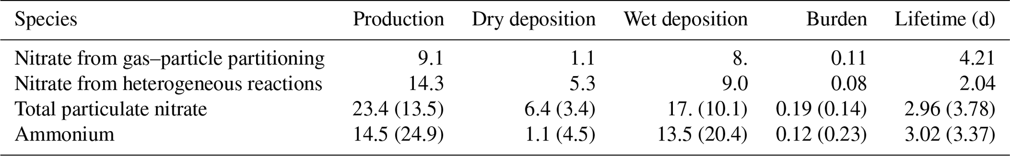
Table 3 shows the budget of the two nitrate species, total particulate nitrate and ammonium, compared with the median values from the AEROCOM phase III experiment (Bian et al., 2017). The comparison to values provided by Bian et al. (2017) can only be qualitative because the emission of the precursor gases (ammonia, nitrous oxides) are different, and the years simulated are also not the same. However, the fact that no major disagreement appears shows that values simulated by IFS-AER fall in the range of values simulated by other models.
2.2 Use of aerosol inputs in IFS-CB05
The global tropospheric chemistry module of IFS, IFS-CB05, uses aerosol mass mixing ratio input from IFS-AER to estimate the reaction rates of heterogeneous reactions on top of aerosol particles. The simulated absorption aerosol optical depth (AAOD) from IFS-AER also intervenes in the computation of photolysis rates Huijnen et al. (2016).
IFS-AER cycle 47R1 was used operationally to provide near-real-time (NRT) aerosol products within CAMS from October 2020 until May 2021, when the new cycle 47R2 became operational. The operational cycle 47R2 does not include any update to IFS-AER; the only feature that impacts simulated aerosol fields besides the upgrade of the meteorological model is the implementation of a maximum value on primary OM emissions, which is meant to compensate for the fact that the emission datasets used underestimate the recent decrease of emissions over China. More details on the implementation of cycle 47R2 can be found at https://confluence.ecmwf.int/display/COPSRV/Implementation+of+IFS+cycle+47r2 (last access: 13 January 2022). The operational cycle 47R2 also runs using single precision instead of double precision for previous operational cycles, which does not impact the output of chemistry and aerosol fields.
In the operational environment, cycle 47R1 IFS-AER assimilates aerosol optical depth (AOD) observations from MODIS collection 6.1 (Levy et al., 2013) and from the Polar Multi Angle Product (Popp et al., 2016). The horizontal and vertical resolution, as well as the time step, are unchanged compared to operational cycle 46R1, with TL511 (40 km grid cell), 137 levels over the vertical and 900 s. A definition of the vertical levels can be found at https://confluence.ecmwf.int/display/UDOC/L137+model+level+definitions, (last access: 20 January 2022). Prognostic aerosols are used as an input of the IFS radiation scheme to compute the direct radiative effect of aerosols.
Table 4IFS-AER cycles and options used operationally for near-real-time global CAMS products. MF stands for mass fixer, DDEP stands for dry deposition and SCON stands for sulfate conversion. G01 indicates the Ginoux et al. (2001) dust emission scheme, G01bis indicates the Ginoux et al. (2001) dust emission scheme with modified distribution of the emissions into the dust bins and N12 indicates the Nabat et al. (2012) dust emission scheme. M86, G14 and A16 indicate the Monahan et al. (1986), Grythe et al. (2014) and Albert et al. (2016) sea salt aerosol emission schemes, respectively. R05 corresponds to the version of the parameterisation described in Reddy et al. (2005). R05bis is the updated simple sulfate conversion scheme with temperature and relative humidity dependency. CF stands for the wet deposition parameterisation using condensation fluxes (as implemented in cycle 46R1). L19 stands for wet deposition based on Luo et al. (2019). ZH01 and ZH14 stand for the Zhang et al. (2001) and Zhang and He (2014) dry deposition parameterisations, respectively. MACCRA, CAMSiRA and CAMSRA are the MACC Reanalysis (Inness et al., 2013), the CAMS interim Reanalysis (Flemming et al., 2015) and the CAMS Reanalysis (Inness et al., 2019), respectively. For the three reanalyses, the date column refers to when the data were first publicly released.

Since cycle 46R1, injection heights provided by GFAS (Rémy et al., 2017) have been used for all aerosol and trace gas biomass burning emissions. Since cycle 43R1, as detailed in Rémy et al. (2019), direct anthropogenic SOA emissions scaled on anthropogenic CO emissions have been added to organic matter emissions. This large anthropogenic SOA source derives from the work of Spracklen et al. (2011), who found that they achieved best results in simulating secondary organic aerosols when they assumed a large SOA source (100 Tg per year) from sources that matched anthropogenic pollution. Biogenic SOA emissions that are taken as a 15 % fraction of natural terpene emissions following Dentener et al. (2006) are also added to organic matter emissions. A summary of the operational configurations of the latest versions of the NRT system during the CAMS and MACC projects, as well as the three reanalyses, is shown in Table 4. This table summarises the evolution of IFS-AER since 2013, as well as the changes in the emission datasets used and the horizontal and vertical resolution.
IFS uses a semi-implicit semi-Lagrangian (SL) advection scheme (Hortal, 2002). It is computationally efficient but does not conserve the tracer mass when the flow is convergent or divergent, which is often the case in the presence of orographic features. To compensate for this, mass fixers (MF) have been used for greenhouse gases (Agusti-Panareda et al., 2017), trace gases (Diamantakis and Flemming, 2014) and aerosols in IFS-AER since cycle 43R1.
The operational global CAMS products are routinely evaluated against a variety of observational datasets. The quarterly evaluation reports are available online and can be consulted at https://atmosphere.copernicus.eu/publications (last access: 10 June 2022).
This section describes the updates in the parameterisations of online aerosol emissions for dust and sea salt aerosol since cycle 45R1.
4.1 Sea salt aerosol
In addition to the M86 (Monahan et al., 1986) and the G14 (Grythe et al., 2014) sea salt aerosol emission schemes, a new sea salt emission scheme “A16” based on Albert et al. (2016) has been developed. It is similar to the M86 scheme in the sense that the oceanic whitecap fraction is first estimated as a prerequisite; in the M86 scheme this is done following the work of Monahan and Muircheartaigh (1980). In the A16 scheme, this is done using a statistical fit between a dataset of 1 year of whitecap fraction estimated from remote sensing observations of ocean surface brightness by radiometers onboard the WindSat satellite at two frequencies, i.e. 10 and 37 GHz (Anguelova and Webster, 2006), 10 m wind speed provided by QuickSCAT, and sea surface temperature (SST) provided by ERA-Interim. The whitecap fraction W is expressed as a function of 10 m wind speed U10 and SST by
where
The and b0,1 parameters are given in Albert et al. (2016) for the whitecap fraction estimated with WindSat 10 and 37 GHz brightness temperatures. As the coverage of the retrieved whitecap fraction dataset is very good, the sample size is very large, which makes the fit quite robust. In the IFS-AER implementation of this scheme, using the fit to whitecap from 37 GHz brightness temperature gave better results, and the and b0,1 parameters for this wavelength were chosen.
Using the oceanic whitecap fraction as an input, the production flux of sea salt aerosol is then computed by the following formula from Monahan et al. (1986):
where
and Dp is the particle diameter.
Table 5Dry sea salt aerosol emissions, burdens and lifetimes simulated by IFS-AER with the M86, G14 and A16 schemes (emissions are in Tg yr−1, burdens are in Tg and lifetimes are in d).
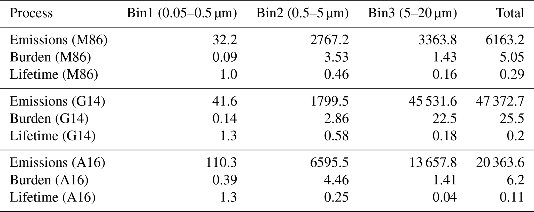
Table 5 shows the simulated emissions, burdens and lifetimes of the three sea salt bins for the three available emission schemes. The lifetime of sea salt aerosol decreases for larger particles because sedimentation, applied only to bin 3, is an effective sink and because the simulated dry deposition velocity increases with particle size for particles above 1 µm diameter. The emissions of super-coarse sea salt aerosol are much higher with the G14 scheme when compared to the two others. Similar to the M86 scheme, the A16 scheme shows a relatively small increase in emissions with bin size. The lifetime of coarse and super-coarse sea salt bins is the lowest with the A16 scheme. The M86 scheme was used operationally until cycle 43R3. The G14 scheme was used operationally in cycles 45R1 and 46R1, while the new A16 scheme was implemented in operational cycle CY47R1 of IFS-AER. More details about the A16 scheme can be found in Rémy and Anguelova (2021).
4.2 Desert dust
A new dust emission scheme has been implemented since cycle 46R1, which combines the approaches of Marticorena and Bergametti (1995) for the representation of the saltation process and of Kok (2011) for the size distribution of dust at emissions. This new dust scheme was adapted from the scheme implemented in TACTIC (Michou et al., 2015; Nabat et al., 2012).
The emissions of dust particles of a given size Dp through sandblasting occurs if the wind friction velocity u∗ is above a threshold value , which is written as follows:
where represents an ideal minimum threshold friction velocity and is determined according to the parameterisation of Marticorena and Bergametti (1995) as a function of the Reynolds number Re:
where the Reynolds number Re is parameterised following Marticorena and Bergametti (1995) as
and
where ρp is the dust aggregate density taken as 2.6 kg m−3, ρa is the surface air density and g the gravitational constant. The term feff is a correction factor accounting for the effect of surface roughness and is expressed as follows:
Finally, fw accounts for the effect of soil moisture content on the threshold friction velocity. Following Fecan et al. (1999), it is parameterised as follows:
where w is the surface soil moisture, provided by the IFS surface scheme, and
where %clay is the fraction of soil that is composed of clay. The information on the clay, silt and sand fraction is provided externally by the Global Soil Dataset for use in Earth system models (GSDE, Shangguan et al., 2014). The horizontal flux of dust from saltation is expressed as follows:
where Esoil is the soil “erodibility” and Srel is the ratio of the surface of the dust aggregate of diameter Dp over the sum of the surface of aggregates of all diameters. The soil erodibility can be defined as the soil erosion efficiency of a surface under a given meteorological forcing (Zender et al., 2003). It is also often denoted as “dust source function”. Because soil erodibility is hard to estimate, several methods have been tested in dust emission schemes, and one of the most commonly used is the topographic approach from Ginoux et al. (2001), which assumes that the topographic depressions are the largest source of dust. In the operational cycle 47R1, the soil erodibility is provided empirically by a climatological dataset of the frequency of occurrence of dust AOD > 0.4, as provided by Paul Ginoux and introduced in Ginoux et al. (2012). In cycle 46R1, the climatological frequency of dust AOD > 0.2 was used, which led to an overestimation of simulated dust AOD.
Table 6Desert dust emissions, burdens and lifetimes simulated by IFS-AER with the Ginoux01 (G01) and Nabat12 (N12) schemes (emissions are in Tg yr−1, burdens are in Tg and lifetimes are in d).

The friction velocity u∗ is computed using as an input the 10 m wind speed that includes a gustiness effect, computed as in Rémy et al. (2019). Finally, the flux of vertically emitted dust is computed from the horizontal flux using Gilette (1979):
where Fbare is the fraction of the soil that is bare; C is a normalisation constant set to 0.034, similar to the value used in Nabat et al. (2012) who used 0.035. This formula is integrated for all particle diameters Dp and provides the total flux of emitted dust. In order to distribute this flux into the three bins, the size distribution at emissions of Kok (2011) is used, which means a much larger share of emissions being distributed to the super-coarse bin compared to the Ginoux et al. (2001) scheme that was used operationally before cycle 46R1. This is illustrated by Table 6, and as a consequence the simulated lifetime of total dust is significantly lower with the new scheme compared to the old scheme because the super-coarse dust bin has a much shorter lifetime from increased dry deposition and sedimentation.
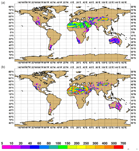
Figure 1Annual total emissions of dust for 2017 as simulated by CY45R1 and CY47R1 (b) (in ).
The 2017 annual total (sum of all bins) dust emissions with the two emission schemes is shown in Fig. 1. There is a much higher regional variability of yearly averaged dust emissions with the new scheme. In addition, dust emissions are higher in the Sahel and many parts of the Sahara and are mostly lower over the Taklamakan and Gobi deserts.
In this section, updates to the removal processes compared to the parameterisations implemented in cycle 45R1 of IFS-AER and described in Rémy et al. (2019) are presented.
5.1 Dry deposition
A new parameterisation of aerosol dry deposition following Zhang and He (2014) has been implemented in cycle 47R1 IFS-AER but is not used operationally for technical reasons and is expected to be used in CY47R3. The operational dry deposition scheme still follows the approach of Zhang et al. (2001), as adapted in Rémy et al. (2019). The Zhang and He (2014) has been implemented because it gave good results in a recent intercomparison of dry deposition schemes (Khan and Perlinger, 2017) and because it divides particles into size ranges, i.e. fine, coarse and giant (super-coarse), instead of using the particle size as an input. Only the surface resistance differs compared to the Zhang et al. (2001) scheme. The inverse of the surface resistance is also referred to as surface deposition velocity and denoted as Vs. It is computed as a function of the particle diameter Dp and friction velocity u∗ as follows:
where
where ai, bi, ci, di and ei are land-surface-dependent coefficients provided by Zhang and He (2014) and LAIMAX is the maximum leaf area index for a give land surface category. Figure 2 shows a comparison of the simulated dry deposition velocity of the two schemes over a particular land surface category (desert).

Figure 2Dry deposition velocity over a desertic surface, as a function of particle size, parameterised by the Zhang et al. (2001) and the Zhang and He (2014) schemes.
5.2 Wet deposition
5.2.1 In-cloud scavenging in cycle 46R1
Several updates have been added to the representation of in-cloud scavenging in cycle 46R1. The in-cloud scavenging rate (in s−1) at model level k of an aerosol i is written as follows:
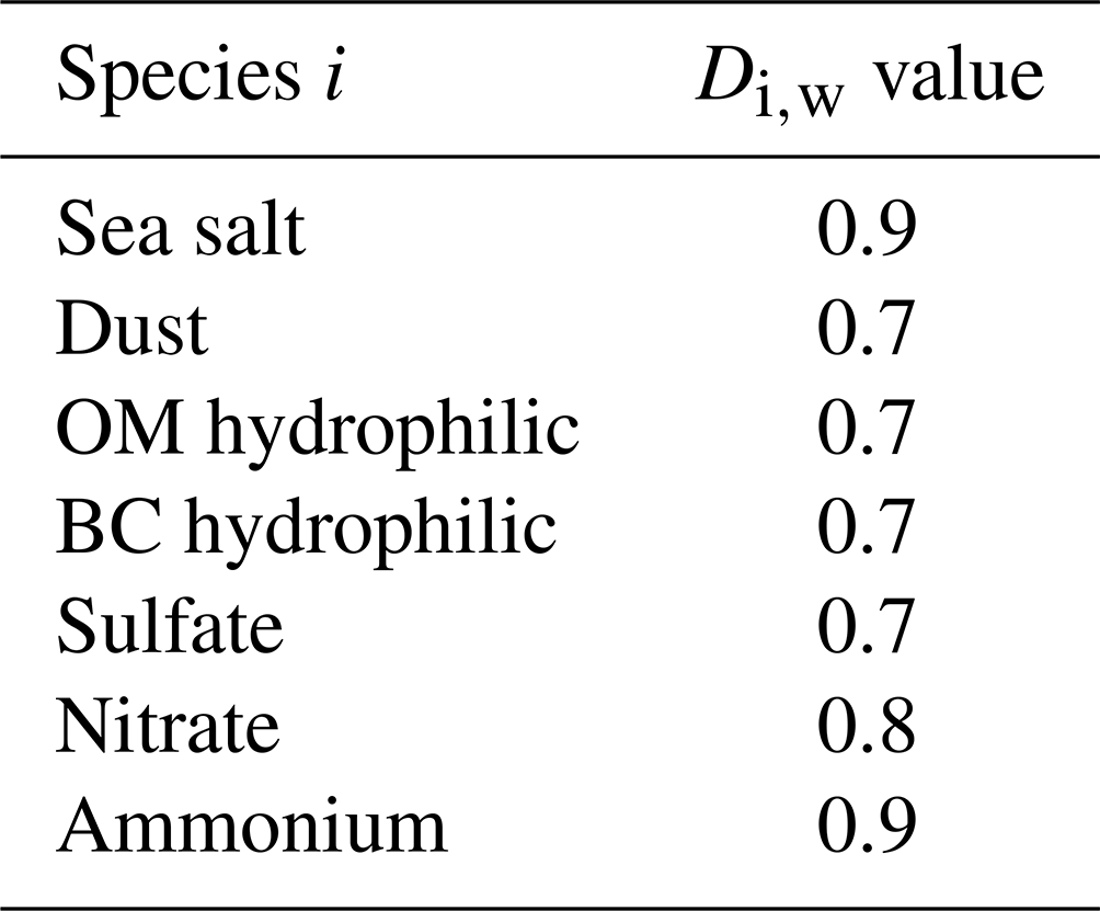
where Di is the in-cloud scavenging coefficient, defined as the fraction of the aerosol in the cloudy part of the grid box that is embedded in the cloud liquid and ice water. fk is the cloud fraction at level k. The value of the parameter Di is different for water and ice droplets: for water droplets, the values of Di,w from Table 7 are used, which have been derived from Reddy et al. (2005) and Stier et al. (2005). For ice droplets, Di,c is set to 0.06 for all aerosols following Bourgeois and Bey (2011). The final value of Di is computed from Di,w and Di,c by weighting them with the ice and water cloud droplet mass mixing ratio mc and mw, respectively:
Table 7Value of the parameter Dw, representing the fraction of the aerosol that is embedded in the cloud liquid water.
βk is the rate of conversion of cloud water to rain water. Before cycle 46R1, as described in Rémy et al. (2019), βk was computed following Giorgi and Chameides (1986), βk, by comparing the precipitation flux at levels k and k+1. In cycle 46R1, a new approach has been tested, using the cloud ice and water condensation fluxes instead:
where Cw,k and Cc,k are the cloud ice and water condensation fluxes at level k, qk is the sum of the liquid and ice mass mixing ratio, ρk is the air density at model level k, and Δzk is the layer thickness of the model level k
The representation of the re-evaporation process has also been made more complex. The release of aerosol particles contained in rain drops at level k occurs if evaporation of precipitation is diagnosed, i.e. if the precipitation flux at level k is higher than at level k+1, where level k+1 is below level k. If there is no precipitation at level k+1, then all aerosols that have been subjected to in-cloud scavenging at or above level k are released. If the precipitation flux at level k+1 is not null, the re-evaporation is partial. Before cycle 46R1, it was arbitrarily assumed that half of the scavenged aerosols at or above level k are then released. Since cycle 46R1, a more complex parameterisation has been implemented, following de Bruine et al. (2018). The mass of an aerosol species i that is re-evaporated at level k is computed as a function of the fraction of evaporated precipitation defined with the precipitation flux at level k Pk, :
where is the sum of the mass of aerosol that is subjected to in-cloud wet deposition from level k to the model top.
5.2.2 In-cloud scavenging in cycle 47R1
In cycle 47R1 a new optional formulation of the in-cloud scavenging rate has been implemented that is not yet used operationally for technical reasons but is used in operational cycle 47R3. This formulation is adapted from the approach of Luo et al. (2019). For liquid precipitation,
where k in s−1 is the first-order rainout loss rate Giorgi and Chameides (1986), which represents the conversion of cloud water to precipitation water. represents the condensed water content (liquid) within the grid cell. Pr is the rate of new precipitation formation (rain only) in the corresponding grid box. fk is the cloud fraction at level k. is derived from the liquid water mass mixing ratio qk by , where δt is the time step. βr,k is defined as in Giorgi and Chameides (1986) using the rain flux at level k Pr,k:
The rainout loss rate is computed as follows:
where Di,w is the fraction of aerosol that is embedded in the cloud liquid or solid water provided by Table 7 and Kmin is the minimum value of rainout loss rate, set to 0.0001 s−1 in Luo et al. (2019). Finally, the in-cloud scavenging rate in liquid cloud water is expressed as follows:
The formulation of Luo et al. (2019) applies only to liquid precipitation. It has been extended for solid precipitations but taking into account the smaller fraction of aerosols included in solid precipitations; the value of the Di parameter is divided by 2 for solid precipitation. The scavenging rates for both solid and liquid precipitation are then added.
5.2.3 Below-cloud scavenging in cycle 46R1 and 47R1
Since cycle 46R1, the below cloud scavenging rate is expressed by
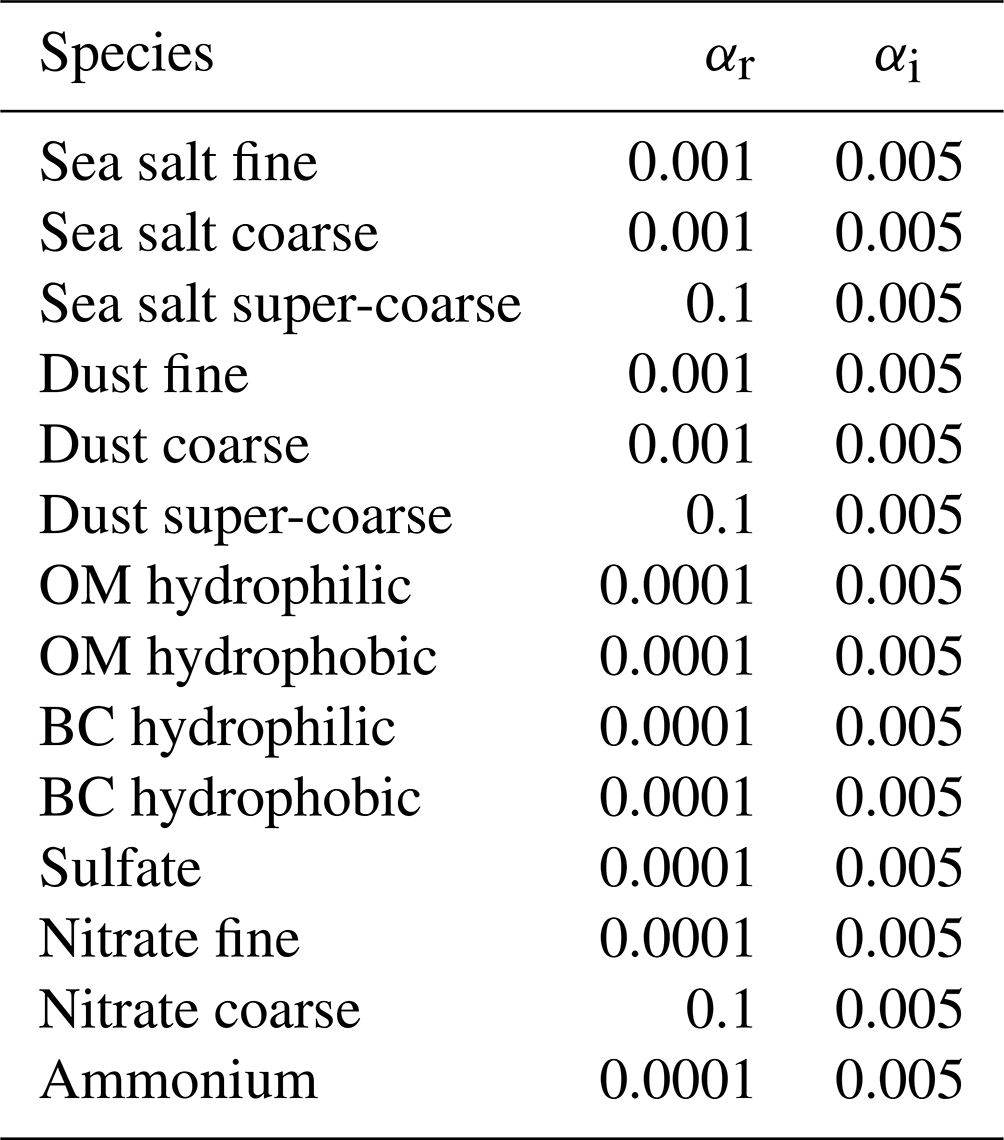
where Pr,k and Pi,k are the fluxes of liquid and solid precipitation, respectively, fpk is the fraction of grid cell at level k in which precipitation occurs, and αr and αi are the efficiency with which aerosol variables are washed out by rain and snow, respectively. The values used have been derived from Croft et al. (2009) and are summarised in Table 8.
5.3 Sedimentation
The computation of sedimentation fluxes is unchanged from Rémy et al. (2019) and Morcrette et al. (2009). However, since cycle 47R1 it has been applied to coarse sea salt aerosol in addition to the super-coarse sea salt and dust aerosols. Moreover, the sedimentation velocity is computed dynamically using Stokes's law as a function of particle size and density, which themselves vary as a function of relative humidity for sea salt aerosol:
where ρp,RH and rp,RH are the particle density and radius, respectively, that depends on relative humidity, g is the gravitational constant, μ is the air viscosity, and CF is the Cunningham correction factor.
6.1 Configuration of the IFS-AER simulations
IFS-AER was run in cycling forecast mode without data assimilation from January to December 2017 at a resolution of TL511L137, using emissions and model options similar to the operational CY47R1 run. Simulations have been carried out for cycle 45R1 without coupling to the chemistry and for cycle 47R1 with the operational set of deposition options (denoted “CY47R1”), the wet deposition adapted from Luo et al. (2019) and dry deposition adapted from Zhang and He (2014) (denoted as “CY47R1_NEWDEP”). The two CY47R1 and CY47R1_NEWDEP experiments use IFS-AER coupled to IFS-CB05. In order to assess the model skill independently of resolution and emission inputs, the three simulations, 45R1, 47R1 and 47R1_NEWDEP, used the same horizontal and vertical resolution and the same emission inputs.
6.2 Observations used
A broad range of observational datasets have been used to evaluate the IFS-AER simulations.
6.2.1 In situ
AOD data from the Aerosol Robotic Network (AERONET; Holben et al., 1998) are used to validate IFS-AER forecasts. AERONET level 2 data (cloud screened and quality assured with final calibrations) are used rather than level 1.5. We focus here on AOD at 500 nm. The Maritime Aerosol Network (MAN, Smirnov et al., 2009) component of AERONET provides ship-borne aerosol optical depth measurements from the Microtops II sun photometers. These data provide an alternative to observations from islands and establish validation points for satellite and aerosol transport models. Since 2004, these instruments have been deployed periodically on ships of opportunity and research vessels to monitor aerosol properties over the world's oceans.
PM2.5 and PM10 observations are provided by the AirNow database (https://www.airnow.gov/about-airnow/, last access: 4 February 2022) over North America, the European Environment Agency (EEA) over Europe and the China National Environmental Monitoring Center over China. For these three regions, special care was taken to use only rural background stations. Observations of speciated aerosol surface concentration from two datasets have been used: the Clean Air Status and Trends Network (CASTNET; https://www.epa.gov/castnet, last access: 20 June 2021) over the US and the European Monitoring and Evaluation Programme (EMEP, https://ebas.nilu.no/, last access: 16 June 2021) over Europe. The CASTNET network is operated by the U.S. Environmental Protection Agency (EPA). The ambient concentrations of gases and particles are collected with an open-face three-stage filter pack at CASTNET sites and a three-stage filter pack or bulk samplers at EMEP sites. The two networks also provide observations of wet deposition of sulfur and nitrogen constituents (both particulate and gaseous). Weekly ambient concentrations of gases and particulate species, including HNO3, SO4, NO3 and NH4, are available from 93 CASTNET sites in 2017. Daily observations of ambient concentration of selected trace gases and aerosol species, including SO4, NO3 and NH4, are available from 37 EMEP stations. In this work, only surface sulfate evaluation is presented.
The Interagency Monitoring of Protected Visual Environment (IMPROVE) programme was initially established in the US as a national visibility network in 1985 and consisted of 30 monitoring sites primarily located in national parks. The network expanded significantly in the late 1990s, and the measurements were diversified to also include some aerosol constituents such as surface concentrations of elemental carbon (or black carbon, BC) and organic carbon (OC) included in PM2.5. The use of identical samplers and analysis protocols by the same contractors ensures that data generated by IMPROVE and IMPROVE protocol sites can be treated as directly comparable. The 3-daily data are available from 150 sites in 2017. In this paper we did not use the sites located in mountains in order to avoid possible representativity issues as our model resolution is quite coarse. We used data only from sites that are below 500 m in altitude, which numbered 50 in 2017.
6.2.2 Remote sensing
As described in Sogacheva et al. (2020), a 1∘ × 1∘ gridded monthly AOD at 550 nm merged product for the period 1995–2017 was built from 12 individual satellite AOD products retrieved from AVHRR, SeaWiFS, (A)ATSR, MODIS Terra and Aqua, MISR, POLDER, and VIIRS. Different merging approaches were applied, and the resulting AOD was evaluated against AERONET. Optimal agreement of the AOD merged product with AERONET further demonstrates the advantage of merging multiple products. The quality of the merged product is as least as good as that of individual products. The temporal and spatial coverage of the merged product is better than one from the individual products, which makes it a very suitable remote sensing AOD product to compare against simulated AOD at 550 nm.
In order to evaluate the simulated dust AOD at 550 nm, the MODIS Dust AeroSol (MIDAS) dataset was used (Gkikas et al., 2020). MIDAS provides columnar daily dust optical depth (DOD) at 550 nm at a global scale and fine spatial resolution (0.1∘ × 0.1∘) over a 15-year period (2003–2017). This new dataset combines quality-filtered satellite aerosol optical depth (AOD) retrievals from MODIS-Aqua at swath level (collection 6.1, level 2) and DOD-to-AOD ratios provided by the Modern-Era Retrospective analysis for Research and Applications version 2 (MERRA-2, Gelaro et al., 2017) reanalysis to derive DOD on the MODIS native grid.
Observations of dust deposition are relatively sparse. Some are available from a few sites over the Western Mediterranean as described in Vincent et al. (2016) or those collected at the Izaña Global Atmospheric Watch Observatory in the Canary Islands by Waza et al. (2019). An estimate of African dust deposition flux and loss frequency (a ratio of deposition flux to mass loading) along the transatlantic transit is provided by Yu et al. (2019) using the three-dimensional distributions of aerosol retrieved by spaceborne lidar (Cloud–Aerosol Lidar with Orthogonal Polarization, CALIOP) and from AOD products from MODIS, MISR and IASI. Yu et al. (2019) convert the observed AOD into dust mass using assumed values of dust mass extinction efficiency (MEE). Because MEE is strongly dependent on the dust density and particle size distribution (Mahowald et al., 2014), Yu et al. (2019) assume that dust MEE increases linearly with dust transport distance, from 0.37 m2 g−1 near the African coast (east of 20∘ W) to 0.60 m2 g−1 at 100∘ W to account for possible preferential removal of larger dust particles during transport.The dust deposition fluxes are then derived from the difference of inbound and outbound dust mass fluxes for each grid cell over the North Atlantic using winds from MERRA-2 and assuming no leak at the top of the atmospheric column. This results in an estimate of seasonal total (dry+wet) dust deposition over 2∘ × 5∘ grid cells in the North Atlantic averaged over 2007–2016.
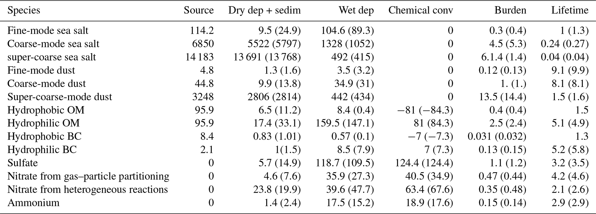
Table 9CY47R1 IFS-AER mean budgets of dry aerosols for 2017 (fluxes are expressed in Tg yr−1, burdens in Tg and lifetimes in d). Values from the CY47R1_NEWDEP experiments are shown in parentheses.
6.3 Budgets
Budgets are presented in Table 9 for the two cycle 47R1 experiments. For both sea salt and dust, the particle size has an important impact on lifetime: the larger particles have a much shorter lifetime because of more active dry deposition and sedimentation. Compared to results from cycle 45R1 presented in Rémy et al. (2019), the lifetime of fine and coarse dust aerosols are noticeably longer, probably because of changes in wet deposition, which is dominant for these two bins. Similarly, the lifetime of the other fine species, OM, BC and sulfate, are significantly longer than simulated with CY45R1; as wet deposition is the dominant sink for these species, these changes are mainly caused by the updates in wet deposition. For the biomass burning contribution of BC and OM, the use of injection heights for emissions could also contribute: when emitted at surface, biomass burning OM and BC is immediately subjected to dry deposition, which is not the case when it is emitted aloft.
The values indicated in Table 9 can be compared against the values from the AeroCom Phase III control experiment, as reported in Gliß et al. (2021), which also includes data from IFS-AER cycle 46R1. The objective of the AeroCom initiative is to document differences in aerosol component modules of global models and to assemble datasets for model evaluations. A total of 14 global models participated to the Phase III control experiment, which consisted of simulating aerosols for the years 1850 and 2010. All models used the same CMIP6 emissions. The AeroCom median refers to the 2010 experiment. Because the AeroCom experiments are for 2010 and used a different set of emission inputs, the median is not fully comparable to values provided by IFS-AER simulations of the year 2017. However, they give an indication of how IFS-AER broadly compared to other global aerosol models.
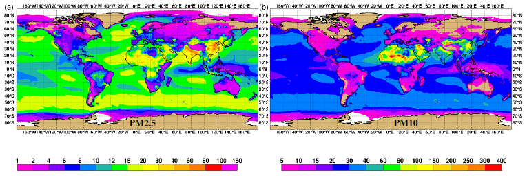
Figure 3Global mean 2017 PM2.5 (a) and PM10 (b) (in µg m−3) simulated by the CY47R1_NEWDEP experiment in cycling forecast mode. Please note the different scales for PM2.5 and PM10.
For the sum of the emissions of dry sea salt aerosol (i.e. divided by the factor 4.3) for the three bins stands at 21 147 Tg yr−1, which is much higher than the AeroCom median (4980 Tg yr−1) and is the highest of all models reported in Gliß et al. (2021), except for IFS-AER cycle 46R1 at more than 50 000 Tg yr−1, which used the Grythe et al. (2014) sea salt aerosol emission scheme. This value is heavily influenced by the cutoff radius for sea salt aerosol, which at 20 µm at 80 % RH is probably one of the highest. The lifetime of sea salt aerosol is also the lowest of all models for similar reasons: super-coarse sea salt with a very short lifetime is much more abundant than the other sea salt aerosol bins, which show a relatively longer lifetime. Nevertheless, the fact that the lifetime of simulated sea salt aerosol is significantly lower than all other models may be a sign that sinks are too active in IFS. The fact that sea salt aerosol lifetime is increased with the new deposition options also agrees with this conclusion.
For dust, the total emissions are simulated to reach 3297.6 Tg yr−1 with IFS-CY47R1, lower than the 5650 Tg yr−1 reported in Gliß et al. (2021) with IFS-AER cycle 46R1. This lower value is caused by the update of the dust source function that occurred in cycle 47R1, as mentioned above. The cycle 47R1 emissions are significantly higher than the AeroCom phase III median (1440 Tg yr−1) and are above all other models, as was the case for sea salt aerosols. Similar to the results for sea salt aerosol, this could be because the cutoff radius (20 µm dry radius) is higher than most models. The lifetime of simulated dust stands at 1.5 d with cycle 47R1, which is much lower than the AeroCom phase III median. The most likely explanation is that the bulk of simulated dust with IFS-AER is super-coarse dust, both because of the high cutoff diameter and because the size distribution of emitted dust follows Kok (2011), with more emissions of super-coarse dust relative to other size distributions of dust.
Organic matter emissions are also among the highest reported in Gliß et al. (2021) at 192 Tg yr−1. This probably comes from the SOA components, as relatively few models directly emit SOA as a fraction of organic matter. The lifetime is simulated to be 4.6 d, shorter than the AeroCom phase III median (6 d) but within its bounds, as 4 models out of 13 (excluding IFS-AER cycle 46R1) simulate shorter lifetimes for organic matter. For black carbon, there is a higher level of consensus for the emissions, which are very close between all models. The simulated lifetime, 4.4 d, is slightly lower than the AeroCom median (5.5 d). For both organic matter and black carbon, the new deposition options bring an increase in simulated lifetime, which reduce the difference with the AeroCom median.
Chemical production of sulfate (124 Tg yr−1) is quite close to the AeroCom median (143 Tg). The simulated lifetime (3.2 d) is shorter than the AeroCom median (4.9 d). For nitrate production (103.9 Tg yr−1), the IFS-AER cycle 47R1 value is among the highest and is much higher than the AeroCom median value of 32.5 Tg yr−1. However, the variability between AeroCom models is very high, which is partly explained by the fact that some include nitrate production from heterogeneous reactions of dust and/or sea salt aerosol particles (IFS-AER represents both sources). As for most species, the simulated lifetime of nitrate (3 d) is shorter than the AeroCom median (3.9 d), but the variability is also high for this parameter.
6.4 Simulated AOD at 550 nm and particulate matter (PM)
6.4.1 PM2.5 and PM10
Figure 3 shows the global PM2.5 and PM10 simulated by the CY47R1_NEWDEP experiment for 2017. It can be compared to Fig. 11 of Rémy et al. (2019). For PM2.5, maximum values of up to 60–70 µg m−3 are simulated over parts of China and India, mostly from anthropogenic aerosols, and over parts of the Sahara, mostly from desert dust. Over oceans, the mean values vary between 8 and 20 µg m−3. Over Europe and the eastern US, the simulated values vary between 6 and 12 µg m−3. Areas of seasonal biomass burning such as equatorial Africa, parts of Brazil and Indonesia show simulated PM2.5 between 10 and 20 µg m−3 on a yearly average. Individual large fire events, such as the “British Columbia” fire of August 2017 also appear over western Canada, lifting the yearly average there to 10–15 µg m−3.
Dust and sea salt aerosols are much more prominent in Fig. 3b. Over oceans, the simulated PM10 varies between 20 and 35 µg m−3, while yearly values can reach up to 200–300 µg m−3 over the dust-producing regions of the Sahara, Arabian Peninsula and the Taklamakan desert. PM10 over the heavily polluted areas of India and China reaches 80–100 µg m−3, which is only 20–30 µg m−3 more than PM2.5 over these regions, which are impacted mainly by fine particles. Similarly, the simulated PM10 values over Europe, US and the seasonal biomass burning regions are 20 %–30 % higher than the PM2.5 values.

Figure 4Mean 2017 total (a), dust (b), sea salt (c), OM (d), BC (e), sulfate (f), nitrate (g) and ammonium (h) AOD at 550 nm simulated by the CY471_NEWDEP experiment.
Table 10Average over 2017 of the modified normalised mean bias (MNMB)/fractional gross error (FGE) of simulated daily AOD at 500 nm. PM2.5 and PM10. AOD observations are from AERONET level 2. European PM observations are from 65 PM2.5 and 138 PM10 background rural airbase stations. North American PM observations are from 125 PM2.5 stations and 25 PM10 background rural stations. Chinese PM observations are from 152 PM2.5 background rural stations.
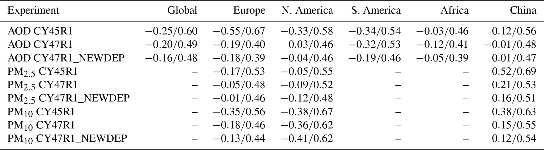
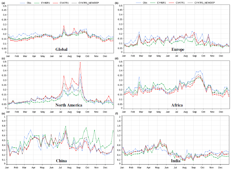
Figure 5Global (a) and regional (b)–(f) simulated vs. observed level 2 weekly AOD at 500 nm from AERONET averaged over 7 d.
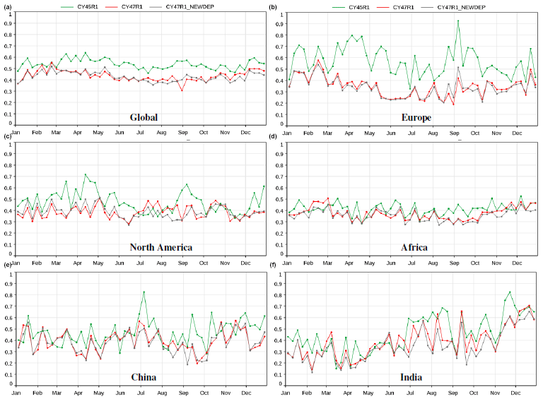
Figure 6Fractional gross error (FGE) of simulated weekly AOD at 500 nm against global (a) and regional (b)–(f) level 2 AOD from AERONET.
6.4.2 AOD at 550 nm
Figure 4 shows total and speciated AOD at 550 nm simulated by the CY47R1_NEWDEP experiment for 2017. The highest values can be found in the heavily populated regions of the Indian subcontinent and eastern China; the dust-producing regions of the Sahara, the Arabian Peninsula, and the Taklamakan desert; and in the seasonal biomass burning region of equatorial Africa. The transport of dust produced in the western Sahara and over the Taklamakan and Gobi deserts over the Atlantic and Pacific, respectively, are prominent features that can be used to assess the deposition processes. Sea salt AOD is quite evenly spread between the mid-latitude regions, where mean winds are high, and the tropics, where trade winds are on average less intense but have a relatively more active sea salt production thanks to the dependency of sea salt production on SST. OM is a species that combines anthropogenic and biomass burning sources: AOD is highest over parts of China and India, mostly from secondary organics scaled on anthropogenic CO emissions, and over equatorial Africa, from biomass burning. BC sources are also a combination of anthropogenic and biomass burning origin, the patterns are close to what is simulated for OM. Sulfate AOD is concentrated over heavily populated areas, and a few outgassing volcanoes such as Popocatépetl in Mexico and Kīlauea in Hawaii. Oceanic DMS sources bring a “background” of sulfate AOD over most oceans. Nitrate AOD is highest over the regions where anthropogenic emissions of nitrogen oxides are highest, i.e. over India and China. Some secondary maxima also appear over seasonal biomass burning regions from biomass burning emissions of nitrogen oxides. Finally, the features of ammonium AOD are close to those of nitrate AOD but with lower values.
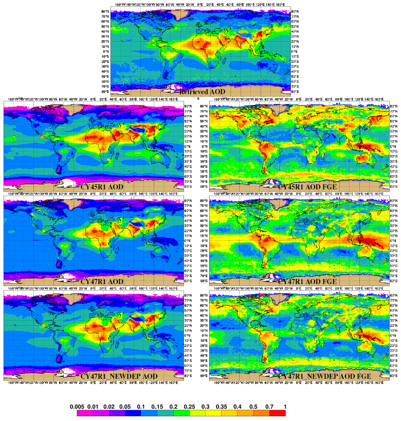
Figure 7The top panel shows the 2017 average of merged AOD at 550 nm from Sogacheva et al. (2020). The left column shows the co-located simulated yearly AOD for CY45R1, CY47R1 and CY47R1_NEWDEP from top to bottom. The right column shows the fractional gross error of simulated AOD against the merged AOD product for CY45R1, CY47R1 and CY47R1_NEWDEP from top to bottom.
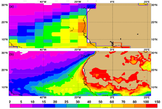
Figure 8(a) The 2007–2016 mean dust total deposition (in ) as estimated by MODIS. (b) The mean 2017–2019 dust total deposition as simulated by IFS-AER cycle 47R1 without data assimilation (in ).
6.5 Evaluation summary
Table 10 shows a summary of global and regional skill scores for AOD at 500 nm and PM for a year of simulation of the CY45R1, CY47R1 and CY47R1_NEWDEP experiments. The modified normalised mean bias (MNMB) and fractional gross error (FGE) are shown so that the metrics are not too impacted by a few local extreme events, as can be the case with bias and root-mean-square error (RMSE). MNMB varies between −2 and 2; it is defined for a population of N forecasts fi and observations oi by the following equation:
FGE varies between 0 (best) and 2 (worst) and is defined as follows:
The AOD at 500 nm as simulated by CY45R1 shows a negative MNMB globally and over all regions except China, ranging from −0.03 over Africa to −0.55 over Europe. The FGE is above 0.5 for all regions except Africa. CY47R1 clearly improves the MNMB: the negative values are reduced everywhere except Africa and range from −0.12 over Africa to −0.32 over South America. FGE is below 0.5 for all regions except South America. The new deposition options of CY47R1_NEWDEP bring a further improvement to the MNMB, which measured between 0.01 over China and −0.19 over South America. FGE is also improved marginally by NCY47R1_NEWDEP compared to CY47R1: it is reduced by 0.01–0.02 over all regions except South America where the improvement is more noticeable (0.07).
The PM2.5 evaluation has only been carried out over Europe, North America and China using only background rural stations.
PM10, similar to PM2.5, shows a significant improvement in MNMB and FGE over Europe and China and a lower improvement over the US.
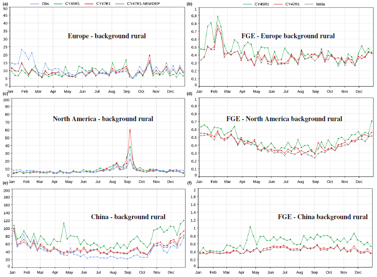
Figure 9The left column shows observed and simulated weekly PM2.5 over Europe (background rural, a), North America (background urban, c) and China (all sites, e). The right column shows the fractional gross error (FGE) of simulated PM2.5 against observations.
6.6 Evaluation against AERONET
Figures 5 and 6 show two measures of skill of the simulated weekly AOD at 500 nm against global and regional AERONET observations: bias and fractional gross error (FGE). There is generally a global negative bias of simulated AOD against AERONET values on the order of 0.02–0.03 with CY45R1. This negative bias is slightly worsened by CY47R1 and slightly improved by CY47R1_NEWDEP. The FGE is generally improved by the two CY47R1 experiments. In July and August 2017, large fires in the US and Canada provoked spikes in simulated and observed AOD (consisting mainly of organic matter AOD). The FGE is not impacted, but the RMSE (not shown) is very high during these 2 months over North America. The regional skill scores against AERONET are more varied. Over Europe, a 0.05 negative bias with CY45R1 is significantly improved with the two CY47R1 experiments (0.02 negative bias) and associated with a reduced FGE, which is generally between 0.5–0.7 with CY45R1 and below 0.5 with the two CY47R1 experiments. Several factors can explain this improvement; the dominant cause is probably the presence of nitrate/ammonium aerosols in the CY47R1 experiments. Over North America, the simulated negative bias with CY45R1 turns to a small positive bias with 47R1 and is at times very large during fire events in July–August and December. The positive bias of CY47R1 over North America is much improved with CY47R1_NEWDEP, which shows a nearly null mean bias. The FGE is often improved with CY47R1_NEWDEP compared to CY45R1. This increase in simulated biomass burning aerosols could be caused by changes in deposition, as there are no changes in the GFAS emissions used between the three experiments. It is very likely that the use of injection heights for biomass burning emissions in the two CY47R1 experiments also plays a role. Over Africa, the bias of CY45R1 against AERONET is smaller than over other regions. CY47R1 shows a larger negative bias of 0.05, which is in turn reduced by CY47R1_NEWDEP. Besides other changes, the implementation of the new dust emission scheme probably plays a significant role regarding the changes in the skill scores over Africa. The FGE of simulated AOD at 500 nm is generally improved compared to CY45R1 (more so with CY47R1_NEWDEP) with values generally between 0.4 and 0.5. There is little difference between the two CY47R1 experiments over China; the CY45R1 experiment shows a significant positive bias after August 2017. The bias is generally quite small with the two CY47R1 experiments, and FGE is generally improved (sometimes significantly, such as in summer). For the September–December 2017 period, RMSE (not shown) is nearly halved. Finally, CY45R1 displays a significant negative bias of 0.2 on average over India. This bias is more than halved with the two CY47R1 experiments. The impact on FGE is generally positive.
6.7 Evaluation against remote sensing products
6.7.1 AOD
In order to assess the relative error of the simulated AOD at 550 nm compared to the merged AOD at 550 nm product from Sogacheva et al. (2020), the fractional gross error (FGE) is used, and thus the errors of the model in simulating relatively low values are not overlooked compared to the larger errors that occur in regions where AOD is usually higher, such as over deserts and biomass burning regions.
Figure 7 shows co-located retrieved and simulated AOD at 550 nm together with the fractional gross error of the simulated AOD. Over most oceans, CY45R1 is generally the closest to the merged AOD product, but the changes in wet and dry deposition of CY47R1_NEWDEP bring a significant increase in simulated AOD compared to CY47R1. The improved skill of the new sea salt aerosol emission schemes shows in the FGE plots, which are significantly improved compared to CY45R1 over most of oceans with CY47R1 (and even more so with CY47R1_NEWDEP). Over most regions, the FGE of CY47R1_NEWDEP is lower than CY47R1. The decrease in FGE between CY45R1 and CY47R1 is not general: it concerns most of Europe, China, Canada, and Russia; a majority of oceans; and the western Sahara. A few areas show a degradation in FGE, i.e. parts of the eastern Sahara, Indonesia and the central Pacific.
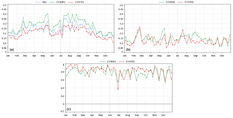
Figure 10(a) Observed and simulated weekly averaged AOD in 2017 over a selection of 24 AERONET stations more representative of desert conditions. (b) RMSE of simulated AOD against AERONET AOD at these 24 stations. (c) Spatial correlation between simulated and observed AOD at 500 nm. The AERONET stations used in this plot are: Tizi Ouzou, Tamanrasset INM, Sede Boker, Mezaira, Masdar Institute, Lampedusa, KAUST Campus, Izana, Tunis Carthage, Ilorin, Santa Cruz de Tenerife, La Laguna, Dakar, Dalanzadgad, Cairo EMA, Dushanbe, Arica, Gobabeb, Windpoort, Ben Salem, Cabo Verde, La Parguera, Teide, El Farafra.
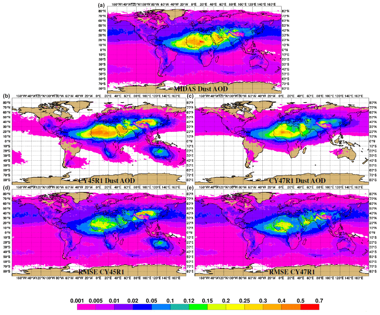
Figure 11(a) The 2017 average MIDAS dust AOD at 550 nm. Co-located 2017 average of dust AOD at 550 nm simulated by IFS-AER CY45R1 (b) and CY47R1 (c). The 2017 average daily RMSE of simulated dust AOD at 550 nm for CY45R1 (d) and CY47R1 (e).
6.7.2 Dust deposition
Figure 8 shows a comparison of this climatological dust deposition against values simulated by a long-cycle 47R1 cycling forecast (i.e. without data assimilation) experiment, which uses a configuration similar to CY47R1_NEWDUST. Overall, despite a local underestimation of the simulated dust deposition, the retrieved and simulated values match very well, which is a good indicator that IFS-AER manages to capture the climatological deposition of dust relatively well. However, it seems that deposition is overestimated close to the African coastline and underestimated in the western Atlantic, a sign that transatlantic transport of dust is possibly underestimated by IFS-AER.
6.8 Evaluation against PM2.5 observations
PM2.5 is a key product provided by the global CAMS service. As such, its evaluation is of special importance. Observed PM2.5 has been gathered from three geographical areas: Europe, North America and China. Over China, the site classification (rural or urban and background or traffic) is not known, and thus the statistics probably include many sites that are not really suitable for comparison against simulations by a global model with a relatively coarse horizontal resolution.
Over the background rural stations of Europe, PM2.5 simulated by CY45R1 displayed a significant negative bias of 2–5 µg m−3 in general, reaching more than 10 µg m−3 in January–February 2017. This period of the year 2017 witnessed a severe cold wave across much of Europe, which was probably associated with higher levels of residential wood burning and thus anthropogenic aerosol emissions. This kind of impact of meteorological parameters on emissions is currently not taken into account. The negative bias over Europe by CY45R1 is significantly improved by the two CY47R1 experiments, which simulated PM2.5 2–3 µg m−3 higher than CY45R1 in winter months. The negative bias in January and February 2017 is decreased by CY47R1 but far from eliminated. CY47R1_NEWDEP is generally close to CY47R1, except in August and mid-October 2017. The mid-October 2017 spike in PM2.5 is associated with the large fires that struck Portugal. The RMSE of CY47R1_NEWDEP (not shown) is much lower than CY47R1, which shows that the new deposition options have a beneficial impact on the skill of simulated biomass burning plumes. Generally speaking, the FGE of CY47R1 is significantly better than that of CY45R1, with a decrease of 0.1–0.2 in general. RMSE (not shown) shows a larger relative improvement in summer, when the error is at times more than halved.
The overall picture is slightly different over the background rural stations of North America, where the simulated PM2.5 by CY45R1 shows little bias in winter months but a significant positive bias of 2–3 µg m−3 on average during summer months. As in Europe, the simulated PM2.5 is generally lowered by 1–2 µg m−3 in general when using the CY47R1 experiments, with even lower values during summer. This results in a small negative bias of 1–2 µg m−3 with CY47R1 from January to April 2017 and a generally small bias in the remaining months. The difference between CY47R1 and CY47R1_NEWDEP is mainly significant during summer, when CY47R1_NEWDEP is generally lower than CY47R1, and this is probably associated with biomass burning aerosols. A spike in simulated PM2.5 in early September 2017 with CY47R1 is associated with fire events. The significant positive bias of simulated PM2.5 by CY47R1 during this event is much improved by CY47R1_NEWDEP. As already noted over Europe, it seems that CY47R1_NEWDEP generally improves the skill of the model in simulating PM from fire events. The FGE of simulated PM2.5 is, as over Europe, significantly improved by the two CY47R1 experiments for all months.
Over China, CY45R1 overestimates simulated PM2.5 constantly and by a large margin from 20 µg m−3 to 40–60 µg m−3 from September to December 2017. On average, the simulated PM2.5 is twice as high as the averaged observations. The very high positive bias is significantly reduced by CY47R1, for which the positive bias does not exceed 20 µg m−3, and it is further reduced by 5–10 µg m−3 in the winter months by CY47R1_NEWDEP. The improvement with CY47R1 is largely explained by the improved representation of the sulfur cycle in CY47R1 associated with the coupling to IFS-CB05. In the end, CY47R1_NEWDEP shows little bias from January to April 2017, a significant positive bias of 10–20 µg m−3 from May to October, and a smaller bias for the rest of 2017. Associated with this large improvement in bias is a decrease of FGE with CY47R1 by 0.2–0.4 in CY47R1_NEWDEP. For the whole of 2017, the FGE of CY47R1_NEWDEP is decreased by up to 50 %, and the RMSE (not shown) is around 3 times lower than that over CY45R1. The absolute value is still high, at 30 µg m−3 on average, but this could also reflect the fact that many traffic stations are included in this dataset, for which there is a high representativity error when comparing against global forecasts at a 50 km horizontal resolution.
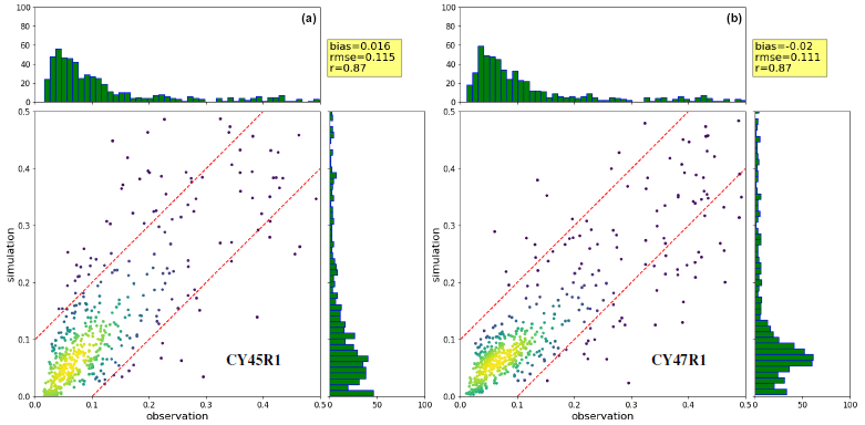
Figure 12Density scatterplot (for 2017) of AOD at 550 nm simulated by IFS-AER (a cycle 45R1, b cycle 47R1) and observed by the MAN network.
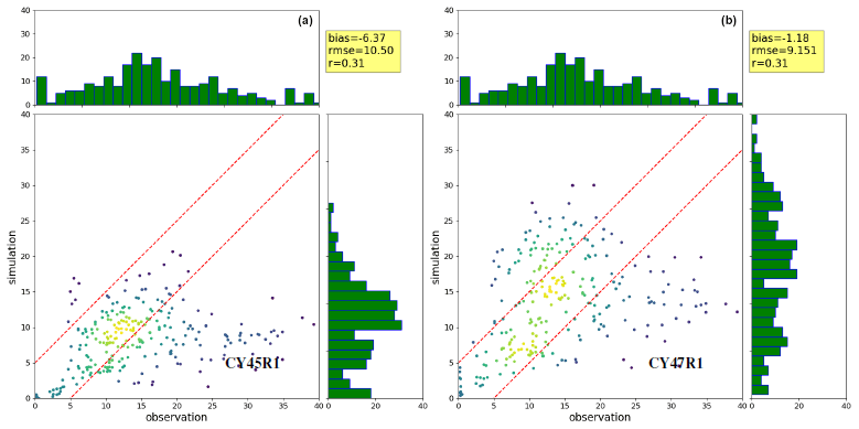
Figure 13Density plot (for 2017) of monthly simulated (a CY45R1, b CY47R1) sea salt surface concentration (in µg m−3; sum of bin1 and bin2) vs. climatological values from 21 AEROCE/SEAREX stations.
6.9 Evaluation of desert dust aspects
In order to evaluate and compare the skills of the two dust emission schemes, the simulated AODs at 500 nm as simulated by 45R1 (which uses the G01 scheme) and 47R1 (which uses the N12 scheme) have been compared against values observed at a selection of AERONET stations that are dominated by dust. Figure 10 shows such a comparison using RMSE instead of fractional gross error (FGE) as a metric of the forecast error because for an evaluation focusing on desert dust, focusing on large simulated values that correspond to extreme events is welcome. Despite higher emissions, the simulated dust AOD is significantly lower on average for the selected stations. A positive bias with the older scheme turns into a small negative bias. The skill of the simulated dust seems to improve with the new scheme, as RMSE is generally decreased and sometimes nearly halved, such as in August–September 2017 with a value of 0.1 instead of 0.2. The spatial correlation is also generally improved and stands above 0.9 most of the time with CY47R1, whereas it is frequently below this value with CY45R1.
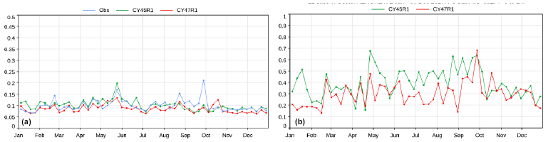
Figure 14(a) Observed and simulated AOD (averaged weekly) in 2017 over a selection of 14 AERONET stations more representative of sea salt aerosol. (b) Fractional gross error (FGE) of simulated AOD against AERONET AOD at these 14 stations.
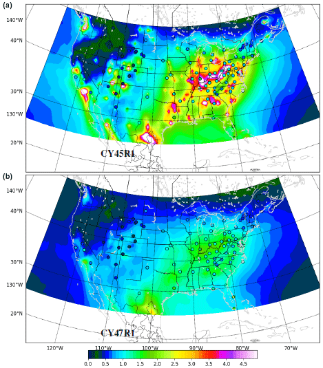
Figure 15Mean 2017 surface sulfate concentration (in µg m−3) simulated by CY45R1 (a) and CY47R1 (b) against the yearly average of the CASTNET network (shown as black circles).
The dust AOD simulated by IFS-AER CY45R1 and CY47R1 has been compared against daily dust AOD at 550 nm provided by the ModIs Dust AeroSol (MIDAS, Gkikas et al., 2020) dataset. Figure 11 shows the retrieved dust AOD at 550 nm averaged over 2017, as well as the co-located average as simulated by IFS-AER CY45R1 and CY47R1. The simulated dust AOD exhibits strong overestimation over the Taklamakan and Gobi region with CY45R1, as well as a less pronounced overestimation over most of the other dust-producing regions. With CY47R1, the simulated values are generally closer, as shown by the reduced averaged RMSE. Over a few areas, such as over the southern part of the Arabian Peninsula and the Atlantic Ocean, the RMSE is larger with CY47R1.
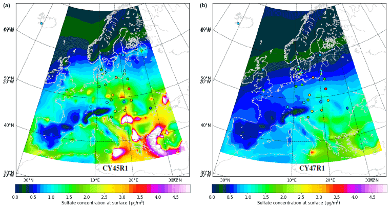
Figure 16Mean 2017 surface sulfate concentration (in µg m−3) simulated by CY45R1 (a) and CY47R1 (b) against yearly average from the EMEP network (shown as black circles).
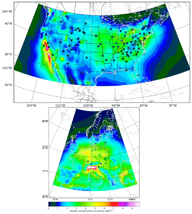
Figure 17Mean 2017 surface nitrate concentration (in µg m−3) simulated by IFS-AER CY47R1 against yearly average from the CASTNET and the EMEP networks (shown as black circles).
6.10 Evaluation of sea salt aerosol aspects
An evaluation of the new A16 scheme has been carried out against co-located AOD at 550 nm observations from the Maritime Aerosol Network (MAN, Smirnov et al. (2009)) against AOD at 550 nm from a selection of 14 AERONET (Holben et al., 1998) stations that are more representative of sea salt aerosols and against climatological monthly sea salt aerosol surface concentration observations from the AEROCE/SEAREX programme. The AERONET stations used are Ragged Point, Reunion St Denis, Noumea, Midway Island, Key Biscayne, Key Biscayne2, Cape San Juan, Edinburgh, Cabo da Roca, ARM Graciosa, American Samoa, Amsterdam Island, Andenes and Birkenes. Figure 12 shows the evaluation against total AOD at 550 nm from the MAN network. Total AOD provided by MAN cruises generally (but not always) consists mostly of sea salt aerosol optical depth. Occasionally, dust or biomass burning plumes can also have an impact, but this impacts a minority of the measurements. Figure 12 shows that a small positive bias of 0.016 of simulated AOD at 550 nm against MAN data turns into a small negative bias of −0.02, with little changes in correlation. The RMSE is slightly improved with CY47R1, decreasing from 0.115 to 0.111.
In order to assess the skill of simulated surface concentration of sea salt aerosol, observations of sea salt aerosol surface concentration carried out in the AEROCE and SEAREX programmes (Savoie et al., 2002) of the 1980s and 1990s are used as monthly climatologies. These observations were carried out by the University of Miami. As detailed in Jaeglé et al. (2011), these observations were carried out in ambient conditions with PM10 inlets, which is nearly consistent with the sum of bin1 and bin2 surface concentration (i.e. sea salt aerosols with a radius at 80 % relative humidity of up to 5 µm). Figure 13 shows that a small negative bias of 6.4 µg m−3 with CY45R1 is significantly reduced with CY47R1 and that RMSE is also lowered. The negative bias of CY45R1 may seem inconsistent with the positive bias in simulated AOD against MAN observations, but this apparent inconsistency can be explained by the fact that only the sum of bin1 and bin2 is used in the comparison against AEROCE/SEAREX data, whereas most of the sea salt aerosol emissions and burden in cycle 45R1 concern bin3, as shown in Table 5.
Finally, Fig. 14 compares simulated and observed AOD at 550 nm over a selection of 14 AERONET sites that are more representative of sea salt aerosol. The same remark can be made as for the MAN observations, i.e. that non-sea-salt aerosol probably contributes to some of the observed and simulated values and thus reduces the significance of this evaluation. However, with a careful selection of AERONET sites, it is likely that the contribution of non-sea-salt aerosols is much lower than that of sea salt aerosol. The improvement with CY47R1 is very clear, with a significantly reduced bias and a much improved FGE compared to CY45R1 (0.38 against 0.50), although correlation is low in both cases.
6.11 Evaluation against surface concentration observations
6.11.1 Sulfate
The impact of the coupling of IFS-CB05 and IFS-AER on simulated sulfate surface concentration is significant, as shown by Figs. 15 and 16. CY45R1 is standalone, while CY47R1 runs coupled with IFS-CB05. Over the US, sulfate is much overestimated by standalone IFS-AER at the surface against observations; this positive bias is largely eliminated with coupled IFS-AER. Over Europe, the improvement is less clear, but the trend towards lower simulated sulfate aerosol with CY47R1 at surface is the same.
6.11.2 Nitrate
The sum of the simulated nitrate surface concentration from gas–particle partitioning and from heterogeneous reactions is compared against observations from the CASTNET and EMEP networks in Fig. 17. In general, nitrate from gas–particle partitioning is simulated over the considered regions to be much more abundant at the surface than nitrate from heterogeneous reactions. The experiment CY47R1_NEWDEP is not shown because the simulated values differ relatively little from those simulated by CY47R1. Over the US, the simulated surface concentration of nitrate is significantly higher than observations. Over much of the eastern US, the simulated values vary between 2 and 4 µg m−3 on average, while the observed values are generally in the range of 1–2 µg m−3. The simulated values are also significantly overestimated over large parts of Europe, with averages reaching 3–6 µg m−3 against observed values of 3–4 µg m−3 in general. This significant overestimation is a quite frequent feature of global models: it has been noted in GEOS-CHEM (Luo et al., 2019), GFDL (Paulot et al., 2016) and in the Met Office Unified Model (Jones et al., 2021), which has implemented an adapted version of the IFS-AER nitrate scheme. A number of factors can participate to this overestimation: too high particle production compared to the gas phase, which is likely over Europe where the simulated nitric acid surface concentration is much lower than observed; overestimation in the emissions or burden of gaseous precursors of nitric acid; or underestimation of the sinks. Following Paulot et al. (2016), simulations that apply the dry deposition velocity of nitric acid to nitrate have been carried out and were shown to significantly reduce the positive bias of simulated nitrate at surface. However these developments are recent and have not yet been included in operational IFS-AER.
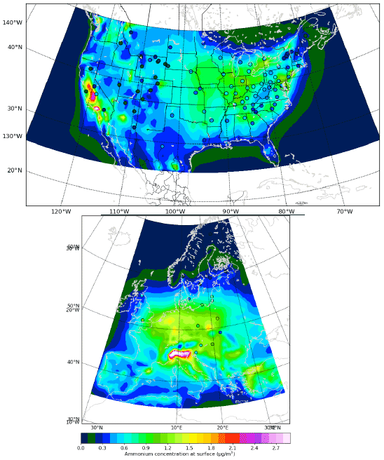
Figure 18Mean 2017 surface ammonium concentration (in µg m−3) simulated by IFS-AER CY47R1 against yearly average from the CASTNET and the EMEP networks (shown as black circles).
6.11.3 Ammonium
As for nitrate, the simulated surface concentration of ammonium is generally significantly overestimated over the US and Europe, as shown by Fig. 18. This comparison is not exactly representative, as ammonium from ammonium sulfate is part of the reported observations, while the ammonium species include only ammonium from ammonium nitrate. Over Europe, ammonia is also very much overestimated, which is not the case of the US. It is possible, at least over Europe, that the overestimation of ammonium can be partly explained by an ammonia burden that is too high, either from emissions that are too high or there being too little deposition.
6.11.4 Organic carbon
The IMPROVE network disseminates observations of the surface concentration of organic carbon included in PM2.5 over the US. Organic carbon has been derived from the hydrophilic and hydrophobic components of simulated organic matter by applying a 2.3 OM:OC ratio for the hydrophilic fraction and a 1.4 ratio for the hydrophobic one. These values are used by the EPA to convert organic matter from CAMS products into organic carbon (Christian Hogrefe, personal communication, 2019). This is a strong assumption, as these ratios are known to vary a lot depending on the aerosol source, transport, ageing, etc. El-Zanan et al. (2005) found a mean value of 2.07 for the OM:OC ratio over all IMPROVE sites using data from 1988 to 2003, which is consistent with our values. The fraction of organic carbon in PM2.5 is derived from the surface concentration of organic carbon by applying a 0.7 factor, consistent with the PM2.5 formula used in IFS-AER, which relates to the assumed size distribution of the organic matter species.
Figure 19 shows simulated and observed organic carbon in PM2.5 for the three CY45R1, CY47R1 and CY47R1_NEWDEP experiments. The simulated values are very much overestimated with CY45R1, reaching 4–6 µg m−3 on average in the south-east, while observations are in the range of 2 µg m−3. In the west, spikes of simulated very high values, above 10 µg m−3 correspond to fire events. There are no such spikes in the observed values. The simulated surface concentration of OC in PM2.5 is significantly reduced with CY47R1. As the emissions are the same, this can be explained by the use of injection heights for biomass burning emissions and is possibly an impact of the new scavenging scheme. Despite this decrease, the simulated values are still generally higher than the observations, e.g. 3–5 µg m−3 in the south-east. The spikes associated with fires are smaller in extent but are still present. These spikes are largely reduced with CY47R1_NEWDEP, which is consistent with the conclusions from the evaluation against PM2.5 observations, where a strong impact of the new deposition options on simulated PM2.5 from biomass burning origin was noted. CY47R1_NEWDEP bring a further significant decrease in simulated surface organic carbon in PM2.5 over the whole of the US. Despite this, the simulated values are still generally higher than the observations. This could be explained by the fact that secondary organic aerosols, which represent a large fraction of the emissions of organic matter, are released at the surface, while in reality they are produced by reactions aloft.
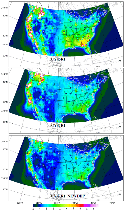
Figure 19Mean 2017 surface concentration of organic carbon in PM2.5 (in µg m−3) simulated by IFS-AER CY47R1 against the yearly average from the IMPROVE network (shown as black circles).
Figure 20Simulated vs. retrieved wet deposition flux of sulfur over the United States for 2017.
6.12 Evaluation of wet deposition fluxes against CASTNET data
Evaluating and constraining the deposition processes is an indispensable step in the development of IFS-AER and any global aerosol model. There is also a wide interest in the evaluation of sulfur and nitrogen (S and N) deposition fluxes, which are generally dominated by wet deposition. Sulfur dioxide and sulfate aerosols impact the acidity of precipitation (Myhre et al., 2017), while oxidised nitrogen aerosols and gases (NO3, HNO3 and reduced nitrogen aerosols and gases (NH4 and NH3) act as powerful plant and microorganisms nutrients when deposited to terrestrial and aquatic ecosystems. On the other hand, excessive input of nitrogen can lead to eutrophication and loss of ecosystem biodiversity and productivity (Fowler et al., 2015)
Because of this high impact, S and N deposition fluxes are the subject of numerous studies, particularly within the framework of the Task Force on Hemispheric Transport of Air Pollution (HTAP) of the World Meteorological Organization (Tan et al., 2018; Vet et al., 2014). Regionally over Europe, the Eurodelta Trends model intercomparison exercise also focused on S and N deposition fluxes (Theobald et al., 2019). IFS-AER coupled with IFS-CB05 is well placed to simulate the gaseous and aerosol components of the S and N deposition fluxes. An exhaustive evaluation of simulated S and N deposition fluxes against the global dataset provided by Vet et al. (2014) has been carried out but is out of scope for this paper. Here, we present an evaluation of the simulated S wet deposition flux.
The simulated sulfur wet deposition fluxes for 2017 are shown in Fig. 20. Besides wet deposition, other model changes impacted wet deposition fluxes between cycle 45R1 and 47R1, in particular the changes in sulfate production. The sulfur wet deposition fluxes increased with CY47R1, but this can be caused by changes in wet deposition and/or the presence of a higher sulfate conversion rate. The simulated fluxes are slightly higher compared to values provided by the CASTNET network. The simulated wet deposition derived from the Luo et al. (2019) approach gives slightly lower values compared to the operational wet deposition scheme of CY47R1, which brings the simulated values closer to the observations. Overall, the agreement between the simulated and observed sulfur cycle is good for cycle 47R1 with the wet deposition adapted from Luo et al. (2019), although values can be overestimated over some mountainous areas such as the western and eastern fringes of the Rocky Mountains.
Table 11 presents the aggregated skill scores of the simulated yearly sulfur wet deposition fluxes over the US against CASTNET data. The bias and correlation are degraded by CY47R1 compared to CY45R1; however, this is possibly a case of compensating biases, as the surface concentration of sulfate is simulated much better by CY47R1 compared to CY45R1. The new wet deposition option improves significantly on CY47R1, but it does not reach the values attained for CY45R1.
Table 11Bias, RMSE and spatial correlation factor (R) of simulated yearly sulfur wet deposition fluxes vs. CASTNET observations (in ).
IFS-AER represents a simple modelling approach where many processes are either overlooked or heavily simplified in order to meet the computational cost constraints associated with a global operational production. However, thanks to continuous development and evaluation, as well as drawing on the deeper integration with the global chemistry component of the IFS, the skill of IFS-AER in simulating AOD and PM has been increasing significantly compared to results obtained with cycle CY45R1. The evaluation is more and more diverse, making use of a large amount of ground and remote sensing datasets, which allows for a more detailed diagnostic of the shortcomings of IFS-AER. Despite an improved skill in simulating many aspects and aerosol species, a significant overestimation in simulated nitrate, ammonium and organic carbon at the surface has been noted. In addition, some size distribution assumptions are outdated and need revision. Work is ongoing to address these issues in future operational cycles. This includes the future specific treatment of secondary organic aerosols with the implementation of a new species with anthropogenic and biogenic components and a strong coupling to the global chemistry, which will represent the life cycle of the secondary organic precursors and provide the production rates of secondary organic aerosols. Finally, a more complex gas–particle partitioning scheme, EQSAM4Clim (Metzger et al., 2016), is in the process of being implemented, with the hope of improving the representation of gas–particle partitioning processes in IFS-AER. In the longer term, the implementation of EQSAM4Clim could also help in improving the representation of water uptake and aerosol ageing in IFS-AER.
Model code developed at ECMWF is the intellectual property of ECMWF and its member states, and therefore the IFS code is not publicly available. ECMWF member state weather services and their approved partners can get access granted to this code. Access to an open version of the IFS code (OpenIFS) that includes cycle CY43R3 IFS-AER may be obtained from ECMWF under an OpenIFS licence. More details can be found at https://confluence.ecmwf.int/display/OIFS/About+OpenIFS (ECMWF, 2022) and in Huijnen et al. (2022).
SR drafted the paper. SR, ZK, VH and JF maintain and carry out developments on IFS-AER. PN and MM contributed to the desert dust and sea salt parameterisations. VH contributed to the coupling with IFS-CB05. MA, RE and VHP contributed to drafting and revising this article.
The contact author has declared that neither they nor their co-authors have any competing interests.
Publisher's note: Copernicus Publications remains neutral with regard to jurisdictional claims in published maps and institutional affiliations.
This work is supported by the Copernicus Atmospheric Monitoring Services (CAMS) programme managed by ECMWF on behalf of the European Commission. A large number of observational datasets have been used in this work. The authors would like to thank all the actors that created and made public the following datasets: NASA (MODIS, AERONET), the European Environment Agency (airbase), the AirNow network and the United States Environmental Protection Agency (EPA for the CASTNET and IMPROVE data), the Finnish Meteorological Institute (FMI, merged AOD product), and the National Observatory of Athens (MIDAS product). We acknowledge the provision of Chinese PM2.5 data by Bas Mijling (KNMI) that were acquired as part of the MarcoPolo–Panda project.
This paper was edited by Augustin Colette and reviewed by three anonymous referees.
Agustí-Panareda, A., Massart, S., Chevallier, F., Boussetta, S., Balsamo, G., Beljaars, A., Ciais, P., Deutscher, N. M., Engelen, R., Jones, L., Kivi, R., Paris, J.-D., Peuch, V.-H., Sherlock, V., Vermeulen, A. T., Wennberg, P. O., and Wunch, D.: Forecasting global atmospheric CO2, Atmos. Chem. Phys., 14, 11959–11983, https://doi.org/10.5194/acp-14-11959-2014, 2014. a
Agusti-Panareda, A., Diamantakis, M., Bayona, V., Klappenbach, F., and Butz, A.: Improving the inter-hemispheric gradient of total column atmospheric CO2 and CH4 in simulations with the ECMWF semi-Lagrangian atmospheric global model, Geosci. Model Dev., 10, 1–18, https://doi.org/10.5194/gmd-10-1-2017, 2017. a
Albert, M. F. M. A., Anguelova, M. D., Manders, A. M. M., Schaap, M., and de Leeuw, G.: Parameterization of oceanic whitecap fraction based on satellite observations, Atmos. Chem. Phys., 16, 13725–13751, https://doi.org/10.5194/acp-16-13725-2016, 2016. a, b, c
Anguelova, M. D. and Webster, F.: Whitecap coverage from satellite measurements: A first step toward modeling the variability of oceanic whitecaps, J. Geophys. Res., 111, C03017, https://doi.org/10.1029/2005JC003158, 2006. a
Benedetti, A., Morcrette, J.-J., Boucher, O., Dethof, A., Engelen, R., Fisher, M., Flentje, H., Huneeus, N., Jones, L., Kaiser, J., Kinne, S., Mangold, A., Razinger, M., Simmons, A. J., and Suttie, M.: Aerosol analysis and forecast in the European centre for medium-range weather forecasts integrated forecast system: 2. Data assimilation, J. Geophys. Res.-Atmos., 114, D13205, https://doi.org/10.1029/2008JD011115, 2009. a
Bian, H., Chin, M., Hauglustaine, D. A., Schulz, M., Myhre, G., Bauer, S. E., Lund, M. T., Karydis, V. A., Kucsera, T. L., Pan, X., Pozzer, A., Skeie, R. B., Steenrod, S. D., Sudo, K., Tsigaridis, K., Tsimpidi, A. P., and Tsyro, S. G.: Investigation of global particulate nitrate from the AeroCom phase III experiment, Atmos. Chem. Phys., 17, 12911–12940, https://doi.org/10.5194/acp-17-12911-2017, 2017. a, b, c
Boucher, O., Pham, M., and Venkataraman, C.: Simulation of the atmospheric sulfur cycle in the Laboratoire de Meteorologie Dynamique general circulation model: Model description, model evaluation, and global and European budgets, Note Scientifique de l'IPSL, CNRS, 23, 27 pp., 2002. a
Bourgeois, Q. and Bey, I.: Pollution transport efficiency toward the Arctic: Sensitivity to aerosol scavenging and source regions, J. Geophys. Res., 116, D08213, https://doi.org/10.1029/2010jd015096, 2011. a
Croft, B., Lohmann, U., Martin, R. V., Stier, P., Wurzler, S., Feichter, J., Posselt, R., and Ferrachat, S.: Aerosol size-dependent below-cloud scavenging by rain and snow in the ECHAM5-HAM, Atmos. Chem. Phys., 9, 4653–4675, https://doi.org/10.5194/acp-9-4653-2009, 2009. a
de Bruine, M., Krol, M., van Noije, T., Le Sager, P., and Röckmann, T.: The impact of precipitation evaporation on the atmospheric aerosol distribution in EC-Earth v3.2.0, Geosci. Model Dev., 11, 1443–1465, https://doi.org/10.5194/gmd-11-1443-2018, 2018. a
Dentener, F., Kinne, S., Bond, T., Boucher, O., Cofala, J., Generoso, S., Ginoux, P., Gong, S., Hoelzemann, J. J., Ito, A., Marelli, L., Penner, J. E., Putaud, J.-P., Textor, C., Schulz, M., van der Werf, G. R., and Wilson, J.: Emissions of primary aerosol and precursor gases in the years 2000 and 1750 prescribed data-sets for AeroCom, Atmos. Chem. Phys., 6, 4321–4344, https://doi.org/10.5194/acp-6-4321-2006, 2006. a
Diamantakis, M. and Flemming, J.: Global mass fixer algorithms for conservative tracer transport in the ECMWF model, Geosci. Model Dev., 7, 965–979, https://doi.org/10.5194/gmd-7-965-2014, 2014. a
ECMWF: About OpenIFS, https://confluence.ecmwf.int/display/OIFS/About+OpenIFS, last access: 23 June 2022. a
El-Zanan, H., Lowenthal, D., Zielinska, B., Chow, J., and Kumar, N.: Determination of the organic aerosol mass to organic carbon ratio in IMPROVE samples, Chemosphere, 60, 485–498, 2005. a
Engelen, R. J., Serrar, S., and Chevallier, F.: Four-dimensional data assimilation of atmospheric CO2 using AIRS observations, J. Geophys. Res.-Atmos., 114, D03303, https://doi.org/10.1029/2008JD010739, 2009. a
Fecan, F., Marticorena, B., and Bergametti, G.: Parameterization of the increase of aeolian erosion threshold wind friction velocity due to soil moisture for arid and semi-arid areas, Ann. Geophys., 17, 149–157, https://doi.org/10.1007/s00585-999-0149-7, 1999. a
Flemming, J., Inness, A., Flentje, H., Huijnen, V., Moinat, P., Schultz, M. G., and Stein, O.: Coupling global chemistry transport models to ECMWF's integrated forecast system, Geosci. Model Dev., 2, 253–265, https://doi.org/10.5194/gmd-2-253-2009, 2009. a
Flemming, J., Huijnen, V., Arteta, J., Bechtold, P., Beljaars, A., Blechschmidt, A.-M., Diamantakis, M., Engelen, R. J., Gaudel, A., Inness, A., Jones, L., Josse, B., Katragkou, E., Marecal, V., Peuch, V.-H., Richter, A., Schultz, M. G., Stein, O., and Tsikerdekis, A.: Tropospheric chemistry in the Integrated Forecasting System of ECMWF, Geosci. Model Dev., 8, 975–1003, https://doi.org/10.5194/gmd-8-975-2015, 2015. a, b, c
Fowler, D., Steadman, C. E., Stevenson, D., Coyle, M., Rees, R. M., Skiba, U. M., Sutton, M. A., Cape, J. N., Dore, A. J., Vieno, M., Simpson, D., Zaehle, S., Stocker, B. D., Rinaldi, M., Facchini, M. C., Flechard, C. R., Nemitz, E., Twigg, M., Erisman, J. W., Butterbach-Bahl, K., and Galloway, J. N.: Effects of global change during the 21st century on the nitrogen cycle, Atmos. Chem. Phys., 15, 13849–13893, https://doi.org/10.5194/acp-15-13849-2015, 2015. a
Gelaro, R., McCarty, W., Suárez, M. J., Todling, R., Molod, A., Takacs, L., Randles, C. A., Darmenov, A., Bosilovich, M. G., Reichle, R., Wargan, K., Coy, L., Cullather, R., Draper, C., Akella, S., Buchard, V., Conaty, A., da Silva, A. M., Gu, W., Kim, G., Koster, R., Lucchesi, R., Merkova, D., Nielsen, J. E., Partyka, G., Pawson, S., Putman, W., Rienecker, M., Schubert, S. D., Sienkiewicz, M., and Zhao, B.: The Modern-Era Retrospective Analysis for Research and Applications, Version 2 (MERRA-2), J. Climate, 30, 5419–5454, https://doi.org/10.1175/JCLI-D-16-0758.1, 2017. a
Gilette, D. A.: Environmental Factors Affecting Dust Emission by Wind Erosion, in: Saharan Dust, edited by: Morales, C., Scope 14, John Wiley & Sons, New York, 71–91, 1979. a
Ginoux, P., Chin, M., Tegen, I., Prospero, J. M., Holben, B., Dubovik, O., and Lin, S.-J.: Sources and distributions of dust aerosols simulated with the GOCART model, J. Geophys. Res.-Atmos., 106, 20255–20273, 2001. a, b, c, d
Ginoux, P., Prospero, J. M., Gill, T. E., Hsu, N. C., and Zhao, M.: Global-scale attribution of anthropogenic and natural dust sources and their emission rates based on MODIS Deep Blue aerosol products, Rev. Geophys., 50, RG3005, https://doi.org/10.1029/2012RG000388, 2012. a
Giorgi, F. and Chameides, W. L.: Rainout lifetimes of highly soluble aerosols and gases as inferred from simulations with a general circulation model, J. Geophys. Res., 91, 367–376, 1986. a, b, c
Gkikas, A., Proestakis, E., Amiridis, V., Kazadzis, S., Di Tomaso, E., Tsekeri, A., Marinou, E., Hatzianastassiou, N., and Pérez García-Pando, C.: ModIs Dust AeroSol (MIDAS): a global fine-resolution dust optical depth data set, Atmos. Meas. Tech., 14, 309–334, https://doi.org/10.5194/amt-14-309-2021, 2021. a, b
Gliß, J., Mortier, A., Schulz, M., Andrews, E., Balkanski, Y., Bauer, S. E., Benedictow, A. M. K., Bian, H., Checa-Garcia, R., Chin, M., Ginoux, P., Griesfeller, J. J., Heckel, A., Kipling, Z., Kirkevåg, A., Kokkola, H., Laj, P., Le Sager, P., Lund, M. T., Lund Myhre, C., Matsui, H., Myhre, G., Neubauer, D., van Noije, T., North, P., Olivié, D. J. L., Rémy, S., Sogacheva, L., Takemura, T., Tsigaridis, K., and Tsyro, S. G.: AeroCom phase III multi-model evaluation of the aerosol life cycle and optical properties using ground- and space-based remote sensing as well as surface in situ observations, Atmos. Chem. Phys., 21, 87–128, https://doi.org/10.5194/acp-21-87-2021, 2021. a, b, c, d
Granier, C., Bessagnet, B., Bond, T., D'Angiola, A., van der Gon, H. D., Frost, G. J., Heil, A., Kaiser, J. W., Kinne, S., Klimont, Z., Kloster, S., Lamarque, J.-F., Liousse, C., Masui, T., Meleux, F., Mieville, A., Ohara, T., Raut, J.-C., Riahi, K., Schultz, M. G., Smith, S. J., Thomson, A., van Aardenne, J., van der Werf, G. R., and van Vuuren, D. P.: Evolution of anthropogenic and biomass burning emissions of air pollutants at global and regional scales during the 1980–2010 period, Climate Change, 109, 163–190, 2011. a
Granier, C., Darras, S., Denier van der Gon, H., Doubalova, J., Elguindi, N., Galle, B., Gauss, M., Guevara, M., Jalkanen, J.-P., Kuenen, J., Liousse, C., Quack, B., Simpson, D., and Sindelarova, K.: The Copernicus Atmosphere Monitoring Service global and regional emissions (April 2019 version), CAMS reports, https://doi.org/10.24380/d0bn-kx16, 2019. a
Grythe, H., Ström, J., Krejci, R., Quinn, P., and Stohl, A.: A review of sea-spray aerosol source functions using a large global set of sea salt aerosol concentration measurements, Atmos. Chem. Phys., 14, 1277–1297, https://doi.org/10.5194/acp-14-1277-2014, 2014. a, b, c
Hauglustaine, D. A., Balkanski, Y., and Schulz, M.: A global model simulation of present and future nitrate aerosols and their direct radiative forcing of climate, Atmos. Chem. Phys., 14, 11031–11063, https://doi.org/10.5194/acp-14-11031-2014, 2014. a
Holben, B. N., Eck, T., Slutsker, I., Tanre, D., Buis, J., Setzer, A., Vermote, E., Reagan, J., Kaufman, Y., Nakajima, T., Holben, B. N., Eck, T. F., Slutsker, I., Tanré, D., Buis, J. P., Setzer, A., Vermote, E., Reagan, J. A., Kaufman, Y. J., Nakajima, T., Lavenu, F., Jankowiak, I., and Smirnov, A.: AERONET–A federated instrument network and data archive for aerosol characterization, Remote Sens. Environ., 66, 1–16, 1998. a, b
Hollingsworth, A., Engelen, R. J., Textor, C., Benedetti, A., Boucher, O., Chevallier, F., Dethof, A., Elbern, H., Eskes, H., Flemming, J., Granier, C., Kaiser, J. W., Morcrette, J.-J., Rayner, P., Peuch, V. H., Rouil, L., Schultz, M. G., Simmons, A. J., and Consortium, T. G.: Toward a Monitoring and Forecasting System For Atmospheric Composition: The GEMS Project, B. Am. Meteorol. Soc., 89, 1147–1164, 2008. a
Hortal, M.: The development and testing of a new two-time-level semi-Lagrangian scheme (SETTLS) in the ECMWF forecast model, Q. J. Roy. Meteor. Soc., 128, 1671–1687, 2002. a
Huijnen, V., Williams, J., van Weele, M., van Noije, T., Krol, M., Dentener, F., Segers, A., Houweling, S., Peters, W., de Laat, J., Boersma, F., Bergamaschi, P., van Velthoven, P., Le Sager, P., Eskes, H., Alkemade, F., Scheele, R., Nédélec, P., and Pätz, H.-W.: The global chemistry transport model TM5: description and evaluation of the tropospheric chemistry version 3.0, Geosci. Model Dev., 3, 445–473, https://doi.org/10.5194/gmd-3-445-2010, 2010. a
Huijnen, V., Flemming, J., Chabrillat, S., Errera, Q., Christophe, Y., Blechschmidt, A.-M., Richter, A., and Eskes, H.: C-IFS-CB05-BASCOE: stratospheric chemistry in the Integrated Forecasting System of ECMWF, Geosci. Model Dev., 9, 3071–3091, https://doi.org/10.5194/gmd-9-3071-2016, 2016. a, b, c
Huijnen, V., Le Sager, P., Köhler, M. O., Carver, G., Rémy, S., Flemming, J., Chabrillat, S., Errera, Q., and van Noije, T.: OpenIFS/AC: atmospheric chemistry and aerosol in OpenIFS 43r3, Geosci. Model Dev. Discuss. [preprint], https://doi.org/10.5194/gmd-2022-80, in review, 2022. a
Inness, A., Baier, F., Benedetti, A., Bouarar, I., Chabrillat, S., Clark, H., Clerbaux, C., Coheur, P., Engelen, R. J., Errera, Q., Flemming, J., George, M., Granier, C., Hadji-Lazaro, J., Huijnen, V., Hurtmans, D., Jones, L., Kaiser, J. W., Kapsomenakis, J., Lefever, K., Leitão, J., Razinger, M., Richter, A., Schultz, M. G., Simmons, A. J., Suttie, M., Stein, O., Thépaut, J.-N., Thouret, V., Vrekoussis, M., Zerefos, C., and the MACC team: The MACC reanalysis: an 8 yr data set of atmospheric composition, Atmos. Chem. Phys., 13, 4073–4109, https://doi.org/10.5194/acp-13-4073-2013, 2013. a
Inness, A., Ades, M., Agustí-Panareda, A., Barré, J., Benedictow, A., Blechschmidt, A.-M., Dominguez, J. J., Engelen, R., Eskes, H., Flemming, J., Huijnen, V., Jones, L., Kipling, Z., Massart, S., Parrington, M., Peuch, V.-H., Razinger, M., Remy, S., Schulz, M., and Suttie, M.: The CAMS reanalysis of atmospheric composition, Atmos. Chem. Phys., 19, 3515–3556, https://doi.org/10.5194/acp-19-3515-2019, 2019. a, b
Jaeglé, L., Quinn, P. K., Bates, T. S., Alexander, B., and Lin, J.-T.: Global distribution of sea salt aerosols: new constraints from in situ and remote sensing observations, Atmos. Chem. Phys., 11, 3137–3157, https://doi.org/10.5194/acp-11-3137-2011, 2011. a
Jones, A. C., Hill, A., Remy, S., Abraham, N. L., Dalvi, M., Hardacre, C., Hewitt, A. J., Johnson, B., Mulcahy, J. P., and Turnock, S. T.: Exploring the sensitivity of atmospheric nitrate concentrations to nitric acid uptake rate using the Met Office's Unified Model, Atmos. Chem. Phys., 21, 15901–15927, https://doi.org/10.5194/acp-21-15901-2021, 2021. a
Khan, T. R. and Perlinger, J. A.: Evaluation of five dry particle deposition parameterizations for incorporation into atmospheric transport models, Geosci. Model Dev., 10, 3861–3888, https://doi.org/10.5194/gmd-10-3861-2017, 2017. a
Kok, J. F.: A scaling theory for the size distribution of emitted dust aerosols suggests climate models underestimate the size of the global dust cycle, P. Natl. Acad. Sci. USA, 108, 1016–1021, 2011. a, b, c
Levy, R. C., Mattoo, S., Munchak, L. A., Remer, L. A., Sayer, A. M., Patadia, F., and Hsu, N. C.: The Collection 6 MODIS aerosol products over land and ocean, Atmos. Meas. Tech., 6, 2989–3034, https://doi.org/10.5194/amt-6-2989-2013, 2013. a
Luo, G., Yu, F., and Schwab, J.: Revised treatment of wet scavenging processes dramatically improves GEOS-Chem 12.0.0 simulations of surface nitric acid, nitrate, and ammonium over the United States, Geosci. Model Dev., 12, 3439–3447, https://doi.org/10.5194/gmd-12-3439-2019, 2019. a, b, c, d, e, f, g, h
Mahowald, N., Albani, S., Kok, J. F., Engelstaeder, S., Scanza, R., Ward, D., and Flanner, M.: The size distribution of desert dust aerosols and its impacts on the Earth system, Aeolian Res., 15, 53–71, https://doi.org/10.1016/j.aeolia.2013.09.002, 2014. a
Marticorena, B. and Bergametti, G.: Modeling the atmosphere dust cycle: 1. Design of a soil-derived dust emission scheme, J. Geophys. Res., 100, 16415–16430, 1995. a, b, c
Metzger, S., Dentener, F., Pandis, S., and Lelieveld, J.: Gas/aerosol partitioning: 1. A computationally efficient model, J. Geophys. Res., 107, 4312, https://doi.org/10.1029/2001JD001102, 2002. a
Metzger, S., Steil, B., Abdelkader, M., Klingmüller, K., Xu, L., Penner, J. E., Fountoukis, C., Nenes, A., and Lelieveld, J.: Aerosol water parameterisation: a single parameter framework, Atmos. Chem. Phys., 16, 7213–7237, https://doi.org/10.5194/acp-16-7213-2016, 2016. a
Michou, M., Nabat, P., and Saint-Martin, D.: Development and basic evaluation of a prognostic aerosol scheme (v1) in the CNRM Climate Model CNRM-CM6, Geosci. Model Dev., 8, 501–531, https://doi.org/10.5194/gmd-8-501-2015, 2015. a
Monahan, E. C. and Muircheartaigh, I. O.: Optimal power-law description of oceanic whitecap coverage dependence on wind speed, J. Phys. Oceanogr., 10, 2094–2099, 1980. a
Monahan, E. C., Spiel, D. E., and Davidson, K. L.: A model of marine aerosol generation via whitecaps and wave disruption, in: Oceanic Whitecaps and Their Role in Air–Sea Exchange Processes, edited by: Monahan, E. C., MacNiocaill, G., and Reidel, D., Springer, 167–174, 1986. a, b, c
Morcrette, J.-J., Boucher, O., Jones, L., Salmond, D., Bechtold, P., Beljaars, A., Benedetti, A., Bonet, A., Kaiser, J., Razinger, M., Morcrette, J.-J., Boucher, O., Jones, L., Salmond, D., Bechtold, P., Beljaars, A., Benedetti, A., Bonet, A., Kaiser, J. W., Razinger, M., Schulz, M., Serrar, S., Simmons, A. J., Sofiev, M., Suttie, M., Tompkins, A. M., and Untch, A.: Aerosol analysis and forecast in the European Centre for medium-range weather forecasts integrated forecast system: Forward modeling, J. Geophys. Res.-Atmos., 114, D06206, https://doi.org/10.1029/2008JD011235, 2009. a, b, c
Myhre, G., Aas, W., Cherian, R., Collins, W., Faluvegi, G., Flanner, M., Forster, P., Hodnebrog, Ø., Klimont, Z., Lund, M. T., Mülmenstädt, J., Lund Myhre, C., Olivié, D., Prather, M., Quaas, J., Samset, B. H., Schnell, J. L., Schulz, M., Shindell, D., Skeie, R. B., Takemura, T., and Tsyro, S.: Multi-model simulations of aerosol and ozone radiative forcing due to anthropogenic emission changes during the period 1990–2015, Atmos. Chem. Phys., 17, 2709–2720, https://doi.org/10.5194/acp-17-2709-2017, 2017. a
Nabat, P., Solmon, F., Mallet, M., Kok, J. F., and Somot, S.: Dust emission size distribution impact on aerosol budget and radiative forcing over the Mediterranean region: a regional climate model approach, Atmos. Chem. Phys., 12, 10545–10567, https://doi.org/10.5194/acp-12-10545-2012, 2012. a, b, c
Paulot, F., Ginoux, P., Cooke, W. F., Donner, L. J., Fan, S., Lin, M.-Y., Mao, J., Naik, V., and Horowitz, L. W.: Sensitivity of nitrate aerosols to ammonia emissions and to nitrate chemistry: implications for present and future nitrate optical depth, Atmos. Chem. Phys., 16, 1459–1477, https://doi.org/10.5194/acp-16-1459-2016, 2016. a, b
Popp, T., De Leeuw, G., Bingen, C., Brühl, C., Capelle, V., Chedin, A., Clarisse, L., Dubovik, O., Grainger, R., Griesfeller, J., Heckel, A., Kinne, S., Klüser, L., Kosmale, M., Kolmonen, P., Lelli, L., Litvinov, P., Mei, L., North, P., Pinnock, S., Povey, A., Robert, C., Schulz, M., Sogacheva, L., Stebel, K., Stein Zweers, D., Thomas, G., Tilstra, L. G., Vandenbussche, S., Veefkind, P., Vountas, M., and Xue, Y.: Development, Production and Evaluation of Aerosol Climate Data Records from European Satellite Observations (Aerosol_cci), Remote Sens.-Basel, 8, 421, https://doi.org/10.3390/rs8050421, 2016. a
Reddy, M. S., Boucher, O., Bellouin, N., Schulz, M., Balkanski, Y., Dufresne, J.-L., and Pham, M.: Estimates of global multicomponent aerosol optical depth and direct radiative perturbation in the Laboratoire de Météorologie Dynamique general circulation model, J. Geophys. Res., 110, D10S16, https://doi.org/10.1029/2004JD004757, 2005. a, b, c
Rémy, S. and Anguelova, M.: Improving the Representation of Whitecap Fraction and Sea Salt Aerosol Emissions in the ECMWF IFS-AER, Remote Sens.-Basel, 13, 4856, https://doi.org/10.3390/rs13234856, 2021. a
Rémy, S., Veira, A., Paugam, R., Sofiev, M., Kaiser, J. W., Marenco, F., Burton, S. P., Benedetti, A., Engelen, R. J., Ferrare, R., and Hair, J. W.: Two global data sets of daily fire emission injection heights since 2003, Atmos. Chem. Phys., 17, 2921–2942, https://doi.org/10.5194/acp-17-2921-2017, 2017. a
Rémy, S., Kipling, Z., Flemming, J., Boucher, O., Nabat, P., Michou, M., Bozzo, A., Ades, M., Huijnen, V., Benedetti, A., Engelen, R., Peuch, V.-H., and Morcrette, J.-J.: Description and evaluation of the tropospheric aerosol scheme in the European Centre for Medium-Range Weather Forecasts (ECMWF) Integrated Forecasting System (IFS-AER, cycle 45R1), Geosci. Model Dev., 12, 4627–4659, https://doi.org/10.5194/gmd-12-4627-2019, 2019. a, b, c, d, e, f, g, h, i, j, k, l, m, n, o
Savoie, D. L., Arimoto, R., Keene, W. C., Prospero, J. M., Duce, R. A., and Galloway, J. N.: Marine biogenic and anthropogenic contributions to non-sea-salt sulfate in the marine boundary layer over the North Atlantic Ocean, J. Geophys. Res.-Atmos., 107, 4356, https://doi.org/10.1029/2001JD000970, 2002. a
Shangguan, W., Dai, Y., Duan, Q., Liu, B., and Yuan, H.: A global soil data set for earth system modeling, J. Adv. Model. Earth Sy., 6, 249–263, 2014. a
Smirnov, A., Holben, B., Slutsker, I., Giles, D., McClain, S., Eck, T., Sakerin, S., Macke, A., Croot, P., Zibordi, G., Quinn, P., Sciare, J., Kinne, S., Harvey, M., Smyth, T., Piketh, S., Zielinski, G., Proshutinsky, A., Goes, J. I., Nelson, N. B., Larouche, P., Radionov, V. F., Goloub, P., Krishna Moorthy, K., Matarrese, R., Robertson, E., and Jourdin, F.: Maritime Aerosol Network as a component of Aerosol Robotic Network, J. Geophys. Res., 114, D06204, https://doi.org/10.1029/2008JD011257, 2009. a, b
Sogacheva, L., Popp, T., Sayer, A. M., Dubovik, O., Garay, M. J., Heckel, A., Hsu, N. C., Jethva, H., Kahn, R. A., Kolmonen, P., Kosmale, M., de Leeuw, G., Levy, R. C., Litvinov, P., Lyapustin, A., North, P., Torres, O., and Arola, A.: Merging regional and global aerosol optical depth records from major available satellite products, Atmos. Chem. Phys., 20, 2031–2056, https://doi.org/10.5194/acp-20-2031-2020, 2020. a, b, c
Spracklen, D. V., Jimenez, J. L., Carslaw, K. S., Worsnop, D. R., Evans, M. J., Mann, G. W., Zhang, Q., Canagaratna, M. R., Allan, J., Coe, H., McFiggans, G., Rap, A., and Forster, P.: Aerosol mass spectrometer constraint on the global secondary organic aerosol budget, Atmos. Chem. Phys., 11, 12109–12136, https://doi.org/10.5194/acp-11-12109-2011, 2011. a
Stier, P., Feichter, J., Kinne, S., Kloster, S., Vignati, E., Wilson, J., Ganzeveld, L., Tegen, I., Werner, M., Balkanski, Y., Schulz, M., Boucher, O., Minikin, A., and Petzold, A.: The aerosol-climate model ECHAM5-HAM, Atmos. Chem. Phys., 5, 1125–1156, https://doi.org/10.5194/acp-5-1125-2005, 2005. a
Tan, J., Fu, J. S., Dentener, F., Sun, J., Emmons, L., Tilmes, S., Sudo, K., Flemming, J., Jonson, J. E., Gravel, S., Bian, H., Davila, Y., Henze, D. K., Lund, M. T., Kucsera, T., Takemura, T., and Keating, T.: Multi-model study of HTAP II on sulfur and nitrogen deposition, Atmos. Chem. Phys., 18, 6847–6866, https://doi.org/10.5194/acp-18-6847-2018, 2018. a
Theobald, M. R., Vivanco, M. G., Aas, W., Andersson, C., Ciarelli, G., Couvidat, F., Cuvelier, K., Manders, A., Mircea, M., Pay, M.-T., Tsyro, S., Adani, M., Bergström, R., Bessagnet, B., Briganti, G., Cappelletti, A., D'Isidoro, M., Fagerli, H., Mar, K., Otero, N., Raffort, V., Roustan, Y., Schaap, M., Wind, P., and Colette, A.: An evaluation of European nitrogen and sulfur wet deposition and their trends estimated by six chemistry transport models for the period 1990–2010, Atmos. Chem. Phys., 19, 379–405, https://doi.org/10.5194/acp-19-379-2019, 2019. a
Vet, R., Artz, R. S., Carou, S., Shaw, M., Ro, C. U., Aas, W., Baker, A., Bowersox, V. C., Dentener, F., Galy-Lacaux, C., Hou, A., Pienaar, J. J., Gillett, R., Forti, M. C., Gromov, S., Hara, H., Khodzher, T., Mahowald, N. M., Nickovic, S., Rao, P. S. P., and Reid, N. W.: A global assessment of precipitation chemistry and deposition of sulfur, nitrogen, sea salt, base cations, organic acids, acidity and pH, and phosphorus, Atmos. Environ., 93, 3–100, https://doi.org/10.1016/j.atmosenv.2013.10.060, 2014. a, b
Vincent, J., Laurent, B., Losno, R., Bon Nguyen, E., Roullet, P., Sauvage, S., Chevaillier, S., Coddeville, P., Ouboulmane, N., di Sarra, A. G., Tovar-Sánchez, A., Sferlazzo, D., Massanet, A., Triquet, S., Morales Baquero, R., Fornier, M., Coursier, C., Desboeufs, K., Dulac, F., and Bergametti, G.: Variability of mineral dust deposition in the western Mediterranean basin and south-east of France, Atmos. Chem. Phys., 16, 8749–8766, https://doi.org/10.5194/acp-16-8749-2016, 2016. a
Waza, A., Schneiders, K., May, J., Rodríguez, S., Epple, B., and Kandler, K.: Field comparison of dry deposition samplers for collection of atmospheric mineral dust: results from single-particle characterization, Atmos. Meas. Tech., 12, 6647–6665, https://doi.org/10.5194/amt-12-6647-2019, 2019. a
Yarwood, G., Rao, S., Yocke, M., and Whitten, G.: Updates to the carbon bond chemical mechanism: CB05, Final report to the US EPA, EPA Report Number: RT-0400675, http://www.camx.com (last access: 3 April 2019), 2005. a
Yu, H., Tan, Q., Chin, M., Remer, L. A., Kahn, R. A., Bian, H., Dongchul, K., Zhibo, Z., Tianle, Y., Ali, O., Winker, D., Levy, R., Kalashnikova, O., Crepeau, L., Capelle, V., and Chédin, A.: Estimates of African dust deposition along the trans-Atlantic transit using the decadelong record of aerosol measurements from CALIOP, MODIS, MISR, and IASI, J. Geophys. Res., 124, 7975–7996, 2019. a, b, c
Zender, C. S., Newman, D., and Torres, O.: Spatial heterogeneity in aeolian erodibility: Uniform, topographic, geomorphic, and hydrologic hypotheses, J. Geophys. Res., 108, 4543–4555, 2003. a
Zhang, L. and He, Z.: Technical Note: An empirical algorithm estimating dry deposition velocity of fine, coarse and giant particles, Atmos. Chem. Phys., 14, 3729–3737, https://doi.org/10.5194/acp-14-3729-2014, 2014. a, b, c, d, e, f
Zhang, L., Gong, S., Padro, J., and Barrie, L.: A size-segregated particle dry deposition scheme for an atmospheric aerosol module, Atmos. Environ., 35, 549–560, https://doi.org/10.1016/S1352-2310(00)00326-5, 2001. a, b, c, d