Regional evaluation of the performance of the global CAMS chemical modeling system over the United States (IFS cycle 47r1)

The Copernicus Atmosphere Monitoring Service (CAMS) provides routine analyses and forecasts of trace gases and aerosols on a global scale. The core is the European Centre for Medium Range Weather Forecasts (ECMWF) Integrated Forecast System (IFS), where modules for atmospheric chemistry and aerosols have been introduced and which allows for data assimilation of satellite retrievals of composition.

We have updated both the homogeneous and heterogeneous NO_x chemistry applied in the three independent tropospheric–stratospheric chemistry modules maintained within CAMS, referred to as IFS(CB05BASCOE), IFS(MOCAGE) and IFS(MOZART). Here we focus on the evaluation of main trace gas products from these modules that are of interest as markers of air quality, namely lower-tropospheric O₃, NO₂ and CO, with a regional focus over the contiguous United States.

Evaluation against lower-tropospheric composition reveals overall good performance, with chemically induced biases within 10 ppb across species for regions within the US with respect to a range of observations. The versions show overall equal or better performance than the CAMS reanalysis, which includes data assimilation. Evaluation of surface air quality aspects shows that annual cycles are captured well, albeit with variable seasonal biases. During wintertime conditions there is a large model spread between chemistry schemes in lower-tropospheric O₃ (∼ 10 %–35 %) and, in turn, oxidative capacity related to NO_x lifetime differences. Analysis of differences in the HNO₃ and PAN formation, which act as reservoirs for reactive nitrogen, revealed a general underestimate in PAN formation over polluted regions, likely due to too low organic precursors. Particularly during wintertime, the fraction of NO₂ sequestered into PAN has a variability of 100 % across chemistry modules, indicating the need for further constraints. Notably, a considerable uncertainty in HNO₃ formation associated with wintertime N₂O₅ conversion on wet particle surfaces remains.

In summary, this study has indicated that the chemically induced differences in the quality of CAMS forecast products over the United States depends on season, trace gas, altitude and region. While analysis of the three chemistry modules in CAMS provide a strong handle on uncertainties associated with chemistry modeling, the further improvement of operational products additionally requires coordinated development involving emissions handling, chemistry and aerosol modeling, complemented with data-assimilation efforts.

1 Introduction

Poor air quality has a significant impact on visibility, human health and lifespan, crop production, and ecosystems, while this impact is expected to be accentuated due to climatic change (Silva et al., 2017; Reddington et al., 2019; von Schneidemesser et al., 2020). High concentrations of pollutants induce premature mortality (e.g., Lelieveld et al., 2015) and spark episodes in people with asthma. For these reasons, a predictive capability at local scales is deemed desirable to provide forewarning of intense pollution episodes and to perform retrospective monitoring of annual exposure. Thus, like for forecasting weather events, during the last few decades there has been a focus on integrating interactive chemistry and aerosol modules into global weather-forecasting models, such as the European Centre for Medium Range Weather Forecasts (ECMWF) Integrated Forecasting System (IFS) (Benedetti et al., 2009; Morcrette et al., 2009; Flemming et al., 2015; Huijnen et al., 2016, 2019; Rémy et al., 2019) amongst others, for the purpose of providing short-term air quality forecasts (AQFs) at a global scale, in the framework of the Copernicus Atmosphere Monitoring Service (CAMS). The IFS system is upgraded frequently, allowing the benefits of advances in meteorological aspects to be quickly included for the chemistry modeling and its interactions. Note that besides the global system, there is also an operational suite of regional-scale models for providing timely AQFs for Europe (Marécal et al., 2015). For other domains, such as the United States (US), AQFs are provided by the global CAMS system (http://atmosphere.copernicus.eu; last access: 28 September 2021), updated twice daily and run at a resolution of approximately 0.4^∘ × 0.4^∘ on 137 vertical levels. The operational configuration relies on data assimilation of trace gases and aerosols for a suite of satellite retrievals, combined with a state-of-the-art atmospheric chemistry and aerosol model. Forecasting services for the US are also provided by the National Air Quality Forecasting Capability (NAQFC) operated by NOAA for ozone (O₃), dust and smoke (e.g., Chai et al., 2013; Lee et al., 2017), which utilizes the CMAQ model (Byun and Schere, 2006) driven by the WRF-NMM meteorological model (e.g., Eder et al., 2009), provided at a 12 km × 12 km resolution. This system is operated under a regional model configuration, meaning that lateral and chemical boundary conditions are required to account for effects of long-range transport. Another notable system for AQF is the NASA GEOS Composition Forecast system (GEOS-CF v1.0; Keller et al., 2021); it is a global coupled chemistry and meteorology model like CAMS but uses the GEOS atmospheric circulation model coupled to the GEOS-Chem chemistry module and runs at the global resolution of 0.25^∘ × 0.25^∘ on 72 vertical layers.

Until recently, model development of the CAMS global system has focused on the performance at a global scale with emphasis on more pristine regions and conditions (Huijnen et al., 2019). Only limited attention has been paid to regions directly affected by high anthropogenic emission sources such as the US for which AQFs are provided. This gives motivation for the study presented here, which assesses the quality of the CAMS global chemistry modeling regarding the seasonal mean performance in tropospheric pollutants for a typical year, as compared against a suite of independent measurements for the US. The availability of both continuous and seasonally focused observations allows for a more rigorous validation compared to either China or Europe.

For the operational suite, the CAMS system adopts the IFS(CB05) version of the model, which is based on tropospheric chemistry originating from the TM5 chemistry transport model (Williams et al., 2013) without the explicit modeling of the stratospheric O₃ chemistry. This allows for convenience with respect to stability and run time, recognizing the focus of CAMS products is thus far mainly on the troposphere, while stratospheric ozone can be well constrained by a linear model combined with O₃ data assimilation, e.g., Inness et al. (2020). Another application of this system has been the production of a consistent, long-term reanalysis dataset from 2003 to present (Inness et al., 2019; Wagner et al., 2021), which can be used to analyze interannual variability in atmospheric composition (Huijnen et al., 2020). One constraint towards any update is that whatever changes are adopted there should be a net improvement of key products, such as tropospheric O₃, as measured with respect to a comprehensive set of reference observations. Key trace gases from the reanalysis dataset (hereafter referred to as CAMSRA) have recently been compared against a host of different aircraft data to allow an assessment of biases at a global scale over multiple years (Wang et al., 2020). For CO and O₃, regional negative biases of between 15 % and 30 % were found, where large biases have also been found in both the hydroxyl (OH) and hydroperoxyl (HO₂) radicals, which act as key oxidants in the troposphere. For CO there is typically an underestimation in the simulated surface concentration (Huijnen et al., 2019), albeit for regions far away from high emission sources, while this is efficiently corrected by the data assimilation in CAMSRA. For the surface over the Northern Hemispheric midlatitude continents, CAMSRA typically shows seasonal biases in the monthly mean O₃, with a negative bias during wintertime and a positive bias during summertime (Wagner et al., 2021). A similar performance is noticed for its control simulation, which excludes data assimilation of trace gases. This indicates that further improvements can be attained by focusing on improving the relevant chemical processes included in the CAMS operational system because the impact of the data assimilation of atmospheric composition is limited at the model surface and does not constrain many key species. However, attributing the differences in performance of chemical updates against CAMSRA is complicated by the absence of chemical data assimilation adopted here and by simultaneous changes in IFS cycle and emission estimates since CAMSRA was produced.

To date, within the CAMS global modeling system three independent atmospheric chemistry modules are maintained apart from the operational configuration, as described in Huijnen et al. (2019). These are the modules based on the modified CB05 scheme (Williams et al., 2013, 2017), optionally coupled to the BASCOE stratospheric chemistry as described in Huijnen et al. (2016), the RACM/REPROBUS module originating from MOCAGE (Lacressonnière et al., 2012; Cussac et al., 2020), and the MOZART module (Kinnison et al., 2007; Emmons et al., 2010). One main difference is that the CB05 uses a reactive group lumping approach for a selection of volatile organic compounds (VOCs), whereas the other schemes describe the degradation of organic compounds more explicitly for, e.g., aromatic organics. Other important differences concern the parameterization of photolysis rates and details associated with the parameterization of inorganic chemistry. Huijnen et al. (2019) has highlighted the importance of heterogeneous reactions, especially the conversion of N₂O₅ to HNO₃, to explain differences. When applied in the IFS, excluding data assimilation, these mechanisms have been shown to lead to differences of ∼ 10 % for tropospheric O₃ and ∼ 20 % for tropospheric CO, due to the diverse treatment of VOCs and variability in oxidative capacity via differences in OH (Huijnen et al., 2019). To date global validation has been focused on background conditions, with assessment of seasonal averages on a continental scale. Furthermore, by applying all three model versions with largely independent chemistry modules, hereafter referred to as a chemistry mini-ensemble, uncertainty ranges due to inaccuracies in the chemical component of the forecast can be estimated. Such information could be provided operationally on the condition that the run times of forecasts for each member are similar and that such a model spread is meaningful.

Tropospheric O₃ is principally formed via the photolysis of nitrogen dioxide (NO₂), with the regeneration of NO₂ occurring via the oxidation of nitric oxide (NO) with peroxy radicals (HO₂, CH₃O₂, RO₂) and the titration of O₃. The chain length of this cycle is determined by the loss of NO₂ into more stable nitrogen compounds, namely nitric acid (HNO₃), peroxy-acetyl nitrate (PAN) and organic nitrates (commonly referred to as NO_y species), where a large fraction of HNO₃ is formed via the heterogeneous conversion of nitrogen pentoxide (N₂O₅) on wet surfaces (e.g., Brown et al., 2009). HNO₃ is soluble and is lost via wet deposition and/or the formation of inorganic aerosol particles in the form of nitrate (${\mathrm{NO}}_{\mathrm{3}}^{-}$), whereas PAN exists in a thermal equilibrium. It can dissociate to release NO₂, allowing transport of reactive NO_x away from the source regions (Fischer et al., 2014). The length of the NO_x cycle depends on both the chemical mechanism and the rate parameters employed, determining the regional O₃ production efficiency. Therefore, to fully understand differences in O₃ production efficiency between the various chemical schemes requires analysis of the major NO_y components.

In this study we present an evaluation of key trace gas products (tropospheric O₃, NO₂, CO) simulated by the chemistry modules implemented in the CAMS system for the contiguous United States. This evaluation is performed for the years 2014–2015, spanning an entire summer and winter period. We also include the corresponding products from the CAMS reanalysis dataset (Inness et al., 2019) to provide an anchor point towards this previous model version. In Sect. 2 we provide details of the chemistry modules employed in the CAMS system, with emphasis on recent updates to all three chemical mechanisms. In Sect. 3 we provide details of the observations used for evaluating the regional performance across the United States. In Sect. 4, we present analyses for the three main chosen gases and for NO_y. Finally, in Sect. 5 we present our conclusions. Additional information in support of the main findings is also provided in the Supplement.

2 Model description

In this section we provide a brief description of the various configurations of the CAMS system for global atmospheric chemistry modeling. Here we focus on the upgrades which have been made to the three chemistry modules (CB05BASCOE, MOCAGE, MOZART) available in the IFS as compared to the extensive description of each of the modules as provided in Huijnen et al. (2019). Hereafter, we refer to these model configurations as IFS(CBA), IFS(MOC) and IFS(MOZ), respectively.

Table 1 An overview of the three chemistry modules included in the IFS for this study with main updates compared to Huijnen et al. (2019).

A brief overview of the contents and parameterized differences for each of the various chemical modules is provided in Table 1. For details pertaining to the CAMSRA reanalysis dataset, the reader is referred to Innes et al. (2019). There is significant variability in the number of thermal (photolytic) reactions across schemes, with IFS(MOC) and IFS(MOZ) being the most explicit and condensed, respectively. Different photolytic data are used for each of chemistry configurations. Compared to Huijnen et al. (2019), the heterogenous scavenging and conversion for N₂O₅ and HO₂ has also been homogenized across the different schemes. As in previous versions, the calculation of photolysis rates is characteristic for each scheme, where a recent inter-comparison has been conducted by Hall et al. (2018), showing differences in the key photolysis frequencies (J values) of ∼ 5 %, where the percentage of cloud cover and droplet size provided by the IFS is identical throughout. Heterogeneous conversion and scavenging are described using the approach of Chang et al. (2011), where the loss of HO₂ and NO₃ also occur as pseudo-first-order sink processes.

2.1 IFS(CB05BASCOE)

IFS(CB05BASCOE), or IFS(CBA) for short, is a merge of tropospheric chemistry originally based on a modified version of the CB05 mechanism (Yarwood et al., 2005), combined with stratospheric chemistry originating from BASCOE (Skachko et al., 2016). The CB05 tropospheric chemistry in the IFS, of primary relevance in this study, adopts a lumping approach for organic species by defining a single separate generic tracer species (Williams et al., 2013; Flemming et al., 2015).

The modified band approach (MBA), which is adopted for the computation of tropospheric photolysis rates (Williams et al., 2012), uses seven absorption bands across the spectral range 202–695 nm. In the MBA, the radiative transfer calculation is performed with a two-stream solver using the absorption and scattering components introduced by gases, aerosols and clouds, which are computed online for each of the predefined band intervals. Heterogeneous reactions and photolysis rates are calculated using the CAMS IFS-AER aerosol model (Rémy et al., 2019). The reaction rates follow the recommendations given in either Burkholder et al. (2019) or the latest recommendations by IUPAC (http://iupac.pole-ether.fr; last access: 21 September 2021).

For IFS(CBA) there have been extensive modifications to four main components of the tropospheric chemistry module, namely (i) the inclusion of HONO and CH₃O₂NO₂ into the NO_x reaction cycle, (ii) the replacement of the isoprene (C₅H₈) oxidation scheme with a hybrid from the literature, (iii) the coupling of the formation of secondary organic aerosol (SOA) to oxidation products of aromatics, and (iv) the inclusion of hydrogen cyanide (HCN) and acetonitrile (CH₃CN) from biomass burning (BB) sources. This tropospheric chemistry version is referenced as “tc06f” and is further described below.

Table 2 Updates to the NO_x reaction chemistry in CBA as compared to Huijnen et al. (2019).

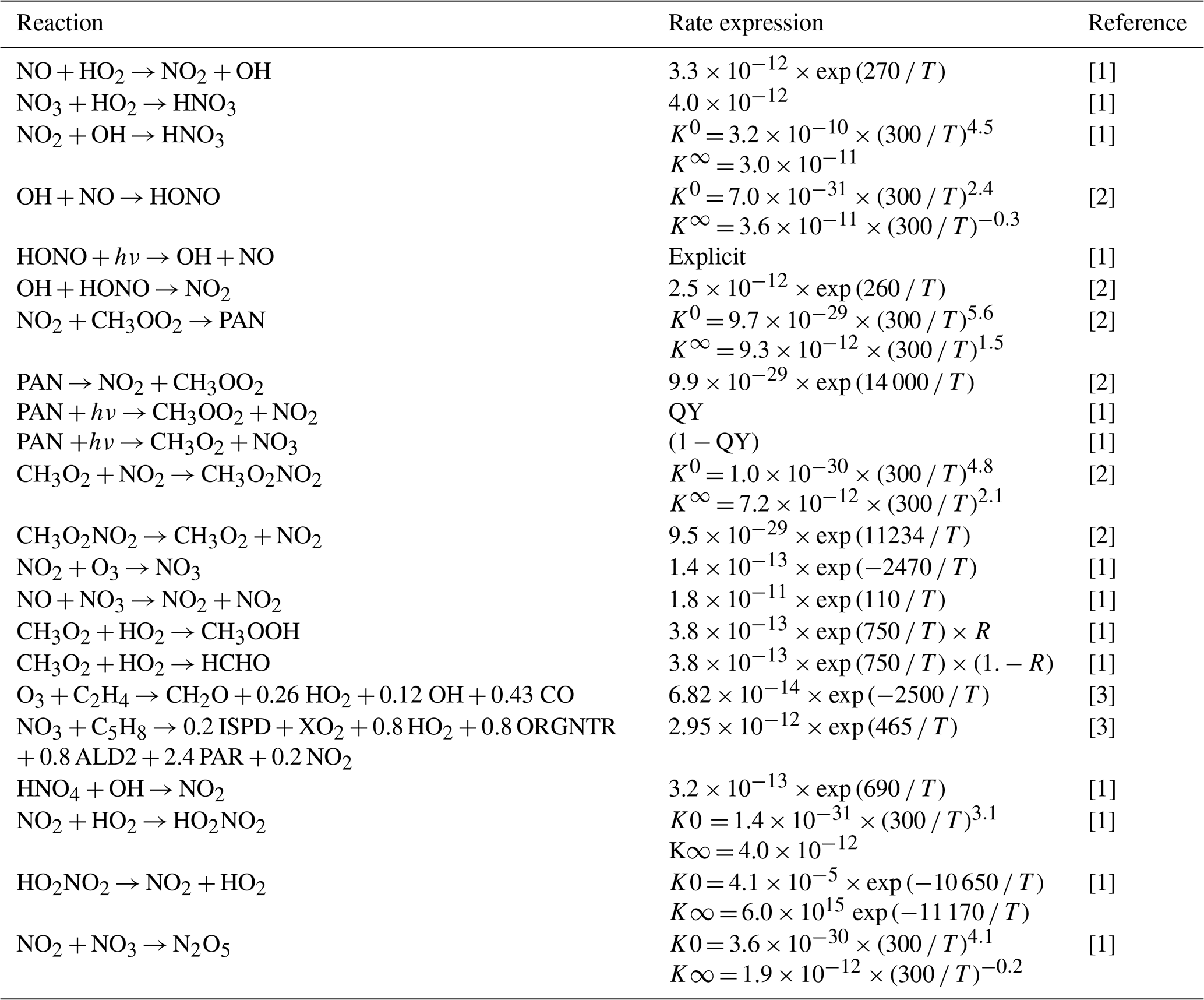
[1] Atkinson et al. (2004); updated according to http://iupac.pole-ether.fr (last access: 21 September 2021). [2] Burkholder et al. (2019). [3] Atkinson et al. (2006); updated according to http://iupac.pole-ether.fr (last access: 21 September 2021). The key to the abbreviations is as follows: T stands for temperature (^∘K), K⁰ stands for low-pressure limiting rate constant, K^∞ stands for high-pressure limiting rate constant, QY stands for quantum yield and R stands for product yield.

The updated rate data for NO_x chemistry and NO_y components are listed in Table 2 and are based on the updates tested in the chemistry transport model TM5 (Williams et al., 2017). One important update is the use of the new recommendation for the formation of HNO₃ (Möllner et al., 2010) that has been shown to have significant effects on the tropospheric O₃ burden (Søvde et al., 2011). HONO acts as an important source of OH and NO during the early morning from efficient photolytic destruction after nocturnal build-up (Stutz et al., 2004), whereas CH₃O₂NO₂ alters the NO_y chemistry in the free troposphere (Browne et al., 2011). Additionally, updates have also been made to the reaction data for O₃ + C₂H₄ and NO₃ + C₅H₈.

To date IFS(CBA) has only included a very simplistic parameterization for the oxidation of C₅H₈. To improve the realism of the product distribution from the oxidation of C₅H₈ by OH, we have developed a mechanism which is a hybrid of that developed by Stavrakou et al. (2010) and Lamarque et al. (2012). This new hybrid method includes the direct formation of glyoxal (CHOCHO), hydroxy-aldehydes (HPALD1, HPALD2), a peroxy product (ISOPOOH), glycolaldehyde (GLYALD), hydroxyacetone (HYAC) and methylglyoxal (CH₃COCHO). Explicit J values are calculated online for these products using the latest recommendations for absorption data, as for other species. Most of these intermediates are soluble with Henry solubility analogous to ALD2 except CHOCHO, where the approach of Ip et al. (2009) is used. We retain the intermediate isoprene oxidation product (ISPD), which is representative of both methyl vinyl ketone and methacrolein from previous versions of the scheme. Reaction rates in this mechanism have been updated following latest recommendations, as aligned with the mechanism described by Myriokefalitakis et al. (2020).

Validation of this updated component of the IFS(CBA) is beyond the scope of this study, but we have found that OH recycling increases over forested regions with high biogenic emission fluxes like that shown in Stavrakou et al. (2010), thus affecting atmospheric lifetime of individual trace gases for regions with high resident mixing ratios of C₅H₈. It should be noted that for O₃ and NO₃ we still adopt the original stoichiometry for the product distribution as in previous versions of IFS(CBA) (Huijnen et al., 2016). We provide details related to this extensive update in Table S1 in the Supplement.

To date aromatics were not explicitly treated in IFS(CBA) but rather as part of the generic paraffinic bond tracer PAR, which has now been updated. For this we follow the work of Karl et al. (2009), who describe the oxidation of the aromatic species toluene (TOL) and xylene (XYL), allowing a coupling to SOA formation. In addition, in our model version the product distributions and rate expressions for NO and HO₂ radical–radical reactions are taken from Myriokefalitakis et al. (2020). This links the aromatic species towards oxidant loss (O₃, OH, NO₃) and the production of CHOCHO/CH₃COCHO and allows the introduction of gas-phase precursors for SOA formation (SOG) from anthropogenic and BB sources. We provide details on the extension to the aromatic chemistry in IFS(CBA) in Table S2 in the Supplement.

Finally in Table S3 in the Supplement, we provide the rate data used for the oxidation of HCN and CH₃CN by OH. For CH₃CN we define a fraction (30 %) to be converted to HCN, following Li et al. (2009), but alternatively we prescribe it as a purely chemical sink process in the troposphere, on top of the loss at the surface due to ocean uptake. This allows it to be used as a tracer for selected air masses with the dominant emission sources being open burning fires (Li et al., 2000). Again, the validation of these new tracers is not relevant to this study therefore not presented here.

2.2 IFS(MOCAGE)

The IFS(MOCAGE) chemical scheme, hereafter called IFS(MOC), is a merge of reactions of the tropospheric RACM scheme (Stockwell et al., 1997) with the reactions relevant to the stratospheric chemistry of REPROBUS (Lefèvre et al., 1994, 1998). As in the IFS(CBA) implementation, IFS(MOC) uses a lumping approach for organic trace gas species. The IFS(MOC) initial tropospheric RACM chemistry scheme was extended and now includes the sulfur cycle in the troposphere, leading to the introduction of dimethyl sulfoxide (DMSO) and NH₃ gas species (Ménégoz et al., 2009; Guth et al., 2016). The current version of the IFS(MOC) chemistry scheme includes 123 species, including long-lived and short-lived species, family groups, a polar stratospheric clouds (PSC) tracer, 319 gas-phase thermal reactions, 56 photolysis reactions, and 14 heterogeneous reactions (9 for the stratosphere and 5 for the troposphere). The version adopted here is as that reported in Huijnen et al. (2019) with four major differences.

Firstly, in IFS(MOC), the formation of nitrate, ammonium and sulfate particles from NH₃, SO₂ and HNO₃ gaseous species is now activated in an analogous way to what is used in IFS(CBA). The nitrate and ammonium formation depends on resident sulfate concentrations (see Huijnen et al., 2019; Rémy et al., 2019). This primarily affects the modeled NH₃ and HNO₃ atmospheric burdens, but indirectly also affects the other trace gases through heterogeneous reactions.

Secondly, the formation of gaseous SOG from biogenic and anthropogenic and BB VOCs was implemented in IFS(MOC) following the simplified approach proposed by Spracklen et al. (2011). While biogenic sources (namely C₅H₈ and monoterpenes) are provided by the IFS(MOC) chemistry scheme, anthropogenic and BB emissions were scaled from the corresponding CO emissions. In this simplified approach, only two SOG low-volatility classes are considered, one for biogenic SOG and the other gathering both the anthropogenic and BB contributions. As in IFS(CBA), this SOG chemistry is coupled in IFS(MOC) with the aerosol module by solving the equilibrium of the partitioning between the gas and aerosol phases.

Recent developments in IFS(MOC) also include the modeling of the HCN and CH₃CN tracers with chemical loss being limited to oxidation by OH and photolysis in the stratosphere, using the same rate data as those used in IFS(CBA) (see Table S3) but with no products defined. As already stated for IFS(CBA), validation of these new tracers is not relevant to this study and therefore not presented here.

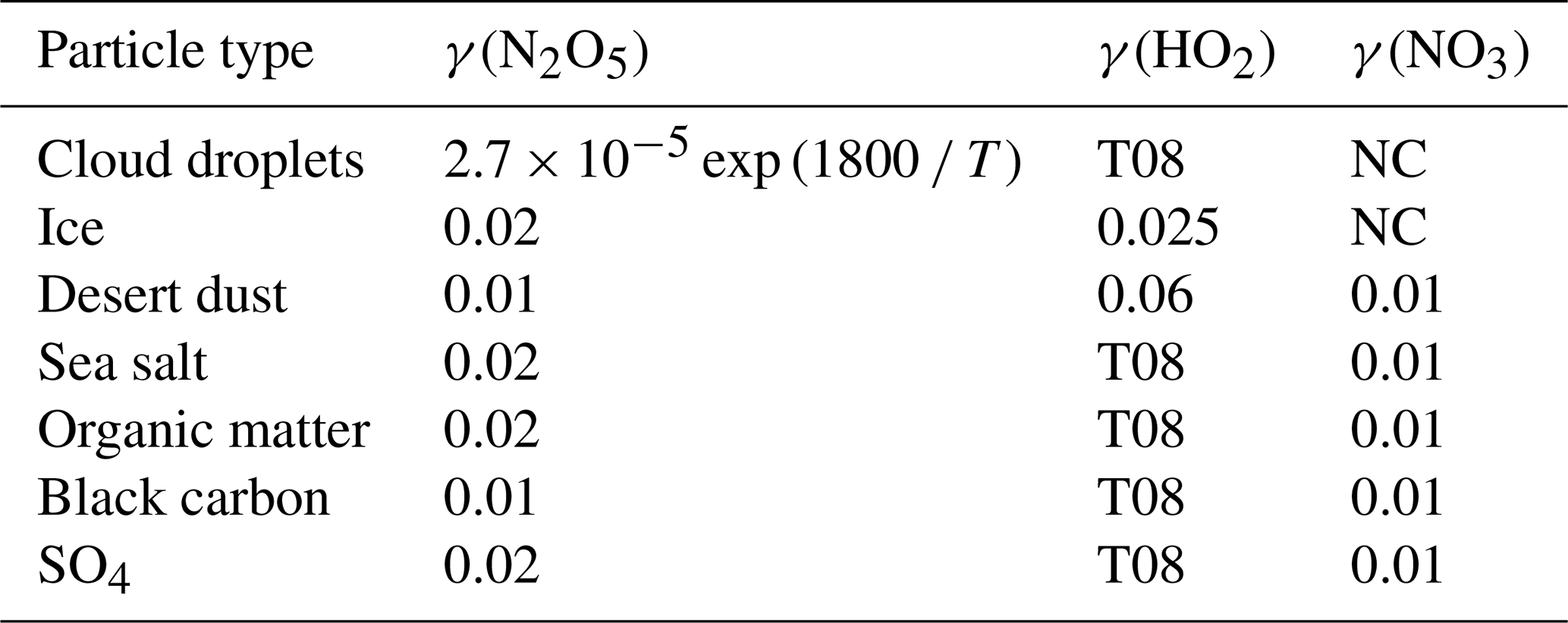
Last, the heterogeneous scavenging on aerosol, cloud droplets and ice particles for N₂O₅, HO₂ and NO₃ has been fully updated and made consistent with the IFS(CBA) configuration, which is based on the latest recommendations. For the sake of simplicity, the heterogeneous reaction probabilities (γ) are for most surfaces considered constant, as summarized in Table 3. The reaction probability γ(HO₂) is computed following Thornton et al. (2008), taking the role of pH and partition between the gaseous HO₂ and the dissociated form (${\mathrm{O}}_{\mathrm{2}}^{-}$) into account, adopting a constant pH of 5.5. It follows the description given in Huijnen et al. (2014), where further details are given.

Table 3 Heterogeneous γ values used for prescribing conversion rates on atmospheric cloud droplets, ice and aerosols. “T08” refers to Thornton et al. (2008) and “NC” indicates not considered.

2.3 IFS(MOZART)

The IFS(MOZART), hereafter referred to as IFS(MOZ), is based on the Model of Ozone and Related chemical Tracers (MOZART) mechanism (Kinnison et al., 2007; Emmons et al., 2010) and includes additional species and reactions from the Community Atmosphere Model with interactive chemistry, referred to as CAM4-chem, a component of the Community Earth System Model (CESM) (Tilmes et al., 2016).

The IFS(MOZ) version used here is comparable to that described and evaluated in Huijnen et al. (2019) with a few additional updates. The TOL lumped aromatic used in the previous version has been replaced by the separate species benzene, toluene and xylene, allowing for accounting for their different lifetimes and oxidation products. The current version also includes formic acid (HCOOH) and ethyne (C₂H₂) and their oxidation products. The reaction rates have been updated to follow the recommendations from IUPAC (http://iupac.pole-ether.fr, last access: 21 September 2021) or JPL-2015 (Burkholder et al., 2019). Updates have also been introduced to the photolysis look-up table, which includes explicit calculations of photolysis frequencies for most of the IFS(MOZ) species. The heterogeneous chemistry in the troposphere is implemented according to the corresponding module from IFS(CBA) to account for heterogeneous uptake of N₂O₅, HO₂ and NO₃ on aerosols as described in the previous section. However, the heterogeneous uptake on ice and cloud droplets is currently not included in IFS(MOZ).

Finally, nitrate, ammonium and sulfate particle formation have been introduced in IFS(MOZ) analogous to IFS(CBA) and IFS(MOC) (Rémy et al., 2019), involving gaseous SO₂, NH₃ and HNO₃, as described above.

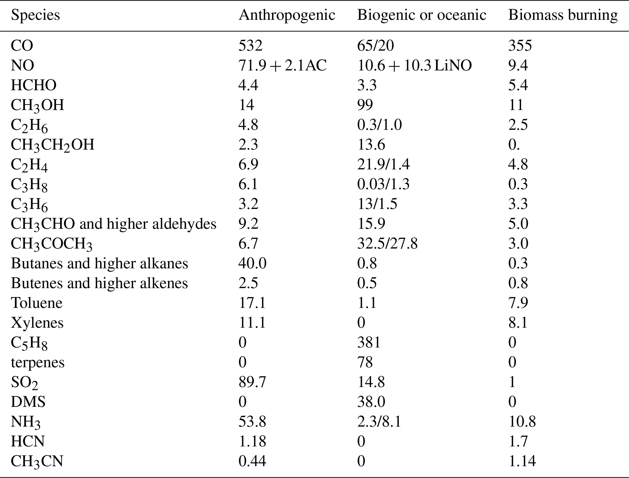
Table 4 Global annual mean emissions for 2014 as adopted in current IFS(CBA) model simulations [Tg species yr⁻¹]. No direct emissions of HONO are included. For NO, the aircraft (AC) and lightning NO_x (LiNO) emissions are also given as anthropogenic and biogenic contributions, respectively.

2.4 Setup of model simulations

The model simulations using the new developments described above have been performed with IFS cycle 47r1. The simulations were run using 137 vertical levels and a horizontal resolution of T_L255​​​​​​​, corresponding to ∼ 0.7^∘ × 0.7^∘, excluding data assimilation of atmospheric composition. A model top of 1 Pa is defined for these vertical grid settings.

The simulations evaluated here are executed as a series of 24 h hindcasts, initialized daily at 00:00 UTC from ERA5 meteorology (Hersbach et al., 2020). A 30 min time step was used. A 4-month spin-up period is employed to allow the system to reach chemical equilibrium during September to December 2013, after which an 18-month simulation was performed to allow the use of wintertime measurements for deriving some seasonality in the analysis. To limit the volume of data, outputs of 3D chemical fields are archived at a 3-hourly time interval and subsequently interpolated to the relevant time stamp of each measurement. The experiments are archived with experiment identifiers b28w for IFS(CBA), b0ov for IFS(MOC) and b0yw for IFS(MOZ).

For comparison, the CAMS Reanalysis (CAMSRA), which includes data assimilation of O₃, CO, NO₂ and aerosol optical depth (AOD), uses IFS cycle 42r1. CAMSRA was run at the same horizontal resolution (T_L255) as the experiments presented here, but with only 60 model levels and a model top of 0.1 hPa (Inness et al., 2019). Different emission estimates were also employed for the CAMSRA dataset, meaning that interpretation of differences need to be done with care.

The emissions adopted in this configuration are taken from CAMS_GLOB_ANT v4.2-R1.1 (Granier et al., 2019; https://eccad.aeris-data.fr/, last access: 25 May 2022), which is a modification of the v4.2 global anthropogenic emission dataset used operationally in CAMS, with reduced emission strength over China. Biogenic emissions are taken from the CAMS_GLOB_BIO v1.1 dataset (Doubalova et al., 2018; http://eccad.aeris-data.fr/, last access: 25 May 2022), and BB emissions are taken from GFAS v1.2 (Kaiser et al., 2012), which are applied using the methodology as described in Ye et al. (2021). As GFAS does not provide separate estimates for HCN and CH₃CN emissions, we scale them from the CO emissions. Other (oceanic, natural) emissions are taken from the standard configuration in IFS (see Huijnen et al., 2019).

Apart from BB and SO₂, all emissions are applied in the lowest model level. Information on emission totals used in the simulations is given in Table 4 for IFS(CBA). This corresponds essentially to the emissions as adopted in IFS(MOZ) and IFS(MOC), with small variations in the partitioning of some of the lumped VOCs, such as the higher alkanes, alkenes and aldehydes, as well as the aromatics. When comparing emission totals with those used in Huijnen et al. (2019), the main differences are 10 % lower primary emissions for anthropogenic CO and SO₂, a 20 % increase in anthropogenic NH₃, approximately equal NO_x emissions, and most importantly a 20 % reduction in C₅H₈. The variability in the emission estimates compared to previous studies are due to both the use of different data in the derivation of fluxes and trends in the annual emission estimates (2014 versus 2019).

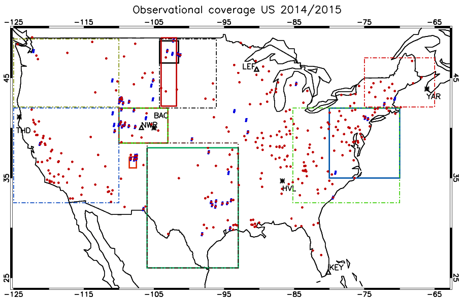
Figure 1 The location of surface measurement stations and areas sampled during the numerous aircraft campaigns. The ozonesonde locations are shown as ^∗, and the GFDL surface sites are shown as Δ. Key to airshed definitions: North Dakota (May 2014, full black), New Mexico (June 2014, full red), Colorado (July–August 2014 and March–April 2015, light green), Eastern Coast (February–March 2015, full dark blue) and south central US (April 2015, full dark green). The areas outlined by the dashed and dotted borders are associated with the regions for which the AirNow observations are analyzed, with the reader being referred to Table 6. The individual stations for the AirNow network are shown as red dots (O₃), and blue dots (NO₂) are used for rural stations only.

3 Observations

In this section we provide an overview of all the observational data used to evaluate the performance of the three IFS versions for the years 2014 and 2015. Figure 1 shows the location of all the measurement stations and regions covered by the aircraft campaigns utilized for assessing the different versions of the IFS.

3.1 Surface flasks and soundings for CO and O₃

For tropospheric O₃ we use seasonal composites from four individual sites from the World Ozone and Ultraviolet Radiation Data Center (WOUDC; http://woudc.org, last access: 25 May 2022​​​​​​​), namely Yarmouth (43.9^∘ N, 66.0^∘ W), Boulder (40.0^∘ N, 105.0^∘ W), Trinidad Head (41.1^∘ N, 124.2^∘ W) and Huntsville (34.7^∘ N, 86.7^∘ W). Although Yarmouth is not in the US it provides a good proxy for New England air quality. Each station samples a different region, allowing the assessment of performance at continental scale, with an associated error of around ± 10 % (Komhyr et al., 1995; Steinbrecht et al., 1998). The location of each station is shown in Fig. 1.

For evaluating the surface mixing ratios of O₃, we compare monthly mean mixing ratios against corresponding values taken from three measurement sites at Trinidad Head (41.1^∘ N, 124.2^∘ W), Boulder (40.0^∘ N, 105.0^∘ W) and Niwot Ridge (40.1^∘ N, 106.5^∘ W), which are part of the Geophysical Fluid Dynamics Laboratory (GFDL) monitoring network. These observations are taken from the long-term measurement network maintained by the NOAA Earth System Laboratories (ESRL) Global Monitoring Laboratory. Correspondingly, for CO we use surface observations from the ESRL stations Park Falls (LEF, 45.9^∘ N, 90.4^∘ W), Niwot Ridge (NWR, 40.1^∘ N, 105.6^∘ W) and Key West (KEY, 25.6^∘ N, 80.2^∘ W). These observations have an associated uncertainty of between 1 and 3 ppb (Novelli et al., 2003).

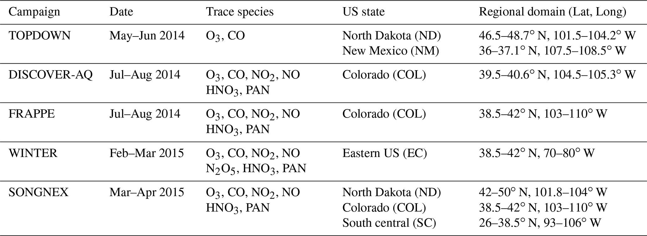
Table 5 Details of the various aircraft measurement campaigns in 2014/2015 used in this study.

3.2 Aircraft observations

Figure 1 also shows the predefined airsheds used to evaluate the lower troposphere (LT) over various regions across the US during 2014 and 2015. There is a paucity of aircraft data over the western part of the US, as most aircraft campaigns focus on industrial regions or those influenced by energy production techniques such as fracking for the chosen evaluation year. Data from the following campaigns are used.

• TOPDOWN (May/June 2014): springtime campaign focusing on emissions from rural fracking sites located in North Dakota and New Mexico: (https://csl.noaa.gov/groups/csl7/measurements/2014topdown/; last access: 28 September 2021).

• Front Range Air Pollution and Photochemistry Éxperiment (FRAPPÉ)/Deriving Information on Surface conditions from Column and Vertically Resolved Observations Relevant to Air Quality (DISCOVER-AQ) (July–August 2014): summer campaign investigating O₃ exceedances due to regional VOC and NO_x emissions in Colorado (Dingle et al., 2016; McDuffie et al., 2016; Flocke et al., 2019). More details related to DISCOVER-AQ can be found at https://www.nasa.gov/larc/2014-discoveraq-campaign/ (last access: 28 September 2021).

• Wintertime INvestigation of Transport, Emissions, and Reactivity (WINTER) (February–March 2015): winter campaign over the US East Coast to investigate O₃ and NO_x chemistry over Virginia and North Carolina (McDuffie et al., 2018; Jaeglé et al., 2018).

• Studying the Atmospheric Effects of Changing Energy Use in the US at the Nexus of Air Quality and Climate Change (SONGNEX) (March–April 2015): spring study on effects of shale and natural gas extraction on air quality across the US (https://csl.noaa.gov/projects/songnex/; last access: 28 September 2021, Peischl et al., 2018; Koss et al., 2017).

The aircraft campaigns, whose regional coverage and trace species are given in Table 5, are either segregated into different legs for different US states or sample air over a wide area for different days. In the latter case we segregate spatially during the analysis to provide more regional coverage. Lower limits for the trace gases NO₂ and NO_y are placed on the observations as determined by the detection limits of the instrumentation of 40 ppt as stipulated in the data files. For NO₂, HNO₃ and PAN dual measurements are available from different instruments, which are merged to increase the available sampling frequency. For N₂O₅, a maximum of 1.3 ppb is placed on the observations for the comparisons presented to avoid spurious values.

We interpolate 3-hourly data from the model simulations using the time, geolocation and pressure of the observations, then average over predefined pressure bins of around 50 hPa ensuring that there are a sufficient number of observations per bin. We also calculate mean bias statistics for the LT using selected pressure tops of 815 (COL), 900 (EC), 880 (ND) and 965 hPa (SC) accounting for the variable orography and to include enough points as to be statistically robust. The resulting mean bias values and associated standard deviation from the mean are presented in Tables S4 and S5 in the Supplement for O₃ and CO and Tables S7 and S8 in the Supplement for NO₂ and NO.

Table 6 Details of the various regions defined for assessing simulated surface concentrations for O₃, CO and NO₂ using data from the AirNow measurement network. The total number of individual stations for each respective species is given in the rightmost column.

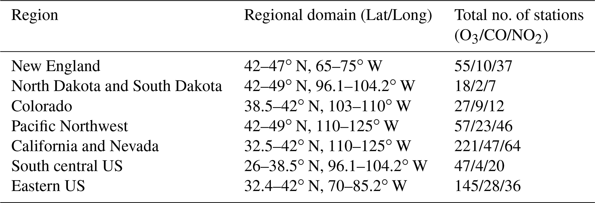
3.3 Surface air quality networks for O₃, CO and NO₂

For evaluating surface concentrations from the model we exploit observations of O₃, CO and NO₂ from the AirNow (http://www.airnow.gov, last access: 28 September 2021) air quality observations network. Within the AirNow centralized system, hourly measurements of O₃, NO₂, CO, PM_2.5 and PM₁₀ are collected from measurement locations across the US, submitted by state or local monitoring agencies and made available in near real time after preliminary data quality assessments have been performed. Here we use data collected over the 2014 period for the designated domains, which includes 570, 222 and 123 monitoring stations for O₃, NO₂ and CO, respectively. The list and definition of each of the sub-domains over which statistical scores are provided is given in Table 6, together with the number of stations used in the current study. Each station is designated a classification being either urban, suburban or rural depending on the location of each station in order to differentiate between clean and polluted sampling locations. Only clean background comparisons are shown due to the difficulty of global models representing small-scale gradients in concentrations typically found near roads and industrial point sources. We use version v1.0.3 of the evaltools statistical package available online (https://opensource.umr-cnrm.fr/projects/evaltools, last access: 20 December 2021).

Additionally, a filtering procedure was applied to the data before computing the daily mean values to remove stations where the time series displayed more than 50 % of identical values, denoting a failure in the measurement sensor. Moreover, for CO the observational values < 50 and > 1200 µg m⁻³ were filtered out at the rural stations to avoid spurious instrumental effects. The 3-hourly model output was spatially interpolated from the model grid to the stations network. Time series of daily mean composites were then obtained by computing the daily mean values across stations with identical station classification for each domain, using both the observed and simulated data during 2014, providing a spatial mean of the concentrations. For brevity we do not show any comparisons for 2015. Details on the accuracy of the instrumentation used across the network can be found in Williams et al. (2014).

3.4 Surface network for HNO₃

Finally, in order to evaluate the near-surface concentrations of HNO₃, we use the near-surface mixing ratios taken from the Clean Air Status and Trends Network (CASTNET; https://www.epa.gov/castnet, last access: 30 September 2021), which provides filter pack measurements at weekly intervals for 87 individual sites located in rural locations away from strong NO_x emission sources. This dataset is therefore a measure of the chemical processing that occurs in transported air masses at regional scale. The inferred mixing ratios result from the application of the multilayer model (Finkelstein et al., 2000) to these samples, which uses site-specific meteorological parameters to determine deposition values. We only use the near-surface mixing ratios here, as assessing the wet deposition component of the chemical modules is beyond the scope of this paper and more associated with the aerosol modules applied in IFS. For brevity, we aggregate and compare seasonal mean values of the mixing ratios as interpolated from the model data using the location and height of each station for correct interpolation. It should be noted that from an intercomparison of gaseous HNO₃ values, CASTNET data were found to be typically lower than those of other measurement networks (Lavery et al., 2009). However, CASTNET data composites are typically used for assessing the performance of deposition processes in global transport models and are from an established dataset.

Figure 2 The horizontal seasonal mean for tropospheric O₃ below 1 km over the US domain for JJA 2014 (top) and DJF 2014/2015 (bottom).

Figure 3 Seasonal O₃ sonde comparisons for seasons JJA (top) and DJF (bottom) for the lower troposphere. Stations shown are Trinidad Head, Boulder, Huntsville and Yarmouth, which are situated across the US and Canada. The observational composites are shown in black, with the color key provided in the top-left panel. The geolocation of each site is given in the title of each panel, and the number of observations used is given at the bottom right of each panel. Please note that the scales on the x and y axes vary with respect to station.

4 Results

4.1 Tropospheric O₃

The seasonal horizontal mean distribution of tropospheric O₃ in IFS(CBA) and the associated relative differences for the IFS(MOC) and IFS(MOZ) against IFS(CBA) are shown for seasons June–July–August (JJA) and December–January–February (DJF) over the US in Fig. 2. We select all levels below 1 km for calculating the seasonal means, which allows a direct comparison for coastlines and elevated regions (namely Colorado). For DJF we choose 2014–2015 data to be fully conversant with the validation of the vertical profiles (see below) and when the system has achieved chemical equilibrium for longer-lived species.

For JJA, the seasonal distribution shows higher mixing ratios exceeding 65 ppb at both the US East Coast and US West Coast driven by regional NO_x and VOC emissions. There is a minimum in central rural regions around Kansas and Nebraska and North Dakota and South Dakota, with a variability of between 35 and 45 ppb in IFS(CBA). Examining regional differences shows that when enhancements in (near-)surface O₃ typically occur, both IFS(MOC) and IFS(MOZ) show a ± 5 % variability with respect to IFS(CBA), with maximal differences on the US East Coast of +4 %–6 %. IFS(MOZ) exhibits a decrease in mixing ratios of between 5 and 10 ppb due to the transport of cleaner air masses compared with IFS(CBA), especially for the ocean off the Pacific Northwest. During DJF the model shows a weak west–east gradient with a lower range of mixing ratios of 30–50 ppb. For DJF, the range of the differences is substantially higher (∼ 8 %–35 %) than for JJA, with IFS(MOZ) having a significant excess in O₃ towards the US East Coast with respect to IFS(CBA). Therefore, under identical NO_x emissions, the O₃ production efficiency via the reactive NO_x cycle is highest for IFS(MOZ), indicating a lower rate of termination towards NO_y (See Sect. 6). This subsequently increases mixing ratios of the OH from the primary production term involving photolysis of O₃ in the presence of water vapor (H₂O) (see Fig. S1 in the Supplement).

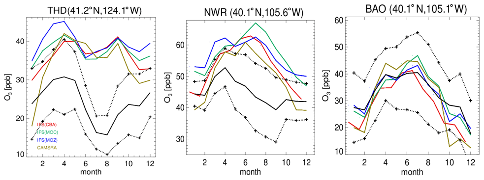
Figure 4 Comparisons of surface O₃ measurements for 2014 for the three GFDL stations situated in the US, namely THD, NWR and BAO. The observational means and the corresponding 1σ variability are shown as the solid and dashed black lines, respectively.

Evaluations against seasonal ozonesonde composites of all available measurements for JJA and DJF located across the US and Canada for the lower troposphere, as shown in Fig. 3, also exhibit a signature of the seasonal mean differences as discussed for Fig. 2. For JJA there are positive biases near the surface for Yarmouth (east coast), whereas for Trinidad Head (west coast) biases are smaller, and thus the agreement is more favorable. The highest bias, between 10 and 20 ppb, is shown for Huntsville in Alabama, where the station is affected by the transported plumes from nearby cities (Newchurch et al., 2003). In general, the correct profile shape is captured for most sites, except for Trinidad Head where a steep gradient is observed. For DJF, there is more variability across the chemical modules, where IFS(MOZ) exhibits the highest mixing ratios towards the east coast, leading to a positive bias of 15 ppb at Yarmouth. Again, profile shapes are captured well across the stations.

In Fig. 4 the corresponding annual cycle in monthly mean mixing ratios for surface O₃ at the three continuous measurement sites available in the US are shown, with Boulder Atmospheric Observatory (BAO) and Trinidad Head (THD) being co-located in the vicinity of the sonde measurements. For THD, which is situated at the outermost US West Coast, the observed monthly mean mixing ratios are very low. This indicates the absence of significant local NO_x emissions, which are therefore being influenced by land–sea air movements, allowing the sampling of clean Pacific air (Oltmans et al., 2008). For most months in THD and Niwot Ridge (NWR), there is a bias of up to 100 % across the different chemical modules, with a more muted amplitude in monthly variability than observed, indicating difficulties of the global model configuration towards capturing the correct seasonal cycle. Apart from model resolution effects, the transport of air from out of the US could be too efficient, as described by the transport processes, or the production and loss over the ocean surface may not be in the correct equilibrium. Comparing IFS(CBA) and CAMSRA there has been an increase of between 2 and 10 ppb in surface O₃ mixing ratios, increasing the simulated biases somewhat.

Even though the stations BAO and NWR are relatively close together, there is a diverse shape in the annual cycle showing the influence of regional NO_x chemistry, topography, meteorology and station height (1.5 versus 2.9 $\mathrm{km}\mathrm{a}.\mathrm{s}.\mathrm{l}.$). Transport of pollutants from the Denver region affects O₃ mixing ratios at NWR (Chin et al., 1994; McDuffie et al., 2016), and it is thus representative of a chemically aged air mass. The BAO site is also influenced by anthropogenic emissions with measurements sampling the boundary layer (Gilman et al., 2013; McDuffie et al., 2016). At BAO the annual cycle and maximal mixing ratios are captured well across simulations. For NWR, which samples air at an elevated site, there is no strong annual cycle in the measurements, whereas for the CAMSRA and the mini-ensemble a maximum occurs during JJA with a bias of between ∼ 50 % and 70 %.

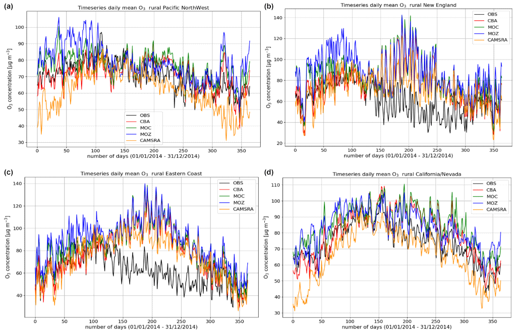
Figure 5 Comparisons of the daily mean variability surface O₃ for 2014 against regional composites assembled from measurement sites for rural locations contributing to the AirNow network. Regions shown (a to d) are the Pacific Northwest, New England, eastern US, and California and Nevada.

Table 7 Annual mean biases and Pearson's R values for the comparison of surface O₃ versus AirNow data for 2014.

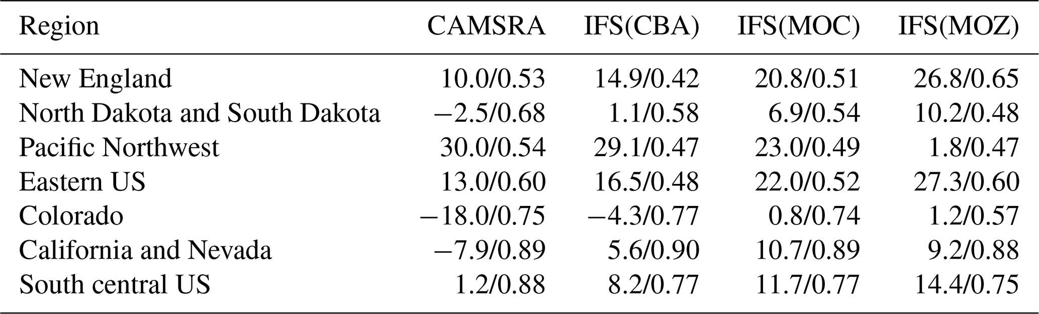
The variability in the daily mean values in surface O₃ simulated by the chemistry modules are evaluated against selected regional composites of measurements taken from the AirNow network assembled for 2014; see Fig. 5. Comparisons are performed for the regions defined in Table 6 (Sect. 3), where only those stations that are classified as rural (i.e., away from urban conurbations) are used. The associated annual mean biases (AMB) and Pearson's R coefficients are provided in Table 6. Model performance is regionally dependent, with larger biases for regions exhibiting strong seasonality on the meteorology and the length of day (e.g., California and Nevada). During the first few months of 2014, a significant mean positive bias exists for more northerly regions across the chemical modules, with IFS(CBA) biases up to 20 µg m⁻³ and IFS(MOZ) biases as high as 40–60 µg m⁻³. For CAMSRA, the corresponding mean biases are negative up to 40 µg m⁻³ (Pacific Northwest). The corresponding AMB values show that positive biases exist for most regions, except for Colorado. The degree of correlation is variable, being only moderately correlated for, e.g., North Dakota and South Dakota (R  = 0.48–0.68), while being highly correlated for, e.g., California and Nevada (R = 0.77–0.88). When comparing regions, small biases (of a few µg m⁻³) and higher correlation are found for the south of the US.

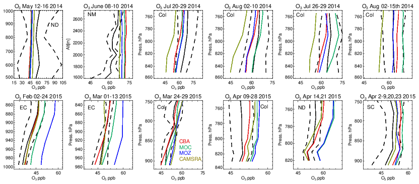
Figure 6 Comparisons of lower tropospheric O₃ profiles for 2014/2015 against composites of aircraft measurements for the regional domains shown in Fig. 1. The 1σ standard deviation of the mean for the observational values are shown as the dashed line. Campaigns shown (top left to bottom right) are TOPDOWN, DISCOVER-AQ, FRAPPE, WINTER and SONGNEX.

Vertical profiles in the LT from both the aircraft and simulations across the various US regions are shown in Fig. 6, with the boundaries of various regions given in Fig. 1 and Table 5. The corresponding mean bias statistics are documented in Table S4. The shallow to moderate gradients in LT O₃ seen in the observations are simulated relatively well across the various chemistry modules, albeit with changing variability and bias across the regions. For summertime, most comparisons are for the Colorado region over Denver and the surrounding area, where O₃ production is heavily influenced by oil and natural gas production and industry (Cheadle et al., 2017), exhibiting mean values of 60–65 ppb for the (near-)surface. During July the region experienced a strong cyclonic front, whereas in August non-cyclonic conditions occurred (Vu et al., 2016) resulting in different transport dynamics for each period, although little impact is seen in the mean value. Here, the monthly negative biases are of the order of −2 to −10 ppb, indicating too low regional NO_x emissions (see Table S3) and showing that the persistent positive bias seen at more globally remote regions (Huijnen et al., 2019) does not occur during summertime for more polluted urban regions. For CAMSRA, more significant negative biases exist of between 10 and 15 ppb.

The evaluation during boreal wintertime over the US East Coast, which has lower observed O₃ mixing ratios of 38–45 ppb, reveals there is more divergence across the chemistry modules under these conditions, with IFS(MOZ) showing high positive biases of ∼ 10 ppb, whereas IFS(CBA) captures the observational mean profile well within a few parts per billion. This leads to high oxidative capacity for IFS(MOZ), which has a subsequent impact on tropospheric CO (see the next section). This evaluation highlights differences in model performance in the lower troposphere compared to those presented for the surface O₃ analysis. In that vertical mixing has occurred means that this analysis is not subject to the representation of locational issues with measurement sites (local emission sources such as roads, the effects of building on transport, etc.). For springtime over Colorado, mixing ratios are somewhat lower than summertime (∼ 50 ppb), where IFS(CBA) shows a small negative bias of a few parts per billion, with the positive bias for IFS(MOZ) persisting (5 ppb). For the south central US region, a positive bias of 5 ppb occurs across chemistry modules, with the CAMSRA dataset having similar biases throughout regions during springtime.

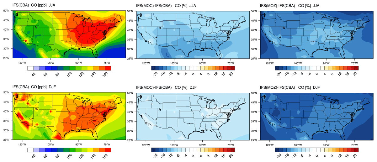
Figure 7 The horizontal mean cross section of CO below 1 km over the US domain for JJA 2014 (top) and DJF (2014/2015).

Figure 8 Comparisons of monthly mean surface CO mixing ratios at three separate surface measurement sites across the US. The observational monthly means with the variability are shown in black.

4.2 Tropospheric CO

The corresponding US continental distribution for seasonal mean tropospheric CO for IFS(CBA) for JJA and DJF are shown in the top and bottom left panels of Fig. 7, respectively. A distinct east-west gradient exists with ∼ 50 % higher mixing ratios towards the East coast reaching ∼ 150–160 ppb. No distinct burning regions are visible towards the west coast associated with comparatively low BB activity for 2014 in the US (Petetin et al., 2018). The two other chemistry modules have consistently lower mixing ratios under identical primary CO emissions, indicating differences in the chemical production rate from the oxidation of formaldehyde (CH₂O) and higher VOCs, combined with differences in the chemical lifetimes because of OH variability (Huijnen et al., 2019). For IFS(MOZ) we diagnose a comparatively low tropospheric CO burden associated with a fast oxidation rate due to higher mixing ratios of OH in the LT of between 20 % and 50 %; see Fig. S1). This is directly associated with the higher O₃ (see Fig. 2) in IFS(MOZ). For DJF, a much shallower continental gradient exists with average mean mixing ratios of between 100–120 ppb, with IFS(MOC) and IFS(MOZ) again exhibiting negative differences compared to IFS(CBA). The distribution of CO for this season in IFS(CBA) shows signatures of increased pollution visible over large urban centers in, e.g., California, Washington state and New York state, in line with figures presented for LT O₃ related to regional NO_x emissions (see next section).

The seasonal cycle in surface CO mixing ratios is compared against monthly mean composites from the ESRL observational network. The seasonal cycle is somewhat determined by the regional CO emissions, as exemplified by the increase observed for July at Park Falls (LEF), which is possibly due to local BB events for this year (Blunden and Arndt, 2015). A signature exists at NWR from the chemical processing of polluted air masses from the Denver region during summertime (McDuffie et al., 2016), where all members show similar positive biases and sampling accounts for the elevated station height. For Key West (KEY), the seasonal cycle is representative of the outflow from the continental US, where all members capture the monthly variability quite well. For many of the individual months, IFS(CBA) shows a mild improvement when compared to the CAMSRA dataset, which shows a persistent positive bias especially during boreal wintertime. IFS(MOZ) exhibits the largest negative bias across stations in line with the lower mixing ratios shown in Fig. 7. In some instances, biases are of the order of 100 %, especially for winter months where OH is typically lower (see Fig. S1) and pollution is less mixed into the free troposphere.

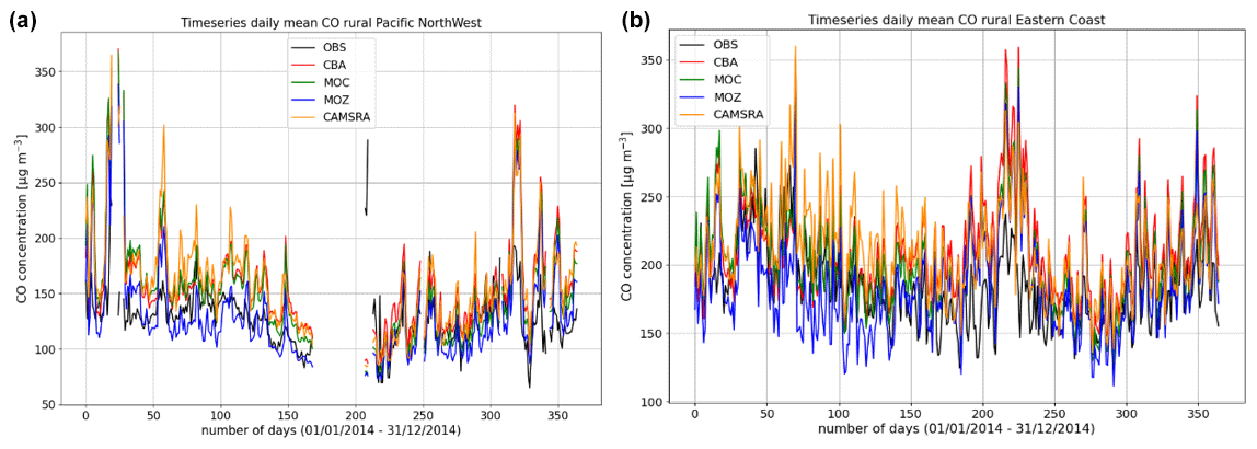
Figure 9 Comparisons of the daily variability of surface CO for 2014 against regional composites assembled from measurement sites participating in the AirNow network. Regions shown are the (a) Pacific Northwest and (b) US East Coast as determined by the number of available measurements for the rural classification.

Table 8 Annual mean biases and Pearson's R values for the comparison of simulations versus AirNow data. Unlike O₃, most regions do not have enough CO stations designated as rural for a valid comparison.

More extended regional composites for surface CO have been assembled using data available from the AirNow measurement network, with two regional comparisons of the daily variability in surface CO at rural locations for the Pacific Northwest and eastern US being shown in Fig. 9. The number of stations used for the comparison is lower than that used for the other species as limited by data availability (see Table 6), and for some regions an insufficient number of rural classified stations exist, meaning that no comparison is possible. No significant annual cycle is present for the domains shown. For boreal wintertime, again IFS(MOZ) (IFS(CBA)) exhibits the largest (smallest) negative bias as seen for the ESRL comparisons (Fig. 8 above). Table 8 provides the corresponding AMB and Pearson's R values, where generally there are positive biases across regions apart from IFS(MOZ) for the Pacific Northwest. There is a moderate correlation for the Pacific Northwest and only a weak correlation for the eastern US, which is influenced more by anthropogenic emissions.

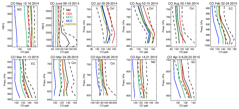
Figure 10 The same as Fig. 6 but for tropospheric CO. Campaigns shown (top left to bottom right) are TOPDOWN, DISCOVER-AQ, FRAPPE, WINTER and SONGNEX.

Tropospheric CO profiles in the LT are compared against the corresponding aircraft composites across the various campaigns in Fig. 10. As for O₃, the shape of the vertical profiles is captured well (i.e., gradients and the inflection between the boundary layer and free troposphere) with a significant variability in mixing ratios across the ensemble as shown in the seasonal mean comparisons in Fig. 7. For NM the convex bulge seen in the LT is not captured well by the ensemble with high negative biases (cf. Table S5), most probably due to missing emissions from energy production (fracking) which was the focus of this measurement campaign (Peischl et al., 2018). High negative biases of 35–60 ppb occur for June 2014, showing a significant underestimation in either primary emissions or VOC precursors (no measurements available) for this region. For boreal summertime over Colorado, mean values between 100 and 130 ppb exist, where IFS(CBA) exhibits positive biases of 5–20 ppb (cf. Table S5). Comparing IFS(CBA) against CAMSRA shows there is only a modest difference in CO, with slight increases in the associated negative biases. Biases presented in Table S2 shows that, assuming comparable data quality, the influence of local effects related to positioning and selection of stations can result in more extreme biases. For the aircraft composites surface effects are not so important where mixing in the boundary layer provides a more homogenized value. For both wintertime and springtime the higher observed mean values of 130–175 ppb are not captured by the mini-ensemble, with underestimates of 10–40 ppb depending on the month and region, suggesting too low primary emissions over a wide area, with CAMSRA exhibiting the lowest biases.

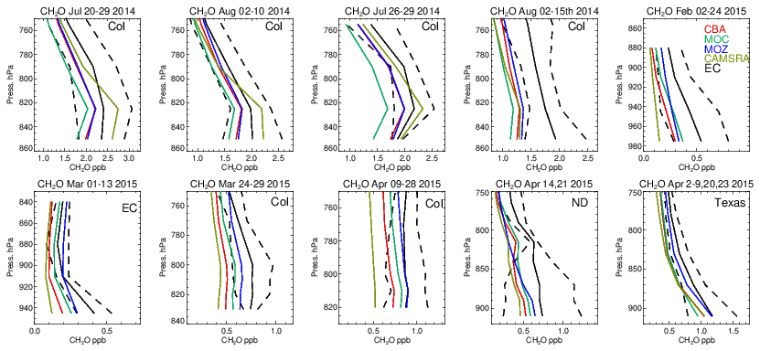
Figure 11 Comparisons of lower-tropospheric CH₂O profiles for 2014/2015 against composites of aircraft measurements for the regional domains shown in Fig. 1. Campaigns shown (top left to bottom right) are DISCOVER-AQ, FRAPPE, WINTER and SONGNEX.

One dominant precursor for the chemical production of CO is the oxidation of CH₂O (e.g., Zeng et al., 2015). The corresponding comparisons of CH₂O for all chemical modules are shown in Fig. 11, with associated biases in Table S6 in the Supplement. In the LT during boreal summertime conditions, C₅H₈ acts as a dominant source of CH₂O resulting in high mixing ratios over Colorado of 1.7–2.5 ppb. Generally, all chemical modules exhibit negative biases, except for the CAMSRA dataset, associated with the higher C₅H₈ emissions that are applied (MEGAN-MACC; Sindelarova et al., 2014). There is a higher variability associated with the simulations than that observed showing the sensitivity towards both photolysis and dissolution into cloud droplets, which introduces complications in short-term (daily) modeling of CH₂O. Note that the higher CH₂O in CAMSRA is not directly correlated with higher CO due to effective CO data assimilation being applied.

During wintertime biogenic fluxes are low due to the seasonality in biogenic activity, thus CO comparisons shown for February and March can be considered to be representative of the background supplemented with regional anthropogenic emission sources, considering the tropospheric lifetime of 1–2 months (e.g., Williams et al., 2017). This results in the resident mean CH₂O value being only a quarter of those seen for boreal summertime over Colorado. Under these conditions, the relative negative biases for CH₂O increase to ∼ 40 %–60 % across the chemical modules, with IFS(CBA) having twice the negative bias compared to IFS(MOZ). Given the low biogenic precursors, the overall negative bias suggests a deficit in the chemical production term of CH₂O likely from the limited oxidation of other VOCs or peroxy radical termination reactions, combined with missing direct HCHO emissions (Green et al., 2021). For springtime, relative biases are higher than in boreal summertime for Colorado across chemical modules, with values for the southern US being simulated with low relative biases of around 20 %.

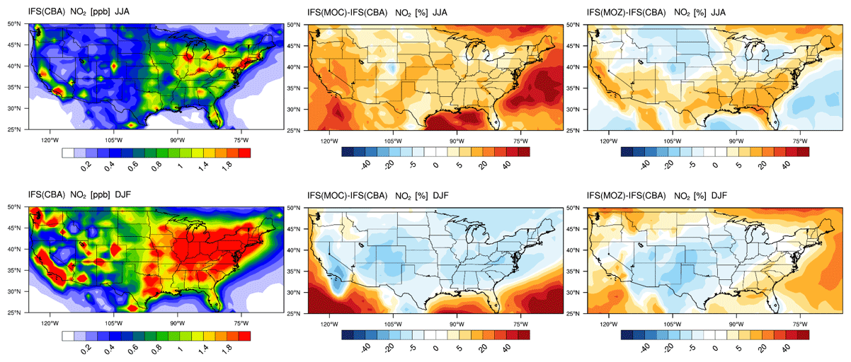
Figure 12 The horizontal mean cross section of NO₂ below 1 km over the US domain for JJA 2014 (top) and DJF (2014/2015).

4.3 Tropospheric NO₂

The seasonal horizontal mean distributions of tropospheric NO₂ for IFS(CBA) for JJA and DJF are shown in the left panels of Fig. 12. The large spatial variability in NO_x emissions can be clearly seen, resulting in much more distinct regional differences compared to the corresponding plot for CO (Fig. 7) for both seasons. For JJA, higher (near-)surface values occur on the eastern and western seaboards, as well as Colorado and the south central US region, associated with urban conurbations. Comparing differences shows that the export of NO₂ out of the source regions is more effective in IFS(MOC) associated with the conversion of a large regional fraction of NO₂ into PAN under conditions of high VOC fluxes (see Sect 5; Fig. S6 in the Supplement; Fischer et al., 2014). Thus, increases of > 40 % occur in the surrounding oceans as a result of long-range transport of NO_x out of the continent.

A contributory factor to the simulated differences is the application of the new recommendation for HNO₃ formation, which results in a ∼ 10 % lower gas-phase formation rate in IFS(CBA) (Stavrakou et al., 2013) under identical OH availability. The higher regional OH (cf. Fig. S1) results in a stronger termination flux into HNO₃, which is typically overestimated in the region (see Fig. S5 in the Supplement). Colorado is the only region where a negative offset occurs with respect to IFS(CBA), indicating locally higher conversion of NO₂ into other NO_y components due to high regional VOC fluxes. For IFS(MOZ) lower NO₂ mixing ratios occur in the northern US, with less export and high mixing ratios in the southern US. Some of these differences exist due to differences in the flux of the NO + HO₂ recycling term between chemical modules as a result of a difference in the HO_x chemistry (see Fig. S1).

The associated seasonal mean distribution for NO is shown in the Supplement (Fig. S2), where maximal mixing ratios (0.3–0.4 ppb) occur over the more polluted urban areas. Substantially higher NO is simulated in the LT in IFS(MOC) and IFS(MOZ) compared to IFS(CBA), with continental increases of between 40 % and 50 %. Higher NO increases the direct titration term for O₃, with IFS(MOZ) having the lowest biases in O₃ for boreal summertime as diagnosed in the aircraft campaigns (Table S1). Moreover, the higher OH for JJA in both IFS(MOC) and IFS(MOZ) (see Fig. S1) also increases direct gas-phase conversion of NO₂ into HNO₃ (see Fig. S4 in the Supplement). Heterogeneous conversion of N₂O₅ to HNO₃ on wet surfaces and particles during nighttime is another important pathway for reducing NO_x recycling, as analyzed in more detail in the next section.

Figure 13 The same as Fig. 5 but for surface NO₂.

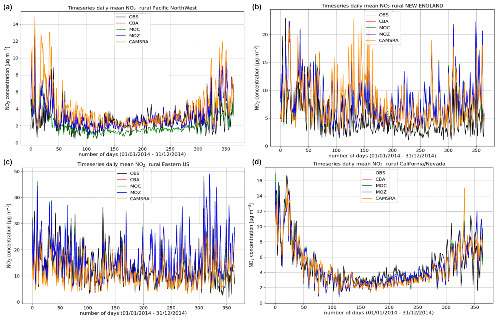
Table 9 Annual mean biases (µg m⁻³) and Pearson's R values for the comparison of surface NO₂ versus AirNow data for 2014.

In Fig. 13 we show comparisons of the daily mean variability in surface NO₂ in the simulations against daily mean composites assembled from the AirNow network for selected regions using rural stations only as defined in Table 6. The corresponding AMB and Pearson's R coefficients for all domains are provided in Table 9. The number of stations used for assembling the observational composite is lower (higher) than that used for surface O₃ (CO) and typically not measured at the same location (see Fig. 1 and Table 5). The uncertainty in the observations is higher than for the other longer-lived species and dependent on the instrumentation used in the local networks, especially for the lower concentrations. Except for the eastern US, New England and Colorado data (not shown), there is a notable annual cycle, with minima occurring during boreal summertime which is captured across the simulations. Mean daily biases for the various chemical modules are specific to each region, showing the influence of the chemical mechanisms across different chemical regimes. The AMB varies significantly across regions, with biases towards the west of the US being lower than the east of the US following the distribution of NO_x emissions. The highest correlation exists for California and Nevada (R = 0.84–0.86), and the lowest correlation is found for the eastern US (0.42–0.46).

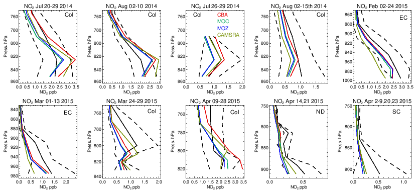
Figure 14 The same as for Fig. 6, but for tropospheric NO₂. Campaigns shown (top left to bottom right) are DISCOVER-AQ, FRAPPE, WINTER and SONGNEX.

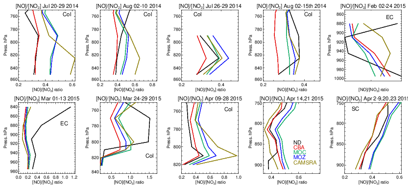
Figure 15 Comparisons of the $\left[\mathrm{NO}\right]/\left[{\mathrm{NO}}_{\mathrm{2}}\right]$ ratio for the lower troposphere from the various aircraft campaigns, with observational values shown in black. Campaigns shown (top left to bottom right) are DISCOVER-AQ, FRAPPE, WINTER and SONGNEX.

As for other species, tropospheric NO₂ profiles are compared against the corresponding aircraft composites for the various campaigns in Fig. 14, with the quantification of the biases given in Table S5. The corresponding profiles for tropospheric NO are shown in Fig. S2 and Table S7 in the Supplement. As for the other trace gases, the shape is captured relatively well, with the profile exhibiting a negative gradient with respect to pressure. Comparing the observational mean values in Table S4 shows that both Colorado and the eastern US have similar environments for NO_x levels (around 1.0–2.5 ppb). Model biases increase from summertime to wintertime under such NO_x-rich conditions. For IFS(CBA) there is no significant change in the biases for many months when compared to CAMSRA. In the various aircraft composites for Colorado, the mini-ensemble shows a significant peak around ∼ 820–830 hPa that is typically not seen in the observations and can result in positive bias in the LT. For NO, the corresponding biases are lower than for NO₂ with only marginal differences between chemical modules as shown in the Supplement. This suggests that differences shown in Fig. S2 are driven by nighttime chemistry that is outside the observational sampling window for most aircraft campaigns. For springtime, in Colorado and the south central US region there are significant positive biases for both NO and NO₂, especially for IFS(CBA), with overestimates of ∼ 50 %.

The $\left[\mathrm{NO}\right]/\left[{\mathrm{NO}}_{\mathrm{2}}\right]$ ratio (S) is an indication of the equilibrium position of the NO_x chemical system, as determined by the balance between fast titration of O₃ by NO plus conversion by peroxy radicals and its photochemical production from NO₂ photolysis. Low values for S are indicative of an equilibrium that favors O₃ production, and high values correspond to an equilibrium which favors O₃ destruction. A comparison of S between the different chemistry modules and those derived from in situ aircraft observations for the chosen campaigns are shown in Fig. 15. For summertime over Colorado the variability in S across the various campaigns ranges from 0.3 to 0.6, with significant differences across chemical modules. The profile shapes of S in the LT are captured well, but they show a lower variability in the chemical modules than in the observations. IFS(CBA) captures the correct S value in the LT for many of the months, while both other chemistry modules have a higher S, which moderates the O₃ biases shown in Table S1. In addition, CAMSRA has higher S values, typically overestimating resident NO mixing ratios (see Table S5), despite the application of data assimilation for NO₂. For the wintertime near the US East Coast, S is influenced by both daytime (high S) and nighttime (low S) measurements for February and mostly nighttime measurements for March, resulting in diverse behavior between the 2 months shown. Model biases of ∼ 0.1–0.2 occur across chemistry modules near the boundary layer. Interestingly, there is a significant increase in S in the measurements once the free troposphere (> 1.0) has been reached, which is not captured by any of the chemical modules, associated with an underestimation of NO in the model.

For springtime over Colorado there is marked difference in profile shape compared to the summertime, with much more vertical variability showing differences in transport and mixing patterns for this season not captured by the simulations. For other regions performance is better, with a very good agreement for the south central US region showing that for the correct conditions (chemical regime and transport) the chemical modules can capture a realistic description of the chemical system.

4.4 Tropospheric NO_y

The formation of O₃ is determined by the resident NO_x mixing ratios and the chain length in the chemical recycling between NO and NO₂ before termination to HNO₃ occurs. One rapid loss route for HNO₃ production is the conversion of nitrogen pentoxide (N₂O₅) on wet surfaces and aerosols, which has been directly observed during the WINTER campaign (Kenagy et al., 2018). For this campaign, N₂O₅ hydrolysis was shown to account for 58 % of the chemical loss of NO_x (Jaegle et al., 2018), with reaction of NO₂ with OH accounting for another third (thus the two most dominant chemical processes). In situ observations of N₂O₅ are rare, where daytime mixing ratios are typically of the order of tens of parts per trillion due to the efficient loss by photolysis and are therefore subject to high measurement uncertainty. During nighttime, surface observations range from 50 to 3000 ppt, with high daily variability (e.g., Wood et al., 2005; Brown et al., 2009). The WINTER campaign includes observations taken during night, where accumulations of N₂O₅ occur, allowing model evaluations to be made.

Evaluations against the nighttime N₂O₅ measurements from the WINTER campaign are shown in Fig. 16, along with the corresponding profiles of HNO₃. Unfortunately, no model data were available for N₂O₅ in the CAMSRA dataset for comparison. The formation of N₂O₅ involves the NO₃ radical, principally formed by the slow oxidation process from the reaction of NO₂ with O₃ during nighttime. Their relatively small biases for the WINTER campaign (see Figs. 6 and 14) provide some confidence in the flux of NO₃ production, where different reaction kinetics for thermal equilibrium are applied in each chemical module. Little difference exists across the chemistry modules for the simulated mixing ratios of N₂O₅, although a signature does exist for February regarding IFS(MOZ), which has 10 %–20 % higher mixing ratios in the LT. For IFS(MOZ), no N₂O₅ conversion on cloud particles and ice droplets is assumed (unlike the other chemistry modules).

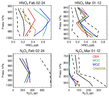
Figure 16 Comparisons of N₂O₅ and HNO₃ for the WINTER campaign using nighttime flights. The black line represents the observational mean value, with the associated standard deviation being shown as the dashed line.

For February a positive bias exists across chemical modules with respect to HNO₃ observations, where IFS(MOZ) counterintuitively has higher mixing ratios and biases (similar to IFS(MOC)) in spite of less efficient heterogeneous conversion. The corresponding N₂O₅ profiles indicate strong negative biases, thus suggesting too rapid hydrolysis into HNO₃. As described in Sect. 2.2, the conversion rate is computed in the IFS from the available surface area density (SAD) of clouds and aquated aerosols and the conversion frequency γ on these particles, (Brown et al., 2009), which is here assumed in the range of 0.01–0.02 depending on aerosol type; see Table 3. Derivations of γ(N₂O₅) from a chemical box modeling study based on the measurements across regions and scenarios taken during the WINTER campaign found a median value of 0.0143, with a spread of 2 orders of magnitude (∼ 0.001–0.1, McDuffie et al., 2018). This suggests that to reconcile the negative N₂O₅ model bias shown here the adopted γ(N₂O₅) needs to be made more variable. The inclusion of N₂O₅ conversion on clouds and ice particles for IFS(MOZ) would not improve on the biases shown here without modification of the efficiency of other N₂O₅ loss routes.

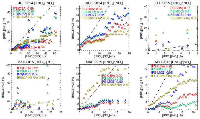
Figure 17 Comparisons of the observed $\left[{\mathrm{HNO}}_{\mathrm{3}}\right]/\left[{\mathrm{NO}}_{\mathit{\text{x}}}\right]$ ratio for selected months against the corresponding values from the ensemble members below 800 hPa. The values are binned with respect to the observations using a bin width of 0.75 with respect to $\left[{\mathrm{HNO}}_{\mathrm{3}}\right]/\left[{\mathrm{NO}}_{\mathit{\text{x}}}\right]$ and the correlation coefficients provided in each panel. Measurements are taken from FRAPPE, WINTER and SONGNEX campaigns to cover seasonality and location.

Comparing the $\left[{\mathrm{HNO}}_{\mathrm{3}}\right]/\left[{\mathrm{N}}_{\mathrm{2}}{\mathrm{O}}_{\mathrm{5}}\right]$ ratios to assess the efficiency of conversion while screening for very low and high values, Fig. S9 in the Supplement shows that the $\left[{\mathrm{HNO}}_{\mathrm{3}}\right]/\left[{\mathrm{N}}_{\mathrm{2}}{\mathrm{O}}_{\mathrm{5}}\right]$ derived from the chemical modules are only weakly correlated with those observed (R = 0.2–0.5), with the range of observational values being typically an order of magnitude lower than those seen in the mini-ensemble. For IFS(MOZ) during February there is a negative R value possibly linked to the lack of N₂O₅ conversion on clouds, with IFS(CBA) and IFS(MOC) having positive R values albeit with binned values which exceed 50 (too efficient conversion). For March, IFS(MOZ) has the highest correlation and lowest mean bias, which suggests conversion on aerosol surfaces dominates for this month and region. Table S4 shows that NO₂ has a small negative bias for these months, although no validation of the nitrate radical (NO₃) can be performed to determine whether the deficit in N₂O₅ is only due to heterogeneous processes. IFS(MOC) exhibits the most occurrences of high ratios for February (> 20), while for March both IFS(MOC) and IFS(CBA) have a similar incidence of high ratios (> 50).

The length of the NO_x cycle can be determined by examining the ratio between resident HNO₃ mixing ratios with the associated NO_x mixing ratios (denoted as R^′ = $\left[{\mathrm{HNO}}_{\mathrm{3}}\right]/\left[{\mathrm{NO}}_{\mathit{\text{x}}}\right]$), where high values are indicative of a large fraction of N that has been made inert (in the form of HNO₃). The resulting comparisons of R^′ calculated by accumulating values from selected days for each month (as for the vertical profile comparisons) for pressure levels below 800 hPa are shown in Fig. 17. A bin width of 0.75 in R^′ is used to calculate mean values in each respective bin. The resulting Pearson's R correlation coefficients are given in each panel.

For the spring and summer months over Colorado there is a high degree of correlation between measured and modeled R^′, with correlations in the range 0.8–0.9, except for August 2014, where the simulations become uncorrelated. For low R^′ values there is a tight agreement between the mini-ensemble members and the observational values. For higher R^′ values (> 10) the chemical modules exhibit low biases under high NO_x emissions, albeit with variable biases for HNO₃ (see Fig. S5 and Table S9 in the Supplement). Previous derivations of R^′ have found values in the range 0.8–10.4 for environments where NO_x is low (Huebert et al., 1990), which is in the range of those observed in the remote free troposphere. Biases for CAMSRA are overall much lower than those from the three recent chemistry modules during springtime.

Figure 18 The seasonal mean distribution of surface mixing ratios for gas phase HNO₃ across the US and Canada for JJA (top) and DJF (bottom) against seasonal composites of observations taken from the CASTNET network. The observational mean values and locations of the measurement stations are given as the diamonds located in each panel.

Both daytime and nighttime measurements are used for deriving the wintertime (February–March) correlations, where the observational range in R^′ is approximately half that derived for summertime. Correlations become much weaker, and the R^′ values are an order of magnitude higher for the mini-ensemble than those in the observations, indicating that the NO_x chain length for the chemistry versions is shorter than observed. One main difference is that uncertainties associated with heterogeneous conversion of N₂O₅ play a dominant role in HNO₃ production during nighttime, which may explain the reduced correlation. For CAMSRA, the high R^′ values (> 30) during February in the three chemistry modules do not occur.

To further evaluate the regional differences in HNO₃ across the chemical modules, we make seasonal comparisons of surface HNO₃ mixing ratios against observational composites taken from the CASTNET network throughout the US (Fig. 18). The maximal mixing ratios for HNO₃ occur near regions with high NO_x emissions. For JJA, differences between configurations are modest, with the largest percentual spread over the comparatively clean northern part. Comparing seasons shows that for IFS(CBA) during DJF much more HNO₃ exists towards the western US than for JJA. Instead, there is a significant reduction in IFS(CBA) during DJF on the US East Coast that is larger than for the other two modules.

Despite relatively small absolute values in OH mixing ratios during DJF, the significant percentual differences between modules (Fig. S1), could be responsible for differences in the direct production term across chemical modules, with overall higher HNO₃ mixing ratios in IFS(MOZ) and IFS(MOC) than IFS(CBA). In addition, there are uncertainties in HNO₃ loss through nitrate aerosol formation and deposition that contribute to uncertainties in HNO₃ burden, e.g., Nowak et al. (2010).

Spatial correlations r between the seasonal mean modeled and observed mixing ratios for the eastern and western US are approximately r = 0.5 for each of the chemistry modules for JJA. For this season the chemistry modules show an associated mean positive bias of between 0.3 and 0.4 ppb for the eastern US and almost no significant mean bias for the western US, which is due to some cancellation of positives and negatives for different locations.

The corresponding seasonal mean values for DJF show more divergence in correlation statistics, with r ranging from 0.07 to 0.24 for the eastern US and from 0.54 to 0.65 for the western US for the three chemistry modules. Associated mean biases are in the range 0.17–0.43 ppb (eastern US) and 0.41–0.51 ppb (western US), respectively. These evaluations indicate significant uncertainty regarding surface HNO₃ model capabilities, with overall positive biases. We refrain from further analysis of HNO₃, as this involves assessment of deposition and nitrate formation. Finally, it should be acknowledged that the CASTNET measurement network has been shown to have rather low mixing ratios when compared to alternative measurement networks (Lavery et al., 2009).

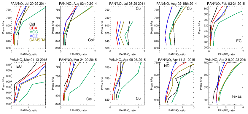
Figure 19 Comparisons of the ratio of $\left[\mathrm{PAN}\right]/\left[{\mathrm{NO}}_{\mathrm{2}}\right]$ derived from the corresponding mean values derived during each aircraft campaign. Campaigns shown (top left to bottom right) are DISCOVER-AQ, FRAPPE, WINTER and SONGNEX.

The significant differences in the seasonal distribution shown for NO₂ as diagnosed in Sect. 4.3 can be explained in part by variability in PAN production and loss across the various mini-ensemble members. A particularly large model spread was seen for DJF (Fig. S8 in the Supplement). Here, colder temperatures increase its tropospheric lifetime by suppressing thermal decomposition but simultaneously decrease its formation in the absence of biogenic and BB precursor emissions (Fischer et al., 2014).

Figure S7 in the Supplement compares resident mixing ratios of PAN against composites for the different aircraft campaigns, colocated with the measurements used for the evaluation of NO₂. It shows that for JJA, IFS(CBA) and CAMSRA typically underestimate PAN mixing ratios in the LT, where biases decrease as the temperatures get colder for the wintertime. For December–March, IFS(MOC) shows a positive biases of up to 100 %, indicating that PAN is too stable under cold conditions. This points at different reaction data employed compared to IFS(CBA) and IFS(MOZ) and a lower photolysis frequency. As a result, a significant overestimation in the fraction of NO_x exported out of the source regions will occur, as shown in the seasonal zonal mean PAN distributions in Fig. S8, where twice as much northerly transport occurs for IFS(MOC) compared to the other chemistry modules.

The ratio F, defined as F = $\left[\text{PAN}\right]/\left[{\mathrm{NO}}_{\mathrm{2}}\right]$, can be used to examine the ability of the chemical modules to capture the correct partitioning of resident NO_x into PAN, which can then be transported out the source regions by convective uplift and long-range transport affecting background O₃ budgets (Fischer et al., 2014). In general, the observations show an increase in F with respect to altitude, with F typically ranging between 0 and 1 during summertime and 0- and 2 during wintertime (Fig. 19). For most months and regions, IFS(CBA) and IFS(MOZ) provide accurate simulations of the vertical variability in F values between 850 hPa and the surface. IFS(MOC) generally has a positive bias in F, particularly during wintertime, where F is up to a factor of 2 higher than that observed. This is indicative of a too stable PAN in this chemistry version, which affects the O₃ production efficiency via the availability and distribution of NO₂.

During summertime over Colorado, IFS(MOC) exhibits good agreement in F in the lower atmosphere, with IFS(CBA) and IFS(MOZ) underestimating this by 0.03–0.05. Despite the updates to the NO_x chemistry in IFS(CBA), CAMSRA has slightly lower biases for summertime. For wintertime (springtime) towards the US East Coast (Colorado), F ratios for IFS(MOC) are nearly double those observed. However, agreement is quite good for North Dakota and South Dakota (ND) for April, showing the regional variability in the performance of the chemical modules. As PAN is transported out of the boundary layer, the contribution of the loss rate due to photolysis increases (albeit with a low frequency thus allowing long transport lifetimes). This highlights the importance of a correct parameterization of the photolysis frequency across the various chemistry modules. The reaction towards the colder temperatures in the FT markedly affects lifetime, where different reaction kinetics are applied across chemical modules.

5 Conclusions

In this study we have presented a detailed description of the recent updates that have been made to the chemistry modules that are integrated in the ECMWF IFS global model for the purpose of performing global air quality forecasts. We have evaluated a set of three simulations covering the years 2014 and 2015, using the latest model configuration as developed in an experimental version of the ECMWF IFS cycle 47R1. This provides insight in the performance of the modeling of trace gases (here excluding data assimilation) in the CAMS global system. This study has focused on lower tropospheric composition for the contiguous United States with an emphasis on tropospheric O₃, NO₂ and CO. We also included comparisons against the most recent reanalysis dataset that is based on a previous CAMS configuration (CAMSRA). This provides a reference to assess the performance of the current model configurations compared to this established dataset.

By comparing seasonal means in the lower troposphere between the various chemistry modules we have shown a strong seasonality in the regional inter-model differences for O₃, CO and NO₂ in the US. For O₃ these differences are limited to ± 5 % during boreal summertime, during which higher mixing ratios occur. The ability to capture the regional seasonality in surface concentrations for the background is somewhat region dependent, with relatively good agreement for the Pacific Northwest and an overestimation towards the US East Coast. Comparing seasonal composites against ozonesondes shows that there is generally good agreement in more remote locations and high positive biases of 10–30 ppb for more polluted regions, especially at the surface near the US East Coast. Comparisons for more southern regions show lower mean daily biases in the south central US and California and Nevada regions, with limited correlation in the daily variability. For the Colorado region, there are biases of ± 6 ppb across chemistry modules (± 10 %–15 %). At the surface there are small negative biases of around 5 µg m⁻³ for IFS(CB05BASCOE) and 15 µg m⁻³ for CAMSRA. For boreal wintertime a significant variability in the O₃ production efficiency occurs across chemistry modules, resulting in IFS(MOCAGE) and IFS(MOZART) exhibiting increases in mixing ratios of +6 %–15 % and +20 %–25 % across a wide region as compared to IFS(CB05BASCOE), especially in the northern US. A significant positive bias in surface concentrations occurs for 2014 in the northern US, indicating too efficient O₃ production, whereas CAMSRA exhibits a significant negative bias. Other regions show less difference across the simulations.

Associated differences occur for the OH radical for both seasons, which leads to significant differences in the tropospheric distribution of CO of between 8 % and 20 %, especially during wintertime. In general, the seasonal cycle at the surface is captured well when compared to both ESRL background observations and surface AirNow, with IFS(MOZART) exhibiting the largest negative biases in northern US regions. When compared against aircraft observations, positive biases in CO of 10–20 ppb occur for the Colorado region during boreal summertime for IFS(CB05BASCOE), with IFS(MOCAGE) agreeing relatively well and IFS(MOZART) giving an underestimation of a few parts per billion. These biases turn negative for wintertime and spring, reaching underestimates of up to 10–35 ppb across the simulations for different regions and months. This leads to deficits of 30–35 ppb in the lower troposphere for IFS(MOZART). Analyzing similar aircraft comparisons for CH₂O for both seasons shows negative biases of CH₂O between 5 % and 40 % depending on the region, which contributes to the negative CO biases. Biases of CO for all chemical modules are typically larger than the CAMSRA dataset, which is strongly constrained by assimilation of CO observations from satellite retrievals.

As was the case for O₃, NO_x also shows a seasonal variation in the simulated inter-model differences within the order of 5 %–10 % for NO₂ and up to 50 % for NO. Comparing profiles for both trace gases against aircraft measurements shows significant negative biases exist for both NO and NO₂ for the NO_x-rich environment of Colorado across all chemical modules, indicating regional emissions that are too low. The performance of the three chemistry versions is overall better than for CAMSRA, which can be understood by the fact that when assimilating NO₂ into the CAMS reanalysis only limited changes occur to the surface NO₂ mixing ratios. Comparisons against AirNow surface observations show that the regional annual cycles are captured well across the simulations with negative biases and that they show only a weakly correlated daily variability.

Examining $\left[\mathrm{NO}\right]/\left[{\mathrm{NO}}_{\mathrm{2}}\right]$ ratios shows that the equilibrium between NO and NO₂ is mostly captured well by IFS(CB05BASCOE) in the boundary layer, with the other chemical modules overestimating the fraction of NO (albeit with lower NO_x mixing ratios). A strong correlation exists in the $\left[{\mathrm{HNO}}_{\mathrm{3}}\right]/\left[{\mathrm{NO}}_{\mathit{\text{x}}}\right]$ ratio across days for boreal summertime between the modeled and measured fields (R > 0.9), albeit with a negative model bias of ∼ 50 %. This is indicative of a lower NO_y burden in the simulations due to cumulative differences in emissions, chemistry, aerosol formation and deposition processes. For CAMSRA, the $\left[{\mathrm{HNO}}_{\mathrm{3}}\right]/\left[{\mathrm{NO}}_{\mathit{\text{x}}}\right]$ ratio is better overall. For nighttime under cold conditions, the $\left[\mathrm{NO}\right]/\left[{\mathrm{NO}}_{\mathrm{2}}\right]$ ratio is typically underestimated, implying a lack of NO regeneration by slow redox reactions.

There is generally an overestimation in HNO₃, both at the surface and in the free troposphere, which may be due to too efficient N₂O₅ hydrolysis on wet surfaces under some conditions. Model analysis suggests that this conversion on cloud surfaces is not a dominating term with respect to associated N₂O₅ comparisons for the US East Coast during the wintertime period.

One dominating factor regarding the seasonal distributions of NO₂ is the fraction stored as PAN and transported out the source regions. For boreal summertime, IFS(MOZART) simulates 20 %–50 % less resident PAN than IFS(CB05BASCOE), which contributes to the more efficient O₃ formation in IFS(MOZART). When comparing against aircraft profiles around Colorado for July and August, there is generally an underestimation in resident PAN of 40 %–60 % across chemical modules, suggesting a lack of VOC precursors and subsequent acetyl-peroxy radicals, in line with previous studies (Huijnen et al., 2019). For boreal wintertime, when there is an extended tropospheric lifetime under cold temperatures, significant positive biases in regional PAN were diagnosed as compared against aircraft profiles for IFS(MOCAGE), pointing at differences in model assumptions regarding the stability of PAN, as determined by the rate data employed. This is also reflected by the $\left[\text{PAN}\right]/\left[{\mathrm{NO}}_{\mathrm{2}}\right]$ ratios, which show a strong overestimate in IFS(MOCAGE) and require future developments.

As presented in this paper, a significant divergence in key air quality products simulated by each of the chemistry modules exists depending on seasonal and regional conditions. These are due to fundamental differences associated with the oxidative capacity and the regional efficiency for the production of tropospheric O₃, which are in turn determined by the chemical mechanism, the parametrizations that are adopted and the rate data used. In future studies, attention should be made towards (i) improvement of variability in surface O₃, CO, and NO₂ with respect to air quality observations by a joint effort of improving the emissions and deposition handling and improved diagnostics; (ii) further homogenization of the physical conversion processes across modules with respect to radicals and N₂O₅; (iii) improvement of the VOC tropospheric burdens to provide sufficient peroxy radicals for better PAN formation; and (iv) further investigation into what determines PAN mixing ratios under cold and low-light conditions in terms of dissociation and stability. Evaluation of model performance for other important polluted world regions, such as Europe and East Asia, will be the focus of future studies.

While analysis of the three chemistry modules in CAMS provides a strong handle on uncertainties associated with chemistry modeling, the further improvement of operational products additionally requires coordinated development involving emissions handling, chemistry and aerosol modeling, all complemented with data assimilation efforts.