the Creative Commons Attribution 4.0 License.
the Creative Commons Attribution 4.0 License.
 | 16 Jun 2022
GNOM v1.0: an optimized steady-state model of the modern marine neodymium cycle
Sophia K. V. Hines
Hengdi Liang
Yingzhe Wu
Steven L. Goldstein
Seth G. John
Spatially distant sources of neodymium (Nd) to the ocean that carry different isotopic signatures (εNd) have been shown to trace out major water masses and have thus been extensively used to study large-scale features of the ocean circulation both past and current. While the global marine Nd cycle is qualitatively well understood, a complete quantitative determination of all its components and mechanisms, such as the magnitude of its sources and the paradoxical conservative behavior of εNd, remains elusive. To make sense of the increasing collection of observational Nd and εNd data, in this model description paper we present and describe the Global Neodymium Ocean Model (GNOM) v1.0, the first inverse model of the global marine biogeochemical cycle of Nd. The GNOM is embedded in a data-constrained steady-state circulation that affords spectacular computational efficiency, which we leverage to perform systematic objective optimization, allowing us to make preliminary estimates of biogeochemical parameters. Owing to its matrix representation, the GNOM model is additionally amenable to novel diagnostics that allow us to investigate open questions about the Nd cycle with unprecedented accuracy. This model is open-source and freely accessible, is written in Julia, and its code is easily understandable and modifiable for further community developments, refinements, and experiments.
- Article
(13615 KB) - Full-text XML
- BibTeX
- EndNote


Rare earth elements (REEs) have long been recognized to provide unique insight into ocean circulation and biogeochemical cycles (e.g., de Baar et al., 1983, 1985; Bertram and Elderfield, 1993; Elderfield, 1988; Elderfield and Greaves, 1982; German et al., 1995; Goldberg et al., 1963; Haley et al., 2014; Høgdahl et al., 1968; Lacan and Jeandel, 2001, 2004; Piepgras and Jacobsen, 1992; Piper, 1974; Sholkovitz and Schneider, 1991; Zheng et al., 2016). Isotopic variations in neodymium (Nd), in particular, have been extensively used as a tracer of ocean circulation, which plays a fundamental role in Earth's climate over a wide range of timescales, from millennia to millions of years (e.g., Adkins, 2013; van de Flierdt et al., 2016a; Frank, 2002; Goldstein and Hemming, 2003; Piepgras and Wasserburg, 1980; Sigman et al., 2010; Tachikawa et al., 2017).
Neodymium is part of a long-lived isotope system. Samarium-147 (147Sm) decays to neodymium-143 (143Nd) with a half-life of 106 Gyr. While the Sm:Nd ratio varies within the earth, these ratios are remarkably similar in most rocks in the continental crust and across the geological timescale and about 40 % lower than the bulk earth Sm:Nd (DePaolo and Wasserburg, 1976; McCulloch and Wasserburg, 1978; Goldstein et al., 1984), and as a result, the εNd values in continental rocks generally directly reflect the average crustal age. Therefore, the Nd isotope ratio is mainly a reflection of the amount of time the Nd in a rock has been a part of the continental crust, with lower values indicating older ages and longer crustal residence times (DePaolo and Wasserburg, 1976; McCulloch and Wasserburg, 1978; Goldstein and Hemming, 2003; Jeandel et al., 2007; van de Flierdt et al., 2016a; Robinson et al., 2021). Because R variations are typically small, Nd isotope signatures are usually defined as follows:
expressed in parts per 10 000 (![]() ; DePaolo and Wasserburg, 1976), where R is the measured ratio, and the chondritic uniform reservoir (CHUR) represents an estimate of the average Nd isotope ratio of chondritic meteorites and the bulk earth. For consistency with previously published data, we use RCHUR=0.512638 from Jacobsen and Wasserburg (1980), rather than the updated value from Bouvier et al. (2008).
; DePaolo and Wasserburg, 1976), where R is the measured ratio, and the chondritic uniform reservoir (CHUR) represents an estimate of the average Nd isotope ratio of chondritic meteorites and the bulk earth. For consistency with previously published data, we use RCHUR=0.512638 from Jacobsen and Wasserburg (1980), rather than the updated value from Bouvier et al. (2008).
Early measurements of εNd in seawater (Piepgras and Wasserburg, 1980) and ferromanganese oxide crusts (Elderfield et al., 1981; Goldstein and O'Nions, 1981; O'Nions et al., 1978; Piepgras et al., 1979) showed systematic variation across the ocean basins, with the lowest εNd values in the North Atlantic (−14 ![]() to −10
to −10 ![]() ),
the highest values in the Pacific (−5
),
the highest values in the Pacific (−5 ![]() to 0
to 0 ![]() ),
and intermediate values in the Southern Ocean (−11
),
and intermediate values in the Southern Ocean (−11 ![]() to −8
to −8 ![]() ).
The latter value broadly reflects mixing between waters from the North Atlantic, which are influenced by old continental terrains in northern Canada and Greenland, and the Pacific, which is influenced by mantle-derived volcanics (van de Flierdt et al., 2016a; Frank, 2002; Garcia-Solsona et al., 2014; Goldstein and Hemming, 2003; Goldstein and O'Nions, 1981; Lambelet et al., 2016; Piepgras and Wasserburg, 1980; Stichel et al., 2012a).
These observations led to the recognition that εNd values could be used to trace mixing between North Atlantic and Pacific waters over time, thus making εNd a potentially powerful paleoceanographic tracer.
).
The latter value broadly reflects mixing between waters from the North Atlantic, which are influenced by old continental terrains in northern Canada and Greenland, and the Pacific, which is influenced by mantle-derived volcanics (van de Flierdt et al., 2016a; Frank, 2002; Garcia-Solsona et al., 2014; Goldstein and Hemming, 2003; Goldstein and O'Nions, 1981; Lambelet et al., 2016; Piepgras and Wasserburg, 1980; Stichel et al., 2012a).
These observations led to the recognition that εNd values could be used to trace mixing between North Atlantic and Pacific waters over time, thus making εNd a potentially powerful paleoceanographic tracer.
More recently, the GEOTRACES program was created to better understand the sources and cycling of trace elements and isotopes in the ocean and how they impact broader marine biogeochemical cycles. The GEOTRACES Science Plan (GEOTRACES Planning Group, 2006) identified Nd isotopes as a key trace element or isotope that is expected to be measured on all GEOTRACES cruises because of its use as a paleoceanographic proxy. Thanks to this international effort, considerable amounts of new Nd concentration and isotope data have been generated in recent years, collected notably in the GEOTRACES Intermediate Data product 2017 (IDP17; Schlitzer et al., 2018), which increased the Nd data inventory by about 50 %, and post-IDP17 GEOTRACES data yet to be released in future data products.
To gain the most useful and accurate information from these observations, however, it is paramount to understand their modern ocean biogeochemical cycles and tracer budgets. Neodymium and other REEs enter the ocean via rivers, submarine groundwater discharge, eolian deposition, pore waters, and/or interaction with sediments (Fig. 1). Once in the ocean, they are redistributed by the ocean circulation, scavenged by particulate matter, and exit the ocean via sedimentation and incorporation into authigenic ferromanganese oxides (Frank, 2002; Byrne and Kim, 1990; Elderfield, 1988; Elderfield et al., 1981; Elderfield and Sholkovitz, 1987; Sholkovitz et al., 1989, 1994, 1992; Haley et al., 2004; Blaser et al., 2016; Du et al., 2016). While most sources of REEs to the ocean have likely been identified, there are still large uncertainties associated with the magnitudes of these different fluxes due to the inherent challenges of measuring sources that are temporally variable and globally widespread.
Models of the marine Nd cycle, in conjunction with seawater measurements, offer a way to constrain the magnitudes and isotopic compositions of these various inputs to the ocean and identify the most important sources. Of the distinct types of models, the following four have been used to simulate the modern ocean Nd cycle: simple box models, ocean general circulation models (OGCMs), steady-state circulation models, and boundary propagation models, each with their strengths and weaknesses (Table 1). Some of these models have explicitly tracked the concentrations of each Nd isotope (143Nd and 144Nd, thus allowing for the estimation of the Nd concentration and its isotopic composition), while other models have simply tracked εNd as a single conservative tracer.
Bertram and Elderfield (1993)Tachikawa et al. (2003)Du et al. (2020)Arsouze et al. (2007)Arsouze et al. (2009)Arsouze et al. (2010)Rempfer et al. (2011)Gu et al. (2019)Gu et al. (2020)Pöppelmeier et al. (2020)Jones et al. (2008)Siddall et al. (2008)Du et al. (2020)Table 1Previous modeling studies. Note: GCM is general circulation model, and TMI is total matrix intercomparison.
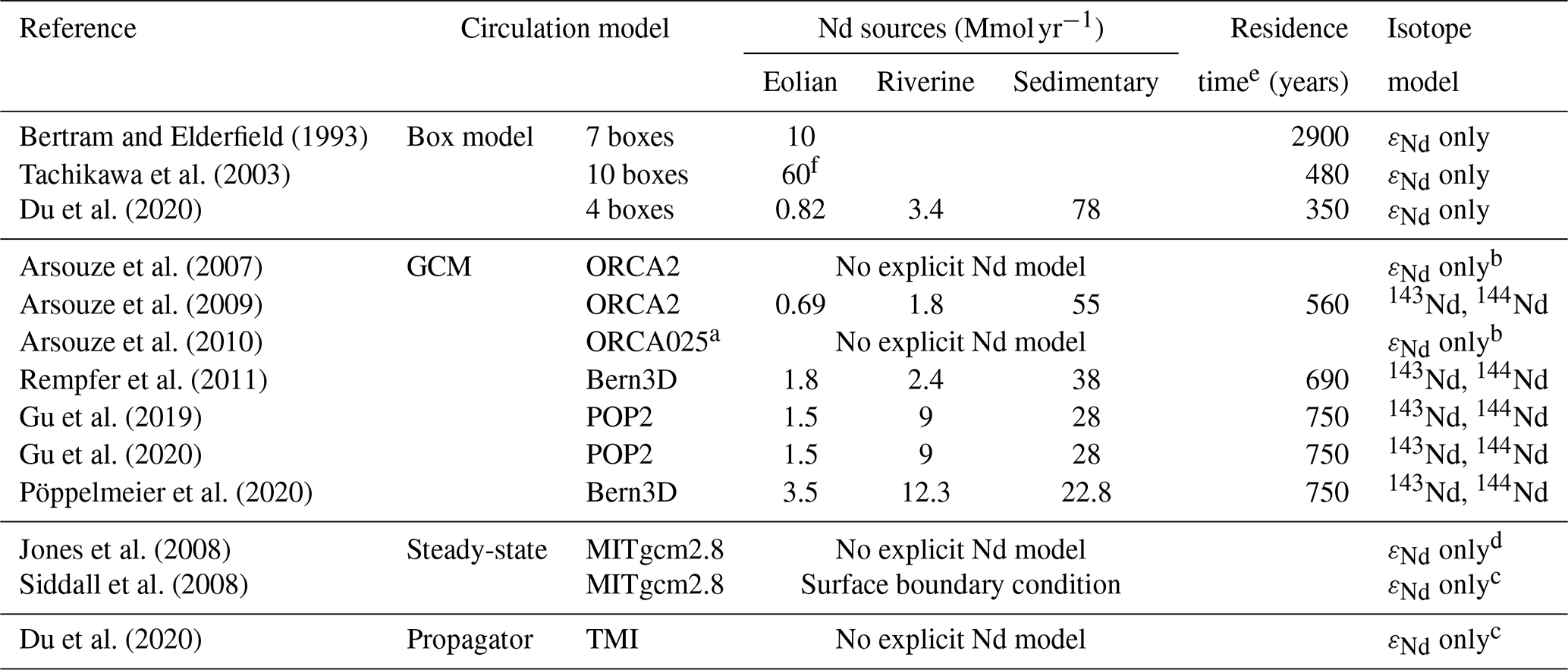
a Only the Pacific is modeled. b With deep boundary condition. c With surface boundary condition. d With deep and/or surface boundary conditions. e Bulk residence time estimated from the total Nd source magnitude for an ocean volume of 1.32×10¹⁸ m3 and a mean Nd concentration of 22 pM. f Total exterior surface flux calculated from their model, 90 % of which is missing compared to their estimate based on observations.
Box models typically refer to models consisting of 10 or fewer well-mixed boxes that exchange tracer with each other through prescribed mixing and overturning rates. Owing to their small size, box model simulations are the fastest to run and require very little computational power. Thus, they facilitate parameter optimization and scientific exploration by allowing for quick experimentation. For example, box models have been successfully used to determine that Nd must exchange between seawater and particles in the water column or at the sediment–water interface (Bertram and Elderfield, 1993) and that riverine and eolian sources are not sufficient to explain regional εNd variability (Tachikawa et al., 2003). However, very low spatial resolution prevents box models from capturing many important features of ocean circulation.
Ocean general circulation models sit on the other end of the spectrum of computational complexity, with better spatial resolution and resolved physics. Their computational costs generally prohibit systematic parameter space exploration or parameter optimization. These models have thus been used primarily to run well-defined experiments that target specific hypotheses, such as the importance of continental margin sources (boundary exchange) on εNd distributions, either as the sole source of Nd to the ocean (Arsouze et al., 2007, 2010) or an additional source to rivers and eolian deposition (Arsouze et al., 2009; Rempfer et al., 2011; Gu et al., 2019, 2020). To our knowledge, only Rempfer et al. (2011) and Gu et al. (2019) have attempted to optimize a Nd cycling model, using the low-resolution Bern3D OGCM and 3∘ resolution Community Earth System Model (CESM1.3), respectively, and each optimizing only two parameters.
More recently, a new class of steady-state models has emerged with unique potential to combine the advantages of OGCMs with the computational speed of box models. These models do not resolve the physics at runtime and, instead, rely on a prescribed, steady-state circulation. They can thus directly solve for the steady-state solution of the three-dimensional tracer equations, avoiding costly spin-ups, and drastically reducing simulation times. Thus far, to our knowledge, these models have only been used to test the top-down hypothesis by propagating a surface boundary condition into the ocean interior. Using the transport matrix method (TMM; Khatiwala et al., 2005; Khatiwala, 2007), Jones et al. (2008) showed that conservative mixing and advection from the surface alone cannot reproduce interior εNd observations, while Siddall et al. (2008) showed that including reversible scavenging captures the observed decoupling between quasi-conservative εNd and nutrient-like Nd concentration ([Nd]) distributions (the Nd paradox; Goldstein and Hemming, 2003).
The fourth class of models, which we have termed boundary propagation models, entirely bypasses expressing fluxes between model grid cells by connecting interior grid cells directly to the surface, using the total matrix intercomparison method (TMI; Gebbie and Huybers, 2010). Specifically, boundary propagation models estimate the fractional contribution of each surface grid cell to each interior grid cell. These models have been used to explicitly test the conservativeness of Nd isotopes as a tracer, since they do not incorporate external fluxes of Nd or internal cycling processes, and can thus only be used to simulate conservative transport. Indeed, similar to the experiment of Jones et al. (2008) referenced above, Du et al. (2020) used the TMI to inquire how well interior εNd values can be explained by conservative mixing and advection alone.
Our goal is to fill the current gap in the marine Nd modeling landscape and leverage the largely unexplored benefits of steady-state circulation models. Hence, here, we present the Global Neodymium Ocean Model (GNOM) v1.0, a mechanistic model of the modern ocean Nd cycle embedded in a state-of-the-art, steady-state estimate of the modern ocean circulation from the Ocean Circulation Inverse Model version 2 (OCIM v2.0; DeVries and Primeau, 2011; DeVries, 2014; DeVries and Holzer, 2019). The computational efficiency afforded by the model allows us to objectively optimize the model's parameters, making GNOM v1.0 the first inverse model of the Nd cycle and producing a good match to observations.
The GNOM v1.0 thus provides the community with a realistic yet computationally affordable tool to model the marine Nd cycle that we hope will be used to further improve our understanding of Nd cycling in the ocean. The model code and its optimization script are available publicly on GitHub at https://github.com/MTEL-USC/GNOM (last access: 26 May 2022). We used the free and open-source Julia language (Bezanson et al., 2017) and its packages, AIBECS.jl (https://github.com/JuliaOcean/AIBECS.jl, last access: 26 May 2022) in particular (Pasquier, 2020a; Pasquier et al., 2022b), as our main development platform. Owing to its open-source design, simplicity, and computational speed, the GNOM v1.0 is ideal for Nd cycle investigations. Except for the GEOTRACES dataset which must be downloaded manually, the GNOM is self-contained and version controlled, making it easy to reproduce simulations.
Additionally, the steady-state formulation of the GNOM is amenable to novel Green-function-based diagnostics that can provide important new insights into major open questions on the marine Nd cycle. Green functions (sometimes spelled Green's functions) can be used for solving ordinary differential equations with an initial condition and/or boundary values (see, e.g., Morse et al., 1953). In our case, they can be thought of as the [Nd] responses to unit local sources of Nd and allow us to partition [Nd] or εNd into components of interest, such as Nd from a particular source or location. Here, we introduce new partitions of Atlantic Nd and εNd (following, e.g., Holzer et al., 2016; Pasquier and Holzer, 2017, 2018; Holzer et al., 2021) that are helpful for disentangling the neodymium paradox (Siddall et al., 2008). We show that we can accurately partition [Nd] and εNd in the central Atlantic into contributions from northern- and southern-sourced waters. These preliminary diagnostics already reveal important information. They help quantify the conservativeness of εNd along water pathways and unveil underlying mechanisms by evaluating the effects of local sources and sinks. Detailed investigations of these diagnostics are out of the scope of this study and will be carried out in future work using a subsequent version of the GNOM with more finalized parameter values. We invite paleoceanographers and modelers alike to use the GNOM v1.0 model, to improve its implementation, to explore its capabilities, and thus to contribute to quantitatively answering long-lasting questions on the Nd cycle.
Neodymium concentrations are controlled by the interplay between circulation, external sources, and reversible scavenging and burial in the sediments (Fig. 1). These components completely define the state of the Nd cycle in our Global Neodymium Ocean Model (GNOM) v1.0. The three-dimensional partial differential equation for the Nd concentration tracer is discretized onto the grid of the Ocean Circulation Inverse Model (OCIM v2.0; DeVries and Holzer, 2019), yielding a system of 200 160 ordinary differential equations. Reorganizing the discretized three-dimensional arrays into column vectors, the steady-state tracer equation is recast in matrix form, as follows:
where is the modeled Nd concentration vector, Tcirc is the OCIM v2.0 advection–diffusion operator or transport matrix, Tscav is the reversible-scavenging matrix, and the sk are the external sources of neodymium. Note that and sk are 200 160-element column vectors and that Tcirc and Tcirc are sparse 200 160×200 160 matrices, such that the linear system represented by Eq. (2) can be solved in a few seconds on a modern laptop via lower–upper (LU) factorization and forward and backward substitution (often referred to as matrix inversion).
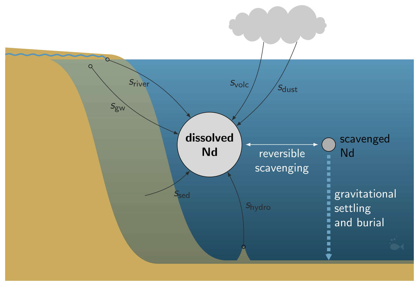
Figure 1Diagram of the Nd cycle model as implemented in GNOM v1.0. External sources of dissolved Nd are represented by black arrows. Localized sources, rivers, groundwater, and hydrothermal vents are indicated by a small circle at the origin of their respective arrows. A fraction of Nd is reversibly scavenged and pumped downwards. A fraction of scavenged Nd that reaches the sediments is buried in the sediments and removed from the system. Nd is also continuously transported by the ocean circulation model (not represented in the schematic).
The global εNd distribution is determined by both the distribution of 143Nd and 144Nd. Following, e.g., John et al. (2020), instead of explicitly simulating two additional tracers, we recover εNd values by simulating a single additional fictitious tracer for R[Nd], which we denote by RNd (and its column vector by ). This is equivalent to assuming that 144Nd:Nd is constant, such that and nominally track [144Nd] and [143Nd], respectively, multiplied by this constant 144Nd:Nd. We omit stable isotope fractionation during scavenging because its effect is negligible compared to the effect of radioactive decay from 147Sm. Thus, in Eq. (2), only the external sources sk differ in their isotopic composition. Thus, in practice, is computed by solving Eq. (2) with the sources replaced by Rksk (element-wise multiplication), where Rk is the vector of the isotopic ratio of Nd injected by source k. The modeled εNd values are then given by the vector (where all the operations are element-wise).
2.1 Ocean circulation
The term in Eq. (2) captures the flux divergence of [Nd] as it is carried along the mean ocean currents of the model and mixed by subgrid-scale eddies. The advection–diffusion operator Tcirc is represented as a 200 160×200 160 sparse matrix. (Most of the entries of Tcirc are zero because water can only travel directly between neighboring grid cells.) It comes from the output of the OCIM v2.0 (DeVries and Holzer, 2019), which provides a state-of-the-art data-assimilated steady-state ocean circulation (DeVries and Primeau, 2011; DeVries, 2014; DeVries and Holzer, 2019). Physically, Tcirc can be interpreted as the equivalent of , where u is the climatological mean water velocity field, and K is an eddy-diffusivity matrix of which the horizontal component is slanted along isopycnals. The spatial resolution of its grid is fixed at a nominal 2∘ × 2∘ in the horizontal and consists of 24 vertical levels of increasing height with depth. We emphasize that the OCIM v2.0 is particularly suited to this type of model because it arguably provides the best available estimate of the current climate long-term large-scale ocean circulation, while it affords spectacular computational efficiency.
2.2 External sources
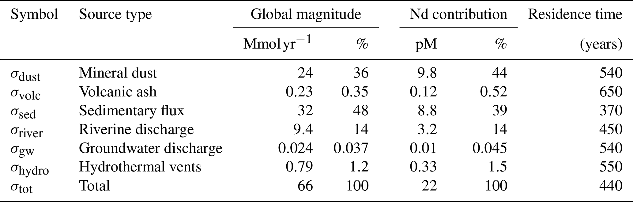
The GNOM v1.0 explicitly represents the following six sources of Nd into the ocean (Fig. 1): (i) atmospheric mineral dust deposition, sdust, (ii) atmospheric volcanic ash deposition, svolc, (iii) riverine discharge, sriver, (iv) groundwater discharge, sgw, (v) sedimentary remobilization (including pore water fluxes), ssed, and (vi) hydrothermal-vent release, shydro. The column vectors sk summed together constitute the total source of Nd (Eq. 2). Each source term is detailed in the following sections. Their spatial patterns and isotopic signatures are shown on Fig. 2, and their magnitudes and contributions to the total inventory of Nd are collected in Table 3.
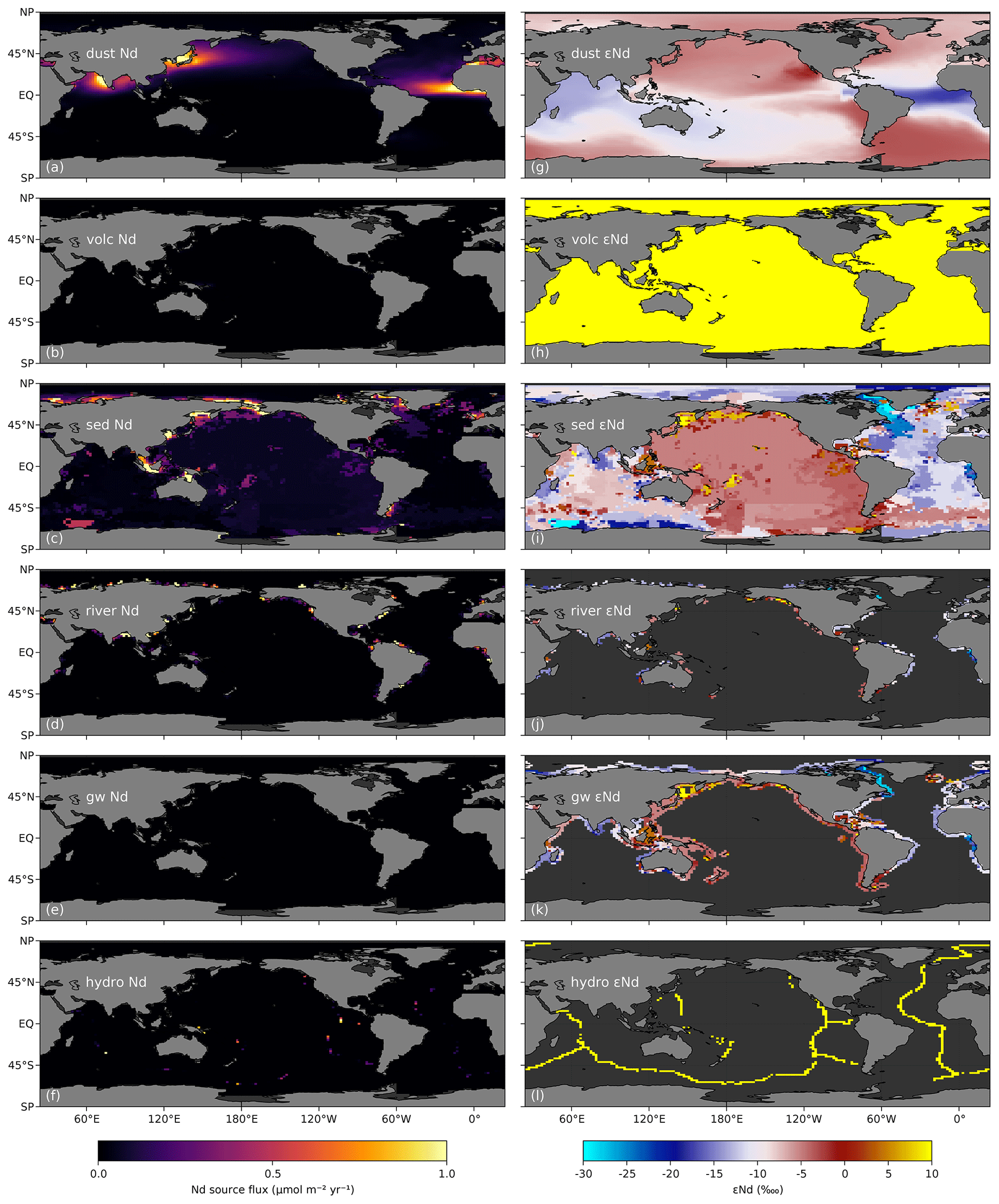
Figure 2Vertically integrated Nd sources and corresponding vertical mean εNd.
2.2.1 Eolian dust
We assume that atmospheric dust deposition injects Nd in the surface ocean only. That is, soluble Nd from dust is instantly released as dissolved Nd in the top layer of the model grid. Although it can vary with location and mineralogy (Goldstein et al., 1984), for simplicity, we assume a constant dust Nd content of µg g−1 (which is within the 11.93 to 45.76 ppm range of atmospheric dust observations of Goldstein et al., 1984). The spatial pattern of the dust source is prescribed by an atmospheric model output (Scanza et al., 2018) and is shown in Fig. 2a.
The isotopic signature of atmospheric mineral dust deposited on the ocean surface is not homogeneous (Goldstein et al., 1984). Instead, dust εNd varies with composition and mineralogy, which derives from its land origin. It is also likely that Nd solubility varies with composition and mineralogy. Thus, the GNOM v1.0 uses nine separate annual mineral dust deposition fields (dataset available from Adebiyi et al., 2020) from nine different regions. These dust deposition fields were generated by Kok et al. (2021a) and Kok et al. (2021b), who partitioned dust emissions according to nine different regions of origin, using the global climate model of Scanza et al. (2018). The nine regions we use are northwestern Africa (NWAf), northeastern Africa (NEAf), southern Sahara and Sahel (Sahel), Middle East and Central Asia (MECA), East Asia (EAsia), North America (NAm), Australia (Aus), South America (SAm), and southern Africa (SAf). Figure 3 shows the extent of these regions.

Figure 3Extent of the dust regions of origin (Kok et al., 2021a, b; Adebiyi et al., 2020) and their εNd values as optimized in GNOM v1.0. See the text for region names.
We assign a distinct Nd solubility and isotopic signature to each region of origin, controlled by the 2×9 corresponding parameters (denoted βr and εr for each region r; see the parameters in Table 2). The dust source of Nd into the ocean is hence given by the following:
where ϕdust,r is the dust deposition flux from region r taken from the Adebiyi et al. (2020) dataset and rearranged into a 200 160-element vector, Δz1 and z1 are the height and depth of the top layer of the model grid, z is the 200 160-element vector of depths, and MNd=144.24 g mol−1 is the molar mass of Nd. (All the operations in Eq. 3 are element-wise, and (z=z1) acts like a mask so that sdust only injects Nd in the top layer of the model grid.)
Each isotopic signature parameter εr uniquely defines the isotopic ratio of each region via , which is then used to compute the dust source for the RNd tracer via the following:
This allows for the eolian dust source to carry an elaborate and more realistic isotopic signature than previous models (Fig. 2g). Figure 3 also shows the optimized εr values of each region.
2.2.2 Volcanic ash
Despite a smaller atmospheric loading than mineral dust, we include volcanic ash as a separate, potentially important, eolian source of Nd because of its typically high reactivity and solubility compared to mineral dust. This reactivity partly reflects the high surface area of volcanic ash and the thermodynamic instability of volcanic glass (Gaillardet et al., 1999; Dessert et al., 2003). We use the geographic pattern of volcanic ash deposition, as used in the work of Chien et al. (2016) and Brahney et al. (2015), which provides estimates of the global deposition fields of dust and soluble iron from different aerosol types (mineral dust, volcanic ash, combustion fire, and so on). Assuming a constant neodymium content identical to dust, the volcanic ash source of Nd into the ocean is thus given by the following:
where ϕvolc is the column vector of the volcanic ash deposition flux from the Chien et al. (2016) dataset, and βvolc is the Nd solubility in volcanic ash. Similar to the dust source formulation, the magnitude of the volcanic ash source of RNd is controlled by the parameter εvolc, as follows:
where . (Note that Rvolc=Rvolc everywhere because the volcanic ash source comprises a single term, unlike the region-of-origin partitioned dust source.) The geographical patterns of the volcanic ash source and its uniform isotopic signature are shown in Fig. 2b and h.
2.2.3 Sediments
Sedimentary Nd is likely released via pore waters located in the upper few centimeters below the seafloor (e.g., Elderfield and Sholkovitz, 1987; Sholkovitz et al., 1989; Haley et al., 2004; Lacan and Jeandel, 2005; Wilson et al., 2013; Haley et al., 2017; Abbott et al., 2015a, b; Du et al., 2016, and references therein). The flux magnitude of this sedimentary release likely depends on sediment composition and reactivity (Lacan and Jeandel, 2005; Pearce et al., 2013; Wilson et al., 2013; Blaser et al., 2016, 2020). Other sedimentary environmental factors also likely play a role, such as oxygenation and organic matter flux (Elderfield and Sholkovitz, 1987; Sholkovitz et al., 1989, 1992; Haley et al., 2004; Lacan and Jeandel, 2005; Wilson et al., 2013). At high latitudes, mechanical glacial erosion likely increases sedimentary Nd fluxes by exposing fresh material and increasing surface area by producing fine particulates (Anderson, 2005; von Blanckenburg and Nägler, 2001), while increased bottom water eddy-kinetic energy may also enhance Nd release (Lacan and Jeandel, 2005; Gardner et al., 2018; Pöppelmeier et al., 2019).
There is no established quantitative flux model for sedimentary Nd release that works on the global scale, especially given the limited spatial coverage of direct sedimentary flux measurements (which are almost entirely restricted to the coastal northwestern Pacific). Therefore, the GNOM v1.0 implements the sedimentary Nd flux into the ocean as a flexible and optimizable function of depth z and local sedimentary εNd. The base sedimentary Nd flux, ϕ(z), is modeled as an exponential function of depth, as follows:
where ϕ0, ϕ∞, and z0 are optimizable parameters. The rationale behind the parameterization of Eq. (7) is versatility. For ϕ∞<ϕ0 and small z0, the flux profile is larger near the surface and smaller in the deepest parts of the ocean, while for ϕ∞>ϕ0 and large z0, the sedimentary flux increases quasi-linearly with depth (as in, e.g., Du et al., 2020, Fig. 1c). The optimization only enforces weak direct constraints on these parameters, allowing for any such profile shape. The optimized base Nd flux profile as a function of depth is shown in Fig. 4c.
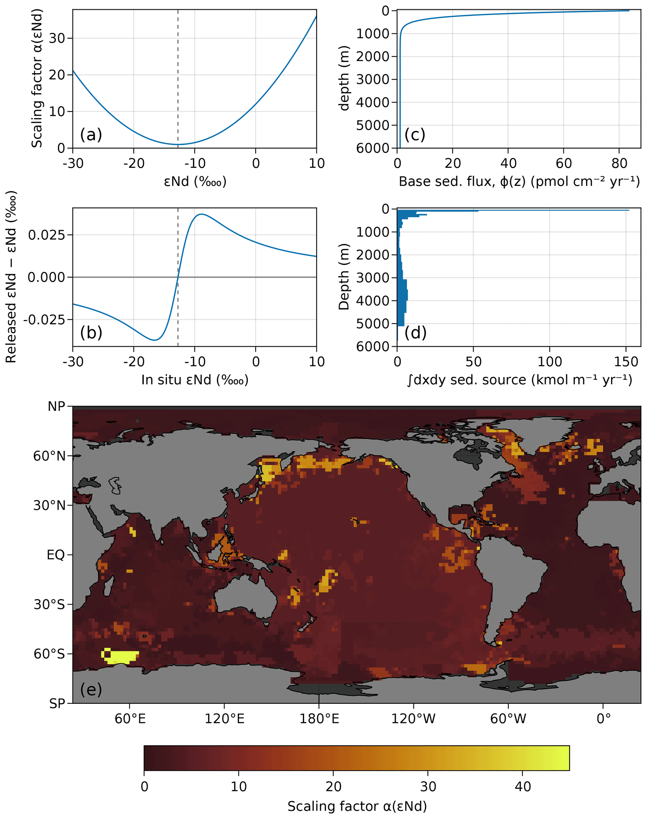
Figure 4(a) Sedimentary source enhancement as a quadratic function of observed εNd. (b) Difference between effectively released εNd and in situ εNd as a function of in situ εNd. (c) Sedimentary source flux profile as a function of depth. (d) Horizontally integrated sedimentary source. (e) Map of sedimentary reactivity/scaling factor α(εsed).
The base sedimentary flux is further scaled by a reactivity factor, α, which controls the effective sedimentary Nd release. Sediment reactivity is modeled via a simple parameterized quadratic function of local sedimentary εNd, as follows:
where the optimizable parameters a and c control the curvature and minimum of the quadratic, respectively, while ε10=10 ![]() is a normalization constant. (The specific value of ε10 is unimportant because it is absorbed by the optimizable parameter a during the optimization). Sedimentary εNd is taken from a modified version of the interpolated global map of sedimentary εNd of Robinson et al. (2021).
(Our modification caps the central and northern Pacific εNd values to a minimum of −5
is a normalization constant. (The specific value of ε10 is unimportant because it is absorbed by the optimizable parameter a during the optimization). Sedimentary εNd is taken from a modified version of the interpolated global map of sedimentary εNd of Robinson et al. (2021).
(Our modification caps the central and northern Pacific εNd values to a minimum of −5 ![]() because it appears that Robinson et al. (2021) artificially disconnected seafloor areas at the 180∘ meridian, resulting in εNd values that we flagged as too negative.) This quadratic parameterization is motivated by the fact that extreme sedimentary εNd values are often associated with rather fresh, and thus reactive, detrital material. We emphasize that this enhancement can be turned on or off, depending on the choice of parameters (a=0 turns it off). However, maybe coincidentally, extremely high εNd values are generally associated with relatively young volcanic Nd that is more reactive and readily soluble (Lacan and Jeandel, 2005; Pearce et al., 2013; Wilson et al., 2013; Blaser et al., 2016, 2020), and previous model studies have resorted to different enhanced Nd release parameterizations to achieve a similar effect (see, e.g., Pöppelmeier et al., 2020). The same is not necessarily true for rocks with extremely low εNd values; however, it so happens that much of the region around the Labrador Sea (Greenland and northern Canada) is currently, or was previously, glaciated, which has resulted in a large amount of fine-grained crystalline (and thus labile) detritus with extremely negative εNd (von Blanckenburg and Nägler, 2001).
The quadratic function α(εNd) is shown in Fig. 4a, and the resulting scaling factor for the global map is show in Fig. 4e.
because it appears that Robinson et al. (2021) artificially disconnected seafloor areas at the 180∘ meridian, resulting in εNd values that we flagged as too negative.) This quadratic parameterization is motivated by the fact that extreme sedimentary εNd values are often associated with rather fresh, and thus reactive, detrital material. We emphasize that this enhancement can be turned on or off, depending on the choice of parameters (a=0 turns it off). However, maybe coincidentally, extremely high εNd values are generally associated with relatively young volcanic Nd that is more reactive and readily soluble (Lacan and Jeandel, 2005; Pearce et al., 2013; Wilson et al., 2013; Blaser et al., 2016, 2020), and previous model studies have resorted to different enhanced Nd release parameterizations to achieve a similar effect (see, e.g., Pöppelmeier et al., 2020). The same is not necessarily true for rocks with extremely low εNd values; however, it so happens that much of the region around the Labrador Sea (Greenland and northern Canada) is currently, or was previously, glaciated, which has resulted in a large amount of fine-grained crystalline (and thus labile) detritus with extremely negative εNd (von Blanckenburg and Nägler, 2001).
The quadratic function α(εNd) is shown in Fig. 4a, and the resulting scaling factor for the global map is show in Fig. 4e.
Finally, to account for large glaciers that may produce fine-grained glacial flour from previously unexposed bedrock that likely contains reactive Nd (von Blanckenburg and Nägler, 2001), we additionally scale Nd release from the sedimentary source along the coast of Greenland by a factor αGRL. (For simplicity, we did not account for potentially enhanced Nd release in Antarctic because we assume that extreme εNd released by sediments in the Antarctic would be relatively rapidly mixed along the circumpolar current.) Combined with the reactivity α, the resulting sedimentary source is given by the following:
where αGRL is the vector equal to αGRL for grid cells against the coast of Greenland and equal to 1 otherwise, εsed is the column vector of the εNd map of Robinson et al. (2021) repeated at all depths throughout the water column, zbot is the vector of the depths of the bottom of each model grid cell, Δz is the vector of the height of each model grid cell, and ftopo is a mask equal to 1 for grid cells on the seafloor and equal to 0 otherwise. (Functions and operations in Eq. 9 are applied element-wise.) The horizontally integrated sedimentary source is shown Fig. 4d.
For the RNd sedimentary flux, we use the interpolated seafloor map of εNd values from Robinson et al. (2021) (modified with a −5 ![]() minimum in the Pacific north of 40∘ S). For grid cells with heterogeneous εNd in sediments, our quadratic implementation of the reactivity α as a function of εNd implies a statistical shift in the mean released εNd towards extreme values because extremely light or heavy Nd is released more efficiently.
Assuming that εsed represents the observed in situ mean of a normally distributed εNd sediment composition in each grid cell and a uniform global standard deviation σε within each grid cell, the εNd that is effectively released at any location, denoted , is given by the following:
minimum in the Pacific north of 40∘ S). For grid cells with heterogeneous εNd in sediments, our quadratic implementation of the reactivity α as a function of εNd implies a statistical shift in the mean released εNd towards extreme values because extremely light or heavy Nd is released more efficiently.
Assuming that εsed represents the observed in situ mean of a normally distributed εNd sediment composition in each grid cell and a uniform global standard deviation σε within each grid cell, the εNd that is effectively released at any location, denoted , is given by the following:
The difference between and in situ εsed is shown in Fig. 4b to shift εNd values by up to about ±0.03 ![]() .
In other words, for in situ εNd values lower than the minimum of α (dashed gray line in Fig. 4a and b), the released εNd value is pushed toward even lower values, and for in situ εNd values greater than the minimum of α, released εNd is pushed toward even larger values.
(The derivation of Eq. 10 is given in Appendix C). Applying
gives the sedimentary source of RNd as .
.
In other words, for in situ εNd values lower than the minimum of α (dashed gray line in Fig. 4a and b), the released εNd value is pushed toward even lower values, and for in situ εNd values greater than the minimum of α, released εNd is pushed toward even larger values.
(The derivation of Eq. 10 is given in Appendix C). Applying
gives the sedimentary source of RNd as .
2.2.4 Rivers
For riverine sources, we use the Global River Flow and Continental Discharge Dataset (Dai, 2017), originally described by Dai and Trenberth (2002) and later updated by Dai et al. (2009) and Dai (2016). This dataset provides an estimate of the volumetric flow rate of the 200 largest rivers on Earth. As a simplification, and to reduce the total number of free parameters in the model, we assume that all rivers share the same Nd concentration criver, which is the parameter that controls the global riverine source magnitude (see Table 2). (Future improvements of the GNOM could include optimizable [Nd] parameters for each individual major river, constrained by ranges based on observations.) Because the GNOM v1.0 does not resolve estuary removal processes, our criver is to be understood as an effective Nd concentration that implicitly accounts for Nd removal in estuaries and is thus the concentration that makes it into the ocean. Hence, the vector of the riverine source is given by the following:
where Qriver is the vector of the volumetric flow rates of the rivers from the dataset of Dai (2017) gridded (cumulatively) onto the OCIM v2.0 grid, and v is the vector of the volumes of the model grid cells. Note that in order to prevent numerical noise from the large gradients caused by the discrete nature of their distribution, we additionally artificially spatially smooth out the riverine sources by spreading it over neighboring grid boxes (see Fig. 2d).
Riverine εNd values are taken from the global map of interpolated sedimentary εNd by Robinson et al. (2021), which we also use for the sedimentary source, so that the RNd riverine source is given by . We note that the sedimentary εNd map of Robinson et al. (2021) overlays the nearest continental εNd signal where sediment thickness is more than 1 km, such that the εNd of the GNOM v1.0 riverine sources are mostly from continental measurements that lie within or close to the river drainage basins. Riverine εNd values are shown in Fig. 2j.
2.2.5 Groundwater
Neodymium also enters the oceans via coastal groundwater (Johannesson and Burdige, 2007). We use the coastal submarine and terrestrial groundwater discharge dataset of Luijendijk et al. (2019), described by Luijendijk et al. (2020), which provides the location and volumetric flow rate of 40 082 coastal watersheds. Similar to the riverine sources, we assume that [Nd] is constant across river watersheds and implicitly accounts for local Nd removal processes. The single parameter cgw is thus the effective groundwater concentration that makes it into the ocean and controls the global magnitude of the GNOM v1.0 groundwater Nd source (see Table 2). The groundwater Nd source is given by the following:
where Qgw is the groundwater volumetric flow rates from the dataset of Luijendijk et al. (2020), gridded cumulatively onto the GNOM grid. The pattern of sgw is shown in Fig. 2e.
Following Jeandel et al. (2007), we assume that the εNd of Nd released through groundwater is determined by the local lithogenic isotopic composition. However, instead of the dataset of Jeandel et al. (2007), we use the more recent Robinson et al. (2021) data, exactly like for the riverine source. These εNd values, which are located near the coast, are likely adequately representing the local lithogenic composition because Robinson et al. (2021) assign continental values where sediment thickness is greater than 1 km. The groundwater εNd values are shown on Fig. 2k.
2.2.6 Hydrothermal vents
A minor fraction of the marine neodymium budget presumably comes from hydrothermal vents, which deliver likely young Nd (high εNd) along the mid-ocean ridges (Piepgras and Wasserburg, 1985; Stichel et al., 2018). Here, we assume that the release of hydrothermal Nd is proportional to that of helium. For consistency, we use the mantle helium source field that was used in the data assimilation of the OCIM v2.0 (DeVries and Holzer, 2019). The global magnitude and εNd of the hydrothermal Nd source are set by parameters σhydro and εhydro, respectively (see Table 2), with the following:
where sHe is the vector of the 3He mantle source, and v𝖳sHe is its global magnitude, i.e., its volume integral, used here for normalization. (One can easily check that v𝖳shydro=σhydro.) The hydrothermal source of RNd is simply given by . Figure 2f and l show the spatial distribution of the hydrothermal Nd source and its εNd, respectively.
Arguably, the hydrothermal system as a whole acts as a net sink of Nd in the ocean (Stichel et al., 2018). As described in Sect. 2.3, the GNOM v1.0 does not include a parameterization of scavenging due to hydrothermal particles. Future versions of the GNOM should attempt to include such a removal process in order to properly balance the hydrothermal source and allow the εNd signature to be modified along hydrothermal vents without increasing the [Nd] concentration at the same time.
2.3 Reversible scavenging
Neodymium is removed from the system through scavenging onto particles. We follow, e.g., Bacon and Anderson (1982), Siddall et al. (2008), and Arsouze et al. (2009) and assume that dissolved and scavenged Nd are exchanged via a first-order kinetic reaction, as follows:
where X is a given particle type. The rate of change of [Nd] in Reaction (R1) can be written as follows:
with the following equilibrium constant:
We further assume that each scavenging particle type X has a constant settling velocity wX that dominates the transport rates of the ocean circulation. For each particle type X, we construct its flux divergence operator, denoted TX, such that TX x is the discrete equivalent of ∇⋅(wX [X]) (where x is the particulate concentration vector, and wX is the downward three-dimensional settling velocity vector). We use TX to compute the rate at which reversible scavenging adds or removes Nd in each grid box.
However, we avoid the explicit simulation of scavenged neodymium, XNd, by having a fraction of the dissolved neodymium pool sink to the box below as if it were adsorbed onto a falling particle. To do this in practice, we take advantage of the direct relationship between free and scavenged Nd, Eq. (15), assuming that Reaction (R1) operates on shorter timescales than either vertical particulate transport or ocean transport. (This assumption is common in models that include scavenging and simpler than resolving the adsorption/desorption rates dynamically (e.g., van Hulten et al., 2018).) Since dissolved and scavenged Nd are in equilibrium, Eq. (15) uniquely determines [XNd]=KX [X] [Nd], given the modeled [Nd] and the prescribed particle concentration [X] (from the four particle fields included in the GNOM v1.0, described below). Consequently, the corresponding partial downward flux of dissolved Nd is given by wX [XNd], where wX is the settling velocity of particle X. We further assume that a fraction fX of the scavenged Nd that reaches the seafloor is removed from the system, providing a net sink for our model. (Note that this is the same implicit approach as in the AWESOME OCIM (John et al., 2020).)
We consider four different particle types for scavenging Nd. (i) Scavenging by dust particles is modeled using the dust deposition fields of Kok et al. (2021b), assuming a vertically constant concentration as dust particles settle with velocity wdust=1 km yr−1 through the water column. (ii) Scavenging by particulate organic carbon (POC) is modeled using the three-dimensional POC concentration field from the work of Weber et al. (2018) and following the AWESOME OCIM implementation of John et al. (2020), with a settling velocity wPOC=40 m d−1. (iii) Scavenging by biogenic silica (bSi), or opal, is modeled using a simple, nutrient-restoring offline model of Si cycling described in Appendix A. (iv) A particle-independent scavenging is included to prevent the accumulation of Nd where the concentration fields of dust, POC, and opal are unrealistically low.
This fourth scavenging mechanism effectively behaves like spontaneous precipitation, and, as such, will be referred to as precipitation throughout this study (subscript prec). Precipitation is implemented by using a spatially uniform fictitious particle concentration of 1 mol m−3 that settles with velocity wprec=0.7 km yr−1. We note that, while this additional particle-independent scavenging sink could compensate for additional types of particles not currently implemented in the model, it is likely that more scavenging particle types are required for an accurate representation of the Nd cycle. These include hydrothermal particles (which should result in hydrothermal systems being a net sink; Stichel et al., 2018) and iron–manganese oxides (which are potentially the most important scavenging particles; Lagarde et al., 2020; Schijf et al., 2015; Sholkovitz et al., 1994). Overall, the scavenging transport operator is thus defined by summing the flux divergence for all particle types and using Eq. (15), as follows:
where DX is a diagonal matrix with diagonal x, which is the vector of the concentrations of particle type X. Hence, for each scavenging particle type X, the corresponding scavenging rate and downward transport is controlled by the concentration [X], the equilibrium constant KX, the settling velocity wX, and the burial fraction fX. Figure 5 shows maps and profiles of net scavenging rates for each particle type.
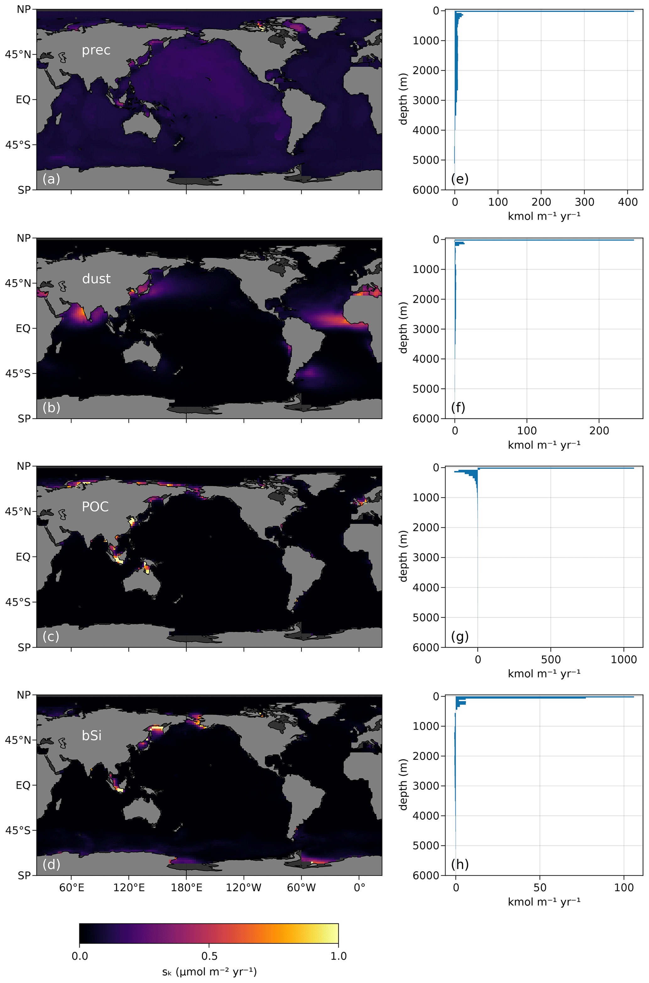
Figure 5(a–d) Vertically integrated and (e–f) horizontally integrated scavenging by precipitation, dust, POC, and opal particles, where positive values represent Nd removal and negative values represent a source of pumped Nd. Note that in panels (e)–(f), net scavenging rates in the top layer are positive and largest by construction because Nd can only be removed there, as opposed to all the layers below which can receive Nd from superjacent layers.
2.4 Optimization
The output of our model is governed by a set of 43 free parameters that control the magnitude and εNd of each source and the reversible scavenging and burial rates. The computational speed afforded by the model implementation allows us to jointly optimize almost all of these parameters by minimizing the mismatch of modeled and observed [Nd] and εNd values. This is done in practice by minimizing an objective function that quantifies the mismatch between model and observations, for a given set of parameters p.
2.4.1 Objective function
The mismatch with each observation is quantified by the square of the difference between the observed value and the modeled value from the closest grid cell. Because we use observations of [Nd] and εNd, the mismatch function, denoted f, depends on the 3D fields of the two modeled tracers ( and ). We also include an additional cost for parameter values themselves. The mismatch function is defined by the following:
where the first term represents the normalized mismatch between modeled and observed [Nd], the second term represents the normalized mismatch between modeled and observed εNd, and the last term represents the inverse of the likelihood of the model parameters. We detail each term below.
In Eq. (17), is a vector of all the [Nd] observations, and denotes the observed [Nd] at location r, which spans all the locations of observations, 𝒪Nd. (One can think of r as indexing the vector of observations .) We compare each observation with the model output from the closest model grid cell, denoted for simplicity. (Technically, the location of the observed and modeled value being compared may not match, in which case we use the closest wet model grid cell using a nearest-neighbor algorithm.) We use the same approach for εNd by comparing the modeled vector to the observed vector at the locations of each εNd observation. The ωNd and values, fixed at 1 in this study, control the relative contributions of the mismatches in Nd concentrations and εNd values. Given these, an error of 1 ![]() in εNd weighs the same as an error of about 4.5 pM.
in εNd weighs the same as an error of about 4.5 pM.
The third term of Eq. (17) adds a direct penalty constraint on the parameters to prevent them from reaching unrealistic values. If any parameter reaches a value close to the limits we impose in the model, then this third term will grow large; since the algorithm tries to minimize Eq. (17), it will push that parameter back to a more acceptable value. For each parameter pi, we prescribe a realistic domain Di and an initial guess (see Table 2) that we use to determine a reasonable prior probability distribution di and to randomize the initial parameter values. Specifically, each parameter with a semi-infinite range (from 0 to ∞) is given a lognormal prior of which the logarithm has mean equal to the logarithm of the initial guess and has variance equal to 1. Each parameter with a finite range is given a logit-normal prior that is scaled and shifted, such that its support matches the range Di exactly, such that the initial guess equals the median of di. For example, the ϕ0 parameter for the sedimentary flux at the surface is given the (0,∞) range and an initial guess of 20 . Taken as a random variable, the prior distribution of ϕ0 is the lognormal distribution, such that . (𝒩(μ,σ2) denotes the normal distribution with mean μ and variance σ2.)
For the performance and robustness of the optimization, we additionally perform a variable transform λi on each parameter using a bijection from the parameter domain Di to . This variable transform prevents parameters from reaching beyond their prescribed ranges. We also carefully chose the bijection, such that the prior distribution is normally distributed in the transformed parameter space and thus incurs an inverse log-likelihood that is quadratic, a property that benefits the performance of the optimization. In the case of the parameter ϕ0, which is transformed via the bijection , the corresponding transformed random variable is normally distributed by construction. For bounded parameters, such as βvolc, a shifted and scaled logit transform is applied, which also yields a transformed random variable that is normally distributed by construction.
The ωp value, fixed at 10−4 in this study, controls the relative size of the penalty for the parameters compared to the cost of Nd and εNd. It is chosen so that the [Nd] and εNd mismatch costs are generally about 2 to 3 orders of magnitude larger than the parameter penalty (although there is no bound on the parameter penalty for extreme parameter values). The primary role of this added parameter cost and the associated variable transform is to improve the convergence rate of the optimization and help prevent it from becoming stuck in valleys of parameter space (see, e.g., Nocedal and Wright, 1999).
The objective function depends on p only and is defined by the following:
where we have explicitly marked and as functions of the parameters p. That is, for any choice of parameters p, before evaluating the model mismatch as quantified by the objective function, we must first compute the vectors and by solving for the steady-state solution to Eq. (2). The gradient, , and Hessian, , of the objective function are computed using a combination of autodifferentiation and adjoint techniques available from within the AIBECS.jl package (Pasquier, 2020a; Pasquier et al., 2022b) or specifically developed in parallel for computational efficiency (F1Method.jl; Pasquier, 2020b).
2.4.2 Dissolved neodymium and εNd data
The [Nd] and εNd observations used in this study consist of the following three datasets: (i) the pre-GEOTRACES compilation of Nd and εNd data by van de Flierdt et al. (2016a), (ii) the GEOTRACES Intermediate Data Product 2017 (IDP17; Schlitzer et al., 2018) (including specifically Nd-linked publications; Stichel et al., 2012a, b, 2015; Garcia-Solsona et al., 2014; Basak et al., 2015; Fröllje et al., 2016; Lambelet et al., 2016, 2018; Behrens et al., 2018a, b), and (iii) our post-IDP17 compilation of data from the Indian Ocean (Amakawa et al., 2019), the Barents Sea (Laukert et al., 2018, 2019), the northern Iceland Basin (Morrison et al., 2019), the northwestern Pacific (Che and Zhang, 2018), the Kerguelen Plateau (Grenier et al., 2018), the southeastern Atlantic Ocean (GA08, Rahlf et al., 2020, 2019, 2021), the Bay of Biscay (Dausmann et al., 2020, 2019), the western North Atlantic (Stichel et al., 2020), the Arctic (Laukert et al., 2017a, d), and the Bermuda Atlantic Time-series Study (BATS; Laukert et al., 2017b, c). The spatial distribution of these observations as used in this study are shown in Fig. 6.
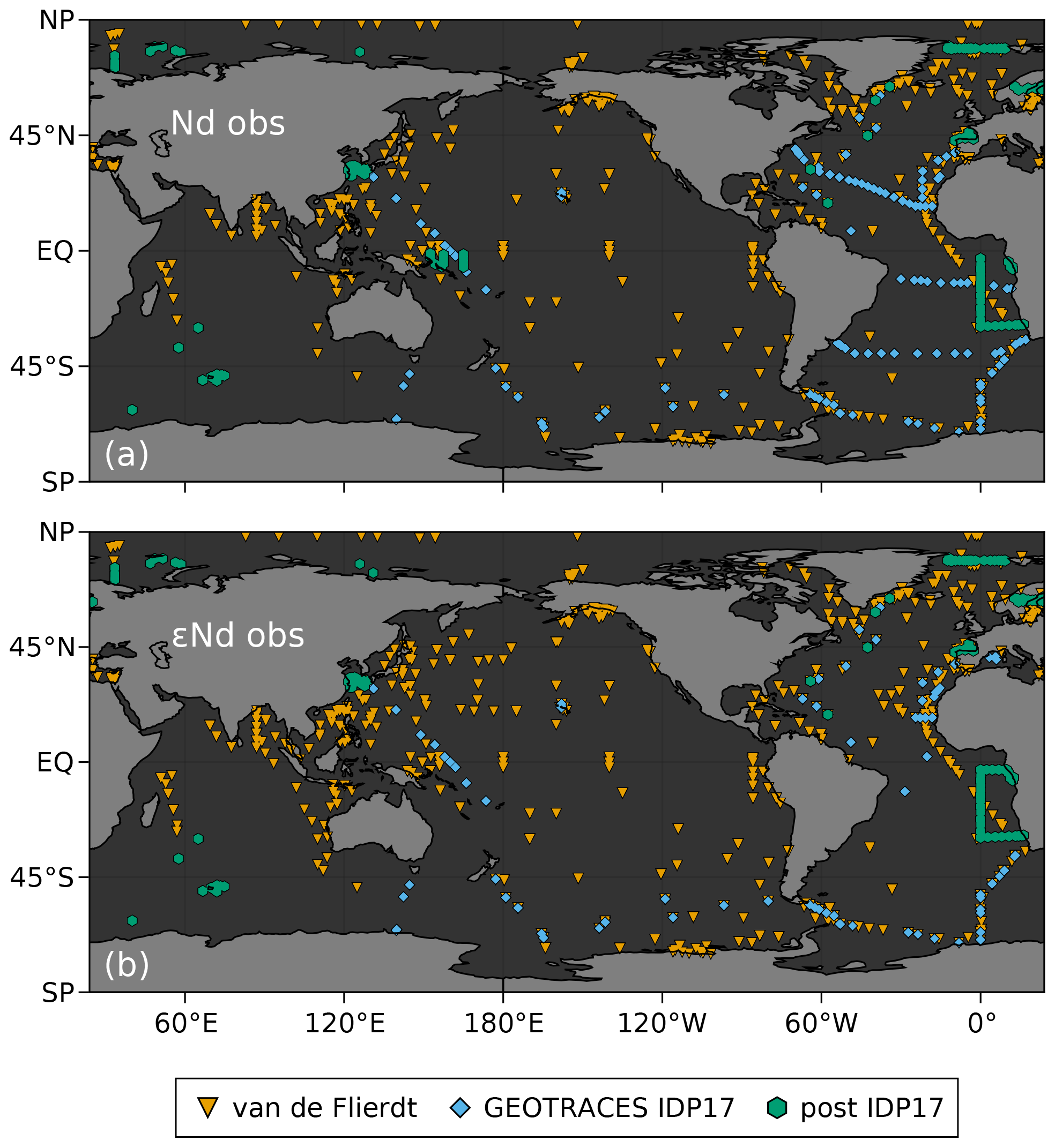
Figure 6Locations of (a) Nd and (b) εNd observations used in this study, labeled per the data source.
2.4.3 Minimization algorithm
We use the Newton trust region algorithm from the Optim.jl package (Mogensen and Riseth, 2018) to minimize the objective function . This requires, at every iteration, the objective function, its gradient, and its Hessian, which are evaluated using the F1Method.jl and AIBECS.jl packages (Pasquier, 2020a; Pasquier et al., 2022b; Pasquier, 2020b).
Thanks to the computationally efficient gradient optimization algorithm that leverages gradient and Hessian information, the entire optimization run takes a few hours on a modern laptop. In our experience, for comparison, using the more standard finite differences approach or an optimization algorithm that does not have access to derivatives would likely take multiple months.
Because the Newton trust region algorithm performs local rather than global optimization, we run multiple optimizations, starting from randomized initial parameter values sampled from the parameter distributions di (as shown in Fig. B1). Although not all optimization runs end up in the same state because of many local minima, we find that most of them converge towards similar solutions with a similar small objective function value, which we denote as our best estimate, and out of which all the figures in this work are created. Figure B1 also shows the initial values and final values of a dozen of optimization runs, with the best estimate shown in blue.
3.1 Parameter values
Our best estimate of the state of the Nd cycle is given by the set of parameters that minimizes the objective function defined in Eqs. (17)–(18). We emphasize that our estimate is determined by a local minimum of a specific parameterization, such that the best here is somewhat subjective. In all likelihood, there exist other models and other parameter choices which produce a similar fit to global observations, though we expect all such models to capture the same key features of global Nd biogeochemical cycling. Initial guesses and optimizable ranges for each parameter were determined from the literature and the expertise of authors. Initial guesses and final parameter values, along with unit, prescribed range, and a brief description, are given in Table 2. Parameter prior distributions, their randomized initial values, and final optimized values are shown in Fig. B1.
Table 2List of parameters. Realistic parameter ranges were prescribed based on the literature and the expertise of the authors. Final values have been rounded to three significant digits. Parameters without a range are not optimized (final value equals initial guess). Scavenging reaction constants, KX, are reported in units of inverse concentration of the particle X.
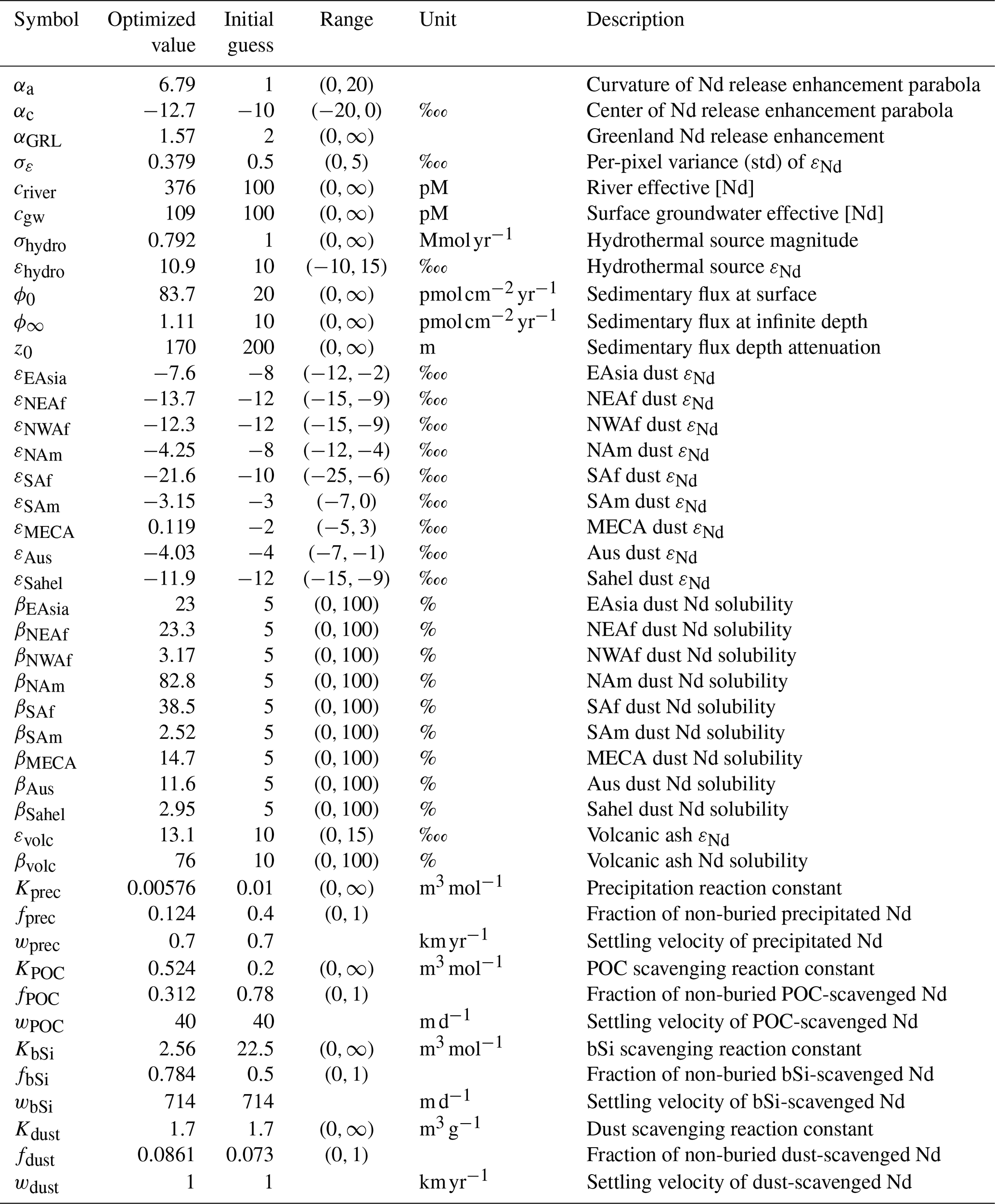
In Table 2, parameters without a range indicate that they were not optimized and held fixed at the given previous model or literature values. For example, in the case of scavenging by each particle type X, we only optimized KX and fX (not wX). As described in Sect. 2.3 above, the settling velocities for POC and bSi are not optimized and are instead fixed to match the values of their respective parent offline models. While there are no parent models for dust and precipitation, we do not optimize the corresponding settling velocities for these particle types either because KX and wX can perfectly compensate each other. For example, doubling KX while halving wX has no effect on Nd distributions and the objective function. Only their product, KX wX, which sets the strength of the scavenging pump through the operator matrix Tscav, appears in the tracer equations (see Eq. 16 or, e.g., John et al., 2020), such that these parameters cannot be easily optimized independently.
3.2 Fit to observations
The general fit to observations is illustrated in Fig. 7, which shows the percentiles of the cumulative joint probability distribution of the modeled and observed Nd concentrations and εNd values. Despite the slightly visible spread, most of the modeled–observed [Nd] and εNd values lie close to the 1:1 line, indicating a good match, with a root mean square error of about 6.80 pM and 2.09 ![]() , respectively.
, respectively.
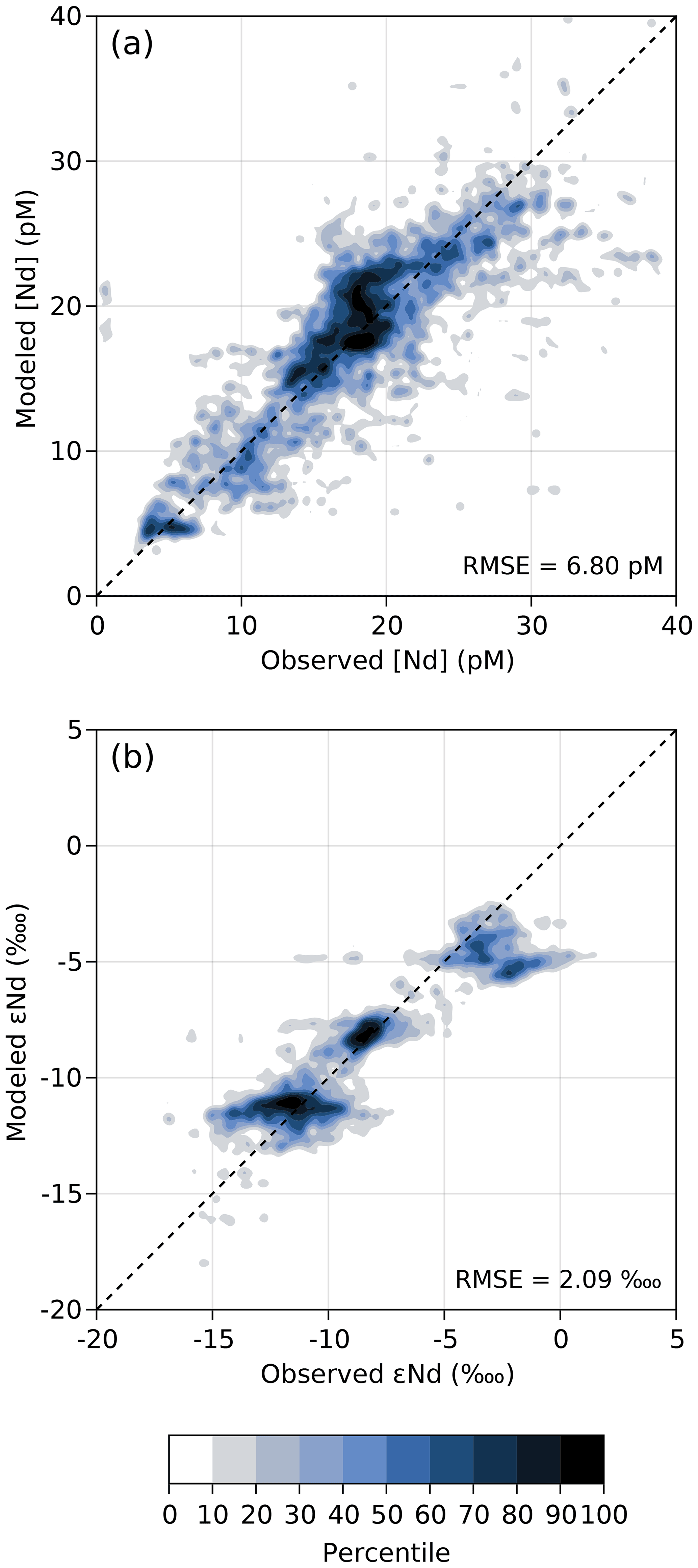
Figure 7Quantiles of the cumulative joint probability density functions of modeled and observed (a) Nd concentrations and (b) εNd values. Darker colors indicate a high density of data, such that n % of the modeled and observed data lie outside of the nth percentile contour. The closer the darker contours are to the 1:1 black dashed line, the better the fit.
While statistics such as Fig. 7 provide important information at a quick glance, they do not retain any geographical information, so that a more detailed investigation is required to fully assess the model's skill. Indeed, the deviations shown by [Nd] and εNd clusters slightly off the 1:1 line (Fig. 7) likely reflect groups of geographically proximate data points that may be symptomatic of systematic biases, which must be analyzed in further detail.
We explore the regional variations in the model's skill with depth in Fig. 8, which shows the basin-averaged profiles of modeled and observed [Nd] and εNd for the Atlantic, Pacific, Indian, and Southern oceans. Simulated [Nd] fits the nutrient-like profiles of basin mean observations and captures the bulk of interbasin variance fairly well despite systematic biases of about −3 pM in the mid-depth Atlantic,
+3 pM in the deep Atlantic, up to +6 pM in the mid-depth Indian Ocean, and −6 pM in the 4,250 m deep Southern Ocean (Fig. 8a–d). Similarly, for εNd values, we find an overestimate of about +1 ![]() below 700 m in the Atlantic and an underestimate of up to −2
below 700 m in the Atlantic and an underestimate of up to −2 ![]() in the Pacific, particularly near the surface, while the modeled and observed basin-averaged Southern Ocean profiles are a tight fit (Fig. 8e–h).
in the Pacific, particularly near the surface, while the modeled and observed basin-averaged Southern Ocean profiles are a tight fit (Fig. 8e–h).
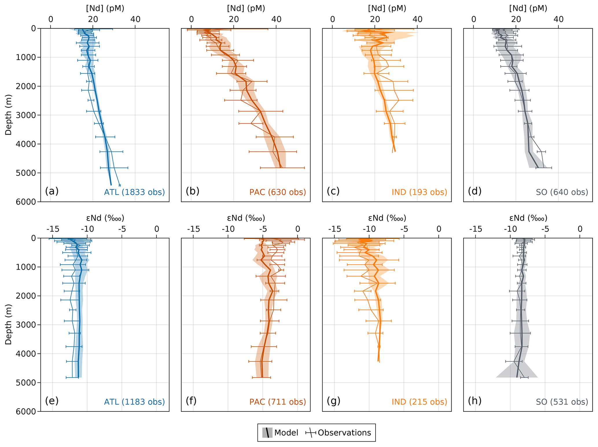
Figure 8Basin-averaged profiles of (a–d) Nd concentrations and (e–f) εNd values versus depth. The basins (Atlantic, Pacific, Indian, and Southern Ocean) with the number of observations for each tracer are reported in the bottom right corner of each panel. The mean and standard deviation of observations are calculated at each vertical grid level of the OCIM v2.0 grid and represented by the thin line and error bars. The mean and standard deviation of the model are represented by the thick line and lighter-colored ribbon.
We further assess the model skill by looking at GEOTRACES transects individually. Out of the 3483 observations of [Nd] that we use to constrain our model, 1575 (∼45 %) come from the IDP17 (Schlitzer et al., 2018) and were collected along the GA02, GA03, GA10, GA11, GAc01, GIPY04, GIPY05, GIPY06, GPc02, GPpr04, and GPpr05 cruises (Fig. 9b–l). Similarly, out of the 2988 εNd observations, 790 (∼26 %) come from IDP17 cruises GA02, GA03, GA11, GIPY04, GIPY05, GIPY06, GPc02, GPpr04, and GPpr05 (Fig. 10b–j).
Figure 9 reveals in detail how well GNOM output matches observational [Nd] data. The model captures the broad interbasin and intrabasin variations with high fidelity despite some slight mismatches. Specifically, Fig. 9c reveals overestimates of mid-depth and deep [Nd] in the west Pacific (cruise GPpr04) with an overestimated gradient with depth, potentially due to too large a sedimentary source or too strong scavenging. Mid-depth overestimates of [Nd] also appear in the Atlantic (GA03, GAc01, and GA10; Fig. 9h, j, k). However, the deepest [Nd] are underestimated in association with a generally underestimated vertical gradient, particularly along GA10. Hence, the [Nd] mismatches in the Pacific are suggestive of either too weak a deep sedimentary source or too efficient scavenging and burial in the deep. These systematically opposed mismatches between the Atlantic and Pacific are likely due to the optimization procedure, which balances out all the mismatches simultaneously. Future improvements in the GNOM that resolve these discrepancies could include different parameterizations of the sedimentary source and scavenging or the addition of a currently absent third mechanism, such as a nepheloid source or sink.
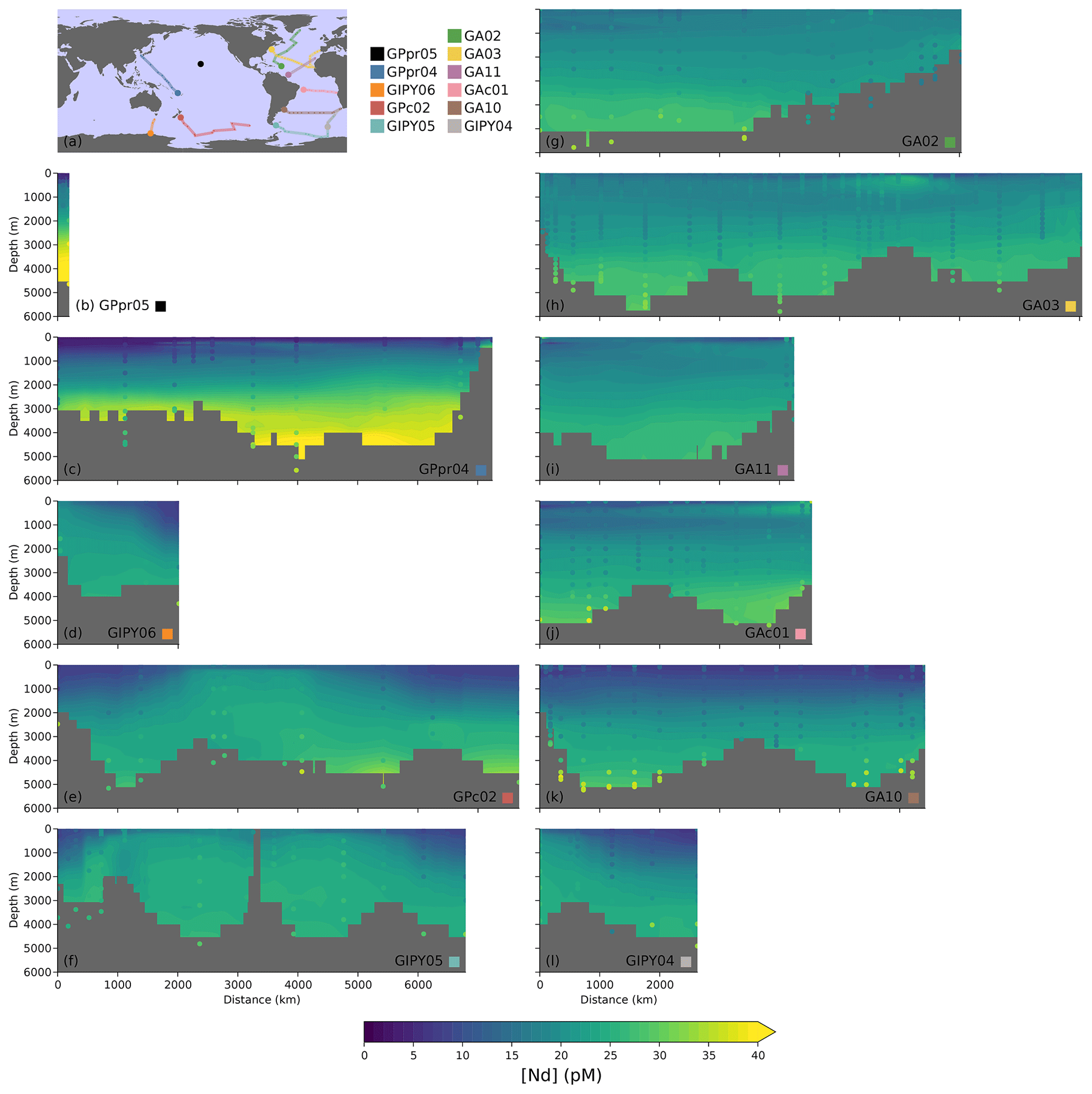
Figure 9(a) GEOTRACES cruise tracks with [Nd] observations. The legend layout matches the layout of the other subplots of the figure. (b–l) Modeled and observed [Nd] along GEOTRACES transects. Modeled values are shown as filled contours, while observed values are overlaid as a scatterplot.
Figure 10 shows modeled and observed εNd values along IDP17 cruise transects. While the observed interbasin variability is adequately represented, the GNOM does not perfectly capture the finer spatial details of observed εNd, suggesting that there is still room for model improvement. The model agrees well with observations along Southern Ocean transects (Fig. 10e, i, j; GPc02, GIPY04, and GIPY05). However, in the North Atlantic (e.g., Fig. 10f, GA02), the GNOM does not entirely capture a strong negative εNd plume along the North Atlantic Deep Water (NADW). Conversely, in the western Pacific (Fig. 10c; GPpr04), our model misses strongly positive surface εNd observations and instead displays a deep plume of positive εNd that is absent from the observational data. This is potentially due to missing mechanisms, sources, or sinks, the correct implementation of which would likely benefit from more observational εNd data in the Pacific and Indian basins.
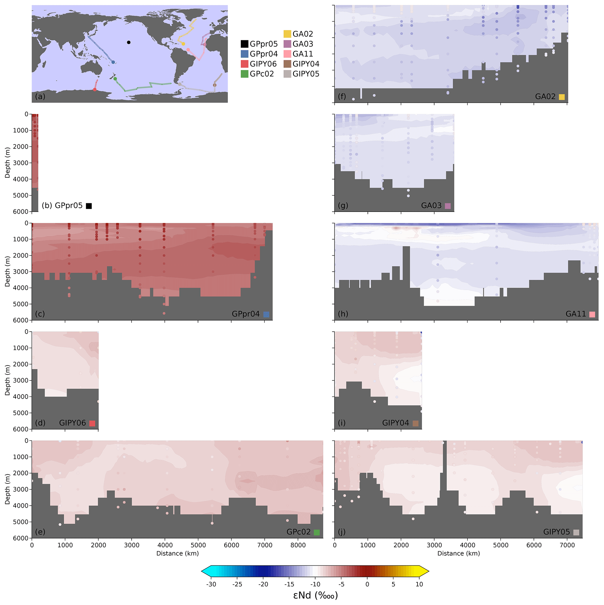
Figure 10(a) GEOTRACES cruise tracks with εNd observations. The legend layout matches the layout of the other subplots of the figure. (b–j) Modeled and observed εNd along GEOTRACES transects. Modeled values are shown as filled contours, while observed values are overlaid as a scatterplot.
Figure 11 shows the model and observed [Nd] and εNd for all observations averaged over different depth ranges. Contrary to Figs. 9 and 10, this includes all observations used to constrain the GNOM v1.0 (i.e., not just IDP17). As expected, the model broadly matches the observational data well, with some systematic mismatches in different locations. Figure 11d–e reveal an underestimate of deep [Nd] in the northern Indian Ocean in the Bay of Bengal, which is likely attributable to too strong scavenging or too weak sedimentary fluxes into the deeper layers of the model. Fig. 11c shows elevated Nd concentrations in the deepest parts of Baffin Bay, potentially due to too large sources, lack of data, or even circulation issues related to the resolution of the model grid in that region. Notably, Fig. 11c–e reveal discrepancies among observations, with a few [Nd] values near the GA02 transect that stand out compared to neighboring observations. Figure 11f–i show a substantial underestimate of equatorial Pacific εNd values above 1500 m depth, from east Indonesia to the west coast of Ecuador and Peru. Strongly negative observed εNd values in the northwestern Atlantic and near the west coast of Africa from the Congo River to Namibia are not well captured by the model. Conversely, rather positive εNd values at the surface going north along the western coast of North Africa also seem to evade the capability of GNOM to represent observations. The lack of resolution or some important missing mechanisms are likely the cause of these larger mismatches. In future versions of GNOM, we intend to improve the model by targeting these regions of particularly pronounced misfits.

Figure 11Model (heatmaps) and observations (markers) for (a–f) Nd concentrations and (g–k) εNd values. Model values are averaged over the indicated depth range. Individual observed values are overlaid on top of the modeled heatmap and on top of each other, so that perfect model–observation matches and deeper observations can be hard to see or hidden.
3.3 Diagnostics
One of the biggest advances in the GNOM v1.0, compared to earlier models of the marine Nd cycle, is due to the steady-state matrix formulation of the model, which allows us to compute advanced and detailed diagnostics that can directly address fundamental questions about the distribution of tracers and better understand their cycle. In the following sections, we showcase a few such diagnostics.
3.3.1 Source magnitudes
The optimized parameters determine the magnitude of the sources, which are collected in Table 3. In our best estimate, about 66 Mmol of Nd (or about 9500 metric tonnes) are injected into the global ocean every year. This falls slightly above the 38–57 Mmol yr−1 range of previous GCM models (see Table 1 for model references).
The eolian dust and sedimentary sources are the dominant ones contributing 24 and 32 Mmol yr−1 (about 35 % and 50 % of to total source), respectively. While this falls within the 0.69–60 Mmol yr−1 range for global eolian source magnitudes of previous modeling studies, our eolian sources are an order of magnitude larger than previous GCM-based modeling studies (0.69–3.5 Mmol yr−1; Table 1) and than the 4.4 Mmol yr−1 estimate of Greaves et al. (1994). This is likely due to our optimization procedure, during which Nd solubility is allowed to be adjusted within the whole 0 %–100 % range, compared to previous GCM-based studies that typically use a fixed 2 % solubility (Arsouze et al., 2009; Gu et al., 2019; Pöppelmeier et al., 2020). This is despite the initial guesses for βr values for dust set at 5 %, which penalizes large solubilities more than low solubilities (see the increased probability densities for low solubilities in Figs. B1a and B1b). The high optimized solubility of volcanic ash βvolc is also likely unrealistic, although the total contribution of volcanic ash is much smaller than mineral dust. We note that generally worse fits to [Nd] and εNd observations have been achieved with some of our optimization runs ending in distinct local minima with significantly smaller dust solubilities. (We do not show these worse mismatches, but we show the corresponding initial and final parameter values in Fig. B1.) Finally, we emphasize that it is not the goal of this work to establish estimates of the GNOM parameters and that we welcome future GNOM users to apply narrower ranges for those parameters for which they have better constraints (for example, restricting dust Nd solubilities to values below 10 %).
At 32 Mmol yr−1, the GNOM sedimentary source falls right within the 0–78 Mmol yr−1 range of previous models (28–55 Mmol yr−1 for GCM-based studies; Table 1) and in agreement with the 18–110 Mmol yr−1 range of Abbott et al. (2015b). The third-largest source is riverine, with about 10 Mmol yr−1, also in accord with the published 1.8–12.4 Mmol yr−1 range in previous models (Table 1) and similar to the 4.6–12 Mmol yr−1 values from Goldstein and Jacobsen (1987) and Greaves et al. (1994). The GNOM optimization did not favor a large source from submarine groundwater discharge, which has been estimated between 29–81 Mmol yr−1 by Johannesson and Burdige (2007), but this source was not included in any other modeling studies, so it is difficult to compare with other global model estimates. Hence, apart from a relatively elevated dust source, the GNOM optimization generally supports previous estimates of the magnitude of these sources.
Table 3Source magnitudes, their Nd contributions, and corresponding bulk residence time. Values are reported with two significant digits.
3.3.2 Partition according to source type
We partition Nd concentration according to source type simply by removing all the other sources. (The superposition principle applies directly to our model because it is linear in Nd; see, e.g., Holzer et al., 2016, who partitioned dissolved iron concentrations, first requiring the construction of a linear equivalent model.). With Ndk denoting neodymium that was injected by source type k, its corresponding column vector is thus computed by solving the following:
where . Taking the global volume-weighted mean of each gives the contribution of each source type to the total Nd inventory and are collected in Table 3.
As is the case for most global biogeochemical cycles, the relative source magnitudes and their relative contribution to the standing stock do not necessarily match. For instance, mineral dust, volcanic ash, and hydrothermal vents contribute more to the mean Nd concentration than their relative source magnitudes. These variations can be directly linked to the bulk residence time of Nd molecules, which vary with location of injection and consequently with source type.
3.3.3 Bulk residence times
The bulk residence time of Ndk is given by taking the ratio of its inventory to its source magnitude. Total Nd (i.e., from all sources) has a bulk residence time of roughly 440 years, which is within the 350–2900 year range of previous Nd cycling models. (The bulk residence time for GNOM falls slightly below the 560–750 year range of GCM-based models; see Table 1).
Unlike in the real ocean, where each molecule of Nd is indistinguishable from the next (with no information about its initial source), in a model we can track Nd coming from different sources and calculate source-partitioned residence times. We find that sedimentary-sourced Nd has the shortest residence time at 370 years. This is because it is injected just above the seafloor and is thus buried more quickly (i.e., a molecule of Nd sourced from the sediments at 5000 m, which only has to fall a few meters to be scavenged back to the sediments, leaves the ocean quicker than a molecule near the surface sourced from dust, which has to fall thousands of meters). In comparison, volcanic ash Nd, most of which is deposited onto the surface of the Pacific, remains on average 650 years in the system (i.e., about 75 % longer than sedimentary-sourced Nd). Mineral dust deposited Nd and riverine and surface groundwater Nd all show a residence time of about 550 years.
3.3.4 Tracking Nd to investigate εNd conservativeness
Sediment core records of εNd are of considerable importance for paleoceanography because they serve as a fingerprint of past ocean circulation and have been used, in particular, to infer changes in the Atlantic meridional overturning circulation (AMOC; e.g., Palmer and Elderfield, 1985; Rutberg et al., 2000; Piotrowski et al., 2004, 2005; van de Flierdt et al., 2006; Piotrowski et al., 2008; Pena et al., 2013; Pena and Goldstein, 2014; Huang et al., 2014; Kim et al., 2021; Pöppelmeier et al., 2021; Hines et al., 2022). Observations of modern ocean εNd have thus been extensively used to estimate Atlantic water mass fractions, typically inferred from north–south end-members and assuming quasi-conservative transport and mixing of εNd as an ocean circulation tracer (Hartman, 2015; Wu, 2019; Wu et al., 2022).
Our GNOM model – or, more precisely, the steady-state matrix schema with which it is built – allows for exact computations of these water masses and the contributions of various sources and regions to the modern ocean Nd and εNd distributions. We emphasize that by exact, here, we do not mean exact for the real ocean, but instead for our given choice of ocean circulation model (in this case the OCIM v2.0; DeVries and Holzer, 2019), which is arguably the best steady-state ocean circulation model available for such climatological estimates (see, e.g., John et al., 2020). Here, we merely showcase these diagnostics within GNOM, but in the future we plan to further explore the underlying scientific questions that these diagnostics can address.
We chose two simple regions that cover the entire ocean, except for the central Atlantic between 30∘ S and 40∘ N. We denote these regions by ΩN and ΩS, such that ΩN borders the northern Atlantic and ΩS the southern Atlantic. The regions are shown in Fig. 12.
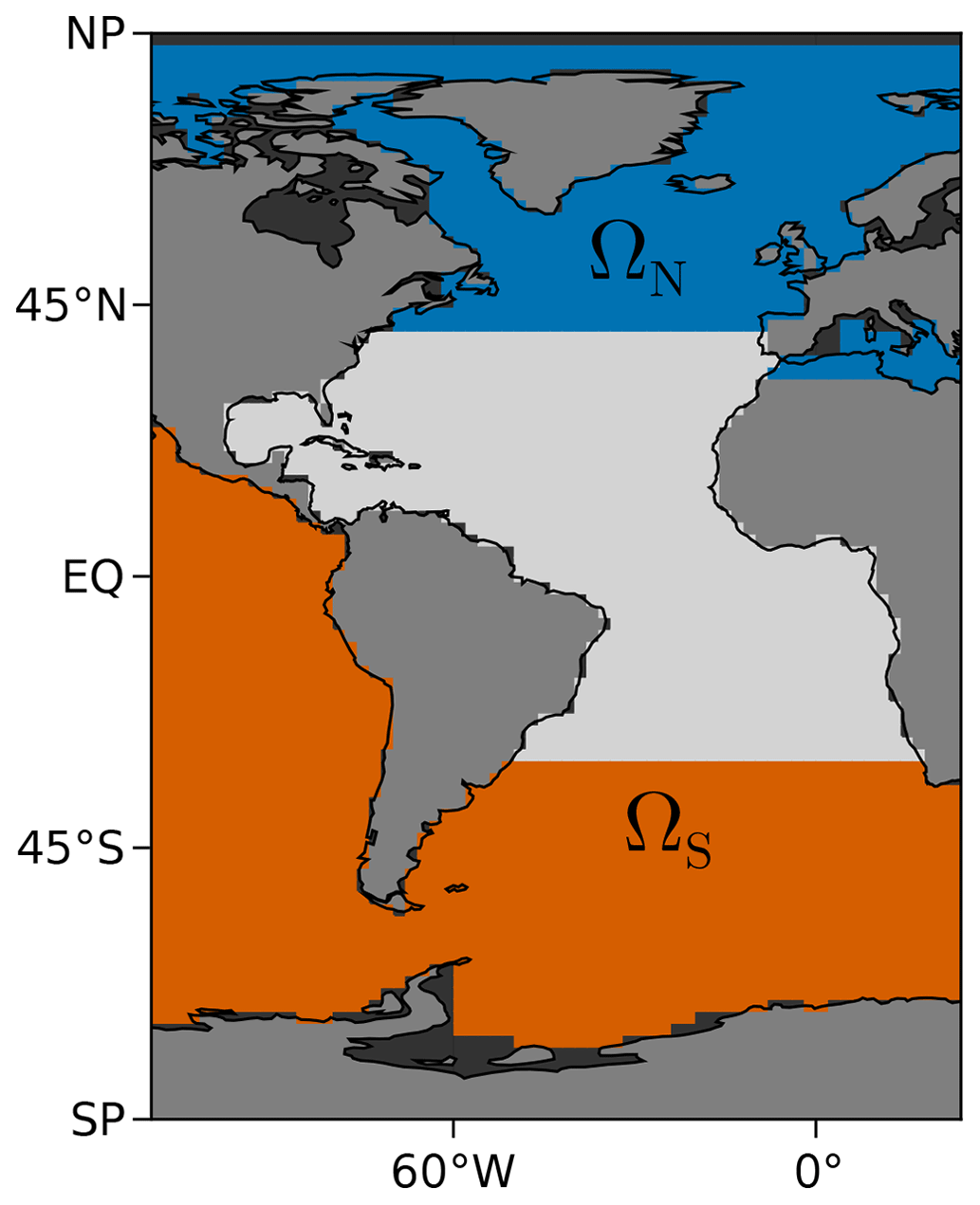
Figure 12Northern Atlantic (ΩN; blue) and southern Atlantic (ΩS; orange) regions used for the εNd conservativeness and the water-tagged Nd diagnostics within the central Atlantic region (from 30∘ S to 40∘ N; light gray).
First, we track Nd concentrations from each of these regions. Neodymium concentrations are not conservative, in part due to reversible scavenging and in part due to external sources that inject new Nd along transport pathways. For example, we can track Nd that came from region ΩN by tagging Nd that comes into contact with ΩN and removing that tag when Nd enters ΩS. Mathematically, we can perform this tagging/untagging by simulating a fictitious tracer, denoted NdN−tag, for which we enforce a concentration equal to simulated [Nd] in region ΩN, a concentration equal to zero in ΩS, and allowing reversible scavenging and burial to remove NdN−tag in between. In practice, we compute the corresponding column vector by solving the following:
where the Mi are diagonal matrices of which the diagonals are 1 s−1 for indices (i.e., coordinates) within the region Ωi and 0 s−1 otherwise. Because of the very short timescale of 1 s employed, Eq. (20) effectively enforces that pM in the region ΩS and that in the region ΩN (where [Nd] denotes the simulated concentration from the GNOM). We track NdS−tag in the same way by replacing MN with MS on the right-hand side of Eq. (20). The neodymium concentration that neither came from ΩN nor ΩS is then simply given by .
Figure 13 shows the Atlantic zonal averages of [NdN−tag], [NdS−tag], and non-tagged [Nd] (i.e., Nd that was injected in the central Atlantic between 30∘ S and 40∘ N). In the ΩN region (north of 40∘ N), 100 % of Nd is tagged as NdN−tag (Fig. 13a). Similarly, 100 % of Nd is NdS−tag in ΩS (Fig. 13b). Figure 13c shows the remaining non-tagged Nd and Fig. 13d combines Fig. 13a–c by showing only the dominant fraction. A clear signal of the influence of surface sources is visible down to about 1500 m, confining the dominance of the N- and S-tagged fractions of Nd to deep waters and to high latitudes, close to their respective tagging regions. In the future, we intend to further explore the extent of the influence of high latitudes on the distribution of Nd.
Gu et al. (2020) performed a north–south end-member partitioning using the CESM model and its POP2 circulation. They quantified water mass fractions using dye injections at the surface and compared them with water mass reconstructions from deep εNd values. Here we present more detailed partitions that have never been estimated in previous modeling studies to our knowledge.
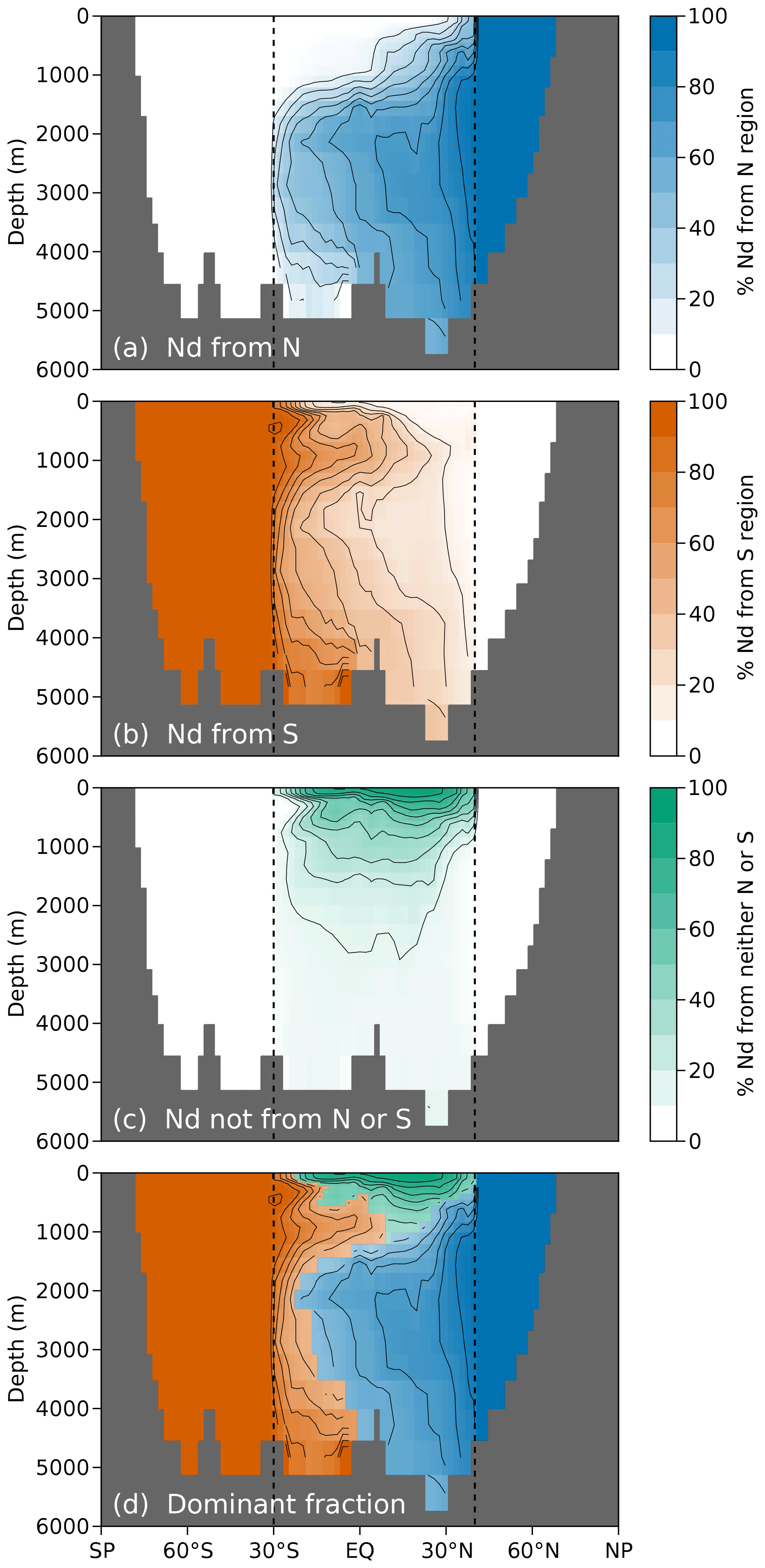
Figure 13(a) Atlantic zonal average of the fraction of Nd tagged in the ΩN region (north of 40∘ N; blue). (b) Same for Nd tagged in the ΩS region (south of 30∘ S; orange). (c) Same for Nd tagged injected within the midlatitude Atlantic (between 30∘ S and 40∘ N; green). (d) Atlantic zonal average showing only the dominant fraction of Nd coming from either ΩN or ΩS or from within 30∘ S–40∘ N. Contour lines are shown for each 10 % increment. Tagging regions are shown in Fig. 12.
We now track εNd, as if it were a conservative tracer, from the ΩN and ΩS regions. Technically, this is done by tracking water itself as it leaves either region. Water mass fractions estimated with this approach can be used to directly propagate modeled εNd values from the boundaries of the northern and southern Atlantic regions to provide an exact end-member mixing estimate that serves as a reference.
Water mass fractions have been estimated using a Green function boundary propagator in similar model contexts (e.g., Holzer and Hall, 2008; Primeau, 2005; Holzer and Primeau, 2008). They can be used to calculate the conservative transport of any tracer. As an illustrative example, here, we propagate modeled εNd simultaneously from both the ΩN and ΩS regions into the central Atlantic. This theoretical conservative value is denoted by (with Ω as a superscript to denote that its value is entirely determined by the εNd inside the ΩN and ΩS regions), and the corresponding column vector is computed by solving the following:
Like Eq. (20), Eq. (21) effectively enforces that matches modeled εNd inside ΩN and ΩS but is conservatively propagated by the advective–diffusive transport operator Tcirc outside of Ω. (Note the different operators on both the left-hand side and right-hand sides between Eqs. 20 and 21.)
Atlantic zonal averages of modeled εNd, conservatively propagated εNd, and their differences (Δ(εNd)) are shown in Fig. 14. Figure 14c, in particular, shows where εNd behaves conservatively (white), and where it does not (green or pink), in our model.
In accordance with Fig. 13, εNd is the least conservative close to the surface, where most of the Nd was never in contact with ΩS or ΩN and was instead injected in the midlatitude Atlantic. This surface overestimate is most pronounced away from ΩN and ΩS, with Δ(εNd) values of up to +10 ![]() .
Going from 200 to 1000 m depth, we find Δ(εNd) values decreasing from +5 to +1
.
Going from 200 to 1000 m depth, we find Δ(εNd) values decreasing from +5 to +1 ![]() .
Conservative εNd and true εNd remain within 1
.
Conservative εNd and true εNd remain within 1 ![]() of each other below 1000 m depth, despite a slight Δ(εNd) overestimate near the seafloor (likely due to the effect of local sedimentary flux) and a slight underestimate around 1500 m (potentially due to reversible scavenging). We intend to investigate the distinct conservativeness of Nd and εNd (the neodymium paradox) further in future work.
of each other below 1000 m depth, despite a slight Δ(εNd) overestimate near the seafloor (likely due to the effect of local sedimentary flux) and a slight underestimate around 1500 m (potentially due to reversible scavenging). We intend to investigate the distinct conservativeness of Nd and εNd (the neodymium paradox) further in future work.

The most prominent caveat of GNOM v1.0 is the steady-state assumption, which we apply to both the circulation and the Nd cycle. Hence, by construction, daily, seasonal, decadal, or multi-decadal fluctuations that deviate from the climatological mean cannot be captured by our model. However, we trust that the circulation model used (the OCIM v2.0; DeVries and Holzer, 2019), which is data-assimilated with ventilation tracers, captures the predominant features and pathways of the modern ocean circulation and provides the most realistic steady-state transport to date (e.g., DeVries and Holzer, 2019; John et al., 2020).
We note that, compared to previous modeling studies, the GNOM does not represent scavenging by calcium carbonate (CaCO3) because there is no publicly available particulate CaCO3 field, to the best of our knowledge. Modeling scavenging is a challenging task that the GNOM model does not pretend to achieve with high accuracy. However, we deem the current implementation satisfactory, considering the quality of the overall model–observation fit. Future versions of the GNOM could include CaCO3 particle scavenging or a generally improved scavenging parameterization.
Our model reveals some locations of particular interest for improving our understanding of the Nd cycle and εNd patterns. For instance, there are only two GEOTRACES transects in the Pacific Ocean which cover the western Pacific and the Southern Ocean, the zonal transects in the Atlantic contain only a few εNd measurements compared to [Nd] (e.g., GA03, GA10, GA11, and GAc01), and there are no published transects in the Indian Ocean, which may contribute a non-negligible fraction of Nd to both the Atlantic and Pacific. In the future, we hope that more data will be made available and improve the capabilities of data-constrained model estimates of εNd and the Nd cycle.
While our model endeavors to use formulations and parameter constraints which have reasonable biogeochemical interpretations, there is always room for improvement. For example, our sedimentary source parameterization, which we plan to investigate further in future work, assumes an exponential profile for the sedimentary source flux. While this parameterization is flexible enough to reproduce most of the qualitative features of the sedimentary fluxes in previous models, one might argue that a more mechanistic model of the sedimentary budget would result in a more realistic overall Nd cycling model.
Despite the theoretical advantages they confer to the convergence rate of our optimization procedure, our specific choice of prior distributions for the parameters (Fig. B1) remains arbitrary, though the ranges chosen are of course informed by prior work. Different ranges and initial conditions would yield different optimal solutions and therefore different parameter values. Our choice of a local Newton trust region optimizer also exposes our strategy to the risk of getting stuck in local minima. To counter that risk, we have opted for the traditional ad hoc countermeasure of running the optimization from multiple, randomized initial guesses. While this offers the advantage of spanning a large number of cases, it offers no guarantees that the optimal set of parameters represents a global minimum. It is thus entirely likely that a better set of parameter values would reduce the objective function value and improve the model skill, though again we note that the most important features of Nd biogeochemical cycling are likely to converge to similar values regardless of initial conditions.
Our specific choice of objective function gives a measure of the skill of the model for reproducing [Nd] and εNd observations. Roughly speaking, despite our arbitrary choices for the weights ωNd, , and ωp involved in Eq. (17), the value of the objective function can also be interpreted as the negative log-likelihood of observing the measured εNd and [Nd], given the model and its parameters. In the future, we plan to determine the values of hyperparameters, such as ωNd, , and ωp through a more formal Bayesian approach.
Qualitatively, GNOM compares well to previous models that are embedded in ocean general circulation models and simulate two explicit Nd isotopes (Arsouze et al., 2009; Rempfer et al., 2011; Gu et al., 2019; Pöppelmeier et al., 2020). Given that these models were built with a different objective, less available data, and without a systematic optimization of all parameters, we expect GNOM v1.0 to perform better against the objective function used in this study. However, we emphasize that these previous models are more suited to specific experiments, including simulations of transient changes in circulation on millennial timescales. In other words, these previous models are not all restricted by the caveats of a coarse steady-state circulation. We also note that the underlying circulation used in GNOM can be swapped with any other circulation available through the AIBECS.jl framework (see Pasquier et al., 2022b), although we reiterate that the OCIM v2.0 likely offers the best available representation of the current ocean circulation.
The main advantages of the GNOM are skill and computational efficiency. The GNOM v1.0 owes its low computational cost and quick simulation time to the steady-state OCIM v2.0 circulation in which it is embedded and the linear representation that allows us to solve the system of tracer equations in a single matrix inversion. The model's skill comes from the optimization procedure and likely benefits from the quality of the OCIM v2.0 circulation. The GNOM is also versatile in many respects owing to its simplicity. Parameter values and acceptable ranges can be tuned, entire mechanisms can be turned off, eliminating free parameters, or added with a few changes of simple lines of code. This versatility is compounded by computational speed, which makes GNOM ideally suited for quick experimentation and further optimization. The GNOM model is also easily diagnosed, owing to the powerful tools of linear algebra. Novel diagnostics offer new insights by revealing features often hidden in standard model output. Finally, as it is available in a self-contained package (except for the GEOTRACES dataset, which is not programmatically accessible), the GNOM v1.0 offers unprecedented reproducibility, which is sorely lacking in advanced research (Peng, 2011; Irving, 2016). Thanks to the advantages listed above, the GNOM is well positioned for answering long-lasting questions and exploring new ideas about the Nd cycle and the εNd distributions.
To represent scavenging by opal (particulate silica), we designed and optimize a simple Si cycling model in parallel to our Nd cycling model. Our Si cycling model is a simple nutrient restoring model embedded in the same OCIM v2.0 circulation. We emphasize that the goal here is only to generate a reasonable 3D field for particulate biogenic silica concentrations.
The Si cycling model considered here explicitly tracks two tracers, DSi and PSi. We thus denote the modeled column vectors for DSi and PSi concentrations by the following: , and . Biological uptake of silicate in the euphotic zone is essentially modeled after the simple nutrient restoring scheme of the OCIMP-2 protocol (Najjar et al., 2007) with some slight modification. Specifically, the uptake rate vector is defined by the following:
where (z<z0) ensures that uptake only happens in the euphotic zone, and is the modified nutrient-restoring scheme. Technically, (z<z0) is an abuse of notation and is here meant to be equal to 1 in the euphotic zone and 0 otherwise (z is the column vector depths and z0=80 m is the depth of the base of the euphotic zone). The column vector represents World Ocean Atlas silicate observations (WOA18; Garcia et al., 2019) regridded to the OCIM v2.0 grid. Here, (x)+ is a shortcut notation for x(x>0), such that only activates when . The difference with the standard Ocean Carbon-cycle Model Intercomparison Project (OCMIP-2) protocol lies in the addition of the αup modifier, which is a scalar that scales the field of observed silicate, allowing the optimized model to better fit observations. With αup close to 1, this parameterization essentially allows for the model to take up silicate in the euphotic zone when the simulated DSi concentration exceeds the observations.
All the silicate that is taken up in this model is converted to sinking particulate PSi, which gravitationally settles with optimizable velocity parameter wSi. Particulate biogenic silica is assumed to remineralize and redissolve into DSi in the water column with an optimizable timescale τrem. The rate of remineralization, , is thus simply defined by the following:
which essentially closes the Si cycle.
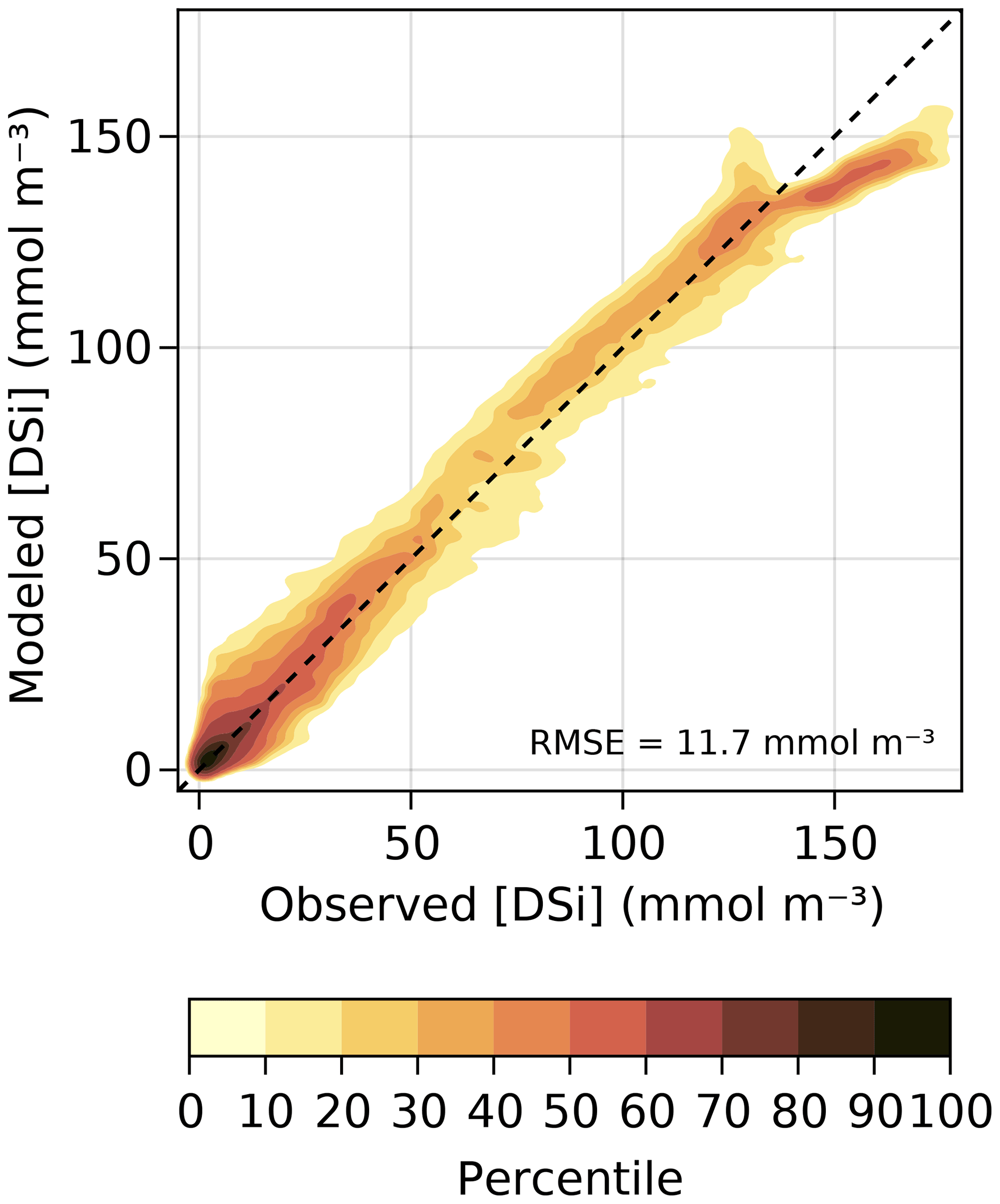
Figure A1Quantiles of the cumulative joint probability density functions of modeled and observed dissolved Si concentrations for the parallel Si cycling model. Darker colors indicate high density of data, such that n % of the modeled and observed data lie outside of the nth percentile contour. The closer the darker contours are to the 1:1 black dashed line, the better the fit.
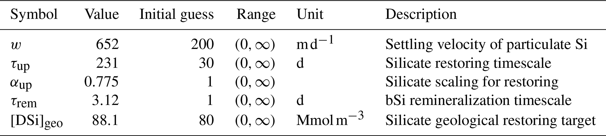
Hence, the steady-state tracer equation for dissolved silicate (DSi) is as follows:
where is an added term used to constrain the global inventory of Si in the system, which is set on geological timescales. In practice, we use the following:
where [DSi]geo is the optimizable global mean DSi concentration to which DSi concentrations are restored to with the timescale τgeo=1 Myr. Conversely, the connected steady-state tracer equation for particulate biogenic silica (PSi) is as follows:
where Tgrav is the vertical (downward) transport operator representing the flux divergence of particles. Particulate Si reaching the seafloor is not buried and instead remains in the deepest grid cell until eventual remineralization and redissolution into DSi.
A similar optimization procedure as for the Nd cycle is applied to optimize the five parameters collected in Table A1. The joint probability distribution of the mismatch between modeled and observed silicate is shown in Fig. A1. While not perfect overall, this simple model achieves a good fit to observations with a root mean square error of about 11.7 Mmol m−3.
Figure B1 shows the prior distributions and optimized values of the parameters listed in Table 2.
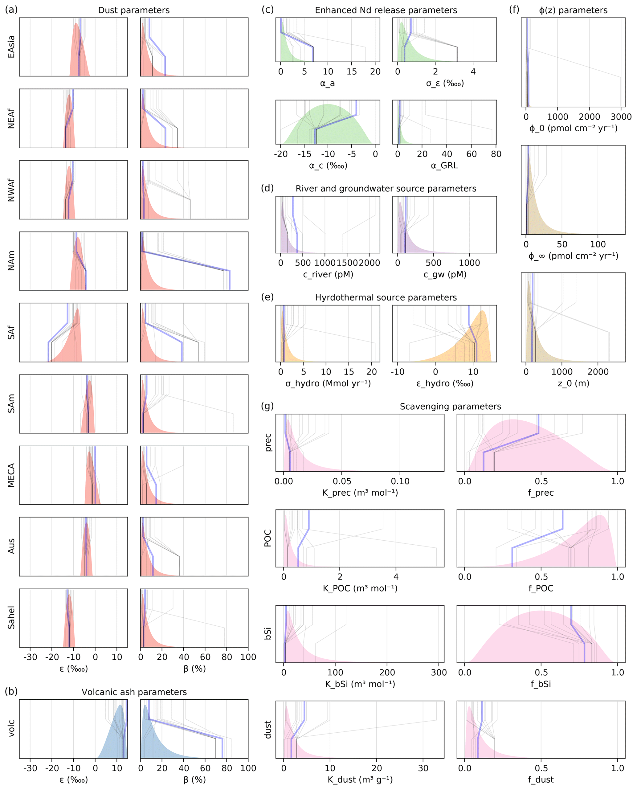
Figure B1Parameter prior distributions (color-filled densities) and initial and optimized parameter values for a dozen of optimization runs (lines). Each line starts by showing the initial parameter value at the top and is connected to the final optimized value at the bottom. The thicker blue line represents the optimization run that was used as our best estimate. (a) Dust εNd values (εr) and solubilities (βr) for each region of origin r. (b) Volcanic ash εNd value (εvolc) and solubility (βvolc). (c) Enhanced Nd release parameters, α curve parameters (curvature αa and center αc), Greenland enhancement (αGRL), and global standard deviation of per-grid-cell in situ sedimentary εNd (σε). (d) Rivers and groundwater Nd concentrations (criver and cgw). (e) Global hydrothermal source magnitude (σhydro) and εNd (εhydro). (f) Sedimentary flux parameters (ϕ0, ϕ∞, and z0). (g) Reversible scavenging reaction equilibrium constants, KX, and fractions returned to water when reaching seafloor, fX, for each particle type X. See also Table 2.
This appendix describes the effect that enhanced Nd release with extreme εNd values has on effectively released εNd. Let X be a random variable with the normal distribution 𝒩(με,σε) denoting the observable in situ εNd value, and let Y denote the random variable of the effectively released εNd value. The mean expected value for Y is given by the following:
where α is defined in Eq. (8).
From the moments of a normal distribution, one can show, in the following, that:
and, in the following, that:
so that, in the following:
The GNOM model code is open source and publicly available for free. An archive of the GNOM v1.0.2 code used in this study is hosted permanently on Zenodo at https://doi.org/10.5281/zenodo.6118414 (Pasquier et al., 2022a). New developments are also available directly on GitHub at https://github.com/MTEL-USC/GNOM (last access: 26 May 2022). All the dependencies are free and open source and are version controlled through the GNOM project manifest file.
The code is written in Julia, which is itself free and open source (Bezanson et al., 2017). The Julia version that was used for this study is v1.6.2.
The GNOM v1 model was designed using the open-source AIBECS framework, available as a Julia package (Pasquier, 2020a; Pasquier et al., 2022b) at https://github.com/JuliaOcean/AIBECS.jl (last access: 26 May 2022).
Except for the GEOTRACES IDP17 data, which must be downloaded manually (see http://www.geotraces.org, last access: 26 May 2022), the entirety of the data used in this study can be programmatically downloaded by the GNOM code (also explained in the GNOM documentation) and are all available through the AIBECS.jl interface (Pasquier, 2020a; Pasquier et al., 2022b). These include the following:
-
the OCIM v2.0 circulations by DeVries and Holzer (2019) (with original files available at https://tdevries.eri.ucsb.edu/models-and-data-products/, last access: 26 May 2022),
-
the two-dimensional dust deposition fields partitioned according to region of origin from Kok et al. (2021a) and Kok et al. (2021b) (original files available from Adebiyi et al., 2020),
-
the aerosol-type partitioned dust source that includes volcanic ash as used by Chien et al. (2016) and Brahney et al. (2015) (original files available from http://www.geo.cornell.edu/eas/PeoplePlaces/Faculty/mahowald/dust/Chienetal2016/, last access: 26 May 2022),
-
the riverine discharge dataset from Dai and Trenberth (2002) (original files available from Dai, 2017),
-
the groundwater discharge from coastal sheds dataset compilation from Luijendijk et al. (2020) (with original files available from Luijendijk et al., 2019),
-
the hydrothermal 3He mantle source from the OCIM v2.0 product of DeVries and Holzer (2019) (original files available at https://tdevries.eri.ucsb.edu/models-and-data-products/, last access: 26 May 2022), and
-
the particulate organic carbon three-dimensional fields from Weber et al. (2018).
The three-dimensional field for biogenic opal particles described in Appendix A is entirely generated by a parallel inverse model of the Si cycle embedded in the GNOM code. The World Ocean Atlas silicate data (Garcia et al., 2019) used to constrain the parallel Si cycle can be downloaded programmatically by the WorldOceanAtlasTools.jl package and is available at https://data.nodc.noaa.gov/woa/ (last access: 26 May 2022).
The pre-GEOTRACES IDP17 historical dataset for Nd and εNd from van de Flierdt et al. (2016a) is available at https://doi.org/10.6084/m9.figshare.3980064.v1 (van de Flierdt et al., 2016b), and the post-IDP17 data compiled for this study are available at https://doi.org/10.6084/m9.figshare.15058329.v1 (Pasquier, 2021), both of which are also downloadable programmatically by the GNOM code.
Except for the model schematic (Fig. 1) that was created with TikZ (Tantau et al., 2013), all the figures in this paper were created using the Makie.jl package (https://github.com/JuliaPlots/Makie.jl, last access: 26 May 2022) (Danisch et al., 2021; Danisch and Krumbiegel, 2021). (All the plotting scripts are available in the GNOM repository at https://github.com/MTEL-USC/GNOM/, last access: 26 May 2022, and in the GNOM v1.0.2 Zenodo archive at https://doi.org/10.5281/zenodo.6118414, Pasquier et al., 2022a.)
SKVH, BP, SLG, and SGJ designed the study. HL wrote preliminary MATLAB code. BP wrote the Julia model code, performed simulations, and analyzed the data, with input from all authors. SKVH and BP wrote the original draft, and all authors contributed to revision and editing of the paper prior to submission.
The contact author has declared that neither they nor their co-authors have any competing interests.
Publisher's note: Copernicus Publications remains neutral with regard to jurisdictional claims in published maps and institutional affiliations.
The authors would like to thank Brian Haley, two other anonymous reviewers, and the editor, for their helpful comments which substantially improved this paper.
This work has been supported by the Simons Foundation (grant no. 426570SP to Seth G. John), the National Science Foundation (grant no. OCE-1736896 to Seth G. John and grant no. OCE-1831415 to Steven L. Goldstein and Sophia K. V. Hines), the Investment in Science Fund at WHOI and the John E. and Anne W. Sawyer Endowed Fund in Support of Scientific Staff (Sophia K. V. Hines), and the Storke Endowment of the Department of Earth and Environmental Sciences, Columbia University (Steven L. Goldstein).
This paper was edited by Andrew Yool and reviewed by Brian Haley and two anonymous referees.
Abbott, A. N., Haley, B. A., and McManus, J.: Bottoms up: Sedimentary control of the deep North Pacific Ocean's εNd signature, Geology, 43, 1035–1035, https://doi.org/10.1130/g37114.1, 2015a. a
Abbott, A. N., Haley, B. A., McManus, J., and Reimers, C. E.: The sedimentary flux of dissolved rare earth elements to the ocean, Geochim. Cosmochim. Ac., 154, 186–200, https://doi.org/10.1016/j.gca.2015.01.010, 2015b. a, b
Adebiyi, A. A., Kok, J. F., Wang, Y., Ito, A., Ridley, D. A., Nabat, P., and Zhao, C.: Dust Constraints from joint Observational-Modelling-experiMental analysis (DustCOMM): comparison with measurements and model simulations, Atmos. Chem. Phys., 20, 829–863, https://doi.org/10.5194/acp-20-829-2020, 2020. a, b, c, d
Adkins, J. F.: The role of deep ocean circulation in setting glacial climates, Paleoceanography, 28, 539–561, https://doi.org/10.1002/palo.20046, 2013. a
Amakawa, H., Yu, T.-L., Tazoe, H., Obata, H., Gamo, T., Sano, Y., Shen, C.-C., and Suzuki, K.: Neodymium concentration and isotopic composition distributions in the southwestern Indian Ocean and the Indian sector of the Southern Ocean, Chem. Geol., 511, 190–203, https://doi.org/10.1016/j.chemgeo.2019.01.007, 2019. a
Anderson, S. P.: Glaciers show direct linkage between erosion rate and chemical weathering fluxes, Geomorphology, 67, 147–157, https://doi.org/10.1016/j.geomorph.2004.07.010, 2005. a
Arsouze, T., Dutay, J.-C., Lacan, F., and Jeandel, C.: Modeling the neodymium isotopic composition with a global ocean circulation model, Chem. Geol., 239, 165–177, https://doi.org/10.1016/j.chemgeo.2006.12.006, 2007. a, b
Arsouze, T., Dutay, J.-C., Lacan, F., and Jeandel, C.: Reconstructing the Nd oceanic cycle using a coupled dynamical – biogeochemical model, Biogeosciences, 6, 2829–2846, https://doi.org/10.5194/bg-6-2829-2009, 2009. a, b, c, d, e
Arsouze, T., Treguier, A. M., Peronne, S., Dutay, J.-C., Lacan, F., and Jeandel, C.: Modeling the Nd isotopic composition in the North Atlantic basin using an eddy-permitting model, Ocean Sci., 6, 789–797, https://doi.org/10.5194/os-6-789-2010, 2010. a, b
Bacon, M. P. and Anderson, R. F.: Distribution of thorium isotopes between dissolved and particulate forms in the deep sea, J. Geophys. Res.-Oceans, 87, 2045–2056, https://doi.org/10.1029/JC087iC03p02045, 1982. a
Basak, C., Pahnke, K., Frank, M., Lamy, F., and Gersonde, R.: Neodymium isotopic characterization of Ross Sea Bottom Water and its advection through the southern South Pacific, Earth Planet. Sc. Lett., 419, 211–221, https://doi.org/10.1016/j.epsl.2015.03.011, 2015. a
Behrens, M. K., Pahnke, K., Paffrath, R., Schnetger, B., and Brumsack, H.-J.: Rare earth element distributions in the West Pacific: Trace element sources and conservative vs. non-conservative behavior, Earth Planet. Sc. Lett., 486, 166–177, https://doi.org/10.1016/j.epsl.2018.01.016, 2018a. a
Behrens, M. K., Pahnke, K., Schnetger, B., and Brumsack, H.-J.: Sources and processes affecting the distribution of dissolved Nd isotopes and concentrations in the West Pacific, Geochim. Cosmochim. Ac., 222, 508–534, https://doi.org/10.1016/j.gca.2017.11.008, 2018b. a
Bertram, C. and Elderfield, H.: The geochemical balance of the rare earth elements and neodymium isotopes in the oceans, Geochim. Cosmochim. Ac., 57, 1957–1986, https://doi.org/10.1016/0016-7037(93)90087-D, 1993. a, b, c
Bezanson, J., Edelman, A., Karpinski, S., and Shah, V. B.: Julia: A Fresh Approach to Numerical Computing, SIAM Review, 59, 65–98, https://doi.org/10.1137/141000671, 2017. a, b
Blaser, P., Lippold, J., Gutjahr, M., Frank, N., Link, J. M., and Frank, M.: Extracting foraminiferal seawater Nd isotope signatures from bulk deep sea sediment by chemical leaching, Chem. Geol., 439, 189 – 204, https://doi.org/10.1016/j.chemgeo.2016.06.024, 2016. a, b, c
Blaser, P., Gutjahr, M., Pöppelmeier, F., Frank, M., Kaboth-Bahr, S., and Lippold, J.: Labrador Sea bottom water provenance and REE exchange during the past 35,000 years, Earth Planet. Sc. Lett., 542, 116299, https://doi.org/10.1016/j.epsl.2020.116299, 2020. a, b
Bouvier, A., Vervoort, J. D., and Patchett, P. J.: The Lu–Hf and Sm–Nd isotopic composition of CHUR: Constraints from unequilibrated chondrites and implications for the bulk composition of terrestrial planets, Earth Planet. Sc. Lett., 273, 48–57, https://doi.org/10.1016/j.epsl.2008.06.010, 2008. a
Brahney, J., Mahowald, N., Ward, D. S., Ballantyne, A. P., and Neff, J. C.: Is atmospheric phosphorus pollution altering global alpine Lake stoichiometry?, Global Biogeochem. Cycles, 29, 1369–1383, https://doi.org/10.1002/2015GB005137, 2015. a, b
Byrne, R. H. and Kim, K.-H.: Rare earth element scavenging in seawater, Geochim. Cosmochim. Ac., 54, 2645–2656, https://doi.org/10.1016/0016-7037(90)90002-3, 1990. a
Che, H. and Zhang, J.: Water Mass Analysis and End-Member Mixing Contribution Using Coupled Radiogenic Nd Isotopes and Nd Concentrations: Interaction Between Marginal Seas and the Northwestern Pacific, Geophys. Res. Lett., 45, 2388–2395, https://doi.org/10.1002/2017GL076978, 2018. a
Chien, C.-T., Mackey, K. R. M., Dutkiewicz, S., Mahowald, N. M., Prospero, J. M., and Paytan, A.: Effects of African dust deposition on phytoplankton in the western tropical Atlantic Ocean off Barbados, Global Biogeochem. Cycles, 30, 716–734, https://doi.org/10.1002/2015GB005334, 2016. a, b, c
Dai, A.: Historical and Future Changes in Streamflow and Continental Runoff, chap. 2, 17–37, American Geophysical Union (AGU), https://doi.org/10.1002/9781118971772.ch2, 2016. a
Dai, A.: Dai and Trenberth Global River Flow and Continental Discharge Dataset, Research Data Archive at the National Center for Atmospheric Research, Computational and Information Systems Laboratory, https://doi.org/10.5065/D6V69H1T, 2017. a, b, c
Dai, A. and Trenberth, K. E.: Estimates of Freshwater Discharge from Continents: Latitudinal and Seasonal Variations, J. Hydrometeorol., 3, 660–687, https://doi.org/10.1175/1525-7541(2002)003<0660:EOFDFC>2.0.CO;2, 2002. a, b
Dai, A., Qian, T., Trenberth, K. E., and Milliman, J. D.: Changes in Continental Freshwater Discharge from 1948 to 2004, J. Climate, 22, 2773–2792, https://doi.org/10.1175/2008JCLI2592.1, 2009. a
Danisch, S. and Krumbiegel, J.: Makie.jl: Flexible high-performance data visualization for Julia, J. Open Source Softw., 6, 3349, https://doi.org/10.21105/joss.03349, 2021. a
Danisch, S., Krumbiegel, J., Singhvi, A., Freyer, F., Wang, A., Vertechi, P., Holy, T., Widmann, D., Krabbe Borregaard, M., Datseris, G., M. M., Greimel, F., Butterworth, I., Foster, C., Dehaybe, H., Schauer, M., Kilpatrick, L., Byrne, S., kragol, Weidner, J., Hatherly, M., Sharma, A., Micluța-Câmpeanu, S., t-bltg, Herikstad, R., Goretkin, G., TagBot, J., Štih, V., and smldis: JuliaPlots/Makie.jl, Zenodo, https://doi.org/10.5281/zenodo.3735092, 2021. a
Dausmann, V., Frank, M., and Zieringer, M.: Dissolved Hafnium and Neodymium data measured on water samples during METEOR cruise M84/5 in the Bay of Biscay, PANGAEA, https://doi.org/10.1594/PANGAEA.902808, 2019. a
Dausmann, V., Frank, M., and Zieringer, M.: Water mass mixing versus local weathering inputs along the Bay of Biscay: Evidence from dissolved hafnium and neodymium isotopes, Marine Chemistry, 224, 103844, https://doi.org/10.1016/j.marchem.2020.103844, 2020. a
de Baar, H. J. W., Bacon, M. P., and Brewer, P. G.: Rare-earth distributions with a positive Ce anomaly in the Western North Atlantic Ocean, Nature, 310, 324–327, https://doi.org/10.1038/301324a0, 1983. a
de Baar, H. J. W., Bacon, M. P., Brewer, P. G., and Bruland, K. W.: Rare earth elements in the Pacific and Atlantic Oceans, Geochim. Cosmochim. Ac., 49, 1943–1959, https://doi.org/10.1016/0016-7037(85)90089-4, 1985. a
DePaolo, D. J. and Wasserburg, G. J.: Nd isotopic variations and petrogenetic models, Geophys. Res. Lett., 3, 249–252, https://doi.org/10.1029/GL003i005p00249, 1976. a, b, c
Dessert, C., Dupré, B., Gaillardet, J., François, L. M., and Allègre, C. J.: Basalt weathering laws and the impact of basalt weathering on the global carbon cycle, Chem. Geol., 202, 257–273, https://doi.org/10.1016/j.chemgeo.2002.10.001, 2003. a
DeVries, T.: The oceanic anthropogenic CO2 sink: Storage, air–sea fluxes, and transports over the industrial era, Global Biogeochem. Cycles, 28, 631–647, https://doi.org/10.1002/2013GB004739, 2014. a, b
DeVries, T. and Holzer, M.: Radiocarbon and Helium Isotope Constraints on Deep Ocean Ventilation and Mantle-3He Sources, J. Geophys. Res.-Oceans, 124, 3036–3057, https://doi.org/10.1029/2018JC014716, 2019. a, b, c, d, e, f, g, h, i, j
DeVries, T. and Primeau, F.: Dynamically and Observationally Constrained Estimates of Water-Mass Distributions and Ages in the Global Ocean, J. Phys. Oceanogr., 41, 2381–2401, https://doi.org/10.1175/JPO-D-10-05011.1, 2011. a, b
Du, J., Haley, B. A., and Mix, A. C.: Neodymium isotopes in authigenic phases, bottom waters and detrital sediments in the Gulf of Alaska and their implications for paleo-circulation reconstruction, Geochim. Cosmochim. Ac., 193, 14–35, 2016. a, b
Du, J., Haley, B. A., and Mix, A. C.: Evolution of the Global Overturning Circulation since the Last Glacial Maximum based on marine authigenic neodymium isotopes, Quaternary Sci. Rev., 241, 106396, https://doi.org/10.1016/j.quascirev.2020.106396, 2020. a, b, c, d
Elderfield, H.: The oceanic chemistry of the rare-earth elements, Philos. T. Roy. Soc. Lond. A, 325, 105–126, https://doi.org/10.1098/rsta.1988.0046, 1988. a, b
Elderfield, H. and Greaves, M. J.: The rare earth elements in seawater, Nature, 296, 214–219, https://doi.org/10.1038/296214a0, 1982. a
Elderfield, H. and Sholkovitz, E. R.: Rare earth elements in the pore waters of reducing nearshore sediments, Earth Planet. Sc. Lett., 82, 280–288, https://doi.org/10.1016/0012-821x(87)90202-0, 1987. a, b, c
Elderfield, H., Hawkesworth, C. J., Greaves, M. J., and Calvert, S. E.: Rare earth element geochemistry of oceanic ferromanganese nodules and associated sediments, Geochim. Cosmochim. Ac., 45, 513–528, https://doi.org/10.1016/0016-7037(81)90184-8, 1981. a, b
Frank, M.: Radiogenic isotopes: Tracers of past ocean circulation and erosional input, Rev. Geophys., 40, 1-1–1-38, https://doi.org/10.1029/2000RG000094, 2002. a, b, c
Fröllje, H., Pahnke, K., Schnetger, B., Brumsack, H.-J., Dulai, H., and Fitzsimmons, J. N.: Hawaiian imprint on dissolved Nd and Ra isotopes and rare earth elements in the central North Pacific: Local survey and seasonal variability, Geochim. Cosmochim. Ac., 189, 110–131, https://doi.org/10.1016/j.gca.2016.06.001, 2016. a
Gaillardet, J., Dupré, B., Louvat, P., and Allègre, C.: Global silicate weathering and CO2 consumption rates deduced from the chemistry of large rivers, Chem. Geol., 159, 3–30, https://doi.org/10.1016/S0009-2541(99)00031-5, 1999. a
Garcia, H. E., Weathers, K., Paver, C. R., Smolyar, I., Boyer, T. P., Locarnini, R. A., Zweng, M. M., Mishonov, A. V., Baranova, O. K., Seidov, D., and Reagan, J. R.: World Ocean Atlas 2018, NOAA Atlas NESDIS 84, vol. 4: Dissolved Inorganic Nutrients (phosphate, nitrate and nitrate+nitrite, silicate), edited by: Mishonov, A., NOAA Atlas NESDIS 84, 35 pp., 2019. a, b
Garcia-Solsona, E., Jeandel, C., Labatut, M., Lacan, F., Vance, D., Chavagnac, V., and Pradoux, C.: Rare earth elements and Nd isotopes tracing water mass mixing and particle-seawater interactions in the SE Atlantic, Geochim. Cosmochim. Ac., 125, 351–372, https://doi.org/10.1016/j.gca.2013.10.009, 2014. a, b
Gardner, W. D., Richardson, M. J., and Mishonov, A. V.: Global assessment of benthic nepheloid layers and linkage with upper ocean dynamics, Earth Planet. Sc. Lett., 482, 126–134, https://doi.org/10.1016/j.epsl.2017.11.008, 2018. a
Gebbie, G. and Huybers, P. J.: Total Matrix Intercomparison: A Method for Determining the Geometry of Water-Mass Pathways, J. Phys. Oceanogr., 40, 1710–1728, https://doi.org/10.1175/2010JPO4272.1, 2010. a
GEOTRACES Planning Group: GEOTRACES Science Plan, Baltimore, Maryland, Scientific Committee on Oceanic Research, https://geotracesold.sedoo.fr/libraries/documents/Science_plan.pdf (last access: 7 June 2022), 2006. a
German, C. R., Masuzawa, T., Greaves, M. J., Elderfield, H., and Edmond, J. M.: Dissolved Rare Earth Elements in the Southern Ocean: golCerium Oxidation and the Influence of Hydrography, Geochim. Cosmochim. Ac., 59, 1551–1558, https://doi.org/10.1016/0016-7037(95)00061-4, 1995. a
Goldberg, E. D., Koide, M., Schmitt, R. A., and Smith, R. H.: Rare-Earth Distributions in the Marine Environment, J. Geophys. Res., 68, 4209–4217, https://doi.org/10.1029/JZ068i014p04209, 1963. a
Goldstein, S. and Hemming, S. R.: Long-lived isotopic tracers in oceanography, paleoceanography, and ice-sheet dynamics, in: Treatise on Geochemistry, edited by: Holland, H. D. and Turekian, K. K., 453–489, Pergamon, Oxford, https://doi.org/10.1016/B0-08-043751-6/06179-X, 2003. a, b, c, d
Goldstein, S. and O'Nions, R. K.: Nd and Sr Isotopic Relationships in Pelagic Clays and Ferromanganese Deposits, Nature, 292, 324–327, https://doi.org/10.1038/292324a0, 1981. a, b
Goldstein, S. L. and Jacobsen, S. B.: The Nd and Sr Isotopic Systematics of River-Water Dissolved Material: Implications for the Sources of Nd and Sr in Seawater, Chem. Geol., 66, 245–272, 1987. a
Goldstein, S. L., O'Nions, R. K., and Hamilton, P. J.: A Sm–Nd isotopic study of atomospheric dusts and particulates from major river system, Earth Planet. Sc. Lett., 70, 221–236, https://doi.org/10.1016/0012-821X(84)90007-4, 1984. a, b, c, d
Greaves, M., Statham, P., and Elderfield, H.: Rare earth element mobilization from marine atmospheric dust into seawater, Marine Chemistry, 46, 255–260, https://doi.org/10.1016/0304-4203(94)90081-7, 1994. a, b
Grenier, M., Garcia-Solsona, E., Lemaitre, N., Trull, T. W., Bouvier, V., Nonnotte, P., van Beek, P., Souhaut, M., Lacan, F., and Jeandel, C.: Differentiating Lithogenic Supplies, Water Mass Transport, and Biological Processes On and Off the Kerguelen Plateau Using Rare Earth Element Concentrations and Neodymium Isotopic Compositions, Front. Marine Sci., 5, 426, https://doi.org/10.3389/fmars.2018.00426, 2018. a
Gu, S., Liu, Z., Jahn, A., Rempfer, J., Zhang, J., and Joos, F.: Modeling Neodymium Isotopes in the Ocean Component of the Community Earth System Model (CESM1), J. Adv. Model. Earth Sy., 11, 624–640, https://doi.org/10.1029/2018MS001538, 2019. a, b, c, d, e
Gu, S., Liu, Z., Oppo, D. W., Lynch-Stieglitz, J., Jahn, A., Zhang, J., and Wu, L.: Assessing the potential capability of reconstructing glacial Atlantic water masses and AMOC using multiple proxies in CESM, Earth Planet. Sc. Lett., 541, 116294, https://doi.org/10.1016/j.epsl.2020.116294, 2020. a, b, c
Haley, B., Klinkhammer, G., and McManus, J.: Rare earth elements in pore waters of marine sediments, Geochim. Cosmochim. Ac., 68, 1265–1279, https://doi.org/10.1016/j.gca.2003.09.012, 2004. a, b, c
Haley, B. A., Frank, M., Hathorne, E., and Pisias, N.: Biogeochemical implications from dissolved rare earth element and Nd isotope distributions in the Gulf of Alaska, Geochim. Cosmochim. Ac., 126, 455–474, https://doi.org/10.1016/j.gca.2013.11.012, 2014. a
Haley, B. A., Du, J., Abbott, A. N., and McManus, J.: The Impact of Benthic Processes on Rare Earth Element and Neodymium Isotope Distributions in the Oceans, Front. Marine Sci., 4, https://doi.org/10.3389/fmars.2017.00426, 2017. a
Hartman, A. E.: The neodymium composition of Atlantic Ocean water masses: implications for the past and present, Academic Commons, Columbia University Libraries, https://doi.org/10.7916/D8DZ077F, 2015. a
Hines, S. K. V., Bolge, L., Goldstein, S. L., Charles, C. D., Hall, I. R., and Hemming, S.: Little Change in Ice Age Water Mass Structure From Cape Basin Benthic Neodymium and Carbon Isotopes, Paleoceanogr. Paleocl., 36, e2021PA004281, https://doi.org/10.1029/2021PA004281, 2022. a
Høgdahl, O. T., Melsom, S., and Bowen, V. T.: Neutron Activation Analysis of Lanthanide Elements in Sea Water, in: Trace Inorganics in Water, chap. 19, edited by: Baker, R. A., American Chemical Society, ACS, Washington, D.C., 73, 308–325, https://doi.org/10.1021/ba-1968-0073.ch019, 1968. a
Holzer, M. and Hall, T. M.: Tropospheric transport climate partitioned by surface origin and transit time, J. Geophys. Res., 113, D08104, https://doi.org/10.1029/2007JD009115, 2008. a
Holzer, M. and Primeau, F. W.: The path-density distribution of oceanic surface-to-surface transport, J. Geophys. Res.-Oceans, 113, C01018, https://doi.org/10.1029/2006JC003976, 2008. a
Holzer, M., Frants, M., and Pasquier, B.: The age of iron and iron source attribution in the ocean, Global Biogeochem. Cycles, 30, 1454–1474, https://doi.org/10.1002/2016GB005418, 2016. a, b
Holzer, M., Kwon, E. Y., and Pasquier, B.: A new metric of the biological carbon pump: number of pump passages and its control on atmospheric pCO2, Global Biogeochem. Cycles, 35, e2020GB006863, https://doi.org/10.1029/2020GB006863, 2021. a
Huang, K. F., Oppo, D. W., and Curry, W. B.: Decreased influence of Antarctic intermediate water in the tropical Atlantic during North Atlantic cold events, Earth Planet. Sc. Lett., 389, 200–208, https://doi.org/10.1016/j.epsl.2013.12.037, 2014. a
Irving, D.: A Minimum Standard for Publishing Computational Results in the Weather and Climate Sciences, B. Am. Meteorol. Soc., 97, 1149–1158, https://doi.org/10.1175/BAMS-D-15-00010.1, 2016. a
Jacobsen, S. B. and Wasserburg, G. J.: Sm-Nd isotopic evolution of chondrites, Earth Planet. Sc. Lett., 50, 139–155, https://doi.org/10.1016/0012-821X(80)90125-9, 1980. a
Jeandel, C., Arsouze, T., Lacan, F., Téchiné, P., and Dutay, J. C.: Isotopic Nd compositions and concentrations of the lithogenic inputs into the ocean: A compilation, with an emphasis on the margins, Chem. Geol., 239, 156–164, https://doi.org/10.1016/j.chemgeo.2006.11.013, 2007. a, b, c
Johannesson, K. H. and Burdige, D. J.: Balancing the global oceanic neodymium budget: Evaluating the role of groundwater, Earth Planet. Sc. Lett., 253, 129–142, https://doi.org/10.1016/j.epsl.2006.10.021, 2007. a, b
John, S. G., Liang, H., Weber, T., DeVries, T., Primeau, F., Moore, K., Holzer, M., Mahowald, N., Gardner, W., Mishonov, A., Richardson, M. J., Faugere, Y., and Taburet, G.: AWESOME OCIM: A simple, flexible, and powerful tool for modeling elemental cycling in the oceans, Chem. Geol., 533, 119403, https://doi.org/10.1016/j.chemgeo.2019.119403, 2020. a, b, c, d, e, f
Jones, K. M., Khatiwala, S. P., Goldstein, S. L., Hemming, S. R., and van de Flierdt, T.: Modeling the distribution of Nd isotopes in the oceans using an ocean general circulation model, Earth Planet. Sc. Lett., 272, 610–619, https://doi.org/10.1016/j.epsl.2008.05.027, 2008. a, b, c
Khatiwala, S.: A computational framework for simulation of biogeochemical tracers in the ocean, Global Biogeochem. Cycles, 21, GB3001, https://doi.org/10.1029/2007GB002923, 2007. a
Khatiwala, S., Visbeck, M., and Cane, M. A.: Accelerated simulation of passive tracers in ocean circulation models, Ocean Model., 9, 51–69, https://doi.org/10.1016/j.ocemod.2004.04.002, 2005. a
Kim, J., Goldstein, S. L., Pena, L. D., Jaume-Seguí, M., Knudson, K. P., Yehudai, M., and Bolge, L.: North Atlantic Deep Water during Pleistocene interglacials and glacials, Quaternary Sci. Rev., 269, 107146, https://doi.org/10.1016/j.quascirev.2021.107146, 2021. a
Kok, J. F., Adebiyi, A. A., Albani, S., Balkanski, Y., Checa-Garcia, R., Chin, M., Colarco, P. R., Hamilton, D. S., Huang, Y., Ito, A., Klose, M., Leung, D. M., Li, L., Mahowald, N. M., Miller, R. L., Obiso, V., Pérez García-Pando, C., Rocha-Lima, A., Wan, J. S., and Whicker, C. A.: Improved representation of the global dust cycle using observational constraints on dust properties and abundance, Atmos. Chem. Phys., 21, 8127–8167, https://doi.org/10.5194/acp-21-8127-2021, 2021a. a, b, c
Kok, J. F., Adebiyi, A. A., Albani, S., Balkanski, Y., Checa-Garcia, R., Chin, M., Colarco, P. R., Hamilton, D. S., Huang, Y., Ito, A., Klose, M., Li, L., Mahowald, N. M., Miller, R. L., Obiso, V., Pérez García-Pando, C., Rocha-Lima, A., and Wan, J. S.: Contribution of the world's main dust source regions to the global cycle of desert dust, Atmos. Chem. Phys., 21, 8169–8193, https://doi.org/10.5194/acp-21-8169-2021, 2021b. a, b, c, d
Lacan, F. and Jeandel, C.: Tracing Papua New Guinea imprint on the central Equatorial Pacific Ocean using neodymium isotopic compositions and Rare Earth Element patterns, Earth Planet. Sc. Lett., 186, 497–512, https://doi.org/10.1016/S0012-821X(01)00263-1, 2001. a
Lacan, F. and Jeandel, C.: Neodymium isotopic composition and rare earth element concentrations in the deep and intermediate Nordic Seas: Constraints on the Iceland Scotland Overflow Water signature, Geochem. Geophys. Geosyst., 5, Q11006, https://doi.org/10.1029/2004GC000742, 2004. a
Lacan, F. and Jeandel, C.: Neodymium isotopes as a new tool for quantifying exchange fluxes at the continent-ocean interface, Earth Planet. Sc. Lett., 232, 245–257, https://doi.org/10.1016/j.epsl.2005.01.004, 2005. a, b, c, d, e
Lagarde, M., Lemaitre, N., Planquette, H., Grenier, M., Belhadj, M., Lherminier, P., and Jeandel, C.: Particulate rare earth element behavior in the North Atlantic (GEOVIDE cruise), Biogeosciences, 17, 5539–5561, https://doi.org/10.5194/bg-17-5539-2020, 2020. a
Lambelet, M., van de Flierdt, T., Crocket, K., Rehkämper, M., Kreissig, K., Coles, B., Rijkenberg, M. J. A., Gerringa, L. J. A., de Baar, H. J. W., and Steinfeldt, R.: Neodymium isotopic composition and concentration in the western North Atlantic Ocean: Results from the GEOTRACES GA02 section, Geochim. Cosmochim. Ac., 177, 1–29, https://doi.org/10.1016/j.gca.2015.12.019, 2016. a, b
Lambelet, M., van de Flierdt, T., Butler, E. C. V., Bowie, A. R., Rintoul, S. R., Watson, R. J., Remenyi, T., Lannuzel, D., Warner, M., Robinson, L. F., Bostock, H. C., and Bradtmiller, L. I.: The Neodymium Isotope Fingerprint of Adélie Coast Bottom Water, Geophys. Res. Lett., 45, 11247–11256, https://doi.org/10.1029/2018GL080074, 2018. a
Laukert, G., Frank, M., Bauch, D., Hathorne, E. C., Rabe, B., von Appen, W.-J., Wegner, C., Zieringer, M., and Kassens, H.: Ocean circulation and freshwater pathways in the Arctic Mediterranean based on a combined Nd isotope, REE and oxygen isotope section across Fram Strait, Geochim. Cosmochim. Ac., 202, 285–309, https://doi.org/10.1016/j.gca.2016.12.028, 2017. a, b
Laukert, G., Frank, M., Bauch, D., Hathorne, E. C., Rabe, B., von Appen, W.-J., Wegner, C., Zieringer, M., and Kassens, H.: Neodymium isotopes and rare earth elements measured on water bottle samples during POLARSTERN cruise ARK-XXVII/1, PANGAEA, https://doi.org/10.1594/PANGAEA.871516, 2017a. a
Laukert, G., Frank, M., Bauch, D., Hathorne, E. C., Rabe, B., von Appen, W.-J., Wegner, C., Zieringer, M., and Kassens, H.: Rare earth elements measured on water bottle samples at BATS, PANGAEA, https://doi.org/10.1594/PANGAEA.871518, 2017b. a
Laukert, G., Frank, M., Bauch, D., Hathorne, E. C., Rabe, B., von Appen, W.-J., Wegner, C., Zieringer, M., and Kassens, H.: Rare earth elements measured on water bottle samples at BATS, PANGAEA, https://doi.org/10.1594/PANGAEA.871519, 2017c. a
Laukert, G., Frank, M., Bauch, D., Hathorne, E. C., Rabe, B., von Appen, W.-J., Wegner, C., Zieringer, M., and Kassens, H.: Neodymium isotopes and rare earth elements measured on water bottle samples during cruise TDXXI and TDXXII, PANGAEA, https://doi.org/10.1594/PANGAEA.871517, 2017d. a
Laukert, G., Makhotin, M., Petrova, M. V., Vesman, A., Frank, M., Hathorne, E. C., Bauch, D., Böning, P., Kassens, H., and Ivanov, V.: Dissolved neodymium (Nd) isotope compositions and rare earth element (REE) concentrations along with stable oxygen isotope compositions measured on water bottle samples collected during PU2014 to the Barents Sea in 2014, PANGAEA, https://doi.org/10.1594/PANGAEA.895123, 2018. a
Laukert, G., Makhotin, M., Petrova, M. V., Frank, M., Hathorne, E. C., Bauch, D., Böning, P., and Kassens, H.: Water mass transformation in the Barents Sea inferred from radiogenic neodymium isotopes, rare earth elements and stable oxygen isotopes, Chem. Geol., 511, 416–430, https://doi.org/10.1016/j.chemgeo.2018.10.002, 2019. a
Luijendijk, E., Gleeson, T., and Moosdorf, N.: Geospatial data and model results for a global model study of coastal groundwater discharge, PANGAEA, https://doi.org/10.1594/PANGAEA.907641, 2019. a, b
Luijendijk, E., Gleeson, T., and Moosdorf, N.: Fresh groundwater discharge insignificant for the world's oceans but important for coastal ecosystems, Nat. Commun., 11, 1260, https://doi.org/10.1038/s41467-020-15064-8, 2020. a, b, c
McCulloch, M. T. and Wasserburg, G. J.: Sm-Nd and Rb-Sr Chronology of Continental Crust Formation, Science, 200, 1003–1011, https://doi.org/10.1126/science.200.4345.1003, 1978. a, b
Mogensen, P. K. and Riseth, A. N.: Optim: A mathematical optimization package for Julia, J. Open Source Softw., 3, 615, https://doi.org/10.21105/joss.00615, 2018. a
Morrison, R., Waldner, A., Hathorne, E., Rahlf, P., Zieringer, M., Montagna, P., Colin, C., Frank, N., and Frank, M.: Limited influence of basalt weathering inputs on the seawater neodymium isotope composition of the northern Iceland Basin, Chem. Geol., 511, 358–370, https://doi.org/10.1016/j.chemgeo.2018.10.019, 2019. a
Morse, P. M., Feshbach, H., et al.: Methods of theoretical physics, McGraw-Hill New York, 1953. a
Najjar, R. G., Jin, X., Louanchi, F., Aumont, O., Caldeira, K., Doney, S. C., Dutay, J.-C., Follows, M., Gruber, N., Joos, F., Lindsay, K., Maier-Reimer, E., Matear, R. J., Matsumoto, K., Monfray, P., Mouchet, A., Orr, J. C., Plattner, G.-K., Sarmiento, J. L., Schlitzer, R., Slater, R. D., Weirig, M.-F., Yamanaka, Y., and Yool, A.: Impact of circulation on export production, dissolved organic matter, and dissolved oxygen in the ocean: Results from Phase II of the Ocean Carbon-cycle Model Intercomparison Project (OCMIP-2), Global Biogeochem. Cycles, 21, GB3007, https://doi.org/10.1029/2006GB002857, 2007. a
Nocedal, J. and Wright, S. J. (Eds.): Numerical optimization, Springer Verlag, 35, 7, https://doi.org/10.1007/b98874, 1999. a
O'Nions, R. K., Carter, S. R., Cohen, R. S., Evensen, N. M., and Hamilton, P. J.: Pb, Nd and Sr isotopes in oceanic ferromanganese deposits and ocean floor basalts, Nature, 273, 435–438, https://doi.org/10.1038/273435a0, 1978. a
Palmer, M. R. and Elderfield, H.: Variations in the Nd isotopic composition of foraminifera from Atlantic Ocean sediments, Earth Planet. Sc. Lett., 73, 299–305, https://doi.org/10.1016/0012-821X(85)90078-0, 1985. a
Pasquier, B.: AIBECS.jl, The ideal tool for exploring global marine biogeochemical cycles, (Version v0.6.4), Zenodo, https://doi.org/10.5281/zenodo.2864051, 2020a. a, b, c, d, e
Pasquier, B.: F-1 Method: A julia package for autodiff through a steady-state solver, Zenodo, https://doi.org/10.5281/zenodo.2667835, 2020b. a, b
Pasquier, B.: Post-IDP17 Nd data, Figshare [data set], https://doi.org/10.6084/m9.figshare.15058329.v1, 2021. a
Pasquier, B. and Holzer, M.: Inverse-model estimates of the ocean's coupled phosphorus, silicon, and iron cycles, Biogeosciences, 14, 4125–4159, https://doi.org/10.5194/bg-14-4125-2017, 2017. a
Pasquier, B. and Holzer, M.: The number of past and future regenerations of iron in the ocean and its intrinsic fertilization efficiency, Biogeosciences, 15, 7177–7203, https://doi.org/10.5194/bg-15-7177-2018, 2018. a
Pasquier, B., Hines, S. K. V., Liang, H., Wu, Y., Goldstein, S. L., and John, S. G.: GNOM: An optimized steady-state model of the modern global marine neodymium cycle (v1.0.2), Zenodo [data set], https://doi.org/10.5281/zenodo.6118414, 2022a. a, b
Pasquier, B., Primeau, F. W., and John, S. G.: AIBECS.jl: A tool for exploring global marine biogeochemical cycles., J. Open Source Softw., 7, 3814, https://doi.org/10.21105/joss.03814, 2022b. a, b, c, d, e, f
Pearce, C. R., Jones, M. T., Oelkers, E. H., Pradoux, C., and Jeandel, C.: The effect of particulate dissolution on the neodymium (Nd) isotope and Rare Earth Element (REE) composition of seawater, Earth Planet. Sc. Lett., 369, 138–147, https://doi.org/10.1016/j.epsl.2013.03.023, 2013. a, b
Pena, L., Goldstein, S., Hemming, S., Jones, K., Calvo, E., Pelejero, C., and Cacho, I.: Rapid changes in meridional advection of Southern Ocean intermediate waters to the tropical Pacific during the last 30 kyr, Earth Planet. Sc. Lett., 368, 20–32, https://doi.org/10.1016/j.epsl.2013.02.028, 2013. a
Pena, L. D. and Goldstein, S. L.: Thermohaline circulation crisis and impacts during the mid-Pleistocene transition, Science, 345, 318–322, https://doi.org/10.1126/science.1249770, 2014. a
Peng, R. D.: Reproducible Research in Computational Science, Science, 334, 1226–1227, https://doi.org/10.1126/science.1213847, 2011. a
Piepgras, D. and Wasserburg, G.: Strontium and neodymium isotopes in hot springs on the East Pacific Rise and Guaymas Basin, Earth Planet. Sc. Lett., 72, 341–356, https://doi.org/10.1016/0012-821X(85)90057-3, 1985. a
Piepgras, D., Wasserburg, G., and Dasch, E.: The isotopic composition of Nd in different ocean masses, Earth Planet. Sc. Lett., 45, 223–236, https://doi.org/10.1016/0012-821X(79)90125-0, 1979. a
Piepgras, D. J. and Jacobsen, S. B.: The behavior of rare earth elements in seawater: Precise determination of variations in the North Pacific water column, Geochim. Cosmochim. Ac., 56, 1851–1862, https://doi.org/10.1016/0016-7037(92)90315-A, 1992. a
Piepgras, D. J. and Wasserburg, G.: Neodymium Isotopic Variations in Seawater, Earth Planet. Sc. Lett., 50, 128–138, https://doi.org/10.1016/0012-821X(80)90124-7, 1980. a, b, c
Piotrowski, A. M., Goldstein, S. L., Hemming, S. R., and Fairbanks, R. G.: Intensification and variability of ocean thermohaline circulation through the last deglaciation, Earth Planet. Sc. Lett., 225, 205–220, https://doi.org/10.1016/j.epsl.2004.06.002, 2004. a
Piotrowski, A. M., Goldstein, S. L., Hemming, S. R., and Fairbanks, R. G.: Temporal Relationships of Carbon Cycling and Ocean Circulation at Glacial Boundaries, Science, 307, 1933–1938, https://doi.org/10.1126/science.1104883, 2005. a
Piotrowski, A. M., Goldstein, S. L., Sidney, R. H., Fairbanks, R. G., and Zylberberg, D. R.: Oscillating glacial northern and southern deep water formation from combined neodymium and carbon isotopes, Earth Planet. Sc. Lett., 272, 394–405, https://doi.org/10.1016/j.epsl.2008.05.011, 2008. a
Piper, D. Z.: Rare earth elements in the sedimentary cycle: a summary, Chem. Geol., 14, 285–304, https://doi.org/10.1016/0009-2541(74)90066-7, 1974. a
Pöppelmeier, F., Blaser, P., Gutjahr, M., Süfke, F., Thornalley, D. J. R., Grützner, J., Jakob, K. A., Link, J. M., Szidat, S., and Lippold, J.: Influence of Ocean Circulation and Benthic Exchange on Deep Northwest Atlantic Nd Isotope Records During the Past 30,000 Years, Geochem. Geophys. Geosyst., 20, 4457–4469, https://doi.org/10.1029/2019gc008271, 2019. a
Pöppelmeier, F., Scheen, J., Blaser, P., Lippold, J., Gutjahr, M., and Stocker, T. F.: Influence of Elevated Nd Fluxes on the Northern Nd Isotope End Member of the Atlantic During the Early Holocene, Paleoceanogr. Paleoclimatol., 35, e2020PA003973, https://doi.org/10.1029/2020pa003973, 2020. a, b, c, d
Pöppelmeier, F., Gutjahr, M., Blaser, P., Schulz, H., Süfke, F., and Lippold, J.: Stable Atlantic Deep Water Mass Sourcing on Glacial-Interglacial Timescales, Geophys. Res. Lett., 48, e2021GL092722, https://doi.org/10.1029/2021GL092722, 2021. a
Primeau, F. W.: Characterizing Transport between the Surface Mixed Layer and the Ocean Interior with a Forward and Adjoint Global Ocean Transport Model, J. Phys. Oceanogr., 35, 545–564, https://doi.org/10.1175/JPO2699.1, 2005. a
Rahlf, P., Frank, M., and Hathorne, E. C.: Neodymium isotopes from water bottle samples measured during METEOR cruise M121 (GEOTRACES cruise GA08),PANGAEA, https://doi.org/10.1594/PANGAEA.907825, 2019. a
Rahlf, P., Hathorne, E., Laukert, G., Gutjahr, M., Weldeab, S., Frank, M., Rahlf, P., Hathorne, E., Laukert, G., Gutjahr, M., Weldeab, S., and Frank, M.: Tracing water mass mixing and continental inputs in the southeastern Atlantic Ocean with dissolved neodymium isotopes, Earth Planet. Sc. Lett., 530, 115944, https://doi.org/10.1016/j.epsl.2019.115944, 2020. a
Rahlf, P., Laukert, G., Hathorne, E. C., Vieira, L. H., and Frank, M.: Neodymium and hafnium isotopes and rare earth element concentrations from water bottle samples measured during METEOR cruise M121 along the Congo River plume (GEOTRACES cruise GA08), PANGAEA, https://doi.org/10.1594/PANGAEA.925602, 2020. a
Rahlf, P., Laukert, G., Hathorne, E. C., Vieira, L. H., and Frank, M.: Dissolved neodymium and hafnium isotopes and rare earth elements in the Congo River Plume: Tracing and quantifying continental inputs into the southeast Atlantic, Geochim. Cosmochim. Ac., 294, 192–214, https://doi.org/10.1016/j.gca.2020.11.017, 2021. a
Rempfer, J., Stocker, T. F., Joos, F., Dutay, J.-C., and Siddall, M.: Modelling Nd-isotopes with a coarse resolution ocean circulation model: Sensitivities to model parameters and source/sink distributions, Geochim. Cosmochim. Ac., 75, 5927–5950, https://doi.org/10.1016/j.gca.2011.07.044, 2011. a, b, c, d
Robinson, S., Ivanovic, R., van de Flierdt, T., Blanchet, C. L., Tachikawa, K., Martin, E. E., Cook, C. P., Williams, T., Gregoire, L., Plancherel, Y., Jeandel, C., and Arsouze, T.: Global continental and marine detrital εNd: An updated compilation for use in understanding marine Nd cycling, Chem. Geol., 567, 120119, https://doi.org/10.1016/j.chemgeo.2021.120119, 2021. a, b, c, d, e, f, g, h, i
Rutberg, R. L., Hemming, S. R., and Goldstein, S. L.: Reduced North Atlantic Deep Water flux to the glacial Southern Ocean inferred from neodymium isotope ratios, Nature, 405, 935–938, https://doi.org/10.1038/35016049, 2000. a
Scanza, R. A., Hamilton, D. S., Perez Garcia-Pando, C., Buck, C., Baker, A., and Mahowald, N. M.: Atmospheric processing of iron in mineral and combustion aerosols: development of an intermediate-complexity mechanism suitable for Earth system models, Atmos. Chem. Phys., 18, 14175–14196, https://doi.org/10.5194/acp-18-14175-2018, 2018. a, b
Schijf, J., Christenson, E. A., and Byrne, R. H.: YREE scavenging in seawater: A new look at an old model, Marine Chemistry, 177, 460–471, https://doi.org/10.1016/j.marchem.2015.06.010, 2015. a
Schlitzer, R., Anderson, R. F., Dodas, E. M., Lohan, M., Geibert, W., Tagliabue, A., Bowie, A., Jeandel, C., Maldonado, M. T., Landing, W. M., Cockwell, D., Abadie, C., Abouchami, W., Achterberg, E. P., Agather, A., Aguliar-Islas, A., van Aken, H. M., Andersen, M., Archer, C., Auro, M., de Baar, H. J., Baars, O., Baker, A. R., Bakker, K., Basak, C., Baskaran, M., Bates, N. R., Bauch, D., van Beek, P., Behrens, M. K., Black, E., Bluhm, K., Bopp, L., Bouman, H., Bowman, K., Bown, J., Boyd, P., Boye, M., Boyle, E. A., Branellec, P., Bridgestock, L., Brissebrat, G., Browning, T., Bruland, K. W., Brumsack, H.-J., Brzezinski, M., Buck, C. S., Buck, K. N., Buesseler, K., Bull, A., Butler, E., Cai, P., Mor, P. C., Cardinal, D., Carlson, C., Carrasco, G., Casacuberta, N., Casciotti, K. L., Castrillejo, M., Chamizo, E., Chance, R., Charette, M. A., Chaves, J. E., Cheng, H., Chever, F., Christl, M., Church, T. M., Closset, I., Colman, A., Conway, T. M., Cossa, D., Croot, P., Cullen, J. T., Cutter, G. A., Daniels, C., Dehairs, F., Deng, F., Dieu, H. T., Duggan, B., Dulaquais, G., Dumousseaud, C., Echegoyen-Sanz, Y., Edwards, R. L., Ellwood, M., Fahrbach, E., Fitzsimmons, J. N., Russell Flegal, A., Fleisher, M. Q., van de Flierdt, T., Frank, M., Friedrich, J., Fripiat, F., Fröllje, H., Galer, S. J., Gamo, T., Ganeshram, R. S., Garcia-Orellana, J., Garcia-Solsona, E., Gault-Ringold, M., George, E., Gerringa, L. J., Gilbert, M., Godoy, J. M., Goldstein, S. L., Gonzalez, S. R., Grissom, K., Hammerschmidt, C., Hartman, A., Hassler, C. S., Hathorne, E. C., Hatta, M., Hawco, N., Hayes, C. T., Heimbürger, L.-E., Helgoe, J., Heller, M., Henderson, G. M., Henderson, P. B., van Heuven, S., Ho, P., Horner, T. J., Hsieh, Y.-T., Huang, K.-F., Humphreys, M. P., Isshiki, K., Jacquot, J. E., Janssen, D. J., Jenkins, W. J., John, S., Jones, E. M., Jones, J. L., Kadko, D. C., Kayser, R., Kenna, T. C., Khondoker, R., Kim, T., Kipp, L., Klar, J. K., Klunder, M., Kretschmer, S., Kumamoto, Y., Laan, P., Labatut, M., Lacan, F., Lam, P. J., Lambelet, M., Lamborg, C. H., Le Moigne, F. A., Le Roy, E., Lechtenfeld, O. J., Lee, J.-M., Lherminier, P., Little, S., López-Lora, M., Lu, Y., Masque, P., Mawji, E., Mcclain, C. R., Measures, C., Mehic, S., Barraqueta, J.-L. M., van der Merwe, P., Middag, R., Mieruch, S., Milne, A., Minami, T., Moffett, J. W., Moncoiffe, G., Moore, W. S., Morris, P. J., Morton, P. L., Nakaguchi, Y., Nakayama, N., Niedermiller, J., Nishioka, J., Nishiuchi, A., Noble, A., Obata, H., Ober, S., Ohnemus, D. C., van Ooijen, J., O'Sullivan, J., Owens, S., Pahnke, K., Paul, M., Pavia, F., Pena, L. D., Peters, B., Planchon, F., Planquette, H., Pradoux, C., Puigcorbé, V., Quay, P., Queroue, F., Radic, A., Rauschenberg, S., Rehkämper, M., Rember, R., Remenyi, T., Resing, J. A., Rickli, J., Rigaud, S., Rijkenberg, M. J., Rintoul, S., Robinson, L. F., Roca-Martí, M., Rodellas, V., Roeske, T., Rolison, J. M., Rosenberg, M., Roshan, S., Rutgers van der Loeff, M. M., Ryabenko, E., Saito, M. A., Salt, L. A., Sanial, V., Sarthou, G., Schallenberg, C., Schauer, U., Scher, H., Schlosser, C., Schnetger, B., Scott, P., Sedwick, P. N., Semiletov, I., Shelley, R., Sherrell, R. M., Shiller, A. M., Sigman, D. M., Singh, S. K., Slagter, H. A., Slater, E., Smethie, W. M., Snaith, H., Sohrin, Y., Sohst, B., Sonke, J. E., Speich, S., Steinfeldt, R., Stewart, G., Stichel, T., Stirling, C. H., Stutsman, J., Swarr, G. J., Swift, J. H., Thomas, A., Thorne, K., Till, C. P., Till, R., Townsend, A. T., Townsend, E., Tuerena, R., Twining, B. S., Vance, D., Velazquez, S., Venchiarutti, C., Villa-Alfageme, M., Vivancos, S. M., Voelker, A. H., Wake, B., Warner, M. J., Watson, R., van Weerlee, E., Alexandra Weigand, M., Weinstein, Y., Weiss, D., Wisotzki, A., Woodward, E. M. S., Wu, J., Wu, Y., Wuttig, K., Wyatt, N., Xiang, Y., Xie, R. C., Xue, Z., Yoshikawa, H., Zhang, J., Zhang, P., Zhao, Y., Zheng, L., Zheng, X.-Y., Zieringer, M., Zimmer, L. A., Ziveri, P., Zunino, P., and Zurbrick, C.: The GEOTRACES Intermediate Data Product 2017, Chem. Geol., 493, 210–223, https://doi.org/10.1016/j.chemgeo.2018.05.040, 2018. a, b, c
Sholkovitz, E., Shaw, T., and Schneider, D.: The geochemistry of rare earth elements in the seasonally anoxic water column and porewaters of Chesapeake Bay, Geochim. Cosmochim. Ac., 56, 3389–3402, https://doi.org/10.1016/0016-7037(92)90386-w, 1992. a, b
Sholkovitz, E. R. and Schneider, D. L.: Cerium redox cycles and rare earth elements in the Sargasso Sea, Geochim. Cosmochim. Ac., 55, 2737–2743, https://doi.org/10.1016/0016-7037(91)90440-G, 1991. a
Sholkovitz, E. R., Piepgras, D. J., and Jacobsen, S. B.: The pore water chemistry of rare earth elements in Buzzards Bay sediments, Geochim. Cosmochim. Ac., 53, 2847–2856, https://doi.org/10.1016/0016-7037(89)90162-2, 1989. a, b, c
Sholkovitz, E. R., Landing, W. M., and Lewis, B. L.: Ocean particle chemistry: The fractionation of rare earth elements between suspended particles and seawater, Geochim. Cosmochim. Ac., 58, 1567–1579, https://doi.org/10.1016/0016-7037(94)90559-2, 1994. a, b
Siddall, M., Khatiwala, S., van de Flierdt, T., Jones, K., Goldstein, S. L., Hemming, S., and Anderson, R. F.: Towards explaining the Nd paradox using reversible scavenging in an ocean general circulation model, Earth Planet. Sc. Lett., 274, 448–461, https://doi.org/10.1016/j.epsl.2008.07.044, 2008. a, b, c, d
Sigman, D. M., Hain, M. P., and Haug, G. H.: The polar ocean and glacial cycles in atmospheric CO2 concentration, Nature, 466, 47–55, https://doi.org/10.1038/nature09149, 2010. a
Stichel, T., Frank, M., Rickli, J., and Haley, B. A.: The hafnium and neodymium isotope composition of seawater in the Atlantic sector of the Southern Ocean, Earth Planet. Sc. Lett., 317–318, 282–294, https://doi.org/10.1016/j.epsl.2011.11.025, 2012a. a, b
Stichel, T., Frank, M., Rickli, J., Hathorne, E. C., Haley, B. A., Jeandel, C., and Pradoux, C.: Sources and input mechanisms of hafnium and neodymium in surface waters of the Atlantic sector of the Southern Ocean, Geochim. Cosmochim. Ac., 94, 1–50, https://doi.org/10.1016/j.gca.2012.07.005, 2012b. a
Stichel, T., Hartman, A. E., Duggan, B., Goldstein, S. L., Scher, H., and Pahnke, K.: Separating biogeochemical cycling of neodymium from water mass mixing in the Eastern North Atlantic, Earth Planet. Sc. Lett., 412, 245–260, https://doi.org/10.1016/j.epsl.2014.12.008, 2015. a
Stichel, T., Pahnke, K., Duggan, B., Goldstein, S. L., Hartman, A. E., Paffrath, R., and Scher, H. D.: TAG Plume: Revisiting the Hydrothermal Neodymium Contribution to Seawater, Front. Marine Sci., 5, 96, https://doi.org/10.3389/fmars.2018.00096, 2018. a, b, c
Stichel, T., Kretschmer, S., Geibert, W., Lambelet, M., Plancherel, Y., Rutgers van der Loeff, M. M., and van de Flierdt, T.: Particle–Seawater Interaction of Neodymium in the North Atlantic, ACS Earth and Space Chemistry, 4, 1700–1717, https://doi.org/10.1021/acsearthspacechem.0c00034, 2020. a
Stichel, T., Kretschmer, S., Geibert, W., Lambelet, M., Plancherel, Y., Rutgers van der Loeff, M. M., and van de Flierdt, T.: Particulate Neodymium Isotopes and Concentrations in the Western North Atlantic, PANGAEA, https://doi.org/10.1594/PANGAEA.922598, 2020. a
Tachikawa, K., Athias, V., and Jeandel, C.: Neodymium budget in the modern ocean and paleo-oceanographic implications, J. Geophys. Res.-Oceans, 108, 3254, https://doi.org/10.1029/1999JC000285, 2003. a, b
Tachikawa, K., Arsouze, T., Bayon, G., Bory, A., Colin, C., Dutay, J.-C., Frank, N., Giraud, X., Gourlan, A. T., Jeandel, C., Lacan, F., Meynadier, L., Montagna, P., Piotrowski, A. M., Plancherel, Y., Pucéat, E., Roy-Barman, M., and Waelbroeck, C.: The large-scale evolution of neodymium isotopic composition in the global modern and Holocene ocean revealed from seawater and archive data, Chem. Geol., 457, 131–148, https://doi.org/10.1016/j.chemgeo.2017.03.018, 2017. a
Tantau, T., Wibrow, M., Feuersänger, C., et al.: The TikZ and PGF Packages, Manual for version 3.1.9a, https://github.com/pgf-tikz/pgf, last access: 26 May 2022. a
van de Flierdt, T., Robinson, L. F., Adkins, J. F., Hemming, S. R., and Goldstein, S. L.: Temporal stability of the neodymium isotope signature of the Holocene to glacial North Atlantic, Paleoceanography, 21, PA4102, https://doi.org/10.1029/2006PA001294, 2006. a
van de Flierdt, T., Griffiths, A. M., Lambelet, M., Little, S. H., Stichel, T., and Wilson, D. J.: Neodymium in the oceans: a global database, a regional comparison and implications for palaeoceanographic research, Philosophical Transactions of the Royal Society A: Mathematical, Phys. Eng. Sci., 374, 20150293, https://doi.org/10.1098/rsta.2015.0293, 2016a. a, b, c, d, e
van de Flierdt, T., Griffiths, A. M., Lambelet, M., Little, S. H., Stichel, T., and Wilson, D. J.: Global Database from Neodymium in the oceans: a global database, a regional comparison and implications for palaeoceanographic research, The Royal Society [data set], https://doi.org/10.6084/m9.figshare.3980064.v1, 2016b. a
van Hulten, M., Dutay, J.-C., and Roy-Barman, M.: A global scavenging and circulation ocean model of thorium-230 and protactinium-231 with improved particle dynamics (NEMO–ProThorP 0.1), Geosci. Model Dev., 11, 3537–3556, https://doi.org/10.5194/gmd-11-3537-2018, 2018. a
von Blanckenburg, F. and Nägler, T. F.: Weathering versus circulation-controlled changes in radiogenic isotope tracer composition of the Labrador Sea and North Atlantic Deep Water, Paleoceanography, 16, 424–434, https://doi.org/10.1029/2000PA000550, 2001. a, b, c
Weber, T., John, S., Tagliabue, A., and DeVries, T.: Biological uptake and reversible scavenging of zinc in the global ocean, Science, 361, 72–76, https://doi.org/10.1126/science.aap8532, 2018. a, b
Wilson, D. J., Piotrowski, A. M., Galy, A., and Clegg, J. A.: Reactivity of neodymium carriers in deep sea sediments: Implications for boundary exchange and paleoceanography, Geochim. Cosmochim. Ac., 109, 197–221, https://doi.org/10.1016/j.gca.2013.01.042, 2013. a, b, c, d
Wu, Y.: Investigating the Applications of Neodymium Isotopic Compositions and Rare Earth Elements as Water Mass Tracers in the South Atlantic and North Pacific, Academic Commons, Columbia University Libraries, https://doi.org/10.7916/D8-KSTX-XG38, 2019. a
Wu, Y., Pena, L. D., Goldstein, S. L., Anderson, R. F., Hartman, A. E., Bolge, L. L., Basak, C., Rijkenberg, M. J. A., and de Baar, H. J. W.: Assessing neodymium isotopes as an ocean circulation tracer in the Southwest Atlantic, Earth Planet. Sc. Lett., in review, 2022. a
Zheng, X.-Y., Plancherel, Y., Saito, M. A., Scott, P. M., and Henderson, G. M.: Rare earth elements (REEs) in the tropical South Atlantic and quantitative deconvolution of their non-conservative behavior, Geochim. Cosmochim. Ac., 177, 217–237, https://doi.org/10.1016/j.gca.2016.01.018, 2016. a
- Abstract
- Introduction
- The GNOM model
- Results
- Conclusions
- Appendix A: Particulate Si model
- Appendix B: Parameters
- Appendix C: Shift in effectively released εNd
- Code and data availability
- Author contributions
- Competing interests
- Disclaimer
- Acknowledgements
- Financial support
- Review statement
- References