University of Warsaw Lagrangian Cloud Model (UWLCM) 2.0: adaptation of a mixed Eulerian–Lagrangian numerical model for heterogeneous computing clusters

A numerical cloud model with Lagrangian particles coupled to an Eulerian flow is adapted for distributed memory systems. Eulerian and Lagrangian calculations can be done in parallel on CPUs and GPUs, respectively. The fraction of time when CPUs and GPUs work simultaneously is maximized at around 80 % for an optimal ratio of CPU and GPU workloads. The optimal ratio of workloads is different for different systems because it depends on the relation between computing performance of CPUs and GPUs. GPU workload can be adjusted by changing the number of Lagrangian particles, which is limited by device memory. Lagrangian computations scale with the number of nodes better than Eulerian computations because the former do not require collective communications. This means that the ratio of CPU and GPU computation times also depends on the number of nodes. Therefore, for a fixed number of Lagrangian particles, there is an optimal number of nodes, for which the time CPUs and GPUs work simultaneously is maximized. Scaling efficiency up to this optimal number of nodes is close to 100 %. Simulations that use both CPUs and GPUs take between 10 and 120 times less time and use between 10 to 60 times less energy than simulations run on CPUs only. Simulations with Lagrangian microphysics take up to 8 times longer to finish than simulations with Eulerian bulk microphysics, but the difference decreases as more nodes are used. The presented method of adaptation for computing clusters can be used in any numerical model with Lagrangian particles coupled to an Eulerian fluid flow.

1 Introduction

As CPU clock frequencies no longer stably increase over time and the cost per transistor increases, new modeling techniques are required to match the demand for more precise numerical simulations of physical processes (Bauer et al., 2021). We present an implementation of the University of Warsaw Lagrangian Cloud Model (UWLCM) for distributed memory systems that uses some of the modeling techniques reviewed by Bauer et al. (2021): the use of heterogeneous clusters (with parallel computations on CPU and GPU), mixed-precision computations, semi-implicit solvers, different time steps for different processes and portability to different hardware. Although we discuss a numerical cloud model, the conclusions and the techniques used can be applied to modeling of other processes in which Lagrangian particles are coupled to an Eulerian field, such as the particle-in-cell method used in plasma physics (Hockney and Eastwood, 1988).

In numerical models of the atmosphere, clouds are represented using various approximations depending on the resolution of the model. In large-scale models, like global climate and weather models, clouds are described with a simplistic process, which is known as cloud parameterization. Cloud parameterizations are developed based on observations, theoretical insights and on fine-scale numerical modeling. Therefore correct fine-scale modeling is important for a better understanding of Earth's climate and for better weather prediction. The highest-resolution numerical modeling is known as direct numerical simulation (DNS). In DNS, even the smallest turbulent eddies are resolved, which requires spatial resolution in the millimeter range. The largest current DNS simulations model a volume of the order of several cubic meters, not enough to capture many important cloud-scale processes. Whole clouds and cloud fields can be modeled with the large-eddy simulation (LES) technique. In LES, small-scale eddies are parameterized, so that only large eddies, typically of the order of tens of meters, are resolved. Thanks to this, it is feasible to model a domain spanning tens of kilometers.

DNS and LES models of clouds need to resolve air flow, which is referred to as cloud dynamics, and the evolution of cloud droplets, which is known as cloud microphysics. UWLCM is a tool for LES of clouds with a focus on detailed modeling of cloud microphysics. Dynamics are represented in an Eulerian manner. Cloud microphysics are modeled in a Lagrangian particle-based manner based on the super-droplet method (SDM) (Shima et al., 2009). Lagrangian particle-based cloud microphysics models have gained popularity in the last decade (Shima et al., 2009; Andrejczuk et al., 2010; Riechelmann et al., 2012). These are very detailed models applicable both to DNS and LES. Their level of detail and computational cost are comparable to the more traditional Eulerian bin models, but Lagrangian methods have several advantages over bin methods (Grabowski et al., 2019). Simpler, Eulerian bulk microphysics schemes are also available in UWLCM.

We start with a brief presentation of the model, with particular attention given to the way the model was adapted to distributed memory systems. This was done using a mixed OpenMP–message passing interface (MPI) approach. Next, model performance is tested on single-node systems followed by tests on a multi-node system. The main goals of these tests are to determine simulation parameters that give optimal use of computing hardware and check model scaling efficiency. Other discussed topics are the GPU vs. CPU speedup and performance of different MPI implementations.

2 Model description

A full description of UWLCM can be found in Dziekan et al. (2019). Here, we briefly present key features. Cloud dynamics are modeled using an Eulerian approach. Eulerian variables are the flow velocity, potential temperature and water vapor content. Equations governing the time evolution of these variables are based on the Lipps–Hemler anelastic approximation (Lipps and Hemler, 1982), which is used to filter acoustic waves. These equations are solved using a finite difference method. Spatial discretization of the Eulerian variables is done using the staggered Arakawa-C grid (Arakawa and Lamb, 1977). Integration of equations that govern transport of Eulerian variables is done with the multidimensional positive definite advection transport algorithm (MPDATA) (Smolarkiewicz, 2006). Forcings are applied explicitly with the exception of buoyancy and pressure gradient, which are applied implicitly. Pressure perturbation is solved using the generalized conjugate residual solver (Smolarkiewicz and Margolin, 2000). Diffusion of Eulerian fields caused by subgrid-scale (SGS) turbulence can be modeled with a Smagorinsky-type model (Smagorinsky, 1963) or with the implicit LES approach (Grinstein et al., 2007).

Cloud microphysics can be modeled with a single- or double-moment bulk scheme or with a Lagrangian particle-based model. Depending on the microphysics model, simulations are named UWLCM-B1M (single-moment bulk scheme), UWLCM-B2M (double-moment bulk scheme) or UWLCM-SDM (super-droplet method). Details of microphysics models can be found in Arabas et al. (2015). In both bulk schemes, cloud water and rain water mixing ratios are prognostic Eulerian variables. In the double-moment scheme, cloud droplet and rain drop concentrations are also prognostic Eulerian variables. In the Lagrangian particle-based scheme, all hydrometeors are modeled in a Lagrangian manner. The scheme is based on the super-droplet method (SDM) (Shima et al., 2009). In particular, it employs the all-or-nothing coalescence algorithm (Schwenkel et al., 2018). In SDM, a relatively small number of computational particles, called super-droplets (SDs), represent the vast population of all droplets. Equations that govern the behavior of SDs are very similar to the well-known equations that govern the behavior of real droplets. The condensation equation includes the Maxwell–Mason approximation and the κ-Köhler parameterization of water activity (Petters and Kreidenweis, 2007). SDs follow the resolved, large-scale flow and sediment at all times with the terminal velocity. The velocity of SDs associated with SGS eddies can be modeled as an Ornstein–Uhlenbeck process (Grabowski and Abade, 2017). Collision–coalescence of SDs is treated as a stochastic process in which the probability of collision is proportional to the collision kernel. All particles, including humidified aerosols, are modeled in the same way. Therefore, particle activation is resolved explicitly, which often requires short time steps for solving the condensation equation. Short time steps are sometimes also required when solving collision–coalescence. To permit time steps for condensation and collision–coalescence shorter than for other processes, two separate substepping algorithms, one for condensation and one for collision–coalescence, are implemented.

Equations for the Eulerian variables, including cloud and rain water in bulk microphysics, are solved by a CPU. Lagrangian microphysics can be modeled either on a CPU or on a GPU. In the latter case, information about super-droplets is stored in the device memory and GPU calculations can be done in parallel with the CPU calculations of Eulerian variables. Compared to UWLCM 1.0 described in Dziekan et al. (2019), the order of operations has been changed to allow for GPU calculations to continue in parallel to the CPU calculations of the Eulerian SGS model. An updated Unified Modeling Language (UML) sequence diagram is shown in Fig. 1.

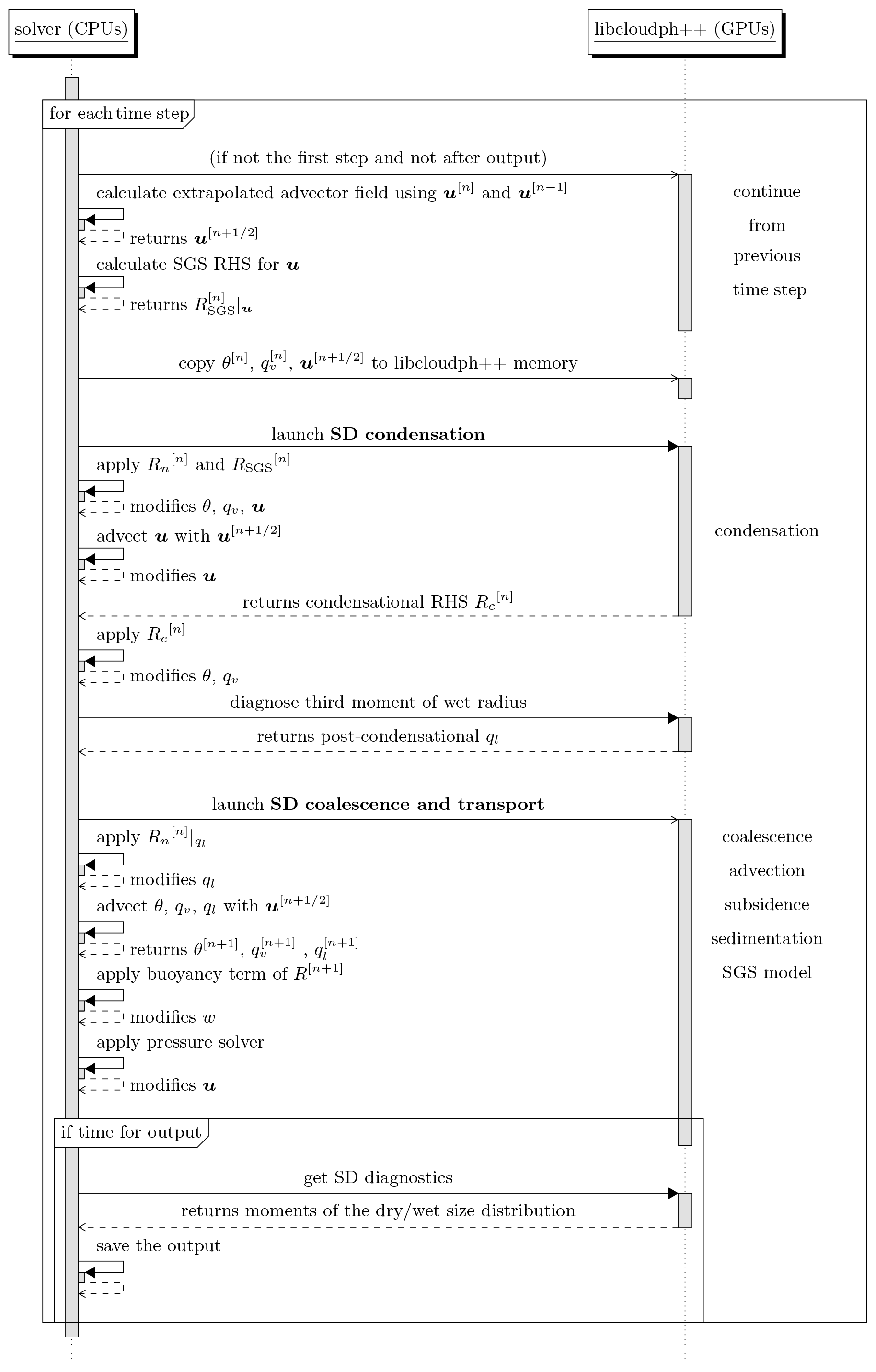
Figure 1 UML sequence diagram showing the order of operations in the UWLCM 2.0 model. Right-hand-side terms are divided into condensational, non-condensational and subgrid-scale parts; $R=R_{\mathrm{c}}+R_{\mathrm{n}}+R_{\mathrm{SGS}}$. Other notation follows Dziekan et al. (2019).

All CPU computations are done in double precision. Most of the GPU computations are done in single precision. The only exception is high-order polynomials, e.g., in the equation for the terminal velocity of droplets, which are done in double precision. So far, UWLCM has been used to model stratocumuli (Dziekan et al., 2019, 2021b), cumuli (Grabowski et al., 2019; Dziekan et al., 2021b) and rising thermals (Grabowski et al., 2018).

3 Adaptation to distributed memory systems

The strategy of adapting UWLCM to distributed memory systems was developed with a focus on UWLCM-SDM simulations with Lagrangian microphysics computed by GPUs. Therefore, this most complicated case is discussed first. Simpler cases with microphysics calculated by CPUs will be discussed afterwards.

The difficulty in designing a distributed memory implementation of code in which CPUs and GPUs simultaneously conduct different tasks is in obtaining a balanced workload distribution between different processing units. This is because GPUs have a higher throughput than CPUs, but device memory is rather low, which puts an upper limit on the GPU workload. Taking this into account, we chose to use a domain decomposition approach that is visualized in Fig. 2. The modeled domain is divided into equal slices along the horizontal x axis. Computations in each slice are done by a single MPI process, which can control multiple GPUs and CPU threads. Cloud microphysics within the slice are calculated on GPUs, with super-droplets residing in the device memory. Eulerian fields in the slice reside in the host memory and their evolution is calculated by CPU threads. Since the CPU and GPU data attributed to a process are colocated in the modeled space, all CPU-to-GPU and GPU-to-CPU communications happen via PCI-Express and do not require inter-node data transfer. The only inter-node communications are CPU-to-CPU and GPU-to-GPU. If an MPI process controls more than one GPU, computations within the subdomain of that process are divided among the GPUs also using domain decomposition along the x axis. Intra-node communication between GPUs controlled by a single process makes use of the NVIDIA GPUDirect Peer to Peer technology, which allows direct transfers between memories of different devices. Intra-node and inter-node transfers between GPUs controlled by different processes are handled by the MPI implementation. If the MPI implementation uses the NVIDIA GPUDirect Remote Direct Memory Access (RDMA) technology, inter-node GPU-to-GPU transfers go directly from the device memory to the interconnect, without host memory buffers.

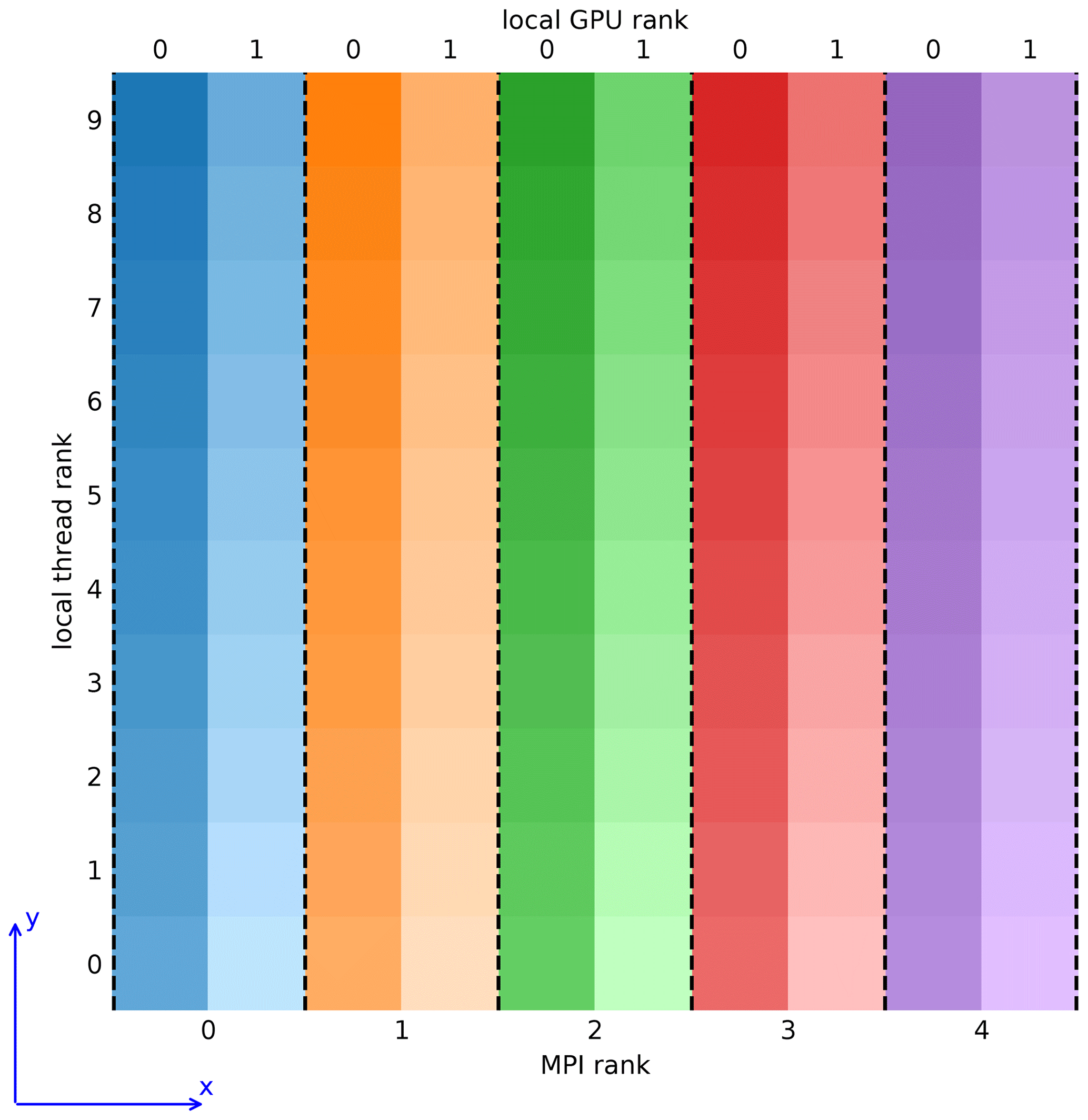
Figure 2 Visualization of the domain decomposition approach of UWLCM. Top–down view on a grid with 10 cells in each horizontal direction. Scalar variables are located at cell centers and vector variables are located at cell walls. Computations are divided among five MPI processes, each controlling 2 GPUs and 10 CPU threads. Local thread/GPU rank is the rank within the respective MPI process. Dashed lines represent boundaries over which communications need to be done using MPI assuming periodic horizontal boundary conditions.

Computations are divided between CPU threads of a process using domain decomposition of the process' subdomain but along the y axis. The maximum number of GPUs that can be used in a simulation is equal to the number of cells in the x direction. MPI communications are done using two communicators: one for the Eulerian data and one for the Lagrangian data. Transfers of the Eulerian data are handled simultaneously by two threads, one for each boundary that is perpendicular to the x axis. This requires that the MPI implementation supports the MPI_THREAD_MULTIPLE thread level. Transfers of the Lagrangian data are handled by the thread that controls the GPU that is on the edge of the process' subdomain. Collective MPI communication is done only on the Eulerian variables and most of it is associated with solving the pressure problem.

It is possible to run simulations with microphysics, either Lagrangian particle-based or bulk, computed by CPUs. In the case of bulk microphysics, microphysical properties are represented by Eulerian fields that are divided between processes and threads in the same manner as described in the previous paragraph, i.e., like the Eulerian fields in UWLCM-SDM. In UWLCM-SDM with microphysics computed by CPUs, all microphysical calculations in the subdomain belonging to a given MPI process are divided amongst the process' threads by the NVIDIA Thrust library (Bell and Hoberock, 2012).

File output is done in parallel by all MPI processes using the parallel HDF5 C++ library (, ).

4 Performance tests

4.1 Simulation setup

Model performance is tested in simulations of a rising moist thermal (Grabowski et al., 2018). In this setup, an initial spherical perturbation is introduced to a neutrally stable atmosphere. Within the perturbation, water vapor content is increased to obtain RH =100 %. With time, the perturbation is lifted by buoyancy and water vapor condenses within it. We chose this setup because it has significant differences in buoyancy and cloud formation already at the start of a simulation. This puts the pressure solver and microphysics model to test without the need of a spinup period.

Subgrid-scale diffusion of Eulerian fields is modeled with the Smagorinsky scheme. The SGS motion of hydrometeors is modeled with a scheme described in Grabowski and Abade (2017). Model time step length is 0.5 s. Substepping is done to achieve a time step of 0.1 s for condensation and coalescence. These are values typically used when modeling clouds with UWLCM. No output of model data is done.

4.2 Computers used

Performance tests were run on three systems: “Rysy”, “a02” and “Prometheus”. Hardware and software of these systems are given in Tables 1 and 2, respectively. Rysy and a02 were used only in the single-node tests, while Prometheus was used both in single- and multi-node tests. Prometheus has 72 GPU nodes connected with Infiniband. We chose to use the MVAPICH2 2.3.1 MPI implementation on Prometheus because it supports the MPI_THREAD_MULTIPLE thread level, is CUDA-aware and is free to use. Another implementation that meets these criteria is OpenMPI, but it was found to give greater simulation wall time in scaling tests of “libmpdata++” (Appendix B). The NVIDIA GPUDirect RDMA was not used by the MPI implementation because it is not supported by MVAPICH2 for the type of interconnect used on Prometheus. MVAPICH2 does not allow more than one GPU per process. Therefore multi-node tests were done for two processes per node, each process controlling 1 GPU and 12 CPU threads.

Table 1 List of hardware on the systems used. Computing performance and memory bandwidths are maximum values provided by the processing unit producer. Power usage of a processing unit is measured by the thermal design power (TDP).

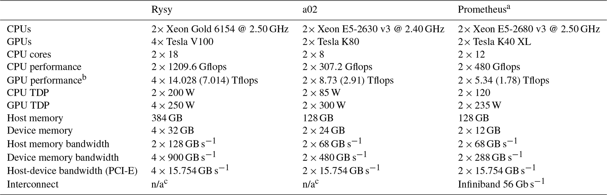
^a The cluster has 72 such nodes.
^b Single-precision performance. Double-precision performance is given in brackets. Almost all GPU computations are done in single precision.
^c Used in single-node tests only.

Table 2 List of software on the systems used.

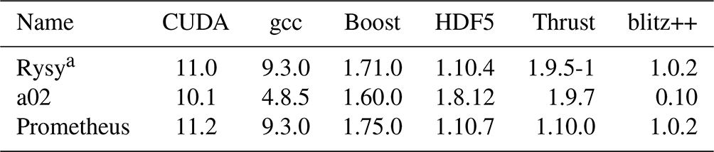
^a Software from a Singularity container distributed with UWLCM.

4.3 Performance metrics

The wall time taken to complete one model time step t_tot is divided into three parts: $t_{\mathrm{tot}}=t_{\mathrm{CPU}}+t_{\mathrm{GPU}}+t_{\mathrm{CPU}\mathrm{\&}\mathrm{GPU}}$, where

• t_CPU is the time when the CPU is performing work and the GPU is idle,

• t_GPU is the time when the GPU is performing work and the CPU is idle,

• t_CPU&GPU is the time when the CPU and the GPU are performing work simultaneously.

The total time of CPU (GPU) computations is $t_{\mathrm{CPU}}^{\mathrm{tot}}=t_{\mathrm{CPU}}+t_{\mathrm{CPU}\mathrm{\&}\mathrm{GPU}}$ ($t_{\mathrm{GPU}}^{\mathrm{tot}}=t_{\mathrm{GPU}}+t_{\mathrm{CPU}\mathrm{\&}\mathrm{GPU}}$). The degree to which CPU and GPU computations are parallelized is measured with $t_{\mathrm{CPU}\mathrm{\&}\mathrm{GPU}}/t_{\mathrm{tot}}$. The timings t_CPU, t_GPU and t_CPU&GPU are obtained using a built-in timing functionality of UWLCM that is enabled at compile time by setting the UWLCM_TIMING CMake variable. The timing functionality does not have any noticeable effect on simulation wall time. The timer for GPU computations is started by a CPU thread just before a task is submitted to the GPU and is stopped by a CPU thread when the GPU task returns. Therefore GPU timing in t_CPU&GPU and in t_GPU includes the time it takes to dispatch (and to return from) the GPU task.

4.4 Single-node performance

In this section we present tests of the computational performance of UWLCM-SDM run on a single-node system. The goal is to determine how the parallelization of CPU and GPU computations can be maximized. We also estimate the speedup achieved thanks to the use of GPUs. No MPI communications are done in these tests. The size of the Eulerian computational grid is $\mathrm{128}\times \mathrm{128}\times \mathrm{128}$ cells. In the super-droplet method, the quality of the microphysics solution depends on the number of super-droplets. We denote the initial number of super-droplets per cell by N_SD. We perform a test for different values of N_SD. The maximum possible value of N_SD depends on available device memory.

The average wall time it takes to do one model time step is plotted in Fig. 3. The time complexity of Eulerian computations depends on grid size and, ideally, does not depend on N_SD. In reality, we see that $t_{\mathrm{CPU}}^{\mathrm{tot}}$ slightly increases with N_SD. The space and time complexity of Lagrangian computations increases linearly with N_SD (Shima et al., 2009). It is seen that $t_{\mathrm{GPU}}^{\mathrm{tot}}$ in fact increases linearly with N_SD, except for low values of N_SD. For N_SD=3, CPU computations take longer than GPU computations ($t_{\mathrm{CPU}}^{\mathrm{tot}}>t_{\mathrm{GPU}}^{\mathrm{tot}}$) and almost all GPU computations are done in parallel with CPU computations (t_GPU≈0). As N_SD is increased, we observe that both t_tot and t_CPU&GPU increase, with t_CPU&GPU increasing faster than t_tot, and that t_CPU decreases. This trend continues up to some value of N_SD, for which $t_{\mathrm{CPU}}^{\mathrm{tot}}\approx t_{\mathrm{GPU}}^{\mathrm{tot}}$. Parallelization of CPU and GPU computations ($t_{\mathrm{CPU}\mathrm{\&}\mathrm{GPU}}/t_{\mathrm{tot}}$) is highest for this value of N_SD. If N_SD is increased above this value, GPU computations take longer than CPU computations, t_tot increases linearly and the parallelization of CPU and GPU computations decreases. The threshold value of N_SD depends on the system; it is 10 on Prometheus, 32 on a02 and 64 on Rysy. This difference comes from differences in relative CPU-to-GPU computational power between these systems. In LES, N_SD is usually between 30 and 100. The test shows that high parallelization of CPU and GPU computations, with $t_{\mathrm{CPU}\mathrm{\&}\mathrm{GPU}}/t_{\mathrm{tot}}$ up to 80 %, can be obtained in typical cloud simulations.

Figure 3 Single-node (no MPI) UWLCM-SDM performance for different hardware. The wall time per model time step averaged over 100 time steps. The results of LES of a rising thermal done on three different systems for a varying number of super-droplets, N_SD. t_CPU, t_GPU and t_CPU&GPU are wall times of CPU-only, GPU-only and parallel CPU and GPU computations, respectively. These timings are presented as stacked areas of different color. Total wall time per time step t_tot is the upper boundary of the green area. The dashed red line is the percentage of time spent on parallel CPU and GPU computations.

In UWLCM-SDM, microphysical computations can also be done by the CPU. From the user perspective, all that needs to be done is to specify “–backend=OpenMP” at runtime. To investigate how much speedup is achieved by employing GPU resources, in Fig. 4 we plot the time step wall time of CPU-only simulations (with microphysics computed by the CPU) and of CPU + GPU simulations (with microphysics computed by the GPU). The estimated energy cost per time step is also compared in Fig. 4. We find that simulations that use both CPUs and GPUs take between 10 to 130 times less time and use between 10 to 60 times less energy than simulations that use only CPUs. Speedup and energy savings increase with N_SD and depend on the number and type of CPUs and GPUs. It is important to note that microphysics computations in UWLCM-SDM are dispatched to CPU or GPU by the NVIDIA Thrust library. It is reasonable to expect that the library is better optimized for GPUs because it is developed by the producer of the GPU.

Figure 4 Wall time (a–c) and energy usage (d–f) per time step of CPU-only simulations (blue) and simulations utilizing both CPU and GPU (orange). In CPU-only simulations, energy usage is t_tot×P_CPU, where P_CPU is the sum of thermal design power of all CPUs. In CPU + GPU simulations, energy usage is $t_{\mathrm{CPU}}^{\mathrm{tot}}\times P_{\mathrm{CPU}}+t_{\mathrm{GPU}}^{\mathrm{tot}}\times P_{\mathrm{GPU}}$, where P_GPU is the sum of the thermal design power of all GPUs. P_CPU and P_GPU are listed in Table 1. Results are averaged over 100 time steps of UWLCM-SDM simulations on different single-node machines.

4.5 Multi-node performance

Computational performance of UWLCM-SDM, UWLCM-B1M and UWLCM-B2M on distributed memory systems is discussed in this section. We consider four scenarios in which UWLCM is run on a distributed memory system for different reasons. Depending on the scenario and on the number of nodes used, the number of Eulerian grid cells is between 0.5 and 18.5 million, and number of Lagrangian particles is between 40 million and 18.5 billion. Details of the simulation setup for each scenario are given in Table 3. The scenarios are

• “strong scaling”. More nodes are used in order to decrease the time it takes to complete the simulation.

• “SD scaling”. More nodes are used to increase the total device memory, allowing for more SD to be modeled, while the grid size remains the same. This results in weak scaling of the GPU workload and strong scaling of the CPU workload. This test is applicable only to UWLCM-SDM.

• “2D grid scaling”. As more nodes are used, the number of grid cells in the horizontal directions is increased, while the number of cells in the vertical is constant. In UWLCM-SDM, the number of SDs per cell is constant. Therefore, as more cells are added, the total number of SDs in the domain increases. This results in weak scaling of both CPU and GPU workloads. This test represents two use cases: domain size increase and horizontal-resolution refinement. Typically in cloud modeling, domain size is increased only in the horizontal because clouds form only up to a certain altitude.

• “3D grid scaling”. Similar to 2D grid scaling, but more cells are used in each dimension. This would typically be used to increase the resolution of a simulation.

In each case, the maximum number of super-droplets that fits the device memory is used in UWLCM-SDM. The only exception is the strong scaling test in which, as more nodes are added, the number of SD per GPU decreases. Note how SD scaling is similar to strong scaling, but with more SDs added as more GPUs are added. Also note that the 2D grid scaling and 3D grid scaling tests are similar, but with differences in the sizes of distributed memory data transfers.

Table 3 Details of multi-node scaling tests. n_x, n_y and n_z is the total number of Eulerian grid cells in the respective direction. N_SD is the initial number of super-droplets per Eulerian grid cell. N_nodes is the number of nodes used for the simulation. Number of Eulerian grid cells in the domain is equal to $n_x\times n_y\times n_z$. Number of super-droplets in the domain is equal to $n_x\times n_y\times n_z\times N_{\mathrm{SD}}$. Workload per CPU is estimated assuming that it is proportional to the number of grid cells per CPU only. Workload per GPU is estimated assuming that it is proportional to the number of super-droplets per GPU only. MPI transfers, data transfers between host and device memories, and GPU handling of information about Eulerian cells are not included in these workload estimates. Data transfer sizes are for copies between different MPI processes but do not include copies between host and device memories of the same process. Data transfer sizes are estimated assuming that time step length and air flow velocities do not change with grid size. t¹ is the wall time on a single node. $t_{\mathrm{GPU}}^{\mathrm{2}}$ is the wall time of GPU and CPU + GPU calculations in a simulation on two nodes.

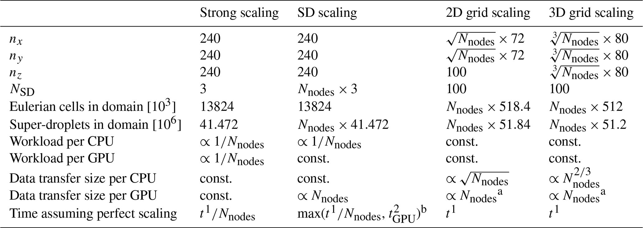
^a Assuming that grid scaling is used to refine the resolution, as done in this paper. If it is done to increase the domain, the data transfer size per GPU scales in the same way as the one per CPU.
^b GPU time from two-node simulation is taken as reference because it is ca. 15 % lower than on a single node. A plausible explanation for this is that, although the number of SDs per GPU does not depend on the number of nodes, GPUs also store information about conditions in grid cells, and the number of grid cells per GPU decreases as more nodes are used. For more than two nodes, GPU calculation time is approximately the same as for two nodes.

UWLCM-SDM simulation time versus the number of nodes used is plotted in Fig. 5. First, we discuss the strong scaling scenario. We find that most of the time is spent on CPU-only computations. This is because in this scenario N_SD=3, below the threshold value of N_SD=10 determined by the single-node test (Sect. 4.4). As more nodes are added, t_CPU&GPU and t_tot decrease. The ratio of these two values, which describes the amount of parallelization of CPU and GPU computations, is low (30 %) in a single-node run and further decreases, however slowly, as more nodes are used.

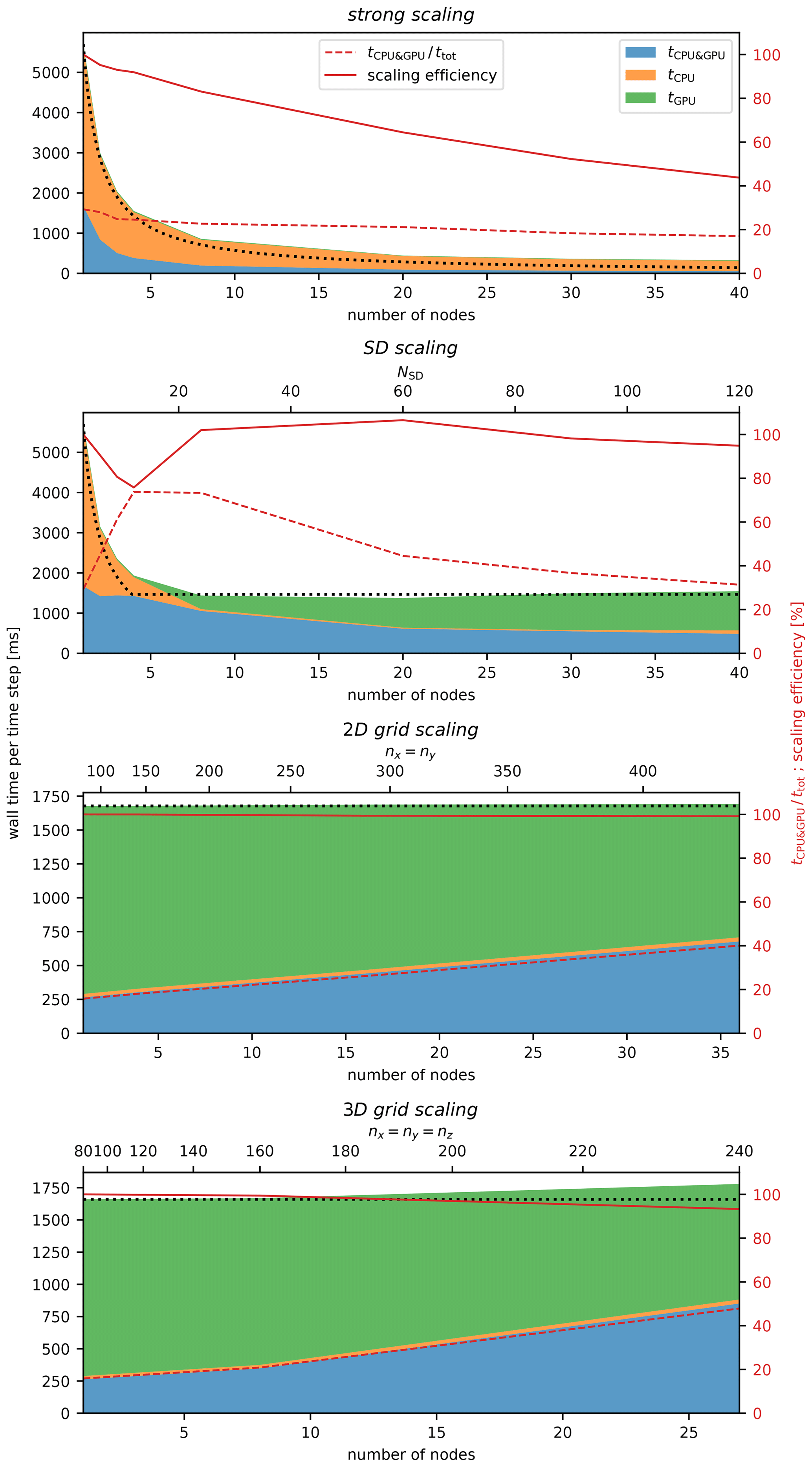
Figure 5 As in Fig. 3 but for multi-node tests done on the Prometheus cluster for different scaling scenarios. The dotted black line is perfect scaling of t_tot. The solid red line is scaling efficiency, defined as t_tot assuming perfect scaling divided by the actual t_tot. Perfect scaling is defined in Table 3.

Better parallelization of CPU and GPU computations is seen in the SD scaling scenario. In this scenario, the CPU workload scales the same as in the strong scaling scenario, but the workload per GPU remains constant. The largest value of $t_{\mathrm{CPU}\mathrm{\&}\mathrm{GPU}}/t_{\mathrm{tot}}$, approximately 80 %, is found for N_SD=10. The same value of N_SD was found to give the highest $t_{\mathrm{CPU}\mathrm{\&}\mathrm{GPU}}/t_{\mathrm{tot}}$ in the single-node tests (Sect. 4.4). We observe that $t_{\mathrm{GPU}}^{\mathrm{tot}}$ is approximately constant. Given the weak scaling of the GPU workload in this scenario, we conclude that the cost of GPU-GPU MPI communications is small. The small cost of GPU-GPU MPI communications, together with the fact that for N_SD>10 the total time of computations is dominated by GPU computations, gives very high scaling efficiencies of around 100 %.

Among the scenarios, 2D and 3D grid scaling are weak scaling tests which differ in the way the size of CPU MPI communications scales. We find that wall time per time step t_tot scales very well (scaling efficiency exceeds 95 %) and that t_tot is dominated by $t_{\mathrm{GPU}}^{\mathrm{tot}}$ ($t_{\mathrm{GPU}}^{\mathrm{tot}}>t_{\mathrm{CPU}}^{\mathrm{tot}}$). The latter observation is consistent with the fact that the number of super-droplets (N_SD=100) is larger than the threshold, N_SD=10, determined in single-node tests. As in SD scaling, approximately constant $t_{\mathrm{GPU}}^{\mathrm{tot}}$ indicates the low cost of MPI communications between GPUs. Contrary to $t_{\mathrm{GPU}}^{\mathrm{tot}}$, $t_{\mathrm{CPU}}^{\mathrm{tot}}$ clearly increases with the number of nodes. This shows that the cost of CPU–CPU MPI communications is non-negligible. The increase in $t_{\mathrm{CPU}}^{\mathrm{tot}}$ does not cause an increase in t_tot because additional CPU computations are done simultaneously with GPU computations and $t_{\mathrm{GPU}}^{\mathrm{tot}}>t_{\mathrm{CPU}}^{\mathrm{tot}}$ in the studied range of the number of nodes. It is reasonable to expect that $t_{\mathrm{GPU}}^{\mathrm{tot}}$ scales better than $t_{\mathrm{CPU}}^{\mathrm{tot}}$ also for more nodes than used in this study. In that case, there should be some optimal number of nodes for which $t_{\mathrm{GPU}}^{\mathrm{tot}}\approx t_{\mathrm{CPU}}^{\mathrm{tot}}$. For this optimal number of nodes both scaling efficiency and parallelization of CPU and GPU computations are expected to be high.

Comparison of scaling of t_tot in UWLCM-B1M, UWLCM-B2M and UWLCM-SDM is shown in Fig. 6. UWLCM-B1M and UWLCM-B2M use simple microphysics schemes that are computed by the CPU. UWLCM-B2M, which has four Eulerian prognostic variables for microphysics, is more complex than UWLCM-B1M, which has two. Regardless of this, wall time is very similar for UWLCM-B1M and UWLCM-B2M. Wall time of UWLCM-SDM, which uses a much more complex microphysics scheme, is higher by a factor that depends on the number of SD. In 2D grid scaling and 3D grid scaling tests of UWLCM-SDM there are 100 SDs per cell, which is a typical value used in LES. Then, on a single node, UWLCM-SDM simulations take approximately 8 times longer than UWLCM-B1M or UWLCM-B2M simulations. However, UWLCM-SDM scales better than UWLCM-B1M and UWLCM-B2M because scaling cost is associated with the Eulerian part of the model and in UWLCM-SDM this cost does not affect total wall time, as total wall time is dominated by Lagrangian computations. As a result, the difference in wall time between UWLCM-SDM and UWLCM-B1M or UWLCM-B2M decreases with the number of nodes. For the largest number of nodes used in 2D grid scaling and 3D grid scaling, UWLCM-SDM simulations take approximately 5 times longer than UWLCM-B1M or UWLCM-B2M simulations. The strong scaling UWLCM-SDM test uses three SDs per cell. For such a low number of SDs, time complexity of Lagrangian computations in UWLCM-SDM is low and we see that the wall time and its scaling are very similar to that of UWLCM-B1M and UWLCM-B2M.

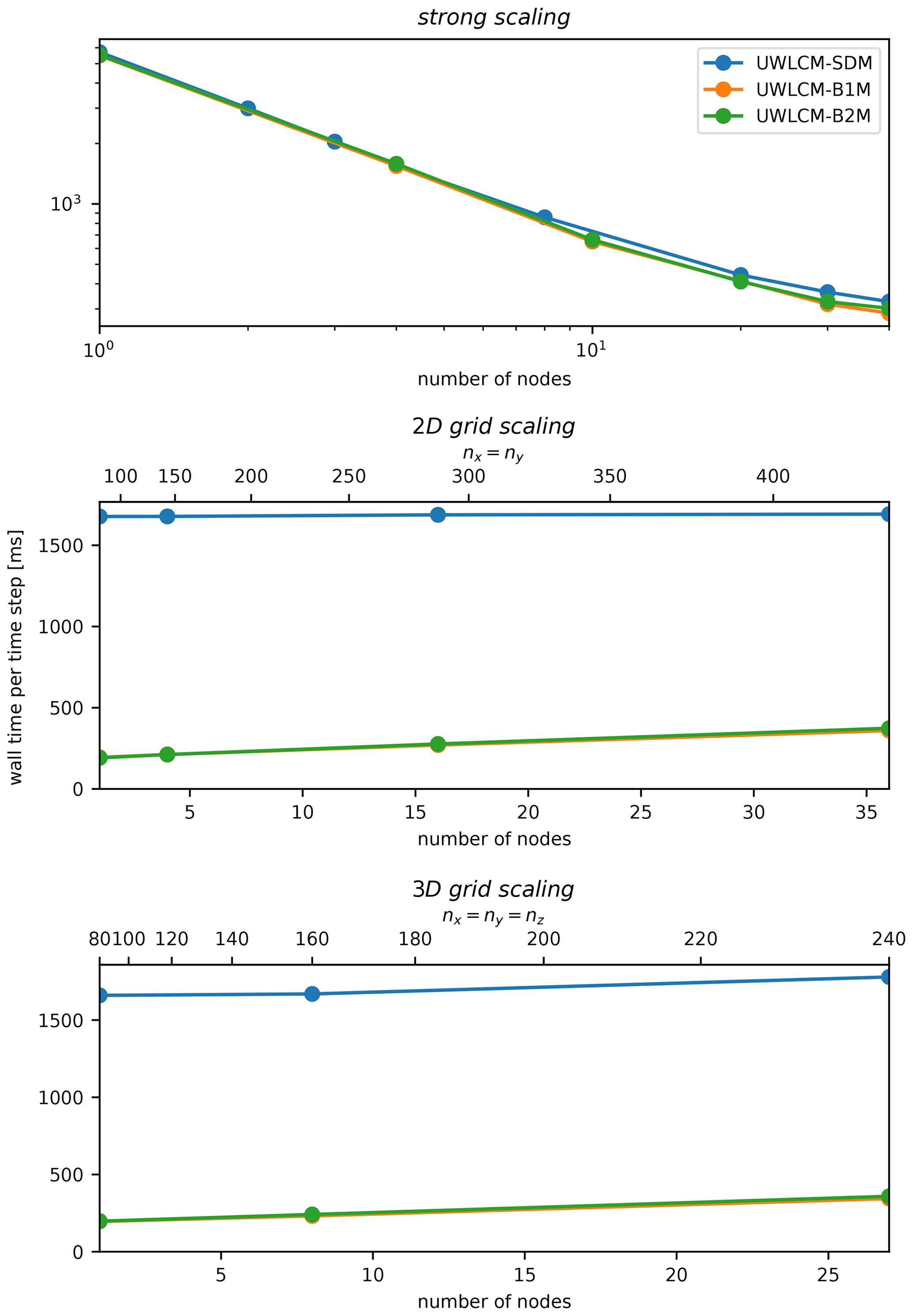
Figure 6 Multi-node model performance for different microphysics schemes. Wall time per model time step averaged over 100 time steps. Results of LES of a rising thermal done on the Prometheus cluster for different scaling scenarios.

5 Summary

A numerical model with Lagrangian particles embedded in an Eulerian fluid flow has been adapted to clusters equipped with GPU accelerators. On multi-node systems, computations are distributed among processes using static domain decomposition. The Eulerian and Lagrangian computations are done in parallel on CPUs and GPUs, respectively. We identified simulation parameters for which the amount of time during which CPUs and GPUs work in parallel is maximized.

Single-node performance tests were done on three different systems, each equipped with multiple GPUs. The percentage of time during which CPUs and GPUs compute simultaneously depends on the ratio of CPU to GPU workloads. GPU workload depends on the number of Lagrangian computational particles. For an optimal workload ratio, parallel CPU and GPU computations can take more than 80 % of wall time. This optimal workload ratio depends on the relative computational power of CPUs and GPUs. On all systems tested, the workload ratio was optimal for between 10 and 64 Lagrangian particles per Eulerian cell. If only CPUs are used for computations, simulations take up to 120 times longer and consume up to 60 times more energy than simulations that use both CPUs and GPUs. We conclude that GPU accelerators enable the running of useful scientific simulation on single-node systems at a decreased energy cost.

Computational performance of the model on a distributed memory system was tested on the Prometheus cluster. We found that the cost of communication between nodes slows down computations related to the Eulerian part of the model by a much higher factor than computations related to the Lagrangian part of the model. For example, in a weak scaling scenario (3D grid scaling) $t_{\mathrm{CPU}}^{\mathrm{tot}}$ is approximately 3 times larger on 27 nodes than on one node, while $t_{\mathrm{GPU}}^{\mathrm{tot}}$ is increased by only around 7 % (Fig. 5). The reason why Eulerian computations scale worse than Lagrangian computation is that solving the pressure perturbation, which is done by the Eulerian component, requires collective communications, while the Lagrangian component requires peer-to-peer communications only. In single-node simulations on Prometheus an optimal ratio of CPU to GPU workloads is seen for 10 Lagrangian particles per Eulerian cell. In the literature, the number of Lagrangian particles per Eulerian cell is typically higher: between 30 and 100 (Shima et al., 2009; Dziekan et al., 2019, 2021b). When such a higher number of Lagrangian particles is used in single-node simulations on Prometheus, most of the time is spent on Lagrangian computations. However, in multi-node runs, Eulerian computation time scales worse than Lagrangian computation time. Since Eulerian and Lagrangian computations are done simultaneously, there is an optimal number of nodes for which the amount of time during which CPUs and GPUs work in parallel is maximized and the scaling efficiency is high. In scenarios in which GPU computations take most of the time, scaling efficiency exceeds 95 % for up to 40 nodes. The fraction of time during which CPUs and GPUs work in parallel is between 20 % and 50 % for the largest number of nodes used. In weak scaling scenarios, the fraction of time during which both processing units work could be increased by using more nodes, but it was not possible due to the limited size of the cluster. Single-node simulations with Lagrangian microphysics computed by GPUs are around 8 times slower than simulations with bulk microphysics computed by CPUs. However, the difference decreases with the number of nodes. For 36 nodes, simulations with Lagrangian microphysics are 5 times slower, and the difference should be further reduced if more nodes were used.

Our approach of using CPUs for Eulerian calculations and GPUs for Lagrangian calculations results in CPUs and GPUs computing simultaneously for a majority of the time step and gives good scaling on multi-node systems with several dozens of nodes. The same approach can be used in other numerical models with Lagrangian particles embedded in an Eulerian flow.

Appendix A: Software

UWLCM is written in C++14. It makes extensive use of two C++ libraries that are also developed at the Faculty of Physics of the University of Warsaw: libmpdata++ (Jaruga et al., 2015; Waruszewski et al., 2018) and libcloudph++ (Arabas et al., 2015; Jaruga and Pawlowska, 2018). Libmpdata++ is a collection of solvers for generalized transport equations that use the multidimensional positive definite advection transport algorithm (MPDATA) algorithm. Libcloudph++ is a collection of cloud microphysics schemes.

In libcloudph++, the particle-based microphysics algorithm is implemented using the NVIDIA Thrust library. Thanks to that, the code can be run on GPUs as well as on CPUs. It is possible to use multiple GPUs on a single machine, without MPI. Then, each GPU is controlled by a separate thread and communications between GPUs are done with the asynchronous “cudaMemcpy”. Libmpdata++ uses multidimensional array containers from the blitz++ library (Veldhuizen, 1995). Threading can be done either with OpenMP, Boost.Thread or std::thread. In UWLCM we use the OpenMP threading as it was found to be the most efficient. Output in UWLCM is done using the HDF5 output interface that is part of libmpdata++. It is based on the thread-safe version of the C++ HDF5 library. UWLCM, libcloudph++ and libmpdata++ make use of various components of the Boost C++ library (Boost C++ Libraries, 2022). In order to have parallel CPU and GPU computations in UWLCM, functions from libmpdata++ and from libcloudph++ are launched using std::async. UWLCM, libcloudph++ and libmpdata++ are open-source software distributed via the Github repository https://github.com/igfuw/ (last access: 14 April 2022). They have test suits that are automatically run on Github Actions. To facilitate deployment, a Singularity container with all necessary dependencies is included in UWLCM (https://cloud.sylabs.io/library/pdziekan/default/uwlcm) (last access: 14 April 2022).

Libcloudph++ and libmpdata++ have been adapted to work on distributed memory systems. This has been implemented using the C interface of MPI in libcloudph++ and the Boost.MPI library in libmpdata++. Tests of the scalability of libmpdata++ are presented in Appendix B.

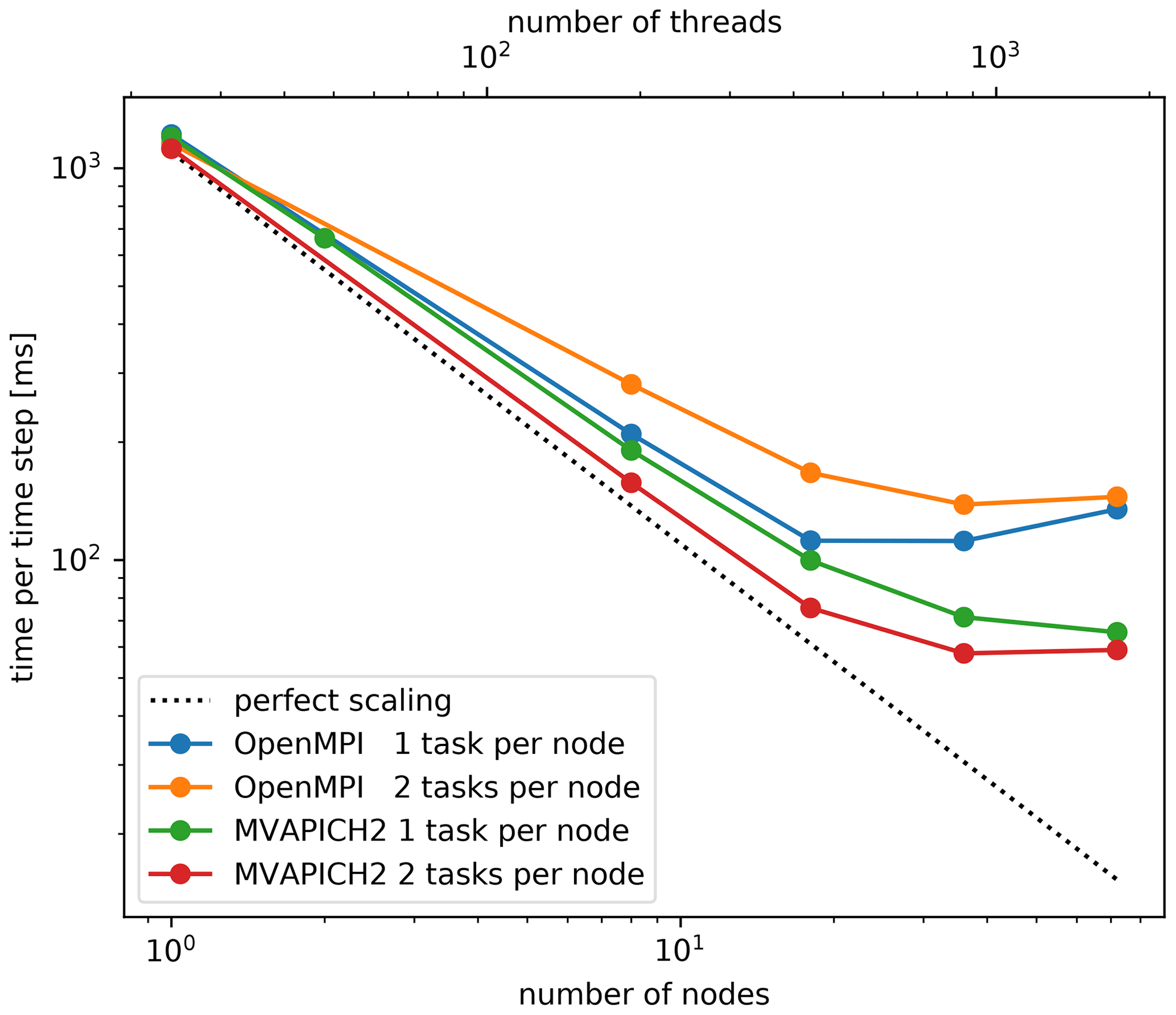
Figure A1 Strong scaling test of the libmpdata++ library. Wall time per time step of a dry planetary boundary layer simulation. The dotted black line shows perfect scaling.

Appendix B: Scalability of libmpdata++

UWLCM uses the libmpdata++ library for solving the equations that govern the time evolution of Eulerian variables. The library had to be adapted for work on distributed memory systems. The domain decomposition strategy is as in Fig. 2 but without GPUs. Here, we present strong scaling tests of standalone libmpdata++. The tests are done using a dry planetary boundary layer setup, which is a part of the libmpdata++ test suite. The grid size is $\mathrm{432}\times \mathrm{432}\times \mathrm{51}$. Tests were done on the Prometheus cluster. Note that all libmpdata++ calculations are done on CPUs. Two implementations of MPI are tested: OpenMPI v4.1.0 and MVAPICH2 v2.3.1. Note that Prometheus has two GPUs per node, but MVAPICH2 does not support more than one GPU per process, so two processes per node would need to be run in UWLCM-SDM. OpenMPI does not have this limitation. For this reason in the libmpdata++ scalability tests we consider two scenarios: one with two processes per node and the other with one process per node. In the case with two processes per node, each process controls half of the available threads. Test results are shown in Fig. A1. In general, better performance is seen with MVAPICH2 than with OpenMPI. Running two processes per node improves performance in MVAPICH2 but decreases performance in OpenMPI. In the best case, scaling efficiency exceeds 80 % for up to 500 threads.