the Creative Commons Attribution 4.0 License.
the Creative Commons Attribution 4.0 License.
 | 10 Jun 2022
Transient climate simulations of the Holocene (version 1) – experimental design and boundary conditions
Dabang Jiang
Ran Zhang
Baohuang Su
The Holocene, which started approximately 11.5 ka, is the latest interglacial period with several rapid climate changes with timescales, from decades to centuries, superimposed on the millennium-scale mean climate trend. Climate models provide useful tools to investigate the underlying dynamic mechanisms for the climate change during this well-studied time period. Thanks to the improvements in the climate model and computational power, transient simulation of the Holocene offers an opportunity to investigate the climate evolution in response to time-varying external forcings and feedbacks. Here, we present the design of a new set of transient experiments for the whole Holocene from 11.5 ka to the preindustrial period (1850; HT-11.5 ka) to investigate both the combined and separated effects of the main external forcing of orbital insolation, atmospheric greenhouse gas (GHG) concentrations, and ice sheets on the climate evolution over the Holocene. The HT-11.5 ka simulations are performed with a relatively high-resolution version of the comprehensive Earth system model CESM1.2.1 without acceleration, both fully and singly forced by time-varying boundary conditions of orbital configurations, atmospheric GHGs, and ice sheets. Preliminary simulation results show a slight decrease in the global annual mean surface air temperature from 11.5 to 7.5 ka due to both changes in orbital insolation and GHG concentrations, with an abrupt cooling at approximately 7.5 ka, which is followed by a continuous warming until the preindustrial period, mainly due to increased GHG concentrations. Both at global and zonal mean scales, the simulated annual and seasonal temperature changes at 6 ka lie within the range of the 14 PMIP4 model results and are overall stronger than their arithmetic mean results for the Middle Holocene simulations. Further analyses on the HT-11.5 ka transient simulation results will be covered by follow-up studies.
- Article
(3891 KB) - Full-text XML
- BibTeX
- EndNote


1.1 Climate evolution over the Holocene
Since the end of the Younger Dryas cooling event at ∼11.5 ka, the global climate has entered the Holocene period. The Holocene is the latest interglacial period in the Quaternary glacial–interglacial cycles, which has experienced strong global environmental changes mainly due to the retreat of continental ice sheets, changes in atmospheric greenhouse gas (GHG) concentrations, and variations in the seasonal insolation associated with changes in the Earth's orbital parameters and solar variability (Mayewski et al., 2004). Although previous attempts to subdivide the Holocene still remain inconclusive, the Holocene can roughly be divided into the following three periods (Nesje and Dahl, 1993): the Early Holocene, with a high boreal summer insolation and a large remnant ice sheet in North America, the Holocene Hypsithermal, with a continuing high boreal summer insolation but a small remnant North American ice sheet, and the Late Holocene Neoglacial, with a declining boreal summer insolation (Wanner and Ritz, 2011; Wanner et al., 2011; Walker et al., 2012).
The Early Holocene, approximately spanning from 11.5 to 9 ka, represents the last transition from full glacial to interglacial conditions, which is characterized by a warming trend, mainly in the northern mid- and high-latitudes, as revealed from numerous reconstructions (e.g., Koerner and Fisher, 1990; Yuan et al., 2004; Wang et al., 2005; Hald et al., 2007; Vinther et al., 2008; Brooks et al., 2012; Shakun et al., 2012; Birks, 2015). In tropical regions, the change in precipitation was more prominent during the Early Holocene, among which the African Humid Period is one typical example (Gasse, 2001; Hoelzmann et al., 2004), in addition to a humidity climate in the Arabian Sea, the Bay of Bengal (Gupta et al., 2003; Staubwasser, 2006), and northern South America (Haug et al., 2001), which was suggested to be fundamentally affected by precession (e.g., Renssen et al., 2004). However, a drier climate was inferred from multi-evidence in central and southern South America (Maslin and Burns, 2000; Seltzer et al., 2000; Núñez et al., 2002) and westerlies-dominated North Asia, whereas monsoon-influenced East Asia was substantially wetter but with an asynchronous peak of precipitation in northeastern, northwestern, and northern China (An et al., 2000; Chen et al., 2008, 2019; Zhang et al., 2011).
The Holocene Hypsithermal, covering from about 9 to 5–6 ka, generally refers to the interval of warmth associated with the peak Holocene temperature, which is also called the Holocene Thermal Maximum, the Holocene Climatic Optimum, Altithermal, or Megathermal (Deevey and Flint, 1957; Wanner et al., 2008; Ljungqvist, 2011). The timing and spatial pattern of this period in different regions have long attracted the attention of researchers. Relative to the preindustrial period, the reconstructed Holocene maximum temperature appeared during 10–8 ka in the North Atlantic and the adjacent polar regions, which occurred during 7–5 ka in northern Europe and northwestern North America, and registered between Early and Middle Holocene at the northern mid- and high-latitudes, e.g., during 8.5–3.0 ka in China (Shi et al., 1993), and appeared to be time-transgressive across the western hemisphere of the Arctic (Kaufman et al., 2004), suggesting that these local warm periods were very likely not globally synchronous (Jansen et al., 2007). Different from the Northern Hemisphere, the southern mid- and high-latitudes experienced a drop in temperature during the Middle and Late Holocene, following the Early Holocene warming period (Shevenell et al., 2011). Concerning the moisture conditions, paleoenvironmental data consistently showed that the mid-continental extra-tropics were wetter, with cooler summers than today, during the Middle Holocene (Harrison et al., 2015).
The Late Holocene Neoglacial or Neoglaciation, lasting from about 5–6 ka to the preindustrial period, features an obvious increase in the number of glacial advances worldwide, mainly due to decreasing solar forcing in the boreal summer (Solomina et al., 2015). The global mean surface temperature during this period displayed a consistent cooling trend, as indicated from multi-proxy-based reconstructions (Wanner et al., 2008; Ljungqvist, 2011; Marcott et al., 2013; Kaufman et al., 2020a, 2020b; Zhang et al., 2022), which was suggested to be mainly due to the influence of orbital forcing together with the melting ice sheet in North America. In contrast, the Late Holocene warming trend was also supported by simulations (e.g., Liu et al., 2014, 2018) and by several reconstructions from subfossil pollen (Marsicek et al., 2018) and stalagmite records during the winter season (Baker et al., 2017), which was mainly attributed to rising atmospheric greenhouse gases (GHGs) and winter insolation. Therefore, it still remains inconclusive as to whether the Late Holocene was cooler or warmer. To reconcile this so-called Holocene temperature conundrum, further efforts should be taken to improve, both in simulations, by including solar irradiance forcing, land use changes, dust effects, and stratospheric chemistry and dynamics, and in reconstructions with higher spatial and temporal resolutions, a balanced distribution between marine and terrestrial and between the Northern Hemisphere and Southern Hemisphere data, and the representing proxies from both summer and winter seasons (Bova et al., 2021; Wanner, 2021; Zhang et al., 2022), as well as in the model–data assimilation approaches (Osman et al., 2021).
Superimposed on the millennium-scale mean climate trend during the above Holocene periods are several rapid cooling events on the timescales from decades to centuries (Wanner et al., 2011; Walker et al., 2012). Most of those events are characterized by cooling at northern mid- and high-latitudes, aridity at low-latitude monsoon regions, and major atmospheric circulation changes (Mayewski et al., 2004), which were generally inferred to relate to the freshwater outbreak caused by ice melting in the North Atlantic before 8.2 ka, the solar variability superimposed on long-term changes in insolation during the Middle and Late Holocene, and explosive volcanic eruptions and fluctuations in the thermohaline circulation (Mayewski et al., 2004; Magny et al., 2007; Wanner et al., 2011).
1.2 Transient modeling of the Holocene
Transient modeling of the Holocene offers an opportunity to examine the climate evolution in response to time-varying external forcings and feedbacks. Combined with proxy data, it is the most useful tool to comprehensively understand the causes for past complex and interrelating climate processes. Since the 1990s, the Paleoclimate Modeling Intercomparison Project (PMIP) has served to coordinate paleoclimate simulations and model–data comparisons (Joussaume and Taylor, 1995; Braconnot et al., 2007; Taylor et al., 2012), and it now enters its fourth phase (PMIP4; Kageyama et al., 2018), contributing to the current sixth phase of the Coupled Model Intercomparison Project (CMIP6; Eyring et al., 2016) and the Intergovernmental Panel on Climate Change (IPCC) Sixth Assessment Report (IPCC, 2022). The major focuses in PMIP4 include not only equilibrium (or time slice) simulations to investigate the impact of changes mainly in orbital forcing, e.g., during the Middle Holocene (6 ka), but also transient simulations of the last deglaciation from 21 to 9 ka with time-varying orbital forcing, GHGs, ice sheets, and other geographical changes (Ivanovic et al., 2016) and of the Holocene from 6 to 0 ka with temporal changes in orbital forcing and GHGs (Otto-Bliesner et al., 2017).
Up to now, a dozen transient simulations covering the Holocene have been carried out using global climate models with different complexities. For example, FOAM, a fully coupled global atmosphere–ocean general circulation model with a low resolution of (latitude × longitude), was used to run a transient simulation for the past 280 ka to examine the evolutionary response of global monsoons to orbital forcing, which is accelerated by a factor of 100 (Kutzbach et al., 2008). FAMOUS (Smith et al., 2008), a low-resolution () version of the HadCM3 (Gordon et al., 2000) coupled model, was used to conduct a number of accelerated transient experiments (by a factor of 10) for the last 120 ka to investigate the climate of the last glacial cycle (Smith and Gregory, 2012). A set of transient simulations of the last deglaciation for the past 26 ka was performed with a low-resolution () Earth system model MPI-ESM1.2 to explore differences in climate response to different underlying ice sheet reconstructions and methods of meltwater distribution (Kapsch et al., 2020), as suggested within the PMIP4 deglaciation protocol (Ivanovic et al., 2016). The Transient Climate Evolution of the past 21 ka (TraCE-21 ka; He, 2011), run with the low-resolution () National Center for Atmospheric Research (NCAR) Community Climate System Model (CCSM) version 3 (CCSM3), is widely used for examining the climate evolution since the last glacial maximum at global and regional scales (e.g., Liu et al., 2014, 2021; Wu et al., 2021). A fully coupled atmosphere–ocean–sea ice model ECBilt-CLIO, with a horizontal resolution of , was also used for transient simulations of the last deglaciation (last 21 ka) to investigate the effect of using accelerated (by a factor of 10) boundary conditions and of uncertainties in the initial state (Timm and Timmermann, 2007). Additionally coupled with a vegetation model, ECBilt-CLIO-VECODE3 was performed to investigate the global characterization of the Holocene thermal maximum for the last 9 ka (Renssen et al., 2012). A later-developed version, LOVECLIM, additionally coupled with carbon cycle and terrestrial ice sheets (Goosse et al., 2010), was employed to examine the Early Holocene (11.5–7 ka) warming (Zhang et al., 2016), the Holocene northern temperature and hydroclimate trends (Zhang et al., 2018, 2020), and the obliquity and CO2 effects on southern climate during the past 408 ka with an acceleration factor of 5 (Timmermann et al., 2014).
Concentrating more on the Holocene, transient simulations for the past 12 ka, run with an acceleration factor of 10 with the low-resolution () Community Earth System Model (CESM) version 1.0.3 (CESM1.0.3), showed a cooling trend during 5–0.15 ka by considering the volcanic forcing (Wan et al., 2020) and an increasing trend in the northern mid-latitude precipitation during 7–0 ka in response to the orbital forcing (Sun et al., 2020). A transient simulation of the last 8 ka, performed with the high-resolution () MPI-ESM1.2, additionally forced by solar variability and volcanic forcing, further revealed that both global warming and cooling modes coexisted during the Holocene (Bader et al., 2020), which also captured the global vegetation transitions and the time-transgressive end of the African Humid Period, as revealed in proxy data (Dallmeyer et al., 2020, 2021). Using a low-resolution () atmosphere–ocean–sea ice coupled model, KCM, with an acceleration factor of 10, a transient climate simulation of the past 9.5 ka was conducted to examine the summer precipitation across the Asian monsoon region in response to the orbital forcing (Jin et al., 2014). Besides, two versions of the IPSL model were used to run the transient simulations of the last 6 ka, indicating larger impacts of different model versions and experimental setups on the mean state of climate than on the associated interannual-to-decadal variability (Braconnot et al., 2019a, b; Crétat et al., 2020). In addition, the four Holocene transient simulations run with MPI-ESM1.2, two versions of the IPSL model, and AWI-ESM2 (Sidorenko et al., 2019) were compared to support the orbital forcing of the El Niño–Southern Oscillation (ENSO) amplitude since the Middle Holocene (Carré et al., 2021) and indicate the importance of the application of calendar transformation in the analysis of climate simulations when we perform multimodel comparisons (Shi et al., 2022).
1.3 A new set of Holocene transient experiments
Taken together, among the abovementioned Holocene transient simulations, only seven of them covered the whole Holocene of the past 11.5 ka, i.e., simulations with LOVECLIM for the past 408 ka, FOAM for the past 284 ka, FAMOUS for the past 120 ka, MPI-ESM1.2 for the past 26 ka, CCSM3 and ECBilt-CLIO for the past 21 ka, and CESM1.0.3 for the past 12 ka. They were performed with climate system models or Earth system models with intermediate complexity, all of which have relatively low spatial resolutions varying from to and/or use acceleration techniques with a factor from 5 to 100 to reduce computational resources. Note that, on the one hand, the model resolution determines the level of detail in its representation of the physical processes related to the topography, heat transport, sea ice cover, etc., which may have large effects on the Holocene climate evolution (Zhang et al., 2018). On the other hand, acceleration in transient simulations can also have a significant impact on the local climate history, for example, which will lead to damped and delayed temperature response to the boundary conditions in the North Atlantic (Timm and Timmermann, 2007). In addition, most models used for the Holocene transient simulations are fully forced by time-varying boundary conditions of orbital configurations, GHGs, and ice sheets, some of which are additionally forced by meltwater flux, land use/land cover, solar variability, or volcanic forcing, making it difficult to isolate their relative contribution to the past climate evolution.
In this context, it is urgent to carry out a new set of unaccelerated transient experiments focusing on the whole Holocene, since 11.5 ka, using the comprehensive Earth system model with relatively high spatial resolutions, considering both the full-forcing and single-forcing effects of several of the most important boundary conditions, including the orbital parameters, GHG concentrations, and ice sheets, on the Holocene climate evolution. This set of Holocene transient simulations for the last 11.5 ka will also fill in the gap between the PMIP4 transient Core experiments for the last deglaciation from 21 to 9 ka (Ivanovic et al., 2016) and the PMIP4 Tier 3 transient simulations for the Holocene from 6 to 0 ka (Otto-Bliesner et al., 2017).
The aim of this paper is to outline the model description (in Sect. 2), experimental setup, and boundary conditions (in Sect. 3) for the new Holocene transient climate experiments of the last 11.5 ka (henceforth HT-11.5 ka for brevity), with some preliminary results being provided in Sect. 4. Further analyses on these simulation results will be covered by follow-up studies.
The model used to run the HT-11.5 ka simulation in this study is the NCAR CESM version 1.2.1 (CESM1.2.1), which was released on December 2013 and was a relatively new version when we started this simulation in 2016. CESM is a fully coupled global Earth system model that provides state-of-the-art simulations of the Earth's past, present, and future climate states, with an earlier version 1 (CESM1) participating in the CMIP phase 5 (CMIP5; Taylor et al., 2012) and the later version 2 (CESM2) participating in the CMIP6 (Eyring et al., 2016). CESM1.2.1 consists of four components and can be coupled in different configurations. The atmospheric component we used here is the NCAR Community Atmosphere Model version 4 (CAM4; Neale et al., 2010), also used in the CCSM version 4 (CCSM4; Gent et al., 2011), which employs a finite volume dynamical core at a horizontal resolution of approximately (latitude 96× longitude 144 grid points) with 26 vertical layers. It contains notable improvements in the deep convection parameterization, with inclusions of more realistic dilution effects through an explicit representation of entrainment and subgrid-scale convective momentum transports, in the cloud fraction parameterization with a freeze-drying process contributing to a greater consistency between polar cloud fraction and water condensate properties, and in the radiation interface and computational scalability (Neale et al., 2010). The land component is the Community Land Model version 4.0 (CLM4; Lawrence et al., 2011) with the carbon nitrogen–dynamic global vegetation model turned off, which is also used in CCSM4 and run on the same horizontal grid as the atmospheric component. The oceanic component is the Parallel Ocean Program version 2 (POP2; Danabasoglu et al., 2012), based on the POP version 2.1 of the Los Alamos National Laboratory (Smith et al., 2010) as utilized in CCSM4, which uses an approximately 1∘ horizontal grid with 60 vertical levels. Compared to previous model versions, the physical improvements in POP2 include a near-surface eddy flux parameterization, an abyssal tidally mixing parameterization, an overflow parameterization to represent the Denmark Strait, Faroe Bank Channel, Weddell Sea, and Ross Sea overflows, a submesoscale mixing scheme, vertically varying thickness and isopycnal diffusivity coefficients, and modified and generally reduced horizontal viscosity coefficients (Hurrell et al., 2013). The sea ice component is the Los Alamos Sea Ice Model (or referred to as the Community Ice Code) version 4.0 (CICE 4.0; Hunke and Lipscomb, 2008) with the same horizontal grid as the ocean component. These four components are coupled by the version 7 coupler (CPL7; Craig et al., 2012). More details on the model are available online at https://www.cesm.ucar.edu/models/cesm1.2/ (last access: 20 February 2022) and in Hurrell et al. (2013). Further information on the model performance, scalability, and throughput for different model components distinguishing between input/output, ocean and atmosphere costs, etc., are documented in the CCSM4/CESM1 special collection of the Journal of Climate (see http://journals.ametsoc.org/collection/CCSM4-CESM1, last access: 5 May 2022), and additional model simulations for the past and present climates can be found, for instance, in Goldner et al. (2014), Song and Zhang (2018, 2019), and Park et al. (2019).
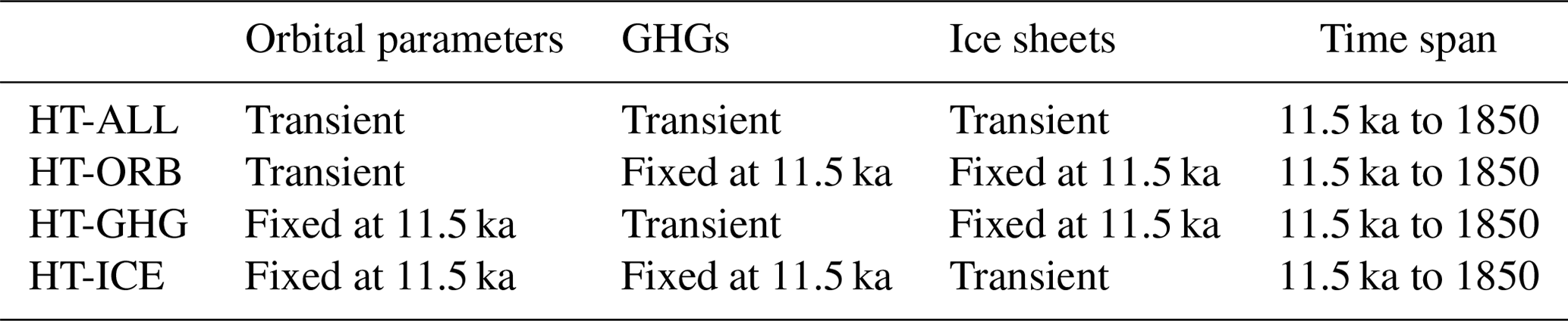
The HT-11.5 ka simulations of the Holocene focus on the period from 11.5 ka to the preindustrial period (1850), which will be the supplement for the PMIP4 Core simulations of the last deglaciation spanning from 21 to 9 ka (Ivanovic et al., 2016). Note that 0 ka is 1950, and 1850 is equivalent to 0.1 ka. All simulations spin up from the Early Holocene at 11.5 ka, and all boundary conditions are available from 11.5 ka to the preindustrial period. The initialization state at 11.5 ka and boundary conditions since 11.5 ka, including Earth's orbital parameters, atmospheric GHG concentrations, and ice sheets and orography, are summarized in Table 1 and described below. Boundary condition data for the HT-11.5 ka transient experiments are provided on the PMIP4 wiki for the transient deglaciation (PMIP Last Deglaciation Working Group, 2016).
Table 1Summary of model boundary conditions for the Early Holocene (11.5 ka) spin-up and Holocene transient (11.5 ka to 1850) experiments; see the text for details. Data are available from PMIP4 last deglaciation wiki (PMIP Last Deglaciation Working Group, 2016). Boundary condition group headings are in bold. Note: ppm is parts per million and ppb is parts per billion.
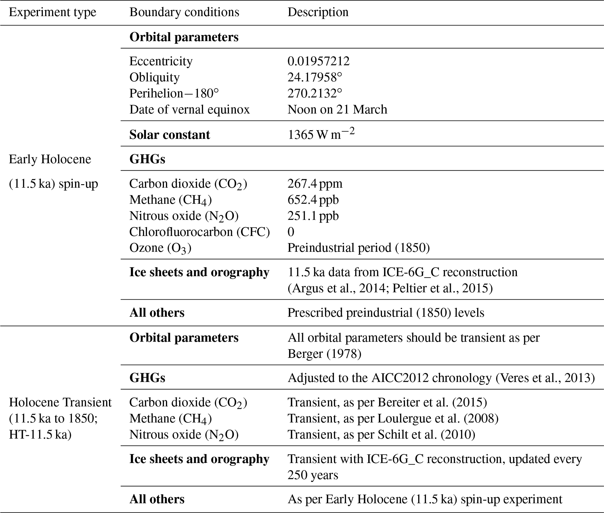
3.1 Early Holocene spin-up
The Early Holocene spin-up experiment for the HT-11.5 ka simulations is an equilibrium or time slice simulation with the boundary conditions of orbital parameters, GHGs, and ice sheets prescribed at 11.5 ka (Table 1). Orbital parameters of eccentricity, obliquity, and longitude of perihelion are set to 0.01957212, 24.17958, and 270.2132∘, respectively, with the date of vernal equinox fixed at the noon on 21 March. The solar constant is fixed to 1365 W m−2, which is consistent with the preindustrial value for the PMIP phase 3 (PMIP3) and CMIP phase 5 (CMIP5) experiments but higher than the value recommended for the transient deglaciation simulation (e.g., 1361.0±0.5 W m−2; Mamajek et al., 2015) and the PMIP4/CMIP6 experiments (e.g., 1360.8±0.5 W m−2; Matthes et al., 2017; Otto-Bliesner et al., 2017). The atmospheric GHGs are prescribed to 267.4 ppm (parts per million) for carbon dioxide (CO2), 652.4 ppb (parts per billion) for methane (CH4), 251.1 ppb for nitrous oxide (N2O), 0 for chlorofluorocarbons (CFCs), and the PMIP3/CMIP5 preindustrial (1850) value for ozone (O3). These values are compatible with the time-evolving boundary conditions for the HT-11.5 ka simulations and consistent with the latest ice core age model (AICC2012; Veres et al., 2013) and records (Loulergue et al., 2008; Schilt et al., 2010; Bereiter et al., 2015). Prescribed ice sheets and the associated topography use the 11.5 ka data from the ICE-6G_C (VM5a) reconstruction (henceforth ICE-6G_C; Argus et al., 2014; Peltier et al., 2015). The initial ocean condition is taken from an archived 500-year spin up (CCSM4; 2∘ resolution in the atmosphere and 1∘ resolution in the ocean and preindustrial control; case b40.1850.track1.2deg.003). All other boundary conditions, such as the coastlines, bathymetry, vegetation and land cover, and aerosols, are prescribed at the preindustrial levels.
Forced by the above boundary conditions, the Early Holocene spin up is continuously integrated for 1500 years, with the absolute value of the trend in global mean surface air and sea surface temperatures being less than 0.05 ∘C and the Atlantic Meridional Overturning Circulation being stable (approximately 25.4 Sv) for the last 100 years, which means the model has reached a quasi-equilibrium state, as suggested by Kageyama et al. (2018). All Holocene transient experiments start from this equilibrium state at 11.5 ka and run transiently until the preindustrial period at 1850.
3.2 Holocene transient simulations
3.2.1 Orbital parameters, solar constant, and insolation anomalies
The Earth's orbital parameters (eccentricity, obliquity, and longitude of perihelion) are time-evolving through the Holocene from 11.5 ka to the preindustrial period, following Berger (1978), which affects the seasonal and latitudinal distribution and magnitude of solar radiation received at the top of the atmosphere. Here, all orbital parameters are interpolated from the originally temporal resolution of 1000 years to 1 year to produce continuous orbital forcings as model inputs. More specifically, the eccentricity declined through the Holocene, indicating a gradual decrease in the seasonal difference of incoming insolation since 11.5 ka. The obliquity was maximal at 9 ka, when the insolation difference was largest between low and high latitudes. The perihelion occurred close to the boreal summer solstice, autumnal equinox, and winter solstice at 11.5, 6 ka, and the preindustrial period, respectively. Due to the above changes, the summer (June–July–August) insolation average in the Northern Hemisphere slightly increased from 465 W m−2 at 11.5 ka to a maximum of 468 W m−2 at about 9.3 ka, and then continuously declined until the preindustrial period. June insolation at 60∘ N gradually decreased through the Holocene, whereas December insolation at 60∘ S increased since 11.5 ka and was maximal around 2 ka (Fig. 1a). Relative to the preindustrial period, June insolation anomalies generally increased with latitude and decreased with time, with positive maximums of ∼50 W m−2 occurring at northern high latitudes during the Early Holocene (Fig. 2).
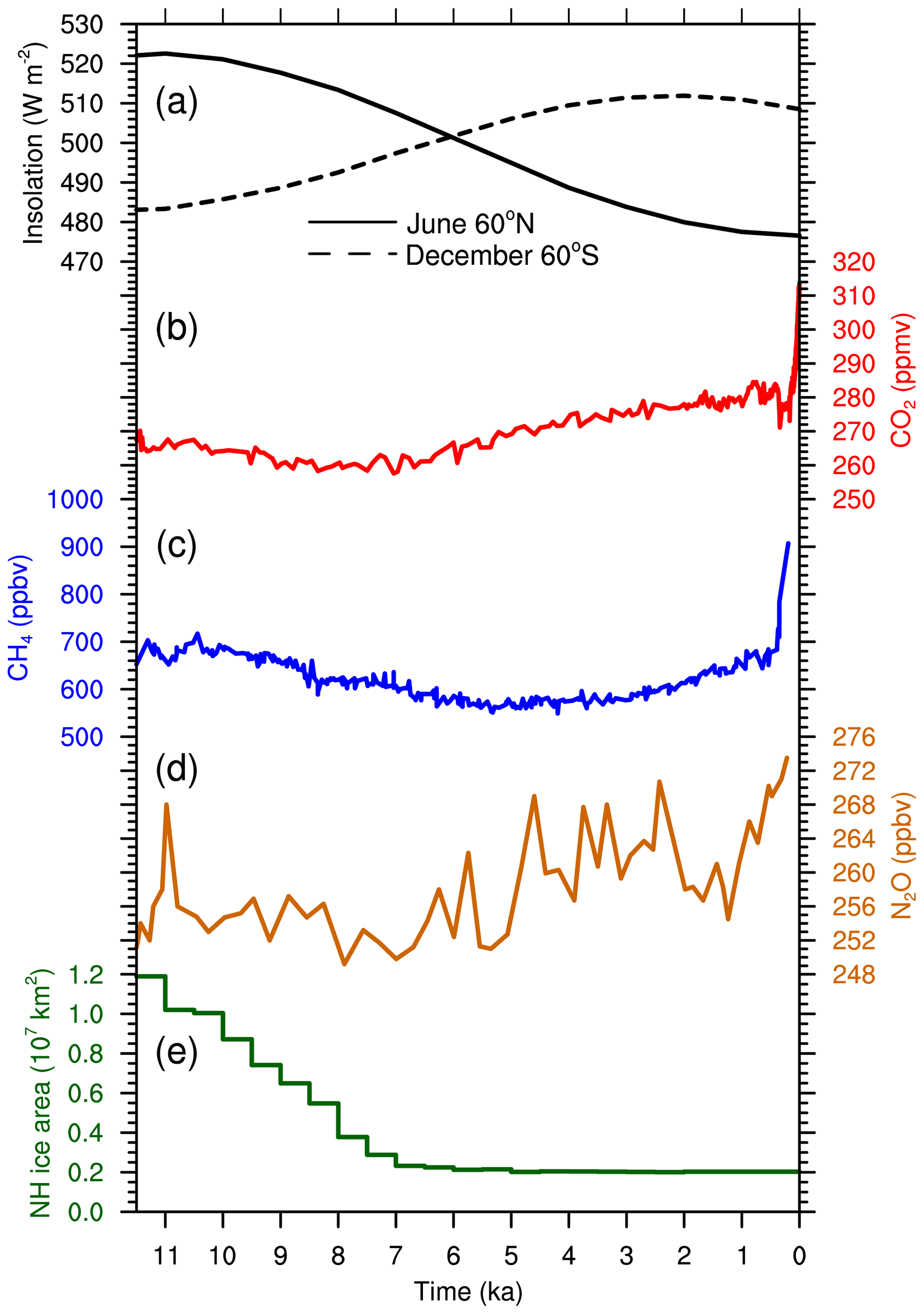
Figure 1Temporal evolution of the external forcings in the HT-11.5 ka simulations since the Early Holocene (11.5 ka), for (a) June insolation at 60∘ N (solid line) and December insolation at 60∘ S (dashed line; Berger, 1978), (b) atmospheric CO2 concentration (recent composite of EPICA Dome C, Law Dome, and West Antarctic Ice Sheet Divide records, Antarctica; Bereiter et al., 2015), (c) atmospheric CH4 concentration (EPICA Dome C, Antarctica; Loulergue et al., 2008), (d) Atmospheric N2O concentration (Talos Dome, Antarctica; Schilt et al., 2010), and (e) area of the ice sheets in the Northern Hemisphere, according to the ICE-6G_C reconstruction (Argus et al., 2014; Peltier et al., 2015).
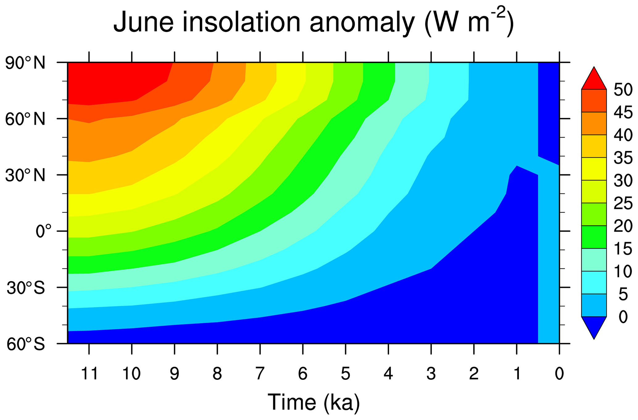
Figure 2Latitude–time anomalies in the June insolation relative to the average for the last 1000 years, according to Berger (1978).
The solar constant is fixed to 1365 W m−2 throughout the run, which is in line with the PMIP3 experiment setup (PMIP PI Working Group, 2010). As mentioned in Otto-Bliesner et al. (2017), this value is higher than the value for the solar constant used by the models in PMIP4 (1360.7 W m−2), which leads to a global increase in incoming solar radiation compared to the PMIP4 experiments.
3.2.2 Atmospheric GHGs
During the Holocene, CFCs is fixed at 0 and O3 is set to the PMIP3/CMIP5 preindustrial value as the Early Holocene spin up. Other atmospheric GHGs are time-evolving through the Holocene and adjusted to the AICC2012 age model (Veres et al., 2013), with CO2 following Bereiter et al. (2015), CH4 following Loulergue et al. (2008), and N2O following Schilt et al. (2010). The high-resolution atmospheric CO2 concentrations are derived from a composite of EPICA Dome C (EDC; Monnin et al., 2001, 2004), the Antarctic composite ice core data built from the Law Dome (MacFarling Meure et al., 2006; Rubino et al., 2013), and the West Antarctic Ice Sheet Divide (Marcott et al., 2014), which show a slightly decreasing trend from 11.5 to 7 ka and an increasing trend afterward (Fig. 1b). The record of atmospheric CH4 concentrations is built from the Antarctic EDC (Loulergue et al., 2008), with a decreasing trend from the Early to Middle Holocene followed by a rising trend (Fig. 1c). The low-resolution atmospheric concentrations of N2O derived from the Talos Dome ice core (Schilt et al., 2010) show large variabilities during the Holocene, with relatively high values around 11 ka and during 6–0 ka but low levels between 11 and 6 ka (Fig. 1d). All the above GHG records are interpolated to the temporal resolution of 1 year to produce continuous forcings as model inputs.
Note that the chronologically accurate values of CO2, CH4, and N2O from the above reconstructions slightly differ from the defined 6 ka concentrations in PMIP4. The nearest measured CO2 concentration to 6 ka is 266.7 ppm from Bereiter et al. (2015), which is higher than the 6 ka value of 264.4 ppm in PMIP4 derived from the original EDC ice core (Monnin et al., 2001, 2004) after a smoothing spline (Otto-Bliesner et al., 2017). In contrast, both the nearest measured CH4 and N2O concentrations of 586 ppb (Loulergue et al., 2008) and 252.4 ppb (Schilt et al., 2010) produced on the AICC2012 chronology (Veres et al., 2013) are lower than the 6 ka values of 597 and 262 ppb in PMIP4 (Otto-Bliesner et al., 2017), respectively, on the original EDC1 chronology (Spahni et al., 2005).
3.2.3 Ice sheets and topography
The ice sheet extent and topography are time-evolving from 11.5 ka to the preindustrial period using the ICE-6G_C reconstruction (Argus et al., 2014; Peltier et al., 2015), which is based on glacial isostatic adjustment modeling and constrained by global positioning system measurements of the vertical motion of the crust, exposure age dating of ice thicknesses, relative sea level histories, and space-based gravity data by the satellite system (Peltier et al., 2015). During the Holocene, the most prominent change in ice sheets occurs in the Northern Hemisphere, especially in North America. According to the ICE-6G_C reconstruction, the North American ice sheet retreated gradually from 11.5 to 9 ka, with the Laurentide ice sheet holding ∼12.5 m global mean sea level rise equivalent ice volume at 10 ka (Matero et al., 2020), retreated sharply from 9 to 7 ka, and almost disappeared after 6 ka (Fig. 3) following the data provided by Dyke (2004). The Eurasian ice sheet has retreated since 11.5 ka and deglaciated after ∼10 ka, following Gyllencreutz et al. (2007), whereas the Greenland ice sheet was stable overall from 11.5 to 9 ka and slightly retreated at its marginal regions during 8–7 ka (Fig. 3). Averaged over the Northern Hemisphere, the ice area continuously declined from km2 at 11.5 ka to km2 during the Middle Holocene (∼7–5 ka) and has remained little changed since then (Fig. 1e). In contrast, there is little variation in the southern hemispheric ice sheets during the Holocene, with only a slight decrease in the ice extent from 11.5 to 10 ka around the Antarctica (Fig. 3). The orography evolves to be consistent with the ice sheet extent, with the elevation of ice sheet below 2000, 2500, and 3500 m over Eurasia, North America, and Greenland, respectively, and reaching 4000 m over Antarctica through the Holocene (Fig. 3). Besides, land surface properties are also adjusted for changes in ice extent. Where ice retreats, land surface is modified to the prescribed vegetation at the preindustrial period.
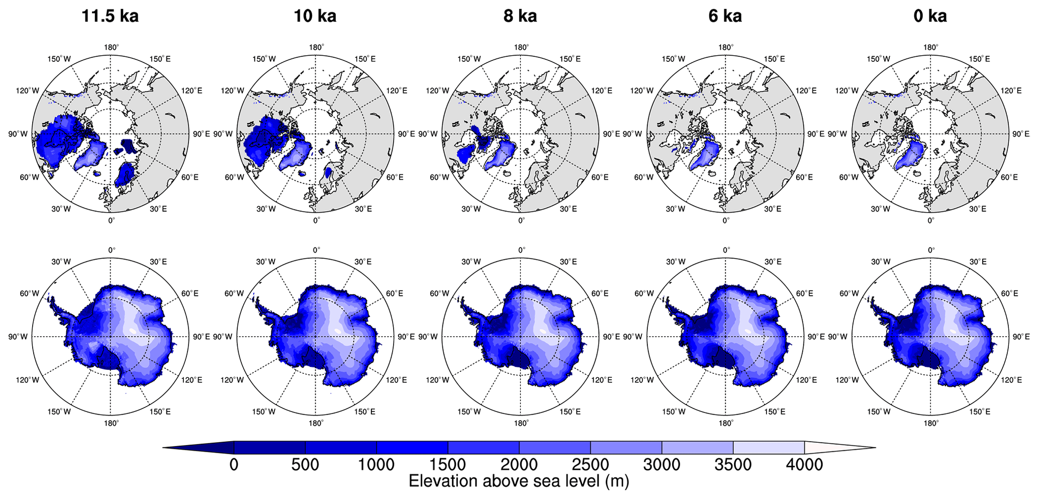
Figure 3Northern Hemisphere (top) and Southern Hemisphere (bottom) ice sheet elevation at 11.5, 10, 8, 6, and 0 ka (1950) for the ICE-6G_C reconstruction at 10 arcmin horizontal resolution; elevation is plotted where the fractional ice mask is more than 0.5 (Peltier et al., 2015).
The original ICE-6G_C data set is provided at 10 arcmin () horizontal resolution and at intervals of 500 years through the Holocene. Both included ice extent and topography data are interpolated to the time interval of 250 years and updated every 250 years in the transient run. Considering that coastlines, bathymetry, and land–sea distributions are little varied during the Holocene, they are fixed as the preindustrial states in all runs. In addition, the meltwater flux change is not considered here, which is one of the options provided for the PMIP4 transient deglaciation experiments. All other forcings, such as the vegetation, land surface, and dust parameters, are prescribed at the preindustrial levels.
3.2.4 Experimental setup
In total, four transient experiments are run in the HT-11.5 ka simulations, namely one all-forcing experiment and three single-forcing experiments. The orbital parameters, atmospheric GHGs, ice sheets and topography, as detailed above, are synchronously evolving with time in the all-forcing experiment (hereinafter HT-ALL), while the three single-forcing experiments are forced by only one of the above forcings, with the other two forcings fixed at 11.5 ka (hereinafter HT-ORB, HT-GHG, and HT-ICE, respectively; Table 2). All four experiments are transiently run from 11.5 ka to the preindustrial period at 1850 for 11.4 kyr. Monthly output data are provided for each simulation.
On the millennium timescale, the annual global mean surface (2 m) air temperature (GMST) in the HT-ALL simulation slightly decreases from 11.5 ka (∼13.20 ∘C) to 7.5 ka (∼12.93 ∘C), with an abrupt cooling at approximately 7.5 ka, and then continuously increases until the preindustrial period (13.57 ∘C; Fig. 4). The warming trend since the Middle Holocene simulated by CESM1.2.1 in our HT-11.5 ka transient experiment is similar to that in the CCSM3, LOVECLIM, and FAMOUS transient simulations (Liu et al., 2014) but opposite to the cooling trend as derived from the multi-proxy reconstructions (Marcott et al., 2013; Kaufman et al., 2020a), which is the so-called Holocene temperature conundrum. The abrupt cooling at approximately 7.5 ka is also seen in the LOVECLIM transient experiment (Liu et al., 2014). In addition, the GMST evolution from Early to Middle Holocene in our CESM1.2.1 transient simulation is somewhat different from the warming trend both in reconstructions and other Holocene transient simulations (Marcott et al., 2013; Liu et al., 2014; Kaufman et al., 2020a), and the reasons for the discrepancies need for further investigation.
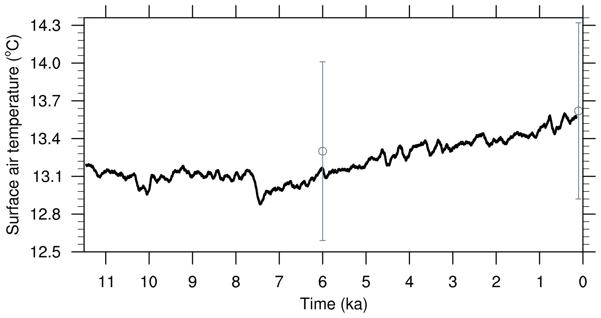
Figure 4Global annual mean surface air temperature since 11.5 ka under the all-forcing simulation. The time series is smoothed by a 101-year moving average. The gray circles at 6 and 0.1 ka stand for the Middle Holocene and preindustrial results simulated by the arithmetic mean of the 14 PMIP4 models, with gray vertical error bars representing plus and minus 1 standard deviation for 14 models.
During the preindustrial period, the annual GMST of 13.57 ∘C in our HT-ALL simulation is very close to that of 13.62 ∘C from the arithmetic mean of the 14 PMIP4 models, although with a spread among the individual models ranging from 12.59 ∘C in IPSL-CM6A-LR to 14.98 ∘C in MIROC-ES2L (Table 3). At 6 ka, the annual GMST is approximately 13.16 ∘C, which resembles the value of 13.30 ∘C from the Middle Holocene simulation in the 14 PMIP4 model arithmetic mean and is within the range from 12.20 ∘C (IPSL-CM6A-LR) to 14.53 ∘C (MIROC-ES2L) in the individual model simulations (Table 3). Relative to the average for 1750–1850, there is a global annual mean cooling of about 0.41 ∘C at 6 ka in the HT-ALL simulation, which lies within the range of the results from the PMIP4 models. In the 14 PMIP4 models, the Middle Holocene cooling varied from 0.18 ∘C in FGOALS-g3 to 0.49 ∘C in FGOALS-f3-L with respect to the preindustrial period, with a standard deviation of 0.11 ∘C among the models and an average of 0.32 ∘C for the arithmetic mean of all models (Fig. 5; Table 3). The geographical distribution of the annual mean surface air temperature change at 6 ka in our HT-ALL simulation is further compared with that from the arithmetic mean of the 14 PMIP4 models (Fig. 6). Compared to the preindustrial period, there is an annual cooling worldwide, except for a slight warming in the high latitudes and over the western Europe, North Pacific, southern North America, and parts of tropical land at 6 ka in the HT-ALL simulation (Fig. 6a). The annual cooling is particularly strong (>1 ∘C) over northern Africa and North America, southern Asia, and part of Southern Ocean. This large-scale distribution is similar to the spatial pattern of the change between the Middle Holocene and preindustrial simulations in the 14 PMIP4 model mean, although some differences exist in magnitude (Fig. 6a, b; Brierley et al., 2020). Quantitatively, the HT-ALL simulation shows an annual cooling of 0.18, 0.40, 0.61, 0.40, 0.31, and 0.20 ∘C at 6 ka averaged for the zonal band of 60–90∘ N, 30–60∘ N, 0–30∘ N, 30∘S–0∘, 60–30∘ S, and 90–60∘ S, respectively. All those values are within the spread of the 14 PMIP4 models, with the largest spread over high latitudes, but are slightly stronger than the cooling in their arithmetic mean by 0.05–0.14 ∘C, especially in the Northern Hemisphere (Fig. 7a). Due to the large seasonal changes in insolation, there are notable seasonal differences in the surface air temperature change at 6 ka, with the December–January–February (DJF) mean change dominating the annual pattern. In response to the decreased insolation in DJF, a strong cooling occurred at 6 ka over the global land regions, especially over the northern continents excluding Greenland, and a weak cooling appeared over the global oceans except for a warming in the Arctic and Southern Ocean (Fig. 6c). In contrast, the increased June–July–August (JJA) insolation at 6 ka led to a notable warming over the northern mid- and high-latitude continents, a weak warming over the northern mid- and high-latitude oceans and southern continents, and a cooling in the other regions (Fig. 6e). The seasonal difference in the spatial distribution of the surface air temperature changes at 6 ka in the HT-ALL simulation resembles that for the Middle Holocene simulations in most PMIP4 models and their arithmetic mean (Fig. 6d, f; Brierley et al., 2020). In a quantitative manner, the HT-ALL simulation shows a consistent DJF cooling of 0.68 (0.31), 0.95 (0.22), and 0.83 (0.43) ∘C averaged over the 30∘ zonal band of northern (southern) high-, mid-, and low-latitudes, respectively (Fig. 7b). For JJA, it displays an average warming of 0.99 and 0.50 ∘C over the northern high- and mid-latitudes but an average cooling varying from 0.41 to 0.66 ∘C over the other four zonal bands (Fig. 7c). On average, there is a global mean cooling of 0.60 for DJF and 0.17 ∘C for JJA (Table 3). All those zonal and global mean changes in seasonal temperatures are within the range of the Middle Holocene changes in the 14 PMIP4 models, which are consistent with the changes from the 14 PMIP4 model arithmetic mean in signs but overall larger than the latter in magnitudes (Fig. 7b and c and Table 3). More specifically, both PMIP4 model spreads and differences of zonal mean changes between the HT-ALL and 14 PMIP4 model mean simulations are largest at northern high latitudes in DJF and at high latitudes in both hemispheres in JJA. As a whole, both at global and zonal mean scales, the annual and seasonal mean changes in surface air temperature at 6 ka in our HT-ALL simulation lie within the range of the 14 PMIP4 model results and are overall stronger than their arithmetic means. In particular, the annual, DJF, and JJA mean GMSTs simulated by CESM1.2.1 in the HT-ALL simulation are lower than those by CESM2 in the PMIP4 both for 6 ka and preindustrial simulations (Table 3). However, the Middle Holocene annual and DJF cooling magnitudes simulated by CESM1.2.1 (0.41 and 0.60 ∘C) are nearly double those in CESM2 (0.20 and 0.38 ∘C), and the JJA cooling in the former (−0.17 ∘C) is opposite to and 4 times the JJA warming in the latter (0.04 ∘C; Table 3). There are also some differences, mainly in magnitudes, for the zonal mean changes in annual and seasonal temperatures at 6 ka between the two versions of CESM (Fig. 7).
Table 3Global annual, DJF, and JJA mean surface air temperatures (units in ∘C) for the preindustrial period, Middle Holocene, and the difference between the Middle Holocene and preindustrial periods in simulations from the 14 PMIP4 models, their arithmetic mean (MMM), and HT-ALL. In the HT-ALL simulation, the preindustrial and Middle Holocene refers to the average for 1750–1850 and 6 ka ± 0.05 ka, respectively.
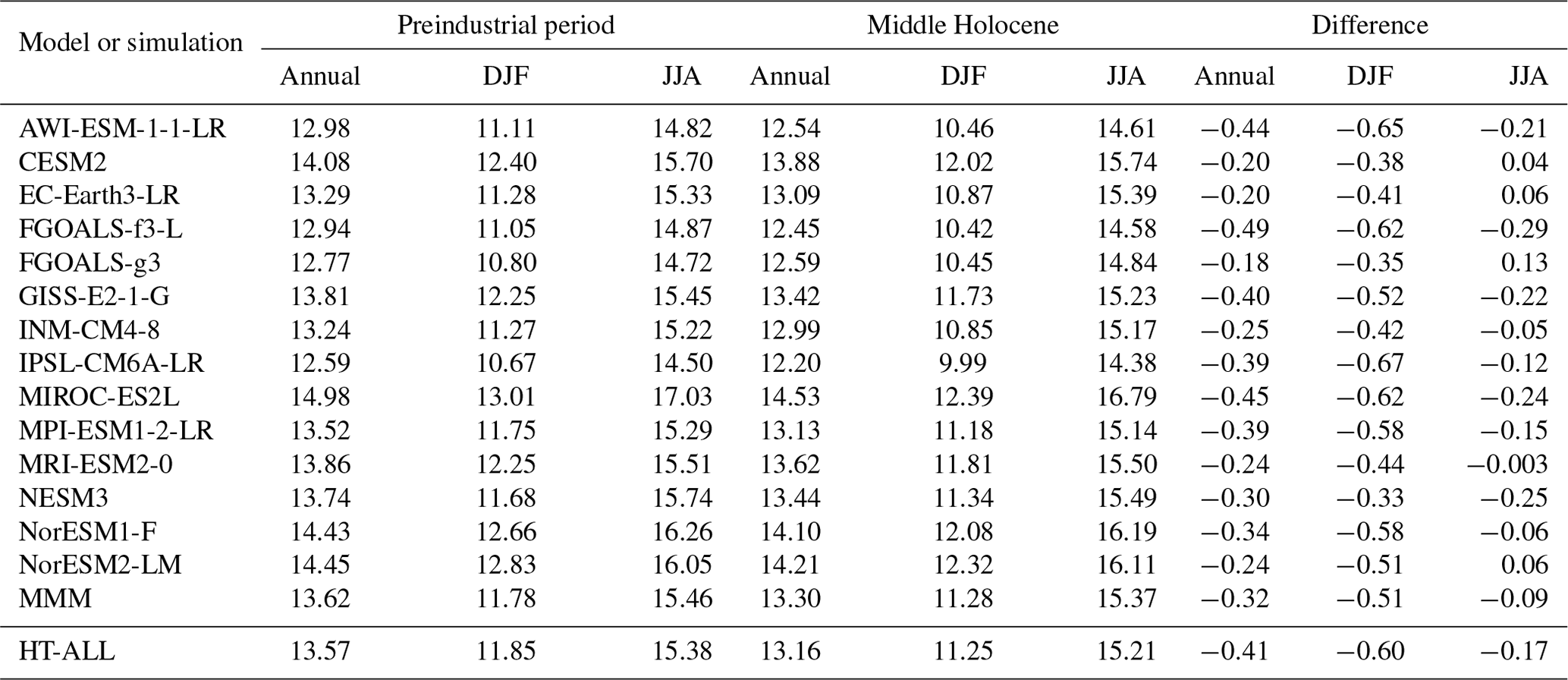
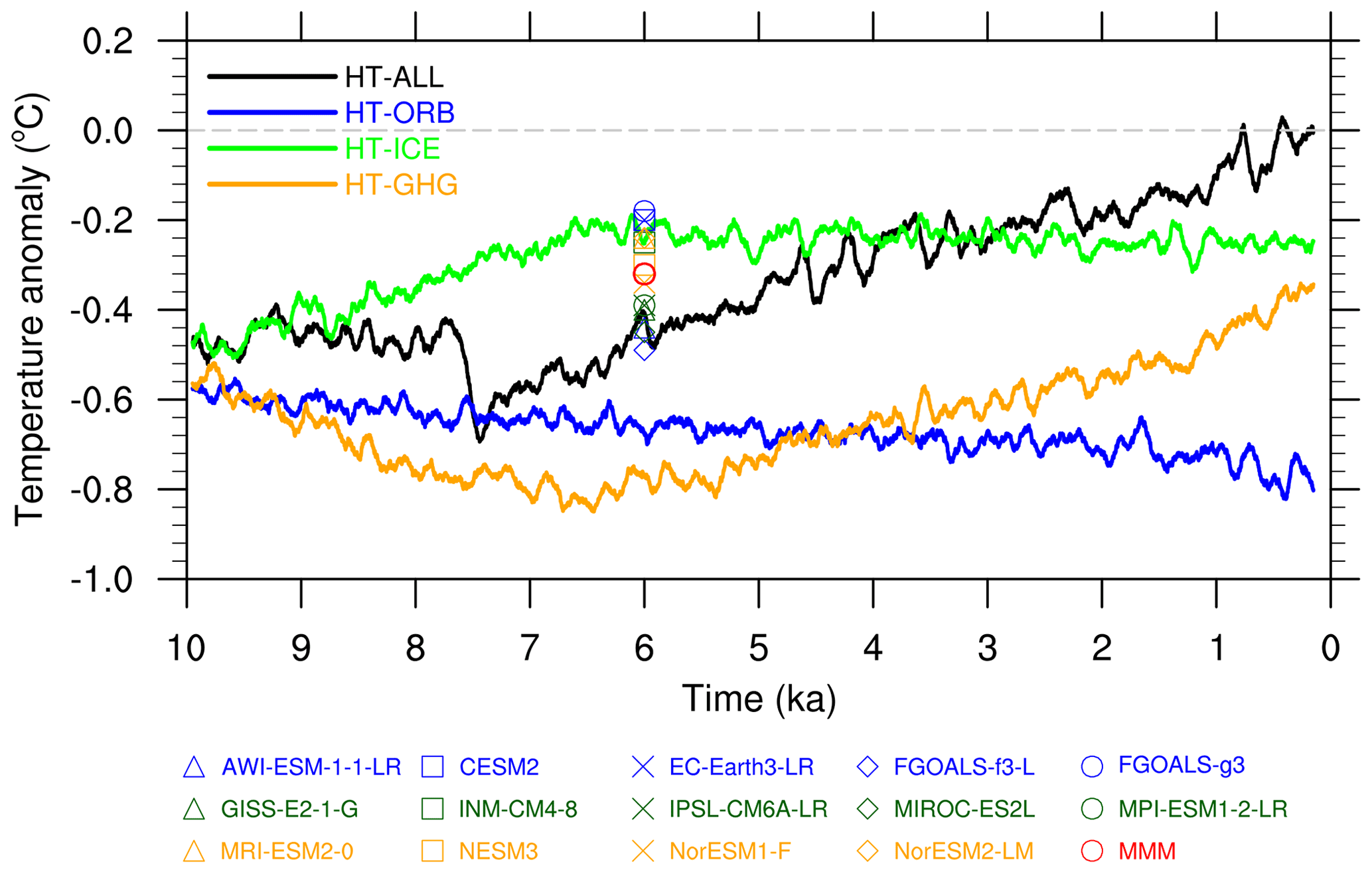
Figure 5Global annual mean surface air temperature anomaly since 10 ka under the all-forcing (HT-ALL – black) and the single-forcing (HT-ORB – blue; HT-ICE – green; HT-GHG – orange) simulations relative to the last 101 years of the all-forcing simulation. All of the time series are smoothed by a 101-year moving average. The triangle, square, cross, diamond, and circle symbols at 6 ka stand for the Middle Holocene minus preindustrial results simulated by the 14 PMIP4 models and their multimodel arithmetic mean (MMM).
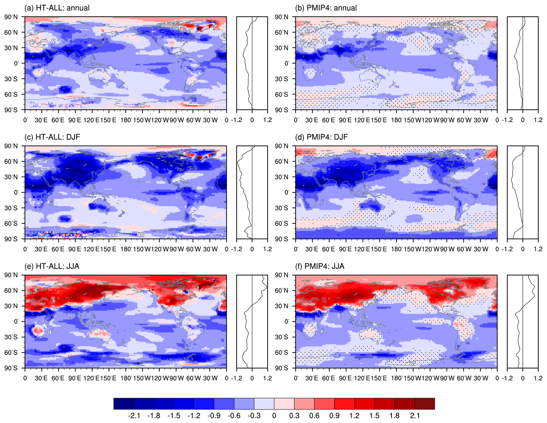
Figure 6Changes in (a, b) annual, (c, d) DJF, and (e, f) JJA mean surface air temperatures (units in ∘C) (a, c, e) between the averages for 6 ka ± 0.05 ka and the last 101 years (i.e., 1750–1850) in the HT-ALL simulation and (b, d, f) between the Middle Holocene and preindustrial simulations in the arithmetic mean of the 14 PMIP4 models, as listed in Fig. 5. The zonal mean changes are shown on the right of each panel. The dotted areas in (b), (d), and (f) represent less than 70 % of the PMIP4 models agree with the sign of multimodel mean change.
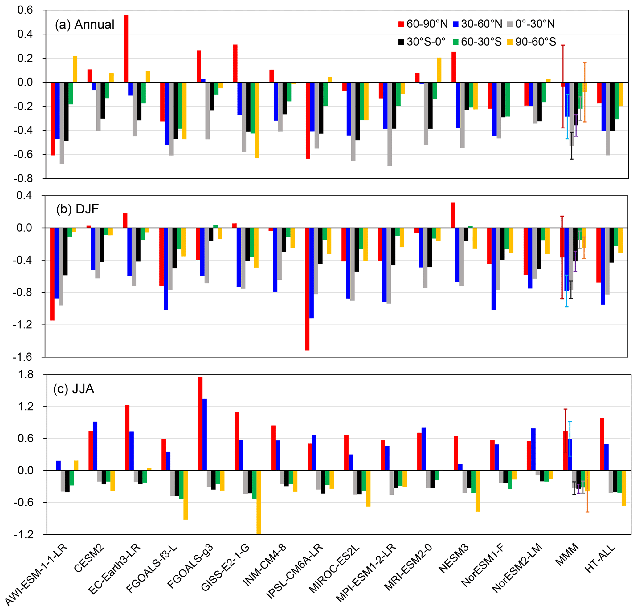
Figure 7Zonal averaged changes in (a) annual, (b) DJF, and (c) JJA mean surface air temperatures (units in ∘C) between the Middle Holocene and preindustrial simulations in the 14 PMIP4 models and their arithmetic mean (MMM), as well as between the averages for 6 ka ± 0.05 ka and the last 101 years (i.e., 1750–1850) in the HT-ALL simulation. Red, blue, gray, black, green, and orange bars represent the changes averaged over the zonal bands of 60–90∘ N, 30–60∘ N, 0∘–30∘ N, 30∘ S–0∘, 60–30∘ S, and 90–60∘ S, respectively. The error bar for the multimodel mean change represents plus and minus 1 standard deviation for the 14 PMIP4 models.
Figure 5 further displays the annual GMST evolution since 10 ka in the all-forcing and single-forcing simulations. All time series are the anomalies relative to the last 101 years (1750–1850) of the HT-ALL simulation. In response to the orbital forcing alone, the GMST slightly decreases during the past 10 ka, with an averaged cooling of approximately 0.2 ∘C in the HT-ORB simulation. The GMST first decreases from 10 to 6.5 ka and then steadily increases until now in the HT-GHG simulation, which closely follows the evolution of the atmospheric concentration of CO2 and is also modulated by that of CH4 and N2O. In the HT-ICE simulation, the GMST increases from 10 to 6 ka in response to the retreat of ice sheets in the Northern Hemisphere and then slightly decreases possibly due to the lag effect of ice sheet melting. Taken together, the weak cooling trend during the Early Holocene in the HT-ALL simulation is mainly driven by both changes in orbital insolation and GHG concentrations, while the retreat of ice sheets plays an opposite role. On the other hand, the strong warming trend since 7.5 ka is mainly induced by increased concentrations of GHGs, which largely results from that of CO2, with a simultaneously positive contribution from the retreat of ice sheets during 7.5–6 ka and a negative contribution from the orbital insolation throughout the past 7.5 ka. It is worth mentioning that, relative to the average for 1750–1850 in the HT-ALL experiment, the annual GMST anomalies since 10 ka in the three single-forcing experiments do not sum to the anomaly in the all-forcing experiment in our HT-11.5 ka simulations (Fig. 5), which holds true for the single- and all-forcing experiments in the CCSM3, LOVECLIM, and FAMOUS transient simulations (Smith and Gregory, 2012; Liu et al., 2014) and indicates a level of nonlinearity in the climate system.
The Holocene presents a host of opportunities to study the climate evolution over the latest interglacial period, including the mean climate trend on the millennium scale and abrupt changes on the timescales from decades to centuries. The climate model provides a useful tool to investigate the underlying dynamic mechanism for the climate change during this well-reconstructed time period; in particular, the improvements of the model and computational power make it possible to run transient simulations to comprehensively understand the climate evolution in response to time-varying external forcings and feedbacks. Several modeling studies have begun this work, but most of them are performed with climate system models or Earth system models with low spatial resolutions and/or acceleration techniques to reduce computational resources. Therefore, we have carried out a new set of unaccelerated transient experiments covering the whole Holocene since 11.5 ka (HT-11.5 ka), using a comprehensive Earth system model with relatively high spatial resolutions, considering both the full-forcing and single-forcing effects of the main boundary conditions.
The HT-11.5 ka simulations are run with the NCAR CESM1.2.1 with an atmospheric resolution of approximately in the horizontal and 26 layers in the vertical and an oceanic resolution of approximately 1∘ and 60 levels in the horizontal and vertical, respectively. All simulations are spin up from the Early Holocene at 11.5 ka and transiently run from 11.5 ka to the preindustrial period at 1850, with the boundary conditions of Earth's orbital parameters, atmospheric GHGs, and ice sheets and orography that have been provided on the PMIP4 wiki for the transient deglaciation (PMIP Last Deglaciation Working Group, 2016). In total, four transient experiments are run, namely one all-forcing experiment forced by synchronously time-evolving orbital parameters, atmospheric GHGs, and ice sheets and three single-forcing experiments forced by only one of the above forcings with the other two forcings fixed at 11.5 ka. The all-forcing simulation result shows a slight decrease in the annual GMST from 11.5 to 7.5 ka, due to both changes in orbital insolation and GHG concentrations, with an abrupt cooling at approximately 7.5 ka, which is followed by a continuous warming until the preindustrial period, mainly resulting from increased GHG concentrations. Relative to the preindustrial period, both at global and zonal mean scales, the simulated annual and seasonal mean changes in surface air temperature at 6 ka are within the range of values in the 14 PMIP4 model simulations and overall stronger than those from their arithmetic mean. The Late Holocene warming trend simulated by CESM1.2.1 in our all-forcing simulation is consistent with that in the CCSM3, LOVECLIM, and FAMOUS transient simulations, as shown in Liu et al. (2014), but inconsistent with the reconstructed cooling trend in Marcott et al. (2013) and Kaufman et al. (2020a).
The present HT-11.5 ka transient simulations for the whole Holocene, spanning from 11.5 ka to the preindustrial period, are designed to investigate both combined and separated effects of the main external forcing of orbital insolation, atmospheric GHGs, and ice sheets on the climate evolution over the Holocene, which will be the supplement for the PMIP4 transient Core experiments for the last deglaciation from 21 to 9 ka (Ivanovic et al., 2016) and the PMIP4 Tier 3 transient simulations for the Holocene from 6 to 0 ka (Otto-Bliesner et al., 2017). Although this new set of transient Holocene simulations are run with a high-resolution version of the comprehensive Earth system model, the meltwater flux change, solar irradiance and volcanic forcing, land use and vegetation changes, dust and aerosol effects, and stratospheric chemistry and dynamics are not fully considered here, which will have some effects on the results. As a first step, this study provides the detailed model description, experimental design, boundary conditions, and some preliminary results for the new set of HT-11.5 ka transient simulations. Further analyses on the simulation results, including the mean climate evolution and abrupt climate changes over the Holocene both at global and regional scales, the underlying dynamic mechanisms, and comparisons with other transient simulations covering the Holocene and multi-proxy-based reconstructions, will be carried out by a series of follow-up studies.
All boundary condition data required for running the HT-11.5 ka experiments (summarized in Tables 1 and 2) can be downloaded from the PMIP4 last deglaciation wiki (PMIP Last Deglaciation Working Group, 2016). The CESM1.2.1 source code is available from the CESM official website (CESM Climate Modeling Group, 2013). The initial ocean condition for the Early Holocene spin-up experiment is obtained from NCAR model case (b40.1850.track1.2deg.003) and is available from the CCSM4 input data archive (CCSM4 Climate Modeling Group, 2011). The PMIP4 model output for the Middle Holocene and preindustrial experiments can be downloaded via the Earth System Grid Federation (ESGF; https://esgf-node.llnl.gov/search/cmip6/, last access: 20 February 2022). The GMST data from the HT-11.5 ka transient simulation shown in this study can be accessed at https://zenodo.org/record/6269566#.Yhg79OhBxLo (last access: 25 February 2022) and are archived at https://doi.org/10.5281/zenodo.6269566 (Tian et al., 2022). Other HT-11.5 ka transient simulation data are available upon reasonable request to the first author and can also be reproduced with the above code and boundary condition data.
DJ conceived the idea and designed the HT-11.5 ka experiments. BS collected all boundary condition data for the simulations, debugged the CESM1.2.1 model, and performed the Early Holocene spin-up, the all-forcing transient simulation, and the initial run of the three single-forcing transient simulations. RZ contributed to the rest run of the three single-forcing transient simulations. ZT wrote the paper, processed the output data from all simulations, and produced the figures, with contributions from all authors.
The contact author has declared that neither they nor their co-authors have any competing interests.
Publisher’s note: Copernicus Publications remains neutral with regard to jurisdictional claims in published maps and institutional affiliations.
We are grateful to the two anonymous reviewers, for their insightful comments and suggestions to improve this work, to the NCAR CESM and PMIP4 climate modeling groups, for producing and sharing their model source code and model output, and to Jean-Yves Peterschmitt (Laboratoire des Sciences du Climat et de l'Environnement, France), for managing and archiving the boundary conditions for the transient deglaciation experiment and setting up and maintaining the PMIP4 last deglaciation wiki pages.
This research has been supported by the National Key Research and Development Program of China (grant no. 2017YFA0603404), the Strategic Priority Research Program of Chinese Academy of Sciences (grant no. XDA20070103), and the National Natural Science Foundation of China (grant nos. 41931181 and 42075048).
This paper was edited by Riccardo Farneti and reviewed by two anonymous referees.
An, Z., Porter, S. C., Kutzbach, J. E., Wu, X., Wang, S., Liu, X., Li, X., and Zhou, W.: Asynchronous Holocene optimum of the East Asian monsoon, Quaternary Sci. Rev., 19, 743–762, https://doi.org/10.1016/S0277-3791(99)00031-1, 2000.
Argus, D. F., Peltier, W. R., Drummond, R., and Moore, A. W.: The Antarctica component of postglacial rebound model ICE-6G_C (VM5a) based on GPS positioning, exposure age dating of ice thicknesses, and relative sea level histories, Geophys. J. Int., 198, 537–563, https://doi.org/10.1093/gji/ggu140, 2014.
Bader, J., Jungclaus, J., Krivova, N., Lorenz, S., Maycock, A., Raddatz, T., Schmidt, H., Toohey, M., Wu, C.-J., and Claussen, M.: Global temperature modes shed light on the Holocene temperature conundrum, Nat. Commun., 11, 4726, https://doi.org/10.1038/s41467-020-18478-6, 2020.
Baker, J. L., Lachniet, M. S., Chervyatsova, O., Asmerom, Y., and Polyak, V. J.: Holocene warming in western continental Eurasia driven by glacial retreat and greenhouse forcing. Nat. Geosci., 10, 430–435, https://doi.org/10.1038/ngeo2953, 2017.
Bereiter, B., Eggleston, S., Schmitt, J., Nehrbass-Ahles, C., Stocker, T. F., Fischer, H., Kipfstuhl, S., and Chappellaz, J.: Revision of the EPICA Dome C CO2 record from 800 to 600 kyr before present, Geophys. Res. Lett., 42, 542–549, https://doi.org/10.1002/2014GL061957, 2015.
Berger, A.: Long-term variations of daily insolation and Quaternary climatic changes, J. Atmos. Sci., 35, 2362–2367, https://doi.org/10.1175/1520-0469(1978)035<2362:LTVODI>2.0.CO;2, 1978.
Birks, H. H.: South to north: Contrasting late-glacial and early-Holocene climate changes and vegetation responses between south and north Norway, Holocene, 25, 37–52, https://doi.org/10.1177/0959683614556375, 2015.
Bova, S., Rosenthal, Y., Liu, Z., Godad, S. P., and Yan, M.: Seasonal origin for the Holocene and last interglacial thermal maximum, Nature, 589, 548–553, https://doi.org/10.1038/s41586-020-03155-x, 2021.
Braconnot, P., Otto-Bliesner, B., Harrison, S., Joussaume, S., Peterchmitt, J.-Y., Abe-Ouchi, A., Crucifix, M., Driesschaert, E., Fichefet, Th., Hewitt, C. D., Kageyama, M., Kitoh, A., Laîné, A., Loutre, M.-F., Marti, O., Merkel, U., Ramstein, G., Valdes, P., Weber, S. L., Yu, Y., and Zhao, Y.: Results of PMIP2 coupled simulations of the Mid-Holocene and Last Glacial Maximum – Part 1: experiments and large-scale features, Clim. Past, 3, 261–277, https://doi.org/10.5194/cp-3-261-2007, 2007.
Braconnot, P., Crétat, J., Marti, O., Balkanski, Y., Caubel, A., Cozic, A., Foujols, M.-A., and Sanogo, S.: Impact of multiscale variability on last 6,000 years Indian and West African monsoon rain, Geophys. Res. Lett., 46, 14021–14029, https://doi.org/10.1029/2019GL084797, 2019a.
Braconnot, P., Zhu, D., Marti, O., and Servonnat, J.: Strengths and challenges for transient Mid- to Late Holocene simulations with dynamical vegetation, Clim. Past, 15, 997–1024, https://doi.org/10.5194/cp-15-997-2019, 2019b.
Brierley, C. M., Zhao, A., Harrison, S. P., Braconnot, P., Williams, C. J. R., Thornalley, D. J. R., Shi, X., Peterschmitt, J.-Y., Ohgaito, R., Kaufman, D. S., Kageyama, M., Hargreaves, J. C., Erb, M. P., Emile-Geay, J., D'Agostino, R., Chandan, D., Carré, M., Bartlein, P. J., Zheng, W., Zhang, Z., Zhang, Q., Yang, H., Volodin, E. M., Tomas, R. A., Routson, C., Peltier, W. R., Otto-Bliesner, B., Morozova, P. A., McKay, N. P., Lohmann, G., Legrande, A. N., Guo, C., Cao, J., Brady, E., Annan, J. D., and Abe-Ouchi, A.: Large-scale features and evaluation of the PMIP4-CMIP6 midHolocene simulations, Clim. Past, 16, 1847–1872, https://doi.org/10.5194/cp-16-1847-2020, 2020.
Brooks, S. J., Matthews, I. P., Birks, H. H., and Birks, H. J. B.: High resolution Lateglacial and early-Holocene summer air temperature records from Scotland inferred from chironomid assemblages, Quaternary Sci. Rev., 41, 67–82, https://doi.org/10.1016/j.quascirev.2012.03.007, 2012.
Carré, M., Braconnot, P., Elliot, M., d'Agostino, R., Schurer, A., Shi, X., Marti, O., Lohmann, G., Jungclaus, J., Cheddadi, R., di Carlo, I. A., Cardich, J., Ochoa, D., Gismondi, R. S., Pérez, A., Romero, P. E., Turcq, B., Corrège, T., and Harrison, S. P.: High-resolution marine data and transient simulations support orbital forcing of ENSO amplitude since the mid-Holocene, Quaternary Sci. Rev., 268, 107125, https://doi.org/10.1016/j.quascirev.2021.107125, 2021.
CCSM4 Climate Modeling Group: CCSM4 input data, Subversion [data set], https://svn-ccsm-inputdata.cgd.ucar.edu/trunk/inputdata/ccsm4_init/b40.1850.track1.2deg.003/0501-01-01/ (last access: 5 May 2022), 2011.
CESM Climate Modeling Group: CESM1.2.1 release code, Subversion [code], https://svn-ccsm-models.cgd.ucar.edu/cesm1/release_tags/cesm1_2_1 (last access: 20 February 2022), 2013.
Chen, F., Yu, Z., Yang, M., Ito, E., Wang, S., Madsen, D. B., Huang, X., Zhao, Y., Sato, T., Birks, H. J. B., Boomer, I., Chen, J., An, C., and Wünnemann, B.: Holocene moisture evolution in arid central Asia and its out-of-phase relationship with Asian monsoon history, Quaternary Sci. Rev., 27, 351–364, https://doi.org/10.1016/j.quascirev.2007.10.017, 2008.
Chen, F., Chen, J., Huang, W., Chen, S., Huang, X., Jin, L., Jia, J., Zhang, X., An, C., Zhang, J., Zhao, Y., Yu, Z., Zhang, R., Liu, J., Zhou, A., and Feng, S.: Westerlies Asia and monsoonal Asia: spatiotemporal differences in climate change and possible mechanisms on decadal to sub-orbital timescales, Earth-Sci. Rev., 192, 337–354, https://doi.org/10.1016/j.earscirev.2019.03.005, 2019.
Craig, A. P., Vertenstein, M., and Jacob, R.: A new flexible coupler for earth system modeling developed for CCSM4 and CESM1, Int. J. High Perform. C., 26, 31–42, https://doi.org/10.1177/1094342011428141, 2012.
Crétat, J., Braconnot, P., Terray, P., Marti, O., and Falasca, F.: Mid-Holocene to present-day evolution of the Indian monsoon in transient global simulations, Clim. Dyn., 55, 2761–2784, https://doi.org/10.1007/s00382-020-05418-9, 2020.
Dallmeyer, A., Claussen, M., Lorenz, S. J., and Shanahan, T.: The end of the African humid period as seen by a transient comprehensive Earth system model simulation of the last 8000 years, Clim. Past, 16, 117–140, https://doi.org/10.5194/cp-16-117-2020, 2020.
Dallmeyer, A., Claussen, M., Lorenz, S. J., Sigl, M., Toohey, M., and Herzschuh, U.: Holocene vegetation transitions and their climatic drivers in MPI-ESM1.2, Clim. Past, 17, 2481–2513, https://doi.org/10.5194/cp-17-2481-2021, 2021.
Danabasoglu, G., Bates, S. C., Briegleb, B. P., Jayne, S. R., Jochum, M., Large, W. G., Peacock, S., and Yeager, S. G.: The CCSM4 ocean component, J. Clim., 25, 1361–1389, https://doi.org/10.1175/JCLI-D-11-00091.1, 2012.
Deevey, E. S. and Flint, R. F.: Postglacial hypsithermal interval, Science, 125, 182–184, https://doi.org/10.1126/science.125.3240.182, 1957.
Dyke, A. S.: An outline of North American deglaciation with emphasis on central and northern Canada, in: Quaternary Glaciations-Extent and Chronology – Part II: North America, vol. 2, Part 2, 371–406, Elsevier, https://www.lakeheadu.ca/sites/default/files/uploads/53/outlines/2014-15/NECU5311/Dyke_2004_DeglaciationOutline.pdf (last access: 20 November 2021), 2004.
Eyring, V., Bony, S., Meehl, G. A., Senior, C. A., Stevens, B., Stouffer, R. J., and Taylor, K. E.: Overview of the Coupled Model Intercomparison Project Phase 6 (CMIP6) experimental design and organization, Geosci. Model Dev., 9, 1937–1958, https://doi.org/10.5194/gmd-9-1937-2016, 2016.
Gasse, F.: Hydrological changes in Africa, Science, 292, 2259–2260, https://doi.org/10.1126/science.1061940, 2001.
Gent, P. R., Danabasoglu, G., Donner, L. J., Holland, M. M., Hunke, E. C., Jayne, S. R., Lawrence, D. M., Neale, R. B., Rasch, P. J., Vertenstein, M., Worley, P. H., Yang, Z.-L., and Zhang, M.: The Community Climate System Model version 4, J. Clim., 24, 4973–4991, https://doi.org/10.1175/2011JCLI4083.1, 2011.
Goldner, A., Herold, N., and Huber, M.: The challenge of simulating the warmth of the mid-Miocene climatic optimum in CESM1, Clim. Past, 10, 523–536, https://doi.org/10.5194/cp-10-523-2014, 2014.
Goosse, H., Brovkin, V., Fichefet, T., Haarsma, R., Huybrechts, P., Jongma, J., Mouchet, A., Selten, F., Barriat, P.-Y., Campin, J.-M., Deleersnijder, E., Driesschaert, E., Goelzer, H., Janssens, I., Loutre, M.-F., Morales Maqueda, M. A., Opsteegh, T., Mathieu, P.-P., Munhoven, G., Pettersson, E. J., Renssen, H., Roche, D. M., Schaeffer, M., Tartinville, B., Timmermann, A., and Weber, S. L.: Description of the Earth system model of intermediate complexity LOVECLIM version 1.2, Geosci. Model Dev., 3, 603–633, https://doi.org/10.5194/gmd-3-603-2010, 2010.
Gordon, C., Cooper, C., Senior, C. A., Banks, H., Gregory, J. M., Johns, T. C., Mitchell, J. F. B., and Wood, R. A.: The simulation of SST, sea ice extents and ocean heat transports in a version of the Hadley Centre coupled model without flux adjustments, Clim. Dyn., 16, 147–168, https://doi.org/10.1007/s003820050010, 2000.
Gupta, A. K., Anderson, D. M., and Overpeck, J. T.: Abrupt changes in the Asian southwest monsoon during the Holocene and their links to the North Atlantic Ocean, Nature, 421, 354–357, https://doi.org/10.1038/nature01340, 2003.
Gyllencreutz, R., Mangerud, J., Svendsen, J.-I., and Lohne, Ø.: DATED – a GIS-based reconstruction and dating database of the Eurasian deglaciation, Appl. Quaternary Res. Cent. Part Glaciat. Terrain Geol. Surv. Finl. Spec. Pap., 46, 113–120, 2007.
Hald, M., Andersson, C., Ebbesen, H., Jansen, E., Klitgaard-Kristensen, D., Risebrobakken, B., Salomonsen, G. R., Sarnthein, M., Sejrup, H. P., and Telford, R. J.: Variations in temperature and extent of Atlantic Water in the northern North Atlantic during the Holocene, Quaternary Sci. Rev., 26, 3423–3440, https://doi.org/10.1016/j.quascirev.2007.10.005, 2007.
Harrison, S., Bartlein, P., Izumi, K., Li, G., Annan, J., Hargreaves, J., Braconnot, P., and Kageyama, M.: Evaluation of CMIP5 palaeo-simulations to improve climate projections, Nat. Clim. Change, 5, 735–743, https://doi.org/10.1038/nclimate2649, 2015.
Haug, G. H., Hughen, K. A., Sigman, D. M., Peterson, L. C., and Röhl, U.: Southward migration of the Intertropical Convergence Zone through the Holocene, Science, 293, 1304–1308, https://doi.org/10.1126/science.1059725, 2001.
He, F.: Simulating transient climate evolution of the last deglaciation with CCSM3, PhD thesis, University of Wisconsin-Madison, 161 pp., 2011.
Hoelzmann, P., Gasse, F., Dupont, L. M., Salzmann, U., Staubwasser, M., Leuschner, D. C., and Sirocko, F.: Palaeoenvironmental changes in the arid and sub arid belt (Sahara-Sahel-Arabian Peninsula) from 150 kyr to present, in: Past Climate Variability through Europe and Africa, edited by: Battarbee, R. W., Gasse, F., and Stickley, C. E., Springer, Dordrecht, 219–256, https://doi.org/10.1007/978-1-4020-2121-3_12, 2004.
Hunke, E. C. and Lipscomb, W. H.: CICE: The Los Alamos Sea Ice Model, Documentation and Software, version 4.0, Los Alamos National Laboratory, Tech. Rep. LA-CC-06-012, 76 pp., https://www.cesm.ucar.edu/models/cesm1.2/cice/ (last access: 5 June 2022), 2008.
Hurrell, J. W., Holland, M. M., Gent, P. R., Ghan, S., Kay, J. E., Kushner, P. J., Lamarque, J.-F., Large, W. G., Lawrence, D., Lindsay, K., Lipscomb, W. H., Long, M. C., Mahowald, N., Marsh, D. R., Neale, R. B., Rasch, P., Vavrus, S., Vertenstein, M., Bader, D., Collins, W. D., Hack, J. J., Kiehl1, J., and Marshall, S.: The Community Earth System Model: A framework for collaborative research, Bull. Amer. Meteorol. Soc., 94, 1339–1360, https://doi.org/10.1175/BAMS-D-12-00121.1, 2013.
IPCC: Climate Change 2021: The Physical Science Basis. Contribution of Working Group I to the Sixth Assessment Report of the Intergovernmental Panel on Climate Change, edited by: Masson-Delmotte, V., Zhai, P., Pirani, A., Connors, S. L., Péan, C., Berger, S., Caud, N., Chen, Y., Goldfarb, L., Gomis, M. I., Huang, M., Leitzell, K., Lonnoy, E., Matthews, J. B. R., Maycock, T. K., Waterfield, T., Yelekçi, O., Yu, R., and Zhou, B., Cambridge University Press, USA, https://www.ipcc.ch/report/ar6/wg1/ (last access: 5 June 2022), in press, 2022.
Ivanovic, R. F., Gregoire, L. J., Kageyama, M., Roche, D. M., Valdes, P. J., Burke, A., Drummond, R., Peltier, W. R., and Tarasov, L.: Transient climate simulations of the deglaciation 21–9 thousand years before present (version 1) – PMIP4 Core experiment design and boundary conditions, Geosci. Model Dev., 9, 2563–2587, https://doi.org/10.5194/gmd-9-2563-2016, 2016.
Jansen, E., Overpeck, J., Briffa, K. R., Duplessy, J. C., Joos, F., Masson-Delmotte, V., Olago, D., Otto-Bliesner, B., Peltier, W. R., Rahmstorf, S., Ramesh, R., Raynaud, D., Rind, D., Solomina, O., Villalba, R., and Zhang, D.: Palaeoclimate, in: Climate Change 2007: The Physical Science Basis. Contribution of Working Group I to the Fourth Assessment Report of the Intergovernmental Panel on Climate Change, edited by: Solomon, S., Qin, D., Manning, M., Chen, Z., Marquis, M., Averyt, K. B., Tignor M., and Miller, H. L., Cambridge University Press, USA, 435–497, https://www.ipcc.ch/site/assets/uploads/2018/02/ar4-wg1-chapter6-1.pdf (last access: 5 June 2022), 2007.
Jin, L., Schneider, B., Park, W., Latif, M., Khon, V., and Zhang, X.: The spatial–temporal patterns of Asian summer monsoon precipitation in response to Holocene insolation change: a model-data synthesis, Quaternary Sci. Rev., 85, 47–62, https://doi.org/10.1016/j.quascirev.2013.11.004, 2014.
Joussaume, S. and Taylor, K. E.: Status of the Paleoclimate Modeling Intercomparison Project (PMIP), in: Proceedings of the First International AMIP Scientific Conference, WCRP report, 425–430, 1995.
Kageyama, M., Braconnot, P., Harrison, S. P., Haywood, A. M., Jungclaus, J. H., Otto-Bliesner, B. L., Peterschmitt, J.-Y., Abe-Ouchi, A., Albani, S., Bartlein, P. J., Brierley, C., Crucifix, M., Dolan, A., Fernandez-Donado, L., Fischer, H., Hopcroft, P. O., Ivanovic, R. F., Lambert, F., Lunt, D. J., Mahowald, N. M., Peltier, W. R., Phipps, S. J., Roche, D. M., Schmidt, G. A., Tarasov, L., Valdes, P. J., Zhang, Q., and Zhou, T.: The PMIP4 contribution to CMIP6 – Part 1: Overview and over-arching analysis plan, Geosci. Model Dev., 11, 1033–1057, https://doi.org/10.5194/gmd-11-1033-2018, 2018.
Kapsch, M.-L., Mikolajewicz, U., Ziemen, F., and Schannwell, C.: Ocean response in transient simulations of the last deglaciation dominated by underlying ice-sheet reconstruction and method of meltwater distribution, Geophys. Res. Lett., 49, e2021GL096767, https://doi.org/10.1029/2021GL096767, 2020.
Kaufman, D., McKay, N., Routson, C., Erb, M., Dätwyler, C., Sommer, P. S., Heiri, O., and Davis, B.: Holocene global mean surface temperature, a multi-method reconstruction approach, Sci. Data, 7, 201, https://doi.org/10.1038/s41597-020-0530-7, 2020a.
Kaufman, D., McKay, N., Routson, C., Erb, M., Davis, B., Heiri, O., Jaccard, S., Tierney, J., Dätwyler, C., Axford, Y., Brussel, T., Cartapanis, O., Chase, B., Dawson, A., de Vernal, A., Engels, S., Jonkers, L., Marsicek, J., Moffa-Sánchez, P., Morrill, C., Orsi, A., Rehfeld, K., Saunders, K., Sommer, P. S., Thomas, E., Tonello, M., Tóth, M., Vachula, R., Andreev, A., Bertrand, S., Biskaborn, B., Bringué, M., Brooks, S., Caniupán, M., Chevalier, M., Cwynar, L., Emile-Geay, J., Fegyveresi, J., Feurdean, A., Finsinger, W., Fortin, M.-C., Foster, L., Fox, M., Gajewski, K., Grosjean, M., Hausmann, S., Heinrichs, M., Holmes, N., Ilyashuk, B., Ilyashuk, E., Juggins, S., Khider, D., Koinig, K., Langdon, P., Larocque-Tobler, I., Li, J., Lotter, A., Luoto, T., Mackay, A., Magyari, E., Malevich, S., Mark, B., Massaferro, J., Montade, V., Nazarova, L., Novenko, E., Pařil, P., Pearson, E., Peros, M., Pienitz, R., Płóciennik, M., Porinchu, D., Potito, A., Rees, A., Reinemann, S., Roberts, S., Rolland, N., Salonen, S., Self, A., Seppä, H., Shala, S., St-Jacques, J.-M., Stenni, B., Syrykh, L., Tarrats, P., Taylor, K., van den Bos, V., Velle, G., Wahl, E., Walker, I., Wilmshurst, J., Zhang, E., and Zhilich, S.: A global database of Holocene paleotemperature records, Sci. Data, 7, 115, https://doi.org/10.1038/s41597-020-0445-3, 2020b.
Kaufman, D. S., Ager, T. A., Anderson, N. J., Anderson, P. M., Andrews, J. T., Bartlein, P. J., Brubaker, L. B., Coats, L. L., Cwynar, L. C., Duvall, M. L., Dyke, A. S., Edwards, M. E., Eisner, W. R., Gajewski, K., Geirsdóttir, A., Hu, F. S., Jennings, A. E., Kaplan, M. R., Kerwin, M. W., Lozhkin, A. V., MacDonald, G. M., Miller, G. H., Mock, C. J., Oswald, W. W., Otto-Bliesner, B. L., Porinchu, D. F., Rühland, K., Smol, J. P., Steig, E. J., and Wolfe, B. B.: Holocene thermal maximum in the western Arctic (0–180∘ W), Quaternary Sci. Rev., 23, 529–560, https://doi.org/10.1016/j.quascirev.2003.09.007, 2004.
Koerner, R. M. and Fisher, D. A.: A record of Holocene summer climate from a Canadian High Arctic ice core, Nature, 343, 630–631, https://doi.org/10.1038/343630a0, 1990.
Kutzbach, J. E., Liu, X., Liu, Z., and Chen, G.: Simulation of the evolutionary response of global summer monsoons to orbital forcing over the past 280 000 years, Clim. Dyn., 30, 567–579, https://doi.org/10.1007/s00382-007-0308-z, 2008.
Lawrence, D. M., Oleson, K. W., Flanner, M. G., Thornton, P. E., Swenson, S. C., Lawrence, P. J., Zeng, X., Yang, Z.-L., Levis, S., Sakaguchi, K., Bonan, G. B., and Slater, A. G.: Parameterization improvements and functional and structural advances in version 4 of the Community Land Model, J. Adv. Model. Earth Sy., 3, M03001, https://doi.org/10.1029/2011MS00045, 2011.
Liu, S., Lang, X., and Jiang, D: Time-varying responses of dryland aridity to external forcings over the last 21 ka, Quaternary Sci. Rev., 262, 106989, https://doi.org/10.1016/j.quascirev.2021.106989, 2021.
Liu, Y., Zhang, M., Liu, Z., Xia, Y., Huang, Y., Peng, Y., and Zhu, J.: A possible role of dust in resolving the Holocene temperature conundrum, Sci. Rep., 8, 4434, https://doi.org/10.1038/s41598-018-22841-5, 2018.
Liu, Z., Zhu, J., Rosenthal, Y., Zhang, X., Otto-Bliesner, B. L., Timmermann, A., Smith, R. S., Lohmann, G., Zheng, W., and Timm, O. E.: The Holocene temperature conundrum, P. Natl. Acad. Sci., 111, E3501–E3505, https://doi.org/10.1073/pnas.1407229111, 2014.
Ljungqvist, F. C.: The spatio-temporal pattern of the mid-Holocene thermal maximum, Geografie, 116, 91–110, https://doi.org/10.37040/geografie2011116020091, 2011.
Loulergue, L., Schilt, A., Spahni, R., Masson-Delmotte, V., Blunier, T., Lemieux, B., Barnola, J.-M., Raynaud, D., Stocker, T. F., and Chappellaz, J.: Orbital and millennial-scale features of atmospheric CH4 over the past 800 000 years, Nature, 453, 383–386, https://doi.org/10.1038/nature06950, 2008.
MacFarling Meure, C., Etheridge, D., Trudinger, C., Steele, P., Langenfelds, R., van Ommen, T., Smith, A., and Elkins, J.: Law Dome CO2, CH4 and N2O ice core records extended to 2000 years BP, Geophys. Res. Lett., 33, L14810, https://doi.org/10.1029/2006GL026152, 2006.
Magny, M., Vannière, B., de Beaulieu, J.-L., Bégeot, C., Heiri, O., Millet, L., Peyron, O., and Walter-Simonnet, A.-V.: Early-Holocene climatic oscillations recorded by lake-level fluctuations in west-central Europe and in central Italy, Quaternary Sci. Rev., 26, 1951–1964, https://doi.org/10.1016/j.quascirev.2006.04.013, 2007.
Mamajek, E. E., Prsa, A., Torres, G., Harmanec, P., Asplund, M., Bennett, P. D., Capitaine, N., Christensen-Dalsgaard, J., Depagne, E., Folkner, W. M., Haberreiter, M., Hekker, S., Hilton, J. L., Kostov, V., Kurtz, D. W., Laskar, J., Mason, B. D., Milone, E. F., Montgomery, M. M., Richards, M. T., Schou, J., and Stewart, S. G.: IAU 2015 Resolution B3 on Recommended Nominal Conversion Constants for Selected Solar and Planetary Properties, ArXiv151007674 Astro-Ph, http://arxiv.org/abs/1510.07674 (last access: 15 November 2021), 2015.
Marcott, S. A., Shakun, J. D., Clark, P. U., and Mix, A. C.: A reconstruction of regional and global temperature for the past 11 300 years, Science, 339, 1198–1201, https://doi.org/10.1126/science.1228026, 2013.
Marcott, S. A., Bauska, T. K., Buizert, C., Steig, E. J., Rosen, J. L., Cuffey, K. M., Fudge, T. J., Severinghaus, J. P., Ahn, J., Kalk, M. L., McConnell, J. R., Sowers, T., Taylor, K. C., White, J. W. C., and Brook, E. J.: Centennial-scale changes in the global carbon cycle during the last deglaciation, Nature, 514, 616–619, https://doi.org/10.1038/nature13799, 2014.
Marsicek, J., Shuman, B. N., Bartlein, P. J., Shafer, S. L., and Brewer, S.: Reconciling divergent trend and millennial variations in Holocene temperatures, Nature, 554, 92–96, https://doi.org/10.1038/nature25464, 2018.
Maslin, M. A. and Burns, S. J.: Reconstruction of the Amazon Basin effective moisture availability over the past 14 000 years, Science, 290, 2285–2287, https://doi.org/10.1126/science.290.5500.2285, 2000.
Matero, I. S. O., Gregoire, L. J., and Ivanovic, R. F.: Simulating the Early Holocene demise of the Laurentide Ice Sheet with BISICLES (public trunk revision 3298), Geosci. Model Dev., 13, 4555–4577, https://doi.org/10.5194/gmd-13-4555-2020, 2020.
Matthes, K., Funke, B., Andersson, M. E., Barnard, L., Beer, J., Charbonneau, P., Clilverd, M. A., Dudok de Wit, T., Haberreiter, M., Hendry, A., Jackman, C. H., Kretzschmar, M., Kruschke, T., Kunze, M., Langematz, U., Marsh, D. R., Maycock, A. C., Misios, S., Rodger, C. J., Scaife, A. A., Seppälä, A., Shangguan, M., Sinnhuber, M., Tourpali, K., Usoskin, I., van de Kamp, M., Verronen, P. T., and Versick, S.: Solar forcing for CMIP6 (v3.2), Geosci. Model Dev., 10, 2247–2302, https://doi.org/10.5194/gmd-10-2247-2017, 2017.
Mayewski, P. A., Rohling, E. E., Stager, J. C., Karlén, W., Maasch, K. A., Meeker, L. D., Meyerson, E. A., Gasse, F., van Kreveld, S., Holmgren, K., Lee-Thorp, J., Rosqvist, G., Rack, F., Staubwasser, M., Schneider, R. R., and Steig, E. J.: Holocene climate variability, Quaternary Res., 62, 243–255, https://doi.org/10.1016/j.yqres.2004.07.001, 2004.
Monnin, E., Indermuhle, A., Dallenbach, A., Fluckiger, J., Stauffer, B., Stocker, T. F., Raynaud, D., and Barnola, J. M.: Atmospheric CO2 concentrations over the last glacial termination, Science, 291, 112–114, https://doi.org/10.1126/science.291.5501.112, 2001.
Monnin, E., Steig, E. J., Siegenthaler, U., Kawamura, K., Schwander, J., Stauffer, B., Stocker, T. F., Morse, D. L., Barnola, J.-M., Bellier, B., Raynaud, D., and Fischer, H.: Evidence for substantial accumulation rate variability in Antarctica during the Holocene, through synchronization of CO2 in the Taylor Dome, Dome C and DML ice cores, Earth Planet. Sci. Lett., 224, 45–54, https://doi.org/10.1016/j.epsl.2004.05.007, 2004.
Neale, R. B., Richter, J. H., Conley, A. J., Park, S., Lauritzen, P. H., Gettelman, A., Williamson, D. L., Rasch, P. J., Vavrus, S. J., Taylor, M. A., Collins, W. D., Zhang, M., and Lin, S.: Description of the NCAR Community Atmosphere Model (CAM 4.0), National Center for Atmospheric Research, Boulder, CO, Tech. Rep. NCAR/TN-485+STR, 194 pp., https://www.cesm.ucar.edu/models/ccsm4.0/cam/docs/description/cam4_desc.pdf (last access: 5 June 2022), 2010.
Nesje, A. and Dahl, S. O.: Lateglacial and Holocene glacier fluctuations and climate variations in western Norway: a review, Quaternary Sci. Rev., 12, 255–261, https://doi.org/10.1016/0277-3791(93)90081-V, 1993.
Núñez, L., Grosjean, M., and Cartajena, I.: Human occupations and climate change in the Puna de Atacama, Chile, Science, 298, 821–824, https://doi.org/10.1126/science.1076449, 2002.
Osman, M. B., Tierney, J. E., Zhu, J., Tardif, R., Hakim, G. J., King, J., and Poulsen, C. J.: Globally resolved surface temperatures since the Last Glacial Maximum, Nature, 599, 239–244, https://doi.org/10.1038/s41586-021-03984-4, 2021.
Otto-Bliesner, B. L., Braconnot, P., Harrison, S. P., Lunt, D. J., Abe-Ouchi, A., Albani, S., Bartlein, P. J., Capron, E., Carlson, A. E., Dutton, A., Fischer, H., Goelzer, H., Govin, A., Haywood, A., Joos, F., LeGrande, A. N., Lipscomb, W. H., Lohmann, G., Mahowald, N., Nehrbass-Ahles, C., Pausata, F. S. R., Peterschmitt, J.-Y., Phipps, S. J., Renssen, H., and Zhang, Q.: The PMIP4 contribution to CMIP6 – Part 2: Two interglacials, scientific objective and experimental design for Holocene and Last Interglacial simulations, Geosci. Model Dev., 10, 3979–4003, https://doi.org/10.5194/gmd-10-3979-2017, 2017.
Park, H.-S., Kim, S.-J., Stewart, A. L., Son, S.-W., and Seo, K.-H.: Mid-Holocene Northern Hemisphere warming driven by Arctic amplification, Sci. Adv., 5, eaax8203, https://doi.org/10.1126/sciadv.aax8203, 2019.
Peltier, W. R., Argus, D. F., and Drummond, R.: Space geodesy constrains ice age terminal deglaciation: The global ICE-6G_C (VM5a) model, J. Geophys. Res.-Sol. Ea., 120, 450–487, https://doi.org/10.1002/2014JB011176, 2015.
PMIP Last Deglaciation Working Group: PMIP4 Last Deglaciation Experiment Design Wiki, PMIP4 [data set], https://pmip4.lsce.ipsl.fr/doku.php/exp_design:degla (last access: 11 November 2021), 2016.
PMIP PI Working Group: PMIP3 Pre-Industrial Control Run Experiment Design, https://wiki.lsce.ipsl.fr/pmip3/doku.php/pmip3:design:pi:index (last access: 16 November 2021), 2010.
Renssen, H., Braconnot, P., Tett, S. F. B., von Storch, H., and Weber, S. L.: Recent developments in Holocene climate modelling, in: Past Climate Variability through Europe and Africa, edited by: Battarbee, R. W., Gasse, F., and Stickley, C. E., Springer, Dordrecht, 495–514, https://doi.org/10.1007/978-1-4020-2121-3_23, 2004.
Renssen, H., Seppä, H., Crosta, X., Goosse, H., Roche, D. M.: Global characterization of the Holocene thermal maximum, Quaternary Sci. Rev., 48, 7–19, https://doi.org/10.1016/j.quascirev.2012.05.022, 2012.
Rubino, M., Etheridge, D. M., Trudinger, C. M., Allison, C. E., Battle, M. O., Langenfelds, R. L., Steele, L. P., Curran, M., Bender, M., White, J. W. C., Jenk, T. M., Blunier, T., and Francey, R. J.: A revised 1000 year atmospheric δ13C-CO2 record from Law Dome and South Pole, Antarctica, J. Geophys. Res.-Atmos., 118, 8482–8499, https://doi.org/10.1002/jgrd.50668, 2013.
Schilt, A., Baumgartner, M., Schwander, J., Buiron, D., Capron, E., Chappellaz, J., Loulergue, L., Schüpbach, S., Spahni, R., Fischer, H., and Stocker, T. F.: Atmospheric nitrous oxide during the last 140 000 years, Earth Planet. Sci. Lett., 300, 33–43, https://doi.org/10.1016/j.epsl.2010.09.027, 2010.
Seltzer, G., Rodbell, D., and Burns, S.: Isotopic evidence for late Quaternary climatic change in tropical South America, Geology, 28, 35–38, https://doi.org/10.1130/0091-7613(2000)28<35:IEFLQC>2.0.CO;2, 2000.
Shakun, J. D., Clark, P. U., He, F., Marcott, S. A., Mix, A. C., Liu, Z., Otto-Bliesner, B., Schmittner, A., and Bard, E.: Global warming preceded by increasing carbon dioxide concentrations during the last deglaciation, Nature, 484, 49–54, https://doi.org/10.1038/nature10915, 2012.
Shevenell, A. E., Ingalls, A. E., Domack, E. W., and Kelly, C.: Holocene Southern Ocean surface temperature variability west of the Antarctic Peninsula, Nature, 470, 250–254, https://doi.org/10.1038/nature09751, 2011.
Shi, X., Werner, M., Krug, C., Brierley, C. M., Zhao, A., Igbinosa, E., Braconnot, P., Brady, E., Cao, J., D'Agostino, R., Jungclaus, J., Liu, X., Otto-Bliesner, B., Sidorenko, D., Tomas, R., Volodin, E. M., Yang, H., Zhang, Q., Zheng, W., and Lohmann, G.: Calendar effects on surface air temperature and precipitation based on model-ensemble equilibrium and transient simulations from PMIP4 and PACMEDY, Clim. Past, 18, 1047–1070, https://doi.org/10.5194/cp-18-1047-2022, 2022.
Shi, Y., Kong, Z., Wang, S., Tang, L., Wang, F., Yao, T., Zhao, X., Zhang, P., and Shi, S.: Mid-Holocene climates and environments in China, Global Planet. Change, 7, 219–233, https://doi.org/10.1016/0921-8181(93)90052-P, 1993.
Sidorenko, D., Goessling, H. F., Koldunov, N. V., Scholz, P., Danilov, S., Barbi, D., Cabos, W., Gurses, O., Harig, S., Hinrichs, C., Juricke, S., Lohmann, G., Losch, M., Mu, L., Rackow, T., Rakowsky, N., Sein, D., Semmler, T., Shi, X., Stepanek, C., Streffing, J., Wang, Q., Wekerle, C., Yang, H., and Jung, T.: Evaluation of FESOM2.0 coupled to ECHAM6.3: preindustrial and HighResMIP simulations, J. Adv. Model. Earth Syst., 11, 3794–3815, https://doi.org/10.1029/2019MS001696, 2019.
Smith, R., Jones, P., Briegleb, B., Bryan, F., Danabasoglu, G., Dennis, J., Dukowicz, J., Eden, C., Fox-Kemper, B., Gent, P., Hecht, M., Jayne, S., Jochum, M., Large, W., Lindsay, K., Maltrud, M., Norton, N., Peacock, S., Vertenstein, M., and Yeager, S.: The Parallel Ocean Program (POP) reference manual, ocean component of the Community Climate System Model (CCSM) and Community Earth System Model (CESM), Los Alamos National Laboratory, Tech. Rep. LAUR-10-01853, 141 pp., https://www.cesm.ucar.edu/models/cesm1.2/pop2/doc/sci/POPRefManual.pdf (last access: 5 June 2022), 2010.
Smith, R. S. and Gregory, J.: The last glacial cycle: transient simulations with an AOGCM, Clim. Dyn., 38, 1545–1559, https://doi.org/10.1007/s00382-011-1283-y, 2012.
Smith, R. S., Gregory, J. M., and Osprey, A.: A description of the FAMOUS (version XDBUA) climate model and control run, Geosci. Model Dev., 1, 53–68, https://doi.org/10.5194/gmd-1-53-2008, 2008.
Solomina, O. N., Bradley, R. S., Hodgson, D. A., Ivy-Ochs, S., Jomelli, V., Mackintosh, A. N., Nesje, A., Owen, L. A., Wanner, H., Wiles, G. C., and Young, N. E.: Holocene glacier fluctuation, Quaternary Sci. Rev., 111, 9–34, https://doi.org/10.1016/j.quascirev.2014.11.018, 2015.
Song, X. and Zhang, G. J.: The roles of convection parameterization in the formation of double ITCZ syndrome in the NCAR CESM: I. Atmospheric processes, J. Adv. Model. Earth Sy., 10, 842–866, https://doi.org/10.1002/2017MS001191, 2018.
Song, X. and Zhang, G. J.: Culprit of the eastern Pacific double ITCZ bias in the NCAR CESM1.2, J. Clim., 32, 6349–6364, https://doi.org/10.1175/JCLI-D-18-0580.1, 2019.
Spahni, R., Chappellaz, J., Stocker, T. F., Loulergue, L., Hausammann, G., Kawamura, K., Flückiger, J., Schwander, J., Raynaud, D., Masson-Delmotte, V., and Jouzel, J.: Atmospheric methane and nitrous oxide of the late Pleistocene from Antarctic ice cores, Science, 310, 1317–1321, https://doi.org/10.1126/science.1120132, 2005.
Staubwasser, M.: An overview of Holocene South Asian monsoon records-monsoon domains and regional contrasts, J. Geolog. Soc. India, 68, 433–446, 2006.
Sun, W., Liu, J., Wan, L., Ning, L., and Yan, M.: Simulation of Northern Hemisphere mid-latitude precipitation response to different external forcings during the Holocene (in Chinese), Quaternary Sci., 40, 1588–1596, https://doi.org/10.11928/j.issn.1001-7410.2020.06.18, 2020.
Taylor, K. E., Stouffer, R. J., and Meehl G. A.: An overview of CMIP5 and the experiment design, Bull. Amer. Meteorol. Soc., 93, 485–498, https://doi.org/10.1175/BAMS-D-11-00094.1, 2012.
Tian, Z., Jiang, D., Zhang, R., and Su, B.: HT-11.5 ka transient simulation data of GMST, Zenodo [data set], https://doi.org/10.5281/zenodo.6269566, 2022.
Timm, O. and Timmermann, A.: Simulation of the last 21 000 years using accelerated transient boundary conditions, J. Clim., 20, 4377–4401, https://doi.org/10.1175/JCLI4237.1, 2007.
Timmermann, A., Friedrich, T., Timm, O. E., Chikamoto, M. O., Abe-Ouchi, A., and Ganopolski, A.: Modeling obliquity and CO2 effects on Southern Hemisphere climate during the past 408 ka, J. Clim., 27, 1863–1875, https://doi.org/10.1175/JCLI-D-13-00311.1, 2014.
Veres, D., Bazin, L., Landais, A., Toyé Mahamadou Kele, H., Lemieux-Dudon, B., Parrenin, F., Martinerie, P., Blayo, E., Blunier, T., Capron, E., Chappellaz, J., Rasmussen, S. O., Severi, M., Svensson, A., Vinther, B., and Wolff, E. W.: The Antarctic ice core chronology (AICC2012): an optimized multi-parameter and multi-site dating approach for the last 120 thousand years, Clim. Past, 9, 1733–1748, https://doi.org/10.5194/cp-9-1733-2013, 2013.
Vinther, B. M., Clausen, H. B., Fisher, D. A., Koerner, R. M., Johnsen, S. J., Andersen, K. K., Dahl-Jensen, D., Rasmussen, S. O., Steffensen, J. P., and Svensson, A. M.: Synchronizing ice cores from the Renland and Agassiz ice caps to the Greenland Ice Core Chronology, J. Geophys. Res., 113, D08115, https://doi.org/10.1029/2007jd009143, 2008.
Walker, M. J. C., Berkelhammer, M., Björck, S., Cwynar, L. C., Fisher, D. A., Long, A. J., Lowe, J. J., Newnham, R. M., Rasmussen, S. O., and Weiss, H.: Formal subdivision of the Holocene Series/Epoch: a Discussion Paper by a Working Group of INTIMATE (Integration of ice-core, marine and terrestrial records) and the Subcommission on Quaternary Stratigraphy (International Commission on Stratigraphy), J. Quaternary Sci., 27, 649–659, https://doi.org/10.1002/jqs.2565, 2012.
Wan, L., Liu, J., Gao, C., Sun, W., Ning, L., and Yan, M.: Study about influence of the Holocene volcanic eruptions on temperature variation trend by simulation (in Chinese), Quaternary Sci., 40, 1597–1610, https://doi.org/10.11928/j.issn.1001-7410.2020.06.19, 2020.
Wang, Y., Cheng, H., Edwards, R. L., He, Y., Kong, X., An, Z., Wu, J., Kelly, M. J., Dykoski, C., and Li, X.: The Holocene Asian monsoon: links to solar changes and North Atlantic climate, Science, 308, 854–857, https://doi.org/10.1126/science.1106296, 2005.
Wanner, H.: Late-Holocene: Cooler or warmer?, Holocene, 31, 1501–1506, https://doi.org/10.1177/09596836211019106, 2021.
Wanner, H. and Ritz, S.: A web-based Holocene Climate Atlas (HOCLAT), https://www.oeschger.unibe.ch/research/projects_and_databases/web_based_holocene_climate_atlas_hoclat (last access: 31 December 2021), 2011.
Wanner, H., Beer, J., Bütikofer, J., Crowley, T. J., Cubasch, U., Flückiger, J., Goosse, H., Grosjean, M., Joos, F., Kaplan, J. O., Küttel, M., Müller, S. A., Prentice, I. C., Solomina, O., Stocker, T. F., Tarasov, P., Wagner, M., and Widmann, M.: Mid- to Late Holocene climate change: an overview, Quaternary Sci. Rev., 27, 1791–1828, https://doi.org/10.1016/j.quascirev.2008.06.013, 2008.
Wanner, H., Solomina, O., Grosjean, M., Ritz, S. P., and Jetel, M.: Structure and origin of Holocene cold events, Quaternary Sci. Rev., 30, 3109–3123, https://doi.org/10.1016/j.quascirev.2011.07.010, 2011.
Wu, B., Lang, X., and Jiang, D.: Migration of the northern boundary of the East Asian summer monsoon over the last 21 000 years, J. Geophys. Res.-Atmos., 126, e2021JD035078, https://doi.org/10.1029/2021JD035078, 2021.
Yuan, D., Cheng, H., Edwards, R. L., Dykoski, C. A., Kelly, M. J., Zhang, M., Qing, J., Lin, Y., Wang, Y., Wu, J., Dorale, J. A., An, Z., and Cai, Y.: Timing, duration, and transitions of the last interglacial Asian monsoon, Science, 304, 575–578, https://doi.org/10.1126/science.1091220, 2004.
Zhang, J., Chen, F., Holmes, J. A., Li, H., Guo, X., Wang, J., Li, S., Lü, Y., Zhao, Y., and Qiang, M.: Holocene monsoon climate documented by oxygen and carbon isotopes from lake sediments and peat bogs in China: a review and synthesis, Quaternary Sci. Rev., 30, 1973–1987, https://doi.org/10.1016/j.quascirev.2011.04.023, 2011.
Zhang, W., Wu, H., Geng, J., and Cheng, J.: Model-data divergence in global seasonal temperature response to astronomical insolation during the Holocene, Sci. Bull., 67, 25–28, https://doi.org/10.1016/j.scib.2021.09.004, 2022.
Zhang, Y., Renssen, H., and Seppä, H.: Effects of melting ice sheets and orbital forcing on the early Holocene warming in the extratropical Northern Hemisphere, Clim. Past, 12, 1119–1135, https://doi.org/10.5194/cp-12-1119-2016, 2016.
Zhang, Y., Renssen, H., Seppä, H., and Valdes, P. J.: Holocene temperature trends in the extratropical Northern Hemisphere based on inter-model comparisons, J. Quaternary Sci., 33, 464–476, https://doi.org/10.1002/jqs.3027, 2018.
Zhang, Y., Renssen, H., Seppä, H., Valdes, P. J., and Li, J.: Spatial contrasts of the Holocene hydroclimate trend between North and East Asia, Quaternary Sci. Rev., 227, 106036, https://doi.org/10.1016/j.quascirev.2019.106036, 2020.