Formulation of a new explicit tidal scheme in revised LICOM2.0

Tides play an important role in ocean energy transfer and mixing, and provide major energy for maintaining thermohaline circulation. This study proposes a new explicit tidal scheme and assesses its performance in a global ocean model. Instead of using empirical specifications of tidal amplitudes and frequencies, the new scheme directly uses the positions of the moon and sun in a global ocean model to incorporate tides. Compared with the traditional method that has specified tidal constituents, the new scheme can better simulate the diurnal and spatial characteristics of the tidal potential of spring and neap tides as well as the spatial patterns and magnitudes of major tidal constituents (K1 and M2). It significantly reduces the total errors of eight tidal constituents (with the exception of N2 and Q1) in the traditional explicit tidal scheme, in which the total errors of K1 and M2 are reduced by 21.85 % and 32.13 %, respectively. Relative to the control simulation without tides, both the new and traditional tidal schemes can lead to better dynamic sea level (DSL) simulation in the North Atlantic, reducing significant negative biases in this region. The new tidal scheme also shows smaller positive bias than the traditional scheme in the Southern Ocean. The new scheme is suited to calculate regional distributions of sea level height in addition to tidal mixing.

1 Introduction

Diapycnal mixing plays a crucial role in the interior stratification of global oceans and meridional overturning circulation. To sustain the mixing, a continuous supply of mechanical energy is needed (Huang, 1999; MacKinnon, 2013). It has been suggested that the breaking of internal tides is a major contribution to diapycnal mixing in deep seas (Wang et al., 2017), whereas the breaking of internal waves generated by surface wind is a major source within the upper ocean (Wunsch and Ferrari, 2004). Through the analysis of observational data and numerical model simulations, previous studies have shown that tides can provide approximately 1 TW of mechanical energy for maintaining the thermohaline circulation, accounting for about half of the total mechanical energy (Egbert and Ray, 2003; Jayne and Laurent, 2001). Local strong tidal mixing also affects ocean circulations on a basin scale. For instance, tidal mixing in both the Luzon Strait and South China Sea has a pronounced impact on water mass properties and, in the South China Sea, has intermediate–deep layer circulation features (Wang et al., 2017). Due to interactions with sea ice, tidal mixing in the Arctic seas could modify the salinity budget, which further affects the deep thermohaline circulation in the North Atlantic (Postlethwaite et al., 2011). Therefore, it is necessary to fully consider the effects of tidal processes in state-of-the-art ocean models.

Tides were omitted in the early ocean general circulation models (OGCMs) in which the “rigid-lid” approximation is applied to increase the integration time steps of the barotropic equation for computational efficiency, which filtered out the gravity waves including the tides. Free-surface methods were later introduced to ocean models (e.g., Zhang and Liang, 1989; Killworth et al., 1991; Zhang and Endoh, 1992), but tides were often neglected since the focus of many studies has been on the variations in large-scale ocean general circulations on much longer time scales than tides. With the development of theories of ocean general circulations and the recognition of the importance of tides on large-scale circulations, the effects of tides have begun to be considered in OGCMs in the last 20 years.

The tidal processes are typically incorporated into OGCMs in two different ways. One is in an implicit form and the other is in an explicit form. The implicit form uses an indirect parameterization scheme that does not simulate the tides themselves (Laurent et al., 2002). It enhances mixing, especially for deep seas and coastal areas, to represent the tidal effects. This type of mixing scheme was first applied in a coarse-resolution OGCM by Simmons et al. (2004), and their results show that the biases of ocean temperature and salinity are substantially smaller. Saenko and Merryfield (2005) reported that this type of parameterization scheme contributes to the amplification of bottom-water circulation especially for the Antarctic Circumpolar Current and deep-sea stratification. Yu et al. (2017) pointed out that the tidal mixing scheme has a significant effect on the simulation of the Atlantic meridional overturning circulation (AMOC) intensity in OGCM. This parameterization type is mainly used for internal-tide generation, in which the resultant vertical mixing is ad hoc, with an arbitrarily prescribed exponential vertical decay (Melet et al., 2013).

The explicit form incorporates the tidal forcing into the barotropic equation of free-surface OGCMs. The typical tidal forcing consists of four primary diurnal (K1, O1, P1, and Q1) and four primary semidiurnal (M2, S2, N2, and K2) constituents. Each of the constituents is determined by a prescribed amplitude, frequency, and phase (Griffies et al., 2009). The explicit tidal forcing has been implemented in several OGCMs in recent decades (Thomas et al., 2001; Zhou et al., 2002; Schiller, 2004; Schiller and Fiedler, 2007; Müller et al., 2010). Arbic et al. (2010) reported the first explicit incorporation of tides into an eddy-resolving OGCM that led to a drastic improvement in the interaction between tides and mesoscale eddies.

The purpose of this study is to propose a new explicit tidal scheme in a CMIP6 class of OGCMs (Phase 6 of the Coupled Model Intercomparison Project) and assess its performance. The scheme is directly based on the actual position of the sun and moon relative to the earth and calculates precise gravitational tidal forcing instead of applying the empirical constants of tidal amplitudes and frequencies.

The structure of this paper is as follows: the new explicit tidal scheme is introduced in Sect. 2. The model configuration, numerical experiment design, and data used in this study are described in Sect. 3. Section 4 presents the results of the numerical experiment. Section 5 contains a summary and discussion.

2 The new explicit tidal forcing

Tidal forcing is mainly the result of the combination of the gravitational pull exerted by the moon and sun and inertial centrifugal forces generated by the earth's rotation. First, we only take the moon as an example for simplicity (Fig. 1); the vertical tidal force can be ignored, which is far less than the gravity, and is part of the force in the hydrostatic balance. Assuming that the earth is a rigid body, the horizontal tide-generating force is (Cartwright, 1999; Boon, 2004)

$$\begin{array}{}\text{(1)}& F_{\mathrm{tide},\mathrm{m}}={\displaystyle \frac{G{M}_{\mathrm{m}}}{L^{\mathrm{2}}}}\sin \left({\mathit{\theta }}_{\mathrm{m}}+r\right)-{\displaystyle \frac{G{M}_{\mathrm{m}}}{D_{\mathrm{m}}^{\mathrm{2}}}}\sin {\mathit{\theta }}_{\mathrm{m}},\end{array}$$

where F_tide,m represents the horizontal tide-generating force generated by the moon, the first term on the right-hand side is the horizontal gravitational force at the surface, and the second term is the horizontal gravitational force at the center that should be equal to the inertial centrifugal force. G is the universal gravitation constant which can also be denoted as $g\frac{a^{\mathrm{2}}}{E}$ (where g is gravitational acceleration, E is the mass of the earth, and a is the radius of the earth), M_m is the mass of the moon, r is the angle between the moon pointing to the center of the earth, and point X, L, and θ_m are the distance and zenith angle of the moon and an arbitrary position X on the earth (Fig. 1). Therefore, F_tide,m can be considered the deviation of the horizontal gravitational force at the surface from that at the center of the earth.

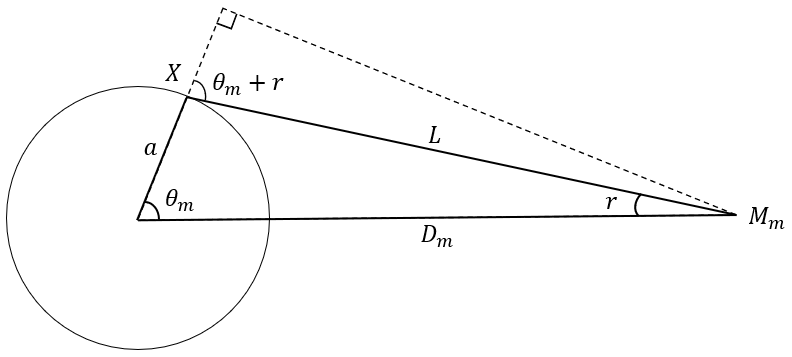
Figure 1 Schematic of the tidal forces generated by the moon, where M_m, a, D_m, and L are the moon, the radius of the earth, the distance to the moon, and the distance of the moon from any point X on the earth, respectively. θ_m is the zenith angle of point X relative to the moon, and r is the angle between the moon pointing to the center of the earth and point X.

According to analytic geometry and the law of cosines, we can obtain

$$\begin{array}{}\text{(2)}& {\displaystyle }& {\displaystyle }\sin \left({\mathit{\theta }}_{\mathrm{m}}+r\right)={\displaystyle \frac{D_{\mathrm{m}}\sin {\mathit{\theta }}_{\mathrm{m}}}{L}}\text{(3)}& {\displaystyle }& {\displaystyle }{L}^{\mathrm{2}}=D_{\mathrm{m}}^{\mathrm{2}}+a^{\mathrm{2}}-\mathrm{2}a{D}_{\mathrm{m}}\cos {\mathit{\theta }}_{\mathrm{m}},\end{array}$$

where D_m is the earth–moon distance. Based on these first three equations, Eq. (1) can be written as (see Supplement)

$$\begin{array}{}\text{(4)}& F_{\mathrm{tide},\mathrm{m}}\approx {\displaystyle \frac{\mathrm{3}}{\mathrm{2}}}{\displaystyle \frac{M_{\mathrm{m}}}{E}}{\left({\displaystyle \frac{a}{D_{\mathrm{m}}}}\right)}^{\mathrm{3}}g\sin \mathrm{2}{\mathit{\theta }}_{\mathrm{m}}.\end{array}$$

To compare with the traditional explicit tidal forcing formula of the eight most important constituents of the diurnal and semidiurnal tides, the instantaneous tidal height (tidal potential) caused by the moon due to equilibrium tides is diagnosed by the spatial integration of Eq. (4):

$$\begin{array}{}\text{(5)}& {\mathit{\eta }}_{\mathrm{tide},\mathrm{m}}=\underset{\mathrm{\Theta }}{\overset{{\mathit{\theta }}_{\mathrm{m}}}{\int }}\left(F_{\mathrm{tide},\mathrm{m}}\cdot a\right)\mathrm{d}{\mathit{\theta }}_{\mathrm{m}},\end{array}$$

where Θ is the zenith angle of the zero potential energy surface. With the global total tidal height at zero, ${\cos }^{\mathrm{2}}\mathrm{\Theta }=\mathrm{1}/\mathrm{3}$. Therefore, the instantaneous tidal height is

$$\begin{array}{}\text{(6)}& {\displaystyle }{\mathit{\eta }}_{\mathrm{tide},\mathrm{m}}={\displaystyle \frac{M_{\mathrm{m}}}{E}}{\displaystyle \frac{a^{\mathrm{4}}}{D_{\mathrm{m}}^{\mathrm{3}}}}{\displaystyle \frac{h}{\mathrm{2}}}\left(\mathrm{3}{\cos }^{\mathrm{2}}{\mathit{\theta }}_{\mathrm{m}}-\mathrm{1}\right),\end{array}$$

where the Love number h is introduced to represent the reduction in tidal forcing caused by the deformation of the solid earth. It is usually set equal to 0.7 (Wahr and Sasao, 1981; Griffies et al., 2004), which is adopted here.

Therefore, the tidal potential after taking into account tidal forcing due to both the moon and sun is as follows:

$$\begin{array}{}\text{(7)}& \begin{array}{rl}{\mathit{\eta }}_{\mathrm{tide}}& ={\displaystyle \frac{M_{\mathrm{m}}}{E}}{\displaystyle \frac{a^{\mathrm{4}}}{D_{\mathrm{m}}^{\mathrm{3}}}}{\displaystyle \frac{h}{\mathrm{2}}}\left(\mathrm{3}{\cos }^{\mathrm{2}}{\mathit{\theta }}_{\mathrm{m}}-\mathrm{1}\right)\\ & +{\displaystyle \frac{M_{\mathrm{s}}}{E}}{\displaystyle \frac{a^{\mathrm{4}}}{D_{\mathrm{s}}^{\mathrm{3}}}}{\displaystyle \frac{h}{\mathrm{2}}}\left(\mathrm{3}{\cos }^{\mathrm{2}}{\mathit{\theta }}_{\mathrm{s}}-\mathrm{1}\right).\end{array}\end{array}$$

The zenith angle θ_m is calculated as follows:

$$\begin{array}{}\text{(8)}& \cos {\mathit{\theta }}_{\mathrm{m}}=\sin \mathit{\phi }\sin {\mathit{\phi }}_{\mathrm{m}}+\cos \mathit{\phi }\cos {\mathit{\phi }}_{\mathrm{m}}\cos \left({\mathit{\lambda }}_{\mathrm{m}}-\mathit{\lambda }\right),\end{array}$$

where φ and λ are the latitude and longitude of the position X on the earth, respectively; φ_m and λ_m are the latitude and longitude of the projection point of the moon on the earth, respectively, and are both functions of universal time (Montenbruck and Gill, 2000). The zenith angle θ_s is similarly calculated.

Finally, explicit tidal forcing is introduced into the equation of barotropic mode motion:

$$\begin{array}{}\text{(9)}& \begin{array}{rl}{\displaystyle \frac{\partial \mathit{V}}{\partial t}}& =-{\displaystyle \frac{\mathrm{1}}{{\mathit{\rho }}_{\mathrm{0}}}}{\mathrm{\nabla }}_h{p}_{\mathrm{as}}-g^{\prime }{\mathrm{\nabla }}_h\left(\mathit{\alpha }\mathit{\eta }-{\mathit{\eta }}_{\mathrm{tide}}\right)\\ & +\stackrel{\mathrm{‾}}{P}+f\mathit{k}\times \mathit{V}+{\mathit{\tau }}_{\mathrm{tide}},\end{array}\end{array}$$

where V is the barotropic velocity, ${\mathrm{\nabla }}_h=\left(\partial /\partial x,\partial /\partial y\right)$; p_as is the sea surface air pressure; $g^{\prime }=g\mathit{\rho }/{\mathit{\rho }}_{\mathrm{0}}$ and α=0.948 represent the self-attraction of the earth and the correction generated by full self-attraction and loading (SAL) (Hendershott, 1972), which refers to the redistribution of the sea surface height between the earth and the ocean due to the existence of tide-generating potential. SAL treatment is a scalar approximation in order to make the calculation feasible. Currently, many tidal studies have applied SAL treatment (Simmons et al., 2004; Schiller and Fiedler, 2007; Griffies and Adcroft, 2008; Arbic et al., 2010). η is the sea surface fluctuation and η_tide is the instantaneous sea surface height due to equilibrium tides. $\stackrel{\mathrm{‾}}{P}$ represents the force from the vertically integrated baroclinicity in the ocean columns, and the last term on the right side of Eq. (10) is the vertically integrated Coriolis force. Introduction of tidal forcing leads to disruption of the dynamical balance of the ocean circulation in the original OGCM (Sakamoto et al., 2013), and Arbic et al. (2010) pointed out that the global tidal simulations must include parameterized topographic wave drag in order to accurately simulate the tides; we added a drag term τ_tide, in the barotropic equation, including parameterized internal wave drag due to the oscillating flow over the topography and the wave drag term due to the undulation of the sea surface (Jayne and Laurent, 2001; Simmons et al., 2004; Schiller and Fiedler, 2007).

3 Model description, numerical experimental design, and data

3.1 Model

The OGCM in this study is the second revised version of the LASG/IAP (State Key Laboratory of Numerical Modeling for Atmospheric Sciences and Geophysical Fluid Dynamics/Institute of Atmospheric Physics) climate system ocean model (LICOM2.0) (Liu et al., 2012; Dong et al., 2021), which adopts the free-surface scheme in η-coordinate models and offers the opportunity to explicitly resolve tides. The model domain is located between 78.5^∘ S and 87.5^∘ N with a 1^∘ zonal resolution. The meridional resolution is refined to 0.5^∘ between 10^∘ S and 10^∘ N and is increased gradually from 0.5 to 1^∘ between 10 and 20^∘. There are 30 levels in the vertical direction with 10 m per layer in the upper 150 m. Based on the original version of LICOM2.0, key modifications have been made: (1) a new sea surface salinity boundary condition was introduced that is based on the physical process of air–sea flux exchange at the actual sea–air interface (Jin et al., 2017); (2) intra-daily air–sea interactions are resolved by coupling the atmospheric and oceanic model components once every 2 h; and (3) a new formulation of the turbulent air–sea fluxes (Fairall et al., 2003) was introduced. The model has been used as the ocean component model of the Chinese Academy of Sciences Earth System Model (CAS-ESM 2.0) in its CMIP6 simulations (Zhang et al., 2020; Dong et al., 2021; Jin et al., 2021).

3.2 Numerical experimental design

To investigate the effect of tidal processes on the simulation of the ocean climate, three sets of experiments were conducted in the present study. The control experiment used the default LICOM2.0 without tidal forcing (denoted “CTRL” hereafter), Exp1 used the traditional explicit tidal forcing formula of the eight most important constituents of the diurnal and semidiurnal tides proposed by Griffies et al. (2009), and Exp2 used the new tidal forcing scheme.

For the control experiment, the Coordinated Ocean-ice Reference Experiments-I (CORE I) protocol proposed by Griffies et al. (2009) was employed, and the repeating annual cycle of climate atmospheric forcing from Large and Yeager (2004) was used. The model was first spun up for 300 years in order to reach a quasi-equilibrium state. All three experiments started from the quasi-equilibrium state (300th year) of the spin-up experiment and are integrated for 50 years under the same CORE I forcing fields. The diapycnal mixing of the Laurent et al. (2002) and Simmons et al. (2004) schemes was also applied to the baroclinic momentum and tracer equations. The hourly output of sea surface height in the last 10 years of the two tidal experiments was used to conduct the harmonic analysis and obtain the spatial information of tidal constituents.

3.3 Data

TPXO9v2 represent the assimilated data from a hydrodynamic model of the barotropic tides constrained by a satellite altimetry (Egbert and Erofeeva, 2002). To verify the effect of the two tidal schemes for high tidal amplitude regions, we also used two tidal stations, Yakutat (59.54^∘ N, 139.73^∘ W) and the Diego Ramirez Islands (56.56^∘ S, 68.67^∘ W), where the spectrum analysis was carried out. The station observations are from the sea level Data Assembly Center (DAC) of the World Ocean Circulation Experiment (WOCE) (Ponchaut et al., 2001). The data obtained from the Archiving, Validation and Interpretation of Satellite Oceanographic data (AVISO) (Schneider et al., 2013) are used in the observation of the dynamic sea level (DSL).

4 Results

4.1 Tidal forcing

Tides include spring tides, which are on the same line with the sun, the earth, and the moon, and neap tides, which are when the sun, the earth, and the moon are not aligned. Figures 2 and 3 show the spatial distributions of spring and neap tidal height η_tide calculated by the two tidal schemes. As expected, the two types of tides in Exp1 and Exp2 both have significant diurnal variations and exhibit a phase shift from east to west (Fig. 2). Both experiments simulated similar positions of the positive centers for spring tides, which are consistent with the overlap of the projected positions of the moon and the sun. It is important to note that the negative regions of the spring tide simulated in Exp2 exhibit large non-closed circular bands, which represents the elliptic model of the equilibrium tide theory (Schwiderski, 1980), and this is absent in Exp1 where the traditional explicit eight tidal constituents scheme is used.

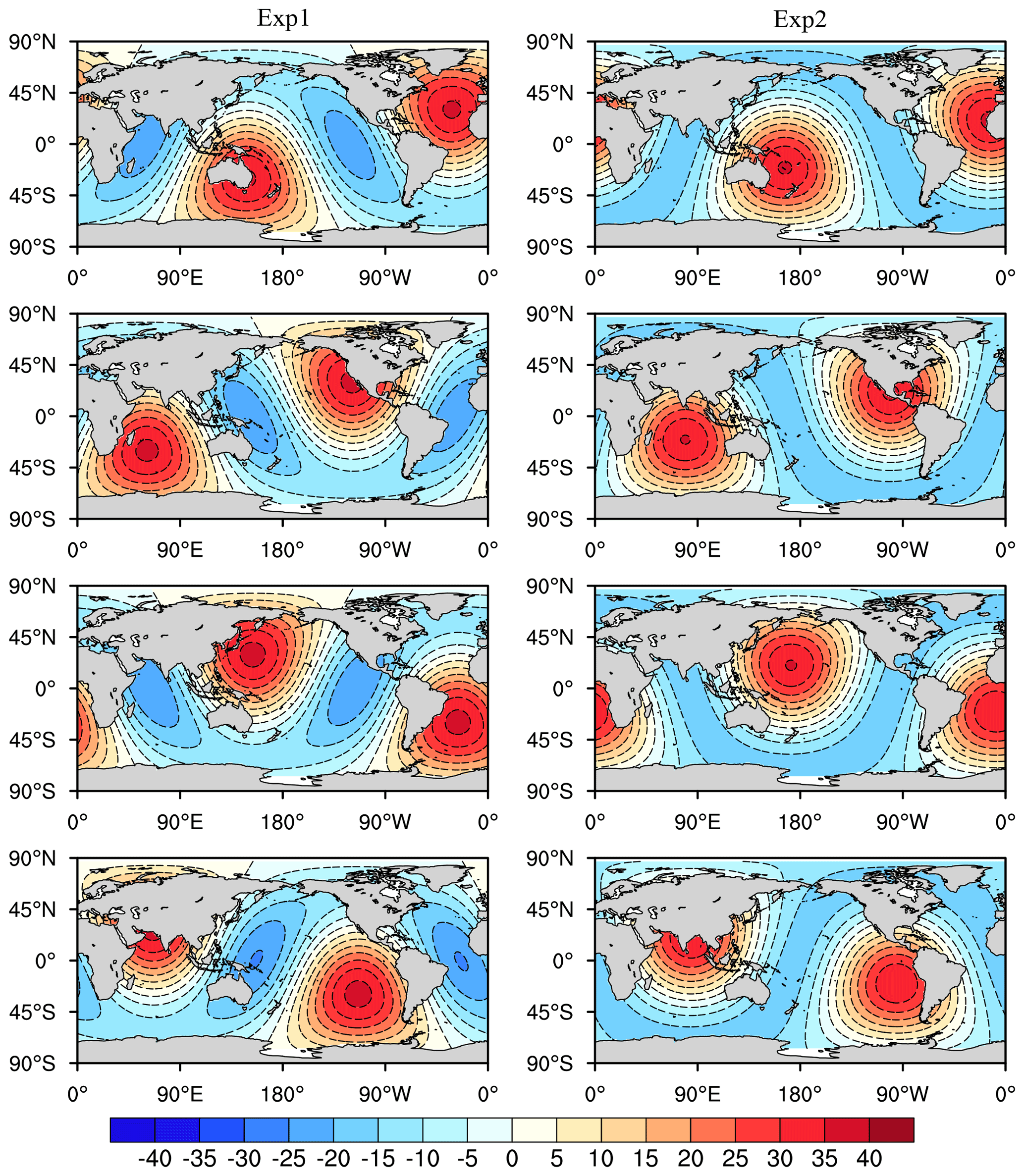
Figure 2 Spatial patterns of the spring tides for Exp1 (first column) and Exp2 (second column); the interval between the rows is 6 h. The units are centimeters.

There are pronounced differences in neap tides between Exp1 and Exp2 (Fig. 3). The neap tide simulated in Exp2 shows a larger meridional variation; the positive regions are mainly concentrated in the middle and low latitudes, and the negative regions are mainly concentrated in the high latitudes of the two hemispheres, because the projection positions of the sun and moon are located in the middle and low latitudes, resulting in the relatively weaker tidal potential in the high latitudes farther away from the projection position, which is consistent with the results of Gill (2015). However, Exp1 presents a larger zonal variation (positive–negative–positive–negative pattern), and the negative regions are concentrated in the middle and low latitudes rather than in the high latitudes; furthermore, the tidal potential in the polar regions is even higher than the negative regions in low latitudes, which means that the projection position of the sun is incorrect, locating at high latitudes rather than at low latitudes. Therefore, the new tidal scheme can represent the position of the sun better than the traditional scheme.

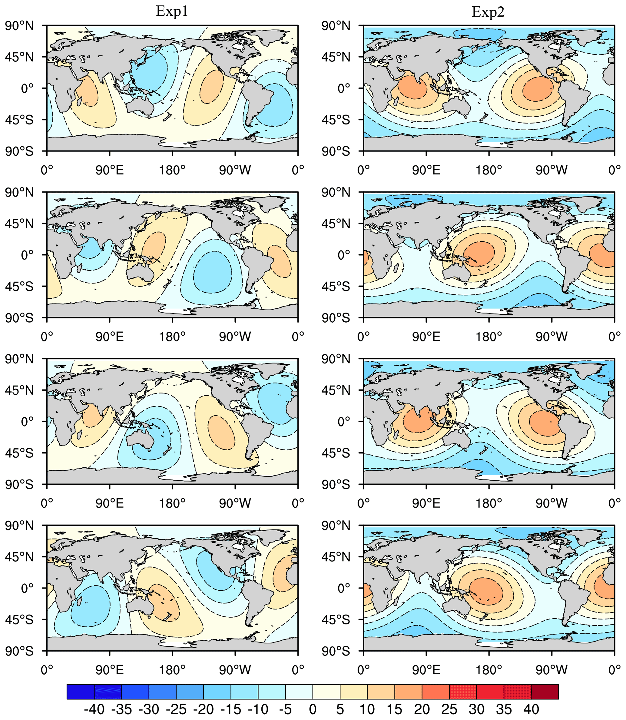
Figure 3 Spatial patterns of the neap tides for Exp1 (first column) and Exp2 (second column); the interval between the rows is 6 h. The units are centimeters.

4.2 Tidal constituents

The harmonic analysis of the hourly sea surface height data simulated by the two tidal schemes is carried out in order to obtain the amplitude and phase of each major tidal constituent. TPXO9v2 is used as the observed data (Egbert and Erofeeva, 2002). In this study, we mainly focus on the amplitudes and phases of the two largest constituents among the eight tidal constituents, including a full diurnal constituent of K1 and a half-diurnal constituent of M2. To quantitatively compare the simulations of tidal constituents by the two schemes, we calculated the mean square error following Shriver et al. (2012):

$$\begin{array}{}\text{(10)}& \begin{array}{rl}{\text{total error}}^{\mathrm{2}}& =\left[{\displaystyle \frac{\mathrm{1}}{\mathrm{2}}}{\left(A_{\mathrm{model}}-A_{\mathrm{TPXO}}\right)}^{\mathrm{2}}\right]\\ & +\left[A_{\mathrm{model}}{A}_{\mathrm{TPXO}}\right.\\ & \left.\left(\mathrm{1}-\cos \left({\mathit{\varphi }}_{\mathrm{model}}-{\mathit{\varphi }}_{\mathrm{TPXO}}\right)\right)\right],\end{array}\end{array}$$

where A_model and A_TPXO are simulated and observed amplitudes, respectively, and ϕ_model and ϕ_TPXO are simulated and observed phases, respectively. The total error in each tidal constituent can be divided into amplitude error and amplitude-weighted phase error (phase error); the former is the first term on the right side of Eq. (11), and the latter is the second term on the right side of Eq. (11).

Figure 4 shows the respective amplitudes and phases of K1 for the observation, Exp1, and Exp2, the total errors for the two experiments against the observation, and the difference in the total errors between the two experiments. The amplitudes and phases of K1 simulated in both Exp1 and Exp2 are similar to the observation (Fig. 4a–c). The large values of the amplitudes of K1 are located in the North Pacific Ocean, Indonesia, Ross Sea, and Weddell Sea. However, Exp1 simulated a larger amplitude of K1, and the extent of the large amplitude is too excessive, especially for the North Pacific Ocean and Southern Ocean, compared to the extent of the large amplitude in the observation and Exp2, which is consistent with the results of Yu et al. (2016). The simulated amplitude of K1 by Exp2 is significantly improved and closer to the observation. The global mean values of K1 are 11.58, 14.74, and 10.50 cm for the observation, Exp1, and Exp2, respectively.

Figure 4 Spatial patterns of the amplitude and phase of K1 for (a) the observation (Obs), (b) Exp1, (c) Exp2, (d) the total error for Exp1, (e) the total error for Exp2, and (f) the difference in error between Exp2 and Exp1. The observation is from TPXO9v2 (Egbert and Erofeeva, 2002). The units are centimeters, and the lines of the constant phase are plotted every 45^∘ in black.

The total error patterns of K1 in Exp1 and Exp2 show similar distributions (Fig. 4d and e); large values are located in the Southern Ocean and the North Pacific. The total error of K1 in Exp2 is smaller than in Exp1 in most regions except for the Arabian Sea, especially for the Southern Ocean, the North Pacific, and the eastern equatorial Pacific (Fig. 4f). The global mean total errors of K1 in Exp1 and Exp2 are 7.43 and 6.28 cm, respectively. According to Eq. (11), the total error of K1 is divided into amplitude error and phase error (Fig. 5). Compared with Exp1, the amplitude error of K1 is significantly improved in most regions, especially for the large amplitude of K1 regions, which is the main reason for the smaller total error of K1 in Exp2, although the phase error is also slightly reduced; this suggests that the new tidal scheme leads to a better simulation of the amplitude and phase of K1, especially for the amplitude simulation. The global mean of the amplitude errors in Exp1 and Exp2 are 4.97 and 3.73 cm, respectively, and the corresponding phase errors in both experiments are 5.52 and 5.06 cm, respectively.

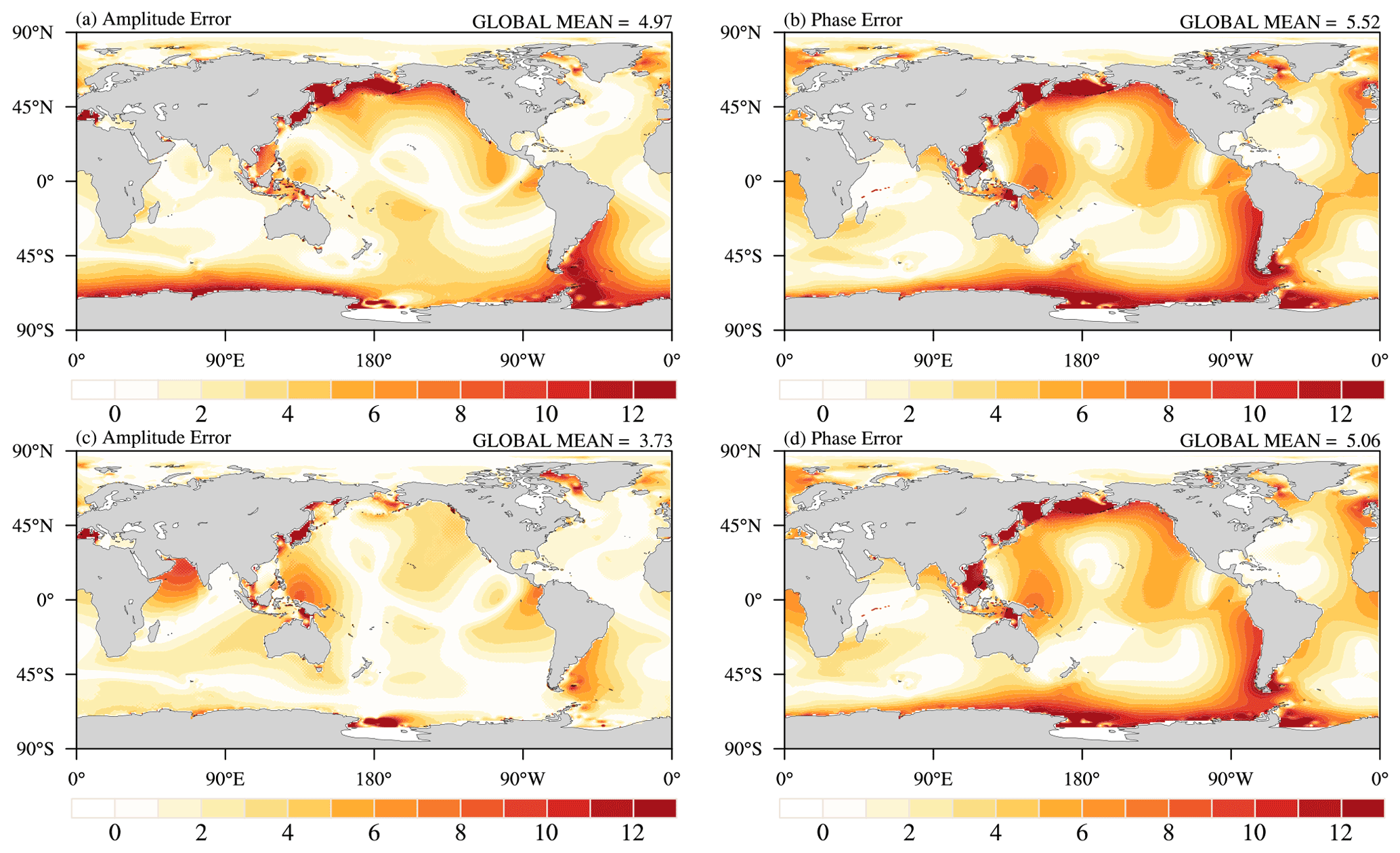
Figure 5 The contributions to the total error of K1 resulting from errors in (a) tidal amplitude and (b) phase for Exp1; (c) and (d) are the same, but for Exp2. The units are centimeters.

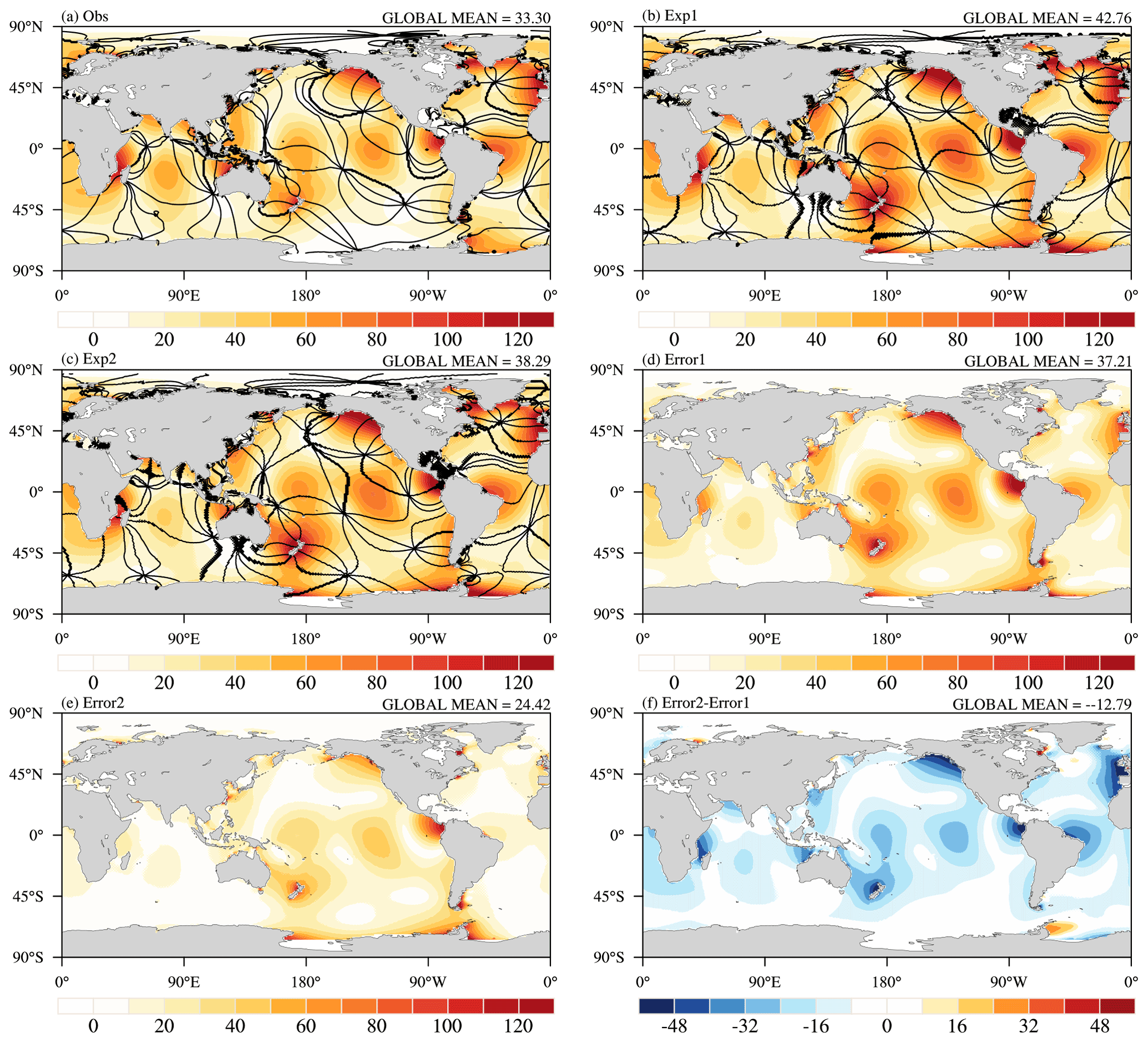
Figure 6 Spatial patterns of the amplitude and phase of M2 for (a) the observation (Obs), (b) Exp1, (c) Exp2, (d) the total error for Exp1, (e) the total error for Exp2, and (f) the difference in error between Exp2 and Exp1. The observation is from TPXO9v2 (Egbert and Erofeeva, 2002). The units are centimeters, and the lines of the constant phase are plotted every 45^∘ in black.

M2 is known to be the largest tidal constituent (Griffies et al., 2009). Figure 6 shows the respective amplitudes and phases of M2 for the observation, Exp1, and Exp2, as well as the total errors for the two experiments against the observation and the difference in the total errors between the two experiments. Both Exp1 and Exp2 can reasonably simulate the overall spatial distribution patterns of M2 amplitude and phase (Fig. 6a–c). The maximum values of the amplitude are located in the Bay of Alaska, the eastern equatorial Pacific, Tasman Sea, and the North Atlantic. The amplitudes of M2 simulated in both Exp1 and Exp2 are larger than the observation, especially for the Ross Sea and Weddell Sea, although Exp2 exhibits some alleviation of the bias when compared with Exp1. The global mean values of M2 are 33.30, 42.76, and 38.29 cm for the observation, Exp1, and Exp2, respectively.

The total error patterns of M2 in Exp1 and Exp2 also show similar features (Fig. 6d and e); the large values are located in the large amplitude of M2 regions, noting the smaller magnitude of the total error of M2 in Exp2 relative to Exp1 in most regions. The global mean of total error in Exp2 (24.42 cm) is obviously lower than in Exp1 (37.21 cm). In addition, the amplitude error and the phase error of M2 in Exp2 are both improved, the global mean of amplitude errors in Exp1 and Exp2 are 14.77 and 12.86 cm, respectively, and the corresponding phase errors in Exp1 and Exp2 are 34.16 and 20.76 cm, respectively. Inconsistent with K1, the smaller total error of M2 in Exp2 relative to Exp1 is mainly the result of the phase error; in particular, the phase errors of Exp2 are almost eliminated in the Indian Ocean and the Atlantic Ocean (Fig. 7). This indicates the new tidal scheme results in a better simulation of M2, especially for the phase simulation. Compared with Exp1, the total errors of K1 and M2 in Exp2 are reduced by 21.85 % and 32.13 % respectively.

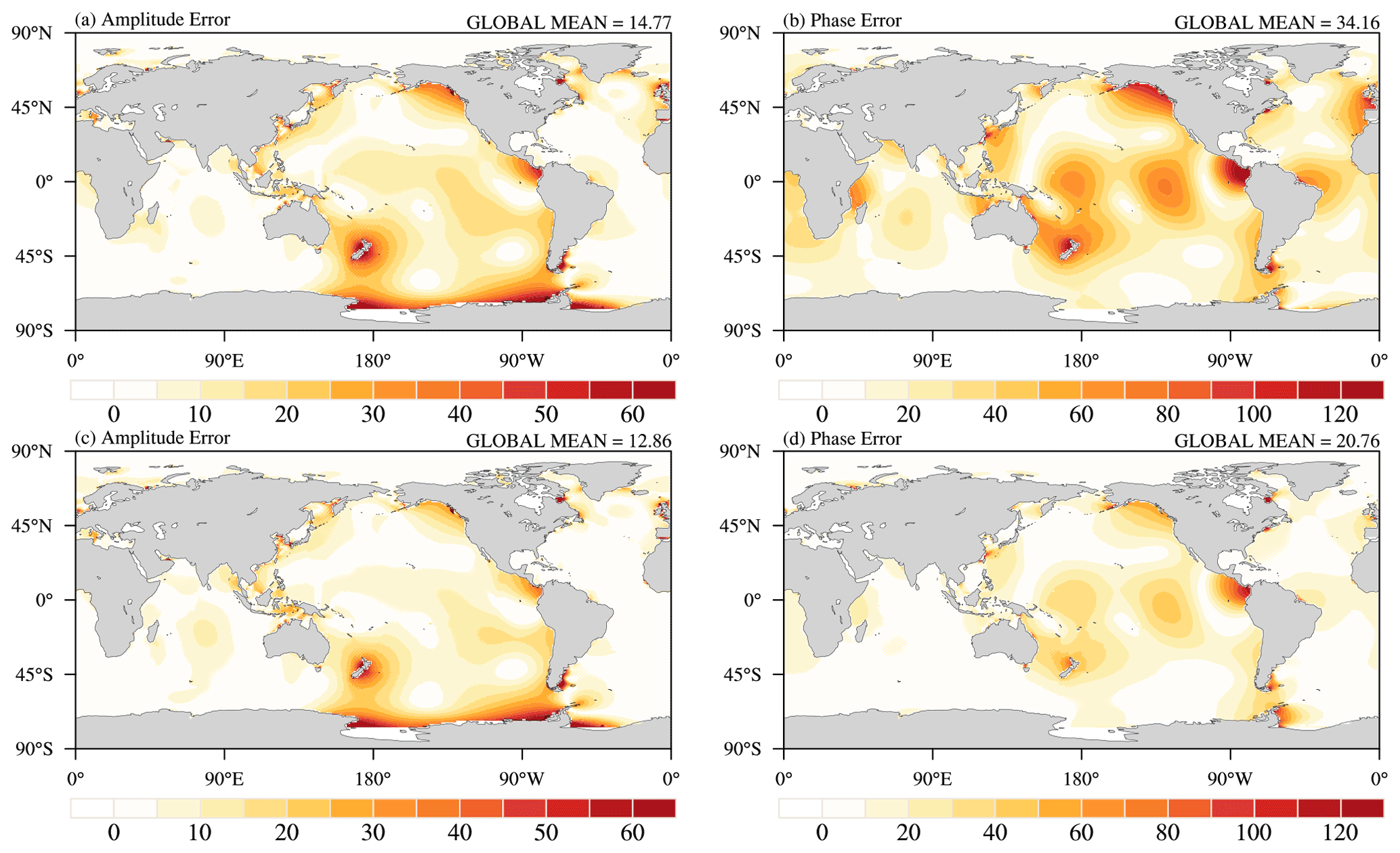
Figure 7 The contributions to the total error of M2 resulting from errors in (a) tidal amplitude and (b) phase for Exp1; (c) and (d) are the same, but for Exp2. The units are centimeters.

Furthermore, we also investigate the amplitudes and total errors of the remaining six tidal constituents (O1, P1, Q1, S2, N2, and K2) simulated using two schemes. For amplitudes, the global means of the three constituents (O1, P1, and K2) in Exp2 are closer to the observed values relative to Exp1. The global mean observed values for the O1, P1, Q1, S2, N2, and K2 constituents are 8.34, 3.62, 1.76, 13.35, 7.08, and 3.75 cm, respectively, and the corresponding values in Exp1 (Exp2) are 10.59 cm (9.79 cm), 13.49 cm (9.47 cm), 1.62 cm (2.19 cm), 12.45 cm (9.85 cm), 7.74 cm (9.79 cm), and 10.89 cm (7.33 cm), respectively (Table 1). The global mean total errors for the remaining six constituents in Exp2 (with the exception of Q1 and N2) are smaller than those in Exp1, and the global mean total errors of the remaining six constituents in Exp1 (Exp2) are 8.89 cm (5.34 cm), 9.53 cm (6.26 cm), 1.29 cm (1.47 cm), 11.26 cm (9.40 cm), 5.84 cm (6.76 cm), and 10.32 cm (6.55 cm), respectively. Compared with Exp1, the improved total errors of O1 and S2 in Exp2 are mainly the result of the smaller phase errors, and the improvement of the total error of P1 in Exp2 is predominantly due to the lower amplitude error. The global mean amplitude errors of O1, P1, S2, and K2 in Exp1 (Exp2) are 3.28 cm (3.16 cm), 9.18 cm (5.58 cm), 5.11 cm (5.68 cm), and 6.50 cm (3.72 cm), respectively, and the corresponding phase errors are 8.26 cm (4.30 cm), 2.57 cm (2.84 cm), 10.04 cm (7.49 cm), and 8.01 cm (5.39 cm), respectively (Table 1). These results indicate that the new formulation of the tidal scheme can better simulate more constituents of tides relative to the traditional method of eight tidal constituents with empirical amplitudes and frequencies.

Table 1 Global mean values of the amplitudes of the eight tidal constituents during observation, Exp1, and Exp2, and the amplitude, phase, and total errors of the eight tidal constituents in Exp1 and Exp2. The units are centimeters. The better amplitude and lower errors in Exp2 relative to Exp1 are marked in bold.

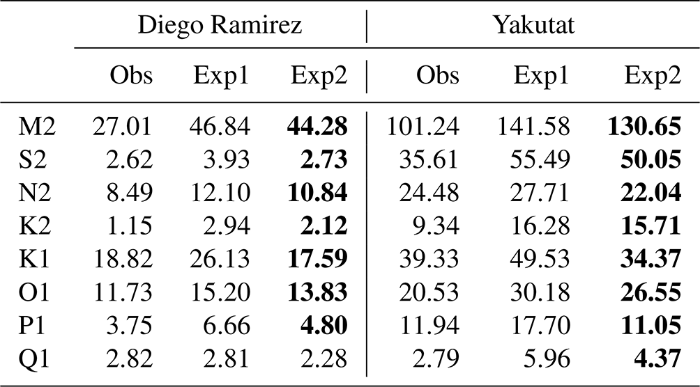
To further evaluate the simulation of the eight tidal constituents by using the two tidal schemes, we also made a spectrum analysis at the Diego Ramirez Islands (56.56^∘ S, 68.67^∘ W) and Yakutat (59.54^∘ N, 139.73^∘ W) tidal stations, which are located in regions with large tidal amplitudes (Fig. 8). Both Exp1 and Exp2 can reasonably reproduce the amplitudes and frequencies of the eight main tidal constituents at the Diego Ramirez Islands and Yakutat stations, although most of the simulated amplitudes in Exp1 are much larger than the observed data. The larger amplitude biases of the eight main tidal constituents at both stations (except for the Q1 constituent at the Diego Ramirez station) are all significantly improved in Exp2 (Table 2). For instance, the amplitude of M2 in Exp1 at the Yakutat station is 141.58 cm, and it is reduced to 130.65 cm in Exp2, which is closer to the observed data (101.24 cm). The amplitude of K1 in Exp1 at the Diego Ramirez station is 26.13 cm, and it is reduced to 17.59 cm in Exp2, which is closer to the observed data (18.82 cm). On the basis of these preliminary evaluations, compared to the traditional explicit eight tidal constituents scheme, the new tidal scheme can better reproduce the spatial patterns of the amplitude of tidal constituents and tidal forcing, especially for the magnitude of the amplitude. Furthermore, we conducted two experiments (one using the traditional tidal scheme, the other applying the new tidal scheme) by also adopting the practical scheme following Sakamoto et al. (2013), and we found that the errors (including the phase error and total error) of all eight tidal constituents of the experiment using the new tidal scheme are fewer than when applying the tradition tidal scheme (Table S1 in the Supplement).

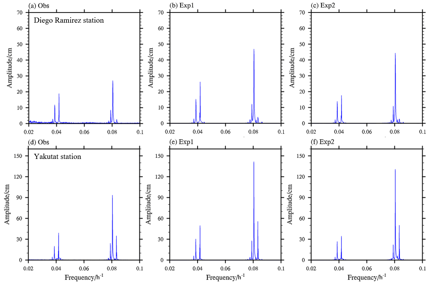
Figure 8 Spectrum analysis of sea surface height for (a, d) the observation (Obs), (b, e) Exp1, and (c, f) Exp2. The observation is from WOCE (Ponchaut et al., 2001). The upper panels are for the Diego Ramirez Islands (56.56^∘ S, 68.67^∘ W) and the lower panels are for Yakutat (59.54^∘ N, 139.73^∘ W).

Table 2 The amplitudes of the eight tidal constituents during the observation (Obs), Exp1, and Exp2 at the Diego Ramirez Islands (56.56^∘ S, 68.67^∘ W) and Yakutat (59.54^∘ N, 139.73^∘ W). The observation is from WOCE (Ponchaut et al., 2001); the units are centimeters. The better amplitude in Exp2 relative to Exp1 is marked in bold.

4.3 Dynamic sea level (DSL)

Figure 9 shows the spatial distributions of DSL that is defined as the sea level associated with the fluid dynamic state of the ocean (Griffies and Greatbatch, 2012; Griffies et al., 2016) for the observation, CTRL, and the bias in CTRL, Exp1, and Exp2 relative to the observations as well as the difference between Exp2 and Exp1. The observation is obtained from the Archiving, Validation and Interpretation of Satellite Oceanographic data (AVISO) (Schneider et al., 2013). The DSL simulated by CTRL shows a low DSL located in the Labrador Sea, the Nordic Seas, and the Southern Ocean, and a high DSL in the tropical and subtropical Pacific and Indian Oceans (Fig. 9b), which is consistent with the observed data (Fig. 9a). Therefore, the ocean model, LICOM2.0, without a tidal process can reproduce the basic pattern of DSL, but large biases also exist (Fig. 9c); there is a dipole pattern bias located across the Antarctic Circumpolar Circulation (negative bias to the north and positive bias to the south), a striking negative bias in the North Atlantic, and a slightly positive bias in the western equatorial Pacific.

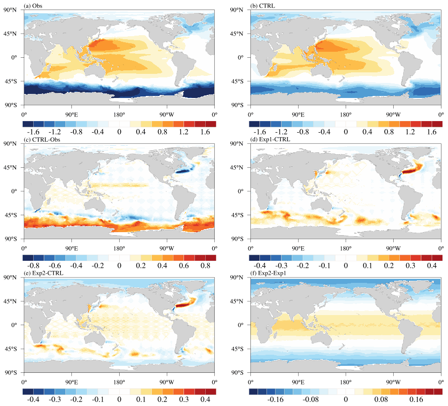
Figure 9 Spatial patterns of the dynamic sea level for (a) the observation (Obs), (b) CTRL, (c) the difference between CTRL and observation, (d) the difference between Exp1 and CTRL, (e) the difference between Exp2 and CTRL, and (f) the difference between Exp2 and Exp1. The observation is from AVISO (Schneider et al., 2013); the units are meters.

The DSLs in both Exp1 and Exp2 are improved and the striking negative bias for the North Atlantic is reduced (Fig. 9d and e), which can be attributed to the improvement of the path of the North Atlantic Gulf Stream due to the effects of tides, as pointed out by Müller et al. (2010). There are some significant differences between Exp1 and Exp2. Compared to Exp1, Exp2 exhibits a striking latitudinal distribution feature (Fig. 9f), which shows a decreasing spatial pattern from the Equator to the poles, with positive values in the tropic region and a negative pattern in high latitudes. This is because Exp2, in applying the new formulation of the tidal scheme, can consider the positions of both the sun and moon relative to Exp1. Compared with Exp1, the positive bias in the Southern Ocean simulated by CTRL is improved in Exp2, as exhibited by the negative difference between Exp2 and Exp1 at high latitudes. This is because Exp2, applying the new formulation of the tidal scheme, can reasonably consider the positions of both the sun and moon relative to Exp1, which makes the DSL higher in low latitude compared with that in high latitude due to the effect of gravity.

5 Summary

In this paper, a new explicit tidal scheme is introduced to a global ocean model. The scheme uses the positional characteristics of the moon and the sun to calculate the tides directly instead of applying empirical specifications, such as the amplitudes and frequencies of tides, which were used in traditional methods. The new tidal scheme has some unique advantages: It can accurately provide instantaneous tidal potentials, since both astronomers and oceanographers have well established models for determining the exact position of the sun and the moon by Julian and for calculating the instantaneous tidal potential by their projected positions. The traditional tidal scheme does not guarantee the correct transient tidal potential at any given time, as described in Sect. 4.1. The traditional method does not cover all tidal constituents, and thus it is more suitable for studying only one specific tidal constituent rather than the full real tidal process in the OGCM. Besides, in the traditional scheme, the tidal potential is introduced in the form of sine wave, so that the climate state of tidal potential is zero at any position. The new tidal method does not impose this particular time variation.

Compared with the traditional explicit scheme with eight tidal constituents, we found that the new tidal scheme can better simulate the spatial characteristics of spring and neap tides. It significantly reduces the biases of larger amplitudes in the traditional explicit tidal scheme, and reproduces the spatial patterns of tidal constituents better than the traditional method. In theory, this scheme is also better suited than the traditional method to simulate sea level height at regional scales which may not all be captured by the small number of prescribed constituents.

Furthermore, the total errors of the eight tidal constituents are studied, including amplitude errors and phase errors. The total errors of the eight tidal constituents simulated by the new tidal scheme, with the exception of N2 and Q1, are all smaller than those simulated by the traditional method. Compared with the traditional method, the improved total errors of M2, O1, and S2 simulated by the new tidal scheme are mainly the result of the better phase simulation (the smaller phase errors); the reduction in the total errors of K1 and P1 is predominantly due to the improvement in the amplitude simulation (with fewer amplitude errors); and the smaller total error of K2 is associated with both the improvements in the amplitude and phase simulation (both the smaller phase and amplitude errors).

The influence of tidal forcing on the simulation of DSL is also investigated. We found both tidal schemes can significantly improve the simulation of DSL, and the striking negative bias for the North Atlantic in CTRL is reduced. Compared with the traditional explicit scheme of eight tidal constituents, the new tidal scheme exhibits a latitudinal variation of DSL with a positive difference in the tropics and a negative pattern in high latitudes, which improves the significant positive bias of the Southern Ocean in CTRL.

It should be noted that the wave drag term formula proposed by Schiller and Fiedler (2007) and the drag from internal wave generation (Jayne and Laurent, 2001; Simmons et al., 2004) are adopted in the present study to decay the tidal energy, which is likely too strong in both tidal experiments, especially with the traditional tidal forcing formula. Implementing a more appropriate tidal drag parameterization in an OGCM still needs to be carried out. In addition, the explicit introduction of tides into an OGCM is only one step toward upgrading ocean modeling. A more detailed investigation into the impacts of the new tidal scheme on simulated ocean circulations will be our future work, especially in an OCGM with a finer resolution and in a fully coupled mode.