the Creative Commons Attribution 4.0 License.
the Creative Commons Attribution 4.0 License.
 | 01 Jun 2022
Assessing the roles emission sources and atmospheric processes play in simulating δ15N of atmospheric NOx and NO3− using CMAQ (version 5.2.1) and SMOKE (version 4.6)
Greg Michalski
Nitrogen oxides (NOx= nitric oxide (NO) + nitrogen dioxide (NO2)) are important trace gases that affect atmospheric chemistry, air quality, and climate. Contemporary development of NOx emissions inventories is limited by the understanding of the roles of vegetation (net NOx source or net sink), vehicle emissions from gasoline- and diesel-powered vehicles, the application of NOx emission control technologies, and accurate verification techniques. The nitrogen stable isotope composition (δ15N) of NOx is an effective tool to evaluate the accuracy of the NOx emission inventories, which are based on different assumptions. In this study, we traced the changes in δ15N values of NOx along the “journey” of atmospheric NOx, driven by atmospheric processes after different sources emit NOx into the atmosphere. The 15N was incorporated into the emission input dataset, generated from the US EPA trace gas emission model SMOKE (Sparse Matrix Operator Kernel Emissions). Then the 15N-incorporated emission input dataset was used to run the CMAQ (Community Multiscale Air Quality) modeling system. By enhancing NOx deposition, we simulated the expected δ15N of NO, assuming no isotope fractionation during chemical conversion or deposition. The simulated spatiotemporal patterns in NOx isotopic composition for both SMOKE outputs (simulations under the “emission only” scenario) and CMAQ outputs (simulations under the “emission + transport + enhanced NOx loss” scenario) were compared with corresponding measurements in West Lafayette, Indiana, USA. The simulations under the emission + transport + enhanced NOx loss scenario were also compared to δ15N of NO at NADP (National Atmospheric Deposition Program) sites. The results indicate the potential underestimation of emissions from soil, livestock waste, off-road vehicles, and natural-gas power plants and the potential overestimation of emissions from on-road vehicles and coal-fired power plants, if only considering the difference in NOx isotopic composition for different emission sources. After considering the mixing, dispersion, transport, and deposition of NOx emission from different sources, the estimation of atmospheric δ15N(NOx) shows better agreement (by ∼ 3 ‰) with observations.
- Article
(5771 KB) - Full-text XML
-
Supplement
(7230 KB) - BibTeX
- EndNote


Nitrogen oxides (NOx= NO + NO2) are important trace gases that affect atmospheric chemistry, air quality, and climate. The main sources of tropospheric NOx are anthropogenic emissions from vehicles, power plants, agriculture, livestock waste, as well as natural emissions from lightning and the by-product of nitrification and denitrification occurring in soil (Galloway et al., 2004). The NOx photochemical cycle generates OH and HO2 radicals, organic peroxy radicals (RO2), and ozone (O3), which ultimately oxidize NOx into NOy (NOy = NOx+ HONO + HNO3+ HNO4+ N2O5+ other N oxides). During the photochemical processes that convert NOx to NOy, ground-level concentrations of O3 become elevated, and secondary particles are generated (Seinfeld and Pandis, 2006). Secondary aerosols are hazardous to human health (Lighty et al., 2000) and affect cloud physics, enhancing the reflection of solar radiation (Schwartz, 1996). Thus, the importance of NOx in air quality, climate, and human and environmental health makes understanding the spatial and temporal variation in the sources of NOx a vital scientific question.
Despite years of research, however, there are still several significant uncertainties in the NOx budget. About 15 %–40 % of global NOx emissions, ranging from 4 to 15 Tg N yr−1, is derived from global soil NOx emissions, yet evaluating and verifying emission rates using laboratory measurements, field measurements, and satellite observations is still a challenge (Jaegleì et al., 2005; Yan et al., 2005; Stehfest and Bouwman, 2006; Vinken et al., 2014; Rasool et al., 2016). Soil NOx emissions vary by different biome types, meteorological conditions, N fertilizer application, and soil physicochemical properties (Ludwig et al., 2001). Furthermore, the role of vegetation is to act as a net source of atmospheric NOx when ambient NOx concentration is below the “compensation point” versus acting as a net sink of atmospheric NOx when ambient NOx concentrations are above it (Johansson, 1987; Thoene et al., 1996; Slovik et al., 1996; Weber and Rennenberg, 1996). This significantly impacts the biotic NOx emission inventory (Almaraz et al., 2018). Uncertainties also exist in the amount of NOx emitted during the combustion of fossil fuels by vehicles and industry. According to Parrish (2006), the estimation of on-road vehicle NOx emission has at least 10 % to 15 % uncertainty. For the mileage-based algorithm, which is used in the National Emission Inventory (NEI), the uncertainty is caused by the limited number of sites to determine the emission factors of vehicle classifications and emission types (Ingalls, 1989; Pierson et al., 1990; Fujita et al., 1992; Pierson et al., 1996; Singer and Harley, 1996). The uncertainty in power plant NOx emissions results from the choice of emission control technologies, of which the removal efficiencies of NOx emission are different. NOx removal by low NOx burning, over-fire air reduction, and selective non-catalytic reduction is highly variable, ranging from 50 % to 75 % (Srivastava et al., 2005).
The nitrogen stable isotope composition (δ15N) of NOx might be a useful tool to help resolve the uncertainties of how NOx emission sources vary in space and time because NOx sources have distinctive 15N 14N ratios (Ammann et al., 1999; Felix et al., 2012; Felix and Elliott, 2013; Fibiger et al., 2014; Heaton, 1987; Hoering, 1957; Miller et al., 2017; Walters et al., 2015a, b, 2018). This variability in NOx 15N 14N ratios is quantified by
where 15NOx 14NOx is the measurement of 15N 14N in atmospheric NOx, compared with the ratios in air N2=0.0036 (for brevity, the δ15N value of any NOy compound will be denoted as δ15NOy, e.g., δ15NO). Previous research has shown that there are unique differences in δ15N values for NOx from different emission sources and significant variations within each source (Fig. 1). This uniqueness can potentially be used to partition the relative importance of various NOx sources in a mixed atmosphere. For example, Redling et al. (2013) found higher δ15N of NO2 in samples collected closer to the highway compared to those adjacent to a forest, showing the emissions from vehicles were dominant near the highway. A strong positive correlation between δ15NO and NOx emission from coal-fired power plants within 400 km radial area of study sites of deposition suggests local power plant NOx emissions impacted regional NOx budgets (Elliott et al., 2007, 2009). What is lacking is a systematic way of evaluating δ15NOy values in numerous studies in the context of NOx sources, regional emissions, meteorology, and atmospheric chemistry (Elliott et al., 2009; Garten, 1992; Hall et al., 2016; Occhipinti, 2008; Russell et al., 1998).
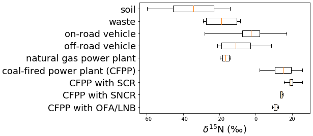
Figure 1Box (lower quartile, median, upper quartile) and whisker (lower extreme, upper extreme) plot of the distribution of δ15N values for various NOx emission sources.
Here we have simulated the emission of 15NOx and its mixing in the atmosphere and compared the predicted δ15N (NOx, NO) values to observations. The δ15NOx values are impacted by three main factors. The first is the inherent variability of the δ15NOx emissions in time and space. Secondly, atmospheric processes mix the emitted NOx, dispersing multiple emission sources within a mixing lifetime relative to the NOx chemical lifetime (2–7 h), which depends on its concentration and photooxidation chemistry, that also vary in time and by location (Laughner and Cohen, 2019). And thirdly, isotope effects occurring during tropospheric photochemistry may alter the δ15NOx emissions as they are transformed from NOx into NOy. In this paper, we consider the effects from the first and second considerations, the temporal and spatial variation in NOx emission, and the impacts from atmospheric transport and deposition processes (source and mixing hypothesis). We accomplish this by incorporating an input dataset of 15N emissions used in simulations by the CMAQ (Community Multiscale Air Quality) modeling system. In a previous paper we have discussed the impacts of tropospheric photochemistry by incorporating a 15N chemical mechanism (Fang et al., 2021) into CMAQ. The ultimate goal is to evaluate the accuracy of the NOx emission inventory using 15N.
2.1 Incorporating 15N into NOx emission datasets
The EPA trace pollutant emission model SMOKE (Sparse Matrix Operator Kernel Emissions) was used to simulate 14NOx and 15NOx emissions. 14NOx emissions were estimated using the SMOKE model based on the 2002 NEI (National Emission Inventory; United States Environmental Protection Agency, 2014), and 15N emissions were determined using these 14NOx emissions and the corresponding δ15N values of NOx sources from previous research (Table 1). Using the definition of δ15N (‰), 15NOx emitted by each SMOKE processing category (area, biogenic, mobile, and point) was calculated by
where 14NOx(i) denotes the NOx emissions for each category (i) obtained from NEI and SMOKE, and 15RNOxi is a 15N emission factor (15NOxi 14NOxi) calculated by rearranging Eq. (1):
where δ15NOx(i) is the δ15N value of some NOx source (i= area, biogenic, mobile, and point).
Annual NOx emissions for 2002 were obtained from the NEI at the county level and were converted into hourly emissions on a 12 km × 12 km grid as previously published (Spak et al., 2007). The modeling domain includes latitudes between 37 and 45∘ N and longitudes between 98∘ W and 78∘ W, which fully covers the Midwestern US (Fig. 2, in yellow). SMOKE categorizes NOx emissions into four “processing categories”: biogenic, mobile, point, and area (Table 1). The choice of the 2002 version of NEI is, in part, arbitrary. However, to compare the model-predicted δ15N values with observations, it requires the emission inventory to be relevant to the same timeframe as the δ15N measurements of the NOy. The datasets we compare to the model (discussed below) span from 2002 to 2009; thus the 2002 inventory is more relevant than later inventories (2014 onward). The county-level annual 14NOx emission for the Midwestern US from NEI was converted to the dataset with hourly 14NOx emissions.
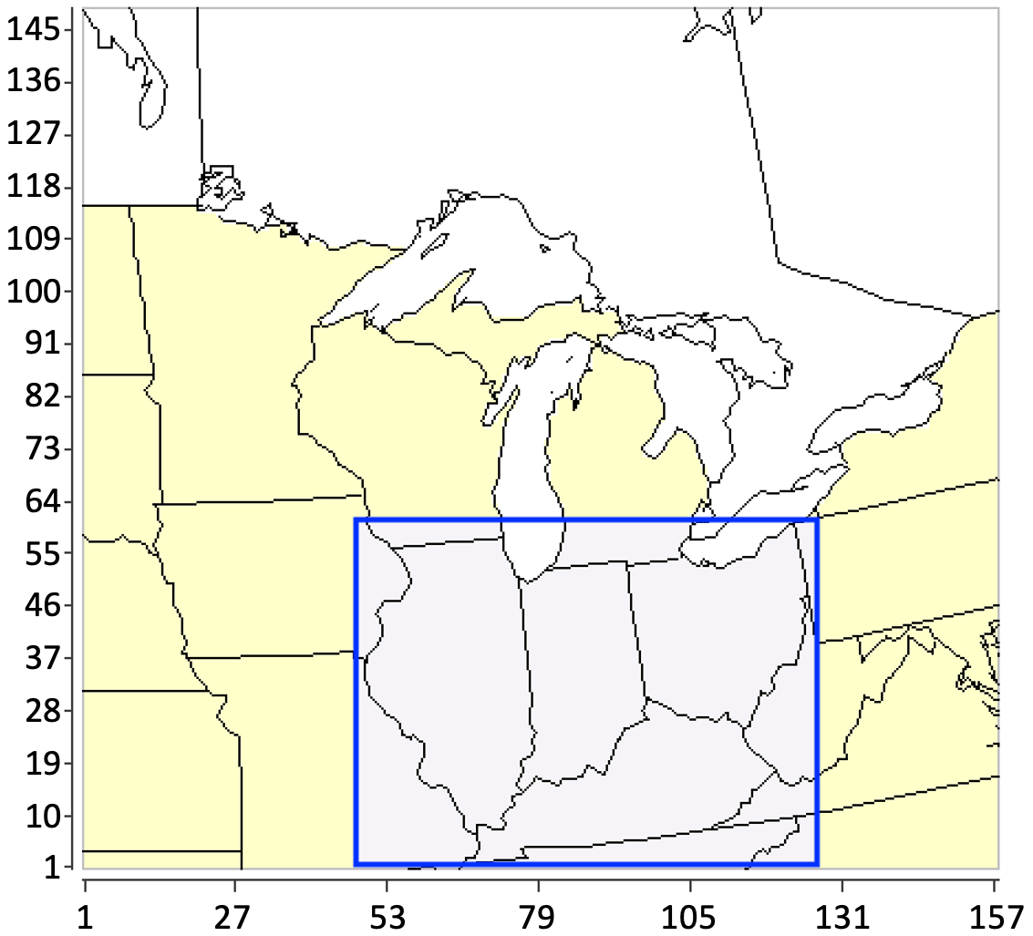
Figure 2The full geographic domain (yellow) and extracted domain (light grayish purple) for the study.
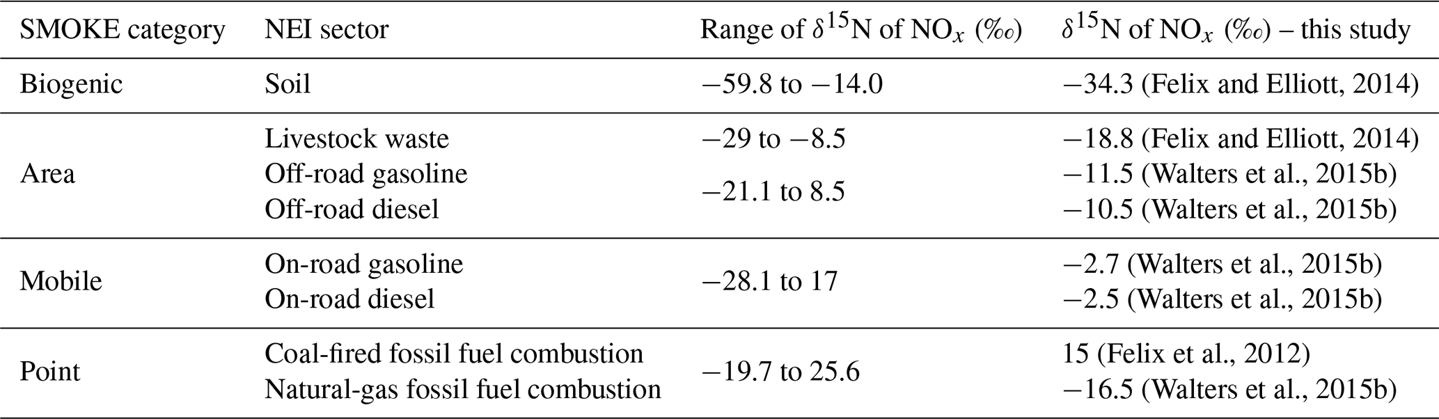
Table 1The δ15N values (in ‰) for NOx emission sources based on SMOKE processing category and NEI sector.
2.1.1 Biogenic 15NOx emissions
The NOx emission from the soil (biogenic) was modeled in SMOKE using standard techniques (details in the Supplement), and the δ15N values of biogenic NOx were taken from previous studies. Li and Wang (2008) measured the NO fluxes using dynamic flow chambers for 2 to 13 d after cropland soil was fertilized by either urea (n=9) or ammonium bicarbonate (n=9), and the δ15NOx ranged from −48.9 ‰ to −19.8 ‰. Felix and Elliott (2014) used passive samplers to collect NO2 in a cornfield for 20 d, with low (−30.8 ‰) and high (−26.5 ‰) fertilizer application. Using active samplers, Miller et al. (2018) collected NO2 between May and June, finding δ15N ranging from −44.2 ‰ to −14.0 ‰ (n=37); Yu and Elliott (2017) measured −59.8 ‰ to −23.4 ‰ in 15 samples from soil plots in a fallow field 2 weeks after the precipitation. Based on these studies, we adopted an average δ15N value for NOx emissions from the soil of −34.3 ‰ (Li and Wang, 2008; Felix and Elliott, 2014; Yu and Elliott, 2017; Miller et al., 2018).
2.1.2 Mobile 15NOx emissions
The SMOKE NOx emission from on-road vehicles used standard methods (details in the Supplement) and used δ15N values from prior studies. We have excluded studies that infer δ15 NOx by measuring plant proxies or passive sampling in the environment (Ammann et al., 1999; Pearson et al., 2000; Savard et al., 2009; Redling et al., 2013; Felix and Elliott, 2014). This is because equilibrium and kinetic isotope effects occur as NOx reacts in the atmosphere to form NOy, prior to NOx deposition. In addition, the role vegetation plays in NOx removal and atmospheric processes that mix emitted NOx with the surroundings can also alter the δ15NOx. Instead, we estimated the δ15NOx emissions from vehicles only using studies that directly measured tailpipe NOx emissions. Moore (1977) and Heaton (1990) collected tailpipe NOx spanning −13 ‰ to 2 ‰, with an average of −7.5 ± 4.7 ‰. Neither Heaton nor Moore noted whether these six vehicles were equipped with any catalytic NOx reduction technology, but it is unlikely since late 1970 and 1980s vehicles were seldom equipped with catalytic NOx reduction technology. Fibiger (2014) measured five samples of NOx from diesel engines without SCR (selective catalytic reduction) emitted into a smog chamber; the δ15N values range from −19.2 ‰ to −16.7 ‰ (±0.97 ‰). The most comprehensive studies on vehicle NOxδ15N values are by Walters et al. (2015a, b), who measured gas and diesel vehicles separately, including those with and without three-way catalytic converter (TCC) and SCR technology. They also measured on-road and off-road vehicles separately. The measurements showed that the δ15NOx emitted by on-road diesel vehicles ranged from −5 ‰ to 0 ‰, so the average −2.5 ‰ was adopted. The δ15NOx values emitted by on-road gasoline vehicles are a function of vehicle travel times, ranging from −6.3 ‰ to 1.8 ‰, with an average of −2.7 ± 0.8 ‰ for the Midwest region. This value is close to the measurements (−8 ‰ to −1 ‰, average −4.7 ± 1.7 ‰) of Miller et al. (2017), who collected NOx along highways in Pennsylvania and Ohio.
The emission rate of 15NOx from the mobile source was determined by Eq. (4) grid by grid, according to the contributions from on-road gasoline vehicles and on-road diesel vehicles, as well as their corresponding δ15N values. NOx emissions from off-road vehicles are regarded as area sources in SMOKE, which were processed over each county. In contrast, NOx emissions from on-road vehicles are regarded as the mobile source in SMOKE, which will be processed along each highway. The δ15N of on-road gasoline vehicles was based on the average of the vehicle travel time (t) within each region with the same zip code (Walters et al., 2015b).
where .
2.1.3 Point source 15NOx emissions
NOx point sources are large anthropogenic NOx emitters located at a fixed position such as EGUs (electric generating units). Fugitive dust does not significantly contribute to point NOx emissions, so our inventory focused only on power plants (Houyoux, 2005). Power plants were separated into two different types: EGU and non-EGU (e.g. commercial and industrial combustion). The δ15N values of NOx emitted from power plants have been estimated to vary from −19.7 ‰ to 25.6 ‰ (Heaton, 1987, 1990; Snape et al., 2003; Felix et al., 2012; Walters et al., 2015b). We have ignored studies that measured δ15NO or δ15HNO3 from EGUs (Felix et al., 2015; Savard et al., 2017) and instead, only consider those studies that directly measured δ15NOx from stacks. Heaton (1990) collected five samples from the different coal-fired power stations finding NOx from 6 ‰ to 13 ‰, with a standard deviation of 2.9 ‰. Snape et al. (2003) measured δ15N values from power plants using three different types of coals values ranging from 2.1 ‰ to 7.2 ‰, with a standard deviation of 1.37 ‰ (n=36). The most comprehensive study on coal-fired power plants NOx values was by Felix et al. (2012). They measured the δ15NOx emission from the coal-fired power stations with and without different emission control technologies. The δ15NOx emissions range from 9 ‰ to 25.6 ‰, with an average of 14.2 ± 4.51 ‰ (n=42). The δ15NOx values varied when different emission control technologies were used: ranging from 15.5 ‰ to 25.6 ‰, with an average of 19.4 ± 2.28 ‰ (n=16) for SCR (selective catalytic reduction); ranging from 13.6 ‰ to 15.1 ‰, with an average 14.2 ± 0.79 ‰ (n=3) for SNCR (selective noncatalytic reduction); ranging from 9.0 ‰ to 12.6 ‰, with an average 10.7 ± 1.11 ‰ (n=15) for OFA (over-fire air)/LNB (low NOx burner); and ranging from 9.6 ‰ to 11.7 ‰, with an average 10.5 ± 0.79 ‰ (n=8) for no emission control technology. According to Xing et al. (2013), about half of the coal-fired power plants in the United States are equipped with SCR. Thus, we assume 15 ‰ for the NOx emissions from coal-fired power plants, which is the average between SCR and other emission control technologies.
The most comprehensive study on natural-gas-fired δ15NOx values (Walters et al., 2015b) collected NOx from a residential natural-gas low-NOx furnace and the stack of a natural-gas EGU. The measurement showed that the δ15N values of NOx emitted by natural-gas power plants averaged −16.5 ± 1.7 ‰, which we used for the NOx emission from natural-gas power plants. The latitude, longitude, and point source characteristics (EGU and non-EGU, coal-fired or natural-gas-fired, implementation of emission control technology) of each power plant were obtained from the US Energy Information Administration (2017). The power plants were assigned grids by their latitudes and longitudes, and the δ15N values were assigned to these grids based on their emission characteristics, before determining the emission rate of 15NOx from point sources using Eqs. (2) and (3).
2.1.4 Area source 15NOx emissions
Area NOx (details in the Supplement) δ15N values were based on the assumption that livestock waste and off-road vehicles (utility vehicles for agricultural and residential purposes) accounted for total area sources. Livestock waste δ15 NOx values were taken from Felix and Elliott (2014) since it is currently the only study on livestock waste emissions. They placed a passive sampler with ventilation fans in an open-air and closed room in barns of cows and turkeys, respectively. The δ15NOx emissions from these measurements range from −29 ‰ to −8.5 ‰. Among these samples, the δ15NOx emissions from turkey waste averaged −8.5 ‰, and the δ15NOx emissions from cow waste averaged −24.7 ‰. We used −18.8 ‰ as the values of δ15NOx emissions from livestock waste, which is the weighted average of the turkey waste and cow waste emissions. We used Walters et al. (2015b) to estimate the δ15NOx emissions from the off-road vehicles since it is the latest in-depth study that measured the δ15NOx specifically from off-road vehicles that ranged from −15.6 ‰ to −6.2 ‰ and averaged −11.5 ± 2.7 ‰. The measurement showed that the δ15N values of NOx emitted by diesel off-road vehicles without SCR ranged from −21.1 ‰ to −16.8 ‰, with an average of −19 ‰ ± 2 ‰, and diesel-powered off-road vehicles with SCR ranged from −9 ‰ to 8.5 ‰, with an average of −2 ‰ ± 8 ‰. We adopted −10.5 ‰ for δ15N values of NOx emitted by diesel-powered off-road vehicles, which is the median between the measurement of vehicles with and without SCR.
The emission rate of 15NOx from area sources was determined by Eq. (5) grid by grid, according to the contributions from waste, off-road gasoline vehicles, and off-road diesel vehicles, as well as their corresponding δ15N values based on previous research.
The 15NOx emission data files of each SMOKE processing category were incorporated into the final dataset based on the δ15N values from previous research (Table 1) and Eqs. (2)–(5).
2.2 Simulating atmospheric δ15NOx in CMAQ
In order to investigate the role of mixing in the spatiotemporal distribution of δ15NOx values, CMAQ was used to simulate the meteorological transport effects (advection, eddy diffusion, etc.). In this “emission + transport” scenario, grid-specific δ15NOx values emitted are dispersed as NOx mixes across the regional scale. This dispersion will depend on grid emission strength and mixing vigor and is effectively treating NOx as a conservative tracer. The simulations used the 2002 National Emission Inventory (NEI), as well as 2002 and 2016 meteorological conditions respectively, to explore how meteorological conditions will impact the atmospheric δ15NOx. Simulations covering the full domain and extracted domain were conducted to explore and eliminate potential bias near the domain boundary.
2.2.1 Meteorology input dataset and boundary conditions
To explore the impact of atmospheric processes, the meteorology input datasets for the years 2002 and 2016 were prepared and compared. The CMAQ chemistry-transport model (CCTM) used the NARR (North American Regional Reanalysis) and NAM (North American Mesoscale Forecast System) to convert the weather observations (every 3 h for NARR, every 6 h for NAM analyses) into gridded meteorological elements, such as temperature, wind field, and precipitation, with the horizontal resolution of 12 km and 34 vertical layers, with the thickness increasing with height from 50 m near the surface to 600 m near the 50 mb pressure level. These were used to generate the gridded meteorology files on an hourly basis, using the Weather Research and Forecasting (WRF) model. To maintain consistency between the NOx emission dataset and the meteorology, the same coordinate system, spatial domain, and grid size used in the SMOKE model were used in the WRF simulation. The WRF outputs were used to prepare the CMAQ-ready meteorology input dataset using CMAQ's MCIP (the Meteorology-Chemistry Interface Processor; see the Supplement for details). In these emission-only simulations, the deposition of NOx was effectively set to zero. This was accomplished by defining YO =14NO and YO2=14NO2 (in addition to ZO =15NO and ZO2=15NO2) and setting their deposition velocities to 0.001 (setting them to zero collapses the simulation). The meteorological fields generated by MCIP were used as inputs for the Initial Conditions Processor (ICON) and Boundary Conditions Processor (BCON) to run CCTM in CMAQ. The ICON program prepares the initial chemical/isotopic concentrations in each of the 3D grid cells for use in the initial time step of the CCTM simulation. The BCON program prepares the chemical/isotopic boundary condition throughout the CCTM simulation. The CMAQ default ICON and BCON for a clean atmosphere were used, which had NOx < 0.25 ppb. The 15NOx values were added to the outputs of ICON and BCON, with the concentration equal to 0.0036[14NOx], which assumes δ15N = 0 at the initial time step and outside the domain of the simulation.
2.2.2 The role of deposition and chemical transformation of NOx
CMAQ simulated how NOx removal by photochemical oxidation and deposition alters δ15NOx during mixing, transport, and dispersion. This “apparent” conversion of NOx into NOy was implemented by enhancing NOx dry deposition by first magnifying it to 20 times the normal level (14 kg ha−1 yr−1) and testing for the change in NOx concentration relative to the normal deposition rate. Multiple tuning trials were conducted until the e-folding time (lifetime) of NOx in the atmosphere across the domain averaged about 1 d. This is a typical average photochemical NOx lifetime for a combination of urban, suburban, and rural environments (Laughner and Cohen, 2019). This approach is limited since NOx lifetime varies depending on oxidation capacity, with urban NOx lifetimes (∼ 2–11 h) being significantly shorter than in rural conditions (Fang et al., 2021). In these simulations, the molecular mass of Y and Z was set equal (14) to ensure no isotope effect was induced by dry deposition, since the equations for dry deposition have a mass term in the diffusion coefficient calculation. These “emission + transport + enhanced NOx loss” simulations are an attempt to show how “lifetime chemistry” alters δ15NOx values by removing NOx before it can be transported along significant distances. For example, in an emission + transport scenario, NOx from a high emission power plant could travel across the domain, altering regional δ15NOx as it mixes with other grids. In contrast, in the emission + transport + enhanced NOx loss scenario, most of that NOx would be removed near the power plant, effectively constricting its δ15N influence. This has an added advantage in that the deposited δ15NOx should be similar to the δ15NO, which is not being generated in this model. We emphasize that in this model the isotope effects associated with the photochemical transformation of NOx into HNO3 (and other higher N oxides) and deposition are ignored and will be addressed in a forthcoming paper.
2.2.3 The simulation over the extracted domain
As mentioned in Sect. 2.2.1, atmospheric δ15NOx=0 ‰ for initial conditions and boundary conditions. As a result, a bias may occur along the boundary of the research area and mainly occurs under the following two circumstances – firstly, when the air mass is transported out of the research area (Fig. S1 in the Supplement). Due to the lack of the emission dataset, Canada is considered an “emission-free zone” for this research. As a result, the atmospheric NOx is diluted, which impacts its δ15N values, especially for that with extreme δ15N values (δ15N 15 ‰ or δ15N > 5‰). Secondly, the air mass with δ15NOx=0 is transported from the emission-free zone into the research area (Fig. S2), and the atmospheric δ15NOx is flattened. Therefore, to avoid the bias near the border, the extracted domain that only covers Indiana, Illinois, Ohio, and Kentucky was determined (Fig. 2, in light purple), where the measurements of δ15N values at NADP (National Atmospheric Deposition Program) sites are available (Mase, 2010; Riha, 2013). The boundary condition for the simulation over the extracted domain is based on the CCTM output of the full-domain simulation (BCON code available on http://www.zenodo.org (last access: 8 December 2020) (https://doi.org/10.5281/zenodo.4311986, Fang, 2020b).
3.1 Simulated spatial variability of NOx emission rates
We first examine the spatial heterogeneity of the NOx emission rate for a single time period to illustrate the overall pattern of NOx emission over the domain (Fig. 3). This is because the δ15NOx emission is determined by the fraction of each NOx source (Eq. 6), which in turn is a function of their emission rates. Since our NOx emissions are gridded by SMOKE using the NEI, they are, by definition, correct with respect to the NEI. However, a brief discussion of the salient geographic distribution of NOx emissions and comparisons with other studies is warranted for completeness and as a backdrop for the discussion of NOx fractions and resulting δ15N values. We have arbitrarily chosen to sum the NOx emissions during the April to June time period for this discussion (Fig. 3).
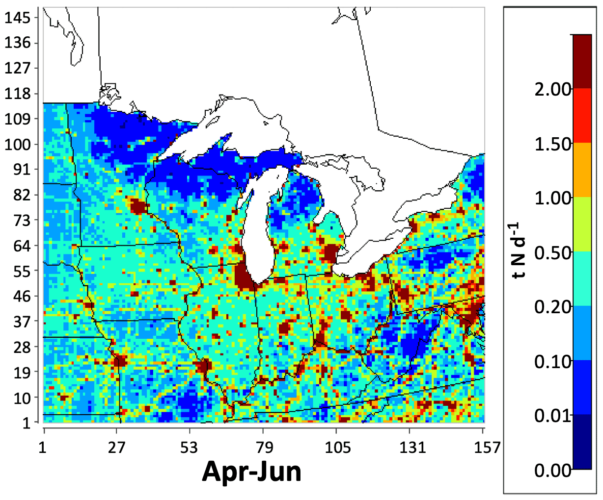
Figure 3Total NOx emission in the Midwest between April and June in tonnes of nitrogen per day (t N d−1). High NOx emissions are associated with major urban areas such as Chicago, Detroit, Minneapolis-St Paul, Kansas City, St. Louis, Indianapolis, and Louisville.
The April to June NOx emissions ranged from less than 0.01 t N d−1 to more than 15 t N d−1, with the seasonal grid average of 0.904 t N d−1. This average agrees well with estimates in previous studies for the United States, which were between 0.81 and 1.02 t N d−1 (Dignon and Hameed, 1989; Farrell et al., 1999; Selden et al., 1999; Xing et al., 2012). Within 75 % of the geographic domain, the NOx emissions are relatively low, ranging from between 0 and 0.5 t N d−1 (Fig. S3). Geographically, these grids are in rural areas some distance away from metropolitan areas and highways (Fig. 3). NOx emissions within about 20 % of the grids are relatively moderate, ranging between 0.5 and 2.0 t N d−1 (Fig. S3). Geographically, these grids are mainly located along major highways and areas with medium population densities (Fig. 3). Urban centers comprise about 5 % of the grids within the geographic domain, and these have high NOx emissions rates, ranging between 2.0 and 15.0 t N d−1 (Fig. S3). The metropolitan area's average is 5.03 t N d−1, which is nearly 14 times the average emission rate over the rest of the grids within the geographic domain (0.37 t N d−1) due to the high vehicle density associated with high population. The highest emission rates are located within large cities as well as the edge of the east coast metropolitan area (Fig. 3). Summing the NOx emissions among the grids that encompass these major midwestern cities yields city-level NOx emission rates that vary from 61.2 t N d−1 (Louisville, KY) to 634.1 t N d−1 (Chicago, IL). These city-level NOx emission rates (Table S4) agree well with estimates derived from the Ozone Monitoring Instrument (Lu et al., 2015). Grids containing power plants are significant NOx hotspots within the geographic domain. These account for less than 1 % of the grids, but the NOx emissions from a single grid that contains a power plant can be as high as 93.4 t N d−1. Geographically, the power plants are mainly located along the Ohio River valley, near other water bodies, and often close to metropolitan areas (Fig. 3). The NOx emission rates of the major power plants within the Midwest simulated by SMOKE (Table S5) match well with the measurement from the Continuous Emission Monitoring System (CEMS) (de Foy et al., 2015; Duncan et al., 2013; Kim et al., 2009). The geographic distribution of grid-level annual NOx emission density in our simulation also agrees with the county-level annual NOx emission density discussed in the 2002 NEI booklet (Fig. S4; United States Environmental Protection Agency, 2018b).
We next examine the spatial heterogeneity of the NOx source fractions (Fig. 4) for the same time period (April to June). The NOx fraction (f) is defined as the amount of NOx from a source category (s) normalized to total NOx (fs= NOx(source) NOx(total)). The fraction for anthropogenic NOx emission is defined as the amount of NOx from a source category normalized to the sum of NOx emission from anthropogenic sources (fs= NOx(source) (NOx(total)-NOx(biogenic))) Since the δ15NOx is determined by the NOx emission fractions within each grid, it is important to understand where in the domain these fractions differ and why. The area sources, which mainly consist of off-road vehicles, agriculture production, residential combustion, and industrial processes, which are individually too low in magnitude to report as point sources, are fairly uniform in their distribution across the domain.

Figure 4The geographical distribution of the fraction of NOx emission from each SMOKE processing category (area, biogenic, mobile, and point) over each grid throughout the Midwest between April and June based on NEI 2002.
The SMOKE simulation shows that the fs varies significantly across the domain. The average area NOx emission fraction (farea) was 0.271 for total NOx emission and 0.290 for anthropogenic NOx emission within the Midwest from April to June. The farea values show a clear spatial variation and range from 0.125 to 0.5 over about 75 % of the grids (Fig. S5). Geographically, the grids with relatively higher farea are in the rural area away from highways, where agriculture is the most common land use classification. In the states of Wisconsin and Missouri, the farea is slightly lower due to the higher fraction of NOx emission from biogenic sources (fbiog). In the states of Pennsylvania and Michigan, the farea is slightly lower due to the higher fraction of NOx emission from mobile sources (fmobile). In addition, the grids with farea greater than 0.75 are mainly located along the Mississippi River and Ohio River, due to wastewater discharge. The fbio shows a clear spatial variation and is highest in the western portion of the domain (Fig. 4). The fbio from April to June is less than 0.5 in more than 90 % of the grids within the geographic domain, with the average of 0.065 (Fig. S5). Geographically, the grids with relatively high fbio are located in the western regions of the Midwest, away from cities and highway where the density of agricultural acreage and natural vegetation is high. Furthermore, the lowest fbio values occur in the megacities and along the highways, which agrees well with the land use related to the biogenic emission. The April to June SMOKE simulation shows fmobile of 0.325 for total NOx emission and 0.347 for anthropogenic NOx emission. The fmobile shows a clear spatial variation, with relatively higher fmobile located in major metropolitan regions and along the highways, where vehicles have the highest density. The value of fmobile within the geographic domain distributes evenly on the histogram (Fig. S5). Based on the SMOKE simulation, the fraction of NOx emission from point sources (fpoint) is 0.339 for total NOx emission and 0.363 for anthropogenic NOx. The fpoint values are obviously highest in grids where the power plants are located, mainly along the Ohio River valley and near other water bodies close to metropolitan areas. The point sources occupy only 4 % of the domain grids, and about one-quarter of the power plants are not on the same grids as highways; thus these grids have a fpoint>0.9 NOx.
3.2 Simulated spatial variability in δ15NOx
Using these NOx emission source fractions, the δ15NOx values were simulated, and the spatial heterogeneity of δ15NOx for a single time period is discussed. The “emission only” simulation of δ15NOx values (at 06:00 UTC on 26 July) ranged from −34.3 ‰ to 14.9 ‰ (Fig. 5a). The majority of the grids have δ15NOx values lower than −16.3 ‰, which is due to biogenic NOx emissions (−34.3‰) in sparsely populated areas where intensive agriculture dominates the land use (Fig. 5a). The δ15NOx values for grids containing big cities mainly ranged between −8.75 ‰ and −5 ‰ due to the higher fraction of NOx emission from on-road vehicles (−2.7‰). Similarly, the δ15NOx values for grids ranging between −8.75 ‰ and −5 ‰ resolve major highways. The highest value of δ15N occurs at the grids, where the coal-fired EGUs (+15‰) and hybrid-fired EGUs are the dominant NOx source (Fig. 5a).
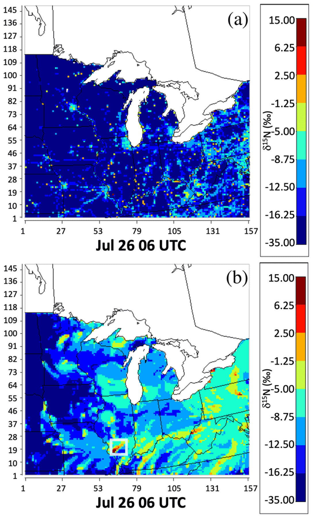
Figure 5The δ15N values of NOx emission (a emission only scenario) and the δ15N values of atmospheric NOx based on NEI 2002 and 2016 meteorology (b emission + transport scenario), at 06:00 UTC on 26 July, are presented by color in each grid. The warmer the color, the higher the δ15N values of atmospheric NOx. The feature of the transport inside the white box is shown in Fig. 6.
The effect of atmospheric mixing on the δ15NOx spatial distribution was then taken into account by coupling the 15NOx emissions to the meteorology simulation. There are significant differences between δ15NOx values in the emission only (Fig. 5a) and the emission + transport (Fig. 5b) simulations. While emission only δ15N pattern shows biogenic NOx emissions dominating the spatial domain, anthropogenic emissions become dominant over most of the grids in the emission + transport simulations, especially for the grids located around major cities and power plants. In general, as isotopically heavier urban NOx disperses, the grid average increases from −20.2 ‰ under the emission only scenario to −11.5 ‰ under the emission + transport scenario. Similarly, the NOx emitted along major highways is transported to the surrounding grids, so that the atmospheric NOx at the grids around the major highways becomes isotopically heavier relative to the emission only scenario. We define Δδ15Ntransport as the δ15N difference between emission only and emission + transport scenarios. An example of the Δδ15Ntransport effect can be seen in grids encompassing a plume emanating from southern Illinois' Baldwin Energy Complex (marked with a transparent white box in Fig. 5b) that uses subbituminous coal and bituminous coal as its major energy source. The Δδ15Ntransport in the regions is altered as a function of distance away from the EGU. In this time snapshot (06:00 UTC on 26 July), the northeastwards-propagating plume of NOx emission from the EGU creates higher δ15NOx over 135 km away (Fig. 6).
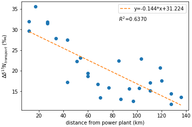
Figure 6The Δδ15Ntransport along the plume (colored in dark red to orange inside the white box in Fig. 5b) over the distance from the Baldwin Energy Complex power plant (located at the southwestern border of Illinois).
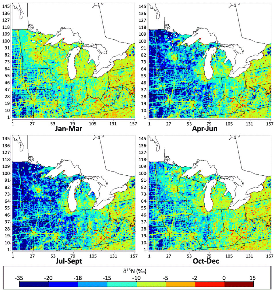
Figure 7The geographical distribution of the δ15N value of total NOx emissions in each season (winter: January–March; spring: April–June; summer: July–September; fall: October–December) in per mil (‰) throughout the Midwest simulated by SMOKE, based on NEI 2002.
3.3 Seasonal variation in δ15NOx
We next examine the temporal heterogeneity of δ15NOx values over the domain for emission only and interpret them in terms of changes in NOx emission fractions as a function of time. The predicted δ15 NOx value for total emissions in the Midwest during each season shows a significant temporal variation (Fig. 7). The δ15NOx ranged from −35 ‰ to 15 ‰, with the annual average over the Midwest at −6.15 ‰. The maps for different seasons show the obvious changes in δ15N values over western regions of the Midwest, going from −15 ‰ to −5 ‰ in the spring to −35 ‰ to −15 ‰ in the summer. In order to qualitatively analyze the changes in δ15NOx among each season, the values over the grids (Fig. 7) were organized into histograms (Fig. S6). The grids with δ15NOx between −35 ‰ and −18 ‰ increase dramatically from less than 10 % during fall (October–December) and winter (January–March) to more than 20 % during spring (April–June) and summer (July–September). The grids with δ15NOx between −18 ‰ and −2 ‰ decrease from around 90 % during fall and winter to around 75 % during spring and summer. The significant temporal variation in the δ15NOx during different seasons can be quantitatively explained by changing fractions of NOx emission from the biogenic source in any grid (Fig. S7) using Eq. (6). Unlike other NOx emission sources, the fraction of NOx emission from biogenic sources changes significantly among each season within the geographic domain, especially over the rural areas (Fig. S7).
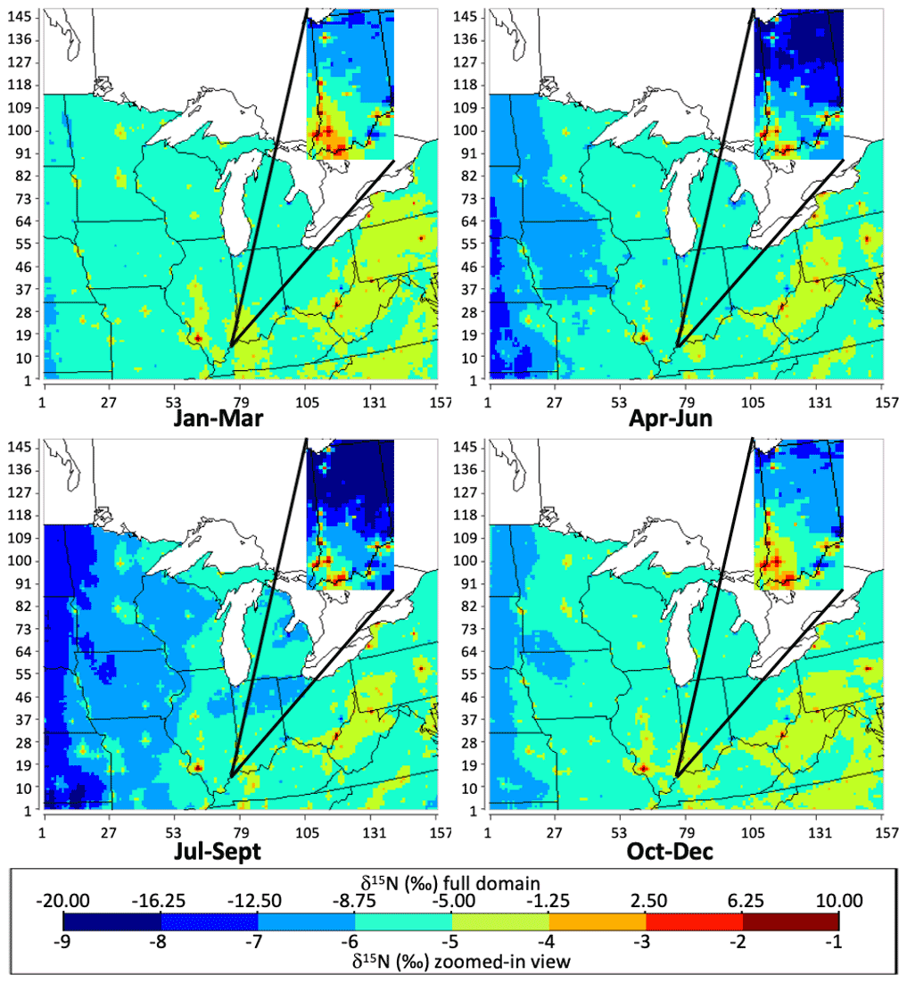
Figure 8The geographical distribution of the δ15N value of atmospheric NOx in each season (winter: January–March; spring: April–June; summer: July–September; fall: October–December) in per mil (‰) throughout the Midwest (with zoomed-in view focusing on Indiana), simulated by CMAQ, based on NEI 2002 and 2016 meteorology.
To qualitatively analyze the changes in the fraction of NOx emission from biogenic sources among each season, the distributions of the fractions among the same cutoffs as the maps in Fig. S7 were shown in the histograms (Fig. S8). In general, the distribution of the fraction shifts to higher values during spring (April–June) and summer (July–September), indicating the increase of biogenic emissions. During this period, the surface sunlight hours, temperature, and precipitation are relatively higher, and as a result, the canopy coverage of the plants becomes higher, which leads to the increase of the NOx emission from biogenic sources (Pierce, 2001; Vukovich and Pierce, 2002; Schwede et al., 2005; Pouliot and Pierce, 2009; United States Environmental Protection Agency, 2018a). Besides this, the fertilizer application during this period also increases soil NOx emissions (Li and Wang, 2008; Felix and Elliott, 2014). As a result, the distribution of δ15NOx shifts to lower values during these periods (Fig. 7). The percentage of the grids with the fraction of biogenic emission less than 0.125 decreases dramatically from more than 50 % during fall (October–December) and winter (January–March) to less than 35 % during spring (April–June) and summer (July–September). As the NOx emission from biogenic source becomes dominant, the percentage of the grids with δ15NOx between −35 ‰ and −18 ‰ increases, while the percentage of the grids with values between −18 ‰ and −2 ‰ decreases, which sufficiently explains the trends shown in Fig. 7.
The temporal variation in atmospheric δ15NOx is also controlled by the propagation of NOx emissions, which varies seasonally. The temporal heterogeneity of atmospheric δ15NOx under the emission + transport scenario is interpreted in terms of changes in the propagation of NOx emission as a function of time. The predicted seasonal average δ15NOx in the Midwest shows significant variations (Fig. 8). On an annual basis, the emission + transport average δ15NOx value was −6.10 ‰, which is similar to the emission only average range, but the range (−19.2 ‰ to 11.6‰) was narrower due to NOx transport and mixing. The maps for different seasons show the obvious changes in δ15N values over western regions of the Midwest, from −8.75 ‰ to −5 ‰ in fall and winter to −16.25 ‰ to −12.5 ‰ in spring and summer. The spatial heterogeneity of the δ15NOx under the emission + transport scenario (Fig. 8) was compared to that under the emission only scenario (Fig. 7). The difference was defined as Δδ15Ntransport (Fig. S9) and had values that ranged from −21.9 ‰ to 31.2 ‰, with an average of 4.9 ‰. The grids with Δδ15Ntransport between −5 ‰ and 0 ‰ are the urban areas and decrease slightly from about 11 % during fall (October–December) and winter (January–March) to 10 % during spring (April–June) and summer (July–September). The grids with Δδ15Ntransport between 0 ‰ and 5 ‰ are typically in the rural areas that are impacted by the urban NOx emissions and decrease dramatically from more than 50 % during fall and winter to less than 40 % during spring and summer. The grids with Δδ15Ntransport greater than 5 ‰ are in the rural areas obviously impacted by the urban NOx emission and increase dramatically from less than 40 % during fall and winter to more than 50 % during spring and summer. Therefore, the impacts from transport and mixing are more obvious during spring and summer (Fig. S10).
The planetary boundary layer (PBL) height is an effective indicator showing whether the pollutants are under synoptic conditions which are favorable for the dispersion, mixing, and transport after being emitted into the atmosphere (Oke, 2002; Shu et al., 2017; Liao et al., 2018; Miao et al., 2019). Comparing the distributions of Δδ15Ntransport values (Fig. S9) with the corresponding PBL height (Fig. S11) for each season, the effects of PBL height on the propagation of the air mass are clearly shown. NOx emitted by power plants is much higher than the emission rates at the surrounding grids and is a hotspot that impacts the δ15N values on the surrounding grids. As PBL increases, the emitted NOx from power plant mixes more effectively with the surrounding grid; thus there are higher δ15NOx values along the power plant plume transect. The PBL height changes significantly among each season within the geographic domain, especially over Minnesota, Wisconsin, and Iowa (Fig. S11). The PBL height over these areas increases from less than 250 m above the ground level to more than 625 m a.g.l., during spring and summer, which creates a more favorable synoptic condition for the dispersion, mixing, and transport of the pollutants after being emitted into the atmosphere. As a result, the difference in δ15N values shifts to higher values, showing the stronger effect of atmospheric processes during spring and summer. In order to qualitatively analyze how PBL height affects the δ15NOx along power plant plumes, the domain average PBL height for each month was plotted against δ15NOx (Fig. 9a). The δ15N values along the power plants' plumes and PBL heights over the domain have the same seasonal trend. Interestingly, the “turning point” of the δ15N values is about 1 month later than the turning point of the PBL heights. The scatter plot (Fig. 9b) shows a strong positive correlation (R2=0.85) between the domain average PBL height and average δ15N value along the power plants' plumes. The positive correlation between PBL height and propagation of air mass, indicated by the evolution of atmospheric δ15NOx in this study, agrees well with the corresponding measurement in megacities in China from previous studies (Shu et al., 2017; Liu et al., 2018; Liao et al., 2018).
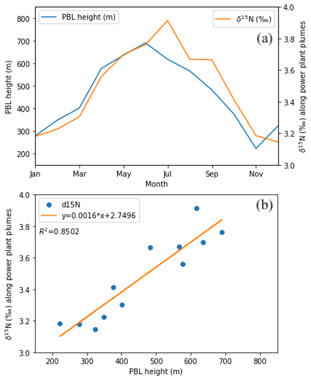
Figure 9The time series plot (a) and the scatter plot (b) of the domain average PBL height (m) and the average δ15N (‰) value of atmospheric NOx along the plumes of power plants during each month throughout the Midwest simulated by CMAQ, based on NEI 2002 and 2016 meteorology.
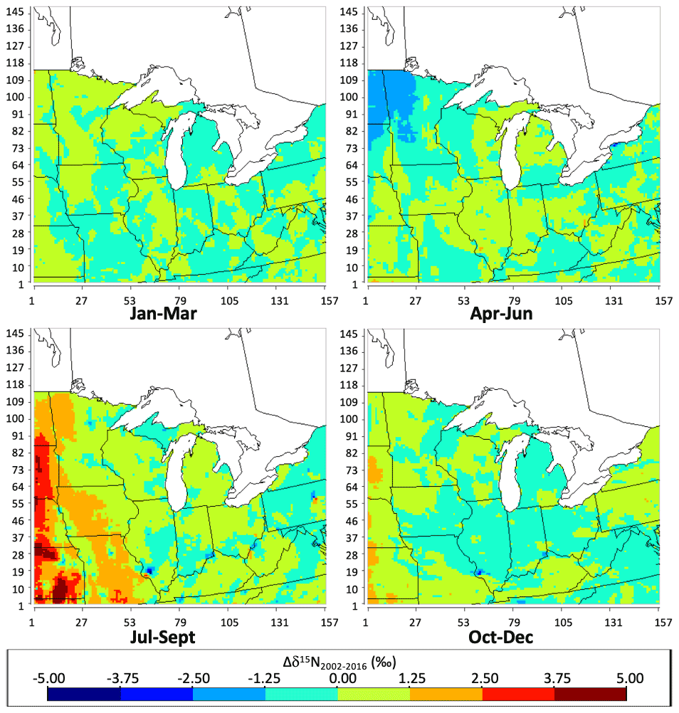
Figure 10The difference between the δ15N (‰) value of atmospheric NOx based on 2016 meteorology and 2002 meteorology (Δδ15N2002–2016) during each season (winter: January–March; spring: April–June; summer: July–September; fall: October–December), throughout the Midwest, simulated by CMAQ.
3.4 The simulations based on different meteorology input datasets
The spatial heterogeneity of the δ15NOx using 2016 meteorology input dataset was compared to that using 2002 meteorology (Fig. S13). Overall, the simulated δ15NOx using 2002 meteorology has the similar geographic distribution and seasonal trend as the 2016 simulation. The difference was defined as Δδ15N2002–2016 (Fig. 10) and had values that ranged between −1.25 ‰ and +1.25 ‰ over most of the grids. However, in the western part of the domain, where the biogenic NOx emission is dominant, the more positive Δδ15N2002–2016 values (up to 5 ‰) occur during summer and fall. On the other hand, the more negative Δδ15N2002–2016 values (up to −5 ‰) occur along the power plant plume during the same period. The spatial heterogeneity of Δδ15N2002–2016 indicates how climate change alters the δ15NOx. If we have enough input datasets to generate and compare the seasonal/monthly δ15NOx over the past 20+ years, the impacts of anomalies in each meteorology variables could be explored. For the current dataset, a similar comparison between the δ15NOx and the corresponding PBL height was conducted for the simulation based on 2002 meteorology (Fig. S14) to show how PBL height changes the evolution of δ15NOx. Under the 2002 meteorology, lower PBL height during the winter caused surface δ15NOx values along the power plants' plumes to be lower relative to 2016 meteorology. On the other hand, due to the higher PBL height during spring and summer 2002, the δ15N values decreased through July before ending with relatively higher δ15N values in December. The scatter plot for the simulation based on 2002 meteorology (Fig. S14b) also shows a strong positive correlation between the domain average PBL height and average δ15N value along the power plants' plumes, with R2=0.78. The videos of atmospheric δ15NOx on an hourly basis throughout the years 2002 and 2016 are available on http://www.zenodo.org (last access: 8 December 2021) (https://doi.org/10.5281/zenodo.4311986, Fang, 2020b).
3.5 The simulation over the extracted domain
Analysis of whether there was a difference between the extracted-domain simulation (Fig. 2) and full-domain simulation was conducted by defining Δδ15Nextracted-full and assessing the bias due to the motion of the air mass across the domain boundary (Fig. S17). The Δδ15Nextracted-full values ranged between −0.25 ‰ and +0.25 ‰ over most of the grids, showing that the difference between the extracted-domain simulation and full-domain simulation of δ15N values is usually trivial. However, near the southern border of the extracted domain, Δδ15Nextracted-full values are close to +0.75 ‰ (fall and winter) and close to +1.00 ‰ (spring and summer), suggesting the extracted domain may be required for accurate δ15NOx simulations
3.6 The role of enhanced NOx loss
The emission + transport + enhanced NOx loss simulations significantly alter the δ15NOx relative to the “normal deposition” scenarios. Again, the enhanced NOx loss cases are removing NOx at rates similar to those by removal via its conversion into HNO3. Thus, the NOx deposited is ∼ δ15NO (assuming no photochemical isotope effects), and the δ15NOx is that in the residual NOx. The impact of enhanced NOx loss on the residual NOx was assessed using Δδ15Nhi-no, the difference between the δ15NOx values under the “enhanced NOx loss” and “no deposition” scenarios. The Δδ15Nhi-no range was ±4 ‰ and was especially obvious downwind of the locations with large emission rates, such as power plants or megacities (Fig. 11). This can be explained in a similar fashion to the no deposition scenarios (Fig. S18a), where the dispersion of the isotopically heavier NOx emission from big cities, major highways, and power plants elevated the δ15NOx values in rural areas, and the dispersion of the isotopically lighter biogenic NOx emission lowered the δ15NOx values in the surrounding grids located in the suburb of major cities (Fig. S18b). When enhanced NOx loss is used, the transport, mixing, and dispersion of local NOx emissions are restricted to a smaller geographical extent (Fig. S18b), leading to different δ15NOx values relative to no deposition. The temporal heterogeneity of Δδ15Nhi-no over the domain was examined and the impact of enhancing deposition rates of NOx on the δ15N of atmospheric NOx was explored on a seasonal basis (Fig. 12). The seasonal Δδ15Nhi-no values range from −3.67 ‰ to 5.34 ‰, with an average of 0.51 ‰. The overall pattern of the Δδ15Nhi-no values shows that due to deposition, the atmospheric NOx became isotopically lighter over the majority of the grids since EGU and vehicle NOx is not being transported as far. Conversely, in grids that contain or surround power plants and big cities, the δ15NOx increases because it is not as effectively mixing with low δ15NOx from nearby grids. The enhanced NOx loss simulation was used as a proxy to present the isotope effects associated with the “pseudo photochemical transformation” of NOx into NOy. The complete isotope effect of tropospheric photochemistry will be addressed in future work, which incorporates 15N into the chemical mechanism of CMAQ for the simulation.
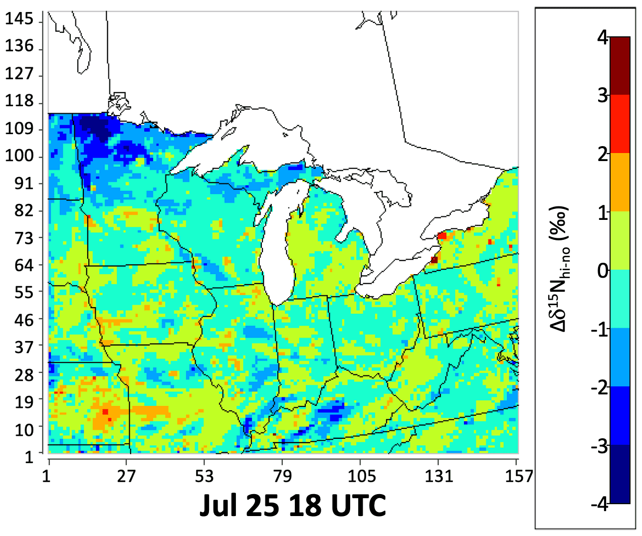
Figure 11The Δδ15Nhi-no values at 18:00 UTC on 25 July.
The δ15NOx values of dry deposition (a proxy for δ15NO) simulated by CMAQ show similar monthly variations and seasonal trends to SMOKE (Fig. S22). The ranges of δ15NOx values within each month were narrower, compared to the simulation from SMOKE, with a minimum during February (−8.7 ‰ to −4.4 ‰) and a maximum during August (−11.8 ‰ to −4.2 ‰). The seasonal trend shows low δ15NOx values in deposition during summer, with the median around −7.4 ‰ and slightly higher values during winter (median around −6.0 ‰). Therefore, the CMAQ simulation inherits the monthly variations and seasonal trends from SMOKE, while the atmospheric NOx becomes isotopically heavier, after taking atmospheric mixing and transport into account. As mentioned above, most of the NADP sites are located away from big cities and power plants. Thus, the atmospheric mixing and transport led to the isotopically heavier atmospheric NOx.
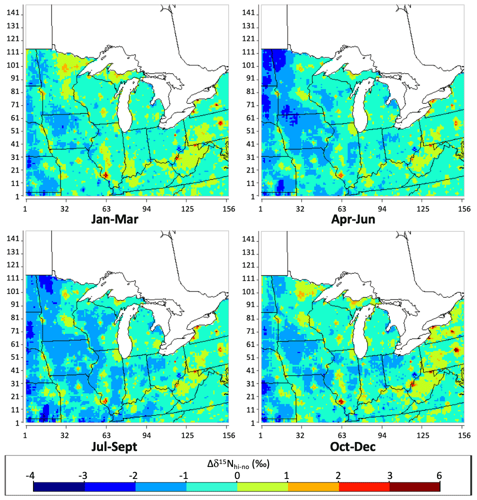
Figure 12The difference between the δ15N (‰) values of atmospheric NOx under the enhanced NOx loss scenario and no deposition scenario (Δδ15Nhi-no) during each season (winter: January–March; spring: April–June; summer: July–September; fall: October–December), throughout the Midwest, simulated by CMAQ, based on NEI 2002 and 2016 meteorology.
3.7 Model–observation comparison of δ15NOx
In order to evaluate the SMOKE/CMAQ simulations of atmospheric δ15NOx, they were compared to two recent studies of δ15NOx. The first comparison was relative to rainwater measurements in West Lafayette, IN, from 9 July to 5 August 2016 (Walters et al., 2018). The measured δ15NOx values ranged from −33.8 ‰ to 0.2 ‰, with a median of −11.2 ± 8.02 ‰. Under the emission + transport + enhanced NOx loss scenario using 2016 meteorology, the simulated δ15NOx mean (−7.9 ± 2.19 ‰) was 3.3 ‰ less negative than the observations, and the range (−15.9 ‰ to −3.7 ‰) was about half that in the observations (Fig. 13, top, Table S7). The predicted δ15NOx was similar regardless of whether 2016 or 2002 meteorology was used but was closer to the measured values compared to the emission only simulations (Fig. 13, top). It is not surprising that the measurements are more negative than the observations because the model does not account for isotope fractionation during the conversion of NOx into NOy. Our previous work has shown that the photochemical isotope effect enriches NOy and depletes NOx (Fang et al., 2021; Walters and Michalski, 2015), and thus the lower measured δ15NOx relative to model is consistent with this isotopic depletion. Our model simulations were also compared to on-road vehicle plume measurement along Midwest highways from 8 to 18 August 2015 (Miller et al., 2017). The box plot also shows more accurate estimation of δ15N after considering the atmospheric mixing with the emission from surrounding grids (Fig. 13, bottom). Using the emission only scenario, the simulated δ15NOx mean was about 3 ‰ more negative than the observations. The predicted δ15NOx under the emission + transport + enhanced NOx loss scenario for these samples along Midwest highways was closer to the measured values, compared to the emission only simulations, regardless of whether 2016 or 2002 meteorology was used. The modeled values are quite close to the observations, suggesting that the photochemical isotope effect is small for these samples. This is not surprising given they were collected on major highways where NOx concentrations are high and the timescale between collection and emission is small, and thus only a small fraction of emitted NOx would have been converted to NOy, minimizing the photochemical isotope effect.
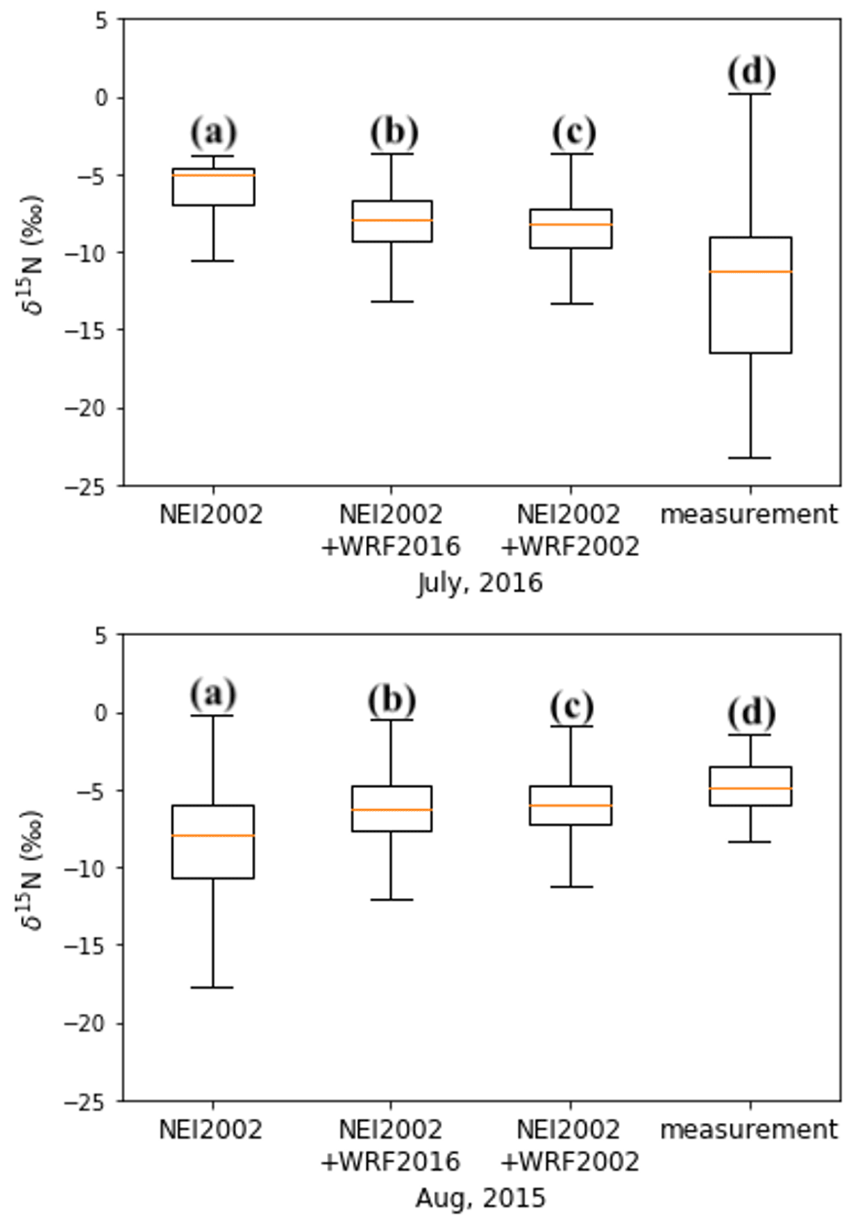
Figure 13The δ15NOx distributions at Lafayette, IN (top), and along Midwest highways (bottom), simulated by SMOKE (a), CMAQ based on 2016 (b) and 2002 meteorology (c), compared with the measured δ15NOx (d) (box: lower quartile, median, upper quartile; whisker: lower extreme, upper extreme)
The 30-fold enhanced NOx loss (see methods) was used to simulate the δ15N value of NO deposition (δ15NO) that was then compared to observations (Fig. 14). As previously noted, rather than explicitly converting NOx into NOy via the chemical mechanism in CMAQ, which would require writing an isotope-enabled chemical scheme with appropriate rate constants, we amplified NOx deposition as a surrogate. This amplification reduced the NOx lifetime to about 1 d; thus by calculating the δ15NOx in the deposition fraction, as opposed to residual NOx in the atmosphere, we are approximating the δ15NO in deposition. The simulated δ15NO was compared to NO collected at NADP sites within Indiana, Illinois, and Ohio in the year 2002 (Table S4). The NEI 2002 and WRF2002 were used for the SMOKE emission model and CMAQ simulations, respectively. The value of deposition was calculated by δ15NONOxh, where fNOxh is the hourly mole fraction of NOx isotopologue deposited (fNOxh= NOxh NOxT), and δ15NOxh is the δ15N value of NOx in deposition. The total NOx deposited (NOxT) used to calculate fNOxh was the amount deposited 5 d prior to the sampling date since the NADP deposition collection integrates the week.
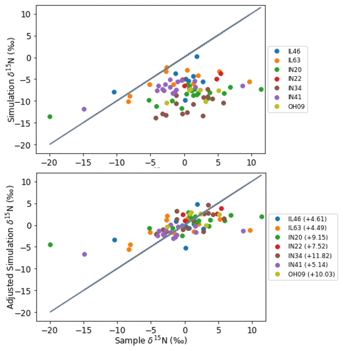
Figure 14The emission + transport + enhanced NOx loss CMAQ-predicted δ15N value of NOx deposition using NEI 2002 and 2002 meteorology compared to the measured δ15N of rain NO at NADP sites within IN, IL, and OH. The photochemical isotope enrichment factor (‰) correction used for each site is noted in the legend.
The δ15N values of NOx deposition simulated by CMAQ under the emission + transport + enhanced NOx loss scenario at each site were compared with the measurements of δ15N values of NO3 from prior studies (Mase, 2010; Riha, 2013). While the scatter plot shows a moderate positive correlation between observed and simulated δ15NO, the simulated value is consistently lighter than the sample δ15NO (Fig. 14, top). The magnitude of this negative bias varies among the NADP sites (Fig. S23) and is attributed to isotope fractionation during the conversion NOx into NOy, which enriches NO (Fang et al., 2021; Walters and Michalski, 2015). Globally, this enrichment has been estimated at 3.9 ± 1.8 ‰ (Song et al., 2021). But this enrichment is a function of NOx, volatile organic compounds (VOCs), and oxidant loading, as well as temperature and photolysis rate (Fang et al., 2021), and is not expected to be the same at each NADP site. After adjusting the simulated δ15N by raising the values by the average of the difference between sample δ15N and simulated δ15N for each site, the scatter plots of sample δ15N vs. simulated δ15N fit well into the 1 : 1 line (Fig. 14, bottom). The complete 15N-incorporated chemical mechanisms will be explored in a future study.
The evolution of δ15N values along the “journey” of atmospheric NOx were traced, using our 15N-incorporated SMOKE and CMAQ. The δ15NOx under the emission only scenario was simulated by SMOKE, using the NOx emissions from NEI emission sectors and the corresponding δ15N values from previous research. The SMOKE simulation indicates that the NOx emission from biogenic sources is the key driver for the variation of δ15N, especially among the Midwestern NADP sites. The uncertainties in the δ15NOx emission are less than 5 ‰ over the majority of the grids within the Midwest, which were well below the difference among the assigned δ15NOx values for different NOx emission sources (Fig. S24). The δ15NOx under the emission + transport scenario was simulated by CMAQ, using the 15N-incorporated emission input dataset generated from SMOKE, as well as the meteorology input dataset generated from WRF and MCIP. The CMAQ simulation indicates that the PBL height is the key driver for the mixture of anthropogenic and natural NOx emission, which deepens the gap between δ15N of atmospheric NOx and NOx emission. The δ15NOx under the emission + transport + enhanced NOx loss scenario was simulated by enhancing NOx deposition in CMAQ simulation, to show how lifetime chemistry alters δ15NOx values before it can be transported along significant distances, assuming no isotope fractionation during chemical conversion or deposition.
The simulations under emission only scenario and emission + transport + enhanced NOx loss scenario were compared to the measurements in West Lafayette, Indiana. The simulated δ15N agreed well with the seasonal trend and monthly variation. The simulated δ15NOx under the emission only scenario was less negative than the corresponding measurements in West Lafayette, IN, taken from July to August 2016. Thus, if we only consider the effects from NOx emission sources, it is possible that the emissions from soil, livestock waste, off-road vehicles, and natural-gas power plant in West Lafayette, IN, are underestimated, and the emissions from the on-road vehicles and coal-fired power plants in West Lafayette, IN, are possibly overestimated. The simulated δ15NOx under the emission + transport + enhanced NOx loss scenario was about 3 ‰ closer to the corresponding measurements in West Lafayette, IN, compared to the emission only simulations. The simulations under the emission + transport + enhanced NOx loss scenario were also compared to the measurements of δ15NO from NADP sites within Indiana, Illinois, Ohio, and Kentucky. The sample-by-sample comparison shows a moderate positive correlation between observed and simulated δ15NO, with the negative bias varying among the NADP sites. This bias is attributed to isotope fractionation during the conversion of NOx into NOy, affected by different NOx, VOCs, and oxidant loading, as well as temperature and photolysis rate, at each NADP site. Therefore, future work will explore how tropospheric photochemistry alters δ15NOx by incorporating 15N into the chemical mechanism of CMAQ and comparing the simulation with the corresponding measurements. With the validation of our nitrogen isotopes incorporating CMAQ, the NOx emission inventories could be effectively evaluated and improved.
The source code for SMOKE version 4.6 is available at https://github.com/CEMPD/SMOKE/releases/tag/SMOKEv46_Sep2018 (last access: 1 March 2021) (https://doi.org/10.5281/zenodo.4480334, Baek and Seppanen, 2021). The source code for CMAQ version 5.2.1 is available at https://github.com/USEPA/CMAQ/tree/5.2.1 (last access: 1 May 2018) (https://doi.org/10.5281/zenodo.1212601, US EPA Office of Research and Development, 2018). The detailed simulation results for δ15N of the NOx emission based on 2002 and 2016 versions of the National Emission Inventory and the associated Python codes are archived on Zenodo (https://doi.org/10.5281/zenodo.4048992, Fang, 2020a). The input datasets for WRF simulation are available at https://www.ncei.noaa.gov/data/ (National Centers for Environmental Information, 2018). The detailed simulation results for δ15N of atmospheric NOx under all scenarios discussed in this paper and the CMAQ-based c-shell script for generating BCON for the extracted-domain simulation are archived on Zenodo (https://doi.org/10.5281/zenodo.4311987, Fang, 2020b).
The supplement related to this article is available online at: https://doi.org/10.5194/gmd-15-4239-2022-supplement.
HF and GM were the investigator for the project and organized the tasks. HF developed the model codes, performed the simulation to incorporate 15N into SMOKE outputs and generate δ15N values and reconstruct CMAQ by incorporating 15N, and performed the simulation to generate δ15N values. GM helped HF in interpreting the results. HF prepared the manuscript with contributions from all co-authors.
The contact author has declared that neither they nor their co-author has any competing interests.
Publisher's note: Copernicus Publications remains neutral with regard to jurisdictional claims in published maps and institutional affiliations.
We would like to thank the Purdue Research Foundation, the Purdue Climate Change Research Center, and the National Science Foundation (AGS award 1903646) for providing funding for the project. We would like to thank Scott Spak from the School of Urban and Regional Planning, University of Iowa, for simulating SMOKE using NEI 2002. We would like to thank Tomas Ratkus from the Department of Earth, Atmospheric, and Planetary Sciences and Steven Plite and Frank Bakhit from the Rosen Center for Advanced Computing, Purdue University, for setting up CMAQ on Purdue Research Computing for this project.
This research has been supported by the Purdue Research Foundation, the Purdue Climate Change Research Center, and the National Science Foundation (AGS award 1903646).
This paper was edited by Slimane Bekki and Christian Folberth and reviewed by two anonymous referees.
Almaraz, M., Bai, E., Wang, C., Trousdell, J., Conley, S., Faloona, I., and Houlton, B. Z.: Agriculture is a major source of NOx pollution in California, Sci. Adv., 4, eaao3477, https://doi.org/10.1126/sciadv.aao3477, 2018.
Ammann, M., Siegwolf, R., Pichlmayer, F., Suter, M., Saurer, M. and Brunold, C.: Estimating the uptake of traffic-derived NO2 from 15N abundance in Norway spruce needles, Oecologia, 118, 124–131, https://doi.org/10.1007/s004420050710, 1999.
Baek B. H. and Seppanen C.: CEMPD/SMOKE: SMOKE v4.8.1 Public Release (January 29, 2021), Zenodo [data set], https://doi.org/10.5281/zenodo.4480334, 2021.
de Foy, B., Lu, Z., Streets, D. G., Lamsal, L. N., and Duncan, B. N.: Estimates of power plant NOx emissions and lifetimes from OMI NO2 satellite retrievals, Atmos. Environ., 116, 1–11, https://doi.org/10.1016/j.atmosenv.2015.05.056, 2015.
Dignon, J. and Hameed, S.: Global emissions of nitrogen and sulfur oxides from 1860 to 1980, J. Air Waste Manage., 39, 180–186, https://doi.org/10.1080/08940630.1989.10466519, 1989.
Duncan, B. N., Yoshida, Y., De Foy, B., Lamsal, L. N., Streets, D. G., Lu, Z., Pickering, K. E., and Krotkov, N. A.: The observed response of Ozone Monitoring Instrument (OMI) NO2 columns to NOx emission controls on power plants in the United States: 2005–2011, Atmos. Environ., 81, 102–111, https://doi.org/10.1016/j.atmosenv.2013.08.068, 2013.
Elliott, E. M., Kendall, C., Boyer, E. W., Burns, D. A., Lear, G. G., Golden, H. E., Harlin, K., Bytnerowicz, A., Butler, T. J., and Glatz, R.: Dual nitrate isotopes in dry deposition: Utility for partitioning NOx source contributions to landscape nitrogen deposition, J. Geophys. Res.-Biogeo., 114, G04020, https://doi.org/10.1029/2008JG000889, 2009.
Elliott, E. M., Kendall, C., Wankel, S. D., Burns, D. A., Boyer, E. W., Harlin, K., Bain, D. J., and Butler, T. J.: Nitrogen isotopes as indicators of NOx source contributions to atmospheric nitrate deposition across the midwestern and northeastern United States, Environ. Sci. Technol., 41, 7661–7667, https://doi.org/10.1021/es070898t, 2007.
Fang, H.: Simulating δ15N of NOx emission within Midwestern United States, Zenodo [data set], https://doi.org/10.5281/zenodo.4048993, 2020a.
Fang, H.: Simulating δ15N of atmospheric NOx with the impacts from atmospheric processes, Zenodo [data set], https://doi.org/10.5281/zenodo.4311987, 2020b.
Fang, H., Walters, W. W., Mase, D., and Michalski, G.: iNRACM: incorporating 15N into the Regional Atmospheric Chemistry Mechanism (RACM) for assessing the role photochemistry plays in controlling the isotopic composition of NOx, NOy, and atmospheric nitrate, Geosci. Model Dev., 14, 5001–5022, https://doi.org/10.5194/gmd-14-5001-2021, 2021.
Farrell, A., Carter, R., and Raufer, R.: The NOx Budget: Market-based control of tropospheric ozone in the northeastern United States, Resour. Energy Econ., 21, 103–124, https://doi.org/10.1016/S0928-7655(98)00035-9, 1999.
Felix, J. D. and Elliott, E. M.: The agricultural history of human-nitrogen interactions as recorded in ice core δ15N-NO, Geophys. Res. Lett., 40, 1642–1646, https://doi.org/10.1002/grl.50209, 2013.
Felix, J. D. and Elliott, E. M.: Isotopic composition of passively collected nitrogen dioxide emissions: Vehicle, soil and livestock source signatures, Atmos. Environ., 92, 359–366, https://doi.org/10.1016/j.atmosenv.2014.04.005, 2014.
Felix, J. D., Elliott, E. M., and Shaw, S. L.: Nitrogen isotopic composition of coal-fired power plant NOx: Influence of emission controls and implications for global emission inventories, Environ. Sci. Technol., 46, 3528–3535, https://doi.org/10.1021/es203355v, 2012.
Felix, J. D., Elliott, E. M., Avery, G. B., Kieber, R. J., Mead, R. N., Willey, J. D., and Mullaugh, K. M.: Isotopic composition of nitrate in sequential Hurricane Irene precipitation samples: Implications for changing NOx sources, Atmos. Environ., 106, 191–195, https://doi.org/10.1016/j.atmosenv.2015.01.075, 2015.
Fibiger, D. L., Hastings, M. G., Lew, A. F., and Peltier, R. E.: Collection of NO and NO2 for isotopic analysis of NOx emissions, Anal. Chem., 86, 12115–12121, https://doi.org/10.1021/ac502968e, 2014.
Fujita, E. M., Croes, B. E., Bennett, C. L., Lawson, D. R., Lurmann, F. W., and Main, H. H.: Comparison of emission inventory and ambient concentration ratios of CO, NMOG, and NOx in California's South Coast Air Basin, J. Air Waste Manage., 42, 264–276, https://doi.org/10.1080/10473289.1992.10466989, 1992.
Galloway, J. N., Dentener, F. J., Capone, D. G., Boyer, E. W., Howarth, R. W., Seitzinger, S. P., Asner, G. P., Cleveland, C. C., Green, P. A., Holland, E. A., Karl, D. M., Michaels, A. F., Porter, J. H., Townsend, A. R., and Vörösmarty, C. J.: Nitrogen cycles: Past, present, and future, Biogeochemistry, 70, 153–226, https://doi.org/10.1007/s10533-004-0370-0, 2004.
Garten, C. T.: Nitrogen isotope composition of ammonium and nitrate in bulk precipitation and forest throughfall, Int. J. Environ. Anal. Chem., 47, 33–45, https://doi.org/10.1080/03067319208027017, 1992.
Hall, S. J., Ogata, E. M., Weintraub, S. R., Baker, M. A., Ehleringer, J. R., Czimczik, C. I., and Bowling, D. R.: Convergence in nitrogen deposition and cryptic isotopic variation across urban and agricultural valleys in northern Utah, J. Geophys. Res.-Biogeo., 121, 2340–2355, https://doi.org/10.1002/2016JG003354, 2016.
Heaton, T. H. E.: 15N14N ratios of nitrate and ammonium in rain at Pretoria, South Africa, Atmos. Environ., 21, 843–852, https://doi.org/10.1016/0004-6981(87)90080-1, 1987.
Heaton, T. H. E.: 15N/14N ratios of NOx from vehicle engines and coal-fired power stations, Tellus B, 42, 304–307, https://doi.org/10.1034/j.1600-0889.1990.00007.x-i1, 1990.
Hoering, T.: The isotopic composition of the ammonia and the nitrate ion in rain, Geochim. Cosmochim. Ac., 2, 97–102, https://doi.org/10.1016/0016-7037(57)90021-2, 1957.
Houyoux, M.: Clean Air Interstate Rule Emissions Inventory Technical Support Document, US EPA, https://swap.stanford.edu/20140418220813/http://www.epa.gov/air/interstateairquality/pdfs/finaltech01.pdf (last access: 22 May 2018), 2005.
Ingalls, M. N.: On-road vehicle emission factors from measurements in a Los Angeles area tunnel, in: Proceedings of the Air & Waste Management Association 82nd Annual Meeting, Anaheim, California, 25–30 June 1989, 89-137.3, 1989.
Jaeglé, L., Steinberger, L., Martin, R. V., and Chance, K.: Global partitioning of NOx sources using satellite observations: Relative roles of fossil fuel combustion, biomass burning and soil emissions, Faraday Discuss., 130, 407–423, https://doi.org/10.1039/B502128F, 2005.
Johansson, C.: Pine forest: a negligible sink for atmospheric NOx in rural Sweden, Tellus B, 39, 426–438, https://doi.org/10.3402/tellusb.v39i5.15360, 1987.
Kim, S. W., Heckel, A., Frost, G. J., Richter, A., Gleason, J., Burrows, J. P., McKeen, S., Hsie, E. Y., Granier, C., and Trainer, M.: NO2 columns in the western United States observed from space and simulated by a regional chemistry model and their implications for NOx emissions, J. Geophys. Res.-Atmos., 114, D11301, https://doi.org/10.1029/2008JD011343, 2009.
Laughner, J. L. and Cohen, R. C.: Direct observation of changing NOx lifetime in North American cities, Science, 366, 723–727, 2019.
Li, D. and Wang, X.: Nitrogen isotopic signature of soil-released nitric oxide (NO) after fertilizer application, Atmos. Environ., 42, 4747–4754, https://doi.org/10.1016/j.atmosenv.2008.01.042, 2008.
Liao, T., Gui, K., Jiang, W., Wang, S., Wang, B., Zeng, Z., Che, H., Wang, Y., and Sun, Y.: Air stagnation and its impact on air quality during winter in Sichuan and Chongqing, southwestern China, Sci. Total Environ., 635, 576–585, https://doi.org/10.1016/j.scitotenv.2018.04.122, 2018.
Lighty, J. A. S., Veranth, J. M., and Sarofim, A. F.: Combustion aerosols: Factors governing their size and composition and implications to human health, J. Air Waste Manage., 50, 1565–1618, https://doi.org/10.1080/10473289.2000.10464197, 2000.
Liu, L., Guo, J., Miao, Y., Liu, L., Li, J., Chen, D., He, J., and Cui, C.: Elucidating the relationship between aerosol concentration and summertime boundary layer structure in central China, Environ. Pollut., 241, 646–653, https://doi.org/10.1016/j.envpol.2018.06.008, 2018.
Lu, Z., Streets, D. G., de Foy, B., Lamsal, L. N., Duncan, B. N., and Xing, J.: Emissions of nitrogen oxides from US urban areas: estimation from Ozone Monitoring Instrument retrievals for 2005–2014, Atmos. Chem. Phys., 15, 10367–10383, https://doi.org/10.5194/acp-15-10367-2015, 2015.
Ludwig, J., Meixner, F. X., Vogel, B., and Forstner, J.: Soil-air exchange of nitric oxide: An overview of processes, environmental factors, and modeling studies, Biogeochemistry, 52, 225–257, https://doi.org/10.1023/A:1006424330555, 2001.
Mase, D. F.: A coupled modeling and observational approach to understanding oxygen-18 in atmospheric nitrate, PhD thesis, Purdue University, United States of America, 2010.
Miao, Y., Li, J., Miao, S., Che, H., Wang, Y., Zhang, X., Zhu, R., and Liu, S.: Interaction Between Planetary Boundary Layer and PM2.5 Pollution in Megacities in China: a Review, Curr. Pollut. Reports, 5, 261–271, https://doi.org/10.1007/s40726-019-00124-5, 2019.
Miller, D. J., Wojtal, P. K., Clark, S. C., and Hastings, M. G.: Vehicle NOx emission plume isotopic signatures: Spatial variability across the eastern United States, J. Geophys. Res., 122, 4698–4717, https://doi.org/10.1002/2016JD025877, 2017.
Miller, D. J., Chai, J., Guo, F., Dell, C. J., Karsten, H., and Hastings, M. G.: Isotopic Composition of In Situ Soil NOx Emissions in Manure-Fertilized Cropland, Geophys. Res. Lett., 45, 12058, https://doi.org/10.1029/2018GL079619, 2018.
Moore, H.: The isotopic composition of ammonia, nitrogen dioxide and nitrate in the atmosphere, Atmos. Environ., 11, 1239–1243, https://doi.org/10.1016/0004-6981(77)90102-0, 1977.
National Centers for Environmental Information: Index of /data, https://www.ncei.noaa.gov/data/, last access: 1 September 2018.
Occhipinti, C., Aneja, V. P., Showers, W., and Niyogi, D.: Back-trajectory analysis and source-receptor relationships: Particulate matter and nitrogen isotopic composition in rainwater, J. Air Waste Manage., 58, 1215–1222, https://doi.org/10.3155/1047-3289.58.9.1215, 2008.
Oke, T. R.: Boundary Layer Climates, 2nd Edn., Routledge, London, UK, 2002.
Parrish, D. D.: Critical evaluation of US on-road vehicle emission inventories, Atmos. Environ., 40, 2288–2300, https://doi.org/10.1016/j.atmosenv.2005.11.033, 2006.
Pearson, J., Wells, D. M., Seller, K. J., Bennett, A., Soares, A., Woodall, J., and Ingrouille, M. J.: Traffic exposure increases natural 15N and heavy metal concentrations in mosses, New Phytol., 147, 317–326, https://doi.org/10.1046/j.1469-8137.2000.00702.x, 2000.
Pierce, T. E.: Reconsideration of the Emission Factors assumed in BEIS3 for Three USGS Vegetation Categories: Shrubland, Coniferous Forest, and Deciduous Forest, 2001.
Pierson, W. R., Gertler, A. W., and Bradow, R. L.: Comparison of the scaqs tunnel study with other onroad vehicle emission data, J. Air Waste Manage., 40, 1495–1504, https://doi.org/10.1080/10473289.1990.10466799, 1990.
Pierson, W. R., Gertler, A. W., Robinson, N. F., Sagebiel, J. C., Zielinska, B., Bishop, G. A., Stedman, D. H., Zweidinger, R. B., and Ray, W. D.: Real-world automotive emissions – summary of studies in the Fort McHenry and Tuscarora Mountain Tunnels, Atmos. Environ., 30, 2233–2256, 1996.
Pouliot, G. and Pierce, T. E.: Integration of the Model of Emissions of Gases and Aerosols from Nature (MEGAN) into the CMAQ Modeling System, in: 18th International Emission Inventory Conference, Baltimore, Maryland, 14 April 2009, 14–17, 2009.
Rasool, Q. Z., Zhang, R., Lash, B., Cohan, D. S., Cooter, E. J., Bash, J. O., and Lamsal, L. N.: Enhanced representation of soil NO emissions in the Community Multiscale Air Quality (CMAQ) model version 5.0.2, Geosci. Model Dev., 9, 3177–3197, https://doi.org/10.5194/gmd-9-3177-2016, 2016.
Redling, K., Elliott, E., Bain, D., and Sherwell, J.: Highway contributions to reactive nitrogen deposition: Tracing the fate of vehicular NOx using stable isotopes and plant biomonitors, Biogeochemistry, 116, 261–274, https://doi.org/10.1007/s10533-013-9857-x, 2013.
Riha, K. M.: The use of stable isotopes to constrain the nitrogen cycle, PhD thesis, Purdue University, United States of America, 2013.
Russell, K. M., Galloway, J. N., MacKo, S. A., Moody, J. L., and Scudlark, J. R.: Sources of nitrogen in wet deposition to the Chesapeake Bay region, Atmos. Environ., 32, 2453–2465, https://doi.org/10.1016/S1352-2310(98)00044-2, 1998.
Savard, M. M., Bégin, C., Smirnoff, A., Marion, J., and Rioux-Paquette, E.: Tree-ring nitrogen isotopes reflect anthropogenic NOx emissions and climatic effects, Environ. Sci. Technol., 43, 604–609, https://doi.org/10.1021/es802437k, 2009.
Savard, M. M., Cole, A., Smirnoff, A., and Vet, R.: Δ15N values of atmospheric N species simultaneously collected using sector-based samplers distant from sources – Isotopic inheritance and fractionation, Atmos. Environ., 162, 11–22, https://doi.org/10.1016/j.atmosenv.2017.05.010, 2017.
Schwartz, S. E.: The Whitehouse effect – Shortwave radiative forcing of climate by anthropogenic aerosols: An overview, J. Aerosol Sci., 27, 359–382, https://doi.org/10.1016/0021-8502(95)00533-1, 1996.
Schwede, D., Pouliot, G., and Pierce, T.: Changes to the biogenic emissions inventory system version 3 (BEIS3), in: Proceedings of 4th Annual CMAS User's Conference, Chapel Hill, North Carolina, 26–28 September 2005, 26–28, 2005.
Seinfeld, J. H. and Pandis, S. N.: Atmospheric chemistry and physics: from air pollution to climate change, John Wiley & Sons, New York, US, 2006.
Selden, T. M., Forrest, A. S., and Lockhart, J. E.: Analyzing the reductions in US air pollution emissions: 1970 to 1990, Land Economics, 1-21, https://doi.org/10.2307/3146990, 1999.
Shu, L., Xie, M., Gao, D., Wang, T., Fang, D., Liu, Q., Huang, A., and Peng, L.: Regional severe particle pollution and its association with synoptic weather patterns in the Yangtze River Delta region, China, Atmos. Chem. Phys., 17, 12871–12891, https://doi.org/10.5194/acp-17-12871-2017, 2017.
Singer, B. C. and Harley, R. A.: A Fuel-Based Motor Vehicle Emission Inventory, J. Air Waste Manage., 46, 581–593, https://doi.org/10.1080/10473289.1996.10467492, 1996.
Slovik, S., Siegmund, A., Fuhrer, H. W., and Heber, U.: Stomatal uptake of SO2, NOx and O3 by spruce crowns (Picea abies) and canopy damage in Central Europe, New Phytol., 132, 661–676, https://doi.org/10.1111/j.1469-8137.1996.tb01884.x, 1996.
Snape, C. E., Sun, C., Fallick, A. E., Irons, R., and Haskell, J.: Potential of stable nitrogen isotope ratio measurements to resolve fuel and thermal NOx in coal combustion, in: Proceeding of the American Chemical Society National Meeting, New Orleans, Louisiana, 23–27 March 2003, 225, U843-U843, 2003.
Song, W., Liu, X. Y., Hu, C. C., Chen, G. Y., Liu, X. J., Walters, W. W., and Liu, C. Q.: Important contributions of non-fossil fuel nitrogen oxides emissions, Nat. Commun., 12, 1–7, 2021
Spak, S., Holloway, T., Mednick, A., and Stone, B.: Evaluation of Bottom-Up Mobile Emissions Inventories in the Upper Midwest, in: American Geophysical Union Fall Meeting, San Francisco, California, 10–14 December 2007.
Srivastava, R. K., Neuffer, W., Grano, D., Khan, S., Staudt, J. E. and Jozewicz, W.: Controlling NOx emission from industrial sources, Environ. Prog., 24, 181–197, https://doi.org/10.1002/ep.10063, 2005.
Stehfest, E. and Bouwman, L.: N2O and NO emission from agricultural fields and soils under natural vegetation: Summarizing available measurement data and modeling of global annual emissions, Nutr. Cycl. Agroecosys., 74, 207–228, https://doi.org/10.1007/s10705-006-9000-7, 2006.
Thoene, B., Rennenberg, H., and Weber, P.: Absorption of atmospheric NO2 by spruce (Picea abies) trees: II. Parameterization of NO2 fluxes by controlled dynamic chamber experiments, New Phytol., 134, 257–266, https://doi.org/10.1111/j.1469-8137.1996.tb04630.x, 1996.
United States Energy Information Administration: Electricity, https://www.eia.gov/electricity/data/eia860/ (last access: 6 April 2018), 2017.
United States Environmental Protection Agency: National Emissions Inventory (NEI), https://www.epa.gov/air-emissions-inventories/national-emissions-inventory-nei (last access: 6 April 2018), 2014.
United States Environmental Protection Agency: Biogenic Emissions Landuse Database, https://www.epa.gov/air-emissions-modeling/biogenic-emissions-landuse-database-version-3-beld3 (last access: 12 May 2019), 2018a.
United States Environmental Protection Agency: 2002 National Emissions Inventory (NEI) Booklet, https://archive.epa.gov/epa/air-emissions-inventories/2002-national-emissions-inventory-nei-booklet.html (last access: 12 May 2019), 2018b.
US EPA Office of Research and Development: CMAQ (5.2.1), Zenodo [data set], https://doi.org/10.5281/zenodo.1212601, 2018.
Vinken, G. C. M., Boersma, K. F., Maasakkers, J. D., Adon, M., and Martin, R. V.: Worldwide biogenic soil NOx emissions inferred from OMI NO2 observations, Atmos. Chem. Phys., 14, 10363–10381, https://doi.org/10.5194/acp-14-10363-2014, 2014.
Vukovich, J. and Pierce, T.: The implementation of BEIS3 within the SMOKE modeling framework, in: Proceedings of the 11th International Emissions Inventory Conference, Atlanta, Georgia, 15 April 2002, 15–18, 2002.
Walters, W. W. and Michalski, G.: Theoretical calculation of nitrogen isotope equilibrium exchange fractionation factors for various NOy molecules, Geochim. Cosmochim. Ac., 164, 284–297, https://doi.org/10.1016/j.gca.2015.05.029, 2015.
Walters, W. W., Goodwin, S. R., and Michalski, G.: Nitrogen stable isotope composition (δ15N) of vehicle-emitted NOx, Environ. Sci. Technol., 49, 2278–2285, https://doi.org/10.1021/es505580v, 2015a.
Walters, W. W., Tharp, B. D., Fang, H., Kozak, B. J., and Michalski, G.: Nitrogen Isotope Composition of Thermally Produced NOx from Various Fossil-Fuel Combustion Sources, Environ. Sci. Technol., 49, 11363–11371, https://doi.org/10.1021/acs.est.5b02769, 2015b.
Walters, W. W., Fang, H., and Michalski, G.: Summertime diurnal variations in the isotopic composition of atmospheric nitrogen dioxide at a small midwestern United States city, Atmos. Environ., 179, 1–11, https://doi.org/10.1016/j.atmosenv.2018.01.047, 2018.
Weber, P. and Rennenberg, H.: Dependency of nitrogen dioxide (NO2) fluxes to wheat (Triticum aestivum L.) leaves from NO2 concentration, light intensity, temperature and relative humidity determined from controlled dynamic chamber experiments, Atmos. Environ., 30, 3001–3009, https://doi.org/10.1016/1352-2310(96)00008-8, 1996.
Wong, S., Wang, W. C., Isaksen, I. S. A., Berntsen, T. K., and Sundet, J. K.: A global climate-chemistry model study of present-day tropospheric chemistry and radiative forcing from changes in tropospheric O3 since the preindustrial period, J. Geophys. Res.-Atmos., 109, D11309, https://doi.org/10.1029/2003JD003998, 2004.
Xing, J., Pleim, J., Mathur, R., Pouliot, G., Hogrefe, C., Gan, C.-M., and Wei, C.: Historical gaseous and primary aerosol emissions in the United States from 1990 to 2010, Atmos. Chem. Phys., 13, 7531–7549, https://doi.org/10.5194/acp-13-7531-2013, 2013.
Yan, X., Ohara, T., and Akimoto, H.: Statistical modeling of global soil NOX emissions, Global Biogeochem. Cy., 19, GB3019, https://doi.org/10.1029/2004GB002276, 2005.
Yu, Z. and Elliott, E. M.: Novel Method for Nitrogen Isotopic Analysis of Soil-Emitted Nitric Oxide, Environ. Sci. Technol., 51, 6268–6278, https://doi.org/10.1021/acs.est.7b00592, 2017.