the Creative Commons Attribution 4.0 License.
the Creative Commons Attribution 4.0 License.
 | 25 May 2022
Simulation, precursor analysis and targeted observation sensitive area identification for two types of ENSO using ENSO-MC v1.0
Bin Mu
Yuehan Cui
Shijin Yuan
The global impact of an El Niño–Southern Oscillation (ENSO) event can differ greatly depending on whether it is an eastern Pacific (EP)-type event or a central Pacific (CP)-type event. Reliable predictions of the two types of ENSO are therefore of critical importance. Here we construct a deep neural network with multichannel structure for ENSO (named ENSO-MC) to simulate the spatial evolution of sea surface temperature (SST) anomalies for the two types of events. We select SST, heat content and wind stress (i.e., three key ingredients of Bjerknes feedback) to represent coupled ocean–atmosphere dynamics that underpin ENSO, achieving skilful forecasts for the spatial patterns of SST anomalies out to 1 year ahead. Furthermore, it is of great significance to analyse the precursors of EP-type or CP-type events and identify targeted observation sensitive areas for the understanding and prediction of ENSO. Precursors analysis is to determine what type of initial perturbations will develop into EP-type or CP-type events. Sensitive area identification is to determine the regions where initial states tend to have the greatest impacts on the evolution of ENSO. We use the saliency map method to investigate the subsurface precursors and identify the sensitive areas of ENSO. The results show that there are pronounced signals in the equatorial subsurface before EP events, while the precursory signals of CP events are located in the northern Pacific. It indicates that the subtropical precursors seem to favour the generation of the CP-type El Niño and that the EP-type El Niño is more related to the tropical thermocline dynamics. Furthermore, the saliency maps show that the sensitive areas of the surface and the subsurface are located in the equatorial central Pacific and the equatorial western Pacific respectively. The sensitivity experiments imply that additional observations in the identified sensitive areas can improve forecasting skills. Our results of precursors and sensitive areas are consistent with the previous theories of ENSO, demonstrating the potential usage and advantages of the ENSO-MC model in improving the simulation, understanding and observations of the two ENSO types.
- Article
(17935 KB) - Full-text XML
- BibTeX
- EndNote


El Niño–Southern Oscillation (ENSO) is an irregular climate signal with a period of 2–7 years in the tropical Pacific Ocean and often grows to be exceptionally strong under unstable air–sea interactions (Bjerknes, 1969; Philander, 1983), causing large global climatic anomalies and hence affecting many regions even far from the tropical area (Yu et al., 2012). Studies have suggested that each ENSO event may differ in spatial structure, temporal evolution, amplitude and trigger (Capotondi et al., 2015; Timmermann et al., 2018). One view is that there may be two different types of ENSO, referred to as the eastern Pacific (EP)-type event and the central Pacific (CP)-type event (Yu and Kao, 2007; Kao and Yu, 2009), and the differences in the details of sea surface temperature (SST) anomaly patterns between EP and CP events will lead to different remote teleconnection patterns and effects on the global climate (An et al., 2007; Ashok et al., 2007; Timmermann et al., 2018). In recent decades, with the increased occurrence of CP El Niño relative to EP El Niño, the predictability of two ENSO types has attracted widespread attention (Lee and McPhaden, 2010). Tao et al. (2020) used the nonlinear forcing singular vector (NFSV)-tendency assimilation approach to improve the ENSO model and showed the ability of recognizing the types of El Niño at least 6 months in advance in predictions (Lingjiang and Wansuo, 2019). Tian and Duan (2016) demonstrated that the spring predictability barrier is weaker in CP El Niño than in EP El Niño when model error effects can be negligible. Improved forecasting and understanding of the two types of ENSO are therefore of great importance.
Most studies on the simulations of the two types of ENSO are based on the climate numerical models. Kug et al. (2010) used the Geophysical Fluid Dynamics Laboratory Coupled Model (GFDL) to simulate the CP-type El Niño, which shows spatial characteristics and dynamic processes distinct from those of the EP-type El Niño. More comprehensively, Kug et al. used the climate models from the Coupled Model Intercomparison Project Phase-3 (CMIP3) (Ham and Kug, 2012) and Phase-5 (Kug et al., 2012) to validate the fidelity in simulating the two types of events. The results showed that a few models can simulate two types of El Niño, and most of models tend to simulate a single type. Duan et al. (2014) proposed an optimal forcing vector (OFV) approach to optimize the Zebiak–Cane model and reproduced several observed EP and CP events, and revealed the dominant roles of zonal advection processes in the development of CP El Niño. Then Duan et al. (2017) first demonstrated that the diversity of El Niño is closely related to changes in the nonlinear characteristics of the tropical Pacific. Accurate simulations and predictions of the two types of ENSO are still a great challenge, owing to the inherent uncertainty and diversity of ENSO (Chen and Cane, 2008; Trenberth and Stepaniak, 2001; Capotondi et al., 2015).
In the past 2 years, deep learning methods have paved a new and profound way to making accurate ENSO forecasts for long lead times (Huang et al., 2019; Ham et al., 2019). For example, Ham et al. (2019) used a convolutional neural network (CNN) together with transfer learning method to produce higher skills in predicting the Niño 3.4 index than current dynamic and statistical models at lead times of up to 1.5 years. Yan et al. (2020) used the temporal convolutional network and empirical mode decomposition to predict each subcomponents of Niño 3.4 index that were then reconstructed to improve the forecasting skills of total values. In addition to the Niño index forecasting that most models are currently focused on, deep neural networks also show great potential for a wide range of applications for the pattern predictions (Mu et al., 2019, 2021). Here we develop a spatiotemporal model of multichannel structure for ENSO (named ENSO-MC) to simulate the spatial diversity and evolution of SST anomalies patterns in the equatorial Pacific. The multichannel structure containing the complex ocean–atmosphere interactions is built to achieve skilful predictions of the two types of ENSO 1 year in advance.
In addition to developing forecast models, understandings and observations of ENSO, which are two basic issues in the predictability of ENSO, are also of great significance for prediction improvement. In order to better understand the mechanism of ENSO occurrence, one approach is to explore the precursor of ENSO, which is the initial perturbation distribution that is most likely to develop into a CP event or an EP event. Duan et al. (2004) is one of the earliest papers that explored the precursory disturbance of ENSO events (Duan et al., 2013). These precursors help us understand the dynamic process of ENSO and provide the potential to predict ENSO events and their types. In terms of observations, owing to the limited sampling frequency in time and sampling density in space of the current observation systems, especially ocean observation systems, intensive observations are usually prioritized in sensitive areas. Such a strategy is called targeted observation method. The key issue in targeted observation is the identification of the sensitive areas. The initial conditions in these sensitive areas may be more important than those in other regions when predicting ENSO (Mu et al., 2015). Due to the high cost of observation over the ocean, it is a cost-effective method which can help reduce initial errors, thereby reducing prediction errors and improving prediction skills.
Precursor investigation and sensitive area identification based on numerical models and optimal perturbations, such as the linear singular vector (LSV) approach (Moore and Kleeman, 1996), the linear inverse modelling (LIM) approach (Newman et al., 2011; Vimont et al., 2014) and the conditional nonlinear optimal perturbation (CNOP) technique (Mu et al., 2003), have been applied extensively and produced meaningful results. For example, Capotondi and Sardeshmukh (2015) suggested that the initial subsurface conditions play an important distinguishing role in the generation of different ENSO types, and recent research has also recognized the critical role of some climate patterns outside the tropical Pacific (Vimont et al., 2003; Ham et al., 2013; Chikamoto et al., 2015) that precede ENSO. Based on the method of finding the optimal initial perturbation, several studies have linked the precursor analysis with the targeted observation of ENSO events (Mu et al., 2014; Hu and Duan, 2016). Hu and Duan (2016) identified the western equatorial Pacific of the subsurface and the eastern equatorial Pacific of the surface as sensitive areas using the CNOP method based on the Community Earth System Model (CESM). It showed that eliminating the initial errors in these sensitive areas can greatly improve ENSO prediction. Despite numerous attempts for precursory signals investigation and sensitive areas identification of ENSO, the results may vary owing to the complexity of the models. The research on improved observation, understanding and forecasting of ENSO has therefore always received critical attention.
In this paper, based on the model ENSO-MC we proposed above that can simulate spatial patterns of SST anomalies, we further analyse the subsurface precursors of different types of events and identify the sensitive areas with the help of the saliency map interpretability method (Simonyan et al., 2013; Zeiler and Fergus, 2014). The obtained saliency map answers the question, “Which input pixels should be changed to yield a maximal increase in the considered output value with minimal change?” (Ebert-Uphoff and Hilburn, 2020). It indicates the sensitivity of the predicted results to the perturbations in each region of the input field and can be used to discover the initial perturbation distribution that would develop into an ENSO event, which reveals the signals prior to the events captured by the ENSO-MC. Besides, the sensitive areas are the regions in which the small perturbations would have the greatest influence on the forecasts; therefore, the saliency map method can also help identify the sensitive areas. Since the original saliency map method is prone to noise, the SmoothGrad method (Smilkov et al., 2017) is used here to help sharpen the saliency maps. Sensitivity experiments are then performed to verify the effectiveness of the identified sensitive area. The results are consistent with the previous understanding of ENSO mechanisms. Our results suggest that the ENSO-MC model may provide a powerful and promising method for simulating the seasonal-to-interannual variations of ENSO and analysing the inherent predictability of ENSO.
The remainder of the paper is structured as follows: Section 2 describes the ENSO-MC model for simulating the two types of ENSO, including the multichannel spatiotemporal prediction neural network, detailed descriptions of the predictor selection and combined loss function. We also discuss the effect of each component on the model's performance in Sect. 3. Section 4 provides the assessment of the ENSO pattern simulation performance based on the ENSO-MC model. Then we analyse the precursors in heat content for the two types El Niño events and La Niña events in Sect. 5, and identify the sensitive areas of targeted observation for ENSO in Sect. 6. A summary and discussion are presented in Sect. 7.
2.1 Multichannel spatiotemporal structure
Here we develop a spatiotemporal model of multichannel structure named ENSO-MC to generate an SST pattern sequence for ENSO forecasts. As shown in Fig. 1, the ENSO-MC is constructed based on the encoder–decoder architecture (Sutskever et al., 2014), whose encoder extracts the feature representations associated with ENSO over the past period and decoder generates the sea surface temperature pattern in the future. Due to the diversity of ENSO in amplitude, spatial pattern and temporal evolution, several convolutional long short-term memory (ConvLSTM) layers (Xingjian et al., 2015) form the skeleton in the encoder–decoder architecture to learn its multiple spatial and temporal representations. The encoder is the first half of the architecture (Fig. 1). A ConvLSTM layer with kernel size 3 × 3 followed by a 3D max-pooling layer constitutes an encoding module. The max-pooling layer downsamples the input along the spatial dimensions to extract multiscale spatial connections. We build the encoder with a three-layer encoding module, which is the network depth that performs best in the ENSO forecasting problem here. To balance model performance and computational cost, the output channels of ConvLSTM in the three modules are 8, 16 and 32 in order. After three encoding modules, we use a convolution layer with kernel size 5 × 5 and stride 5 × 5, and the number of output channels is 64. The dimension of feature map output by each layer is shown in Fig. 1, and the final feature dimension of the encoder is 2 × 4 × 64. The structure of the decoder is symmetrical with that of the encoder. After a transposed convolution layer, there are three decoding modules. Each module consists of an upsampling layer with size 2 followed by a ConvLSTM layer to restore the original resolution of the SST pattern, where the kernel size of the network and the number of output channels are the same as those in the encoder, and the final layer in the ENSO-MC model is an additional 3 × 3 ConvLSTM that generates a single feature map representing the SST pattern sequence predicted by the model.
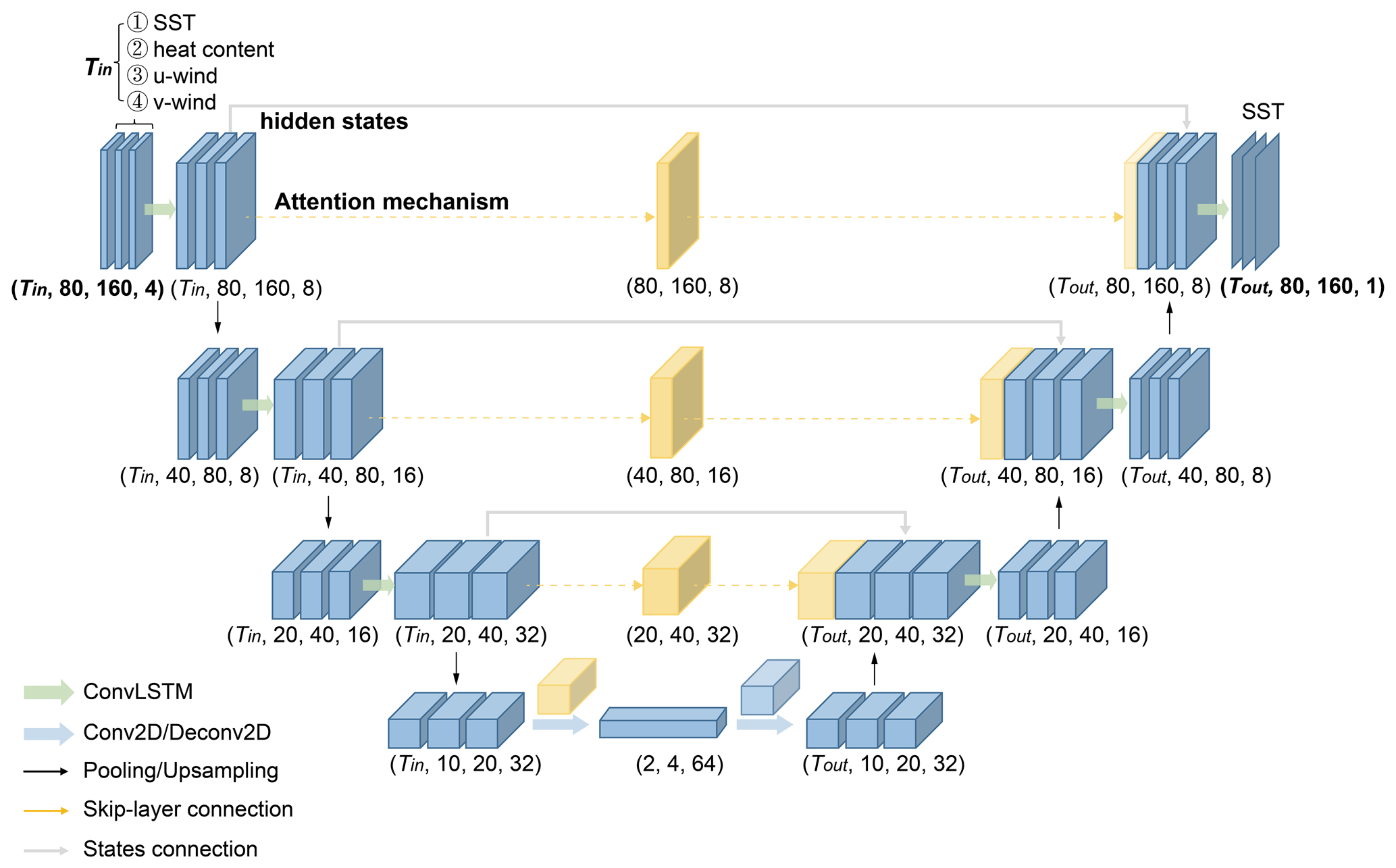
Figure 1The encoder–decoder architecture of ENSO-MC for SST pattern sequence prediction. The encoder contains three ConvLSTM layers and each layer is followed by a pooling layer, and the last layer is a convolutional layer, which allows extracting spatial and temporal features. The decoder comprises one deconvolutional layer, three ConvLSTM layers and three upsampling layers that restore the features to the same size as the initial spatial dimensions (80 × 160). The model uses a skip-layer connection with an attention mechanism and a states connection between the encoder and the decoder to improve forecasting skills. The input variables are the SST, heat content, zonal wind and meridional wind for Tin consecutive months over 40∘ N–40∘ S, 120∘ E–80∘ W (80 × 160, 1∘ × 1∘ resolution), and each type of variable is input to the model as a channel. The output of the model is an SST pattern sequence for the next Tout months.
In order to preserve oceanic processes information for a long time for ENSO forecast, we add skip-layer connection and states connection between the encoder and the decoder on different spatial scales. For each ConvLSTM layer in the encoder, the feature maps of all time steps are fused into one feature map and the weight of each time step is automatically determined through the attention mechanism. These fused feature maps are attached to the corresponding ConvLSTM layers in the decoder to achieve skip-layer connection. Furthermore, in the states connection, the hidden states output by the ConvLSTM layers in the encoder are reserved for the corresponding layer when the decoder is initialized.
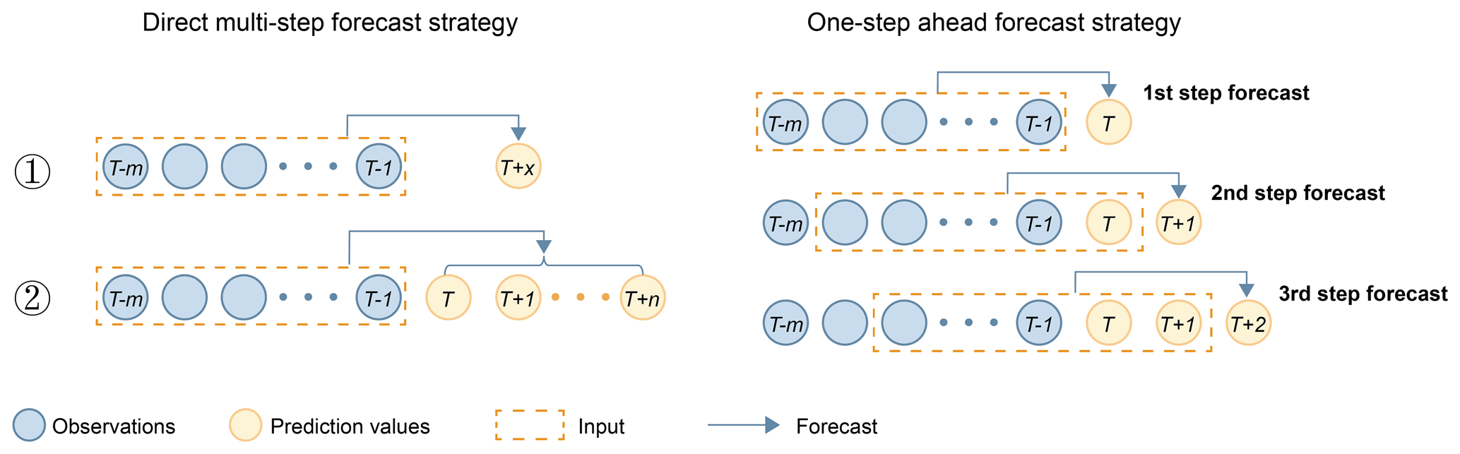
Figure 2Two main strategies of multistep forecasting for ENSO prediction: direct multistep forecast strategy and one-step-ahead forecast strategy. The direct multistep forecast strategy has two methods, the second of which is used in this paper.
In addition, ENSO prediction requires a multiple-step forecasting strategy to achieve long-term prediction. There are two main strategies, direct multistep forecast and one-step-ahead forecast. As shown in Fig. 2, the inputs for direct multistep forecast are fixed observations . To achieve multistep prediction, one of the methods is to build a separate model GT+x for each prediction time step T+x. In the case of predicting SST for the next n months, n models need to be constructed. This is also the strategy used in the paper by Ham et al. (2019), which produced skilful prediction results 1.5 years in advance. Another approach is to build a model that can forecast the entire prediction sequence in a one-shot manner to achieve direct multistep forecasting, which has the advantage of significantly reducing computational and maintenance costs, while a one-step-ahead forecast strategy refers to the multiple use of a one-step model, in which the prediction of the previous time step is used as the input for the prediction of the next time step, i.e., a recursive multistep forecast. In general, one-step-ahead forecasting models are more stable and easier to train (Shi and Yeung, 2018). However, because predictions are used instead of observations, the one-step-ahead strategy allows prediction errors to accumulate, resulting in a rapid decline in performance as the prediction time increases, while direct multistep forecasting has more accurate results in long-term prediction (Taieb et al., 2012). In this paper, a direct multistep forecast strategy and a one-step forecast strategy are both used for prediction and comparison. Considering the computational cost, we use the second direct forecast method instead of the first method of constructing several individual models.
2.2 Selection of physical variables
Using deep neural networks for ENSO simulation is essentially a data-driven method (Reichstein et al., 2019) that is good at mining complicated relations hidden in multidimensional observations of the climate system. Therefore, in addition to building a suitable network to fit the data well, it is important to choose appropriate predictors that well represent ENSO physical processes to train the model (Reichstein et al., 2019).
First, SST is selected as one of the predictors since it is a source of ENSO predictability and a direct reflection of the occurrence of an ENSO event. As the slow-evolving thermal anomaly in the subsurface ocean that provides a key long-lasting memory for ENSO prediction (e.g., Zhang and Levitus, 1997; Tang et al., 2018), we then choose heat content (vertically averaged oceanic temperature in the upper 300 m) as the second attribute, which is closely related to the recharge–discharge oscillator point of view (Jin, 1997a, b; Meinen and McPhaden, 2000; McPhaden, 2003). Third, the westerly wind burst is believed to be an important trigger for El Niño events (Gebbie et al., 2007; Hu et al., 2014; Menkes et al., 2014; Chen et al., 2015; Fedorov et al., 2015) and the atmospheric noise from the wind can be a limit for ENSO predictability (Latif et al., 1988; Moore and Kleeman, 1999). We therefore select SST, heat content and wind stress, in accordance with Bjerknes feedback, to simulate the air–sea interactions responsible for ENSO.
We utilize a Simple Ocean Data Assimilation (SODA) reanalysis data set consisting of sea surface temperature, heat content and wind stress gridded variables from 1871 to 2008 to train the ENSO-MC model, with the resolution 1∘ × 1∘. The domain over 40∘ N–40∘ S, 120∘ E–80∘ W is utilized. To avoid possible overfitting, the data set is divided into a training set and a validation set according to the ratio of 4 to 1. Then we test the performance of the model using the NCEP Global Ocean Data Assimilation System (GODAS) and ERA-Interim data (2010–2019), from which we remove the data that are already in the training set (1981–2008), and there is a 1-year gap between the training set and the test set to reduce the possible influence of oceanic memory.
2.3 Loss function
In our experiments, we combine the losses based on mean squared error (MSE), structural similarity index (SSIM) (Wang et al., 2002) and gradient difference loss (GDL) (Mathieu et al., 2015):
where denotes the observed (predicted) SST pattern sequence and λ represents the weight of each loss. Specifically, MSE measures the discrepancy of each pixel in the sea surface temperature field:
where T represents the length of the prediction sequence. In addition to quantifying the difference in each corresponding pixel value between the observations and predictions, we introduce a loss based on SSIM to measure the global structural differences. SSIM is widely used as a metric to measure the similarity of two images by extracting structural information. It takes into account three features: luminance (l), contrast (c) and structure (s), and its metric formula is the product of these three elements:
where μ is the mean value of a field (luminance), σ is the standard deviation (contrast) and σxy is the covariance of the two fields (structure). C1, C2 and C3 are constants used to maintain the calculations stable. ENSO is associated with the interannual variations of SST anomalies in the tropical Pacific, and the Niño 3.4 index is one of the most commonly used ENSO indicators, which is the average SST anomalies in the equatorial Pacific subregion where the maximum variance of SST is located. Therefore, the SSIM metric can help evaluate important signals embedded in the SST patterns for ENSO prediction (Mo et al., 2014). The range of SSIM is from 0 to 1, and when two fields are the same, the value of SSIM is 1. Therefore, we construct the SSIM-based loss function as
We also consider gradient information in the loss functions. The SST gradient represents the difference in the sea surface temperature across the adjacent area. Previous studies have shown that MSE loss function tends to average the values of all points in the whole prediction field to minimize the MSE error, while considering the gradient difference value can alleviate this problem (Oprea et al., 2020). Besides, the SST gradient also plays a role in the atmospheric circulation. The region with a large SST gradient will generate stronger winds, which in turn will promote the further increase of the SST gradient (Bjerknes, 1969). As ENSO approaches maturity, the SST gradient increases gradually. Therefore, we use the GDL to measure the gradient difference of the sea surface temperature field:
where i,j denote the pixel position on the sea surface temperature field. Here we only consider the gradient difference in neighbouring regions. In future studies, we will consider the gradient difference at a larger spatial scale according to the characteristics of ENSO, such as the difference in SST between the western Pacific and the central Pacific during ENSO (Zinke et al., 2021).
3.1 Influence of the input sequence length
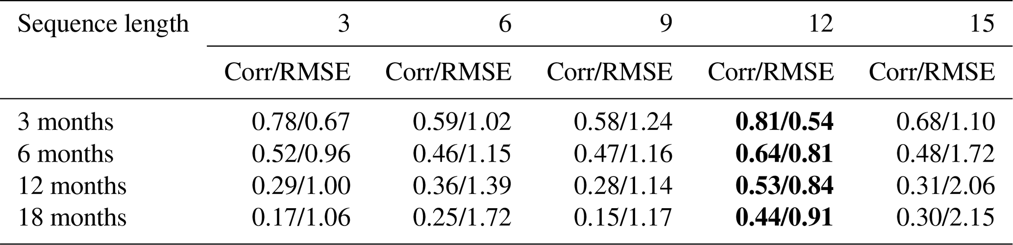
Appropriate input sequence length is critical for ENSO prediction of the multichannel model. We use data from the past 3, 6, 9, 12 and 15 months as inputs to predict the development of ENSO in the next 18 months to examine the effects of different input sequence lengths on ENSO predictions. Table 1 shows the comparison of correlation skill and RMSE of lead times. For the correlation coefficient, the higher the value is, the higher the forecasting skill is, and the smaller RMSE represents the higher skill. The results show that the ENSO-MC model performs best with data from the past 12 months as input. This may be because the variables we select have long-term memory for the development of ENSO, such as oceanic heat content. A longer input sequence contains more information that is helpful to ENSO prediction, but also contains more noise that interferes with the prediction, so the improvement of forecasting skill is not positively correlated with the increase of input sequence length. But for different models and forecasting horizons, the most appropriate input sequence lengths may not be the same.
Table 1Correlation skill (Corr) and root mean square error (RMSE) of lead times with different input sequence lengths. Bold values are the best of the five input sequence lengths.
3.2 Physical variable sensitivity for the multichannel structure
With the physical variables we selected in Sect. 2, we construct multichannel input that takes into account the complicated spatiotemporal interactions in the ocean and atmosphere underpinning the onset and development of ENSO events. For the grid observations of monthly SST, heat content, zonal wind and meridional wind, we treat each type of input variable as a channel in the first ConvLSTM layer, and thus there are four channels. The number of channels is the depth of the matrices involved in the convolutions, so that the cross-correlation and transmission between these ocean–atmosphere data can be calculated in the convolution operation. We design an ablation experiment to examine the contribution of predictors and the effectiveness of the multichannel structure. In addition to SST, the most important predictor, we remove heat content (t300) and wind from the respective inputs to detect their effects on the correlation skill of the Niño 3.4 index. As shown in Fig. 3, the model using the three key ingredients of Bjerknes feedback (SST, heat content and wind) as input produces more favourable forecast skill than the ones that remove one of them, which indicates that the multichannel structure can help to learn the ocean–atmosphere coupling between several important predictors. For the models with two predictors, the model containing the wind predictor shows slightly higher forecasting skill in the first few months, while the one containing the heat content predictor performs more stable skill at lead times of more than 8 months. It suggests that the memory of subsurface heat plays an important role in ENSO prediction on seasonal to interannual time scales, which is consistent with previous research.
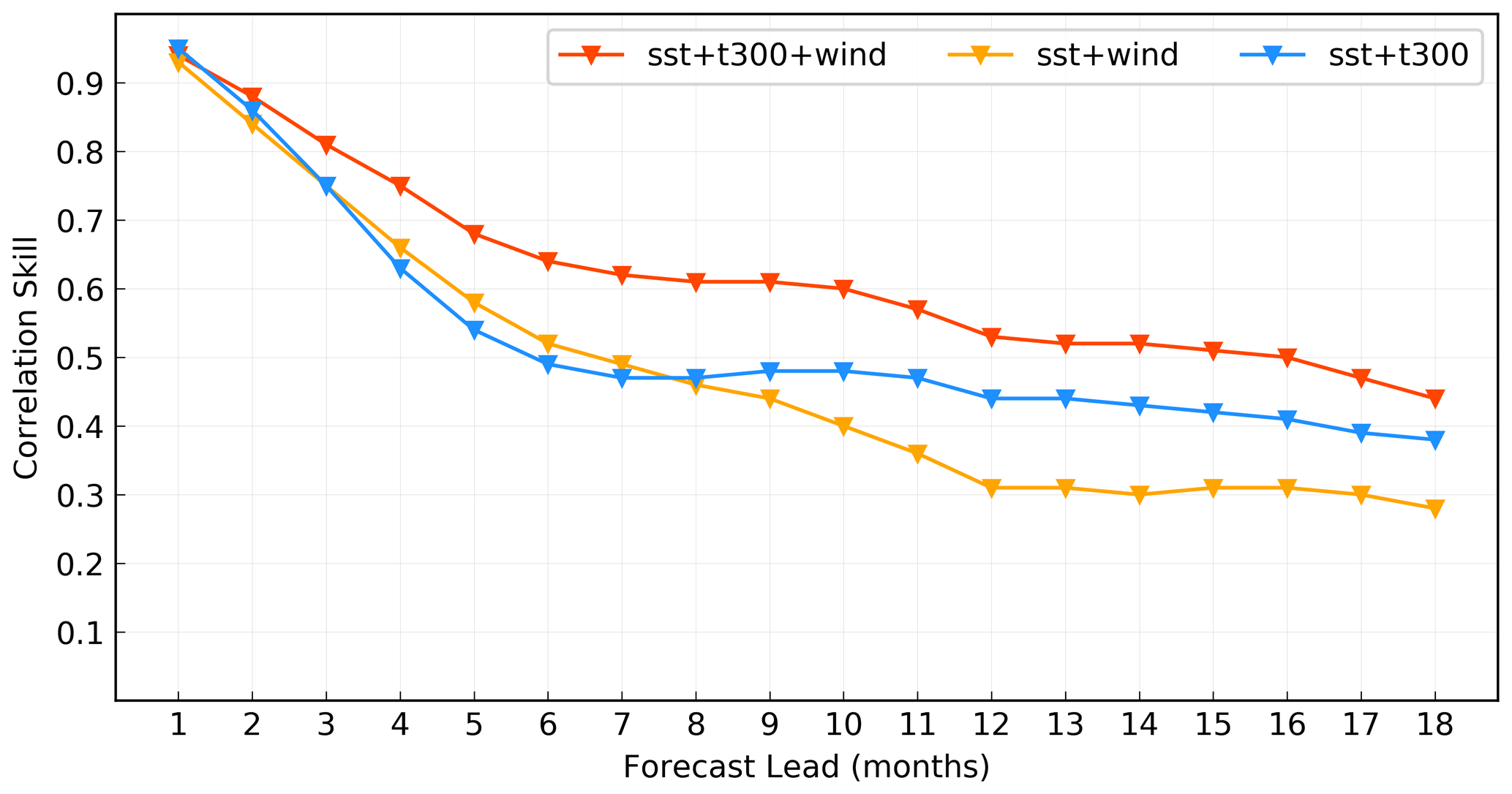
Figure 3The correlation skill of the Niño 3.4 index of the ENSO-MC model with different predictors.
3.3 Effectiveness of the model components
The ENSO-MC model learns the features of ENSO at different spatial scales with the convolution and max-pooling layers in the encoder, and gradually restores the spatial dimensionality of the original SST field in the decoder. With symmetrical structural design of the encoder and decoder as shown in Fig. 1, skip-layer connection is used to transfer features form the encoder to the decoder to recover spatial information lost during downsampling (dashed yellow line in Fig. 1). Rather than transferring the original features of all time steps obtained from the encoder, we design an attention mechanism to enable the skip-layer connection to automatically learn the attention weights on the temporal sequence because these air–sea features may have different effects on ENSO development at different time scales. As shown in Fig. 4i, the encoder obtains the features after max-pooling and convolution calculation at the nth layer. Using a two-layer densely connected neural network, we obtain the attention weight of each time step’s features according to Eq. (6), where are reshaped from fn:
where Wαf, Wβα are weight matrices created by the layer, and bαf, bβα are the bias vectors. β represents the contribution of each time step to prediction. According to Eq. (7), the feature maps of each time step are multiplied by the corresponding weights, and the fused maps are obtained by adding them along the time dimension:
where are the feature maps to be transmitted in the skip-layer connection, which are connected to the features of the corresponding layer in the decoder. We also add states connection between the encoder and the decoder (grey line in Fig. 1), where the hidden states output by the ConvLSTM layers in the encoder are reserved for the corresponding layer when the decoder is initialized. With the methods of skip-layer connection and states connection, the model can make full use of the information extracted from the encoder before ENSO events, which help stabilize training and convergence.
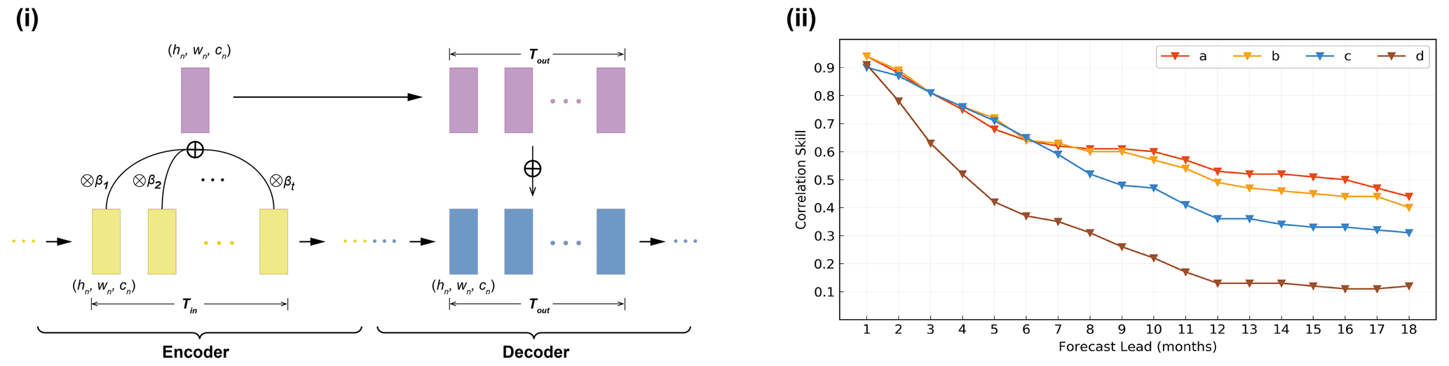
Figure 4(i) The detailed structure of the skip-layer connection and attention mechanism between the encoder and decoder at the nth layer in ENSO-MC. (ii) The correlation skill of the Niño 3.4 index of the forecast lead month in models with different structures: (a) ENSO-MC model of skip-layer connection with attention mechanism and states connection, (b) ENSO-MC model without attention mechanism, (c) ENSO-MC model without states connection and (d) ENSO-MC model without skip-layer connection.
We remove the attention mechanism (model b), states connection structure (model c) and skip-layer connection structure (model d), respectively, from the constructed ENSO-MC model (model a) to analyse their effects on model performance. As shown in Fig. 4ii, the two connection structures, especially the skip-layer connection structure, have a great influence on the prediction results. In model b, we use average weights to replace the attention mechanism. Compared with model a, the self-attention mechanism can play a greater role in long-term ENSO prediction.
3.4 Effects of different loss functions
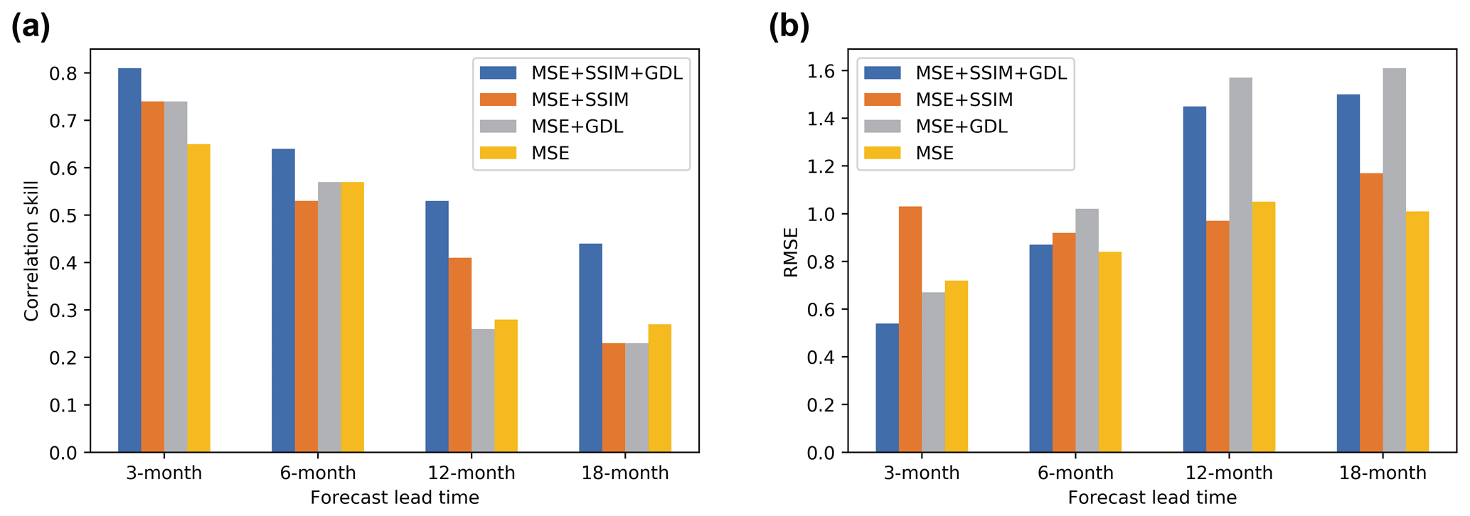
In order to balance the optimization speed of each loss in the training process, we set λmse=7, λssim=9 and λgdl=1. The effectiveness of combined loss function is validated. As shown in Fig. 5a, although SSIM and GDL do not significantly improve the model performance when combined with MSE alone, the combination of MSE, SSIM and GDL loss functions achieve the best performance on the correlation skill. Moreover, since GDL loss function tends to retain extreme values and MSE loss function tends to smooth all values, the presence of GDL inhibits the decrease of MSE, so the MSE errors of the models with GDL loss function are higher than the ones without GDL (Fig. 5b). In addition, comparing the results of correlation skill and RMSE in Fig. 5a and b, low RMSE values do not represent high correlation skills. Therefore, it is necessary to explore loss functions suitable for ENSO prediction other than MSE to balance the training of the model.
4.1 Simulation of the two types of ENSO
The simulation ability of ENSO-MC for different types of events is evaluated in this section. We first select the typical EP El Niño, CP El Niño and La Niña events in recent years to validate the forecast skills on individual events in detail. The forecasts of spatial patterns and Niño 3.4 index time series are compared with observations. Besides, the correlation skills for all targeted seasons of the model are further validated.
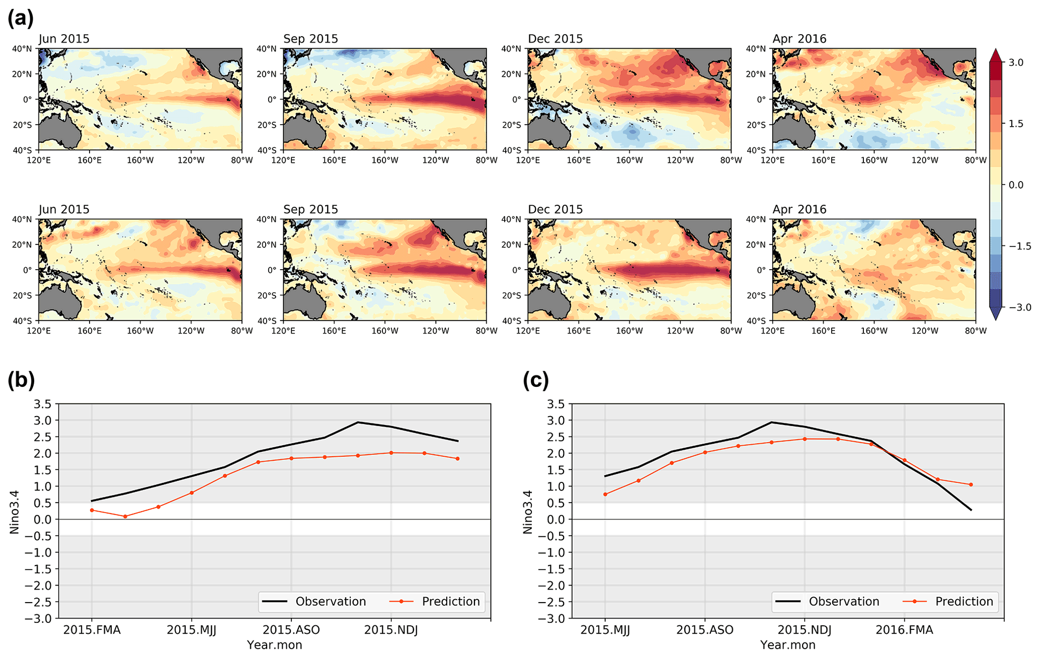
Figure 6The SST anomalies patterns and index prediction results for 2015–2016 El Niño using ENSO-MC. (a) Spatial development of SST anomalies predicted (the first row) 1 year in advance compared with the real observations (the second row) for the onset, growth, mature and decay phases. (b) Niño 3.4 index time series forecast initiated in the FMA season using ENSO-MC (red line) and the observed Niño 3.4 index (black line). (c) Niño 3.4 index time series forecast initiated in the MJJ season using ENSO-MC (red line) and the observed Niño 3.4 index (black line).
We validate the performance of ENSO-MC for simulating the latest extreme El Niño event in 2015–2016. It can be classified as an EP-type event, and some studies have suggested that the 2015–2016 El Niño event appears to have been a mixture of EP and CP patterns (Santoso et al., 2017). Figure 6a compares the predicted spatial evolution of SST anomalies for the 2015–2016 event (the first row) 1 year in advance and the corresponding observed patterns (the second row). The 4 months shown in the Fig. 6a (June, September, December and April) represent the main states involved in the phases of ENSO evolution. The temperature anomalies emerge in the eastern equatorial Pacific (June 2015), which are then amplified and spread to the central equatorial Pacific (September 2015). When the event reaches the mature stage (December 2015), the centre of the anomalies tends to move toward the central equatorial Pacific, eventually decaying in April 2016. The prediction of SST anomalies development in the equatorial Pacific is in reasonable agreement with the observation results. But in the subtropics, there is a strong warm bias in the northeastern Pacific during the mature and decay stages, and in the South Pacific, there is more cooling in the model than observed. According to the predicted SST anomalies patterns, the time series of the Niño 3.4 index is further calculated (Fig. 6b, c). The amplitude and temporal evolution of the 2015–2016 El Niño for the 1-year-lead forecast of ENSO-MC are almost consistent with observations, although with weaker amplitude compared with the observed Niño 3.4 index. In addition, the forecasts initiated during the May–June–July (MJJ) season (Fig. 6c) agree a bit more favourably with the observations than those initiated during February–March–April (FMA) 2015 (Fig. 6b).
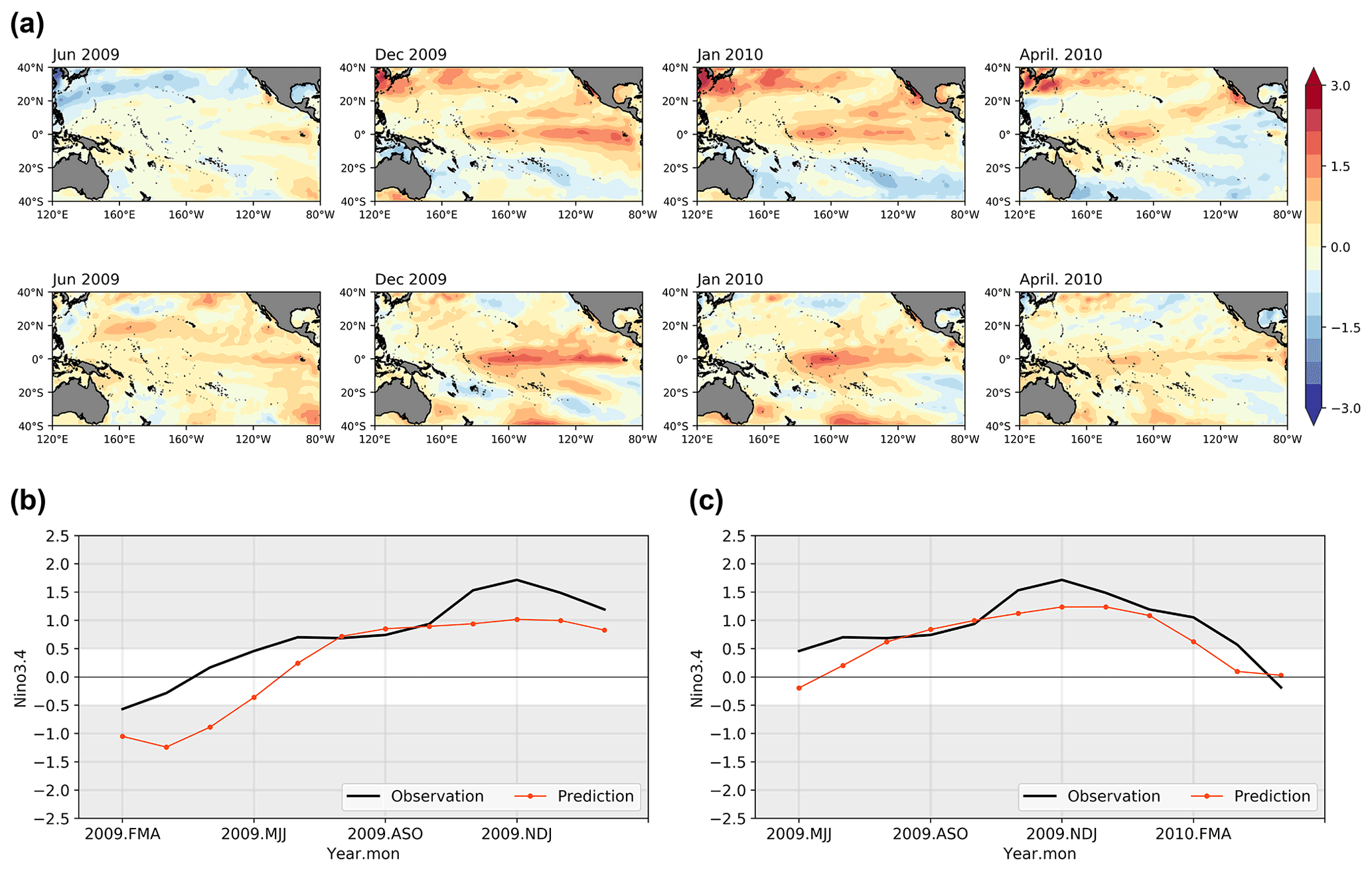
Figure 7The SST anomalies patterns and index prediction results for 2009–2010 El Niño using ENSO-MC. (a) Spatial development of SST anomalies predicted (the first row) 1 year in advance compared with the real observations (the second row) for the onset, growth, mature and decay phases. (b) Niño 3.4 index time series forecast initiated in the FMA season using ENSO-MC (red line) and the observed Niño 3.4 index (black line). (c) Niño 3.4 index time series forecast initiated in the MJJ season using ENSO-MC (red line) and the observed Niño 3.4 index (black line).
By contrast, the prediction results of the 2009–2010 event, which is known as a CP El Niño, are shown in Fig. 7. The spatial patterns of the SST anomalies predicted (the first row) and observed (the second row) are shown in Fig. 7a. The observations show a pronounced central Pacific warming. Specifically, the SST anomalies appear (June 2009), grow (December 2009) and reach maturity (January 2010) in the central Pacific, whose meridional shift on the Equator is less obvious. The model captures most of these features, although the anomalies distributed over the central equatorial Pacific are smaller in amplitude and scope than observed during the growth and mature phase, and the CP characteristics of ENSO are not as pronounced as the actual ones. There is also some evident bias in the mid-latitudes. For the Niño 3.4 index results (Fig. 7b, c), the ENSO-MC model exhibits a similar trend but weaker amplitude compared with the observed values. Especially when initiated in FMA 2009 (Fig. 7b), the model tends to underestimate the strength during the growth phase.
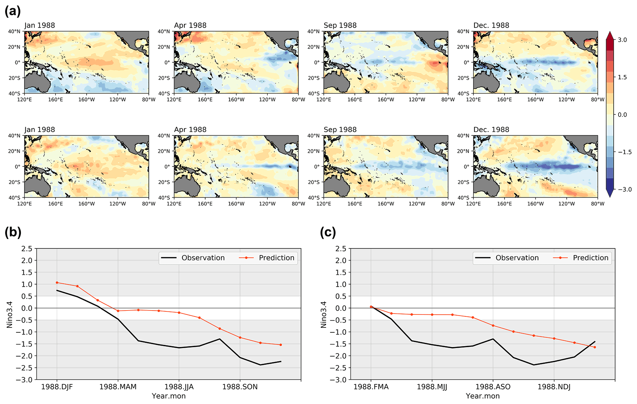
Figure 8The SST anomalies patterns and index prediction results for 1988–1989 La Niña using ENSO-MC. (a) Spatial development of SST anomalies predicted (the first row) 1 year in advance compared with the real observations (the second row) for the transition, onset, growth and mature phases. (b) Niño 3.4 index time series forecast initiated in the DJF season using ENSO-MC (red line) and the observed Niño 3.4 index (black line). (c) Niño 3.4 index time series forecast initiated in the FMA season using ENSO-MC (red line) and the observed Niño 3.4 index (black line).
Table 2Correlation skill (Corr) and root mean square error (RMSE) of lead times with different input sequence lengths.
Given the different mechanisms and periods of warm El Niño and cold La Niña events, we also evaluate the simulation ability of the model for a La Nina event. Figure 8 shows the prediction results for 1988–1989 strong La Niña. The simulated evolution of SST anomalies spatial structure along the Equator are in reasonable agreement with observations (Fig. 8a). The cold temperature anomalies occur in the eastern Pacific, then spread to the central Pacific and reach maturity. However, the predicted cold anomalies are weaker in amplitude and do not extend as broad in area as observed. It is evident in the Niño 3.4 index time series results, where the amplitudes of the predictions are weaker than the observed values regardless of whether the initialization is performed before the event (Fig. 8b) or in the early stage of its development (Fig. 8c).
In addition to the above three typical events in recent years, the prediction results of other events that occurred between 1984 and 2019 are detected. For each event, we compare the spatial development of predicted and observed SST anomalies in the equatorial Pacific from the onset to the maturity stage.
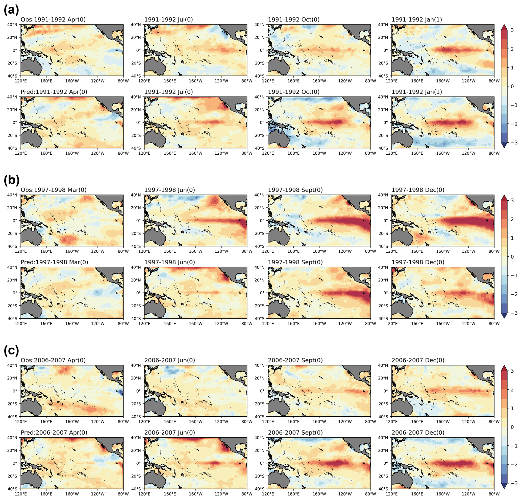
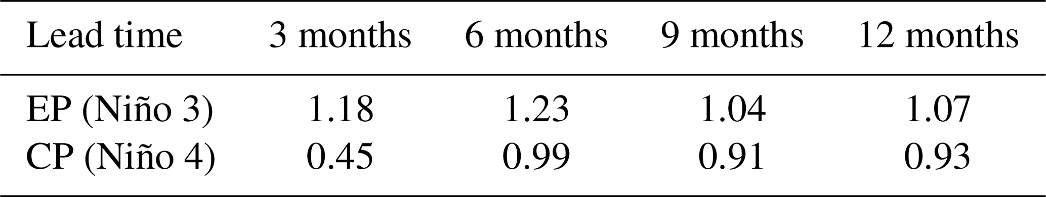
Figure 9SST anomalies of three EP El Niño events in (a) 1991–1992, (b) 1997–1998 and (c) 2006–2007 from the onset to the maturity stage, with observations in the first row and predictions in the second row for each event. The mature phases here are the months when the El Niño events peak. The “0” and “1” next to the calendar month denote the year when the El Niño event occurred and the following year respectively.
Figure 9 shows the simulation results of the ENSO-MC model for three EP El Niño events of 1991–1992, 1997–1998 and 2006–2007, with observations in the first row and predictions in the second row for each group. The results show that the model can simulate the occurrence and development of SST anomalies for each event. However, for some events with less significant EP-type characteristics (for example, that of 1991–1992), the SST anomalies centre of predictions is closer to the central Pacific than observed. In addition, for some super-strong events (for example, that of 1997–1998) and weak events (for example, that of 2006–2007), the amplitude of the predicted results at the mature phase may be lower or higher than observed.
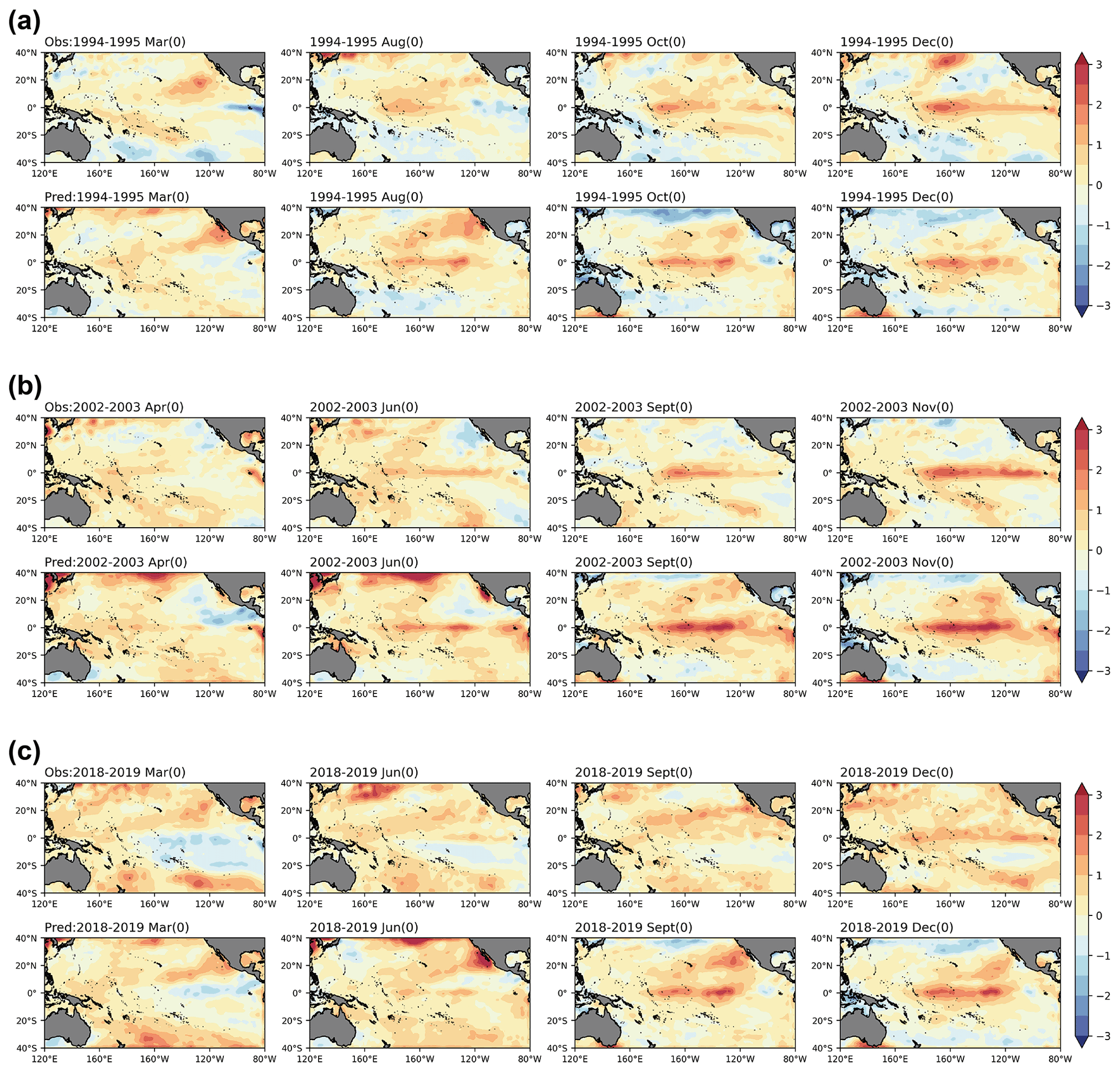
Figure 10The same as in Fig. 9, but for the three CP El Niño events in (a) 1994–1995, (b) 2002–2003 and (c) 2018–2019.
The prediction results for three CP El Niño events in 1994–1995, 2002–2003 and 2018–2019 are displayed in Fig. 10. For the events of 1994–1995 and 2018–2019, the model can simulate the process that the SST anomalies in the northeast Pacific propagate to the southwest and finally contribute to the occurrence of CP events. The amplitude and centre location of the predicted anomalies are also in agreement with the observations. However, the meridional distribution of predicted SST anomalies is not as broad as observed in the mature stage. The observed SST anomalies extends eastward to 80∘ W, while the predicted value extends roughly between 100 and 120∘ W.
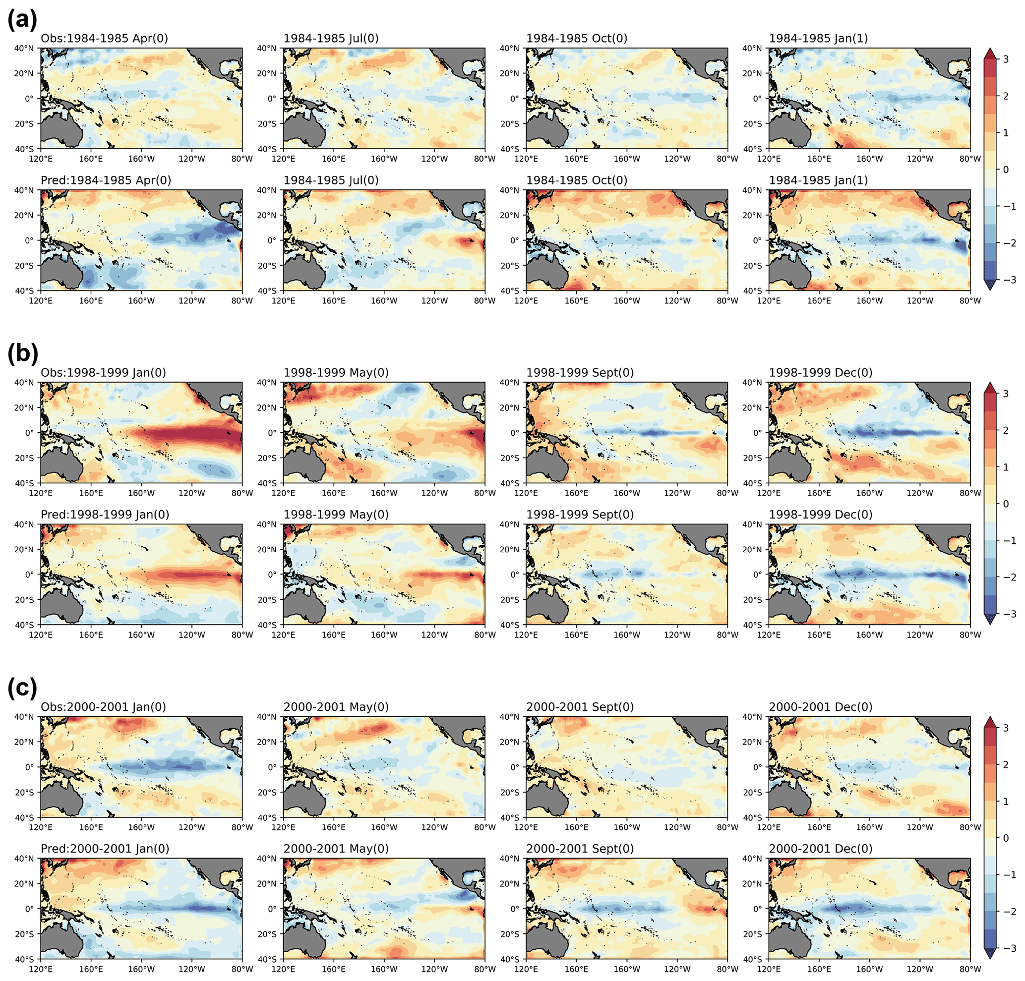
Figure 11The same as in Fig. 9, but for the three CP El Niño events in (a) 1994–1995, (b) 2002–2003 and (c) 2018–2019.
Figure 11 shows the predictions of three La Niña events in 1984–1985, 1998–1999 and 2000–2001. These three events occurred under different conditions. The events of 1984–1985 and 1998–1999 were preceded by strong El Niño events, and the 1998–1999 event occurred more rapidly. The 2000–2001 La Niña was another weaker event after the previous La Niña event had ended. Compared with observations, the model can simulate the occurrence, development and phase transition or persistence of La Niña events.
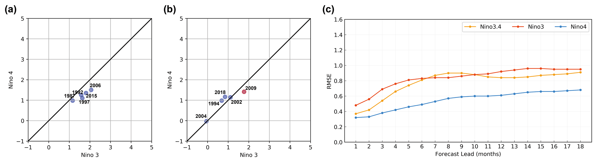
Figure 12Scatterplots in Niño 3–Niño 4 index plane of 12-month-lead predictions for all (a) EP El Niño events and (b) CP El Niño events during the peak phase from 1984 to 2019. (c) Root mean square error (RMSE) of the Niño 3.4, Niño 3 and Niño 4 indexes between the forecast results of the ENSO-MC model and observations during the validation period.
In addition to comparing the detailed spatial distribution of SST anomalies, the related indexes and metrics are calculated to further evaluate the simulation performance of the ENSO-MC model. The Niño 3 index (average SST anomalies over 5∘ N–5∘ S, 150–90∘ W) and the Niño 4 index (average SST anomalies over 5∘ N–5∘ S, 160∘ E–150∘ W) are commonly used to define two types of El Niño events. Events with a Niño 4 index greater than that of Niño 3 are regarded as CP El Niños, and events with a Niño 3 index greater than that of Niño 4 are classified as EP El Niños. Figure 12a, b shows the distribution for Niño 3 and Niño 4 indexes calculated from the model's 1-year-lead predictions of the peak periods for all EP events (Fig. 12a) and CP events (Fig. 12b) from 1984 to 2019. The results show that the model can correctly classify five EP events (1987–1988, 1991–1992, 1997–1998, 2006–2007 and 2015–2016) and three CP events (1994–1995, 2002–2003 and 2018–2019) in the past 30 years, but misjudge the event of 2009–2010 as the EP type and indicate that no El Niño event occurred in 2004 (Niño 3 = 0, Niño 4 = 0). The CP event of 2004–2005 is much weaker than other CP ones, making it more difficult for the model to capture its development. We also make statistics on the RMSE between the predictions and official records of the Niño 3 and Niño 4 indexes for all EP/CP El Niño events at the mature phase (Table 2) and for the whole validation period (Fig. 12c), and find that although the model has a higher classification accuracy for EP events, the index error of predictions for EP events is larger than that for CP. It may be because most of the strong El Niños are EP-type events, and the prediction skills of the model for such extreme events need to be improved. The SST anomalies distribution in Fig. 9 also shows that for some EP events, there is a difference in amplitude between predictions and observations for the maturity stage of the event, while that of the CP events is consistent with the observations (Fig. 10).
4.2 Correlation skills for different calendar months
The model also shows a reasonable forecast of ENSO 1 year in advance for all targeted seasons (Fig. 13). Figure 13a shows the correlation skill of Niño 3.4 index forecasts for the GODAS validation data from 1982 to 2019, which are initiated in each calendar month and predicted for a lead of up to 18 months. The correlation skill in the model is above 0.5 for a lead of 11 months. Figure 13c shows the results for the past decade whose validating period is from 2010 to 2019. The results in Fig. 13c perform only slightly more skilfully than those in Fig. 13a, indicating the robustness of the model in terms of validation time. We also compare the two forecast strategies in deep learning, that is, the one-step-ahead forecast strategy and the multistep forecast strategy. Figure 13a and c are the results of multistep prediction, while Figs. 13b (1982–2019) and 5d (2010–2019) are the results of one-step prediction. It shows that regardless of the season from which the forecast is started, the skills would be reduced for predictions targeting the late boreal spring (April–May–June, AMJ), as indicated by the black numbers in Fig. 13. We also calculate the overall decline of forecasting skills in each target month compared with the previous month and the results are presented in Fig. 14. The prediction skills of the model decline most from April to May, regardless of whether the multistep or one-step-ahead forecast strategy is used. Besides, Fig. 14 shows that the performance of the model is slightly improved in winter, which leads to the improvement of skills after 12 months in Fig. 13. Since the seasonal variation of SST anomaly variance is weaker in spring, it is difficult for the model to capture useful information, which leads to the spring predictability barrier (SPB), while the strong signals of ENSO during winter are more easily learned by the model. In addition, the one-step-ahead strategy has a larger decline after the boreal spring (Fig. 14), and the subsequent forecasts are more susceptible to the SPB due to its cumulative error (Fig. 13b, d), while the method of the multistep strategy can reduce the influence (Fig. 13a, c). We can conclude that the ENSO-MC model using the multistep forecast strategy is less affected by spring predictability barriers.
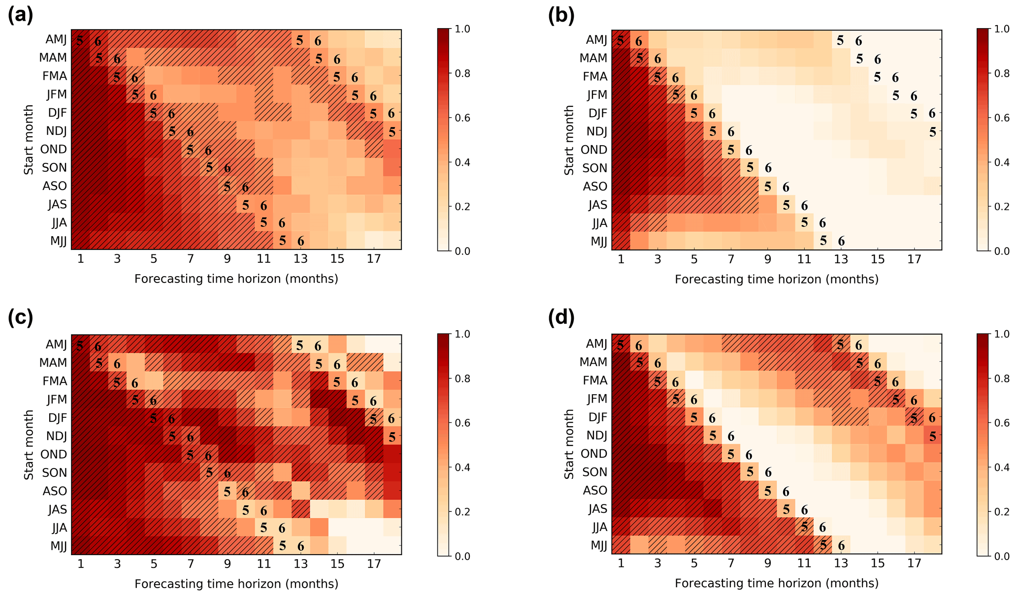
Figure 13The correlation skills of the Niño 3.4 index forecasts started from each calendar month in ENSO-MC using the multistep forecast strategy (a) and the one-step-ahead forecast strategy (b) for the GODAS data from 1982 to 2019. Panel (c) is the same as (a), except for the GODAS data from 2010 to 2019. Panel (b) is the same as (d), except for the GODAS data from 2010 to 2019. Hatches represent the forecasts with correlation skill exceeding 0.5, and the black numbers mean the target forecast months.
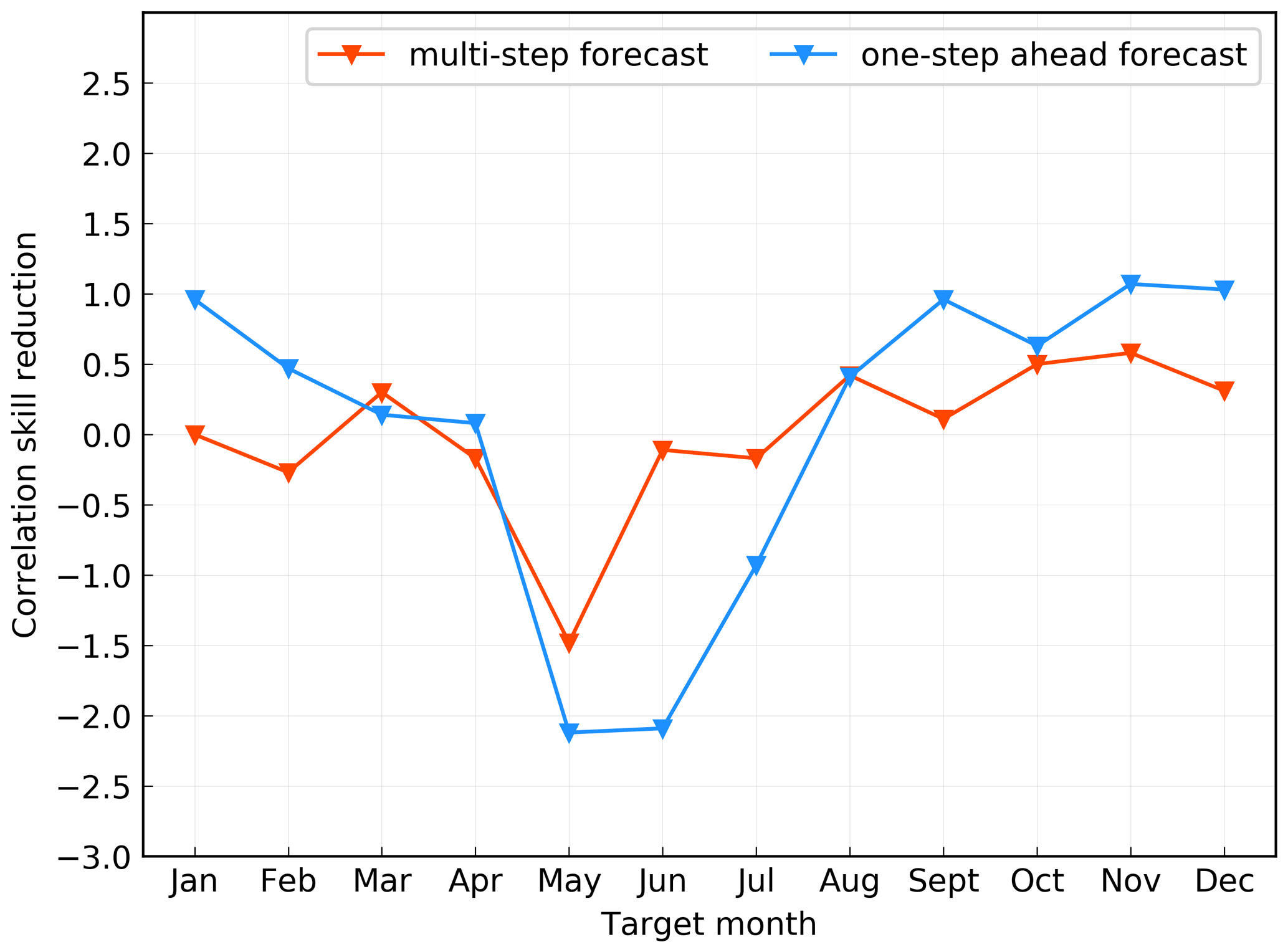
Figure 14The decline of forecasting skills for ENSO in each target month using the multistep forecast strategy and the one-step-ahead forecast strategy.
It should be noted that the correlation coefficient skills of the Niño 3.4 index obtained by simulating the SST anomalies spatial distribution are not as high as those obtained by using the deep neural network to predict the Niño 3.4 index directly, such as the results of Ham et al. (2019). This is because the former has a higher prediction target dimension, and the cumulative error of each point of the spatial field is larger than the error of direct prediction of a single index. This is also one of the key issues to be solved in the future development of the ENSO-MC model.
Based on the ENSO-MC model which successfully simulates different types of ENSO events, we can further explore the ENSO dynamics learned by the ENSO-MC model and observe the signals before the onset of events. In addition, since the ENSO-MC model using the multistep forecast strategy achieves better performance than using one-step strategy, here we calculate the saliency maps based on the multistep forecasting model for precursor analysis and sensitive area identification. Considering the important role of subsurface thermal memories in ENSO prediction, the precursory characteristics in heat content of different types of events are discussed here. We select five EP El Niño events (1987–1988, 1991–1992, 1997–1998, 2006–2007 and 2015–2016), three CP El Niño events (1994–1995, 2002–2003 and 2009–2010) and three La Niña events (1988–1989, 2007–2008 and 2010–2011) which occurred in the past 30 years, and calculate the precursor maps of the heat content anomaly in the year prior to each event.
Specifically, the precursor maps of each event are obtained by computing the gradient of the regressed output with respect to the input with the saliency map method. The maps tell us how the output value will change when the pixel at this position in the input image changes slightly, that is, the sensitivity of the predicted results to the perturbations in each region. In this way, we can get the initial perturbation distribution that would develop into an ENSO event. The gradient calculation is equivalent to the process of seeking the gradient of the errors with respect to the weights during training a machine learning model, which represents the contribution of each weight to the total loss. We calculate the deviations between the output and the real situation Y, fix the weights of the ENSO-MC model and perform back propagation for each pixel (x,y) in the input H at each moment τ:
Then we obtain a series of heat maps over the heat content predictors . Each Mτ indicates the perturbation sensitivity distribution in heat content Hτ for τ-lead time. For each event, 12 heat maps are obtained, which describe the precursor development in the year preceding the event. We add up the maps of τ-lead time of each event for one type to obtain the composite evolution maps for each type. For example, the composite precursor map of τ-month lead for the EP-type El Niño is obtained by adding up the precursor maps of τ-lead time for all five EP events. The composite maps of the CP-type El Niño and La Niña are obtained in the same way. The precursor maps from 12-month lead to 1-month lead of the EP-type El Niño, CP-type El Niño and La Niña are shown in Fig. 15, and we present results every few months for each type to see more clearly how precursors change over time. Since the composite maps are the sum of the saliency maps of each event, here we focus on the distribution of perturbation without considering the intensity, and the saliency values in Fig. 15 are the standardized results of the scale between 0 and 1. For EP El Niño (Fig. 15a), the subsurface temperature component presents large anomalies in the equatorial Pacific, especially in the central and western Pacific, the subtropical northeast Pacific and the subtropical South Pacific. With the occurrence of El Niño, the anomalies weaken in the equatorial region and slightly intensify in the subtropical area, and the large anomalies of the precursory perturbation for CP El Niño (Fig. 15b) are concentrated in the subtropical northeast Pacific. As El Niño approaches, the disturbance tends to spread to the southeast. Regarding the subsurface disturbances for La Niña (Fig. 15c), their anomalies are concentrated in equatorial regions and propagate from the western to the eastern Pacific.

Figure 15The composite evolution maps of initial perturbations in heat content before (a) EP-type El Niños, (b) CP-type El Niños and (c) La Niñas from 12-month lead to 1-month lead.
On the whole, the subsurface signals distributed in Fig. 15a are more intense and more extensive than those in Fig. 15b, indicating that the occurrence of the EP-type El Niño is more related to the subsurface dynamics, while the CP events may be more affected by the atmospheric convection. Specifically, compared with Fig. 15b (CP-type El Niño), Fig. 15a (EP-type El Niño) shows a more pronounced signal, especially in the equatorial Pacific. It may be related to the stronger zonal tilt change of the equatorial thermocline and larger eastward movement of convection in the tropical Pacific before the EP-type events.
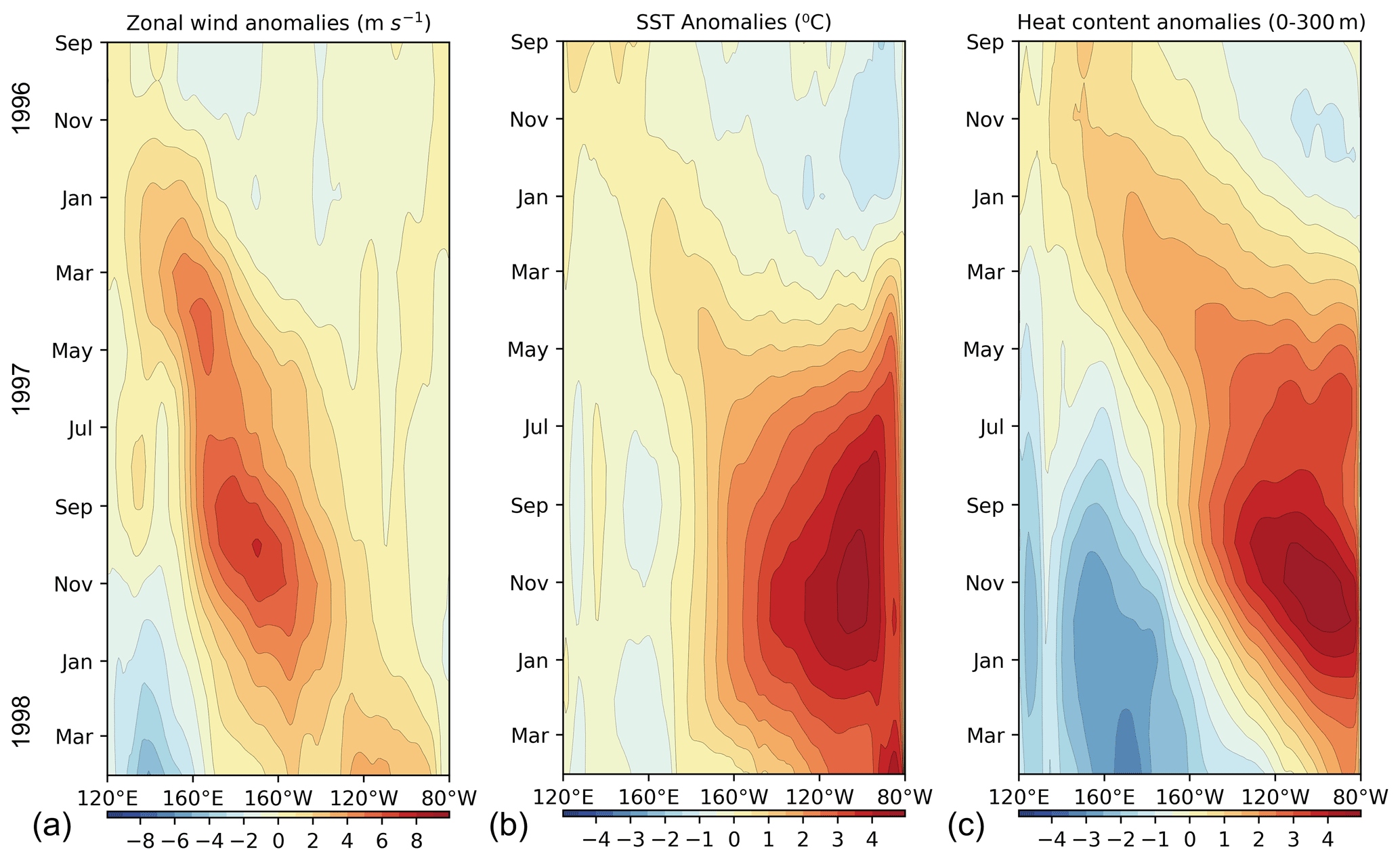
Figure 16Longitude-time diagram of monthly surface zonal wind anomalies (a), SST anomalies (b) and heat content (t300) anomalies (c) across the equatorial Pacific (2∘ N–2∘ S, 120∘ E–80∘ W) from September 1996 to April 1998. Data are based on NCEP Global Ocean Data Assimilation System and ERA-5.
For example, as shown in Fig. 16, a series of westerly wind events along the equatorial Pacific led to an abrupt relaxation and reversal of trade winds in the western and central equatorial Pacific in early 1997. The westerly wind anomalies generated downwelling Kelvin waves, which propagated eastward and deepened the thermocline in the eastern Pacific in late 1997. The depressed thermocline limited the upwelling of subsurface cold water, prompting the development of warm surface temperatures. Meanwhile, westward-propagating Rossby waves shallowed the thermocline in the western Pacific. These processes led to significant changes in the equatorial thermocline (Fig. 15a), a flattening of the thermocline and a decrease in the zonal SST gradient along the Equator. The reduction in the SST gradient in turn further weakened the trade winds, leading to the rapid development of the 1997–1998 El Niño. La Niña events usually occur in the second year after a warm event. As shown in Fig. 15c, there are precursor signals produced by wind forcing propagating eastward from the western tropical Pacific in the subsurface from 12-month lead to the occurrence. Combined with the mechanism of the La Niña event, the signal would shoal the thermocline in the eastern Pacific and enhance the upwelling of cold subsurface waters, thereby ending the El Niño event and triggering a subsequent cold event.
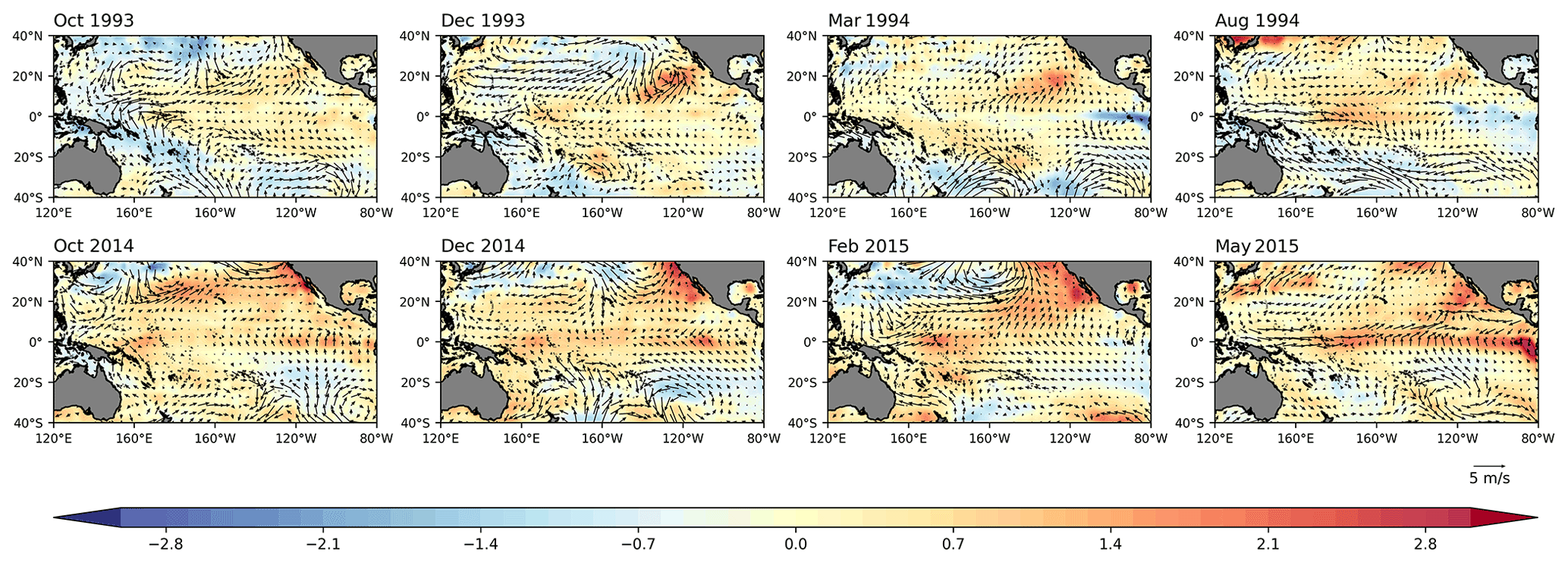
Figure 17The SST and 10 m wind-vector anomalies for the different seasons before the 1994–1995 CP El Niño and 2015–2016 EP El Niño events.
While the equatorial subsurface signal is weak in Fig. 15b, there is an obvious signal in the North Pacific. The results are consistent with the previous studies that the negative phase of the North Pacific Oscillation promotes the development of SST anomalies in the central Pacific (Yu and Kim, 2011). In addition, there are robust signals over the northeastern Pacific in both types of El Niño events (Fig. 15a, b). The distribution is similar to the spatial structure of the Pacific meridional mode (PMM). The PMM is forced by mid-latitude atmospheric variability in the Northern Hemisphere and evolves toward the Equator subsequently, which can affect ENSO. As shown in Fig. 17, 1 year before the 1994–1995 CP El Niño event, there were warm subtropical SST anomalies extending southwest from Baja, California. The SST anomalies weakened the trade winds and reduced the surface evaporation over the region via wind–evaporation–SST (WES) feedback. The reduction in evaporation allowed warm waters to expand further southwestward, enhancing the PMM and eventually reaching the Equator, which weakened equatorial trade winds and triggered an El Niño event in late 1994. The PMM not only appeared before the CP El Niño event, for example, the emergence of PMM in late 2014 contributed to the development of the 2015–2016 El Niño event (Fig. 17). It indicates that signals outside the tropics play an important role in the prediction of El Niño and PMM can be regarded as a precursor to El Niño.
A saliency map shows which input pixels produce the largest increase in output values with minimal change. The idea is similar to the targeted observation strategy, that is, prioritizing the deployment of observations in the sensitive areas where small perturbations tend to have the greatest impacts on the forecasts. The saliency map method is therefore appropriate to identify the sensitive areas of targeted observation for ENSO. The areas with large values in the saliency map indicate that improving the accuracy of observations in these sensitive areas is the most efficient way to correct the output. Here we explore the sensitive areas of the surface and the subsurface layers respectively, so in addition to heat content, the saliency maps of SST are also calculated. Since the sensitive area is a common attribute, it should be universal to all ENSO events; therefore, different types of ENSO are not considered here. We select eight El Niño events (1987–1988, 1991–1992, 1994–1995, 1997–1998, 2002–2003, 2006–2007, 2009–2010 and 2015–2016) and three La Niña events (1988–1989, 2007–2008 and 2010–2011) that occurred in the past 30 years, and calculate the saliency maps of SST and heat content for each event according to the method described in Sect. 4. Then all the saliency maps of SST are added up to obtain the composite saliency map of the surface (Fig. 18a), and that of the subsurface (Fig. 18b) is obtained in the same way. The saliency values in the figure are the standardized results of the scale between 0 and 1. The anomalies of surface disturbance are mainly distributed in the northern central Pacific, the central Pacific and the western Pacific. The anomalies in the North Pacific are more intense than those in the South Pacific. For the subsurface temperature precursory, the perturbation possesses a wide range of anomalies in the equatorial Pacific and the North Pacific, and the anomaly values are more intense than that of surface disturbance. Since ENSO-MC regards multi-variable fields as multiple channels, the saliency regions obtained from the surface layer and the subsurface layer may affect each other. As shown in Fig. 18, the large-value region of surface (a) overlaps with that of subsurface (b); therefore, we first artificially define six common regions with large values (black boxes in the Fig. 18) and perform sensitive experiments on the surface and subsurface respectively. Since the error is random in real observations, we use random perturbations for sensitivity experiments. For each of the 11 selected ENSO events, 30 sets of random perturbations are superimposed to the original input field. The experiment that superimposes whole-field perturbations is called “all_rand”, and the experiment that removes perturbations in the target area based on the whole-field perturbations is called “remove_rand”. For the six regions shown in Fig. 18, the sensitivity of each region is measured according to Eq. (10), that is, the reduction of prediction error caused by removing random perturbations in each region:
For each event i, represents the prediction results of experiment “all_rand”, represents the prediction results of experiment “remove_rand” and Yi represents the real observation. The results are shown in Fig. 19b. The surface areas with the highest sensitivity for ENSO are the no. 0 and no. 2 areas, that is, the central equatorial Pacific and the northern central Pacific shown in Fig. 19a, while the subsurface areas with the highest sensitivity are the no. 1 and no. 4 areas, namely the western equatorial Pacific and the southwestern Pacific shown in the Fig. 19c.
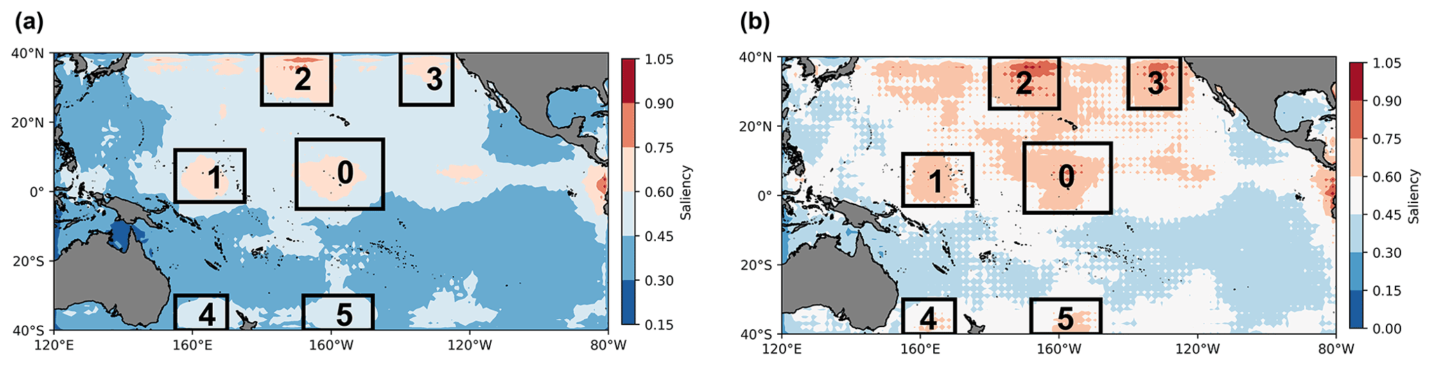
Figure 18The composite saliency maps of surface (a) and subsurface (b) layers over 40∘ N–40∘ S, 120∘ E–80∘ W. The higher the saliency value, the more sensitive the area. Since the saliency map results obtained from the surface layer and the subsurface layer may affect each other, we first select six common areas with large values as candidates to perform sensitivity experiments. The six areas are the central equatorial Pacific (0), the western equatorial Pacific (1), the northern central Pacific (2), the northeastern Pacific (3), the southwestern Pacific (4) and the southern central Pacific (5).
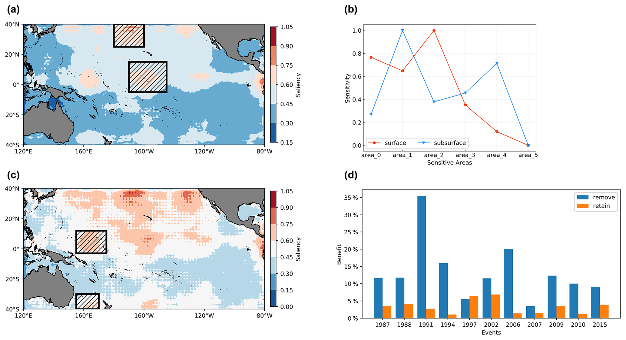
Figure 19Sensitive areas identification results for ENSO with the saliency map method. Panel (b) compares the sensitivity of the six candidate areas (0–5) for surface (red line) and subsurface (blue line). The first two most sensitive areas are selected as the sensitive areas of targeted observation for ENSO, that is, the area_0 and area_2 for surface and the area_1 and area_4 for subsurface layers, specifically, the hatched areas in (a) (surface) and (c) (subsurface). In order to evaluate the effectiveness of the above identified sensitive areas, (d) compares the benefit of removing the random perturbations in the sensitive areas (blue bars) and removing the random perturbations outside the sensitive areas (orange bars) (that is, retaining the random perturbations in the sensitive areas) for the eight El Niño events and three La Niña events which occurred in the past 30 years.
Furthermore, we perform two sets of experiments to measure the benefit of effective observations in the identified sensitive areas for improving forecast results. The first set calculates the reduction in the prediction error after removing the random perturbations in the identified sensitive areas (“remove”), and the second calculates the reduction after removing the perturbations outside the sensitive areas, that is, there are perturbations in the hatched areas in Fig. 19a, c (“retain”). For each ENSO event, we superimpose 30 groups of random perturbations on the original input field, select the random perturbations k whose errors are larger than the mean error of all groups and then conduct experiment “remove” and experiment “retain” respectively. Then we calculate the benefit Bremove and Bretain, where Vin is the volume of the identified sensitive areas and Vout is the volume outside the sensitive areas:
Bremove represents the degree of reduction in prediction errors after implementing target observation in per volume of identified sensitive areas shown in Fig. 19a and c, and Bretain represents the reduction after implementing target observation in per volume of non-sensitive areas (the outside areas of hatched regions in Fig. 19a, c). The results demonstrate that if the perturbations in the sensitive areas or those outside of the sensitive areas are eliminated, the prediction errors of ENSO can be reduced. However, due to the small size of the sensitive areas, the benefit obtained by removing random perturbations in the sensitive areas is relatively high (Fig. 19d), except for the super-strong El Niño event in 1997. Therefore, it is reasonable to give priority to effective observations in these identified sensitive areas, which are located in the central equatorial Pacific and the northern central Pacific surface region, and the western equatorial Pacific and the southwestern Pacific subsurface region. The results for the equatorial region support the conclusions of Kumar et al. (2014) and Duan and Hu (2016) in previous studies. Kumar et al. suggested that the observations in the central Pacific are more crucial than those in the eastern Pacific because of their role in preserving the memory of ENSO evolution. Duan and Hu emphasized the importance of subsurface signals in the western Pacific for ENSO predictions, which can influence the surface through equatorial waves and thermodynamic effects. However, due to the complexity of different models having a great impact on the identification of sensitive areas, there is no consistent conclusion about the sensitive areas of ENSO at present. For example, based on the outputs of the CMIP5 model, Zhang et al. (2015) identified the central-eastern equatorial surface region and eastern subsurface region as the sensitive areas. Therefore, determining the most appropriate regions for target observation remains a long-standing challenge. Nevertheless, such studies based on interpretability can improve our understanding of how the ENSO-MC model works in ENSO prediction. The results of sensitive area identification support the theoretical understanding that oceanic thermal anomaly in the central and western Pacific provides a key long-term memory for SST predictions. In addition, the results show that processes outside the tropical Pacific, such as surface temperature variations in the northern central Pacific and subsurface thermal changes in the southwestern Pacific, also have an impact on ENSO prediction.
With the successful application of deep learning algorithms in ENSO forecasts, this paper attempts to expand the application scope of deep neural networks from prediction to a broader field, including the pattern simulation, understanding and observation of ENSO. For reliable forecasts of the two types of ENSO, a multichannel data-driven model, ENSO-MC, is proposed to simulate the diversity of spatial patterns during ENSO events. Based on the ENSO-MC model, we then provide a new and promising approach to investigate the early signals of different types of ENSO events and identify the sensitive areas with the help of the saliency map interpretability method.
Specifically, the model ENSO-MC driven with oceanic and atmospheric predictors is proposed to simulate the ocean–atmosphere coupling process and predict the changes in spatial distribution of sea surface temperature anomalies. The simulation results show that the model can predict the development of SST anomalies in the equatorial Pacific during the onset, growth, maturity and decay of the El Niño and La Niña events 1 year in advance. In particular, we simulate the changes in the SST anomalies field of typical EP-type El Niños and CP-type El Niños at a lead time beyond 1 year. With the SST pattern forecasts, the all-season correlation skill of the Niño 3.4 index in the ENSO-MC model is also evaluated, which is above 0.5 for a lead of 11 months. The precursor maps reveal the different pronounced characteristics of the subsurface signals before the EP-type El Niño, CP-type El Niño and La Niña events. The results indicate that the EP-type El Niño is more related to the tropical thermocline dynamics, and the subtropical precursors seem to favour the generation of the CP-type El Niño. Both types of events have pronounced precursory signals in the northeastern Pacific whose distribution is similar to PMM. Before the La Niña events, there is an obvious subsurface signal propagating eastward from the equatorial western Pacific, which would shoal the thermocline in the eastern Pacific and trigger a cold event. In addition, we present an attempt of the saliency method based on the ENSO-MC model for sensitive area identification of ENSO. The identification results show that the surface sensitive areas are located in the central equatorial Pacific and the northern central Pacific, and the subsurface sensitive areas are concentrated in the western equatorial Pacific and the southwestern Pacific. Additional observations in these areas are expected to better predict an event in the future. It indicates that in equatorial regions, the central surface area and the western subsurface area will play an important role in the occurrence of future ENSO events, which are essential for preserving the memory of ENSO evolution. Furthermore, the processes in the extratropical Pacific, such as changes in the surface layer of the northern central Pacific and the subsurface layer of the southwestern Pacific, also contribute to ENSO prediction.
Since the cumulative error of the Niño 3.4 index calculated by predicting SST anomalies patterns is larger, the correlation skill is not as high as that obtained by predicting the index directly. Further research should be undertaken to explore how to ensure high correlation skills of the Niño 3.4 index while correctly simulating the spatial distribution of SST anomalies. In addition to the existing components of the ENSO-MC model, how to effectively use our existing domain knowledge, such as conservation of mass, conservation of salinity and other physical laws, to build a physics-informed ENSO-MC model that may help reduce uncertainty and increase the credibility of predictions is of great importance. For the precursor investigation, this paper focuses on verifying the known ENSO mechanisms, and the unknown inherent characteristics exploration will be considered in the future. Combining a structural causal model would help to extract the unknown causality relationships among factors and phenomena in ENSO complex interactions in this context. This would help further exploration of the precursors of ENSO and improve our understanding of its predictability.
The source code of the ENSO-MC 1.0 is available at https://doi.org/10.5281/zenodo.5725987 (Cui, 2021). Thanks to Computational and Information Systems Laboratory (CISL) of NCAR, IRI/LDEO Climate Data Library, NOAA/OAR/ESRL PSL and ECMWF for providing the historical reanalysis data (https://rda.ucar.edu/, Rayner et al., 2003); and (https://iridl.ldeo.columbia.edu/, Giese and Ray, 2011); (https://psl.noaa.gov/data/gridded/, Reynolds et al., 2002; Behringer and Xue, 2004); (https://apps.ecmwf.int/datasets/, Dee et al., 2011).
All authors designed the experiments and carried them out. YC developed the model code and performed the experiments. BM and BQ reviewed and optimized the code and experiments. YC and SY prepared the manuscript with contributions from all co-authors.
The contact author has declared that neither they nor their co-authors have any competing interests.
Publisher’s note: Copernicus Publications remains neutral with regard to jurisdictional claims in published maps and institutional affiliations.
This study was supported in part by the National Natural Science Foundation of China (grant no. U2142211), in part by the National Key Research and Development Program of China (grant no. 2020YFA0608002), in part by the National Natural Science Foundation of China (grant no. 42075141), in part by the Key Project Fund of Shanghai 2020 “Science and Technology Innovation Action Plan” for Social Development (grant no. 20dz1200702) and in part by the Fundamental Research Funds for the Central Universities (grant no. 13502150039/003).
This research has been supported by the National Natural Science Foundation of China (grant no. U2142211), the National Key Research and Development Program of China (grant no. 2020YFA0608002), the National Natural Science Foundation of China (grant no. 42075141), the Key Project Fund of Shanghai 2020 “Science and Technology Innovation Action Plan” for Social Development (grant no. 20dz1200702) and the Fundamental Research Funds for the Central Universities (grant no. 13502150039/003).
This paper was edited by Xiaomeng Huang and reviewed by two anonymous referees.
An, S.-I., Kug, J.-S., Timmermann, A., Kang, I.-S., and Timm, O.: The influence of ENSO on the generation of decadal variability in the North Pacific, J. Climate, 20, 667–680, 2007. a
Ashok, K., Behera, S. K., Rao, S. A., Weng, H., and Yamagata, T.: El Niño Modoki and its possible teleconnection, J. Geophys. Res.-Oceans, 112, C11007, https://doi.org/10.1029/2006JC003798, 2007. a
Behringer, D. and Xue, Y.: Evaluation of the global ocean data assimilation system at NCEP: The Pacific Ocean, in: Proc. Eighth Symp. on Integrated Observing and Assimilation Systems for Atmosphere, Oceans, and Land Surface, Seattle, WA., United States, 11–15 January 2004, https://origin.cpc.ncep.noaa.gov/products/people/yxue/pub/13.pdf (last access: 22 May 2022), 2004 (data available at: https://psl.noaa.gov/data/gridded/, last access: 10 February 2021). a
Bjerknes, J.: Atmospheric teleconnections from the equatorial Pacific, Mon. Weather Rev., 97, 163–172, 1969. a, b
Capotondi, A. and Sardeshmukh, P. D.: Optimal precursors of different types of ENSO events, Geophys. Res. Lett., 42, 9952–9960, 2015. a
Capotondi, A., Wittenberg, A. T., Newman, M., Di Lorenzo, E., Yu, J.-Y., Braconnot, P., Cole, J., Dewitte, B., Giese, B., Guilyardi, E., Jin, F.-F., Karnauskas, K., Kirtman, B., Lee, T., Schneider, N., Xue, Y., and Yeh, S.-W.: Understanding ENSO diversity, B. Am. Meteorol. Soc., 96, 921–938, 2015. a, b
Chen, D. and Cane, M. A.: El Niño prediction and predictability, J. Comput. Phys., 227, 3625–3640, 2008. a
Chen, D., Lian, T., Fu, C., Cane, M. A., Tang, Y., Murtugudde, R., Song, X., Wu, Q., and Zhou, L.: Strong influence of westerly wind bursts on El Niño diversity, Nat. Geosci., 8, 339–345, 2015. a
Chikamoto, Y., Timmermann, A., Luo, J.-J., Mochizuki, T., Kimoto, M., Watanabe, M., Ishii, M., Xie, S.-P., and Jin, F.-F.: Skilful multi-year predictions of tropical trans-basin climate variability, Nat. Commun., 6, 6869, https://doi.org/10.1038/ncomms7869, 2015. a
Cui, S.: Skye777/DL_ENSO-MC: First release of ENSO-MC deep learning model (v1.0.0), Zenodo [code], https://doi.org/10.5281/zenodo.5725987, 2021. a
Dee, D. P., Uppala, S. M., Simmons, A., Berrisford, P., Poli, P., Kobayashi, S., Andrae, U., Balmaseda, M., Balsamo, G., Bauer, D. P., Bechtold, P., Beljaars, A. C. M., van de Berg, L., Bidlot, J., Bormann, N., Delsol, C., Dragani, R., Fuentes, M., Geer, A. J., Haimberger, L., Healy, S. B., Hersbach, H., Holm, E. V., Isaksen, L., Kallberg, P., Koehler, M., Matricardi, M., McNally, A. P., Monge-Sanz, B. M., Morcrette, J.-J., Park, B.-K., Peubey, C., de Rosnay, P., Tavolato, C., Thepaut, J.-N., and Vitart, F.: The ERA-Interim reanalysis: Configuration and performance of the data assimilation system, Q. J. Roy. Meteor. Soc., 137, 553–597, https://doi.org/10.1002/qj.828, 2011 (data available at: https://apps.ecmwf.int/datasets/, last access: 15 February 2021). a
Duan, W. and Hu, J.: The initial errors that induce a significant “spring predictability barrier” for El Niño events and their implications for target observation: results from an earth system model, Clim. Dynam., 46, 3599–3615, 2016. a, b
Duan, W., Mu, M., and Wang, B.: Conditional nonlinear optimal perturbations as the optimal precursors for El Nino–Southern Oscillation events, J. Geophys. Res.-Atmos., 109, D23105 https://doi.org/10.1029/2004jd004756, 2004. a
Duan, W., Yu, Y., Xu, H., and Zhao, P.: Behaviors of nonlinearities modulating the El Niño events induced by optimal precursory disturbances, Clim. Dynam., 40, 1399–1413, 2013. a
Duan, W., Tian, B., and Xu, H.: Simulations of two types of El Niño events by an optimal forcing vector approach, Clim. Dynam., 43, 1677–1692, 2014. a
Duan, W., Huang, C., and Xu, H.: Nonlinearity modulating intensities and spatial structures of central Pacific and eastern Pacific El Niño events, Adv. Atmos. Sci., 34, 737–756, 2017. a
Ebert-Uphoff, I. and Hilburn, K.: Evaluation, tuning, and interpretation of neural networks for working with images in meteorological applications, B. Am. Meteorol. Soc., 101, E2149–E2170, 2020. a
Fedorov, A. V., Hu, S., Lengaigne, M., and Guilyardi, E.: The impact of westerly wind bursts and ocean initial state on the development, and diversity of El Niño events, Clim. Dynam., 44, 1381–1401, 2015. a
Gebbie, G., Eisenman, I., Wittenberg, A., and Tziperman, E.: Modulation of westerly wind bursts by sea surface temperature: A semistochastic feedback for ENSO, J. Atmos. Sci., 64, 3281–3295, 2007. a
Giese, B. S. and Ray, S.: El Niño variability in simple ocean data assimilation (SODA), 1871–2008, J. Geophys. Res.-Oceans, 116, C02024, https://doi.org/10.1029/2010JC006695, 2011 (data available at: https://iridl.ldeo.columbia.edu/, last access: 12 June 2021). a
Ham, Y.-G. and Kug, J.-S.: How well do current climate models simulate two types of El Niño?, Clim. Dynam., 39, 383–398, 2012. a
Ham, Y.-G., Kug, J.-S., Park, J.-Y., and Jin, F.-F.: Sea surface temperature in the north tropical Atlantic as a trigger for El Niño/Southern Oscillation events, Nat. Geosci., 6, 112–116, 2013. a
Ham, Y.-G., Kim, J.-H., and Luo, J.-J.: Deep learning for multi-year ENSO forecasts, Nature, 573, 568–572, 2019. a, b, c
Hu, J. and Duan, W.: Relationship between optimal precursory disturbances and optimally growing initial errors associated with ENSO events: Implications to target observations for ENSO prediction, J. Geophys. Res.-Oceans, 121, 2901–2917, 2016. a, b
Hu, S., Fedorov, A. V., Lengaigne, M., and Guilyardi, E.: The impact of westerly wind bursts on the diversity and predictability of El Niño events: An ocean energetics perspective, Geophys. Res. Lett., 41, 4654–4663, 2014. a
Huang, A., Vega-Westhoff, B., and Sriver, R. L.: Analyzing El Niño–Southern Oscillation Predictability Using Long-Short-Term-Memory Models, Earth and Space Science, 6, 212–221, 2019. a
Jin, F.-F.: An equatorial ocean recharge paradigm for ENSO. Part I: Conceptual model, J. Atmos. Sci., 54, 811–829, 1997a. a
Jin, F.-F.: An equatorial ocean recharge paradigm for ENSO. Part II: A stripped-down coupled model, J. Atmos. Sci., 54, 830–847, 1997b. a
Kao, H.-Y. and Yu, J.-Y.: Contrasting eastern-Pacific and central-Pacific types of ENSO, J. Climate, 22, 615–632, 2009. a
Kug, J.-S., Choi, J., An, S.-I., Jin, F.-F., and Wittenberg, A. T.: Warm pool and cold tongue El Niño events as simulated by the GFDL 2.1 coupled GCM, J. Climate, 23, 1226–1239, 2010. a
Kug, J.-S., Ham, Y.-G., Lee, J.-Y., and Jin, F.-F.: Improved simulation of two types of El Niño in CMIP5 models, Environ. Res. Lett., 7, 034002, https://doi.org/10.1088/1748-9326/7/3/034002, 2012. a
Kumar, A., Wang, H., Xue, Y., and Wang, W.: How much of monthly subsurface temperature variability in the equatorial Pacific can be recovered by the specification of sea surface temperatures?, J. Climate, 27, 1559–1577, 2014. a, b
Latif, M., Biercamp, J., and Von Storch, H.: The response of a coupled ocean-atmosphere general circulation model to wind bursts, J. Atmos. Sci., 45, 964–979, 1988. a
Lee, T. and McPhaden, M. J.: Increasing intensity of El Niño in the central-equatorial Pacific, Geophys. Res. Lett., 37, L14603, https://doi.org/10.1029/2010GL044007, 2010. a
Lingjiang, T. and Wansuo, D.: Using a nonlinear forcing singular vector approach to reduce model error effects in ENSO forecasting, Weather Forecast., 34, 1321–1342, 2019. a
Mathieu, M., Couprie, C., and LeCun, Y.: Deep multi-scale video prediction beyond mean square error, arXiv [preprint], arXiv:1511.05440, 17 November 2015. a
McPhaden, M. J.: Tropical Pacific Ocean heat content variations and ENSO persistence barriers, Geophys. Res. Lett., 30, 1480, https://doi.org/10.1029/2003GL016872, 2003. a
Meinen, C. S. and McPhaden, M. J.: Observations of warm water volume changes in the equatorial Pacific and their relationship to El Niño and La Niña, J. Climate, 13, 3551–3559, 2000. a
Menkes, C. E., Lengaigne, M., Vialard, J., Puy, M., Marchesiello, P., Cravatte, S., and Cambon, G.: About the role of westerly wind events in the possible development of an El Niño in 2014, Geophys. Res. Lett., 41, 6476–6483, 2014. a
Mo, R., Ye, C., and Whitfield, P. H.: Application potential of four nontraditional similarity metrics in hydrometeorology, J. Hydrometeorol., 15, 1862–1880, 2014. a
Moore, A. M. and Kleeman, R.: The dynamics of error growth and predictability in a coupled model of ENSO, Q. J. Roy. Meteor. Soc., 122, 1405–1446, 1996. a
Moore, A. M. and Kleeman, R.: Stochastic forcing of ENSO by the intraseasonal oscillation, J. Climate, 12, 1199–1220, 1999. a
Mu, B., Peng, C., Yuan, S., and Chen, L.: ENSO forecasting over multiple time horizons using ConvLSTM network and rolling mechanism, in: 2019 International Joint Conference on Neural Networks (IJCNN), Budapest, Hungary, 14–19 July 2019, IEEE, pp. 1–8, https://doi.org/10.1109/IJCNN.2019.8851967, 2019. a
Mu, B., Qin, B., and Yuan, S.: ENSO-ASC 1.0.0: ENSO deep learning forecast model with a multivariate air–sea coupler, Geosci. Model Dev., 14, 6977–6999, https://doi.org/10.5194/gmd-14-6977-2021, 2021. a
Mu, M., Duan, W. S., and Wang, B.: Conditional nonlinear optimal perturbation and its applications, Nonlin. Processes Geophys., 10, 493–501, https://doi.org/10.5194/npg-10-493-2003, 2003. a
Mu, M., Yu, Y., Xu, H., and Gong, T.: Similarities between optimal precursors for ENSO events and optimally growing initial errors in El Niño predictions, Theor. Appl. Climatol., 115, 461–469, 2014. a
Mu, M., Duan, W., Chen, D., and Yu, W.: Target observations for improving initialization of high-impact ocean-atmospheric environmental events forecasting, Natl. Sci. Rev., 2, 226–236, 2015. a
Newman, M., Shin, S.-I., and Alexander, M. A.: Natural variation in ENSO flavors, Geophys. Res. Lett., 38, L14705, https://doi.org/10.1029/2011GL047658, 2011. a
Oprea, S., Martinez-Gonzalez, P., Garcia-Garcia, A., Castro-Vargas, J. A., Orts-Escolano, S., Garcia-Rodriguez, J., and Argyros, A.: A review on deep learning techniques for video prediction, IEEE Transactions on Pattern Analysis and Machine Intelligence, 44, 2806–2826, https://doi.org/10.1109/TPAMI.2020.3045007, 2020. a
Philander, S. G. H.: El Nino southern oscillation phenomena, Nature, 302, 295–301, 1983. a
Rayner, N., Parker, D. E., Horton, E., Folland, C. K., Alexander, L. V., Rowell, D., Kent, E. C., and Kaplan, A.: Global analyses of sea surface temperature, sea ice, and night marine air temperature since the late nineteenth century, J. Geophys. Res.-Atmos., 108, 4407, https://doi.org/10.1029/2002JD002670, 2003 (data available at: https://rda.ucar.edu/, last access: 10 February 2021). a
Reichstein, M., Camps-Valls, G., Stevens, B., Jung, M., Denzler, J., Carvalhais, N., and Prabhat: Deep learning and process understanding for data-driven Earth system science, Nature, 566, 195–204, 2019. a, b
Reynolds, R. W., Rayner, N. A., Smith, T. M., Stokes, D. C., and Wang, W.: An improved in situ and satellite SST analysis for climate, J. Climate, 15, 1609–1625, https://doi.org/10.1175/1520-0442(2002)015<1609:AIISAS>2.0.CO;2, 2002 (data available at: https://psl.noaa.gov/data/gridded/, last access: 10 February 2021). a
Santoso, A., Mcphaden, M. J., and Cai, W.: The defining characteristics of ENSO extremes and the strong 2015/2016 El Niño, Rev. Geophys., 55, 1079–1129, 2017. a
Shi, X. and Yeung, D.-Y.: Machine learning for spatiotemporal sequence forecasting: A survey, arXiv [preprint], arXiv:1808.06865, 21 August 2018. a
Simonyan, K., Vedaldi, A., and Zisserman, A.: Deep inside convolutional networks: Visualising image classification models and saliency maps, arXiv [preprint], arXiv:1312.6034, 20 December 2013. a
Smilkov, D., Thorat, N., Kim, B., Viégas, F., and Wattenberg, M.: SmoothGrad: removing noise by adding noise, arXiv [preprint], arXiv:1706.03825, 12 June 2017. a
Sutskever, I., Vinyals, O., and Le, Q. V.: Sequence to sequence learning with neural networks, in: Advances in neural information processing systems, arXiv [preprint], arXiv:1409.3215, 14 December 2014. a
Ben Taieb, S. and Hyndman, R.: Recursive and direct multi-step forecasting: the best of both worlds, Tech. Rep., Monash University, Department of Econometrics and Business Statistics, 2012. a
Tang, Y., Zhang, R.-H., Liu, T., Duan, W., Yang, D., Zheng, F., Ren, H., Lian, T., Gao, C., Chen, D., and Mu, M.: Progress in ENSO prediction and predictability study, Natl. Sci. Rev., 5, 826–839, 2018. a
Tao, L., Duan, W., and Vannitsem, S.: Improving forecasts of El Niño diversity: a nonlinear forcing singular vector approach, Clim. Dynam., 55, 739–754, 2020. a
Tian, B. and Duan, W.: Comparison of the initial errors most likely to cause a spring predictability barrier for two types of El Niño events, Clim. Dynam., 47, 779–792, 2016. a
Timmermann, A., An, S.-I., Kug, J.-S., Jin, F.-F., Cai, W., Capotondi, A., Cobb, K. M., Lengaigne, M., McPhaden, M. J., Stuecker, M. F., Stein, K., Wittenberg, A. T. , Yun, K.-S., Bayr, T., Chen, H.-C., Chikamoto, Y., Dewitte, B., Dommenget, D., Grothe, P., Guilyardi, E., Ham, Y.-G., Hayashi, M., Ineson, S., Kang, D., Kim, S., Kim, W., Lee, J.-Y., Li, T., Luo, J.-J., McGregor, S., Planton, Y., Power, S., Rashid, H., Ren, H.-L., Santoso, A., Takahashi, K., Todd, A., Wang, G. M., Wang, G. J., Xie, R. H., Yang, W.-H., Yeh, S.-W., Yoon, J., Zeller, E., and Zhang, X. B.: El Niño–southern oscillation complexity, Nature, 559, 535–545, 2018. a, b
Trenberth, K. E. and Stepaniak, D. P.: Indices of el Niño evolution, J. Climate, 14, 1697–1701, 2001. a
Vimont, D. J., Battisti, D. S., and Hirst, A. C.: The seasonal footprinting mechanism in the CSIRO general circulation models, J. Climate, 16, 2653–2667, 2003. a
Vimont, D. J., Alexander, M. A., and Newman, M.: Optimal growth of central and east Pacific ENSO events, Geophys. Res. Lett., 41, 4027–4034, 2014. a
Wang, Z., Bovik, A. C., and Lu, L.: Why is image quality assessment so difficult?, in: 2002 IEEE International conference on acoustics, speech, and signal processing, Orlando, FL, USA, 13–17 May 2002, vol. 4, IEEE, pp. IV–3313, https://doi.org/10.1109/ICASSP.2002.5745362, 2002. a
Xingjian, S., Chen, Z., Wang, H., Yeung, D.-Y., Wong, W.-K., and Woo, W.-c.: Convolutional LSTM network: A machine learning approach for precipitation nowcasting, in: Advances in neural information processing systems, arXiv [preprint], arXiv:1506.04214, 19 September 2015. a
Yan, J., Mu, L., Wang, L., Ranjan, R., and Zomaya, A. Y.: Temporal convolutional networks for the advance prediction of ENSO, Scientific Reports, 10, 8055, https://doi.org/10.1038/s41598-020-65070-5, 2020. a
Yu, J.-Y. and Kao, H.-Y.: Decadal changes of ENSO persistence barrier in SST and ocean heat content indices: 1958–2001, J. Geophys. Res.-Atmos., 112, D13106, https://doi.org/10.1029/2006JD007654, 2007. a
Yu, J.-Y. and Kim, S. T.: Relationships between extratropical sea level pressure variations and the central Pacific and eastern Pacific types of ENSO, J. Climate, 24, 708–720, 2011. a
Yu, J.-Y., Zou, Y., Kim, S. T., and Lee, T.: The changing impact of El Niño on US winter temperatures, Geophys. Res. Lett., 39, L15702, https://doi.org/10.1029/2012GL052483, 2012. a
Zeiler, M. D. and Fergus, R.: Visualizing and understanding convolutional networks, in: European conference on computer vision, Springer, pp. 818–833, https://doi.org/10.1007/978-3-319-10590-1_53, 2014. a
Zhang, J., Duan, W., and Zhi, X.: Using CMIP5 model outputs to investigate the initial errors that cause the “spring predictability barrier” for El Niño events, Science China Earth Sciences, 58, 685–696, 2015. a
Zhang, R.-H. and Levitus, S.: Interannual variability of the coupled tropical Pacific ocean–atmosphere system associated with the El Niño–Southern Oscillation, J. Climate, 10, 1312–1330, 1997. a
Zinke, J., Browning, S., Hoell, A., and Goodwin, I.: The West Pacific Gradient tracks ENSO and zonal Pacific sea surface temperature gradient during the last Millennium, Scientific Reports, 11, 20395, https://doi.org/10.1038/s41598-021-99738-3, 2021. a
- Abstract
- Introduction
- ENSO-MC: simulation model for the two types of ENSO
- Model performance evaluation
- Analysis of ENSO forecast skill
- Precursor analysis of the two types of ENSO
- Targeted observation sensitive area identification of ENSO
- Conclusions
- Code and data availability
- Author contributions
- Competing interests
- Disclaimer
- Acknowledgements
- Financial support
- Review statement
- References