Training a supermodel with noisy and sparse observations: a case study with CPT and the synch rule on SPEEDO – v.1

As an alternative to using the standard multi-model ensemble (MME) approach to combine the output of different models to improve prediction skill, models can also be combined dynamically to form a so-called supermodel. The supermodel approach enables a quicker correction of the model errors. In this study we connect different versions of SPEEDO, a global atmosphere-ocean-land model of intermediate complexity, into a supermodel. We focus on a weighted supermodel, in which the supermodel state is a weighted superposition of different imperfect model states. The estimation, “the training”, of the optimal weights of this combination is a critical aspect in the construction of a supermodel. In our previous works two algorithms were developed: (i) cross pollination in time (CPT)-based technique and (ii) a synchronization-based learning rule (synch rule). Those algorithms have so far been applied under the assumption of complete and noise-free observations. Here we go beyond and consider the more realistic case of noisy data that do not cover the full system's state and are not taken at each model's computational time step. We revise the training methods to cope with this observational scenario, while still being able to estimate accurate weights. In the synch rule an additional term is introduced to maintain physical balances, while in CPT nudging terms are added to let the models stay closer to the observations during training. Furthermore, we propose a novel formulation of the CPT method allowing the weights to be negative. This makes it possible for CPT to deal with cases in which the individual model biases have the same sign, a situation that hampers constructing a skillfully weighted supermodel based on positive weights. With these developments, both CPT and the synch rule have been made suitable to train a supermodel consisting of state of the art weather and climate models.

1 Introduction

Climate models are continuously improving over time. This is made evident by the succession of the Coupled Model Intercomparison Project (CMIP), which is currently in its sixth stage (Eyring et al., 2016). The CMIP models are used by the Intergovernmental Panel on Climate Change (IPCC) for its assessment reports. The model complexity is increasing and more processes can be resolved due to increased spatial and temporal resolutions. Nevertheless, the real climate system is too complex (Ghil and Lucarini, 2020) for any numerical model so that models will inevitably remain imperfect (Palmer and Stevens, 2019).

Given a set of imperfect models, one can combine them so that their combination has a greater forecast skill than each individual model independently. A common approach is to use the multi-model ensemble (MME) (Hagedorn et al., 2005). In the MME the individual model ensembles are constructed based on different initial conditions but propagated forward in time using the same model. After integration the ensembles from different models are combined. The MME is most importantly a very powerful and useful approach to account for and to represent the uncertainty. Furthermore, it is possible to achieve better statistics such as the mean; this is because errors tend to cancel each other out (Hagedorn et al., 2005). Generally, the models are equally weighted in an MME mean as is the case for, e.g., the CMIP runs in the IPCC reports. Another possibility is to calculate a so-called superensemble (Krishnamurti et al., 2016), where the model weights are trained on the basis of historical observations, e.g., in Hagedorn et al. (2005) and Doblas-Reyes et al. (2005). This is inherently a statistical method that does not take possible changes in the model regimes into account. A caveat is obviously that weights that are optimal for model behavior in the past do not necessarily convert into optimal weights for the future. To cope with this, a “dynamical” on the fly approach to combine models is desirable, in which we act on the model equations.

Along this line, in the supermodel approach models are combined during the simulation by sharing their own tendencies or states with each other, and not just their outputs as with the MME. This amounts to creating a new virtual model, the supermodel, that can potentially have better physical behavior than the individual models. By combining the models dynamically into a supermodel, model errors can be reduced at an earlier stage, potentially mitigating error propagation and correcting the dynamics. This is particularly helpful since the climate system is not linear, which causes initial errors to spread over different variables and regions. The simulated climate statistics of the supermodel are therefore expected to be superior to that from the combination of biased models. The supermodel not only improves the statistics of simulated climate as in the MME, it can also give an improved model trajectory if the models are adequately synchronized. This could be essential in order to predict a specific sequence of weather or climate events. Given that the individual model trajectories in a MME are “free” to evolve according to each of the model dynamics, their averaging may result in an overall cancellation of the individual variabilities.

The supermodel approach was originally developed using low-dimensional dynamical systems (van den Berge et al., 2011; Mirchev et al., 2012) and subsequently applied to a global quasi-geostrophic atmospheric model (Schevenhoven and Selten, 2017; Wiegerinck and Selten, 2017) and to a coupled atmosphere-ocean-land model of intermediate complexity called SPEEDO (Selten et al., 2017; Schevenhoven et al., 2019). A partial supermodel implementation using state of the art coupled ocean-atmosphere models and using real-world observations was presented in Shen et al. (2016). A crucial step in supermodeling is the training of the weights based on data. The first supermodel training schemes were based on the minimization of a cost function (van den Berge et al., 2011; Shen et al., 2016), an approach with high computational cost, relying on a large number of long model runs. Schevenhoven and Selten (2017) developed a computationally efficient training scheme based on cross pollination in time (CPT), a concept originally introduced by Smith (2001). In CPT, the models in an MME exchange states during the simulation. As a consequence, the CPT trajectory tends to explore a larger area of the phase space than the individual models, thus enhancing the chance to pass in the vicinity of an observation. Another efficient training method, referred to as the synch rule, was introduced by Selten et al. (2017). The method, originally developed by Duane et al. (2007) for parameter estimation, is based on the synchronization theory of different systems.

The SPEEDO experiments in Selten et al. (2017) and Schevenhoven et al. (2019) were applied in a noise-free observation framework. The “historical observations”, used to train the supermodel, were available at every model time step. In this paper, we make a step forward towards applying CPT and the synch rule in state of the art models and real-world observations. Real-world observations are not perfect and are not continuously available in time. We adapt the training methods, again in the context of SPEEDO, in order to produce accurate weights, in the context of sparse observations affected by Gaussian distributed noise.

The paper is structured as follows. Section 2 briefly describes the SPEEDO model, and redefines the definition of the weighted supermodel in the context of sparse in time observations. Section 3 describes the training schemes CPT and the synch rule as used in Schevenhoven et al. (2019), and introduces adaptations to the methods to cope with sparse and noisy observations. In Schevenhoven et al. (2019), the synch rule was able to produce negative weights, and this seemed very beneficial in case models share biases that cannot compensate for each other. In this paper, we also explore the possibility of negative weights for CPT. Section 4 presents this possibility, together with the results of the adaptations to CPT and the synch rule in order to make the methods suitable for training on the basis of sparse and noisy observations. We conclude in Sect. 5 with a comparison of both training methods and an outlook to their application in state of the art models.

2 Weighted supermodel

This section recalls the general structure of a weighted supermodel as defined in Schevenhoven et al. (2019), and summarizes the supermodel structure used with the coupled atmosphere-ocean-land model SPEEDO (Severijns and Hazeleger, 2010); full details can be found in Schevenhoven et al. (2019). We then describe how the supermodel formulations are modified to handle time-sparse noisy data.

In Schevenhoven et al. (2019) the weighted supermodel was defined by combining the tendencies of the individual models. In the case of two imperfect models with parametric error, the weighted supermodel reads:

$$\begin{array}{}\text{(1a)}& {\displaystyle }& {\displaystyle }{\dot{\mathit{x}}}_{\mathrm{1}}=\mathit{f}\left({\mathit{x}}_{\mathrm{s}},{\mathit{p}}_{\mathrm{1}}\right),\text{(1b)}& {\displaystyle }& {\displaystyle }{\dot{\mathit{x}}}_{\mathrm{2}}=\mathit{f}\left({\mathit{x}}_{\mathrm{s}},{\mathit{p}}_{\mathrm{2}}\right),\text{(1c)}& {\displaystyle }& {\displaystyle }{\dot{\mathit{x}}}_{\mathrm{s}}={\mathbf{W}}_{\mathrm{1}}{\dot{\mathit{x}}}_{\mathrm{1}}+{\mathbf{W}}_{\mathrm{2}}{\dot{\mathit{x}}}_{\mathrm{2}},\end{array}$$

where x_s∈ℝⁿ represents the supermodel state vector, f the nonlinear evolution function depending on the state x and on a number of adjustable parameters ${\mathit{p}}_{\mathrm{1},\mathrm{2}}\in {\mathbb{R}}^m$, and the diagonal matrices ${\mathbf{W}}_{\mathrm{1},\mathrm{2}}=\mathrm{diag}\left({\mathit{w}}_{\mathrm{1},\mathrm{2}}\right)$ with ${\mathit{w}}_{\mathrm{1},\mathrm{2}}\in {\mathbb{R}}^n$ denote the weights. Training a weighted supermodel implies training the weights w. In Schevenhoven et al. (2019), we initialized all models from the same initial conditions, and the tendencies were combined at each model's computational time step, δt, that was assumed to be the same among the imperfect models. This choice implied a substantial computational cost. Constructing a supermodel for real model and observational scenarios requires relaxing this assumption.

This leads us to redefine a weighted supermodel by combining individual models at every arbitrary ΔT>δt, such that:

$$\begin{array}{}\text{(2a)}& {\displaystyle }& {\displaystyle }{\dot{\mathit{x}}}_{\mathrm{1}}={\mathit{\delta }}_{\mathrm{mod}(t,\mathrm{\Delta }T)}\mathit{f}\left({\mathit{x}}_{\mathrm{s}},{\mathit{p}}_{\mathrm{1}}\right)+\left(\mathrm{1}-{\mathit{\delta }}_{\mathrm{mod}(t,\mathrm{\Delta }T)}\right)\mathit{f}\left({\mathit{x}}_{\mathrm{1}},{\mathit{p}}_{\mathrm{1}}\right),\text{(2b)}& {\displaystyle }& {\displaystyle }{\dot{\mathit{x}}}_{\mathrm{2}}={\mathit{\delta }}_{\mathrm{mod}(t,\mathrm{\Delta }T)}\mathit{f}\left({\mathit{x}}_{\mathrm{s}},{\mathit{p}}_{\mathrm{2}}\right)+\left(\mathrm{1}-{\mathit{\delta }}_{\mathrm{mod}(t,\mathrm{\Delta }T)}\right)\mathit{f}\left({\mathit{x}}_{\mathrm{2}},{\mathit{p}}_{\mathrm{2}}\right),\text{(2c)}& {\displaystyle }& {\displaystyle }{\mathit{x}}_{\mathrm{s}}={\mathbf{W}}_{\mathrm{1}}{\mathit{x}}_{\mathrm{1}}+{\mathbf{W}}_{\mathrm{2}}{\mathit{x}}_{\mathrm{2}}\mathrm{if}{\mathit{\delta }}_{\mathrm{mod}(t,\mathrm{\Delta }T)}=\mathrm{1},\end{array}$$

where, the Kronecker δ function takes the value 1 when $\mathrm{mod}(t,\mathrm{\Delta }T)=\mathrm{0}$, and zero otherwise. In the latter case no supermodel state is defined. Note that, in contrast to the original formulation of the weighted supermodel given in Eq. (1a–c), here the individual model states are combined instead of their tendencies. In fact, combining the model tendencies every ΔT>δt can result in a much less synchronized supermodel state, thus possibly leading to a supermodel with poor forecasting skill: a supermodel trajectory from models that are not adequately synchronized will suffer from variance reduction and smoothing. Weighting the states ensures a synchronized supermodel state every ΔT. In our experiments so far, the models share the same state space, such that the models can continue with the exact supermodel state x_s, implying perfect synchronization imposed between the models every ΔT. In this study, we choose to let ΔT coincide with the observation frequency. The maximum time between two subsequent observations in this study is 24 h, this is frequent enough to maintain synchronization between the models.

2.1 SPEEDO model

The coupled model SPEEDO consists of an atmospheric component (SPEEDY), that exchanges information with a land (LBM) and an ocean-sea-ice component (CLIO). Detailed descriptions of SPEEDO can be found in Severijns and Hazeleger (2010) and Selten et al. (2017). SPEEDY describes the evolution of the horizontal wind components U (east-west) and V (north-south), temperature T and specific humidity q at eight vertical levels plus the surface pressure p_s. The horizontal grid resolution has a spacing of 3.75^∘ (48×96 grid cells). SPEEDY exchanges moisture and heat with the land model, LBM, which uses three soil layers and up to two snow layers to close the hydrological cycle over land. The horizontal discretization of the LBM is the same as for SPEEDY. Moreover, SPEEDY exchanges heat, water, and momentum with the ocean model, CLIO. CLIO describes the evolution of ocean currents, temperature and salinity on a computational grid with 3^∘ horizontal resolution and 20 unevenly spaced layers in the vertical resolution. A three-layer thermodynamic-dynamic sea-ice model describes the evolution of sea ice.

The SPEEDO equations can be formally and compactly written as

$$\begin{array}{}\text{(3a)}& {\displaystyle }& {\displaystyle }\dot{\mathit{a}}={\mathit{f}}^{\mathrm{a}}\left(\mathit{a};{\mathit{p}}^{\mathrm{a}}\right)+{\mathit{g}}^{\mathrm{a}}\left({\mathit{e}}^{\mathrm{h}},{\mathit{e}}^{\mathrm{w}},{\mathit{e}}^{\mathrm{m}}\right),\text{(3b)}& {\displaystyle }& {\displaystyle }\dot{\mathit{o}}={\mathit{f}}^{\mathrm{o}}\left(\mathit{o};{\mathit{p}}^{\mathrm{o}}\right)+{\mathit{g}}^{\mathrm{o}}\left({\mathcal{P}}^{\mathrm{o}}{\mathit{e}}^{\mathrm{h}},{\mathcal{P}}^{\mathrm{o}}{\mathit{e}}^{\mathrm{w}},{\mathcal{P}}^{\mathrm{o}}{\mathit{e}}^{\mathrm{m}},{\mathcal{P}}^{\mathrm{o}}\mathit{r}\right),\text{(3c)}& {\displaystyle }& {\displaystyle }\dot{\mathit{l}}={\mathit{f}}^{\mathrm{l}}\left(\mathit{l};{\mathit{p}}^{\mathrm{l}}\right)+{\mathit{g}}^{\mathrm{l}}\left({\mathcal{P}}^{\mathrm{l}}{\mathit{e}}^{\mathrm{h}},{\mathcal{P}}^{\mathrm{l}}{\mathit{e}}^{\mathrm{w}},\mathit{r}\right),\end{array}$$

where a stands for atmosphere, o for ocean and sea-ice and l for land; e^h represents the heat exchange between the atmosphere and surface, e^w the water exchange, e^m the momentum exchange and r the river outflow describing the streaming of water from land to ocean. The exchange vectors depend on the state of the atmosphere and the surface, but this dependency is not made explicit in Eq. (3a–c) to simplify the notation. The projection operators 𝒫 represent the conservative regridding operations between the computational grids of the different model components. The nonlinear functions f represent the cumulative contribution of the modeled physical processes to the change in the state vectors, and depend on the values of the parameter vectors p. The nonlinear functions g describe how the exchange of heat, water and momentum between atmosphere, ocean and land affects the change of the state vectors.

2.1.1 Weighted supermodel based on SPEEDO

A supermodel based on SPEEDO is formed by combining imperfect atmosphere components SPEEDY through a weighted superposition of the states of the imperfect models. All imperfect atmospheres are each coupled to the same ocean and land model. Figure 1 provides a schematic representation of the supermodel constructed.

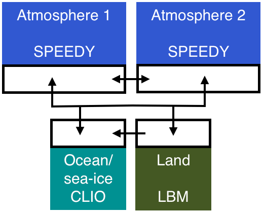
Figure 1 Schematic representation of the SPEEDO climate supermodel based on two imperfect atmospheric models. The two atmospheric models exchange water, heat and momentum with the perfect ocean and land model. The ocean and land model send their state information to both atmospheric models. The atmospheric models exchange state information in order to combine their states (Schevenhoven et al., 2019).

All the atmospheric components of the individual imperfect models receive the same state information from ocean and land. Nevertheless, each atmosphere calculates its own water, heat and momentum exchange. Conversely, the ocean and land components receive the multi-model weighted average of the atmospheric states. This supermodel construction is inspired by the interactive ensemble approach originally devised by Kirtman and Shukla (2002).

We can now write the SPEEDO weighted supermodel equations as

$$\begin{array}{}\text{(4a)}& {\displaystyle }\begin{array}{rl}{\dot{\mathit{a}}}_{\mathrm{i}}& =\left[{\mathit{\delta }}_{\mathrm{mod}(t,\mathrm{\Delta }T)}{\mathit{f}}^{\mathrm{a}}\left({\mathit{a}}_{\mathrm{s}};{\mathit{p}}_{\mathrm{i}}^{\mathrm{a}}\right)+\left(\mathrm{1}-{\mathit{\delta }}_{\mathrm{mod}(t,\mathrm{\Delta }T)}\right){\mathit{f}}^{\mathrm{a}}\left({\mathit{a}}_{\mathrm{i}};{\mathit{p}}_{\mathrm{i}}^{\mathrm{a}}\right)\right]\\ & +{\mathit{g}}^{\mathrm{a}}\left({\mathit{e}}_{\mathrm{i}}^{\mathrm{h}},{\mathit{e}}_{\mathrm{i}}^{\mathrm{w}},{\mathit{e}}_{\mathrm{i}}^{\mathrm{m}}\right),\end{array}\text{(4b)}& {\displaystyle }\begin{array}{rl}& \dot{\mathit{o}}={\mathit{f}}^{\mathrm{o}}\left(\mathit{o};{\mathit{p}}^{\mathrm{o}}\right)+{\mathit{g}}^{\mathrm{o}}\left({\mathcal{P}}^{\mathrm{o}}\stackrel{\mathrm{‾}}{{\mathit{e}}^{\mathrm{h}}},{\mathcal{P}}^{\mathrm{o}}\stackrel{\mathrm{‾}}{{\mathit{e}}^{\mathrm{w}}},{\mathcal{P}}^{\mathrm{o}}\stackrel{\mathrm{‾}}{{\mathit{e}}^{\mathrm{m}}},{\mathcal{P}}^{\mathrm{o}}\mathit{r}\right)\end{array},\end{array}$$

$$\begin{array}{}\text{(4c)}& {\displaystyle }\begin{array}{rl}& \dot{\mathit{l}}={\mathit{f}}^{\mathrm{l}}\left(\mathit{l};{\mathit{p}}^{\mathrm{l}}\right)+{\mathit{g}}^{\mathrm{l}}\left({\mathcal{P}}^{\mathrm{l}}\stackrel{\mathrm{‾}}{{\mathit{e}}^{\mathrm{h}}},{\mathcal{P}}^{\mathrm{l}}\stackrel{\mathrm{‾}}{{\mathit{e}}^{\mathrm{w}}},\mathit{r}\right),\end{array}\text{(4d)}& {\displaystyle }\begin{array}{rl}& {\mathit{a}}_{\mathrm{s}}=\sum _i{\mathbf{W}}_{\mathrm{i}}{\mathit{a}}_{\mathrm{i}}\mathrm{if}{\mathit{\delta }}_{\mathrm{mod}(t,\mathrm{\Delta }T)}=\mathrm{1},\end{array}\end{array}$$

where a_s denotes the atmospheric state of the supermodel, W_i the diagonal matrices with weights on the diagonal for the ith imperfect model, and the overbar indicates the weighted average over the models. At the instant times when a supermodel is constructed (i.e., δ=1), its state will be used to calculate the tendencies of the individual models. Otherwise, the individual models just continue their runs without interacting.

2.1.2 SPEEDO imperfect models

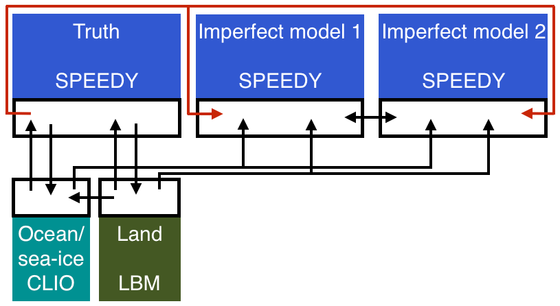
During the training for the supermodel based on SPEEDO, we regard the atmospheric model with standard parameter values as truth (Selten et al., 2017), whereas imperfect atmospheric models are created by perturbing those parameter values. The ocean and the land models receive the heat, water and momentum fluxes from the perfect atmospheric model only. All atmospheres receive the same information from the ocean and the land model, such that during training all imperfect atmospheres only deviate from the observations due to their own difference, not because of the coupling with ocean and land (see Fig. 2).

Figure 2 Schematic representation of the SPEEDO supermodel training (Selten et al., 2017).

We follow a similar experimental setup as in the precursor study by Schevenhoven et al. (2019); in particular, to simulate the imperfect models we perturb the same parameters with the same values. These are the convection relaxation timescale, the relative humidity threshold and the momentum diffusion timescale. The values used in the experiments are summarized in Table 1.

Table 1 Parameter values of perfect and imperfect models.

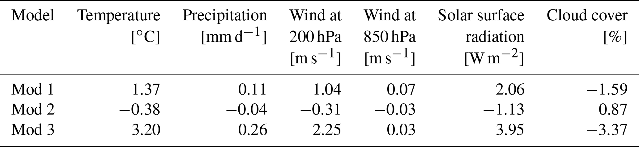
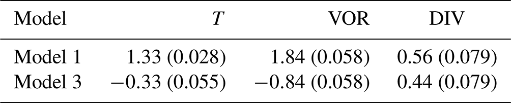
The impact of perturbing parameters on the models' climate (i.e., their long term behavior) is assessed on the basis of 40-year long simulations initiated on 1 January 2001. Table 2 shows the global mean average difference between the truth and the imperfect models for different variables. We see that the imperfect models 1 and 2 have biases with opposite signs in all of the variables. Note that their biases are comparable to those estimated for state of the art global climate models (Collins et al., 2013). The third model has biases in the same direction as model 1, but of generally larger amplitudes. We make use of models 1 and 3 for the experiments with negative weights.

Table 2 Global mean average difference between the imperfect models and the perfect model, calculated over the last 30 years of the simulation.

3 Training methods

3.1 Training with the synch rule

The synch rule was originally conceived for parameter optimization in Duane et al. (2007). We follow here a similar setting. Let us assume that the parameters q∈ℝ^m appear linearly in the system for state variables y∈ℝⁿ, such that $\dot{\mathit{y}}=\mathit{f}(\mathit{y};\mathit{q})$. The synch rule ensures convergence towards parameters p∈ℝ^m of the system for state variables x∈ℝⁿ, $\dot{\mathit{x}}=\mathit{f}(\mathit{x};\mathit{p})$, provided that synchronization between the systems occurs if the parameters of both systems are equal: y(t)→x(t) if p=q. The update of parameter q_j for the jth component of q reads:

$$\begin{array}{}\text{(5a)}& {\displaystyle }& {\displaystyle }\dot{\mathit{x}}=\mathit{f}(\mathit{x};\mathit{p}),\text{(5b)}& {\displaystyle }& {\displaystyle }\dot{\mathit{y}}=\mathit{f}(\mathit{y};\mathit{q})-\mathbf{K}(\mathit{y}-\mathit{x}),\end{array}$$

$$\begin{array}{}\text{(5c)}& {\dot{q}}_j=-{\mathit{\delta }}_j\sum _i{e}_i{\displaystyle \frac{\partial f_i(\mathit{y},\mathit{q})}{\partial q_j}},\end{array}$$

where f denotes the evolution function and K(y−x) a connecting term between the two systems that nudges y towards x. $\mathbf{K}\in {\mathbb{R}}^{n\times n}$ is a diagonal matrix of nudging coefficients, K=diag(k). Furthermore, $e_i=y_i-x_i$ denotes the ith component of the synchronization error, and δ_j an adjustable rate of the learning scaling factor.

We have extended the use of the synch rule to the training of supermodels (Selten et al., 2017; Schevenhoven et al., 2019). In this context q refers to the supermodel weights, y to the supermodel state and x to the observations. The synch rule is initialized with certain values for q and during training the weights are updated according to the rule, such that the supermodel synchronizes with the observations. In order to keep the supermodel in the vicinity of the observations, the supermodel is nudged towards the observations by the term K(y−x).

3.1.1 Nudging towards the observations

The sensitivity of the training results to the nudging strength K in SPEEDO was studied in Selten et al. (2017). It was found that an amount of $K=\mathrm{1}/\mathrm{24}$ h⁻¹ nudging was sufficient to let identical SPEEDO models synchronize with a small error of less than 0.2 ^∘C between the models. Nevertheless, in the experiments with different versions of SPEEDO, the synchronization error increases by one order of magnitude. This amount of nudging is suitable for training, since it keeps the models close enough to the observations. Furthermore, a clear distinction can be made between an untrained and a well-trained supermodel in terms of the synchronization error between the supermodel and the observations. Because in our experiments nudging is applied only when observations are available, we found that a stronger nudging term than in Selten et al. (2017) is needed (as is shown in Sect. 4), and that its amplitude is approximately inversely related to the number of observations. We have some flexibility in the choice of the nudging strength in view of a certain insensitivity of the results. For instance, there is a range of values of K for which identical SPEEDO models synchronize to each other while a large error is maintained between the different versions of SPEEDO. For the experiments in this paper K is therefore defined somehow arbitrarily, considering the fact that without nudging the error between models initially grows exponentially over time, but at some point saturates when the distance between the models is on average as the distance between two random states on their attractors. Additionally, K is chosen equal for all the connected variables.

3.2 Training with CPT

The CPT learning approach is based on an idea proposed by (Smith, 2001). It dynamically combines trajectories of different models, such that the solution space is virtually extended. The aim is to generate trajectories that more closely follow the truth. In (Schevenhoven and Selten, 2017), this idea has been developed into a supermodel training scheme.

The training phase of CPT starts from an observation. From the same initial state, the imperfect models run for a predefined cross pollination time, τ, until an observation is available. The individual model predictions are then compared to the observation, and the model state that is closest to the observation will serve as the initial condition for the next integration. In our experiments, the “closeness” to data is measured using the global root mean squared error (RMSE). In the case of a multidimensional (multivariate) model, such as SPEEDO, it is possible that at certain time steps different models are the closest to the truth for different state variables. In this case, the initial condition for the next run is constructed by combining the portion of the state vector of each closest model state. This choice, while providing the closest to data initial condition, is prone to create imbalances in the model integration. Nevertheless, we experienced that as long as the update is global, such that each grid point receives the state of the same model for a certain variable, these imbalances are not a big issue. Otherwise, a possible solution is to use techniques from data assimilation (Carrassi et al., 2018) to make the initial condition suitable for the individual models. An example is given in Du and Smith (2017) by using pseudo orbit data assimilation (PDA).

After the training, a CPT trajectory is obtained as a combination of different imperfect models, and we count how often each model has produced the best prediction of a particular component of the state vector during the training. These frequencies are then used to compute weights W for the corresponding states of the models. The superposition of the weighted imperfect model states forms the supermodel state. Since the frequency is used to compute the supermodel weights, the weights automatically sum to 1, which is also functional to maintain physical balances. See Schevenhoven and Selten (2017) for a more extensive and figurative explanation of the CPT training scheme.

3.2.1 The rationale behind CPT: an illustration

The CPT training method has been derived from a linear model assumption. Suppose we have two imperfect models with differential equations:

$$\begin{array}{}\text{(6a)}& {\displaystyle }& {\displaystyle }{\dot{x}}_{\mathrm{1}}={\mathit{\alpha }}_{\mathrm{1}},\text{(6b)}& {\displaystyle }& {\displaystyle }{\dot{x}}_{\mathrm{2}}={\mathit{\alpha }}_{\mathrm{2}},\end{array}$$

where $x_{\mathrm{1},\mathrm{2}}\in \mathbb{R}$ are state vectors and ${\mathit{\alpha }}_{\mathrm{1},\mathrm{2}}\in \mathbb{Q}$ scalar direction coefficients. Assume the perfect model equations are given by:

$$\begin{array}{}\text{(7)}& {\dot{x}}_T={\mathit{\alpha }}_T,\end{array}$$

where x_T∈ℝ and α_T∈ℚ. Furthermore, assume the imperfect models complement each other such that ${\mathit{\alpha }}_{\mathrm{1}}<{\mathit{\alpha }}_T<{\mathit{\alpha }}_{\mathrm{2}}$. Then there exists a convex combination ${\mathit{\alpha }}_{\mathrm{1}}\frac{n}{N}+{\mathit{\alpha }}_{\mathrm{2}}(\mathrm{1}-\frac{n}{N})={\mathit{\alpha }}_T$, with $n,N\in \mathbb{N}$ and n<N. Choosing model 1 n out of N time steps and N−n times model 2 will result in a CPT trajectory that after N time steps equals the perfect observation at that point in time. Constructing the CPT trajectory in such a way that the model closest to the observations is always chosen will result in an optimal trajectory.

Weather and climate models are chaotic instead of linear. The key to success is, however, not the dynamical nature of the models, i.e., whether they are linear or nonlinear, but the trade-off between the data sampling time and the regime of evolution of the differences among the individual model trajectories in between subsequent data times. If enough observations are available during training, the difference between the imperfect models between subsequent observation times can be described as quasi-linear, therefore still making it possible for the CPT training to work well. The obtained weights will not be perfect and possibly not as optimal as weights obtained with a cost function minimization approach. On the other hand, the results in Schevenhoven et al. (2019) show that in the short term the models are linear enough to let the CPT approach work well. Moreover, CPT is a very fast method, and only few iterations are necessary as compared to the common approach of minimization of a cost function.

3.2.2 Duration of the training time

In Schevenhoven et al. (2019), the CPT training period in SPEEDO was set to 1 week. The time step in these experiments was 15 minutes and observations were available at every time step. Therefore the weights were based on a trajectory consisting of 672 time steps, a number that leads to a quite accurate estimation of the weights. In this work on the other hand, we set the maximum time between two subsequent observations to 24 h, reducing the CPT trajectory to only 7 steps in 1 week. Increasing the length of the training period is difficult because the supermodel trajectory may lose track of the observations during training. To avoid this, the maximum duration for the training period is set to 2 weeks for ΔT=24 h. To obtain more precise weights we use the iterative method.

3.2.3 Iterative method

In Schevenhoven and Selten (2017) an iterative method was proposed to obtain converged weights. The first iteration step gives a first estimate of the weights of the supermodel. At the next iteration, the supermodel resulting from the previous iteration is added as an extra imperfect model, and can thus potentially be the closest model to the observations. To calculate the new weights of the supermodel after the iteration, we adopt a simple linear approach. To see this, consider the case of two imperfect models, and assume that after an iteration the weights are $w_{\mathrm{1}}^{\mathrm{o}}$ for imperfect model 1 and hence $w_{\mathrm{2}}^{\mathrm{o}}=\mathrm{1}-w_{\mathrm{1}}^{\mathrm{o}}$ for imperfect model 2. If the weights after the next iteration are $w_{\mathrm{1}}^{\mathrm{n}}$ for imperfect model 1, $w_{\mathrm{2}}^{\mathrm{n}}$ for imperfect model 2 and $\mathrm{1}-w_{\mathrm{1}}^{\mathrm{n}}-w_{\mathrm{2}}^{\mathrm{n}}$ for the supermodel, then the new supermodel weights will be $w_{\mathrm{1}}^{\mathrm{n}}+w_{\mathrm{1}}^{\mathrm{o}}(\mathrm{1}-w_{\mathrm{1}}^{\mathrm{n}}-w_{\mathrm{2}}^{\mathrm{n}})$ for imperfect model 1 and $w_{\mathrm{2}}^{\mathrm{n}}+w_{\mathrm{2}}^{\mathrm{o}}(\mathrm{1}-w_{\mathrm{1}}^{\mathrm{n}}-w_{\mathrm{2}}^{\mathrm{n}})$ for imperfect model 2. The supermodel with these weights will replace the previous supermodel in the next iteration step. Ideally, the added supermodel is closer to the truth than the initial imperfect models. This can help to follow the observations for a longer period of time.

3.2.4 Nudging

For long training periods and/or noisy data, an iterative method might not be enough to let the CPT trajectory adequately follow the observations during training. A simple solution is to use a form of nudging towards the observations, similar to what is done in the synch rule. The equations for the CPT trajectory x_CPT with nudging, in an example with two imperfect models, are as follows:

$$\begin{array}{}\text{(8a)}& {\displaystyle }\begin{array}{rl}{\dot{\mathit{x}}}_{\mathrm{1}}& ={\mathit{\delta }}_{\mathrm{mod}(t,\mathrm{\Delta }T)}\left[\mathit{f}\left({\mathit{x}}_{\mathrm{CPT}},{\mathit{p}}_{\mathrm{1}}\right)+K\left({\mathit{x}}_{\mathrm{obs}}-{\mathit{x}}_{\mathrm{CPT}}\right)\right]\\ & +\left(\mathrm{1}-{\mathit{\delta }}_{\mathrm{mod}(t,\mathrm{\Delta }T)}\right)\mathit{f}\left({\mathit{x}}_{\mathrm{1}},{\mathit{p}}_{\mathrm{1}}\right)\end{array},\text{(8b)}& {\displaystyle }\begin{array}{rl}{\dot{\mathit{x}}}_{\mathrm{2}}& ={\mathit{\delta }}_{\mathrm{mod}(t,\mathrm{\Delta }T)}\left[\mathit{f}\left({\mathit{x}}_{\mathrm{CPT}},{\mathit{p}}_{\mathrm{2}}\right)+K\left({\mathit{x}}_{\mathrm{obs}}-{\mathit{x}}_{\mathrm{CPT}}\right)\right]\\ & +\left(\mathrm{1}-{\mathit{\delta }}_{\mathrm{mod}(t,\mathrm{\Delta }T)}\right)\mathit{f}\left({\mathit{x}}_{\mathrm{2}},{\mathit{p}}_{\mathrm{2}}\right)\end{array},\text{(8c)}& {\displaystyle }\begin{array}{rl}& {\mathit{x}}_{\mathrm{CPT}}=\\ & \left\{\begin{array}{ccl}{\mathit{x}}_{\mathrm{1}},& \mathrm{if}\Vert {\mathit{x}}_{\mathrm{1}}-{\mathit{x}}_{\mathrm{obs}}\Vert \le \Vert {\mathit{x}}_{\mathrm{2}}-{\mathit{x}}_{\mathrm{obs}}\Vert & \mathrm{and}{\mathit{\delta }}_{\mathrm{mod}(t,\mathrm{\Delta }T)}=\mathrm{1}\\ {\mathit{x}}_{\mathrm{2}},& \mathrm{if}\Vert {\mathit{x}}_{\mathrm{2}}-{\mathit{x}}_{\mathrm{obs}}\Vert \le \Vert {\mathit{x}}_{\mathrm{1}}-{\mathit{x}}_{\mathrm{obs}}\Vert & \mathrm{and}{\mathit{\delta }}_{\mathrm{mod}(t,\mathrm{\Delta }T)}=\mathrm{1}\end{array}\right.\end{array},\end{array}$$

where x_obs  denote the observations, δ the Kronecker delta, ΔT the observation frequency and K the nudging coefficient. In the experiments in this section K is equal for all state variables. As with the synch rule, the nudging strength needs to be enough to follow the observations, but it should not be too strong. The goal of CPT is to see how models can compensate for each other. Therefore, deviations from the original observations can be advantageous as long as there are imperfect models able to counteract this deviation. Nudging the imperfect model states to a value very close to the observations will lead to a too frequent choice of the model that is on average closest to the observations, thus limiting the diversity of representation within the supermodel.

4 Results

4.1 Training in SPEEDO

Before we start training the supermodel, we need to decide when, where and how to let the models exchange their information in order to create a weighted supermodel.

Following Schevenhoven et al. (2019), we use global weights for both CPT and the synch rule. This means that we use the same weight for all grid points. By doing so we mitigate, and in the best case prevent, numerical instabilities; however, note that different weights are allowed for each variable.

As long as there are enough observations to capture the global behavior of the different models, spatially sparse observations are not expected to be an issue when constructing a weighted supermodel. Given that we focus here on the data sparsity in time, in the experiments we assume that all grid points are observed.

The prognostic variables exchanged between models are temperature, vorticity and flow divergence. The weights for the fluxes from atmosphere to ocean and to land are given by the average of the weights for the three prognostic variables. The SPEEDO time step during training is set to δt=15 min.

Following Schevenhoven et al. (2019), the training period for both CPT and the synch rule is 1 year. For CPT, the supermodel weights are calculated every week or every second week in the case of ΔT=24 h, and the model states are set back to the observations. For the synch rule the training period continues for an entire year. This amount of time is needed to obtain stable converged weights.

The codes for both training methods of CPT and the synch rule in the experiments in this paper are integrated into the SPEEDO code. After the individual models have made their individual time steps, their states are exchanged between the models with coupling routines. Once all models have shared their knowledge, they can calculate the new supermodel state and the update of the weight according to the training method. The SPEEDO CPT and synch rule supermodel training code is available in Schevenhoven (2021).

4.2 Synch rule adaptations

In Schevenhoven et al. (2019) the synch rule, rewritten from Eq. (5a–c), looked as follows:

$$\begin{array}{}\text{(9)}& {\dot{W}}_{i,j}=-{\mathit{\delta }}_j{e}_j{f}_{i,j},\end{array}$$

where W_i,j denotes the weight of model i for state variable j, f_i,j the imperfect model tendency of model i and state variable j, e_j the synchronization error between the supermodel state and the observations, and δ_j an adjustable rate of the learning scaling factor. This equation is derived without any prior assumption on the weights. In the context of noise-free and continuously available observations, the weights turned out to sum approximately to 1, which seems necessary in order to maintain physical balances. Nevertheless, when Eq. (9) is used in the case of noisy and sparse in time observations, the weights do not sum to 1 anymore. If the deviation from 1 is too large, the supermodel state will be either too small or too large compared to the imperfect model states, possibly resulting in loss of synchronization with the observations and an even worse estimation of the next weight update.

We adapt the synch rule such that the weights are imposed to sum to 1. This is achieved by using the tendency of the individual imperfect model f_i, but also by subtracting the equally weighted supermodel tendency $f_{\mathrm{E}}=\frac{\mathrm{1}}{N}\sum _{i=\mathrm{1}}^N{f}_i$. The new synch rule is defined as (see Appendix A for a derivation):

$$\begin{array}{}\text{(10)}& {\dot{W}}_i=-\mathit{\delta }e\left(f_i-f_{\mathrm{E}}\right),\end{array}$$

where index j is omitted to simplify the notation. From Eq. (10) it can be seen that the total update of the weights for the N imperfect models equals 0: $\sum _{i=\mathrm{1}}^N{\dot{W}}_i=-\mathit{\delta }e\sum _{i=\mathrm{1}}^N(f_i-f_{\mathrm{E}})=-\mathit{\delta }eN(f_{\mathrm{E}}-f_{\mathrm{E}})=\mathrm{0}$. Thus, if the initial weights sum to 1, they will sum to 1 continuously throughout the training.

4.2.1 Adaptation to nudging

Too little nudging towards the observations during training may lead to large errors between the imperfect models and the observations. In this case, the updates of the weights might go in a different direction than anticipated. The imperfect models and the observations might be in different phases, resulting in a converse sign of the synchronization error e. Interestingly, it is still possible to obtain converged weights in this case, only that the weights differ substantially from those obtained with more nudging towards the observations.

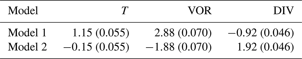
In the first experiment of (Schevenhoven et al., 2019) the weights for temperature (T), vorticity (VOR) and divergence (DIV) all turned out to be around 0.3 for imperfect model 1 and 0.7 for imperfect model 2. We apply the same amount of nudging to the same imperfect models, except that the observations are available every second time step, instead of every time step. Then the weights converge to the weights given in Table 3.

Table 3 Weights for the supermodel trained by the synch rule with an observation available at every second time step and the same amount of nudging towards the observations as in Selten et al. (2017) and Schevenhoven et al. (2019). The weights are averaged over the last 10 weeks of training. The standard deviation is given in parentheses.

When the weights converge towards stable values as in Table 3, the average update of the weights must be equal to 0. Hence, at least one of the terms in Eq. (10) should be equal to 0 on average. Since the imperfect models are not yet in equilibrium after 1 year (Schevenhoven et al., 2019), the average model tendency cannot be 0. This implies that the error between the supermodel and the observations must be equal to 0; however, a free run of 40 years with a supermodel with the weights from Table 3 results in a climatological error of up to +2 ^∘C in the Northern Hemisphere and up to −2 ^∘C in the Southern Hemisphere. Thus, too little nudging during training can result in a supermodel with a correct global average temperature (the opposite biases on the two hemispheres cancel out), but very different dynamics compared to the observations.

There can also be too much nudging towards observations. In this case, a link with data assimilation can be made, where one has to find a middle ground between noisy observations and the model. Too much nudging towards the observations during training can result again in a converse sign of the synchronization error e. This leads to an incorrect update of the weights, making it more difficult to follow the observations during training.

4.3 Limitations of sparse and noisy observations

In this section we assess to what extent observations can be noisy and sparse in time before the CPT or the synch rule training methods are no longer able to produce weights close to the optimum. To systematically evaluate this, we choose 4 different observation frequencies ΔT: 15 min, 1 h, 6 h and 24 h. Since for the standard CPT training time of 1 week the weights for ΔT=24 h would only be based on 7 steps, the training time for this observation frequency is doubled to 2 weeks. The error in the observations is unbiased and Gaussian distributed $\sim N(\mathrm{0},\mathit{\sigma })$, where standard deviation σ is chosen to be equal to either 0.5 %, 2.5 % or 5 % of the spatial standard deviation σ_X of the observations per prognostic variable X. Hence ${\mathit{\sigma }}_X=\frac{\mathrm{1}}{N}\sqrt{\sum _i{\left(X_i-\stackrel{\mathrm{‾}}{X}\right)}^{\mathrm{2}}}$, with i ranging over all $N=\mathrm{96}\times \mathrm{48}\times \mathrm{8}$ grid points and $\stackrel{\mathrm{‾}}{X}$ denoting the spatial mean value. For temperature this corresponds to a standard deviation of ∼0.15, 0.75 and 1.5 ^∘C. Table 4 denotes the chosen nudging coefficient K and the resulting weights together with their variance. For the experiments with Δt=15 min the same nudging strength K is chosen as in Schevenhoven et al. (2019): $K=\mathrm{1}/\mathrm{24}$ h⁻¹, which corresponds to K=1 d⁻¹. All CPT experiments are performed with the iterative method.

Table 4 Weights for the supermodel trained by CPT and the synch rule. The standard deviation over the year (CPT) or the standard deviation over the last 10 weeks of training (synch rule) is given in parentheses. The weights are only given for model 1, for model 2 the weight equals 1 − weight of model 1.

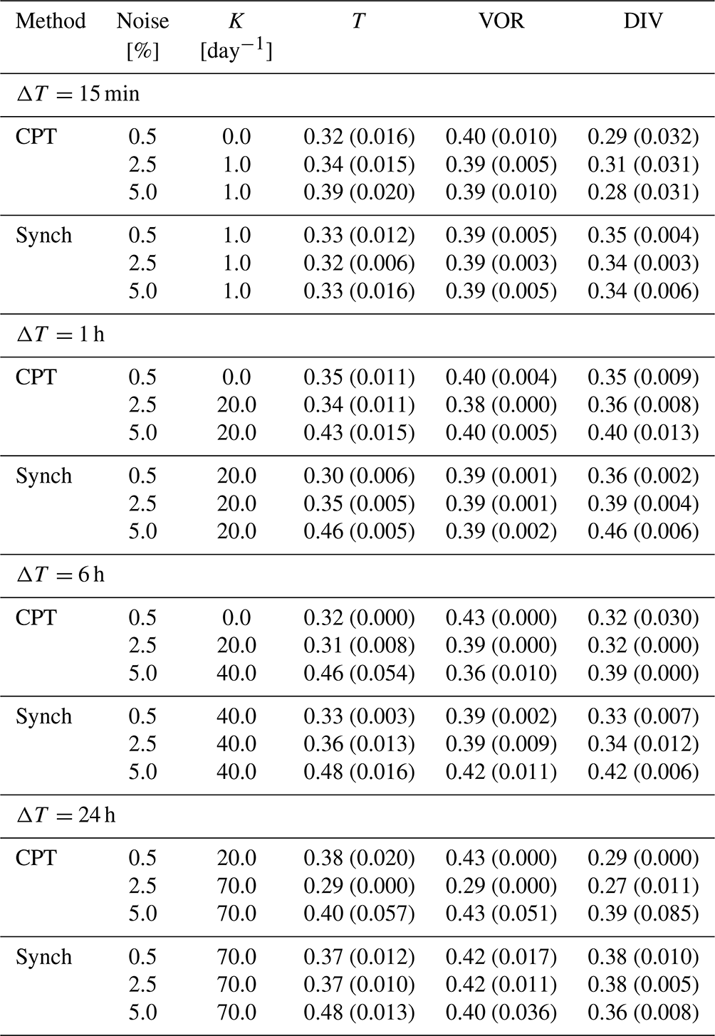
Figure 3 shows the weights from Table 4 in one plot such that the differences between the methods become clear. The horizontal lines (continuous for model 1 and dashed for model 2) indicate the weights obtained by CPT and the synch rule in Schevenhoven et al. (2019), in which case the observations were perfect and available at every time step. Despite the optimal weights for ΔT=15 min they are not necessarily expected to be optimal for, e.g., ΔT=24 h, in this particular experiment the 2 cases show similar weights. From Fig. 3a and b it can be seen that if observations are available at each time step (ΔT=15 min), the synch rule gives slightly better results for noisier observations than CPT. For the synch rule, the weights turn out to be almost exactly the same for all three levels of noise. For ΔT=1 h, the results for CPT and the synch rule seem similar for the two lowest noise levels. For the highest noise level, both methods seem to struggle a bit more to obtain good weights, since the models are more equally weighted. Decreasing the observation frequency further to ΔT=6 h results in the same pattern with CPT performing slightly better. Once good CPT weights have been found, they remain very consistent throughout the year, indicated by the standard deviation of 0. For the largest observation window ΔT=24 h, again the synch rule seems to encounter somewhat more difficulties in following the temperature observations for the highest noise level. Overall however, both methods perform well in the context of sparse and noisy observations.

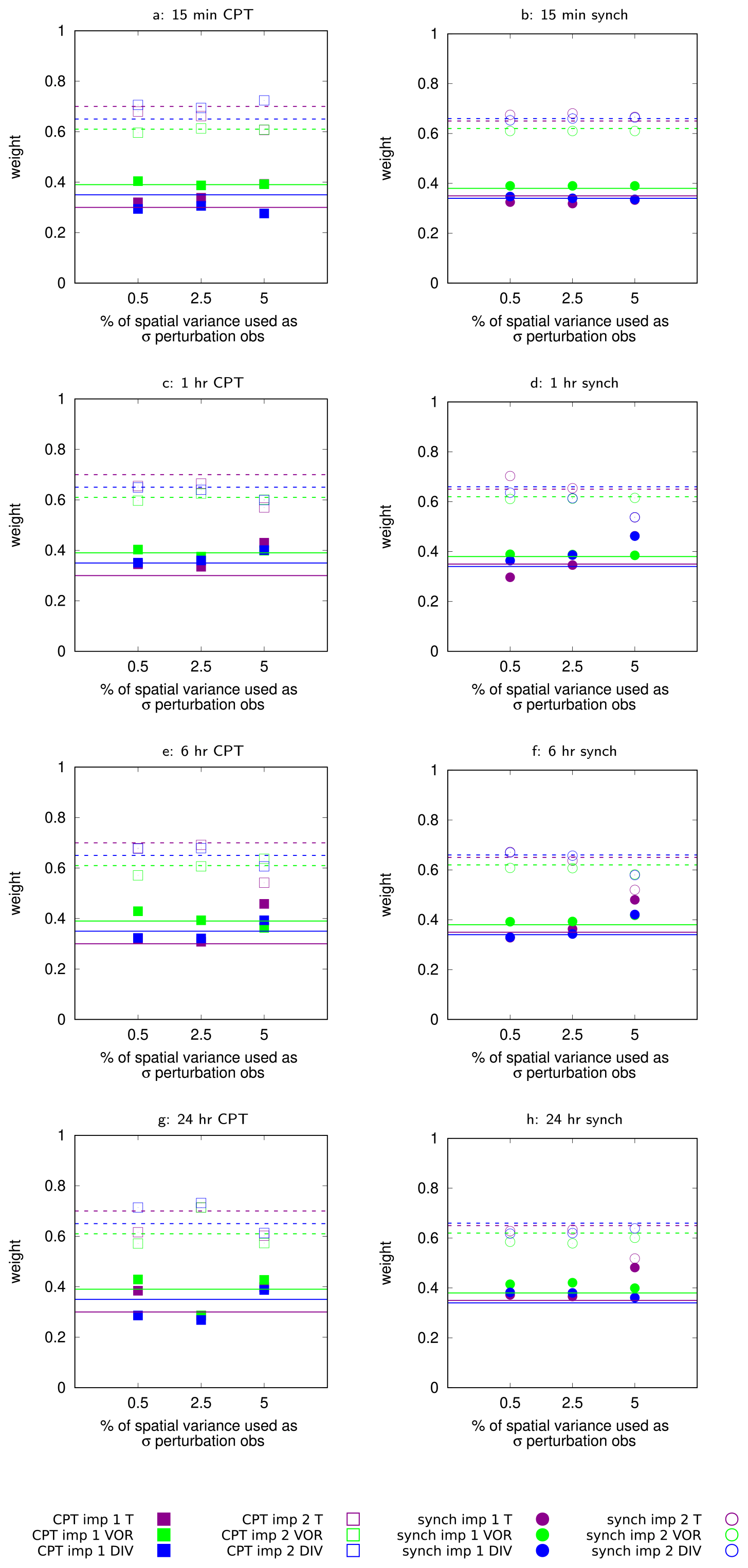
Figure 3 Weights for the supermodel trained by CPT and the synch rule. The horizontal lines (continuous for model 1, dashed for model 2) indicate the weights obtained by CPT and synch rule training in Schevenhoven et al. (2019), in which case the observations were perfect and available at every time step.

From Schevenhoven et al. (2019) we know the performance of supermodels with CPT and synch rule weights trained with perfect, noise free observations. The weights for the different experiments in Schevenhoven et al. (2019) varied within a range of ±0.05 per variable. We did not find any significant difference in the forecast performance of the supermodels for these weights. Since the weights in the experiments in this paper are approximately within this range, we can foresee the outcome of model performance experiments. To see this point, we compared the short-term forecast performance of the supermodels trained by perfect observations (s-CPT/synch perf obs), and the supermodels trained by observations available every 24 h(s-CPT/synch noisy obs), with the highest noise level we used in this paper (see Fig. 4). Not surprisingly, the supermodels trained with perfect observations are slightly better than the two supermodels trained with sparse and noisy observations. The supermodels trained with the observations available every 24 h, also combine in the forecast phase the states every 24 h, which introduces a small shock. The supermodel differences in the 2-week forecast, however, are very small. The synch rule supermodel trained with sparse and noisy observations performs least well, but one would expect this result as the weights for temperature are clearly a bit different from the other supermodels. Still, the model skill is not far from the other supermodel skills.

Figure 4 Forecast quality as measured by the RMSE of the truth and a model with a perturbed initial condition. The control is the difference between the perfect model and the perfect model with a perturbed initial condition. The pink and orange lines show the supermodels trained by perfect observations (s-CPT/synch perf obs), and the supermodels trained by observations available every 24 h (s-CPT/synch noisy obs),respectively, with the highest noise level used in this paper.

4.4 Negative weights

Imperfect models 1 and 2 complement each other in important physical variables such as temperature and wind. Model 1 tends to overestimate their global average values, while model 2 underestimates them. Together they form a convex hull (Schevenhoven and Selten, 2017), which results in positive supermodel weights. On the other hand, using model 1 and model 3 to construct a supermodel implies the need for negative weights. The synch rule naturally allows negative weights, since we did not impose any restrictions on the weights. In Schevenhoven et al. (2019) synch rule training has been performed with model 1 and model 3, resulting in a supermodel with partly negative weights that outperformed both imperfect models in short-term and long-term forecast quality.

CPT training does not automatically produce negative weights, since the weights are based on the frequency by which the imperfect models are chosen. Nevertheless, CPT training can give negative weights too, although with boundary restrictions. In the standard CPT training, one chooses whether one of the imperfect models is the closest to the observations, or in addition, whether the supermodel is closest in the iterative method. To obtain negative weights one can also choose a predefined combination of the imperfect models, for example: ${\mathit{x}}_{\mathrm{neg}\mathrm{1}}=\mathit{\alpha }{\mathit{x}}_{\mathrm{1}}+(\mathrm{1}-\mathit{\alpha }){\mathit{x}}_{\mathrm{3}}$, with α∈ℝ. If one defines an additional predefined combination ${\mathit{x}}_{\mathrm{neg}\mathrm{2}}=(\mathrm{1}-\mathit{\alpha }){\mathit{x}}_{\mathrm{1}}+\mathit{\alpha }{\mathit{x}}_{\mathrm{3}}$, the range for weights w₁ and w₃ for imperfect models 1 and 3 is between α and 1−α if $\mathit{\alpha }\notin [\mathrm{0},\mathrm{1}]$.

In this experiment we choose $\mathit{\alpha }=-\mathrm{1}$, such that w₁, ${\mathit{w}}_{\mathrm{3}}\in [-\mathrm{1},\mathrm{2}]$. The experiment is the same as in Schevenhoven et al. (2019): an observation is available for every time step , for every time step either x_neg1 or x_neg2 per variable is chosen as the closest model state and the training period is 1 week. Table 5 shows the weights and associated variance of the weights. The weights are remarkably similar to the weights of the synch rule experiment with negative weights in Schevenhoven et al. (2019). The weights for vorticity and divergence differ by 0.16, the weights for temperature by only 0.03.

Table 5 Weights for the supermodel trained by CPT allowing for negative weights. The standard deviation over the year is given in parentheses.

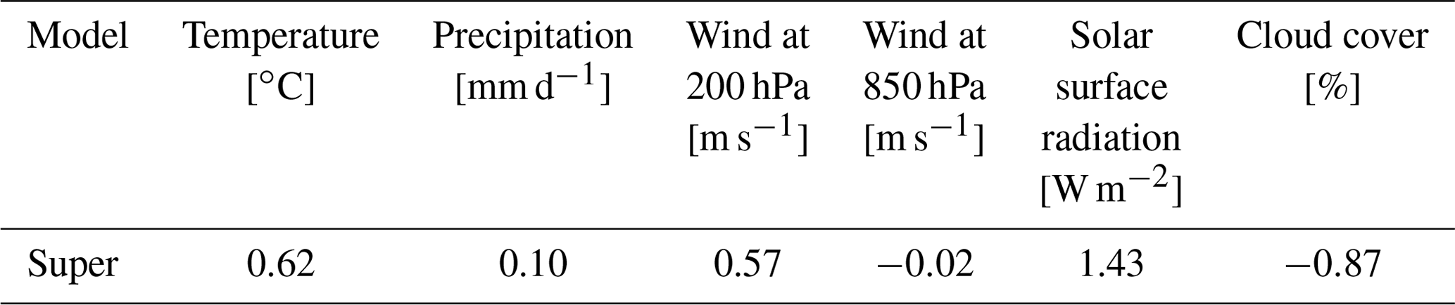
The statistics of a 40-year supermodel run with the weights from Table 5 are therefore quite similar to the climatology of the supermodel in Schevenhoven et al. (2019). Table 6 shows that the supermodel outperforms both imperfect models in temperature, precipitation, wind, cloud cover and surface solar radiation compared to the values in Table 2.

Table 6 Global mean average difference between the supermodel with negative weights and the perfect model, calculated over the last 30 years of the simulation.

5 Discussion and conclusion

We have shown the potential of the CPT and synch rule training methods to train a weighted supermodel on the basis of noisy and sparse time observations. The CPT training method is based on “crossing” different model trajectories and thus generating a larger ensemble of possible trajectories. The synch rule adapts the weights to the individual models on the fly during the training, such that the supermodel synchronizes with the observations. In our previous work (Schevenhoven et al., 2019) it was shown that both methods were able to improve weather and climate predictions in a noise-free and highly frequent observational setting, using different parametric versions of the global coupled atmosphere-ocean-land model SPEEDO. In this study, we moved towards realism by handling the case of noisy data that are not available at each of the models' computational time step. We have generated synthetic noisy observations by adding zero-mean Gaussian noise, with variance as large as 1.5 ^∘C in temperature. These synthetic noisy observations are made available at different intervals, of 1, 6 or 24 h. Both methods needed adaptations over the original formulations given in Schevenhoven et al. (2019) in order to train the weighted supermodel on the basis of noisy and sparse time observations. The new variants of the training methods have proven robustness against these changes in the observational scenario and shown capabilities to give adequate weights.

To handle noisy and sparse time data, we use nudging in both methods: this choice proved to be pivotal to ensure correct updates of the weights. For the synch rule the nudging strength was increased while for CPT the nudging term was not present in the original formulation and has been introduced here.

For the synch rule it is necessary that the sum of the weights remains equal to 1 in order to maintain physical balances. In the noise-free framework of Schevenhoven et al. (2019), this is ensured automatically. Nevertheless, in the current framework we had to impose the condition that the weights sum to 1, which is achieved by subtracting the equally weighted tendency term in the synch rule equation. Besides the inclusion of nudging in the CPT method, the use of an iterative approach within CPT further helped to keep track of the data. Additionally, in Schevenhoven et al. (2019) the synch rule was able to produce negative weights in case the imperfect models cannot compensate for each other's biases with positive weights. In this paper, we have gone beyond this and developed a method to obtain negative weights also within the CPT method.

The CPT and the synch rule both update the weights based on the difference between the model trajectories and the observations, and on the difference between the imperfect model tendencies. Despite using similar ingredients, CPT and the synch rule give different results for sparse and noisy observations. In particular, the synch rule trajectory seems to diverge slightly earlier from the observations than the CPT. A possible reason could be the different use of the models' tendencies. With CPT, the imperfect models run unconstrained from the data in the period, ΔT, between subsequent observations. If ΔT is large enough the model trajectories will have a large spread before being compared at the next observation time. Choosing the right model from this large spread can quickly reduce the distance to the observations. For the synch rule, on the other hand, one integrates the supermodel instead of the individual models as in CPT. Once the synch rule supermodel trajectory has diverged from the observations, it can be more difficult to get back to the observations compared to the CPT training, since the supermodel weights need to be adapted such that the next integration period will bring the supermodel closer to the observations. If ΔT is small, CPT and the synch rule are very comparable methods, as we have also seen in the results of the negative weight experiment in Sect. 4.

Future directions

Despite the application of the iterative method and nudging, the CPT and synch rule may still struggle to stay very close to the observations. To increase the chance to obtain a proper trajectory, one could work with an augmented ensemble of trajectories. This ensemble could consist of trajectories starting from slightly different initial conditions, or trajectories that emerge from a model nearby the closest model to an observation. One could make a comparison with the particle filter method (see e.g., van Leeuwen et al., 2019), where trajectories that do not fall within the likelihood of the observations are pruned and one continues with the trajectories within the likelihood of the observations from slightly perturbed initial conditions. In our case, the best trajectory after training can be obtained by comparing the RMSE between the trajectories and the observations.

Both training methods seem in principle more suitable for short rather than longer timescales, since for both training rules it is important that the imperfect models stay close enough to the observations. For longer timescales this can be difficult. Despite the action of the nudging, the models can be out of the data phase as long as time evolves. If the observations are lost, the “closest” model in the CPT training is not necessarily the one that contributes most to improving the supermodel dynamics. If during synch rule training the supermodel loses the observations, a new, non-optimal equilibrium for the weights can be found, as we have seen in Sect. 4. Having said this, both methods could still be useful if one prefers to combine models only on a seasonal or even longer timescale (under the assumption that with this limited amount of exchange the models are still synchronized to some extent). For both CPT and the synch rule, one can average over the observations to potentially obtain a correct sign whether the supermodel is either overestimating or underestimating the observations.

Until now the distance between models and model to data has been the RMSE. If one is training a supermodel with improved skill on longer timescales, it is possible that the appearance of specific climatological features of the models is of more importance than a small RMSE. In that case the distance between observations and models can be defined in a different way. For example, if the imperfect models suffer from an erroneous double intertropical convergence zone (ITCZ), one can increase the weight of the model which is on average closer to a single ITCZ. Additionally, one can define different weights for different periods of time, for example seasonally dependent weights. Despite these possibilities in adapting the training methods, there are some conditions that need to be fulfilled when CPT or the synch rule are used on longer timescales. The methods only work if the models can compensate for each other. For example, when both models have been spun up for a sufficient amount of time and are stable in state space, both CPT and the synch rule cannot give useful weights. In the case of CPT, the model that is on average closest to the observations will be repeatedly chosen. For the synch rule, the average model tendency will be zero over a sufficient amount of time, hence there will be no update of the weights on average over time. Therefore, for both training methods the imperfect models cannot already reside on their own attractor and the tendency towards their attractor needs to be visible.

To make the training methods suitable for state of the art models it needs to be taken into account that state of the art models can differ in grid point resolution and time steps. In this paper, for both CPT and the synch rule during training the imperfect model states are replaced, in the case of the synch rule the imperfect model states are replaced by the new supermodel state, and in the case of CPT the imperfect model states are replaced by the state of the closest model. To apply the training methods in state of the art models, techniques from data assimilation can be used to combine the states in a dynamically consistent manner (Carrassi et al., 2018). With the use of these techniques both CPT and the synch rule in principle seem to be suitable for training a state of the art supermodel.

Appendix A: The synch rule in cases of noisy and sparse observations

The general form of the synch rule as given in Duane et al. (2007) is:

$$\begin{array}{}\text{(A1)}& {\dot{q}}_j=-{\mathit{\delta }}_j\sum _i{e}_i{\displaystyle \frac{\partial f_i(\mathit{x},\mathit{q})}{\partial q_j}},\end{array}$$

where q_j is the updated parameter, δ_j the adaptation rate, e_i the difference between the truth and model i and f_i the time derivative of model i for the particular parameter. For derivation, see Duane et al. (2007). In our case q_j are the weights of the supermodel with respect to a certain variable j and model i is the supermodel. Hence we can rewrite it to:

$$\begin{array}{}\text{(A2)}& {\dot{q}}_{kj}=-{\mathit{\delta }}_j{e}_j{\displaystyle \frac{\partial {\mathit{f}}_{\mathrm{s}}(\mathit{x},\mathit{q})}{\partial q_{kj}}},\end{array}$$

where k denotes imperfect model k, and q_kj the weight for model k corresponding to variable j. The error e_j is the difference between the truth and the supermodel, and f_s is the time derivative of the supermodel. At this point we can make a choice. We can write f_s just as a superposition of imperfect models k as done in Schevenhoven et al. (2019):

$$\begin{array}{}\text{(A3)}& {\mathit{f}}_{\mathrm{s}}=\sum _i{\mathbf{W}}_k{\mathit{f}}_k,\end{array}$$

without any constraints on the weights. Then the term $\frac{\partial {\mathit{f}}_{\mathrm{s}}(\mathit{x},\mathit{q})}{\partial q_{kj}}$ is just the time derivative of the imperfect model k corresponding to variable j implying we can simplify the rule further to (Schevenhoven et al., 2019):

$$\begin{array}{}\text{(A4)}& {\dot{W}}_{kj}=-{\mathit{\delta }}_j{e}_j{f}_{kj}.\end{array}$$

Although no constraint was imposed on the weights, they automatically turned out to sum to 1 in Schevenhoven et al. (2019). In Schevenhoven et al. (2019) a partial explanation is given based on maintaining physical balances. The observations to train the weights in this paper were noise-free and available at every time step. If we remove these assumptions, the update of the weights might disturb the physical balances and therefore the synchronization of the supermodel with the observations could be lost, resulting in meaningless weights. A possible solution is to impose that the weights sum to 1. In an example of only two imperfect models, the supermodel time derivative can be written as follows for weight W₁:

$$\begin{array}{}\text{(A5)}& {\mathit{f}}_{\mathrm{s}}={\mathbf{W}}_{\mathrm{1}}{\mathit{f}}_{\mathrm{1}}+\left(\mathbf{1}-{\mathbf{W}}_{\mathrm{1}}\right){\mathit{f}}_{\mathrm{2}}.\end{array}$$

Then rewriting Eq. (A4) omitting variable j for simplicity gives:

$$\begin{array}{}\text{(A6)}& {\dot{W}}_{\mathrm{1}}=-\mathit{\delta }e\left(f_{\mathrm{1}}-f_{\mathrm{2}}\right).\end{array}$$

To get the equation for the update of W₂ as well from the formula for f_s, we can rewrite f_s to:

$$\begin{array}{}\text{(A7)}& {\mathit{f}}_{\mathrm{s}}={\displaystyle \frac{\mathrm{1}}{\mathrm{2}}}\left({\mathbf{W}}_{\mathrm{1}}{\mathit{f}}_{\mathrm{1}}+\left(\mathbf{1}-{\mathbf{W}}_{\mathrm{1}}\right){\mathit{f}}_{\mathrm{2}}\right)+{\displaystyle \frac{\mathrm{1}}{\mathrm{2}}}\left(\left(\mathbf{1}-{\mathbf{W}}_{\mathrm{2}}\right){\mathit{f}}_{\mathrm{1}}+{\mathbf{W}}_{\mathrm{2}}{\mathit{f}}_{\mathrm{2}}\right).\end{array}$$

Then the equations are:

$$\begin{array}{}\text{(A8)}& {\displaystyle }& {\displaystyle }{\dot{W}}_{\mathrm{1}}=-\stackrel{\mathrm{̃}}{\mathit{\delta }}e\left(f_{\mathrm{1}}-f_{\mathrm{2}}\right),\text{(A9)}& {\displaystyle }& {\displaystyle }{\dot{W}}_{\mathrm{2}}=-\stackrel{\mathrm{̃}}{\mathit{\delta }}e\left(f_{\mathrm{2}}-f_{\mathrm{1}}\right).\end{array}$$

So the total update of the weights W₁ and W₂ is equal to 0, hence initialization with weights that sum to 1 will result in weights that remain summed to 1. This rule can be further generalized. Rewrite for N models f_s to:

$$\begin{array}{}\text{(A10)}& {\mathit{f}}_{\mathrm{s}}={\displaystyle \frac{\mathrm{1}}{N}}\sum _{i=\mathrm{1}}^N\left(\left[\left(\mathbf{1}-\sum _{k,k\ne i}{\mathbf{W}}_k\right){\mathit{f}}_i\right]+\sum _{j\ne i}^N{\mathbf{W}}_j{\mathit{f}}_j\right).\end{array}$$

Taking the derivative of f_s with respect to weight W_i, $\frac{\partial {\mathit{f}}_{\mathrm{s}}(\mathbf{x},\mathbf{W})}{\partial {\mathbf{W}}_i}$, results in the following learning rule:

$$\begin{array}{}\text{(A11)}& {\dot{W}}_i=-\mathit{\delta }e\left((N-\mathrm{1})f_i-\sum _{k,k\ne i}{f}_k\right),\end{array}$$

which can be rewritten to:

$$\begin{array}{}\text{(A12)}& {\dot{W}}_i=-\stackrel{\mathrm{̃}}{\mathit{\delta }}e\left(f_i-{\displaystyle \frac{\mathrm{1}}{N}}\sum _k{f}_k\right),\end{array}$$

where $\frac{\mathrm{1}}{N}\sum _k{f}_k)$ can simply be written as f_e, with e meaning equally weighted, since f_e is the equally weighted supermodel tendency, so

$$\begin{array}{}\text{(A13)}& {\dot{W}}_i=-\stackrel{\mathrm{̃}}{\mathit{\delta }}e\left(f_i-f_{\mathrm{e}}\right).\end{array}$$

From Eq. (A13) it can also easily be seen that the total update of the weights equals 0: $\sum _{i=\mathrm{1}}^N{\dot{W}}_i=-\stackrel{\mathrm{̃}}{\mathit{\delta }}e\sum _{i=\mathrm{1}}^N(f_i-f_{\mathrm{e}})=-\stackrel{\mathrm{̃}}{\mathit{\delta }}eN(f_{\mathrm{e}}-f_{\mathrm{e}})=\mathrm{0}$.