Development of a deep neural network for predicting 6 h average PM_2.5 concentrations up to 2 subsequent days using various training data

Despite recent progress of numerical air quality models, accurate prediction of fine particulate matter (PM_2.5) is still challenging because of uncertainties in physical and chemical parameterizations, meteorological data, and emission inventory databases. Recent advances in artificial neural networks can be used to overcome limitations in numerical air quality models. In this study, a deep neural network (DNN) model was developed for a 3 d forecasting of 6 h average PM_2.5 concentrations: the day of prediction (D+0), 1 d after prediction (D+1), and 2 d after prediction (D+2). The DNN model was evaluated against the currently operational Community Multiscale Air Quality (CMAQ) modeling system in South Korea. Our study demonstrated that the DNN model outperformed the CMAQ modeling results. The DNN model provided better forecasting skills by reducing the root-mean-squared error (RMSE) by 4.1, 2.2, and 3.0 µg m⁻³ for the 3 consecutive days, respectively, compared with the CMAQ. Also, the false-alarm rate (FAR) decreased by 16.9 %p (D+0), 7.5 %p (D+1), and 7.6 %p (D+2), indicating that the DNN model substantially mitigated the overprediction of the CMAQ in high PM_2.5 concentrations. These results showed that the DNN model outperformed the CMAQ model when it was simultaneously trained by using the observation and forecasting data from the numerical air quality models. Notably, the forecasting data provided more benefits to the DNN modeling results as the forecasting days increased. Our results suggest that our data-driven machine learning approach can be a useful tool for air quality forecasting when it is implemented with air quality models together by reducing model-oriented systematic biases.

1 Introduction

Fine particulate matter (PM_2.5) refers to tiny particles or droplets in the atmosphere that exhibit an aerodynamic diameter of less than 2.5 µm. Such matter is mainly produced through secondary chemical reactions following the emission of precursors, such as sulfur oxides (SO_X), nitrogen oxides (NO_X), and ammonia (NH₃), into the atmosphere (Kim et al., 2017). Studies reveal that the PM_2.5 generated in the atmosphere is introduced into the human body through respiration and increases the incidence of cardiovascular and respiratory diseases as well as premature mortality (Pope et al., 2019; Crouse et al., 2015). To reduce the negative effects on health caused by PM_2.5, the National Institute of Environmental Research (NIER) under the Ministry of Environment of Korea has been performing daily average PM_2.5 forecasts for 19 regions since 2016. The forecasts rely on the judgment of the forecaster based on the Community Multiscale Air Quality (CMAQ) prediction results and observation data. The forecasts are announced four times daily (at 05:00, 11:00, 17:00, and 23:00 LST), and the predicted daily average PM_2.5 concentrations are represented via four different air quality index (AQI) categories in South Korea: good (PM_2.5≤15 µg m⁻³), moderate (16 µg m${}^{-\mathrm{3}}\le$ PM_2.5≤35 µg m⁻³), bad (36 µg m${}^{-\mathrm{3}}\le$ PM_2.5≤75 µg m⁻³), and very bad (76 µg m${}^{-\mathrm{3}}\le$ PM_2.5). When the forecasts were based on the CMAQ model, the accuracy (ACC) of the daily forecast for the following day (D+1) in Seoul, South Korea, over the 3-year period from 2018 to 2020 was 64 %, and the prediction accuracy for the high-concentration categories (“bad” and “very bad”) was 69 %. Furthermore, a high false-alarm rate (FAR) of 49 % was obtained. Studies have revealed that the prediction performance of the atmospheric chemical transport model (CTM) is limited by the uncertainties in the meteorological field data used as model input (Seaman, 2000; Doraiswamy et al., 2010; Hu et al., 2010; Jo et al., 2017; Wang et al., 2021), and in emissions (Hanna et al., 2001; Kim and Jang, 2014; Hsu et al., 2019). Moreover, the physical and chemical mechanisms in the model cannot fully reflect real-world phenomena (Berge et al., 2001; Liu et al., 2001; Mallet and Sportisse, 2006; Tang et al., 2009).

To overcome the uncertainty and limitations of the atmospheric CTM, a model for predicting air quality using artificial neural networks (ANNs) based on statistical data has recently been developed (Cabaneros et al., 2019; Ditsuhi et al., 2020). Studies using ANNs, such as the recurrent neural network (RNN) algorithm which is advantageous for time-series data training (Biancofiore et al., 2017; Kim et al., 2019; Zhang et al., 2020; Huang et al., 2021) and the deep neural network (DNN) algorithm which is advantageous for extracting complex and non-linear features, are underway (Schmidhuber et al., 2015; LeCun et al., 2015; Lightstone et al., 2017; Cho et al., 2019; Eslami et al., 2020; Chen et al., 2021; Lightstone et al., 2021). Kim et al. (2019) developed an RNN model to predict PM_2.5 concentrations after 24 h periods at two observation points in Seoul. The evaluation of the prediction performance of the RNN model for the May to June 2016 period yielded an index of agreement (IOA) range between 0.62 and 0.76, which constituted a 0.12 to 0.25 IOA improvement compared with the CMAQ model. Lightstone et al. (2021) developed a DNN model that predicted 24 h PM_2.5 concentrations based on aerosol optical depth (AOD) data and Kriging PM_2.5. The DNN-model predictions for the January to December 2016 period yielded a root-mean-squared error (RMSE) of 2.67 µg m⁻³, thereby demonstrating a prediction-performance improvement of 2.1 µg m⁻³ compared with the CMAQ model.

It is to be noted that previous studies concerning the prediction of PM_2.5 concentrations using ANNs primarily developed and evaluated models for predicting the daily average concentration within a 24 h period based solely on observation data. In this study, we developed a DNN model that predicts PM_2.5 concentrations at 6 h intervals over 3 d – from the day of prediction (D+0) to 2 d after the day of prediction (D+2) – by extending the prediction period compared with that of the previous studies. Furthermore, the daily and 6 h average prediction performance was comparatively evaluated against that of the CMAQ model currently operational for such predictions. In addition, the effect of the training data on the daily prediction performance of the DNN model was quantitatively analyzed via three experiments that used different configurations of the training data in terms of predictive data from numerical models as well as observation data.

2 DNN model implementation and acquisition of training data

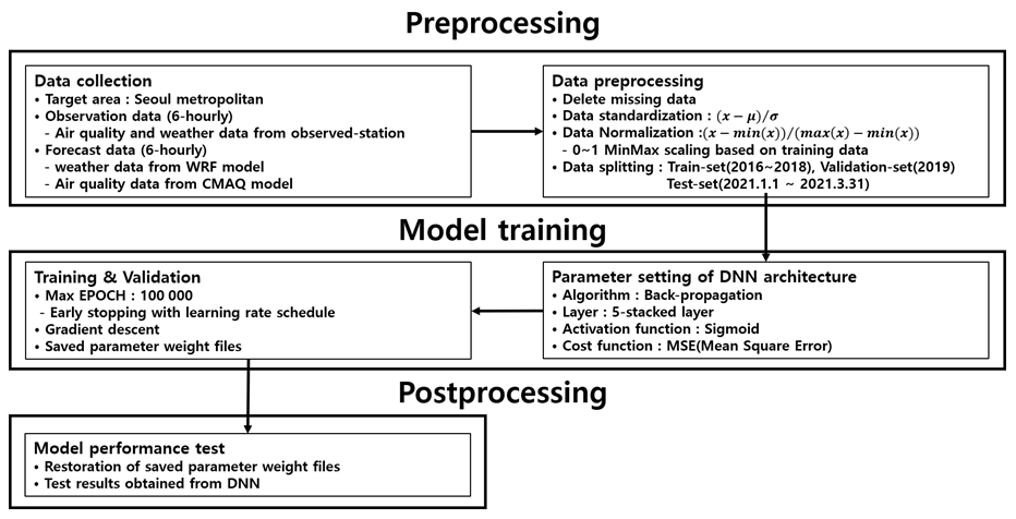
Figure 1 outlines the process for the development of the DNN model used herein, which consists of three broad stages: preprocessing, model training, and post-processing. In the preprocessing stage, the data necessary for the development of the DNN model are collected, and the collected data are processed into a suitable format for use as the training and validation data. In the model training stage, the backpropagation algorithm and parameters are applied to implement the DNN model, and the most optimal “weight file” is saved once training and validation are completed. In the post-processing stage, prediction is performed using the saved “weight file”. Section 2.1 provides a detailed description of the data used for training, and Sect. 2.2 describes the development of the DNN model.

Figure 1 Flowchart of the PM_2.5 forecasting system based on the DNN algorithm.

2.1 Training data acquisition

For training of the DNN model, validating the trained DNN model, and making predictions using the developed DNN model, we used observation data, such as ground-based air quality and weather data, as well as forecasting data, such as ground-based and altitude-specific weather data and ground-based PM_2.5, generated via the WRF and CMAQ models in Seoul, South Korea. In addition, the membership function was used to reflect temporal information. Data pertaining to a 3-year period (2016–2018) were used for training the model, and data pertaining to 2019 were used for validation. Data pertaining to a 3-month period (January to March 2021) were used to evaluate the prediction performance.

Figure 2 illustrates the spatial distribution of the weather and air quality observation points in Seoul, South Korea, where the observation data used for training the model had been measured, and Table 1 presents a list of the weather and air quality observation data variables used for the training. Six variables of air quality (SO₂, NO₂, O₃, CO, PM₁₀, and PM_2.5), measured with the measuring equipment provided by Air Korea on their website, were used to obtain observation data. SO₂ and NO₂ are the precursors that directly affect the changes in the PM_2.5 concentration. O₃ is generated by NO_x and volatile organic compounds (VOCs) and causes direct and indirect effects on the changes in the PM_2.5 concentration (Wu et al., 2017; Geng et al., 2019). CO affects the generation of O₃ in the oxidation process via the OH reaction, which, in turn, has an indirect effect on the changes in the PM_2.5 concentration (Kim et al., 2016). Furthermore, particulate matter with particles exhibiting a less than 10 µm diameter (PM₁₀) is highly correlated with PM_2.5 during periods of high concentration and exhibits similar trends in seasonal concentrations (Mohammed et al., 2017; Gao and Ji, 2018).

Table 1 Training variables in the PM_2.5 prediction system using a DNN based on surface-weather observations. Air quality variables were obtained from 41 air quality measurement equipment in Seoul. Surface weather variables were obtained from ASOS in Seoul. Observation data were collected every hour.

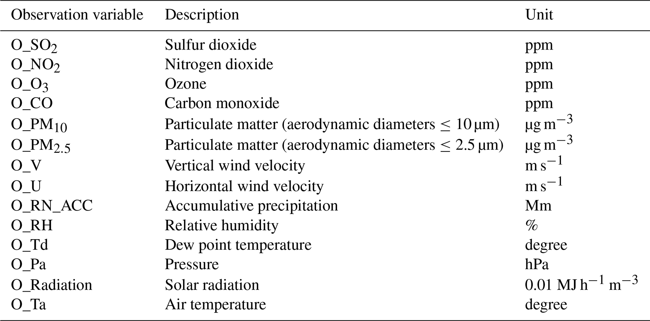
Real-time data from the Automated Surface Observing System (ASOS) were used as the weather data, through the uniform resource locator–application programming interface (URL–API) operated by the Korea Meteorological Administration. The eight variables for the surface-weather data included: vertical and horizontal wind speed, precipitation, relative humidity, dew point, atmospheric pressure, solar radiation, and temperature. Wind speeds and precipitation are known to be negatively correlated with the PM_2.5 concentration, whereas an increase in the relative humidity increases the PM_2.5 concentration. Wind speed is generally associated with turbulence, and an increase in the intensity of the turbulence facilitates the mixing of air, inducing a decrease in the PM_2.5 concentration (Yoo et al., 2020). Precipitation affects the PM_2.5 concentration owing to the washing effect therein. A lower than 80 % increase in the relative humidity affects the increase in the PM_2.5 concentration, owing to increased condensation and nucleation (Yoo et al., 2020; Kim et al., 2020). The dew point is associated with relative humidity; therefore, it has an indirect effect on the PM_2.5 concentration. In addition, atmospheric pressure, solar radiation, and temperature affect the occurrence of high PM_2.5 concentrations and seasonal changes in PM_2.5. In terms of atmospheric pressure, the atmospheric stagnation caused by high pressure influences the occurrence of high PM_2.5 concentrations (Park and Yu, 2018). Solar radiation appears to be negatively correlated with the PM_2.5 concentration in winter (Turnock et al., 2015), and temperature is reported to affect the changes in the PM_2.5 concentration owing to an increased sulfate concentration and decreased nitrate concentration at high temperatures (Dawson et al., 2007; Jacob and Winner, 2009).

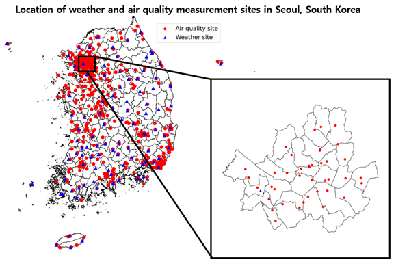
Figure 2 Spatial distributions of weather (▴) and air quality (•) measurement sites in Seoul.

Figure 3 depicts the nested-grid modeling domains used to generate the forecast data in terms of surface-level and altitudinal weather and air quality that is used for training the DNN model, with northeastern Asia represented as Domain 1 (27 km) and the Korean Peninsula represented as Domain 2 (9 km). The simulation results of the Weather Research and Forecasting (WRF, v3.3) model, a regional-scale weather model developed by the National Center for Environmental Prediction (NCEP) under the National Oceanic and Atmospheric Administration (NOAA) in the United States, were used as the weather forecast data. The simulation results obtained via the CMAQ system (v4.7.1) developed by the U.S. Environmental Protection Agency were used as the PM_2.5 prediction data. The unified model (UM) global forecast data provided by the Korea Meteorological Administration were used as the initial and boundary conditions of the WRF model for the weather simulation. In the WRF model simulation, the Yonsei University Scheme (YSU) (Hong et al., 2006) was used for the planetary boundary layer (PBL) physics, the WRF single-moment class-3 (WSM3) scheme (Hong et al., 1998, 2004) was used for cloud microphysics, and the Kain-Fritsch scheme (Kain, 2004) was used for cloud parameterization. The meteorological field generated was converted into a form of data input to the numerical air quality model using the Meteorology–Chemistry Interface Processor (MCIP, v3.6). The Sparse Matrix Operator Kernel Emission (SMOKE, v3.1) model was applied to the emissions inventory of northeastern Asia (excluding South Korea). The Model Inter-Comparison Study for Asia, Phase 2010 (MICS-Asia; Itahashi et al., 2020) and the Clean Air Policy Support System, 2010 (CAPSS) were applied to the emissions inventory of South Korea. The Model of Emissions of Gases and Aerosols from Nature (MEGAN, v2.0.4) was used to represent natural emissions. In case of the CMAQ model for PM_2.5 concentration simulation, the Statewide Air Pollution Research Center, version 99 (SAPRC-99; Carter et al., 1999) mechanism was used for the chemical mechanism, the fifth-generation CMAQ aerosol module (AERO5; Binkowski et al., 2003) was used for the aerosol mechanism, and the Yamartino scheme for mass-conserving advection (YAMO scheme) (Yamartino, 1993) was used for the advection process. We directly generated the training data using the WRF and CMAQ.

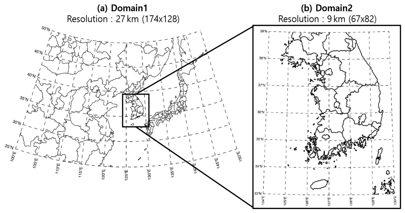
Figure 3 CMAQ modeling domains applied to generate the DNN model training data: (a) Northeastern Asian area with 27 km horizontal grid resolution and (b) Korean Peninsula area with 9 km horizontal grid resolution.

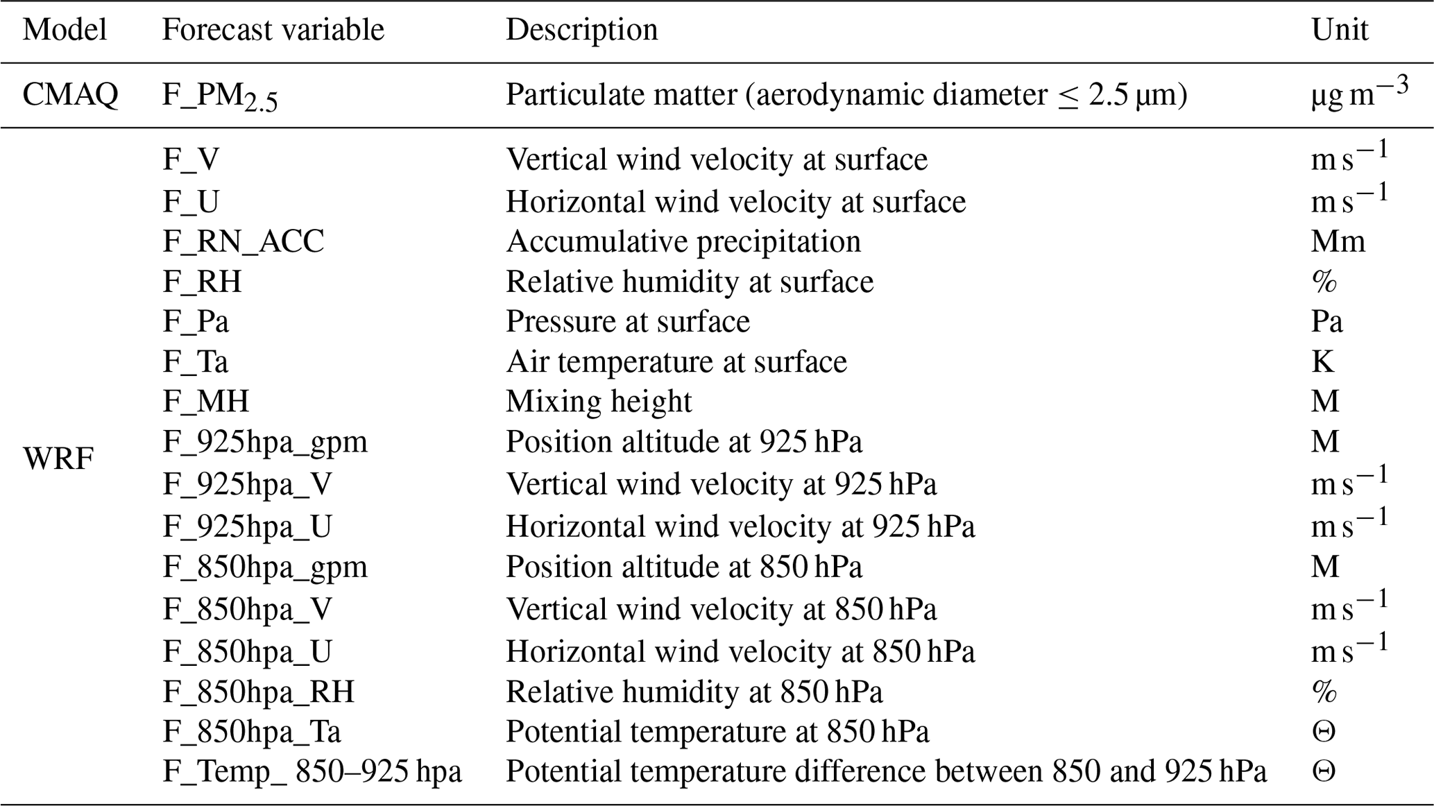
Table 2 presents a list of the weather and air quality prediction model data variables used for training the PM_2.5 prediction system. The air quality forecast variable of the CMAQ model was PM_2.5. Sixteen meteorological forecast variables were created by the WRF model. PM_2.5 and its precursors are emitted from the ground, and they move at an altitude of 1.5 km or less. Therefore, lower altitude data variables were mainly used. The meteorological forecast variables on the ground included vertical and horizontal wind speed, precipitation, relative humidity, atmospheric pressure, temperature, and mixing height. In addition, the predicted meteorological variables for each altitude included the geopotential height as well as the vertical and horizontal wind speed at 925 hPa. The geopotential height, vertical and horizontal wind speed, relative humidity, potential temperature at 850 hPa, and the difference in the potential temperature between 850 and 925 hPa were also included. An increase or decrease in mixing height, which depends on thermal and mechanical turbulence, affects the spread of air pollutants. As the mixing height increases, the diffusion intensity increases and the concentration of air pollutants, such as PM_2.5, decreases. The potential temperature is an indicator of the vertical stability of the atmosphere, and the vertical stability can be used to identify the formation of the inversion layer, which has a significant effect on the PM_2.5 concentration (Wang et al., 2014). Finally, altitude data are associated with the atmospheric stability and long-term transport of air pollutants (Lee et al., 2018).

Table 2 Training variables in the PM_2.5 prediction system using a DNN based on the WRF and CMAQ models. WRF and CMAQ model results were obtained from 9 km horizontal grid resolution. These values were collected on an hourly interval.

To train the DNN model to understand the change patterns in the PM_2.5 concentration over time and consider the propagation of temporal change, time data were generated using the membership function presented by Yu et al. (2019). The concept of the membership function is derived from the fuzzy theory, and it defines the probability that a single element belongs to a set. In this study, the probability that the date (element) belongs to 12 months (set) was calculated using the membership function. PM_2.5 concentration in Seoul is high in January, February, March, and December, and low from August to October. PM_2.5 concentration has a characteristic that changes gradually from month to month. The membership function was used to reflect these monthly change characteristics. The temporal data using the membership function contained 12 variables, representing the months from January to December. The sum of the variables was set to 1. Of the 12 variables, 10 had a value of 0, and 2 had values between 0 and 1. The 2 non-zero variables were determined based on the day of generation of the temporal data and were defined as “month” and “adjacent month”. If the temporal data were generated between the 1st and the 14th day of a “month”, the “adjacent month” referred to the month preceding this “month”. If the temporal data were generated between the 16th to the 31st day of a “month”, the “adjacent month” referred to the month succeeding this “month”. The “adjacent month” was not considered when the temporal data were generated on the 15th day of the “month”. The values of the “adjacent month” and “month” variables were calculated through Eqs. (1)–(4). For example, when generating the temporal data for 10 January, the “month” would be January, and the “adjacent month” would be December. Based on the calculations in Eq. (1), the “month” variable value would equal 0.82 and the “adjacent month” variable value would equal 0.18, and the rest of the variable values from February to November would equal 0:

$$\begin{array}{}\text{(1)}& {\displaystyle }\text{if }\left(d<\mathrm{15}\right)\text{ then “Month value”}={\displaystyle \frac{\mathrm{1}}{\mathrm{28}}}\times d+{\displaystyle \frac{\mathrm{13}}{\mathrm{28}}};\text{(2)}& {\displaystyle }\text{if }\left(d>\mathrm{15}\right)\text{ then “Month value”}=-{\displaystyle \frac{\mathrm{1}}{\mathrm{30}}}\times d+{\displaystyle \frac{\mathrm{3}}{\mathrm{2}}};\text{(3)}& {\displaystyle }\text{if }\left(d=\mathrm{15}\right)\text{ then “Month value”}=\mathrm{1};\text{(4)}& {\displaystyle }\text{and “Adjacent Month value”}=\mathrm{1}-\text{“Month value”}.\end{array}$$

2.2 Implementation of the DNN model

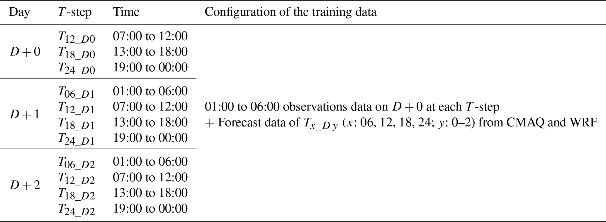
To develop DNN models over 6 h intervals, time steps (T-steps) were constructed for the target period of 3 d (D+0 to D+2) to perform predictions as shown in Table 3. T_{12_D0} to T_{24_D0} are included in the day of prediction (D+0), T_{06_D1} to T_{24_D1} in the 1 d after of prediction (D+1), and T_{06_D2} to T_{24_D2} in the 2 d after of prediction (D+2). Weather and air quality prediction data used in each T-step training data averages 1 h interval data into 6 h interval data; and the 9 km grids corresponding to Seoul were averaged spatially. The observation data used in each T-step training data averages the preceding 6 h period at the beginning of the forecast (01:00 to 06:00 on D+0).

Table 3 Configuration of the training data for each T-step to implement the DNN model for the 6 h average prediction.

The feature scaling, including standardization and normalization, was implemented to transform data into uniform formats, reduce data bias of training data, and ensure equal training for the DNN model at each T-step. The normal distribution of the variables in the training data was standardized through standardization. The variables in the training data were standardized to be distributed in the range of a mean of 0 and standard deviation of 1. The standardized variables of the training data were subsequently normalized to the minimum (min_(x)) and maximum (max_(x)) values so that the values would be bounded in an equal range between 0 and 1. Both normalization and standardization were applied to train the characteristics of training variables equally to the DNN model. Standardization and normalization were performed using the Z-score (Eq. 5) and Min–max scaler (Eq. 6), respectively:

$$\begin{array}{}\text{(5)}& {\displaystyle }Z\mathrm{score}={\displaystyle \frac{x-\mathit{\mu }}{\mathit{\sigma }}};\text{(6)}& {\displaystyle }\text{Min–max scaler}={\displaystyle \frac{x-{\min }_{\left(x\right)}}{{max}_{\left(x\right)}-{\min }_{\left(x\right)}}}.\end{array}$$

Figure 4 depicts the training process of the DNN model. After feature scaling, the training data is trained through the backpropagation algorithm in the five-stacked-layer DNN model. The statistical and AQI performance results of the DNN model based on the layer are presented in Tables S1 and S2, respectively, in the Supplement. The results of the four-stacked-layer and five-stacked-layer models show that the performance is similar. However, compared with the four-stacked-layer model, the RMSE of the five-stacked-layer decreases by approximately 0.1–1 µg m⁻³ at D+0 to D+2, and the ACC of the five-stacked-layer model increases by approximately 1 %p to 6 %p at D+0 to D+2. Therefore, the five-stacked-layer model shows the better performance. The six-stacked-layer and eight-stacked-layer models contain errors that converge without decreasing during the training process of the model (vanishing gradient problem). The cause of this problem is the activate function. The backpropagation algorithm consists of the feedforward and backpropagation processes. Feedforward is the process of calculating the difference (cost) between the output value (hypothesis) and target value (true value) in the output layer, after the calculation has proceeded from the input layer to subsequent layers and finally reached the output layer. Backpropagation is the process of creating new node values for the input layer by updating the weight using the cost calculated in the feedforward process.

In the feedforward process, the node (i) value ($x_i^{\left(l\right)}$) of the previous layer (l) is converted to the hypothesized ($x_i^{(l+\mathrm{1})}$), and the node (m) value of the subsequent layer (l+1) is converted through the weight ($w_{m,i}^l$), deviation (b_m), and sigmoid function ($\mathrm{\varnothing }\left(Z_m^{(l+\mathrm{1})}\right)$), which is an activation function. Equations (7) and (8) outline the calculation process:

$$\begin{array}{}\text{(7)}& {\displaystyle }{Z}_m^{(l+\mathrm{1})}=\sum _{i=\mathrm{1}}^n\left(x_i^{\left(l\right)}\times w_{m,i}^{\left(l\right)}+b_m\right);\text{(8)}& {\displaystyle }{x}_m^{(l+\mathrm{1})}=\mathrm{\varnothing }\left(Z_m^{\left(l+\mathrm{1}\right)}\right)={\displaystyle \frac{\mathrm{1}}{\mathrm{1}+e^{(-Z_m^{(l+\mathrm{1})})}}}.\end{array}$$

The mean squared error (MSE), a cost function, is applied to the difference (cost) between the hypothesized and target value calculated during the forward propagation process, as denoted by Eq. (9) (Hinton and Salakhutdinov, 2006):

$$\begin{array}{}\text{(9)}& \begin{array}{rl}\text{Cost}& ={\displaystyle \frac{\mathrm{1}}{n}}{\left(x_m^{\mathrm{Outlayer}}-\mathrm{Target}\right)}^{\mathrm{2}}\\ & ={\displaystyle \frac{\mathrm{1}}{n}}{\left(\text{Hypothesis}-\text{Target}\right)}^{\mathrm{2}}.\end{array}\end{array}$$

In the backpropagation process, the weights calculated in the feedforward process are updated via the gradient descent method. For weight updating, the corresponding magnitude can be adjusted by multiplying it with a scalar value known as the learning rate (η) (Eq. 10) (Bridle, 1989):

$$\begin{array}{}\text{(10)}& W_{m,i}^{\left(l\right)}=W_{m,i}^{\left(l\right)}-\mathit{\eta }{\displaystyle \frac{\partial \text{Cost}}{\partial W_{m,i}^{\left(l\right)}}}.\end{array}$$

Therefore, the backpropagation algorithm is configured as expressed in Eqs. (5)–(10), and the DNN model learns the features of the training data by repeating the backpropagation algorithm as many times as the number of epochs.

Figure 4 Structure of DNN model training process.

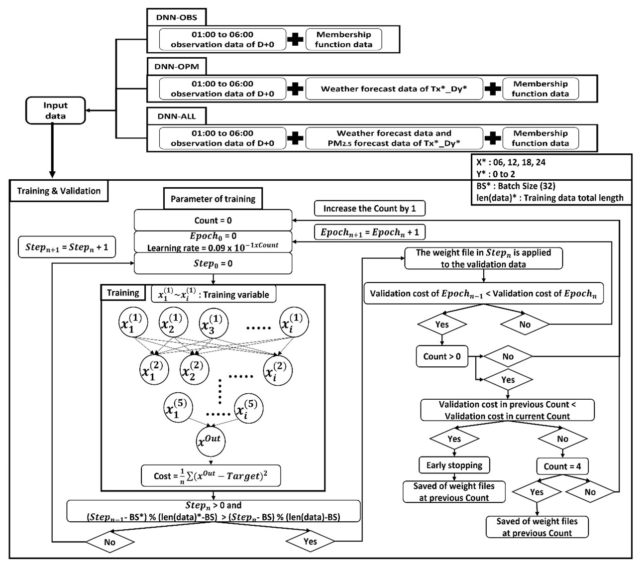
In this study, early-stopping was applied to avoid the overfitting that occurred in the form of a decrease in the cost of the training data while the cost of the validation data increased with the number of epochs. The early-stopping condition is applicable when the cost value of the validation data at Epoch_n is lower than the cost of the validation data from Epoch_n+1 to Epoch_Max. When the early-stopping condition is satisfied, the user-defined variable “Count” increases by 1 if the “Count” is zero, and if “Count” is non-zero, the learning rate decreases by ${\mathrm{10}}^{-\mathrm{1}\times \mathrm{Count}}$, so that learning is performed with an updated learning rate from Epoch_n+1 onwards. When the cost values of the validation data from Epoch_n+1 to Epoch_Max exceed the cost values of Epoch_n in the previous “Count”, the learning of the model is completed.

3 Experimental design and indicators for prediction performance evaluation

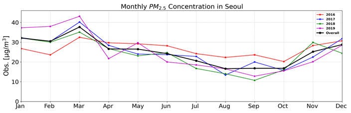
Figure 5 displays the average monthly PM_2.5 concentrations observed in Seoul from 2016 to 2019. The highest average monthly PM_2.5 concentration between 2017 and 2019 was observed in January, March, and December, i.e., during the winter season. The average monthly PM_2.5 concentration ranged between 28.8 and 37.8 µg m⁻³ in winter and 16.6 and 26.6 µg m⁻³ in summer over the 4-year period (2016–2019). This indicated that the concentration in winter exceeded that in summer by approximately 12 µg m⁻³. In this study, the prediction performance of the DNN model was evaluated during winter months (1 January to 31 March 2021) that exhibited high PM_2.5 concentrations.

Figure 5 Time series of the monthly average PM_2.5 concentrations from 2016 to 2019.

Three experiments (DNN-OBS, DNN-OPM, and DNN-ALL) were performed to examine the effects of the training-data configuration on the prediction performance of the DNN model. The DNN-OBS model used the observation data as the sole training data, the DNN-OPM model used both observation and weather forecast data for T_{x_D y} (x: 06, 12, 18, 24; y: 0–2) as the training data, and the DNN-ALL model used the observation data, weather forecast data, and PM_2.5 concentration prediction data T_{x_D y} (x: 06, 12, 18, 24; y: 0–2) as the training data. The observation variables presented in Table 1 in Sect. 2.1 were used as common variables in the three experiments. Among the predictors shown in Table 2 in Sect. 2.1, the variables produced in the WRF model were used in the DNN-OPM and DNN-ALL models, whereas the variables produced in the CMAQ model were used only in the DNN-ALL model.

The prediction performances of the three DNN-model experiments were evaluated based on statistics and the AQI. The MSE, RMSE, IOA, and correlation coefficient (R) were used as the indicators in statistical evaluation. The MSE and RMSE, which represented the loss functions of the DNN model, were used to determine the quantitative difference between the model predictions and observed values. The IOA indicator determined the level of agreement between the model predictions and observed values based on the ratio of the MSE to the potential error. The R indicator determined the correlation between the model predictions and observed values. Equations (11)–(14) were used to calculate these five indicators:

$$\begin{array}{}\text{(11)}& {\displaystyle }\mathrm{MSE}{\left(\mathrm{\mu }\mathrm{g}{\mathrm{m}}^{-\mathrm{3}}\right)}^{\mathrm{2}}={\displaystyle \frac{\mathrm{1}}{N}}\sum _{\mathrm{1}}^N{\left(\mathrm{Model}-\mathrm{Obs}\right)}^{\mathrm{2}};\text{(12)}& {\displaystyle }\mathrm{RMSE}\left(\mathrm{\mu }\mathrm{g}{\mathrm{m}}^{-\mathrm{3}}\right)=\sqrt{{\displaystyle \frac{\mathrm{1}}{N}}\sum _{\mathrm{1}}^N{\left(\mathrm{Model}-\mathrm{Obs}\right)}^{\mathrm{2}}};\text{(13)}& {\displaystyle }\mathrm{IOA}=\mathrm{1}-{\displaystyle \frac{\sum _{\mathrm{1}}^N{\left(\mathrm{Model}-\mathrm{Obs}\right)}^{\mathrm{2}}}{\sum _{\mathrm{1}}^N{\left(\left|\mathrm{Model}-\stackrel{\mathrm{‾}}{\mathrm{Obs}}\right|+\left|\mathrm{Obs}-\stackrel{\mathrm{‾}}{\mathrm{Obs}}\right|\right)}^{\mathrm{2}}}};\text{(14)}& {\displaystyle }R={\displaystyle \frac{\sum \left(\mathrm{Model}-\stackrel{\mathrm{‾}}{\mathrm{Model}}\right)\times \left(\mathrm{Obs}-\stackrel{\mathrm{‾}}{\mathrm{Obs}}\right)}{\sqrt{\sum {\left(\mathrm{Model}-\stackrel{\mathrm{‾}}{\mathrm{Model}}\right)}^{\mathrm{2}}\times \sum {\left(\mathrm{Obs}-\stackrel{\mathrm{‾}}{\mathrm{Obs}}\right)}^{\mathrm{2}}}}}.\end{array}$$

The AQI for PM_2.5 was classified into four categories based on the PM_2.5-concentration standards used in South Korea. PM_2.5 concentrations from 0 to 15 µg m⁻³ were classified as “good”; 16 to 35 µg m⁻³, “moderate”; 36 to 75 µg m⁻³, “bad”; and 76 µg m⁻³ or higher, “very bad”. The ACC determined the categorical prediction accuracy of the model pertaining to the four AQI categories, and the probability of detection (POD) determined the prediction performance of the model for high PM_2.5 concentrations (“bad” and “very bad” AQI categories). The FAR determined the rate of incorrect predictions when the observations tended to be “moderate” or “good”, but the predictions pointed to high concentrations (“bad” or “very bad” AQI categories). A low FAR value indicated better performance. The F1-score indicator, which is the harmonic mean of the POD and FAR, reflected the POD as well as FAR evaluations. Additionally, the recall and precision were evaluated for four categories. The recall is an indicator of how well the model reproduced the categories that appear in observation. The precision is the accuracy that matches the category of observation among the prediction results of the model for each category. Equations (S1)–(S8) in the Supplement were used for calculating the recall and precision. Equations (15)–(18) were used for calculating the AQI prediction-evaluation indicators:

$$\begin{array}{}\text{(15)}& {\displaystyle }\mathrm{ACC}\left(\mathit{\%}\right)={\displaystyle \frac{\left(a\mathrm{1}+b\mathrm{2}+c\mathrm{3}+d\mathrm{4}\right)}{N}}\times \mathrm{100};\text{(16)}& {\displaystyle }\begin{array}{rl}& \mathrm{POD}\left(\mathit{\%}\right)\\ & ={\displaystyle \frac{\left(c\mathrm{3}+c\mathrm{4}+d\mathrm{3}+d\mathrm{4}\right)}{\left(a\mathrm{3}+a\mathrm{4}+b\mathrm{3}+b\mathrm{4}+c\mathrm{3}+c\mathrm{4}+d\mathrm{3}+d\mathrm{4}\right)}}\times \mathrm{100}\end{array};\text{(17)}& {\displaystyle }\begin{array}{rl}& \mathrm{FAR}\left(\mathit{\%}\right)\\ & ={\displaystyle \frac{(c\mathrm{1}+c\mathrm{2}+d\mathrm{1}+d\mathrm{2})}{(c\mathrm{1}+c\mathrm{2}+c\mathrm{3}+c\mathrm{4}+d\mathrm{1}+d\mathrm{2}+d\mathrm{3}+d\mathrm{4})}}\times \mathrm{100}\end{array};\text{(18)}& {\displaystyle }\mathrm{F}\mathrm{1}\mathrm{score}=\mathrm{2}\times {\displaystyle \frac{\mathrm{POD}\times (\mathrm{100}-\mathrm{FAR})}{\mathrm{POD}+(\mathrm{100}-\mathrm{FAR})}}.\end{array}$$

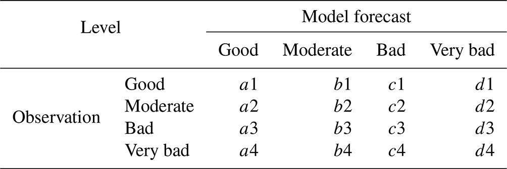
Table 4 lists the intervals corresponding to the four categories for calculating ACC, POD, FAR, and recall and precision.

Table 4 Intervals corresponding to the four categories for calculating ACC, POD, FAR, and recall and precision: “good” (PM_2.5≤15 µg m⁻³); “moderate” (16 µg m${}^{-\mathrm{3}}\le$ PM_2.5≤35 µg m⁻³); “bad” (36 µg m${}^{-\mathrm{3}}\le$ PM_2.5≤75 µg m⁻³); and “very bad” (76 µg m${}^{-\mathrm{3}}\le$ PM_2.5).

The effect of the training data on the prediction performance of the DNN model was quantitatively analyzed using the RMSE indicator. The overall effect of the forecast data on model predictions was calculated based on the RMSE difference between the DNN-ALL and DNN-OBS models. The effect of the predicted weather data on model predictions was calculated based on the RMSE difference between the DNN-OPM and DNN-OBS models (Eq. 19):

$$\begin{array}{}\text{(19)}& {\displaystyle }\begin{array}{rl}& \text{Contribution of predicted weather }\left(\mathit{\%}\right)\\ & =\left|{\displaystyle \frac{\left(\mathrm{DNN}-{\mathrm{OPM}}_{D+i}\right)-\left(\mathrm{DNN}-{\mathrm{OBS}}_{D+i}\right)}{\left(\mathrm{DNN}-{\mathrm{ALL}}_{D+i}\right)-\left(\mathrm{DNN}-{\mathrm{OBS}}_{D+i}\right)}}\right|\\ & \times \mathrm{100}\left(i=\mathrm{0}\text{–}\mathrm{2}\right).\end{array}\end{array}$$

The effect of the predicted PM_2.5 data on model predictions was calculated based on the RMSE difference between the DNN-ALL and DNN-OBS models (Eq. 20).

$$\begin{array}{}\text{(20)}& {\displaystyle }\begin{array}{rl}& \text{Contribution of predicted }{\mathrm{PM}}_{\mathrm{2.5}}\left(\mathit{\%}\right)\\ & =\left|{\displaystyle \frac{\left(\mathrm{DNN}-{\mathrm{ALL}}_{D+i}\right)-\left(\mathrm{DNN}-{\mathrm{OPM}}_{D+i}\right)}{\left(\mathrm{DNN}-{\mathrm{ALL}}_{D+i}\right)-\left(\mathrm{DNN}-{\mathrm{OBS}}_{D+i}\right)}}\right|\\ & \times \mathrm{100}(i=\mathrm{0}\text{–}\mathrm{2}).\end{array}\end{array}$$

4 Evaluation of prediction performance

The evaluations based on statistics and AQI classifications were conducted for each of the DNN-model experiments (DNN-OBS, DNN-OPM, and DNN-ALL), and the results were compared with those of the CMAQ model currently operational in South Korea. In Sect. 4.1, we examine the daily prediction performance of the three DNN-model experiments and CMAQ model using statistical indicators for the 3 d period (D+0 to D+2), and quantitatively analyze the effect of different training data combinations on the prediction performance of the DNN model. A comparative evaluation with the CMAQ model was conducted to assess whether the DNN-ALL model was more comprehensive for 6 h average forecasting than the existing daily average forecasting model. In Sect. 4.2, to assess the potential of DNN-ALL as a superior forecasting model, the daily AQI predictions therein for the 3 d period (D+0 to D+2) were compared with those of the CMAQ model.

4.1 Evaluation of daily prediction performance based on the training data

Table S3 in the Supplement shows the statistical evaluation results of three DNN-model experiments (DNN-OBS, DNN-OPM, and DNN-ALL) and CMAQ model during the training period from 2016 to 2018. In D+0 to D+2, the DNN-ALL model performs the best in terms of all statistical indicators. In addition, the values of all three experiments indicate a decrease in the RMSE compared to the CMAQ model. Table S4 in the Supplement presents the statistical evaluation results of the three experiments and CMAQ models during the validation period in 2019. The DNN-OBS model shows similar performance for D+0 compared with the CMAQ model but decreased performance owing to an increased RMSE of D+1 and D+2 by 2.0 and 2.2 µg m⁻³, respectively. The DNN-OPM model shows an increase in performance owing to a decrease in the RMSE of D+0 and D+1 by 3.0 µg m⁻³ and 0.4 µg m⁻³, respectively, compared with the CMAQ model, indicating that the performance is similar. However, the RMSE of D+2 increased by 0.4 µg m⁻³ compared with the CMAQ model. For the DNN-ALL model, the RMSE from D+0 to D+2 decreased by 4.6, 2.7, and 2.1 µg m⁻³, compared with the CMAQ model, which shows an improved performance.

Table 5 Statistical summary of daily PM_2.5 concentration prediction performance of the CMAQ, DNN-OBS, DNN-OPM, and DNN-ALL models.

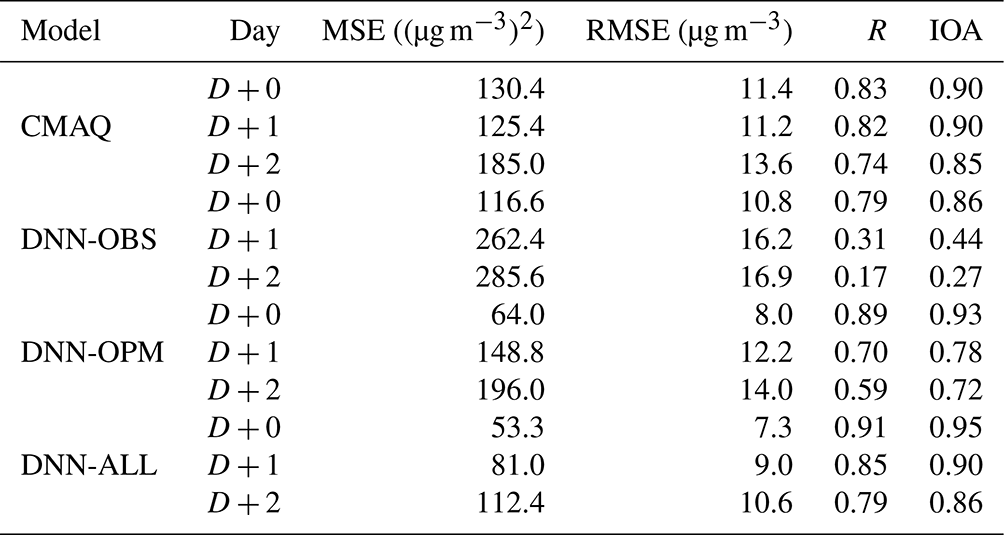
Table 5 summarizes the results of the statistical evaluations of the prediction performances of the three DNN-model experiments and the CMAQ model in the test set (January to March 2021). Figure 6 depicts the corresponding Taylor diagrams, and Fig. 7 illustrates the corresponding time series. For D+0, the CMAQ model RMSE was 11.4 µg m⁻³ with a 0.90 IOA, and that of the DNN-OBS was 10.8 µg m⁻³ with a 0.86 IOA, thereby indicating a lower error and IOA compared with those of the CMAQ model. The RMSEs of the DNN-OPM and DNN-ALL were 8.0 and 7.3 µg m⁻³, respectively, and their IOAs were 0.93 and 0.95, respectively, indicating decreased errors and increased IOAs compared with those of the CMAQ model. Based on the RMSE and IOA values, the DNN-ALL exhibited the best prediction performance. The Taylor diagram (Fig. 6a), which depicts the RMSE, R, and standard deviation indicators simultaneously, confirms that DNN-ALL demonstrated the best prediction performance among the evaluated models. Figure 7a1 and a2 reveal that all three of the DNN-model experiments exhibited improved overprediction performance compared with the CMAQ model; however, the DNN-OBS exhibited the highest underprediction of PM_2.5 concentration during the high-concentration period (11–14 February). The domestic and foreign contributions to the high-concentration period were analyzed using the CMAQ with the brute-force method (CMAQ-BFM) model (Bartnicki, 1999; Nam et al., 2019). The BFM revealed that the foreign contribution to the PM_2.5 concentration because of the long-term transport of pollutants to the Seoul area was 68 % on 11 February, 54 % on 12 February, 66 % on 13 February, and 41 % on 14 February. This aspect of the high PM_2.5 concentration could not be characterized solely by using observation data (data observed at each point) as the training data. This phenomenon seemed to cause an increase in the concentration on the day subsequent to the day a high concentration occurred. The DNN-OBS RMSE obtained on excluding the high-concentration period was 9.4 µg m⁻³, which was lower than that of the CMAQ model (10.9 µg m⁻³) and 1.4 µg m⁻³ lower than that exhibited by the DNN-OBS model when the high-concentration period was included. In contrast, the RMSEs of the DNN-OPM and DNN-ALL were 7.3 and 7.0 µg m⁻³, respectively, the IOAs were 0.93 and 0.94, respectively, and the R values were 0.89 for both models, when the high-concentration period was excluded. No significant difference in results was observed even on inclusion of the high-concentration period (11–14 February). These results suggest that when the observation and prediction data are used as the training data, the DNN model reflects the characteristics of the high-concentration phenomenon caused by long-distance transport. Excluding the high PM_2.5 concentration caused by long-term transport, the DNN model demonstrated a marginally improved prediction performance compared with the CMAQ model on D+0, even when using only the observation data as the training data. In addition, the use of the prediction data as the training data facilitated an improved prediction performance concerning the long-term-transport-induced phenomenon compared with that of the CMAQ model.

For D+1 and D+2, the CMAQ model RMSEs were 11.2 and 13.6 µg m⁻³, respectively, and the IOAs were 0.90 and 0.85, respectively. In contrast, the DNN-OBS RMSEs for D+1 and D+2 were 16.2 and 16.9 µg m⁻³, respectively, and the IOAs were 0.44 and 0.27, respectively. Thus, the DNN-OBS model resulted in larger errors and smaller IOAs compared with the CMAQ model. The errors increased and the IOAs decreased for the DNN-OPM, when compared with those of the CMAQ model. However, the DNN-OPM model RMSEs decreased by 4.0 and 2.9 µg m⁻³, and the IOAs increased by 0.34 and 0.45 compared with those of the DNN-OBS model, for D+1 and D+2, respectively. The DNN-ALL model performed the best, with RMSEs of 9.0 and 10.6 µg m⁻³ and IOAs of 0.90 and 0.86 for D+1 and D+2, respectively, exhibiting smaller errors and larger IOAs compared with those of the CMAQ model. The standard deviations of the DNN-ALL model were 13.5 and 12.7 µg m⁻³ for D+1 and D+2, respectively. For D+1 and D+2, DNN-ALL outperformed the remaining DNN models and the CMAQ model (Fig. 6b and c). This was concluded based on the superior RMSE and R values exhibited therein. Moreover, as shown in Fig. 7b1, b2, c1, and c2, the DNN-ALL model exhibited lower overprediction compared with that by the CMAQ model. However, the DNN-OBS and DNN-OPM models overpredicted low PM_2.5 concentrations and underpredicted high PM_2.5 concentrations, when compared with the observation data. The DNN-OBS model did not predict the change in the observed PM_2.5 concentration after D+0, indicating a decrease in IOA and a limited range of predicted PM_2.5 concentrations with respect to the observations. Although the DNN-OPM model outperformed DNN-OBS, it was inferior to DNN-ALL because the DNN-OPM training data lacked sufficient features for predicting the change in the observed PM_2.5 concentration. The DNN-ALL model outperformed the CMAQ model for D+1 and D+2, while all three DNN-based models outperformed the CMAQ model for D+0. For D+1 and D+2, the RMSE of the DNN-ALL model decreased by 7.2 and 6.3 µg m⁻³, respectively, compared with DNN-OBS. The effects of weather forecast data were 56 % (4 µg m⁻³) and 46 % (2.9 µg m⁻³), respectively, and those of predicted PM_2.5 concentration were 44 % (3.2 µg m⁻³) and 54 % (3.4 µg m⁻³), respectively, when used as training data. These results suggest that as the prediction period lengthens, the weather forecast and PM_2.5 concentration prediction data are more important than current observation data for improving the model prediction performance.

Also, the performance of the Random Forest (RF) model, one of the statistical models, was evaluated and compared with DNN-ALL. Table S5 in the Supplement shows the statistical evaluation of the Random Forest (RF) model, and the DNN-ALL model with the best results in the statistical evaluation of the three experiments and CMAQ model. Compared with the RF model, the RMSE value of the DNN-ALL model decreased by 0.6–1.9 µg m⁻³, and the R and IOA values increased slightly. Although the volume of training data in this paper was not sufficiently huge to be applied to DNN model, the DNN model outperformed the RF model. In the future, the DNN model can also reflect the expansion of training data and consider the scalability of the model that can predict future data growth over time and segmentation with a 1 h interval. Therefore, the performance of the DNN model is expected to improve as the training data increases.

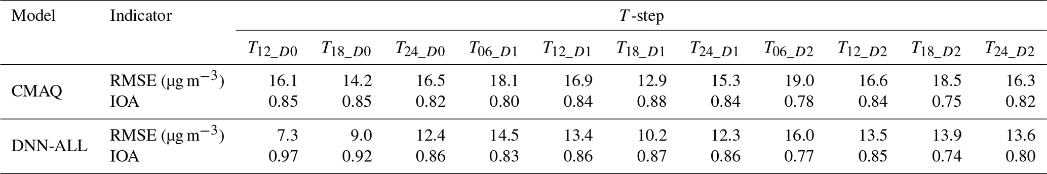
In modern times, people demand the availability of more detailed forecasts, well in advance of the average daily forecast, to enable better planning of daily lives and the mitigation of air-polluting emissions. Therefore, the applicability of the DNN-ALL model as a 6 h forecast model was evaluated. Furthermore, the 6 h mean prediction performance of the DNN-ALL model was evaluated against that of the CMAQ model. Table 6 presents the RMSE and IOA for each T-step of the DNN-ALL and CMAQ models. The RMSEs of the DNN-ALL model ranged between 7.3 and 16.0 µg m⁻³, a decrease of 2.7–8.8 µg m⁻³ compared with the CMAQ model. The DNN-ALL IOAs ranged between 0.74 and 0.97, indicating higher (or similar) IOAs than those of the CMAQ model. However, the RMSE and IOA of the DNN-ALL model did not decrease monotonically. This is because the model performance may differ according to the conditions of target time such as daytime, nighttime, high concentration, and low concentration. As shown in the CMAQ model results, the prediction performance of the DNN-ALL model degrades or improves monotonically over time.

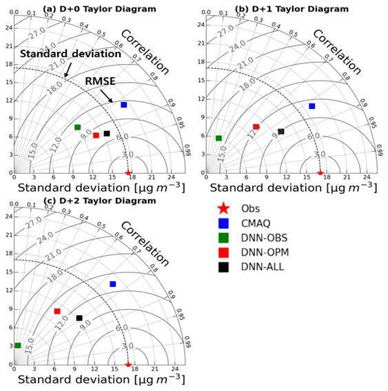
Figure 6 Taylor diagrams for D+0 to D+2 (a–c) of the CMAQ, DNN-OBS, DNN-OPM, and DNN-ALL models. In each diagram, the contour line connecting the x and y axes represents the standard deviation, and the dark gray contour line represents the RMSE. The smaller the RMSE, the higher the R value; the closer the standard deviation is to the standard deviation of the observation, the closer it is to the Obs (⋆).

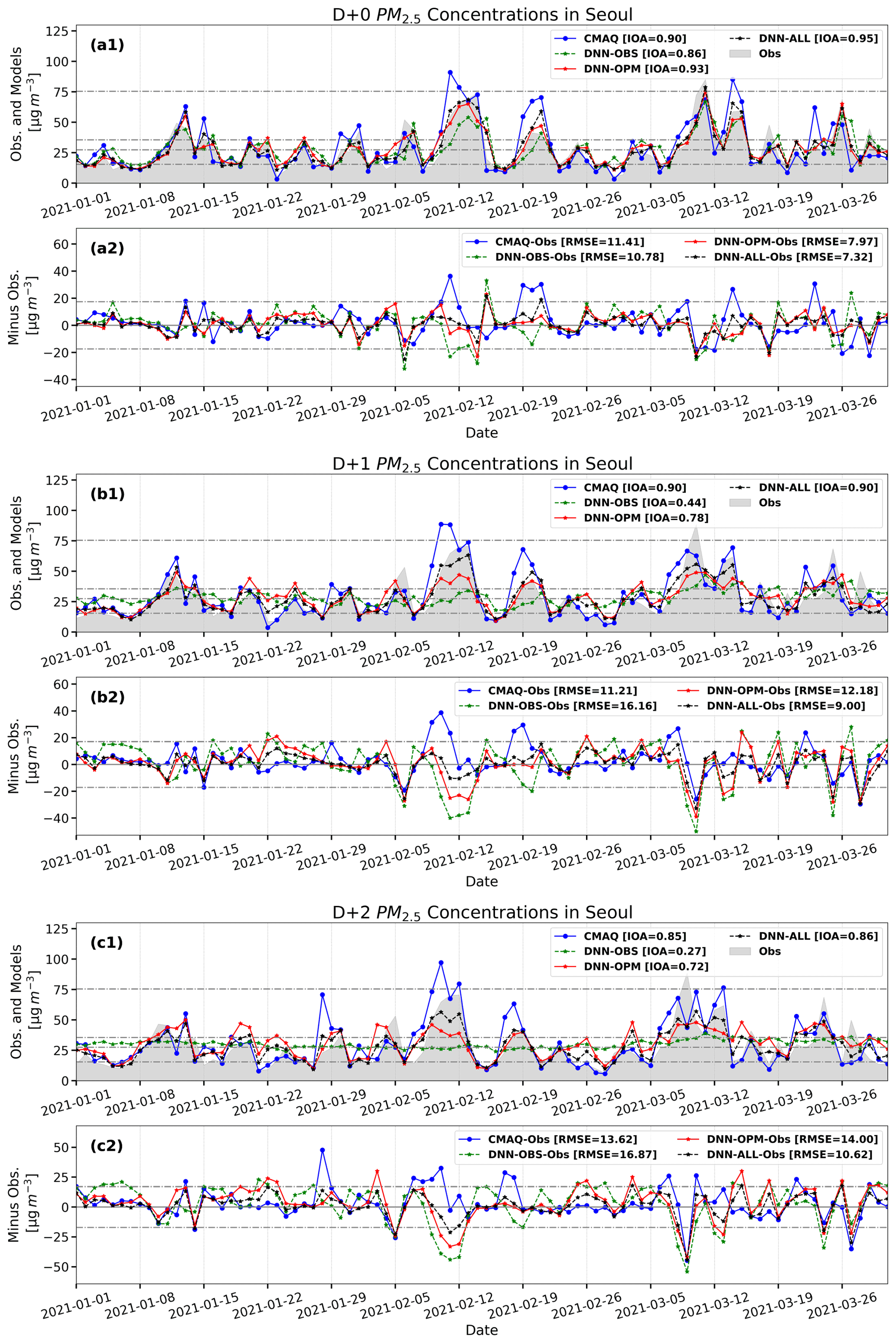
Figure 7 Time series of PM_2.5 concentrations from observations and predictions using the CMAQ, DNN-OBS, DNN-OPM, and DNN-ALL models. Panels (a1)–(c1) depict the time series of predictions and observations and (a2)–(c2) depict the differences between the predictions and observations (predictions minus observations). In (a1)–(c1), each of the dashed lines represents values of 15.5, 35.5, 75.5, and the average value of observation (27 µg m⁻³). In (a2)–(c2), the dashed lines represent the standard deviation of observation PM_2.5 as negative and positive.

Table 6 Statistical summary of the performances of the CMAQ and DNN-ALL models in the case of 6 h average PM_2.5 forecasts.

4.2 AQI-prediction performance

Among the three experiments described in Sect. 4.1, the DNN-ALL model demonstrated the best results in the statistical evaluation. The AQI-prediction performance of the DNN-ALL model was compared with that of the CMAQ and RF model.

Table 7 and Fig. 8 present the AQI evaluation results of the DNN-ALL and CMAQ models. The overall ACC of the DNN-ALL model for D+0 was 77.8 %, 12.2 %p higher than that of the CMAQ model. The categorical-prediction ACC of the DNN-ALL was greater than that of the CMAQ model by 7.4 %p for “good”, 17.1 %p for “moderate”, 4.8 %p for “bad”, and 100 %p for “very bad”. During the target period of this study, “very bad” occurred once. Although DNN-ALL predicted this occurrence accurately, the CMAQ predicted “bad”, indicating a 100 %p difference in accuracy between the two models (Fig. 8a1, b1). The F1 score was 80 %, 3 %p higher than that of the CMAQ model. The FAR of the DNN-ALL model improved by 16.9 %p, although the POD decreased by 9.1 %p. These results suggest that the DNN-ALL model overpredicted less than the CMAQ model, whose predicted PM_2.5 concentrations were generally higher than the observed values.

Table 7 Categorical forecast scores of the performance of the CMAQ and DNN-ALL models.

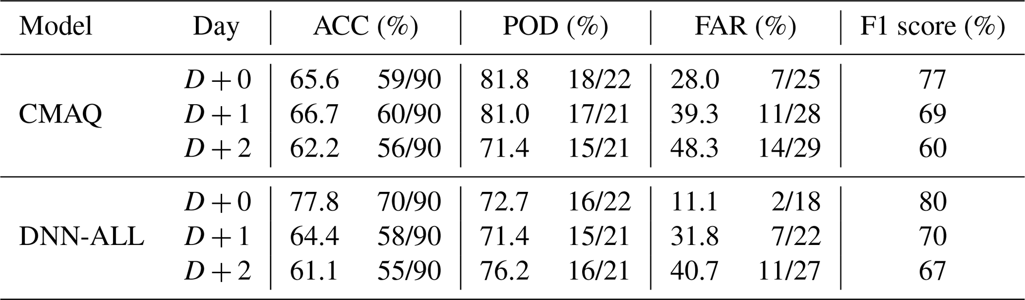
For D+1 and D+2, the overall ACC was 64.4 % and 61.1 %, respectively, a decrease of 2.3 %p and 1.1 %p, respectively, compared with the CMAQ model. The AQI-prediction ACC of the DNN-ALL model decreased by 26.9 %p on both days in “good”, and increased by 11.6 %p for D+1 and 4.7 %p for D+2 in “moderate”. The “good” ACC was low because the CMAQ model underpredicted, and the DNN-ALL model overpredicted, with respect to the observed values. An equal “bad” ACC of 70.0 % was obtained via the DNN-ALL and CMAQ models for D+1, which increased by 20.0 %p for the DNN-ALL model on D+2 (Fig. 8a2, a3, b2, and b3). The F1 score of DNN-ALL model was 70.0 % for D+1 and 67.0 % for D+2; however, the F1 score increased for the DNN-ALL model by 1 %p for D+1 and 7 %p for D+2. For the DNN-ALL model, in the case of D+1, the POD decreased by 9.6 %p and FAR improved by 7.5 %p, whereas in the case of D+2, the POD increased by 4.8 %p and FAR improved by 7.6 %p.

Table S6 in the Supplement shows the precision and recall of all categories for the DNN-ALL and CMAQ models. The precision and recall of the DNN-ALL model in the bad category are presented to be higher than those of the CMAQ model. In the bad category of D+0, the precision and recall of the DNN-ALL model are greater than those of the CMAQ model by 0.24 and 0.04, respectively. In addition, in the “very bad” category, the precision and recall of the DNN-ALL model are to be 1.0 equally higher than those of the CMAQ model. In D+1, the precision of the DNN-ALL model in the “bad” category is greater than that of the CMAQ model by 0.10, but the recall is similar to the CMAQ model. In D+2, the precision and recall for the “bad” category of the DNN-ALL model increased by 0.14 and 0.20 compared with the CMAQ model, respectively. These results show that the performance of the DNN-ALL model is superior to that of the CMAQ model for predicting high concentrations that affect the health of the people.

Table S7 in the Supplement shows the AQI evaluation results of the DNN- ALL and RF models. The ACC of the DNN-ALL model increased by approximately 2 %p– 13 %p compared with the RF model, and the F1 score decreased by 1 %p at D+1 but increased by 1 %p and 9 %p at D+0 and D+2, respectively.

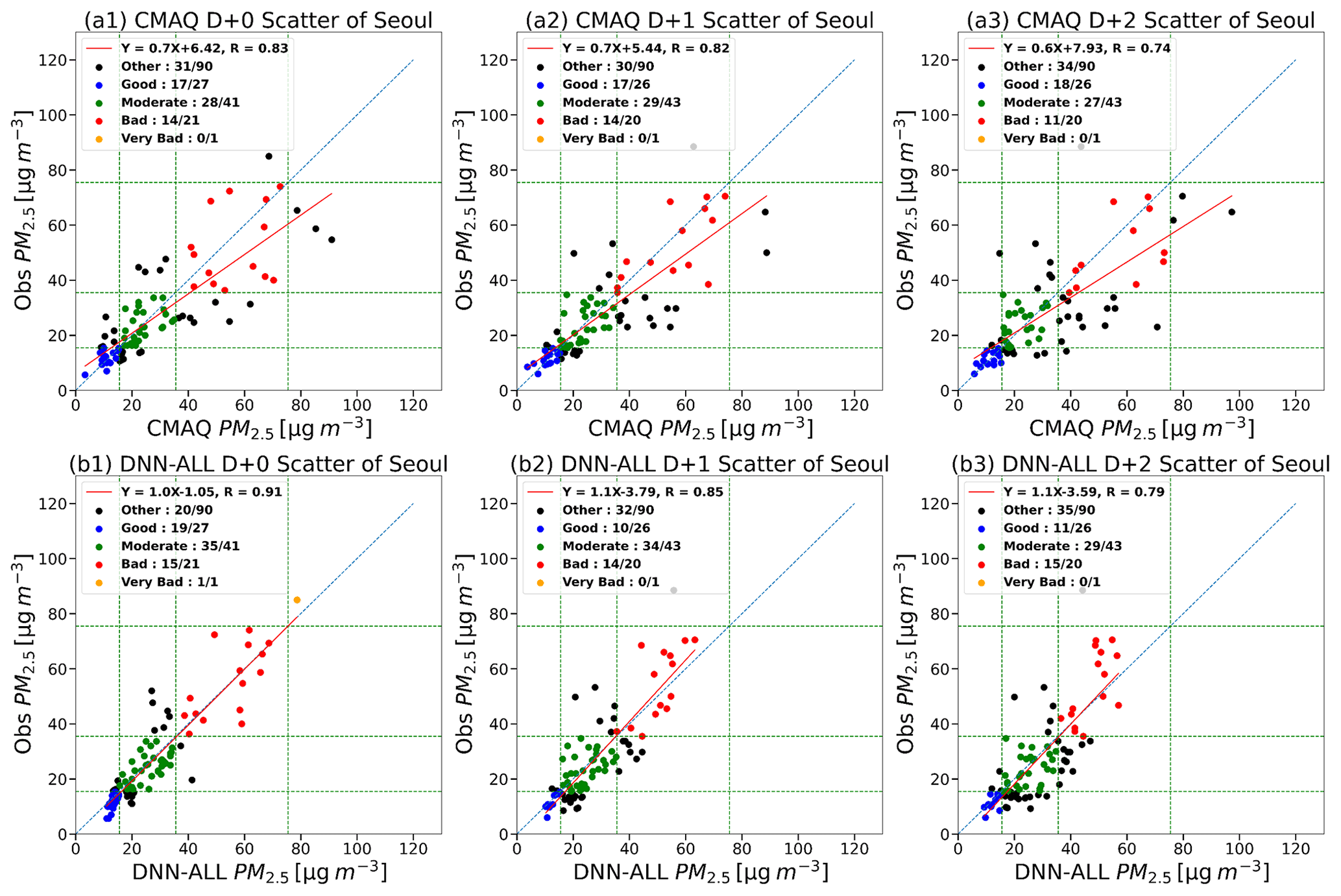
Figure 8 Observations from D+0 to D+2 and corresponding scatter plots of the DNN-ALL and CMAQ models. Panels (a1)–(a3) show the scatter plot of the CMAQ model and observation. Panels (b1)–(b3) show the scatter plot of the DNN-ALL model and observation. The blue dots indicate the observation and prediction values in the AQI category “good”; the green dots, “moderate”; the red dots, “bad”; and the orange dots, “very bad”.

5 Conclusion

The DNN model, a kind of machine learning approach, has been developed for predicting the 6 h average PM_2.5 concentration up to 2 subsequent days (D+0 to D+2) using the observation and forecast data for weather and PM_2.5 concentration to surmount limitations in numerical air quality models such as uncertainties in physical and chemical parameterizations, meteorological data, and emission inventory database. The performance of the DNN model was comparatively evaluated against the currently operational CMAQ model, a kind of numerical air quality model, in South Korea. The effects of different training data on the PM_2.5 prediction of the DNN model were also analyzed.

Compared with the CMAQ model, the RMSE of the DNN-OPM and DNN-OBS models increased by 1.0 and 5.0 µg m⁻³ for D+1, and by 0.4 and 3.3 µg m⁻³ for D+2, even though it decreased by 3.4 and 0.6 µg m⁻³ for D+0, respectively. On the other hand, the RMSE of the DNN-ALL model continued to decrease by 4.1, 2.2, and 3.0 µg m⁻³ for the 3 consecutive days compared to CMAQ model and also decreased by 7.2 µg m⁻³ (D+1) and 6.3 µg m⁻³ (D+2) compared with DNN-OBS model. These results indicated that the use of forecasting data as the training data greatly affected the performance of the DNN model as the forecasting days increased. The RMSE of the DNN-ALL model decreased within a range of 2.7–8.8 µg m⁻³ in the 6 h average PM_2.5 prediction compared with CMAQ model. These results showed that the DNN model outperformed the CMAQ model when it was simultaneously trained by using the observation and forecasting data from the numerical air quality model in both 6 h average and daily forecasting. The DNN-ALL model showed that the F1 score increased by 3 %p, 1 %p, and 7 %p, and FAR decreased by 16.9 %p, 7.5 %p, and 7.6 %p for the 3 consecutive days, indicating that the DNN-ALL model substantially mitigated the overprediction of the CMAQ model in high PM_2.5 concentrations. Our results suggest that the machine learning approach can be a useful tool to overcome limitations in numerical air quality models. For further performance improvement of the DNN model, spatial training data should be expanded to reflect the changes in PM_2.5 concentration induced by the surrounding areas, and the training duration should be increased to allow learning pertaining to the varying concentrations. In addition, the improvement of the numerical models used for generating weather and air quality prediction data is necessary.

When high PM_2.5 concentrations are predicted, mitigation policies are implemented for the protection of public health in South Korea. These policies aim to reduce air-polluting emissions by limiting the power-generation capacity of thermal power plants and operation of vehicles, which are processes that involve socioeconomic costs. Consequently, inaccurate forecasts of high PM_2.5 concentrations can result in socioeconomic losses. Therefore, the use of the DNN model for forecasting is expected to reduce economic losses and protect public health.