the Creative Commons Attribution 4.0 License.
the Creative Commons Attribution 4.0 License.
 | 05 May 2022
An aerosol vertical data assimilation system (NAQPMS-PDAF v1.0): development and application
Haibo Wang
Zifa Wang
Jianjun Li
Wenxuan Chai
Guigang Tang
Xueshun Chen
Aerosol vertical stratification is important for global climate and planetary boundary layer (PBL) stability, and no single method can obtain spatiotemporally continuous vertical profiles. This paper develops an online data assimilation (DA) framework for the Eulerian atmospheric chemistry-transport model (CTM) Nested Air Quality Prediction Model System (NAQPMS) with the Parallel Data Assimilation Framework (PDAF) as the NAQPMS-PDAF for the first time. Online coupling occurs based on a memory-based way with two-level parallelization, and the arrangement of state vectors during the filter is specifically designed. Scaling tests demonstrate that the NAQPMS-PDAF can make efficient use of parallel computational resources for up to 25 000 processors with a weak scaling efficiency of up to 0.7. The 1-month long aerosol extinction coefficient profiles measured by the ground-based lidar and the concurrent hourly surface PM2.5 are solely and simultaneously assimilated to investigate the performance and application of the DA system. The hourly analysis and subsequent 1 h simulation are validated through lidar and surface PM2.5 measurements assimilated and not assimilated. The results show that lidar DA can significantly improve the underestimation of aerosol loading, especially at a height of approximately 400 m in the free-running (FR) experiment, with the mean bias (BIAS) changing from −0.20 (−0.14) km−1 to −0.02 (−0.01) km−1 and correlation coefficients increasing from 0.33 (0.28) to 0.91 (0.53) averaged over sites with measurements assimilated (not assimilated). Compared with the FR experiment, simultaneously assimilating PM2.5 and lidar can have a more consistent pattern of aerosol vertical profiles with a combination of surface PM2.5 and lidar, independent extinction coefficients from the Cloud-Aerosol Lidar with Orthogonal Polarization (CALIOP), and aerosol optical depth (AOD) from the Aerosol Robotic Network (AERONET). Lidar DA has a larger temporal impact than that in PM2.5 DA but has deficiencies in subsequent quantification on the surface PM2.5. The proposed NAQPMS-PDAF has great potential for further research on the impact of aerosol vertical distribution.
- Article
(10679 KB) - Full-text XML
- Companion paper
-
Supplement
(1133 KB) - BibTeX
- EndNote


Aerosol vertical distribution has a significant impact on the estimation of the global budget of aerosols on climate (Torres et al., 1998; Peters et al., 2011; Meyer et al., 2013), planetary boundary layer (PBL) stability (Z. Li et al., 2017; J. Li et al., 2020; Su et al., 2020), the understanding of the aerosol evolutionary process and surface concentration (Chen et al., 2009; Liu et al., 2018; Quan et al., 2020), and the retrieval of aerosol optical properties from passive sensors (C. Li et al., 2020).
In a broad sense, aerosol optical depth (AOD) measurements, which are the vertical integral of aerosol extinction coefficients, can be deemed to include vertical information and have relatively low uncertainty (Holben et al., 2001). However, AOD with passive remote sensors can only be used to investigate the qualitative impact of aerosol vertical distribution (Zhu et al., 2018) and the quantitative relationship with surface concentration, which neglects vertical information to some extent (R. Li et al., 2018; Yang et al., 2019; Wei et al., 2021). Aircraft measurements can directly provide aerosol vertical mass concentration profiles (Bahreini, 2003; Chen et al., 2009; Q. Liu et al., 2019) but are limited in spatiotemporal coverage due to expensive costs at present. Lidar, an effective tool to measure aerosol stratification with active remote sensors, is widely used in vertical research on aerosols (Shimizu, 2004; Liu et al., 2013; Sicard et al., 2015; Proestakis et al., 2019; Mehta et al., 2021) and is generally composed of ground-based and spaceborne lidar. Compared with the relatively large retrieval errors and sparse coverage from satellite observations, ground-based lidar measurements are more accurate (X. Cheng et al., 2019). However, although ground-based lidar generally has more intensive coverage than spaceborne measurements, it can only provide single-point information with limited spatial coverage. The three-dimensional structure of aerosols, especially their vertical structure (Solazzo et al., 2013; Kipling et al., 2016), can be simulated by the atmospheric chemistry-transport model (CTM), which nonetheless has large uncertainties in chemical initial/boundary conditions, meteorological initial/boundary conditions, emissions, and parameterizations of physical and chemical processes (Wu et al., 2020b) and may differ substantially from the real situation.
Currently, there is no single method to obtain spatiotemporally continuous data of aerosol vertical profiles. Therefore, a combination of the advantages of these two approaches can provide more accurate aerosol profiles, which can be done through data assimilation (DA). DA is a technique that combines observations of a system, including their uncertainty, with estimates of that system from a numerical model, including its uncertainty, to obtain a more accurate description of the system including an uncertainty estimate of that description (Evensen, 2009; Vetra-Carvalho et al., 2018). Currently, ensemble Kalman filter (EnKF) (Evensen, 1994)-based methods and three-dimensional/four-dimensional variational methods (3D-/4D-Var) (Schlatter, 2000) are mainstream algorithms. Variational methods are restricted in adequately quantifying the flow-dependent background error and have to program complex adjoint operators (Bannister, 2017). The EnKF, originating from the merger of the traditional Kalman filter (KF) theory (Kalman and Bucy, 1961) and the Monte Carlo estimation methods, uses an ensemble of possible realizations containing valuable flow-independent information (Houtekamer and Zhang, 2016) and has a variety of variants, such as the ensemble square root filter (EnSRF), the local ensemble transform Kalman filter (LETKF) (Bishop and Toth, 1999; Hunt et al., 2007), and the local error-subspace transform Kalman filter (LESTKF) (Nerger et al., 2012). DA has been used in meteorology and oceanography to improve forecasts and construct reanalysis for many decades (Park and Xu, 2009; Lahoz et al., 2010). The application of DA in atmospheric chemistry has only occurred since the mid-1990s (Bocquet et al., 2015) and has mainly involved producing accurate air pollutant concentration analyses and forecasts (Tang et al., 2011; Peng et al., 2017; Ma et al., 2019), improving the inversion of emissions (Tang et al., 2016; Kong et al., 2019; Feng et al., 2020; Wu et al., 2020a), inverting model parameters (Bocquet, 2012), and constructing air quality reanalysis datasets (Lynch et al., 2016; Kong et al., 2021). These common studies mentioned above have mainly concentrated on the performance of assimilating surface measurements in CTMs.
As lidar is the most powerful instrument to measure aerosol vertical information, lidar DA with CTMs has naturally become a popular research area. The study on lidar DA started in 2007, as optimized dust emissions were obtained by assimilating National Institute for Environmental Studies (NIES) lidar measurements during the extreme dust phenomenon on 30 April 2005 (Yumimoto et al., 2007). Since then, a few studies have been conducted on the application of lidar DA: studies on assimilating virtual lidar measurements based on an observing system simulation experiment (OSSE) (Wang et al., 2013), studies on assimilating spaceborne Cloud-Aerosol Lidar with Orthogonal Polarization (CALIOP) (Sekiyama et al., 2010; Zhang et al., 2011; Y. Cheng et al., 2019), studies on investigating the short-term (no more than 12 h) performance of analyses and subsequent forecasts (Wang et al., 2014a, b; X. Cheng et al., 2019; Liang et al., 2020), studies based on static background DA methods (Wang et al., 2013, 2014a, b; Zheng, 2018; Xiang, 2018; X. Cheng et al., 2019; Liang et al., 2020), and studies on ground-based lidar concentrated on a few model grids (Ma et al., 2020).
To conduct ensemble DA research, especially for observations including vertical profile information, an applicable DA framework is strongly needed. Open-source generic DA frameworks have recently been developed to further promote the development of DA, as well as frameworks for specific Earth system components, such as the Weather Research and Forecasting model Data Assimilation system (WRFDA) (Barker et al., 2012). Gridpoint Statistical Interpolation (GSI) is an operational DA system developed by the National Centers for Environmental Prediction (NCEP) Environmental Modeling Center (EMC) (Wu et al., 2002). GSI supports a variety of conventional observations with a specific BUFR (binary universal form for representation) format, as well as satellite radiance/brightness observations that are based on the especially developed Community Radiative Transfer Model (CRTM) (Liu and Lu, 2016). However, the implementation and application of ensemble DA is not the key point of GSI, although GSI supports classic EnKF and hybrid DA. OpenDA (http://www.openda.org/, last access: 9 September 2021) is an open-source toolbox for the development and application of DA algorithms, which is written in Java with some parts in C (van Velzen et al., 2016). While OpenDA only contains classic DA methods such as 3D-Var, EnKF, and EnSRF, it is mainly used in hydrodynamic models (Ridler et al., 2014; Garcia et al., 2015; van Velzen et al., 2016; Baracchini et al., 2020) and has a tentative application to indoor contaminant concentrations (Lin and Wang, 2013). The Data Assimilation Research Testbed (DART), developed by the National Center for Atmospheric Research (NCAR), is an open-source community facility for ensemble DA (Anderson et al., 2009). DART has been coupled with the Weather Research Forecasting Model with chemistry (WRF-Chem) (Mizzi et al., 2016, 2018) and is utilized to study the impact of assimilating air pollutant measurements into CTMs (Ma et al., 2019, 2020; Emili et al., 2019; Zhang et al., 2021). The Parallel Data Assimilation Framework (PDAF), a community open-source project and software environment for ensemble DA, is dedicated to simplifying the implementation of coupling the DA framework with existing numerical models (Nerger and Hiller, 2013). The PDAF can provide fully implemented and optimized filter algorithms that are model agnostic, such as the LETKF and LESTKF with standardized interfaces. The PDAF is widely applied in numerical models of the atmosphere, land surface, and ocean (Kurtz et al., 2016; Chen et al., 2017; Yu et al., 2018; Gebler et al., 2019; Gillet-Chaulet, 2020; Tang et al., 2020; Stepanov et al., 2021) but has not yet been coupled with the CTM for the study of air quality and further assimilation of vertical profile measurements.
In this study, we present a DA system coupling the Nested Air Quality Prediction Model System (NAQPMS) (Li et al., 2012; Z. Wang et al., 2014) with the PDAF as the NAQPMS-PDAF with good expandability. To the authors' knowledge, this is the first attempt to couple the PDAF with the CTM. The coupling is performed online using memory-based communication, and the detailed implementation is discussed. Afterward, 1-month ground-based lidar and surface PM2.5 measurements are assimilated into the NAQPMS-PDAF to preliminarily evaluate the performance of this DA system. The vertical distribution of aerosol analysis and subsequent 1 h simulation, which can be regarded as a 1-month reanalysis dataset, are investigated with the application of the NAQPMS-PDAF. The remainder of this study is structured as follows. Section 2 introduces the NAQPMS and PDAF and describes the technical implementation of the NAQPMS-PDAF as well as the ensemble filter algorithm used in this study. The model configuration and observation data as well as the experimental setting are also discussed in Sect. 2. Section 3 presents the results and discussion, mainly including the scaling behavior, the evaluation of the NAQPMS-PDAF with an internal check and independent validation, and the analysis of aerosol vertical profiles and uncertainties of the NAQPMS-PDAF. Finally, the conclusions and outlook are summarized in Sect. 4.
2.1 Regional chemical transport model NAQPMS
The NAQPMS, a three-dimensional CTM, was developed by the Institute of Atmospheric Physics (IAP), Chinese Academy of Sciences (CAS), and employed in this paper. The NAQPMS uses a multiscale domain-nesting technique to treat physical and chemical processes of aerosols and gases on global and regional scales. The model calculates a multi-dimensional turbulent diffusion (Byun and Dennis, 1995) and advection process (Walcek and Aleksic, 1998). The Carbon Bond Mechanism (CBM-Z), including 71 species and 134 reactions, was used to represent gas-phase chemistry (Zaveri and Peters, 1999). The NAQPMS contains dry-deposition processes at the surface (Zhang et al., 2003). The model's aqueous chemistry and wet scavenging are adapted from the Regional Acid Deposition Model's second generation (RADM2) (Stockwell et al., 1990). The composition and phase state of an NH–SO–NO–Cl−–Na+–H2O inorganic aerosol system is calculated by the thermodynamic model ISORROPIA (Nenes et al., 1998), and secondary organic aerosols are calculated based on the volatility basis set (VBS) (Donahue et al., 2006). Heterogeneous reactions involving ozone, sulfate, soot, dust, and sea salt and an accurate radiative transfer model (TUV, version 4.5) (Li et al., 2011) are included to simulate the mixing process between aerosols and gaseous pollutants (J. Li et al., 2018). The online emissions of dust (Wang et al., 2000), dimethyl sulfide (Lana et al., 2011), and sea salt (Athanasopoulou et al., 2008) are calculated by the NAQPMS. WRF, driven by Final Analysis (FNL) data from NCEP, provides the meteorology field.
One of the optical modules in the NAQPMS to simulate the extinction coefficients used in this study is a “reconstructed extinction coefficient” method proposed by Malm et al. (2000) as a part of the Interagency Monitoring of Projected Visual Environment (IMPROVE) program. The IMPROVE method is widely used (Pitchford et al., 2007; Shen et al., 2014; Bai et al., 2021) as a linear equation and has advantages in computational complexity compared with the radiative transfer equation and Mie equation. The IMPROVE equation used in the NAQPMS has been widely applied in simulating aerosol optical properties, which can effectively reproduce the aerosol vertical distribution on the North China Plain (NCP) (J. Li et al., 2012, 2014, 2017; Z. Wang et al., 2017). The difference between aerosol optical properties at 532 nm (lidar measurement) and 550 nm (IMPROVE method) is neglected in this study.
2.2 PDAF
The PDAF (http://pdaf.awi.de, last access: 2 October 2021) is a community open-source project that was committed to facilitate the implementation and application of DA algorithms with large-scale numerical models (Nerger and Hiller, 2013). A generic framework provided by the PDAF contains fully integrated, parallelized, and optimized ensemble assimilation methods such as classical EnKF (Evensen, 1994; Burgers, 1998), LESTKF (Nerger et al., 2012), LETKF (Hunt et al., 2007), and LNETF (the local nonlinear ensemble transform filter) (Tödter and Ahrens, 2015) and smoother algorithms (Nerger et al., 2014). Furthermore, the PDAF provides template routines called callback routines to interface the DA system with the numerical model and it provides strategies for establishing parallel communication for DA algorithms and ensemble simulations that are model agnostic. The standardized interfaces provided by the PDAF can allow the further development of the numerical model and assimilation methods independently.
The callback routines for users can be divided into four different types, which can be seen in Fig. 4 in Nerger et al. (2020). The first kind of routine is utilized to interface model fields from the numerical model with the state vector in the PDAF before and after each assimilation cycle, such as the routines collect_state_pdaf and distribute_state_pdaf. The second kind of routine refers to observation handling mainly used to map the state vectors into the observed state vectors and set corresponding measurement uncertainties. Localization is the third type and is discussed in Sect. 2.3.3 and 2.3.1. The last kind of routine is for pre- and postprocessing of the ensemble members in the DA system, which mainly produces ensemble means for analysis and forecasting.
The data coupling between the numerical model and DA system can be divided in two ways (offline coupling and online coupling) and can be alternatively implemented in the PDAF. The offline method exchanges data principally through the input/output (I/O) files from the numerical model and DA system, while the online method occurs through the main memory. Specifically, the model output after one step of ensemble simulations is written to files in offline coupling, which is the subsequent input of the DA system. When the DA system of the NAQPMS-PDAF performs the filter algorithm, its output, called restart files, is written to the hard disk, which is the initial condition of the next step of the numerical model. The offline coupling is fit for the source code of the numerical model which cannot be modified. It inevitably produces an excess I/O overhead with too much extra storage loading in offline coupling, which tremendously increases the total running time because each ensemble member is needed for the computation of the analysis and forecast in the DA system. In online coupling, the numerical model only needs to be initialized once with a lower overhead. The entire coupled DA system has a better computational efficiency without frequent I/O operation compared with offline coupling. One drawback of online coupling is that it needs more programming effort than offline coupling (Gropp et al., 1994). The PDAF can be integrated into the numerical model with simplified implementation based on the source code, which is exemplified using the NAQPMS in Sect. 2.3.1. It avoids an indirect data transfer with a variety of I/O files between the DA system provided by the PDAF and the numerical model.
2.3 NAQPMS-PDAF
2.3.1 Technical implementation
As the NAQPMS described in Sect. 2.1 is well written and its source code is available, this study chooses the online method to couple the PDAF with the NAQPMS in order to gain the best performance. The core modification in the coupling is parallelization for ensemble simulations. The Message Passing Interface standard (MPI; Gropp et al., 1994) used both in NAQPMS and PDAF allows each process to handle distributed parts of a program and data exchange. The communicator MPI_COMM_WORLD is used in NAQPMS as one-level parallelization to improve computational efficiency, and the distribution of processes is exemplified in Fig. 1a. The three-dimensional model domain is split into four columnar regions (four processors in the communicator MPI_COMM_WORLD) with a division of processors in a Cartesian grid, which are run in four processors. However, the one-level parallelization in the NAQPMS can only satisfy the need of one model realization. To perform ensemble simulations and filters in the DA framework, it is necessary to introduce one additional level of parallelization. Therefore, the communicator MPI_COMM_WORLD is split into three other communicators, which are the model communicator (MPI_COMM_MODEL), the filter communicator (MPI_COMM_FILTER), and the coupling communicator (MPI_COMM_COUPLE) on the routine init_parallel_pdaf in the PDAF.

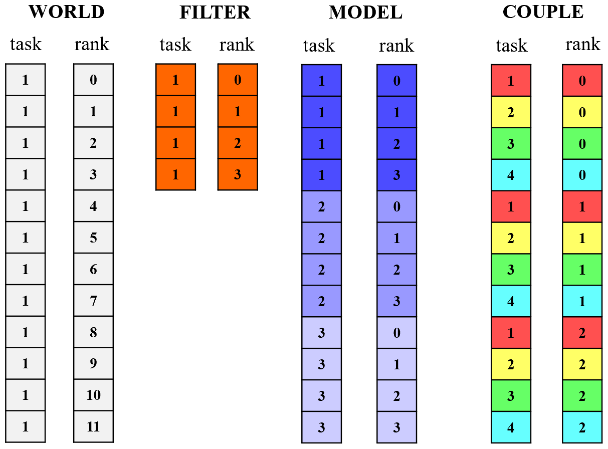
Figure 1Example configuration of MPI communicators for one model realization in the NAQPMS (a) and three model realizations in the NAQPMS-PDAF of the communicator MPI_COMM_MODEL (b), MPI_COMM_COUPLE (c), and MPI_COMM_FILTER (d). The four colors represent the decomposition of processors for different aims. The area outlined by dashed black lines is the NAQPMS-PDAF. The dimension of the state vectors is also shown (e).
The apportionment of the processes with three communicators is shown in Fig. 1b–d with four processes within one model realization and a total of three ensemble members in the NAQPMS-PDAF. The number of model communicators is equal to that of ensemble members, with four processors within one model communicator in Fig. 1b. This indicates that the three ensemble members are running simultaneously with different initial perturbations. Figure 2 shows the processor layout of four communicators with the same configuration in Fig. 1. The filter communicator performs the core DA algorithm with four processors, the number of which is equal to that of processors in one model realization. In the filter communicator, only the processes in one ensemble member (four orange processors in Fig. 2) are used, and other processes remain idle during the ensemble DA. The couple communicator with four tasks (three processors in one task) is used to exchange information between the processes in the model and filter communicator before and after the DA step. The number of processors in one couple communicator is equal to that of the ensemble members. This indicates that one task in the couple communicator focuses on the same subdomain for collecting the information in ensemble simulations and the filter algorithm. The different decompositions between the model communicator and filter communicator as well as the couple communicator (Fig. 1b–d) are explained below.
The main program flow of the NAQPMS-PDAF in this study can be generalized in the following steps:
- 1.
initialization of MPI (MPI_COMM_WORLD);
- 2*.
initialization of three communicators (MPI_COMM_MODEL, MPI_COMM_FILTER and MPI_COMM_COUPLE);
- 3.
initialization for the NAQPMS;
- 4*.
initialization of variables for the PDAF;
- 5.
time loop with ensemble simulations and filter:
- a*.
update the model variables corresponding to state vectors in the NAQPMS;
- b.
advance the NAQPMS to the next assimilation time step;
- c*.
update the state vector after ensemble integration;
- d*.
filter step;
- a*.
- 6*.
finalization of the PDAF and NAQPMS.
The program flow shown above is based on the original flow of the NAQPMS, while the steps denoted by asterisks are additionally added by the PDAF due to the online coupling. After the core modification of two-level parallelization discussed above, three communicators are initialized in steps 1 and 2 at the very beginning. The model initialization of the NAQPMS proceeds in step 3. Each processor in the communicator MPI_COMM_MODEL opens the same common input file, such as meteorological data model configuration files, and a different input file of initial perturbed emission for the ensemble initialization (see Sect. 2.3.3). One processor within one model realization (communicator MPI_COMM_MODEL) reads different parts of the opened data file corresponding to the different subdomains assigned in steps 1 and 2.
In step 4, the variables (size of state vectors, domain setting in the DA framework, and so on) in the PDAF are initialized. The dimension of the state vectors used in the DA framework is specially redesigned to meet the needs of domain decomposition and the observation operator in the PDAF. As shown in Fig. 1e, ix, iz, and iy are the number of grids in the longitudinal, latitudinal, and vertical directions, respectively. S represents the specific state variables, and the number of variables is N. Specifically, the dimensional order from outside to inside the state vector is ix, iz, and iy variables. As shown in Fig. 1c, the domain decomposition follows the longitudinal direction. This indicates that regardless of the position to be cut in the longitudinal direction, the slice has full three-dimensional information with all variables that can map onto the observation. The observation vectors have the same configuration, while they have only one variable. The time loop of model simulations and filter update in the NAQPMS-PDAF occurs in step 5. Step 5b represents the evolution of air pollutants under atmospheric physical and chemical processes, which follows the raw source code of the NAQPMS. The ensemble filter algorithm is implemented after advancing the NAQPMS at the end of each time loop of ensemble simulations. The number of time steps is set in the initialization of the NAQPMS, and the number of filter steps is set in that of the PDAF, while these two terms are not necessarily the same. Before and after the time loop of the NAQPMS, two modules, mainly including routines from_field and into_field, are run (step 5a and step 5c). The routine from_field collects all model state vectors from each processor on one model communicator (MPI_COMM_MODEL), which is updated by the filter period at the previous cycle. Afterward, the routine from_field apportions the state vectors into subvariables. The routine into_field does the reverse, similar to that in the routine from_field. After the performance of the routine into_field, each process gains the state vectors by cutting along the longitudinal direction. The domain decomposition in the model and couple communicator, as well as the filter communicator, is different, as discussed in step 4, which seems to be a waste of computational efficiency. However, the vector states used in this study (see Sect. 2.3.3) are only a rare part of all variables in the NAQPMS. Hence, it has little impact on the DA framework, and the parallel efficiency is high, which is discussed in Sect. 3.1. In step 5d, the ensemble filter is called to update the state vectors with observations, which are implemented in the source code of the PDAF, which may not need to change unless a new filter algorithm is added. In step 6, the variables used in the NAQPMS and PDAF are deallocated, and timing information and memory information are provided that can check the program run and help to optimize the program.
In practice, we developed a pre-/postprocessing auxiliary program written in Python 3.6 for the task of constructing a three-dimensional data structure of observation and plotting figures for different aims. We also set a variable to identify each run in the NAQPMS-PDAF and to create new files corresponding to that variable to save the data to avoid frequently removing and overwriting the data that we need.
2.3.2 Ensemble DA algorithm
The error-subspace transform Kalman filter (ESTKF, Nerger et al., 2012) used in this study is a recently developed EnKF variant. Firstly, EnKF originated from the fusion of Kalman filter theory and Monte Carlo estimation method. By providing flow-dependent estimates of first-guess forecast error, the EnKF can potentially provide analysis and forecasts that are much more accurate than DA schemes which assume that the background error does not vary in time (Whitaker and Hamill, 2002). Secondly, EnKF and its variants can be categorized as deterministic filters (ETKF (the ensemble transform Kalman filter), ESTKF, and so on) and as stochastic filters which assimilate perturbed observations (original EnKF). On the one hand, the deterministic filter can only use small ensemble sizes for high-dimensional problems, while stochastic filters need large ensemble sizes (Lawson and Hansen, 2004). On the other hand, the stochastic filters may add another source of sampling error and underestimate the analysis update because observations assimilated are perturbed. Thirdly, ESTKF is derived from the singular evolutive interpolated Kalman filter (SEIK, Pham et al., 1998) by combining the advantages of the SEIK and ETKF. These three filters are essentially equivalent apart from computing the ensemble transformation in the error subspace (Vetra-Carvalho et al., 2018). The ESTKF can exhibit better properties than the SEIK filter, like a minimum ensemble transformation such as the ETKF. Nerger et al. (2012) conducted a series of numerical experiments to compare the performance of SEIK, ETKF, and ESTKF using deterministic and random ensemble transformations. They found that the performance for the ESTKF and ETKF is better than that for the SEIK filter, with ESTKF having a slightly lower computational cost. The ESTKF is outlined in this section.
As an EnKF-based deterministic filter, the algorithm can be decomposed into the steps of forecasting and analysis. The forecast step of any EnKF implementation is the same, and more details can be found in Houtekamer and Zhang (2016). The forecast propagates the states and the corresponding error covariance matrix forward in time from a previous analysis at to the next observation time t=tk. The numerical model Mk, the NAQPMS in this study, is used to propagate ensemble members during certain time steps:
where is the model forecast realization at t=tk and is the model analysis realization at . Ne is the number of ensemble members and . The size of state vector () is Nx. The state vector in the forecast phase can be estimated and is approximated by the ensemble mean:
In the analysis step at t=tk, the filter algorithm transforms a matrix of forecast ensemble into a matrix of analysis ensemble , and the time index k is omitted because the time of all the implementations during the analysis step is constant.
where Xa and Xf denote an ensemble matrix in which each of the Ne columns represents one model realization of the analysis and forecast, respectively (. Ne is the number of ensemble members and . is the analysis/forecast realization of ensemble member i. is a identify matrix of size Ne×1. Furthermore, ω transforms the ensemble mean with size Ne and transforms the ensemble perturbations with size Ne×Ne. The sample error covariance matrix approximated with an ensemble is only a low-rank approximation of the true state, and its rank is at most Ne−1 (Gillet-Chaulet, 2020). This property is utilized in the ESTKF to compute the ensemble matrix transformed in this subspace (Nerger et al., 2020). The error-subspace matrix is computed by
where it is a projection matrix of size given by the set of equations as follows:
The state vectors are mapped into the observation space with the observation operator H in the analysis step by
where ε is the observation error assumed to be an unbiased Gaussian distribution and it has known observation error covariance matrix R. In the error subspace of the ensemble DA, an ensemble transform matrix is computed especially with Eq. (5) as
where the factor ρ with is defined as the forgetting factor. The forecast error covariance matrix is inflated by the forgetting factor ρ to overcome the undersampling issues (Anderson and Anderson, 1999; Pham et al., 1998).
Thus, the weight vector ω and matrix are given by
where is the symmetric square root computed from the eigenvalue decomposition. Apart from the inflation discussed above, localization technology is also utilized for filter stabilization. Only observations within a certain horizontal localization radius are used when updating a local analysis. In addition, each observation is weighted with distance, which is performed by adjusting Eqs. (7) and (8). A fifth-order polynomial function with compact support (Gaspari and Cohn, 1999) is used to compute the weight of the horizontal localization. We set the horizontal localization radius and forgetting factor to 200 km and 0.96 according to a series of sensitivity tests in the Supplement and other related studies (Kong et al., 2021; Zhao et al., 2020; Y. Cheng et al., 2019; Ma et al., 2020). Three adjacent grids are considered with the influence of observations of the vertical localization, which is a simple setting.
2.3.3 Model configuration
To reduce the uncertainty of meteorological data, three nested model domains for the WRF are performed with horizontal resolutions of 45, 15, and 5 km, as shown in Fig. 3a. The vertical coordinate system consists of 40 terrain-following levels with 27 layers within 2 km, which is especially designed for research on assimilating measurements, including vertical information. The third domain of the WRF is used as the only model domain in ensemble simulations in the NAQPMS-PDAF for saving computing resources and avoiding the error from performing multi-DA for different domains. The WRF is driven by the NCEP FNL data. The lateral and upper boundary conditions were taken from the global chemistry-transport Model for OZone and Related chemical Tracers (MOZART) v2.4 with a 2.8∘ horizontal spatial resolution (Brasseur et al., 1998; Hauglustaine et al., 1998). Anthropogenic emissions were provided by the 0.25∘ Multi-resolution Emissions Inventory for China (MEIC, http://www.meicmodel.org, last access: 14 September 2021).
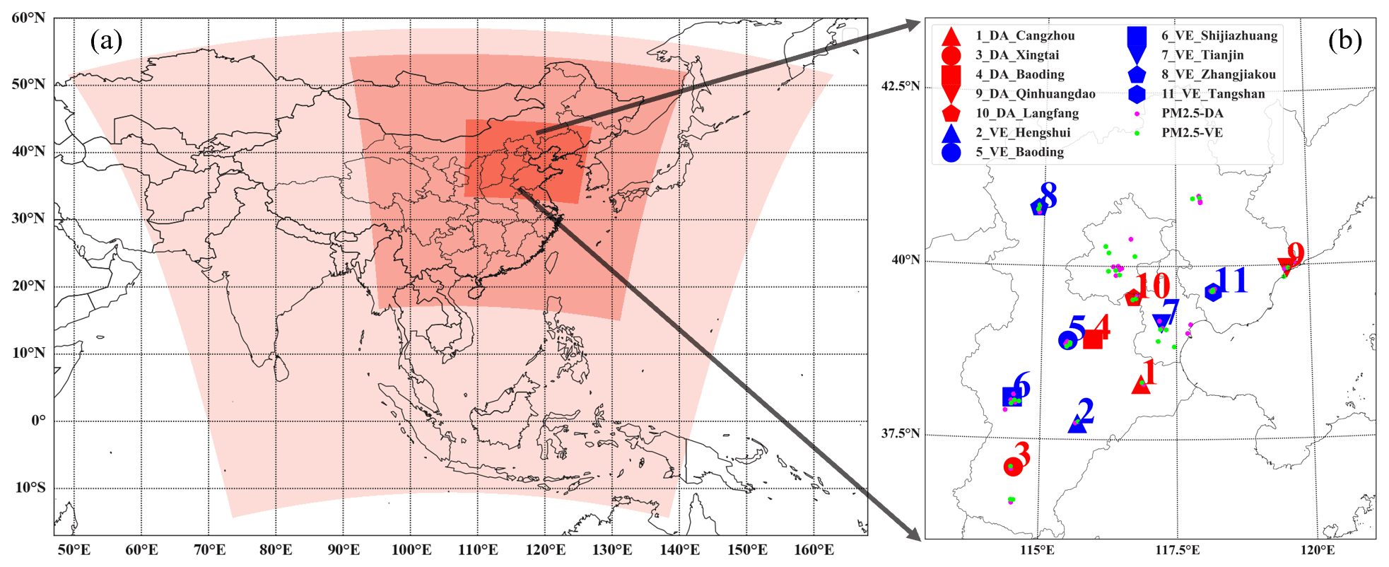
Figure 3The model domain in the WRF simulation (a) and the location of observation stations (b). Three red regions with different transparencies identify three mode domains (a). Red dots denote ground-based lidar sites that are assimilated, while blue dots denote verified sites (b). Similarly, pink dots denote assimilated surface PM2.5 sites, while green dots denote verified sites. The serial number denotes ground-based lidar sites.
The state vectors include the mass concentration of ammonium, sulfate, nitrate, black carbon (BC), organic carbon (OC), soil particulate matter in PM2.5, soil particulate matter in PM10, sea salt, fine dust, coarse dust, and RH (relative humidity). RH, one of the state vectors, is used to map the model space into the observation space. The state vectors are all from the IMPROVE equation. The ensemble of initial chemical conditions is generated by perturbing the emissions based on their error probability distribution functions (PDFs). The PDFs are assumed to be Gaussian distributions, and the uncertainty of each species follows the evaluation in Streets et al. (2003) and Zhang et al. (2009) (12 % for SO2, 31 % for NOx, 68 % for volatile organic compounds (VOCSs), 53 % for NH3, 70 % for CO, 132 % for PM10, 130 % for PM2.5, 208 % for BC, and 258 % for OC). In practice, a set of perturbation factors is implemented with the Schur product to the original emissions. An isotropic correlation model is utilized to impose a horizontal correlation of disturbed emissions. Following Kong et al. (2021), the decorrelation length is specified as 150 km in this study. A total of 20 smooth pseudorandom perturbation fields of perturbation factors are generated for each species. The observation error of the surface PM2.5 measurement is set as 8 µg m−3 to account for measurement and representativeness (Ma et al., 2019). However, the observation error of ground-based lidar measurements is set as 10 % of the mean aerosol extinctions in reference to other studies on lidar DA (Sekiyama et al., 2010; Y. Cheng et al., 2019; Ma et al., 2020) due to a lack of specialized study of the error of lidar measurements.
2.4 Observational data
The extinction coefficients used in this study are ground-based lidar measurements from 11 sites. As shown in Fig. 3b, 11 lidar sites (red and blue dots) are distributed within the NCP with serial numbers from 1 to 11. The ground-based lidar from no. 1 to no. 6 with AGHJ-I-LIDAR (HPL: high-energy scanning pulse lidar) (Fan et al., 2019; Shi et al., 2020; D. Wang et al., 2020) is distributed south of the NCP, while the lidar from no. 7 to no. 11 with LGJ-01 (Sun et al., 2019) is located north of the NCP. These two lidar systems have similar specifications, with an energy of approximately 25 mJ and a pulse repetition rate of 20 Hz. The tunable time resolution is from 1 to 5 min, and the vertical resolution is 15 m. The blind ozone height is 300 m for both lidar types. Hourly extinction coefficients profiles at 532 nm which can represent vertical distribution of aerosols are averaged from the raw lidar measurements to improve the signal-to-noise ratio and meet the time resolution of the numerical model. To meet the model domain, 40 layers are generated from the raw lidar data by a piecewise cubic interpolating Bézier polynomial (Alfeld, 1984) using SciPy (Virtanen et al., 2020). As shown in Fig. 3b, mass concentration observations of surface PM2.5 (green and pink dots) on the NCP are obtained from the China National Environmental Monitoring Centre (CNEMC) (http://www.cnemc.cn/, last access: 20 May 2021).
The Cloud-Aerosol Lidar and Infrared Pathfinder Satellite Observation (CALIPSO) mission (http://www-calipso.larc.nasa.gov/, last access: 20 May 2021) is the first satellite-borne lidar specifically designed for aerosol and cloud study and is a collaborative effort between the NASA Langley Research Center (LaRC), Centre National d'Etudes Spatiales (CNES), Hampton University (HU), Institut Pierre-Simon Laplace (IPSL), and Ball Aerospace and Technologies Corporation (BATC) (Winker et al., 2009). CALIOP is an elastic backscatter lidar that is aboard CALIPSO. Vertical profiles of aerosol and cloud backscatter coefficients at 532 and 1064 nm, as well as depolarization ratio profiles at 532 nm from −0.5 to 30 km, are available from CALIOP. CALIOP has a horizontal spatial resolution of 5 km and a vertical spatial resolution of 40 m. The extinction coefficients at 532 nm from the CALIOP level 2 version 4.20 are used in this study for independent validation of the DA experiments. A total of 52 CALIOP orbits are included within the model domain for April 2019.
The Aerosol Robotic Network (AERONET, https://aeronet.gsfc.nasa.gov/, last access: 9 September 2021) is a global network of autonomously Cimel Sun photometer measurements that can provide high-quality key aerosol optical parameters at eight spectral bands within a range from 340 to 1020 nm (Holben et al., 1998). AOD data from the AERONET version 3 level 2.0 database, which has assured quality after the screening of clouds, are used as the independent measurement to evaluate the DA performance. AOD data at 532 nm, used as independent validation dataset, are calculated from the AERONET AODs at 440, 500, and 670 nm by quadratic polynomial interpolation (Eck et al., 1999; H. Wang et al., 2020).
2.5 Experimental setting and evaluation method
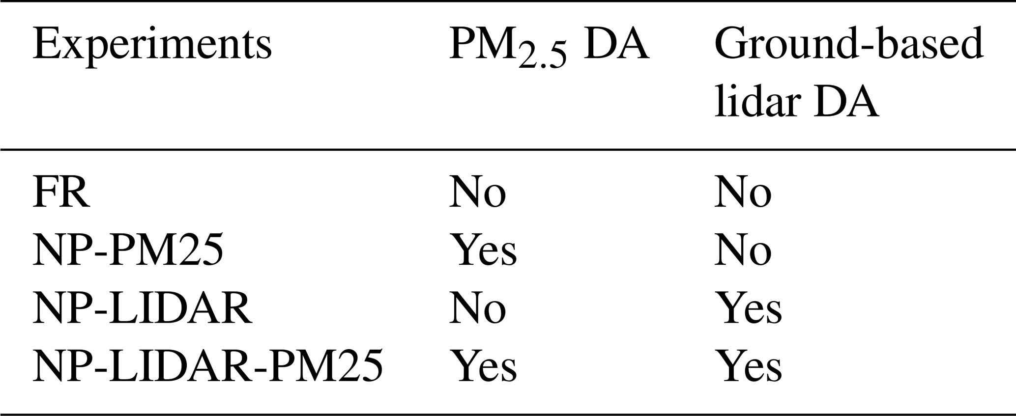
To investigate the performance of the NAQPMS-PDAF with real observations and the impact of assimilating vertical observations into the CTM, a total of four experiments with a 30 d study period running from 00:00 UTC on 1 April 2019 to 18:00 UTC on 30 April 2019 were conducted. As we care more about the variables related to extinction coefficients and surface PM2.5, which exclude most gaseous pollutants, the number of state variables used and output in the assimilation part of the NAQPMS-PDAF was smaller than those in the NAQPMS. We ran the NAQPMS for 3 d from 00:00 UTC on 29 March 2019 to 23:00 UTC on 31 March 2019 as a spin-up for NAQPMS-PDAF. As summarized in Table 1, the first experiment of the NAQPMS-PDAF was free running (FR) without assimilating any observations, providing a comparison with the following DA experiments. An experiment assimilating the surface PM2.5 (NP-PM25) was performed to investigate the performance of the NAQPMS-PDAF. An experiment assimilating only the extinction coefficients measured by ground-based lidar (NP-LIDAR) was designed to examine the impacts of assimilating vertical observations of aerosols. An experiment simultaneously assimilating lidar measurements and surface PM2.5 simultaneously (NP-LIDAR-PM25) was conducted to probe the combined impacts of the fusion of multiple observations containing surface and vertical observations.
The EnKF system used in our work provides possibilities for using a short assimilation window to have the ensemble perturbations evolve linearly (Houtekamer and Zhang, 2016; Y. Liu et al., 2019), while a 4D-Var system needs to keep a long window to reduce the effect of the initially specified covariances (Pires et al., 1996). Therefore, we choose 1 h as assimilation window in NAQPMS-PDAF as other similar studies (Y. Liu et al., 2019; Ma et al., 2019; Ha et al., 2020) do. The assimilation cycle is set as 1 h. On the one hand, our work focuses on investigating the parallel performance of NAQPMS-PDAF and the improvement of vertical profile simulations after assimilating aerosol extinction coefficient profiles. The performance of ensemble forecast after ensemble filter is not the focus. On the other hand, the 6 h assimilation cycle used in similar studies (Liu et al., 2011; Ma et al., 2019, 2020; Pang et al., 2018) follows the model configuration of assimilating satellite data with coarse temporal resolution. However, the lidar measurements used in our work can provide large temporal variability with temporal resolution of 1 h. In order to investigate the difference of different assimilation cycle on the analysis and forecast, an extra experiment assimilating lidar measurements at a cycle of 6 h (NP-LIDAR-6HR) has been performed in the Supplement (Table S1). The RMSE value of the NP-LIDAR and NP-LIDAR-6HR experiment is 0.16 and 0.18 km−1, respectively (Fig. S1). The Pearson correlation coefficient (CORR) values of these two experiments are 0.91 and 0.89 (Fig. S1). The performance of the mean bias (BIAS) of the NP-LIDAR experiment is slightly better than that of the NP-LIDAR-6HR experiment with 93 % and 92 % scatters within | BIAS | <0.25. Other detailed discussion can be found in the Supplement. It can be found that the statistic performance at cycle of 1 h is better than that at a cycle of 6 h, which supports the setting of cycle of 1 h in our work.
During the evaluation, four basic statistical metrics, the root mean square error (RMSE), the mean absolute error (MAE), BIAS, and CORR, were calculated against the measurements. RMSE and MAE are widely used in model evaluations to assess the absolute deviation between the model output and observations, and the combination of these metrics is often required to assess model performance (Chai and Draxler, 2014). BIAS is an indicator to intuitively show the degree of datasets prone to overestimation or underestimation. The CORR can be used to represent the extent to which a dataset satisfies a linear relationship (Su et al., 2018).
3.1 Scaling behavior
To assess the computational efficiency of the NAQPMS-PDAF described in Sect. 2.3 in high-performance computing (HPC), we performed a scaling study on the HPC subsystem of the Big Data Cloud Service Infrastructure Platform (BDCSIP) located in Beijing (China). The HPC subsystem of the BDCSIP (HPC-BDCSIP) consists of 313 Intel Xeon scalable gold computation nodes, and it entirely has 12 520 processors and nearly 88 TB main memory. The cores within one computation node is 40, 157 of which have 384 GB main memory and the others have 192 GB main memory, and runs at 2.50 GHz. All computing nodes are connected by a 100 Gbps EDR (enhanced data rate) InfiniBand network. The data storage subsystem of the BDCSIP can be accessed by all computing nodes through InfiniBand, and the total capacities are more than 25 PB. The HPC-BDCSIP achieves a performance of a linear system package with 1.0 Pflops.
The scaling of the NAQPMS-PDAF can be investigated through strong and weak scaling tests. A strong scaling is the parallel performance with the overall workload remaining fixed but with the number of processors increasing, while the weak scaling is when the workload assigned to each process remains constant with an increase in processors (Sharples et al., 2018). The runtime is expected to decrease with an increasing number of processors in strong scaling, while the runtime is expected to be constant in weak scaling. As the strong scaling properties of the NAQPMS and PDAF have been examined in previous studies (H. Wang et al., 2017; Nerger and Hiller, 2013), the NAQPMS-PDAF, an online coupled system of the NAQPMS and PDAF, is needed to first perform both strong and weak scaling tests to investigate the computational efficiency. To balance computational resources and representativeness, we performed 24 analysis steps (from 18:00 UTC on 8 April 2019 to 17:00 UTC on 9 April 2019) for the scaling studies. For each compute node, 25 cores were used, which was found to be the best configuration under preliminary tests considering both execution time and memory requirements. Since the decomposition of the model domain in the MPI is along the longitudinal grids, as discussed in Sect. 2.3.1, the number of processors of one realization must be set as the value, which can be divided evenly between the number of longitude grids (300 in this study) and the division between the total number of processors and the number of ensemble members. Therefore, in the strong scaling study, we set the ensemble size as a constant, 20, and increased the processors from 100 to 2000 with a total of 10 tests, which are shown in Table 2. The amount of ensembles was raised from 2 to 50 with a sum of eight tests in the study of weak scaling. Parallel efficiency (E) (Sharples et al., 2018) can be used to investigate the scalability of the NAQPMS-PDAF:
where Ess(bq) is the parallel efficiency representing strong scaling and Ews(bq) is the parallel efficiency representing weak scaling. b is the number of processors used in the base test and T(b) is the execution time with b processors. bq is the number of processors used in different tests with bq=np. As shown in Table 2, b is set as 100 in the strong and weak scaling.
Table 2Number of realizations, compute nodes, and processors utilized for the study of strong and weak parallel efficiency for the NAQPMS-PDAF. The number of cores within one compute node is set as 25.
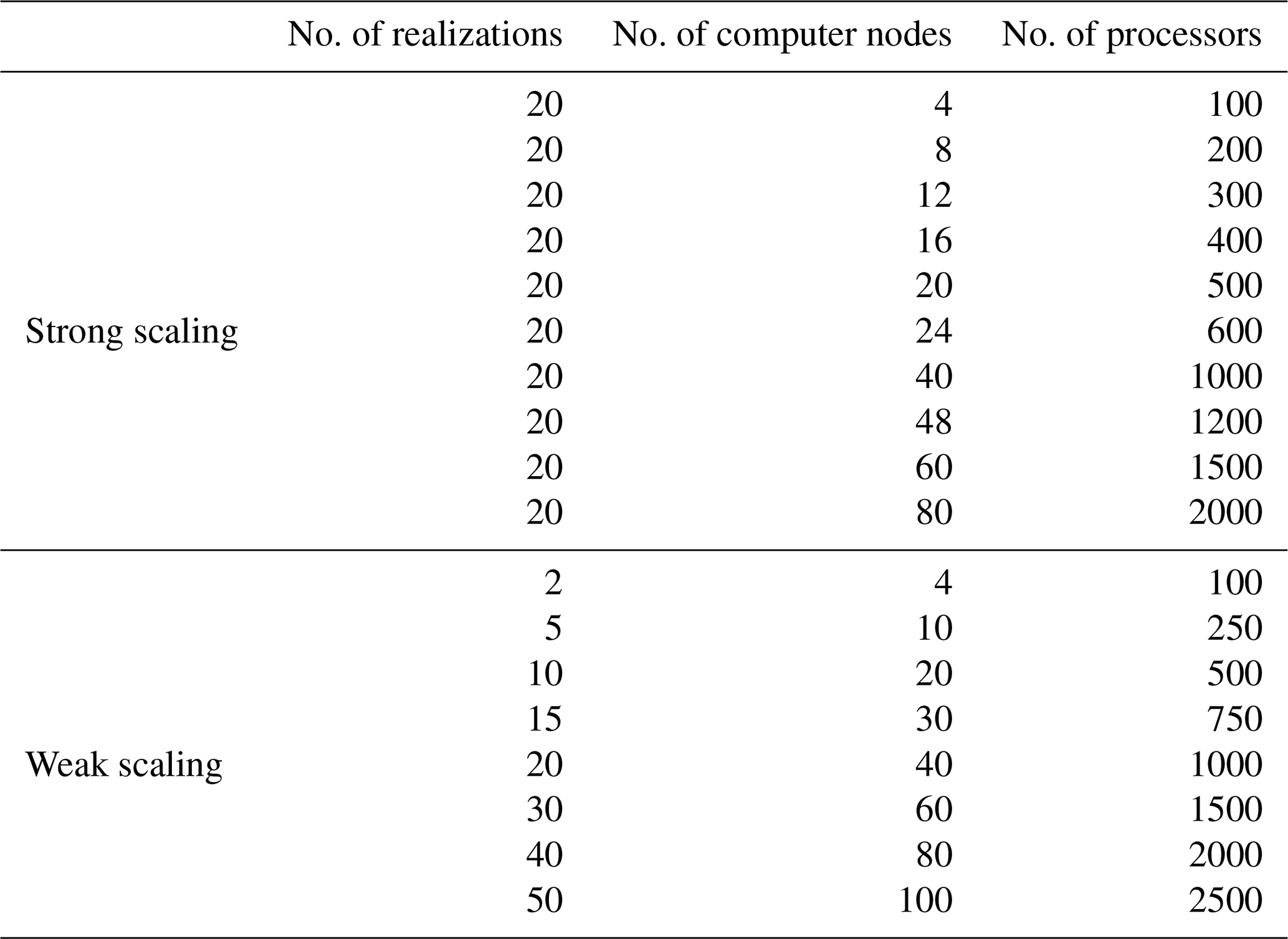
Figure 4 shows the execution times per model hour (blue) and strong scaling efficiency (orange) for different processors. The abscissa is the number of processers and corresponding ensemble size, which is set as 20 in the strong scaling test. The entire blue line decreased as an exponential function and a nearly 12-fold decrease in time with a 20-fold increase with processors. When the number of processors was from 100 to 600, the execution time decreased rapidly, and strong scaling efficiency remained very high (>0.85). During this period, the speed increased with more processors apportioned to one model realization. When the number of processes was increasing from 1000 to 2000, the execution time showed a slight decrease, and strong scaling efficiency decreased rapidly from ∼0.77 to 0.6. During this period, the number of processors for one model realization was further increasing, leading to too much consumption of data transfer in the NAQPMS-PDAF. As a result, the same increase in processors had less improvement in the strong scaling efficiency than that in the former period. Referring to the results in the strong scaling behavior, 50 processors were used for each model realization in this study. However, the results of the strong scaling behavior shown here were related to the configuration of the NAQPMS-PDAF and the capability of HPC.
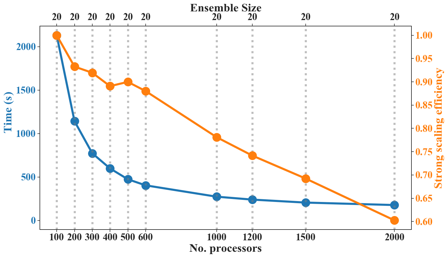
Figure 4Timing information (blue line) and scaling behavior (orange line) for the NAQPMS-PDAF for a strong scaling test. The ensemble size is a constant of 20 and increases the processors from 100 to 2000 with a total of 10 tests.
Figures 5 and 6 show timing information and weak scaling efficiency for the weak scaling test. The abscissa is the ensemble size and corresponds to the number of processors. The ratio of the number of processors and ensemble members is a constant, 50, which was acquired on the strong scaling test. The execution time per model hour was averaged during the 24 h runs described before, which was the same as the strong scaling test. The orange line shows the execution time of model integration, which dominated the overall time. With the ensemble size increasing from 2 to 50, the execution time of initialization (blue line) and finalization (red line) of the NAQPMS-PDAF increased from 4.6 to 36.8 s and 4.8 to 37.9 s, respectively. The execution time of ensemble simulations (orange line) dominated the overall time and increased from 223 to 277 s. The execution time of assimilation remained steady and increased from 1.3 to 1.6 s.
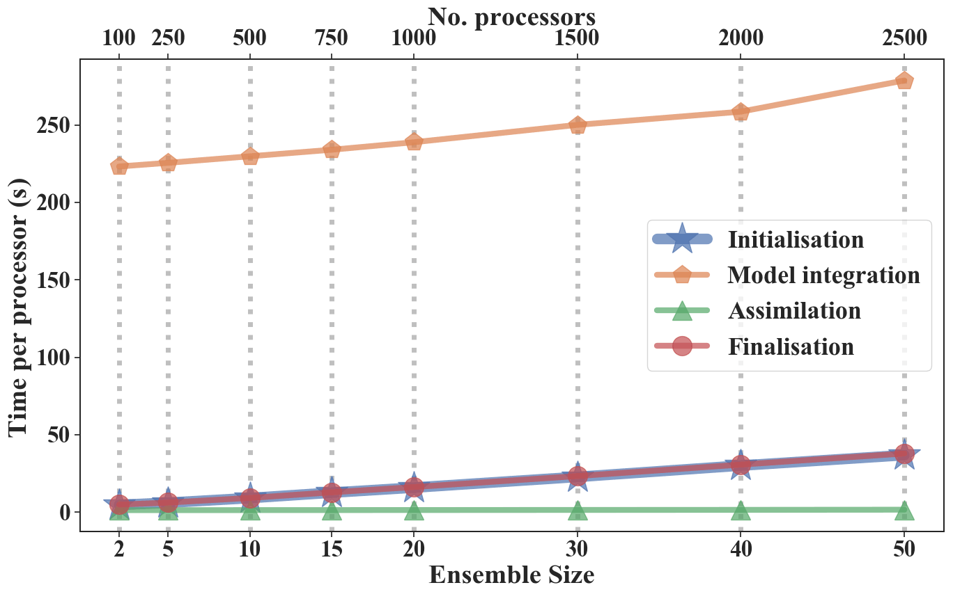
Figure 5Timing information for the NAQPMS-PDAF for a weak scaling test. The blue line shows the execution time for initialization. The orange line shows the execution time for model integration. The green line shows the execution time for assimilation. The red line shows the execution time for finalization. A total of 50 processors are apportioned to each ensemble member.
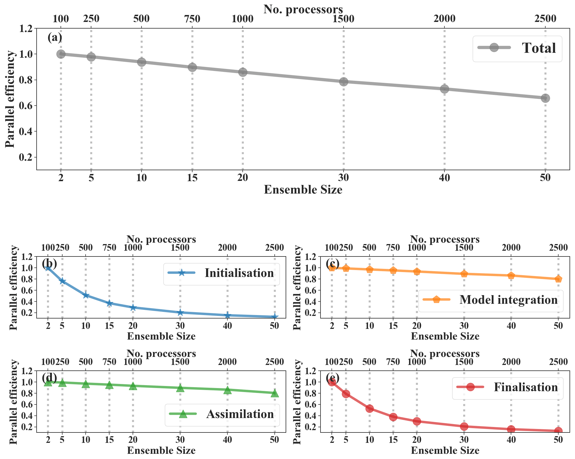
Figure 6Weak scaling behavior for the NAQPMS-PDAF. The gray line shows the parallel efficiency for all processes. The blue line shows the parallel efficiency for initialization. The orange line shows the parallel efficiency for model integration. The green line shows the parallel efficiency for assimilation. The red line shows the parallel efficiency for finalization. A total of 50 processors are apportioned to each ensemble member.
As shown in Fig. 6, the weak scaling efficiency of model integration decreased from 1.0 to 0.8 as the ensemble size increased from 2 to 50. Although the weak scaling efficiency of initialization and finalization decreased rapidly from 1.0 to 0.12, showing slightly poor parallel behavior, the execution time of these two parts only accounted for a small portion of the overall time. The weak scaling behavior of the assimilation step in the NAQPMS-PDAF was the best and decreased from 1.0 to 0.81. In summary, the total weak scaling efficiency decreased from 1.0 to 0.7, which showed comparable results compared with other coupled systems with the PDAF, such as the TerrSysMP-PDAF (Kurtz et al., 2016). As a result, the coupling between the NAQPMS and PDAF worked very well in a technical sense. In the above scaling study, real ensembles were used, and the results may have been affected by load imbalance to some extent due to heterogeneous ensembles. We set the task exclusively when using HPC to avoid the load affected by other users.
3.2 Evaluation of the data assimilation framework
3.2.1 Ensemble performance
The results of DA analysis and subsequent 1 h simulation depend on the ensemble performance to a large extent. The comparison of the prior RMSE and the prior total spread is utilized to measure the ensemble spread in this study. The prior RMSE is defined as , where is an assimilated observation, is the prior ensemble mean of the observation mapped from the background simulation and p is the number of assimilated observations. The prior total spread is defined as , where is the observation error variance and is the prior ensemble variance in the observation space. The prior RMSE and the prior total spread should be balanced in a well-calibrated system (Houtekamer et al., 2005).
Figure 7 shows the prior RMSE and the prior total spread of extinction coefficients at 50, 150, 502, and 1000 m and surface PM2.5. As we can see in Fig. 7a, these two factors show comparable magnitudes and trends in the surface PM2.5 and extinction coefficients at 50 m, indicating that the NAQPMS-PDAF is well balanced. However, the total spreads of extinction coefficients at altitudes of 150, 502, and 1000 m show an insufficient spread. The same scenario occurred on the surface PM2.5 in Peng et al. (2017), in which they found that it was affected by heavy pollution with much larger RMSEs of PM2.5. The insufficient spread of extinction coefficients at higher altitudes was probably because the initial ensemble was disturbed mostly near the surface, and high altitudes only have a small number of elevated sources. Air pollution at high altitudes is mostly due to transport and secondary formation and seldom has direct sources.
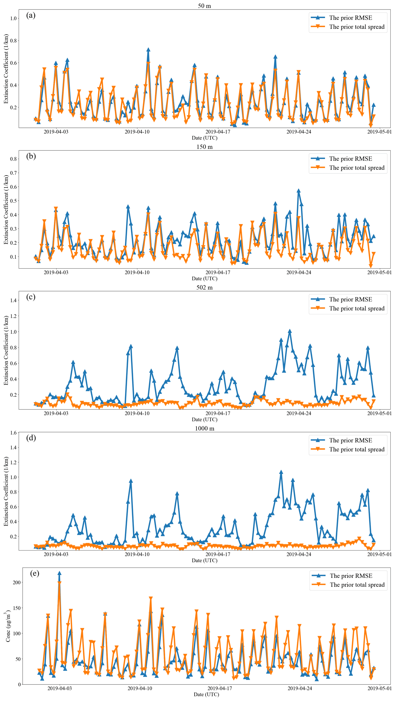
Figure 7Time series of prior RMSE and total spread over all observations for (a) extinction coefficients at 50 m, (b) extinction coefficients at 150 m, (c) extinction coefficients at 502 m, (d) extinction coefficients at 1000 m, and (e) the surface PM2.5.
3.2.2 Internal check
In this section, an internal check (or called sanity check), a comparison of analyses and subsequent 1 h simulations (or called forecasts) of DA experiments with assimilated observations are performed to characterize the performance of the NAQPMS-PDAF. The extinction coefficients measured by ground-based lidars and simulated by the NAQPMS-PDAF from the height of the blind zone (300 m) and the height of 4275 m are chosen as sample data.
Figure 8 shows the extinction coefficient scatters from the model versus the ground-based lidar measurements averaged over five assimilated sites (DA sites) and six verified sites (VE sites) for the four numerical experiments. Figure 9 shows the frequency distribution of the forecasts and the analysis of the corresponding experiments shown in Fig. 8. As shown in Fig. 8a and i, a variety of scatters are distributed outside the 2:1 line, showing that aerosol extinction coefficients were obviously underestimated in the FR experiment, especially below 1200 m. This indicates that the numerical model has deficiencies in reproducing pollutant plumes, especially inside the boundary layer, compared with lidar measurements. The underestimation of the aerosol vertical distribution, which commonly exists in other CTMs such as POLYPHEMUS and WRF-Chem (Wang et al., 2013; Ma et al., 2020), is attributed to numerous uncertainties in direct sources (e.g., emissions and initial/boundary conditions), physical and chemical processes concerning the formation of aerosols (e.g., nucleation, condensation, horizontal advection, and vertical diffusion), and model parameterizations, as well as uncertainties in the meteorological field.
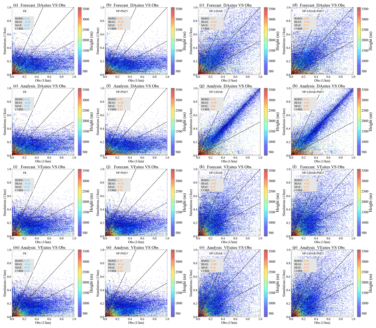
Figure 8Scatterplots of the modeled hourly extinction coefficients at 550 nm versus the ground lidar hourly aerosol extinction coefficients at 532 nm (km−1) of forecasts of FR (a)/(i), forecasts of NP-PM25 (b)/(j), forecasts of NP-LIDAR (c)/(k), forecasts of NP-LIDAR-PM25 (d)/(l), analysis of FR (e)/(m), analysis of NP-PM25 (f)/(n), analysis of NP-LIDAR (g)/(o), and analysis of NP-LIDAR-PM25 (h)/(p), which are averaged among DA sites/VE sites. The three dashed black lines correspond to the 1:2, 1:1, and 2:1 lines in each panel.
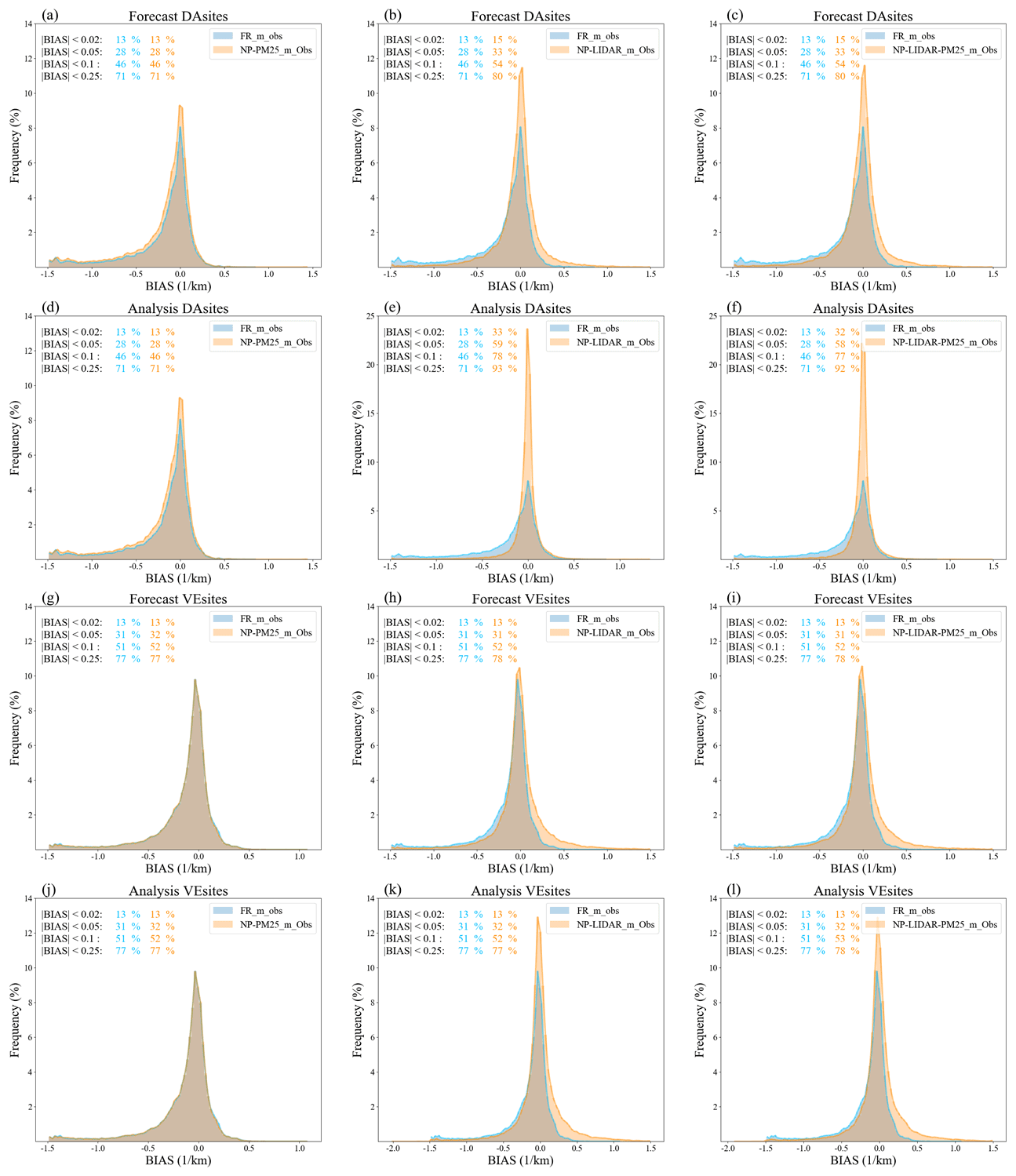
Figure 9Frequency distributions of BIAS of forecasts of NP-PM25 versus FR (a)/(g), forecasts of NP-LIDAR versus FR (b)/(h), forecasts of NP-LIDAR-PM25 versus FR (c)/(i), analysis of NP-PM25 versus FR (d)/(j), analysis of NP-LIDAR versus FR (e)/(k), and analysis of NP-LIDAR-PM25 versus FR (f)/(l), which are averaged among DA sites/VE sites.
As shown in Fig. 8c and g, most scatters showing underestimation in the FR experiment are distributed between the 1:2 line and 2:1 line in the NP-LIDAR experiment. In the NP-LIDAR experiment (Fig. 8c, g), the absolute value of the negative BIAS value decreases from 0.20 km−1 (FR) to 0.02 (0.04) km−1, and the CORR rises from 0.33 (FR) to 0.91 (0.72) in the analysis (forecast). The RMSE value decreases from 0.42 km−1 (FR) to 0.16 (0.27) km−1, and the MAE value decreases from 0.25 km−1 (FR) to 0.08 (0.16) km−1 in the analysis (forecast) in the NP-LIDAR experiment. The frequency distribution of extinction coefficients is more squeezed around the value of 0.0 km−1 with higher peaks in the NP-LIDAR experiment than in the FR experiment (Fig. 9b, e). In the analysis, 46 % (13 %) of the extinction coefficient BIASs are within ±0.1 km−1 (±0.02 km−1) in the FR experiment, while 78 % (33 %) of the BIAS is achieved within ±0.1 km−1 (±0.02 km−1) in the NP-LIDAR experiment, respectively. The 1 h forecast also shows a positive performance with a relatively poor statistical performance compared with that in the NP-LIDAR experiment due to the attenuation of the impact of DA during the model simulation. This suggests that after assimilating the vertical profiles of extinction coefficients measured by ground-based lidars including vertical profile information, the underestimation is noticeably reduced. Moreover, the performance of NP-LIDAR-PM25 is generally comparable to that of the NP-LIDAR experiment, while the performance of NP-PM25 is also similar to that of the FR experiment. This indicates that assimilating surface PM2.5 measurements has a limited impact on higher layers in the analysis and 1 h forecast.
Maps of statistical metrics (RMSEs and correlation coefficients) between the modeled and surface-measured PM2.5 are presented to investigate the DA performance of the four experiments, which is shown in Figs. 10 and 11. The increments of specific metric indicate the difference of this metric between a DA experiment and the FR experiment. The increments in RMSEs (CORRs) of all sites are negative (positive) in the NP-PM25 experiment, with a range of approximately −60 % to −30 % (30 % to 80 %), and generally, the absolute value of those increments over the southern part of the NCP is larger than those over the northern part of the NCP (Figs. 10d and 11d). It shows pronounced improvement of directly assimilating surface PM2.5 measurements. The increments in RMSEs of most sites are negative in the NP-LIDAR experiment, with a range of approximately −40 % to −5 %, while a few sites have positive increments (Fig. 10e). However, the increments in CORRs of all sites are positive in the NP-LIDAR experiment at more than 20 % (Fig. 11e). These results indicate that only assimilating ground-based lidar measurements can improve the surface PM2.5 simulations of most areas by modifying the initial conditions of aerosol vertical profiles, especially under the view of linear trends, but there are still some deficiencies at some sites. The performance of statistical metrics on the surface (RMSEs and CORRs) in the analysis in the NP-LIDAR-PM25 experiment is similar to those in the NP-PM25 experiment because the last observation assimilated in NP-LIDAR-PM25 is the surface PM2.5 measurement and the first kind of observation (ground-based lidar measurements) has no direct impact (due to lidar blind zone) on the surface. However, the difference between the NP-PM25 and NP-LIDAR-PM25 experiments occurs in the forecast, which indicates that assimilating lidar measurements has a certain impact on the surface within 1 model hour and slightly degrades the performance of surface PM2.5 simulations (Fig. 10k). It can be concluded that the performance of the NAQPMS-PDAF in simulating surface PM2.5 is better than that in the FR experiment after assimilating surface PM2.5 measurements, ground-based lidar measurements, and both of these measurements. However, the performance of only assimilating surface PM2.5 measurements on the surface aerosol simulations is better than that of only assimilating ground-based lidar measurements. This could be explained by the relatively sparser distribution of lidar sites compared with surface PM2.5 measurement sites and the uncertainty in the spatial representation of lidar data (Liang et al., 2020), as well as the errors in the lumped variables of extinction coefficients with multiple contributions by different aerosol components. Moreover, the problem can also be attributed to the discordant relationship between aerosol mass concentration and extinction coefficients both in the simulation and measurements, which was noticed by Ma et al. (2020), and a simple bias correction method was proposed to fix this problem. The problem discussed above will be discussed in more detail in a separate study.
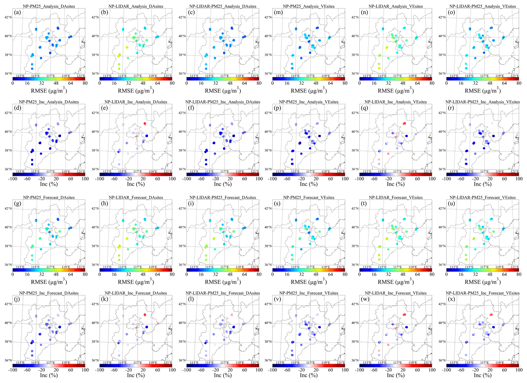
Figure 10Spatial distributions of the RMSEs (km−1) of the surface PM2.5 analysis (a, b, c), the increments in the RMSEs of the surface PM2.5 analysis (d, e, f), the RMSEs of the surface PM2.5 forecast (g, h, i), and the increments in the RMSEs of the surface PM2.5 forecast (j, k, i) for the NP-PM25, NP-LIDAR, and NP-LIDAR-PM25 experiments among DA sites. Panels (m)–(x) are the same as panels (a)–(l) but for VE sites.
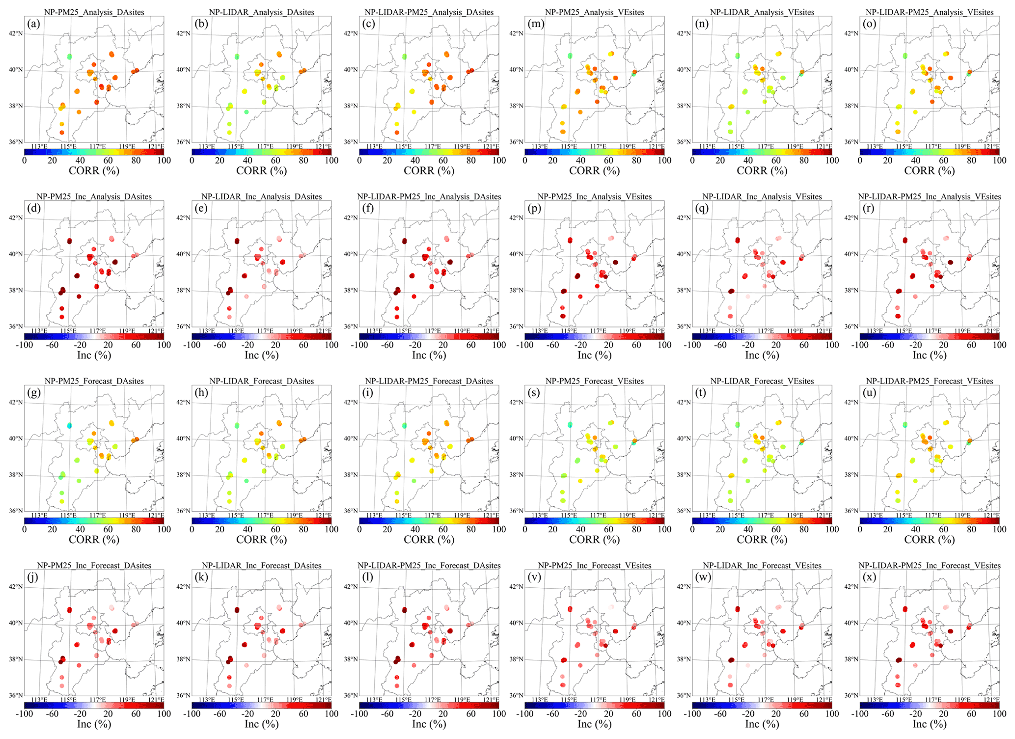
Figure 11Same as Fig. 10 but with CORR.
3.2.3 Independent validation
In this section, the DA performance of the NAQPMS-PDAF on the sites of the surface PM2.5 observations and ground-based lidar measurements that are not assimilated is investigated as the independent validation, as well as the independent CALIOP and AERONET measurements.
The extinction coefficients averaged over the six VE sites are underestimated with a BIAS of −0.14 km−1, showing a slightly better simulation performance compared with those at the five DA sites (Fig. 8i). In the NP-LIDAR experiment, the analysis and subsequent 1 h simulation performance of the four statistical metrics (RMSE of 0.30 and 0.30 km−1, MAE of 0.18 and 0.18 km−1, BIAS of 0.00 and −0.01 km−1, and CORR of 0.55 and 0.53) at VE sites is particularly similar (Fig. 8k, o), which shows a significant improvement compared with those in the FR experiment (Fig. 8i). This suggests that the initial chemical conditions at VE sites after the implementation of the ensemble filter of the previous step in the analysis show good consistency with the lidar observations which are not assimilated. The difference between the analysis and forecast at VE sites can be identified in Fig. 9h and k, where extinction coefficients are more squeezed around a value of 0.0 km−1 with higher peaks in the NP-LIDAR experiment than in the FR experiment. Moreover, the statistical metrics characterizing the absolute deviation (RMSE, MAE, and BIAS) of the forecast at DA sites and the analysis at VE sites are similar, and the degree of fitting a linear relationship (CORR) of the forecast at DA sites is better than that in the analysis at VE sites. This indicates that the qualitative attenuation is weaker than the quantitative attenuation after assimilating measurements including aerosol vertical information. In other words, the overall performance of the NAQPMS-PDAF at VE sites in NP-LIDAR is superior than that in the FR experiment with the spread of DA under the time-varying background error covariance matrix represented by ensembles. At VE sites, the performance of the NP-LIDAR-PM25 experiment is similar to that in the NP-LIDAR experiment and the same as that in the FR and NP-PM25 experiments, which is similar to that at DA sites discussed in Sect. 3.2.1.
In the NP-PM25 experiment, the spatial distribution of the increases in RMSEs at VE sites is similar to that at DA sites with an approximately 10 % decrease (Fig. 10p). The slight decrease is attributed to the impact of DA attenuation with distance, although the DA sites and VE sites are almost within the same city. In the NP-LIDAR experiment, the increases in RMSEs slightly rise at a few sites (Fig. 10q), and the probable reasons are discussed in Sect. 3.2.1. The performance of RMSEs and the increments of RMSEs in the NP-LIDAR-PM25 experiment (Fig. 10o and r) are similar to those in NP-PM25, and a related discussion can be seen in Sect. 3.2.1. The difference between the analysis and forecast at VE sites is comparable with that at DA sites. It can be concluded that NP-PM25 and NP-LIDAR-PM25 can significantly improve the surface PM2.5 simulation, with all sites showing negative (positive) increments in RMSEs (CORRs). However, a few sites show positive increments of RMSEs, while all sites show negative increments in CORRs in the NP-LIDAR experiment. The difference of increment performance of RMSEs between the NP-LIDAR-PM25 (NP-PM25) and NP-LIDAR is larger than that of CORRs. This suggests that the lidar measurements assimilated indeed include authentic vertical distribution information of aerosols, and the NP-LIDAR experiment can notably improve the aerosol vertical distribution simulations and then improve the surface PM2.5 simulations in the numerical model, but the quantification especially on the surface PM2.5 mass concentration, needs to be strengthened. Apart from the solutions discussed in Sect. 3.2.1, a systematic lidar data quality assurance and control scheme (H. Wang et al., 2020) is another method to solve this problem and is urgently needed for further research.
A total of 52 CALIPSO orbits are covered within the model domain during the 1-month (April 2019) period. However, only a few CALIOP measurements can be utilized to evaluate the performance of the NAQPMS-PDAF due to sparse coverage and data integrity. Figure 12 shows aerosol extinction coefficient vertical profiles of CALIOP measurements, as well as those in the analysis of the four experiments in regard to six orbits with different times. The chosen CALIPSO orbits are mapped in Fig. 12b, and the gray lines denote the part of orbits with missing extinction coefficient data through the vertical profile. The vertical profiles of extinction coefficients of the CALIOP measurements and the analysis of the four experiments at 05:00 UTC on 5 April 2019 are shown in Fig. 12a. Although the orbits are slightly covered by the model domain, the only difference of the averaged profiles between the FR and NP-LIDAR experiments is whether ground-based lidar measurements are assimilated (Fig. 12b). The shape of the analysis of extinction coefficient profiles from heights of 1300 to 2200 m in NP-LIDAR is commonly consistent with the independent measurements from CALIOP, while the background simulation underestimates the aerosol extinction profiles (Fig. 12a). The ground-based lidar assimilation induces a slight overestimation of the vertical profiles of extinction coefficients from the near surface to a height of 1300 m, whereas it fails to capture the high value at a height of approximately 500 m. The same pattern can be found at 18:00 UTC on 17 April 2019 (Fig. 12d), 05:00 UTC on 26 April 2019 (Fig. 12f), and 18:00 UTC on 27 April 2019 (Fig. 12g). The probable reason is that the aerosol loading is mainly suspended below 1000 m with high uncertainty, especially introduced by spatial aerosol inhomogeneities (Gimmestad et al., 2017). However, except for the underestimation, the FR experiment overestimates the aerosol vertical profiles below approximately 2400 m at 18:00 UTC on 14 April 2019 (Fig. 12c). The overestimation is slightly amended by the NP-LIDAR experiment due to the small cover within the model domain (Fig. 12b). The underestimation of the aerosol vertical profile is found in both the FR and NP-LIDAR experiments at 05:00 UTC on 18 April 2019 (Fig. 12e), with most orbits out of the impact range of DA. In one word, the NP-LIDAR experiment can significantly improve the aerosol vertical profile simulations whether with overestimations or underestimations, especially below approximately 2000 m. Therefore, the evaluation against the CALIOP measurements from NP-LIDAR is consistent with that from NP-LIDAR-PM25, and the comparison between FR and NP-PM25 experiments also produces the same conclusion.
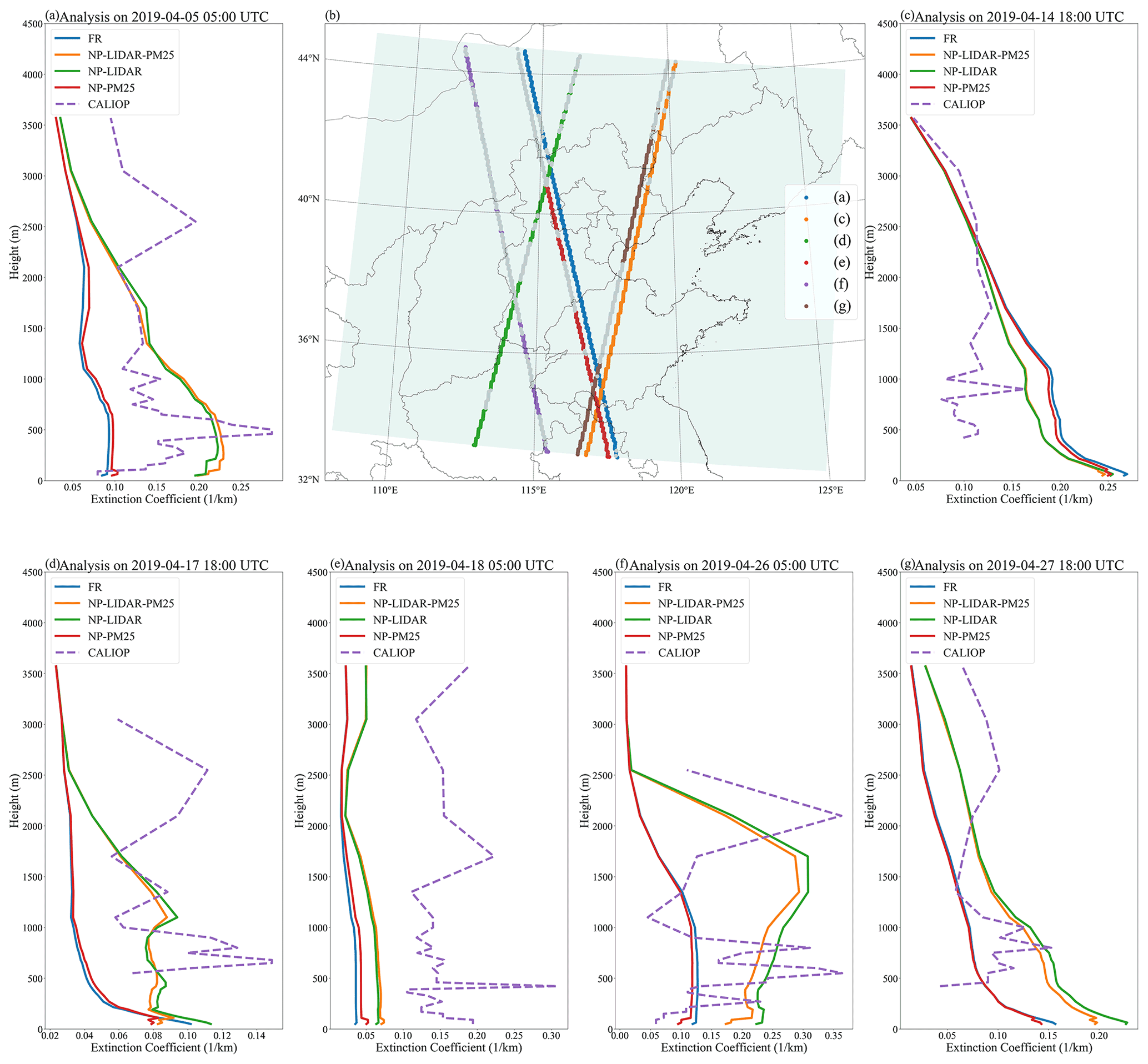
Figure 12The extinction coefficient vertical profile of CALIOP measurement and analysis of the FR, NP-PM25, NP-LIDAR, and NP-LIDAR-PM25 experiments at 05:00 UTC on 5 April 2019 (a), 18:00 UTC on 14 April 2019 (c), 18:00 UTC on 17 April 2019 (d), 05:00 UTC on 18 April 2019 (e), 05:00 UTC on 26 April 2019 (f), and 18:00 UTC on 27 April 2019 (g). The CALIPSO orbit paths are also shown (b). The shaded area denotes the model domain, and the gray lines (b) denote the part of orbits with missing extinction coefficient data through the vertical profile.
Apart from spaceborne lidar measurements, ground-based AOD measurements are also utilized to independently evaluate the performance of the NAQPMS-PDAF, especially assimilating ground-based lidar measurements. The number of AERONET sites is more than 700 around the world, and AERONET measurements are widely used. While only the AOD measurements are from the four AERONET sites, the evaluation based on these sites is still a preliminary reference to the performance of the NAQPMS-PDAF. Figure 13 shows the time series of comparison between AERONET AODs and the AODs calculated from the analysis and forecast in the four experiments in this study. The locations of these four sites shown in Fig. 13 are approximately concentrated in Beijing. Referring to the spatial distribution of ground-based lidar shown in Fig. 3, these four AERONET sites are mainly affected by the DA lidar of no. 10 in Langfang, as well as some adjacent surface PM2.5 measurements. Due to the relatively close distance, the DA performance of the NAQPMS-PDAF is similar over these four AERONET sites. Taking the Beijing-PKU (Peking University) site as an example, the AOD measurements show diurnal variability with high AOD at night and relatively low AOD in the daytime (Fig. 13a). The FR and NP-PM25 experiments have good consistency with the AOD measurements when AODs are less than 0.5. However, an AOD underestimation can be identified in the FR and NP-PM25 experiments during the period with relatively high AODs (>1.0), such as the period from 12:00 LST (local standard time) on 21 April 2019 to 12:00 LST on 24 April 2019. The simulations (analysis and forecast) in the NP-LIDAR and NP-LIDAR-PM25 experiments generally agree well with the AERONET AOD measurements, which can capture the relatively high AODs (such as the period from 12:00 LST on 21 April 2019 to 12:00 LST on 24 April 2019) and low AODs (such as the period from 12:00 LST on 6 April 2019 to 12:00 LST on 8 April 2019.). In summary, the AOD simulations have a more consistent pattern with the AERONET AOD after assimilating ground-based lidar measurements including aerosol vertical information, while only assimilating surface measurements has no such advantages.
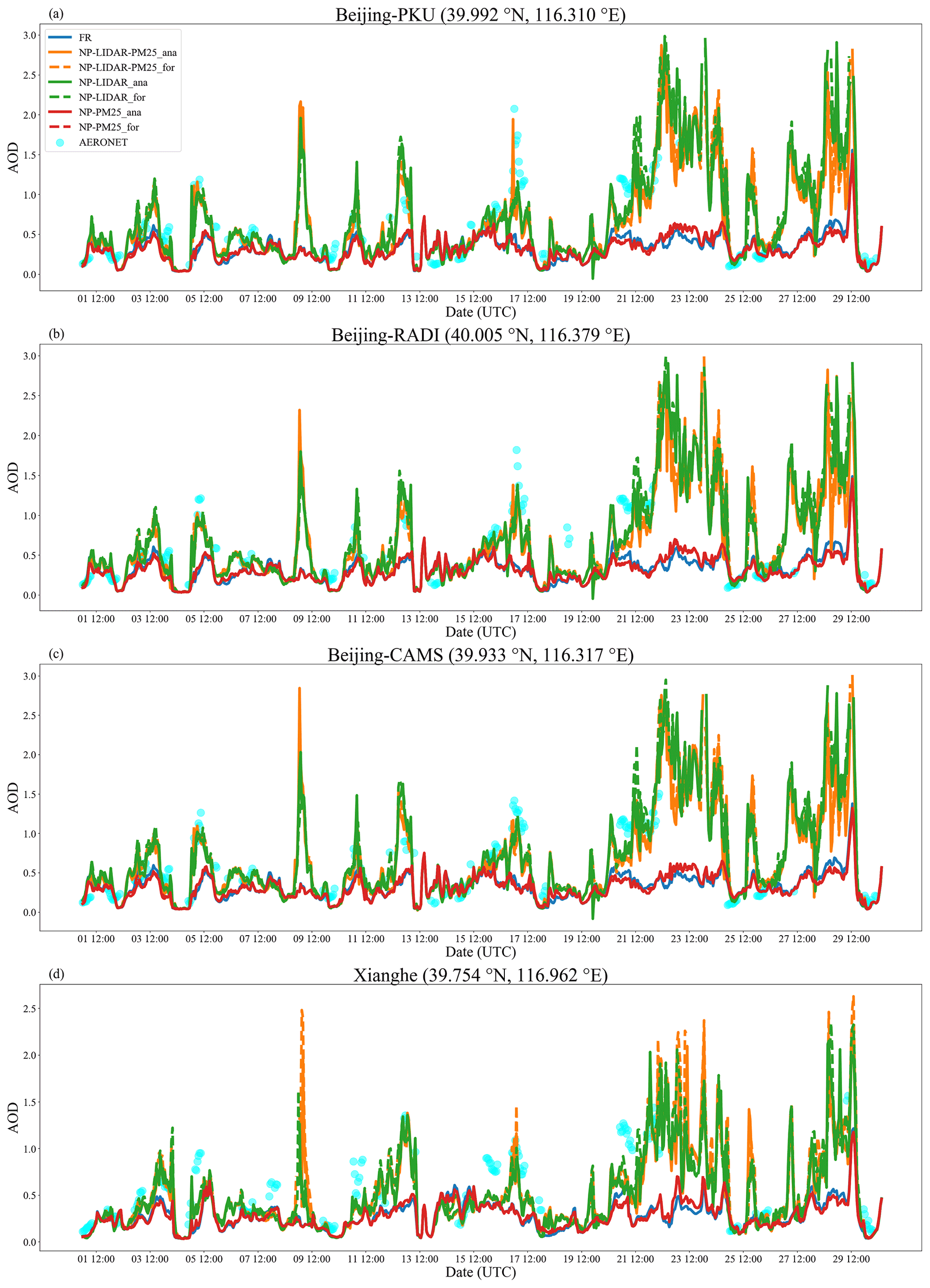
Figure 13Hourly time series of AOD measured by AERONET and in the analysis and forecast of the FR, NP-PM25, NP-LIDAR, and NP-LIDAR-PM25 experiments at the AERONET sites Beijing-PKU (a), Beijing-RADI (Institute of Remote Sensing and Digital Earth) (b), Beijing-CAMS (Chinese Academy of Meteorological Sciences) (c), and Xianghe (d).
3.3 Vertical profile analysis
Figure 14 shows the vertical distribution of aerosol extinction coefficients averaged over DA sites and VE sites, respectively, in which the vertical profiles of extinction coefficients measured by ground-based lidar (red line) are the output after vertical interpolation. The difference in vertical profiles averaged over DA sites between the FR and NP-PM25 experiments in the analysis can be found only near the surface with slightly small extinction coefficients in the NP-PM25 experiment (Fig. 14a). This suggests that the assimilation of surface PM2.5 measurements can only affect the first layer of the model, as well as the above two layers under the impact of vertical correlation length, and has limited influence on the entire aerosol vertical distribution, which is an inducement to assimilate measurements, including aerosol vertical information, to improve the aerosol vertical profile simulations. The aerosol extinction coefficients decrease with height in the FR and NP-PM25 experiments, which show large discrepancies compared with the ground-based lidar measurements, especially from 400 to 1000 m. The discrepancies of aerosol extinction coefficients between the FR (NP-PM25) and NP-LIDAR (NP-LIDAR-PM25) experiments (negative increments) occur at a height of approximately 5000 m, which corresponds to the top height (5235 m) of ground-based lidar measurements assimilated. The extinction coefficients are relatively small at a height of approximately 5000 m in the FR experiment due to a lack of aerosol loading. The negative increments of extinction coefficients between the FR (NP-PM25) and NP-LIDAR (NP-LIDAR-PM25) experiments, namely, the difference of extinction coefficients, are gradually improved with decreasing height. The most significant improvement occurs at a height of approximately 400 m with extinction coefficients of 0.37 km−1, where the extinction reaches the highest value. The extinction coefficients in the analysis then decrease with decreasing height until a height of 300 m, which is the blind zone height in the NP-LIDAR and NP-LIDAR-PM25 experiments. The discrepancies in aerosol extinction coefficients between the NP-LIDAR and NP-LIDAR-PM25 experiments occur below the lidar blind zone height, in which the extinction coefficients in NP-LIDAR sharply increase and those in the NP-LIDAR-PM25 decrease with the decreasing height. The extinction coefficients near the surface in the NP-LIDAR-PM25 experiment are closer to those in the NP-PM25 experiment than those in the NP-LIDAR experiment. Note that the surface PM2.5 simulations in NP-PM25 are superior to those in the NP-LIDAR experiment, which has been evaluated in Sect. 3.2.1 and 3.2.2. Therefore, the discrepancies are due to the NP-LIDAR-PM25 experiment assimilating the surface PM2.5 measurement, which makes the aerosol vertical profiles more consistent with the measurements than those in the NP-LIDAR experiment near the surface. The aerosol vertical profile in the analysis in NP-LIDAR-PM25 combines the model output and lidar measurements with the minimum uncertainty (orange line in Fig. 14a), showing aerosol loading at high elevations of approximately 500 m. As shown in Fig. 14b, the difference in extinction coefficients in the 1 h forecast between the FR and NP-PM25 decreases more than that in the analysis (Fig. 14a). The consistency between the forecast and lidar measurements degrades within 1 model hour simulation at a height of approximately 700 m. The variability in the forecast is probably due to the attenuation of the impact of DA during the model simulation. The pattern of the vertical profile in the forecast is similar to that in the analysis in the NP-LIDAR experiment. The near-surface part of the aerosol vertical profile in the NP-LIDAR-PM25 experiment is close to that in the NP-LIDAR experiment. This suggests that the temporal effect of assimilating the surface PM2.5 measurements is weaker than that of assimilating the ground-based lidar measurements. The aerosol vertical profile from lidar measurements averaged over VE sites shows a similar shape to that over DA sites, indicating that the measurements at DA sites have good consistency compared with those at VE sites. The aerosol vertical profile in the NP-LIDAR (NP-LIDAR-PM25) experiment shows good consistency with that in the lidar measurement above a height of approximately 500 m, of which the peak extinction value has a discrepancy below that height. The decreasing gradients of extinction coefficients at VE sites from a height of approximately 500 m to the blind zone are steeper than those at DA sties. This indicates that the peak height becomes low with the attenuation of the impact of DA. Combined with the attenuation of the impact of surface DA, a particular break occurs near the surface in the NP-LIDAR-PM25 experiment (Fig. 14c). The difference in extinction coefficients between the analysis and forecast at VE sites is similar to that at DA sites. Following Su et al. (2020), aerosol vertical structures can be largely classified into three types: well-mixed, decreasing with height, and inverse structures. The shape of the vertical structure is totally changed from decreasing with height in the FR experiment to inverse structures in the NP-LIDAR and NP-LIDAR-PM25 experiments, which may affect the vertical distribution of aerosol radiative forcing (Z. Li et al., 2017; Su et al., 2020) and is not the focus of this study.
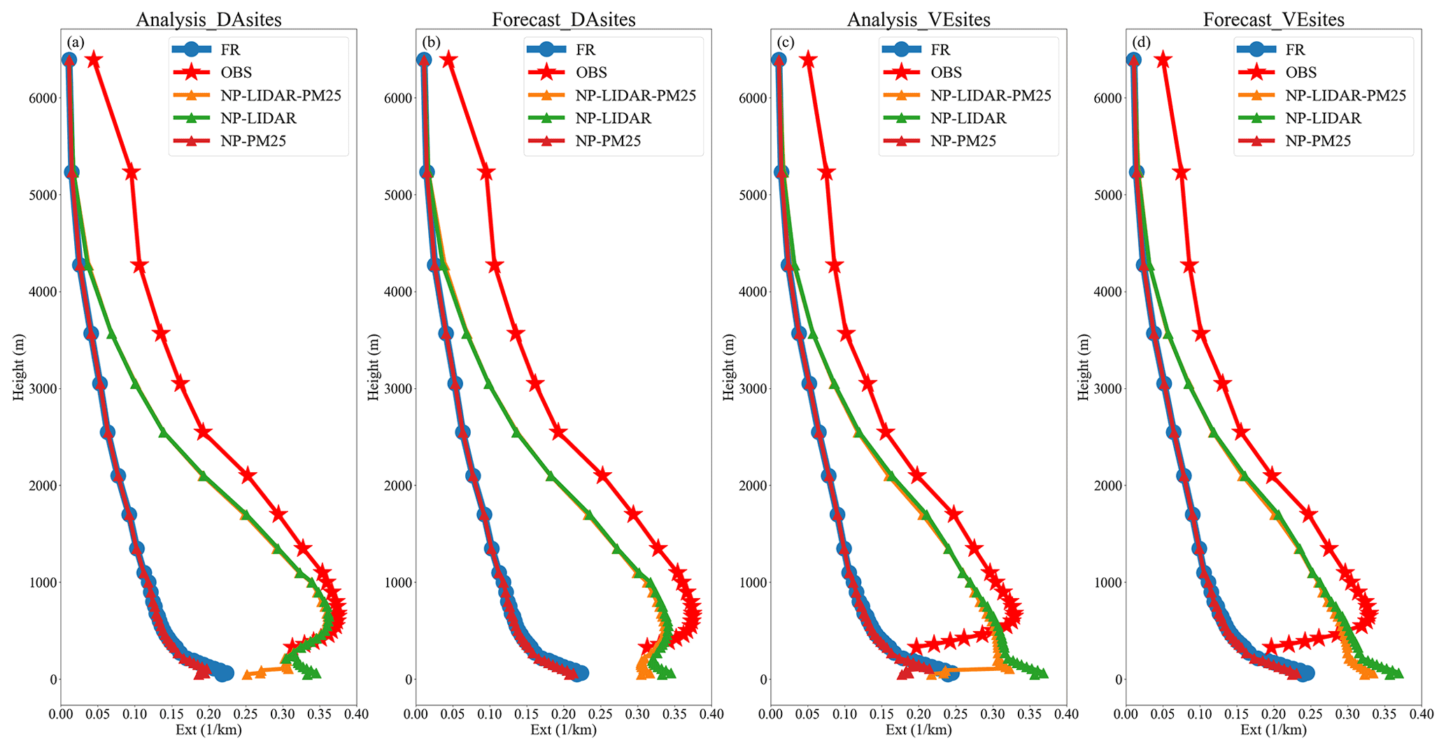
Figure 14Vertical distribution of aerosol extinction coefficients in the analysis averaged among DA sites (a), forecast averaged among DA sites (b), analysis averaged among VE sites (c), and forecast averaged among VE sites (d) in the FR, NP-PM25, NP-LIDAR, and NP-LIDAR-PM25 experiments and ground-based lidar measurements.
3.4 Uncertainties
The heart of DA is dealing with uncertainty (Bannister, 2017). The ensemble members can provide error information in ensemble-based DA. The analysis ensemble spread, estimated as the standard deviation of the simulations across the ensemble, can be used as an indicator of the analysis uncertainty on the estimated observations mapped by the state vectors in the ensemble-based DA framework (Arellano et al., 2007; Miyazaki et al., 2012). The analysis uncertainty is concerned with errors in input data such as emissions, the representation of physical and chemical processes in numerical models, assimilated measurements, and so on (Miyazaki et al., 2020). The ensemble spread of extinction coefficients simulated across the 20 ensemble members in the FR and NP-LIDAR-PM25 experiments is shown in Fig. 15, and the height from the surface to 1700 m is divided into three bins (50, 64 to 502 m, and 550 to 1700 m) to present different characteristics of uncertainty. The color scale bar is set to the same height bin and is different at the different height bins. The analysis spread in FR at 50 m (considered the surface in the model) is mainly characterized by a large spread in a few point source regions due to perturbations in emissions (Fig. 15b). The direct effect (assimilating surface measurement) and indirect effect (assimilating ground-based lidar measurement) of posterior fields after DA reduce the uncertainty represented by the analysis spread in the NP-LIDAR-PM25 experiment, which is vividly shown in Fig. 15c. The ensemble spread in the FR experiment shows a combination of emission-related and transport-related uncertainties from 64 to 502 m (Fig. 15d). We see changes in the structure of the ensemble spread in NP-LIDAR-PM25, with clear indications of a reduction in uncertainties (Fig. 15e). The analysis spread with uniform spatial distribution averaged from heights of 550 to 1700 m is less affected by surface emissions and more affected by transport-related uncertainties, such as horizontal advection in the FR experiment (Fig. 15f). The average analysis ensemble spread from 550 to 1700 m over the middle and southern NCP, which is the coverage area of lidar DA, is significantly reduced in the NP-LIDAR-PM25 experiment (Fig. 15g). The average profiles of the analysis spread are calculated from the surface to a height of 3570 m in the FR and NP-LIDAR-PM25 experiments, which are shown in Fig. 15a. As is described in Sect. 2.3.3, emission which is one of significant input of NAQPMS-PDAF is the unique perturbed source of initial conditions. However, most kinds of emissions concentrated around the surface and a few kinds of emissions (emission from industry, power plant and biomass burning) can emit primary PM2.5 and its precursors at a certain altitude. As a result, the ensemble spread decreases with height in the FR experiment. It means that the analysis increment of each assimilation cycle tends to apportion more aerosol concentration near the surface. The reduction of the ensemble spread occurs at a height of approximately 2500 m and increases with decreasing height (Fig. 15a). It demonstrates that the analysis of ensemble filter after assimilating ground-based lidar measurements converges to a true state.
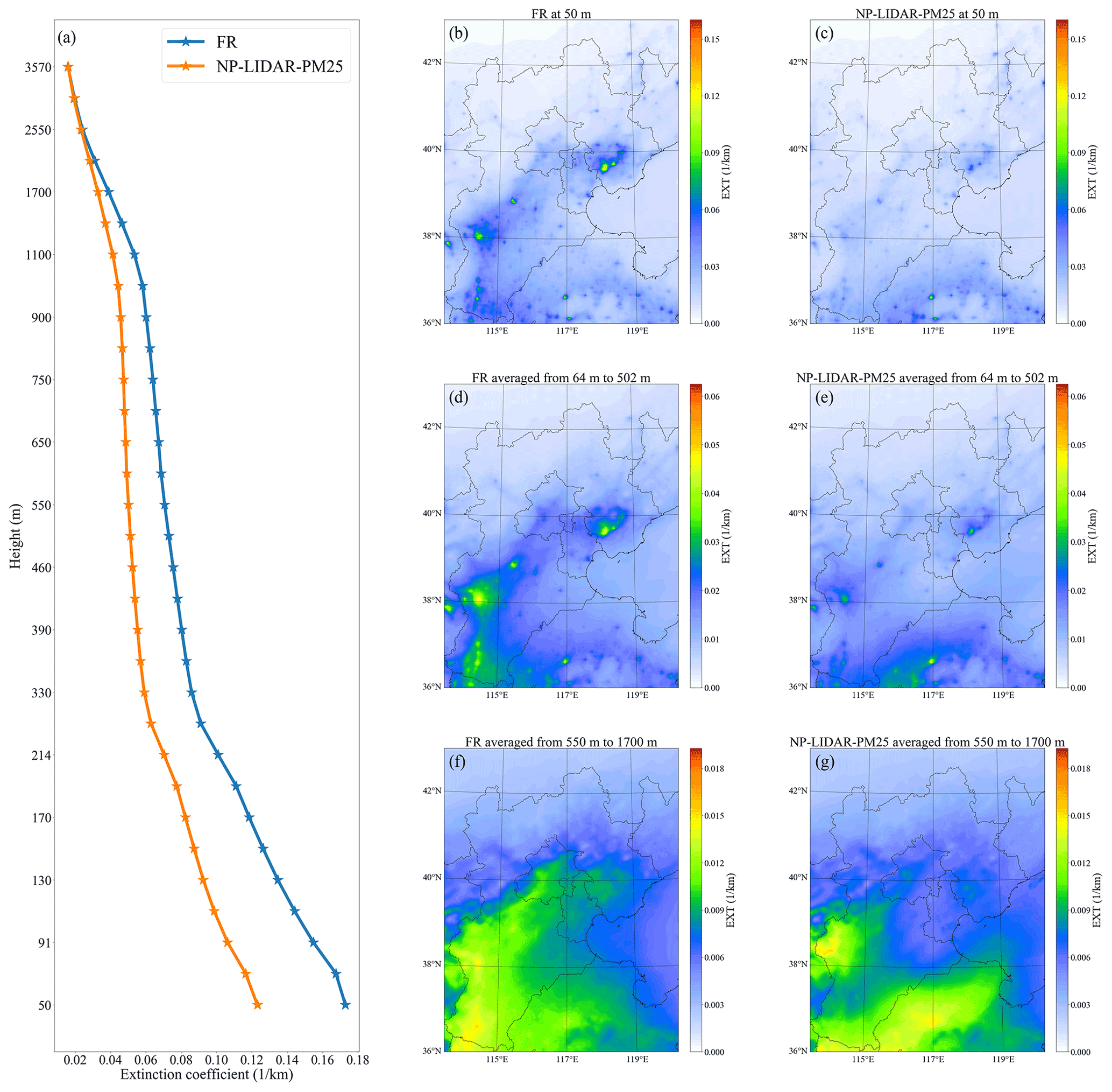
Figure 15Vertical profile of the analysis ensemble spread of extinction coefficients averaged among DA sites in the FR and NP-LIDAR-PM25 experiments (a). The spatial distribution of the analysis ensemble spread of extinction coefficients at 50 m in the FR experiment (b), at 50 m in NP-LIDAR-PM25 (c), averaged from 64 to 502 m in FR (d), averaged from 64 to 502 m in NP-LIDAR-PM25 (e), averaged from 550 to 1700 m in FR (f), and averaged from 550 to 1700 m in NP-LIDAR-PM25. All results are averaged over 1–30 April 2019.
In this paper, we couple the atmospheric chemistry-transport model NAQPMS with the PDAF online for the first time to establish a high-performance ensemble filter system (NAQPMS-PDAF) to mainly investigate the impact of assimilating measurements, including aerosol vertical information. We examine the computational efficiency and DA performance of the NAQPMS-PDAF on the analysis and subsequent 1 h simulations after assimilating 1-month-long aerosol extinction coefficient profiles measured by five ground-based lidars (six ground-based lidar measurements are used as evaluation) during April 2019 and the concurrent hourly surface PM2.5 measurements over the NCP with four experiments (FR, NP-PM25, NP-LIDAR, and NP-LIDAR-PM25). Except for the lidar and surface PM2.5 measurements, which are not assimilated, the AERONET AODs and the vertical profiles of extinction coefficients measured by the CALIOP are utilized as independent validations. The characteristics of aerosol vertical profiles and the uncertainties in the NAQPMS-PDAF are also probed in detail.
The coupling between the NAQPMS and PDAF is implemented in a fully integrated fashion with data exchange performed via main memory, which avoids frequently reading and writing model restart files. Two levels of parallelization are introduced to perform ensemble simulations running fully parallel and to implement the filter algorithm efficiently. The arrangement of the dimensional order of state vectors during the ensemble filter is especially designed to allow the submatrix to cut along the longitudinal direction with each slice containing full variable information.
The scaling tests on the massively parallel HPC BDCSIP are performed first, where the strong scaling shows that 50 processors per model realization is the optimal configuration synthetically considering strong scaling efficiency and the increment in computational load, and the weak scaling reveals that the NAQPMS-PDAF runs efficiently with the number of processors from 100 to 2500 with the weak scaling efficiency only decreasing from 1.0 to 0.7. This scaling study indicates that online coupling works very well in a technical sense. The ensemble performance is then evaluated on which all the following results depend. The NAQPMS-PDAF is well balanced near the surface and shows a slightly insufficient spread at high altitude due to the disturbed emissions mainly near the surface, which is evaluated by the ensemble members.
The numerical model without DA has deficiencies in reproducing pollutant plumes, especially inside the boundary layer, which shows an obvious underestimation in the FR experiment that commonly exists in other CTMs. Compared with the assimilated ground-based lidar measurements as internal checks, the underestimation of the aerosol extinction coefficients is remarkably improved in the analysis of NP-LIDAR and NP-LIDAR-PM25 experiments with the BIAS changing from −0.20 to −0.02 km−1, and the correlation coefficients increasing from 0.33 to 0.91 averaged at sites with DA. The statistical performance in the subsequent 1 h simulation is always slightly weaker than that in the analysis due to the attenuation of the impact of DA. Only assimilating surface measurements can directly improve the surface PM2.5 simulations but has limited influence on high elevations. However, only assimilating ground-based lidar measurements can mainly improve the surface PM2.5 simulations with a slightly weaker performance than that in assimilating surface PM2.5 measurements. In one word, the performance of the NAQPMS-PDAF to simulate surface PM2.5 in assimilating surface PM2.5 measurements, ground-based lidar measurements, and both of these measurements is better than that in the FR experiment. These results indicate that the NAQPMS-PDAF system operates successfully.
In the independent validation of lidar measurements, the qualitative attenuation is weaker than the quantitative attenuation after assimilating measurements, including aerosol vertical information, when comparing the performance on the forecast at DA sites with that on the analysis at VE sites. The lidar measurements assimilated indeed include authentic vertical distribution information of aerosols, and the NP-LIDAR experiment can notably improve the aerosol vertical distribution simulations and then improve the surface PM2.5 simulations in the numerical model, but the quantification, especially on the surface PM2.5 mass concentration, needs to be strengthened. The aerosol extinction coefficients measured by the CALIOP, which has sparse coverage and limited data integrity, are utilized as independent evaluations, and it is found that assimilating ground-based lidar can significantly improve both the overestimation and underestimation of the extinction values, especially below approximately 2000 m. AODs measured by the four AERONET sites, which are approximately concentrated in Beijing, are also used to independently validate the performance. Lidar DA can have a more consistent pattern with the AERONET measurements, while only assimilating surface measurements has no such advantages.
In the vertical profile analysis, the aerosol extinction coefficients decrease with height in the FR and NP-PM25 experiments, which presents large discrepancies compared with the ground-based lidar measurements, especially from 400 to 1000 m.
The negative increments of extinction coefficients between the FR (NP-PM25) and NP-LIDAR (NP-LIDAR-PM25) experiments gradually improve with decreasing height. The most significant improvement occurs at a height of approximately 400 m with extinction coefficients of 0.37 km−1, where the extinction reaches the highest value. Although assimilating surface PM2.5 measurements has a limited impact on the aerosol vertical profile, the correction in the NP-LIDAR-PM25 experiment occurs near the surface and makes the aerosol vertical profiles more consistent with the measurements than those in the NP-LIDAR experiment. Assimilating ground-based lidar measurements can have a larger temporal impact than assimilating surface measurements. In addition, the height of the peak extinction coefficient value decreases within the 1 h forecast due to the attenuation of the impact of DA.
Finally, the uncertainties of the NAQPMS-PDAF are examined. The direct impact (assimilating surface PM2.5 measurement) and indirect impact (assimilating ground-based lidar measurements) of posterior fields after DA reduce the uncertainty represented by the analysis spread in the NP-LIDAR-PM25 experiment, which is the emission-related ensemble spread at 50 m, and a combination of emission-related and transport-related ensemble spreads averages from 64 to 502 m, and the transport-related ensemble spread averages from 550 to 1700 m. It demonstrates that the analysis of ensemble filter after assimilating ground-based lidar measurements converges to a true state.
The proposed NAQPMS-PDAF can significantly improve the aerosol vertical profile simulations and has a large potential to allow further study of the impact of aerosol vertical distribution. In future work, we plan to investigate the key factors mainly impacting the surface PM2.5 simulations after assimilating measurements, including vertical information, as the performance of lidar assimilation in this study shows a limited positive influence on the surface PM2.5 simulations. We also plan to further expand the state vectors, and the measurements assimilated as the NAQPMS-PDAF is a modularized DA system with good extendibility. This will allow us to jointly assimilate surface, ground-based, and spaceborne measurements for a better three-dimensional characterization of aerosol components, as well as gaseous pollutants such as SO2, NOx, and CO.
The source codes, observation data, and model output in our work are available online via Zenodo (https://doi.org/10.5281/zenodo.6344181, Wang and Yang, 2021).
The supplement related to this article is available online at: https://doi.org/10.5194/gmd-15-3555-2022-supplement.
HW implemented PDAF with NAQPMS, performed numerical experiments, and carried out the analysis. TY provided scientific guidance for the article design. TY, ZW, and XC provided valuable suggestions for this article. JL, WC, and GT provided lidar and surface PM2.5 data. LK provided the code of perturbing the initial emissions. XC provided help for the model code. HW wrote the paper and all listed authors have read and approved the final paper.
The contact author has declared that neither they nor their co-authors have any competing interests.
Publisher's note: Copernicus Publications remains neutral with regard to jurisdictional claims in published maps and institutional affiliations.
Ting Yang gratefully acknowledges the Program of the Youth Innovation Promotion Association (CAS). We thank the Big Data Cloud Service Infrastructure Platform (BDCSIP) for providing computing resources. This research is supported by the National Key Scientific and Technological Infrastructure project “Earth System Science Numerical Simulator Facility”. We thank the anonymous reviewers for their constructive suggestions that helped improve the paper.
This research has been supported by the Strategic Priority Research Program of the Chinese Academy of Sciences (grant no. XDA19040203), the National High Technology Research and Development Program of China (grant no. 2019YFC214802), and the Young Talent Project of the Center for Excellence in Regional Atmospheric Environment, CAS (grant no. CERAE201803).
This paper was edited by Xiaomeng Huang and reviewed by two anonymous referees.
Alfeld, P.: A trivariate clough–tocher scheme for tetrahedral data, Comput. Aided Geom. Des., 1, 169–181, https://doi.org/10.1016/0167-8396(84)90029-3, 1984.
Anderson, J., Hoar, T., Raeder, K., Liu, H., Collins, N., Torn, R., and Avellano, A.: The Data Assimilation Research Testbed: A Community Facility, B. Am. Meteorol. Soc., 90, 1283–1296, https://doi.org/10.1175/2009BAMS2618.1, 2009.
Anderson, J. L. and Anderson, S. L.: A Monte Carlo Implementation of the Nonlinear Filtering Problem to Produce Ensemble Assimilations and Forecasts, Mon. Weather Rev., 127, 2741–2758, https://doi.org/10.1175/1520-0493(1999)127<2741:AMCIOT>2.0.CO;2, 1999.
Arellano Jr., A. F., Raeder, K., Anderson, J. L., Hess, P. G., Emmons, L. K., Edwards, D. P., Pfister, G. G., Campos, T. L., and Sachse, G. W.: Evaluating model performance of an ensemble-based chemical data assimilation system during INTEX-B field mission, Atmos. Chem. Phys., 7, 5695–5710, https://doi.org/10.5194/acp-7-5695-2007, 2007.
Athanasopoulou, E., Tombrou, M., Pandis, S. N., and Russell, A. G.: The role of sea-salt emissions and heterogeneous chemistry in the air quality of polluted coastal areas, Atmos. Chem. Phys., 8, 5755–5769, https://doi.org/10.5194/acp-8-5755-2008, 2008.
Bahreini, R.: Aircraft-based aerosol size and composition measurements during ACE-Asia using an Aerodyne aerosol mass spectrometer, J. Geophys. Res., 108, 8645, https://doi.org/10.1029/2002JD003226, 2003.
Bai, D., Wang, H., Cheng, M., Gao, W., Yang, Y., Huang, W., Ma, K., Zhang, Y., Zhang, R., Zou, J., Wang, J., Liang, Y., Li, N., and Wang, Y.: Source apportionment of PM2.5 and its optical properties during a regional haze episode over north China plain, Atmos. Pollut. Res., 12, 89–99, https://doi.org/10.1016/j.apr.2020.08.023, 2021.
Bannister, R. N.: A review of operational methods of variational and ensemble-variational data assimilation: Ensemble-variational Data Assimilation, Q. J. Roy. Meteor. Soc., 143, 607–633, https://doi.org/10.1002/qj.2982, 2017.
Baracchini, T., Chu, P. Y., Šukys, J., Lieberherr, G., Wunderle, S., Wüest, A., and Bouffard, D.: Data assimilation of in situ and satellite remote sensing data to 3D hydrodynamic lake models: a case study using Delft3D-FLOW v4.03 and OpenDA v2.4, Geosci. Model Dev., 13, 1267–1284, https://doi.org/10.5194/gmd-13-1267-2020, 2020.
Barker, D., Huang, X.-Y., Liu, Z., Auligné, T., Zhang, X., Rugg, S., Ajjaji, R., Bourgeois, A., Bray, J., Chen, Y., Demirtas, M., Guo, Y.-R., Henderson, T., Huang, W., Lin, H.-C., Michalakes, J., Rizvi, S., and Zhang, X.: The Weather Research and Forecasting Model's Community Variational/Ensemble Data Assimilation System: WRFDA, B. Am. Meteorol. Soc., 93, 831–843, https://doi.org/10.1175/BAMS-D-11-00167.1, 2012.
Bishop, C. H. and Toth, Z.: Ensemble Transformation and Adaptive Observations, J. Atmos. Sci., 56, 1748–1765, https://doi.org/10.1175/1520-0469(1999)056<1748:ETAAO>2.0.CO;2, 1999.
Bocquet, M.: Parameter-field estimation for atmospheric dispersion: application to the Chernobyl accident using 4D-Var, Q. J. Roy. Meteor. Soc., 138, 664–681, https://doi.org/10.1002/qj.961, 2012.
Bocquet, M., Elbern, H., Eskes, H., Hirtl, M., Žabkar, R., Carmichael, G. R., Flemming, J., Inness, A., Pagowski, M., Pérez Camaño, J. L., Saide, P. E., San Jose, R., Sofiev, M., Vira, J., Baklanov, A., Carnevale, C., Grell, G., and Seigneur, C.: Data assimilation in atmospheric chemistry models: current status and future prospects for coupled chemistry meteorology models, Atmos. Chem. Phys., 15, 5325–5358, https://doi.org/10.5194/acp-15-5325-2015, 2015.
Brasseur, G. P., Hauglustaine, D. A., Walters, S., Rasch, P. J., Müller, J.-F., Granier, C., and Tie, X. X.: MOZART, a global chemical transport model for ozone and related chemical tracers: 1. Model description, J. Geophys. Res., 103, 28265–28289, https://doi.org/10.1029/98JD02397, 1998.
Burgers, G.: Analysis Scheme in the Ensemble Kalman Filter, Mon. Weather Rev., 126, 1719–1724, https://doi.org/10.1175/1520-0493(1998)126<1719:ASITEK>2.0.CO;2, 1998.
Byun, W. and Dennis, R.: Design artifacts in eulerian air quality models: Evaluation of the effects of layer thickness and vertical profile correction on surface ozone concentrations, Atmos. Environ., 1, 105–126, https://doi.org/10.1016/1352-2310(94)00225-A, 1995.
Chai, T. and Draxler, R. R.: Root mean square error (RMSE) or mean absolute error (MAE)? – Arguments against avoiding RMSE in the literature, Geosci. Model Dev., 7, 1247–1250, https://doi.org/10.5194/gmd-7-1247-2014, 2014.
Chen, Y., Zhao, C., Zhang, Q., Deng, Z., Huang, M., and Ma, X.: Aircraft study of Mountain Chimney Effect of Beijing, China, J. Geophys. Res., 114, D08306, https://doi.org/10.1029/2008JD010610, 2009.
Chen, Z., Liu, J., Song, M., Yang, Q., and Xu, S.: Impacts of Assimilating Satellite Sea Ice Concentration and Thickness on Arctic Sea Ice Prediction in the NCEP Climate Forecast System, J. Climate, 30, 8429–8446, https://doi.org/10.1175/JCLI-D-17-0093.1, 2017.
Cheng, X., Liu, Y., Xu, X., You, W., Zang, Z., Gao, L., Chen, Y., Su, D., and Yan, P.: Lidar data assimilation method based on CRTM and WRF-Chem models and its application in PM2.5 forecasts in Beijing, Sci. Total Environ., 682, 541–552, https://doi.org/10.1016/j.scitotenv.2019.05.186, 2019.
Cheng, Y., Dai, T., Goto, D., Schutgens, N. A. J., Shi, G., and Nakajima, T.: Investigating the assimilation of CALIPSO global aerosol vertical observations using a four-dimensional ensemble Kalman filter, Atmos. Chem. Phys., 19, 13445–13467, https://doi.org/10.5194/acp-19-13445-2019, 2019.
Donahue, N. M., Robinson, A. L., Stanier, C. O., and Pandis, S. N.: Coupled Partitioning, Dilution, and Chemical Aging of Semivolatile Organics, Environ. Sci. Technol., 40, 2635–2643, https://doi.org/10.1021/es052297c, 2006.
Eck, T. F., Holben, B. N., Reid, J. S., Dubovik, O., Smirnov, A., O'Neill, N. T., Slutsker, I., and Kinne, S.: Wavelength dependence of the optical depth of biomass burning, urban, and desert dust aerosols, J. Geophys. Res., 104, 31333–31349, https://doi.org/10.1029/1999JD900923, 1999.
Emili, E., Barret, B., Le Flochmoën, E., and Cariolle, D.: Comparison between the assimilation of IASI Level 2 ozone retrievals and Level 1 radiances in a chemical transport model, Atmos. Meas. Tech., 12, 3963–3984, https://doi.org/10.5194/amt-12-3963-2019, 2019.
Evensen, G.: Sequential data assimilation with a nonlinear quasi-geostrophic model using Monte Carlo methods to forecast error statistics, J. Geophys. Res., 99, 10143–10162, https://doi.org/10.1029/94JC00572, 1994.
Evensen, G.: Data Assimilation: The Ensemble Kalman Filter, 2nd edn., Springer-Verlag, https://doi.org/10.1007/978-3-642-03711-5, 2009.
Fan, W., Qin, K., Xu, J., Yuan, L., Li, D., Jin, Z., and Zhang, K.: Aerosol vertical distribution and sources estimation at a site of the Yangtze River Delta region of China, Atmos. Res., 217, 128–136, https://doi.org/10.1016/j.atmosres.2018.11.002, 2019.
Feng, S., Jiang, F., Wu, Z., Wang, H., Ju, W., and Wang, H.: CO Emissions Inferred from Surface CO Observations over China in December 2013 and 2017, J. Geophys. Res.-Atmos., 125, e2019JD031808, https://doi.org/10.1029/2019JD031808, 2020.
Garcia, M., Ramirez, I., Verlaan, M., and Castillo, J.: Application of a three-dimensional hydrodynamic model for San Quintin Bay, B.C., Mexico. Validation and calibration using OpenDA, J. Comput. Appl. Math., 273, 428–437, https://doi.org/10.1016/j.cam.2014.05.003, 2015.
Gaspari, G. and Cohn, S. E.: Construction of correlation functions in two and three dimensions, Q. J. Roy. Meteor. Soc., 125, 723–757, https://doi.org/10.1002/qj.49712555417, 1999.
Gebler, S., Kurtz, W., Pauwels, V. R. N., Kollet, S. J., Vereecken, H., and Hendricks Franssen, H.-J.: Assimilation of High-Resolution Soil Moisture Data Into an Integrated Terrestrial Model for a Small-Scale Head-Water Catchment, Water Resour. Res., 55, 10358–10385, https://doi.org/10.1029/2018WR024658, 2019.
Gillet-Chaulet, F.: Assimilation of surface observations in a transient marine ice sheet model using an ensemble Kalman filter, The Cryosphere, 14, 811–832, https://doi.org/10.5194/tc-14-811-2020, 2020.
Gimmestad, G., Forrister, H., Grigas, T., and O'Dowd, C.: Comparisons of aerosol backscatter using satellite and ground lidars: implications for calibrating and validating spaceborne lidar, Sci. Rep., 7, 42337, https://doi.org/10.1038/srep42337, 2017.
Gropp, W., Lust, E., and Skjellum, A.: Using MPI: Portable Parallel Programming with the Message Passing Interface, 2nd edn., The MIT Press, Cambridge, Massachusetts, ISBN 978-0-262-25628-5, https://doi.org/10.7551/mitpress/7056.001.0001, 1994.
Ha, S., Liu, Z., Sun, W., Lee, Y., and Chang, L.: Improving air quality forecasting with the assimilation of GOCI aerosol optical depth (AOD) retrievals during the KORUS-AQ period, Atmos. Chem. Phys., 20, 6015–6036, https://doi.org/10.5194/acp-20-6015-2020, 2020.
Hauglustaine, D. A., Brasseur, G. P., Walters, S., Rasch, P. J., Müller, J.-F., Emmons, L. K., and Carroll, M. A.: MOZART, a global chemical transport model for ozone and related chemical tracers: 2. Model results and evaluation, J. Geophys. Res., 103, 28291–28335, https://doi.org/10.1029/98JD02398, 1998.
Holben, B. N., Eck, T. F., Slutsker, I., Tanré, D., Buis, J. P., Setzer, A., Vermote, E., Reagan, J. A., Kaufman, Y. J., Nakajima, T., Lavenu, F., Jankowiak, I., and Smirnov, A.: AERONET – A Federated Instrument Network and Data Archive for Aerosol Characterization, Remote Sens. Environ., 66, 1–16, https://doi.org/10.1016/S0034-4257(98)00031-5, 1998.
Holben, B. N., Tanré, D., Smirnov, A., Eck, T. F., Slutsker, I., Abuhassan, N., Newcomb, W. W., Schafer, J. S., Chatenet, B., Lavenu, F., Kaufman, Y. J., Castle, J. V., Setzer, A., Markham, B., Clark, D., Frouin, R., Halthore, R., Karneli, A., O'Neill, N. T., Pietras, C., Pinker, R. T., Voss, K., and Zibordi, G.: An emerging ground-based aerosol climatology: Aerosol optical depth from AERONET, J. Geophys. Res., 106, 12067–12097, https://doi.org/10.1029/2001JD900014, 2001.
Houtekamer, P. L. and Zhang, F.: Review of the Ensemble Kalman Filter for Atmospheric Data Assimilation, Mon. Weather Rev., 144, 4489–4532, https://doi.org/10.1175/MWR-D-15-0440.1, 2016.
Houtekamer, P. L., Mitchell, H. L., Pellerin, G., Buehner, M., Charron, M., Spacek, L., and Hansen, B.: Atmospheric Data Assimilation with an Ensemble Kalman Filter: Results with Real Observations, Mon. Weather Rev., 133, 604–620, https://doi.org/10.1175/MWR-2864.1, 2005.
Hunt, B. R., Kostelich, E. J., and Szunyogh, I.: Efficient data assimilation for spatiotemporal chaos: A local ensemble transform Kalman Filter, Physica D, 230, 112–126, https://doi.org/10.1016/j.physd.2006.11.008, 2007.
Kalman, R. E. and Bucy, R. S.: New results in linear filtering and prediction theory, J. Fluids Eng., 83, 95–108, https://doi.org/10.1115/1.3658902, 1961.
Kipling, Z., Stier, P., Johnson, C. E., Mann, G. W., Bellouin, N., Bauer, S. E., Bergman, T., Chin, M., Diehl, T., Ghan, S. J., Iversen, T., Kirkevåg, A., Kokkola, H., Liu, X., Luo, G., van Noije, T., Pringle, K. J., von Salzen, K., Schulz, M., Seland, Ø., Skeie, R. B., Takemura, T., Tsigaridis, K., and Zhang, K.: What controls the vertical distribution of aerosol? Relationships between process sensitivity in HadGEM3–UKCA and inter-model variation from AeroCom Phase II, Atmos. Chem. Phys., 16, 2221–2241, https://doi.org/10.5194/acp-16-2221-2016, 2016.
Kong, L., Tang, X., Zhu, J., Wang, Z., Pan, Y., Wu, H., Wu, L., Wu, Q., He, Y., Tian, S., Xie, Y., Liu, Z., Sui, W., Han, L., and Carmichael, G.: Improved Inversion of Monthly Ammonia Emissions in China Based on the Chinese Ammonia Monitoring Network and Ensemble Kalman Filter, Environ. Sci. Technol., 53, 12529–12538, https://doi.org/10.1021/acs.est.9b02701, 2019.
Kong, L., Tang, X., Zhu, J., Wang, Z., Li, J., Wu, H., Wu, Q., Chen, H., Zhu, L., Wang, W., Liu, B., Wang, Q., Chen, D., Pan, Y., Song, T., Li, F., Zheng, H., Jia, G., Lu, M., Wu, L., and Carmichael, G. R.: A 6-year-long (2013–2018) high-resolution air quality reanalysis dataset in China based on the assimilation of surface observations from CNEMC, Earth Syst. Sci. Data, 13, 529–570, https://doi.org/10.5194/essd-13-529-2021, 2021.
Kurtz, W., He, G., Kollet, S. J., Maxwell, R. M., Vereecken, H., and Hendricks Franssen, H.-J.: TerrSysMP–PDAF (version 1.0): a modular high-performance data assimilation framework for an integrated land surface–subsurface model, Geosci. Model Dev., 9, 1341–1360, https://doi.org/10.5194/gmd-9-1341-2016, 2016.
Lahoz, W. and Errera, Q.: Data Assimilation, in: Making Sense of Observations, edited by: Lahoz, W., Khattatov, B., and Menard, R., Springer-Verlag, https://doi.org/10.1007/978-3-540-74703-1, 2010.
Lana, A., Bell, T. G., Simó, R., Vallina, S. M., Ballabrera-Poy, J., Kettle, A. J., Dachs, J., Bopp, L., Saltzman, E. S., Stefels, J., Johnson, J. E., and Liss, P. S.: An updated climatology of surface dimethlysulfide concentrations and emission fluxes in the global ocean, Global Biogeochem. Cy., 25, GB1004, https://doi.org/10.1029/2010GB003850, 2011.
Lawson, W. G. and Hansen, J. A.: Implications of Stochastic and Deterministic Filters as Ensemble-Based Data Assimilation Methods in Varying Regimes of Error Growth, Mon. Weather Rev., 132, 1966–1981, https://doi.org/10.1175/1520-0493(2004)132<1966:IOSADF>2.0.CO;2, 2004.
Li, C., Li, J., Dubovik, O., Zeng, Z.-C., and Yung, Y. L.: Impact of Aerosol Vertical Distribution on Aerosol Optical Depth Retrieval from Passive Satellite Sensors, Remote Sensing, 12, 1524, https://doi.org/10.3390/rs12091524, 2020.
Li, J., Wang, Z., Wang, X., Yamaji, K., Takigawa, M., Kanaya, Y., Pochanart, P., Liu, Y., Irie, H., Hu, B., Tanimoto, H., and Akimoto, H.: Impacts of aerosols on summertime tropospheric photolysis frequencies and photochemistry over Central Eastern China, Atmos. Environ., 45, 1817–1829, https://doi.org/10.1016/j.atmosenv.2011.01.016, 2011.
Li, J., Wang, Z., Zhuang, G., Luo, G., Sun, Y., and Wang, Q.: Mixing of Asian mineral dust with anthropogenic pollutants over East Asia: a model case study of a super-duststorm in March 2010, Atmos. Chem. Phys., 12, 7591–7607, https://doi.org/10.5194/acp-12-7591-2012, 2012.
Li, J., Yang, W., Wang, Z., Chen, H., Hu, B., Li, J., Sun, Y., and Huang, Y.: A modeling study of source–receptor relationships in atmospheric particulate matter over Northeast Asia, Atmospheric Environment, 91, 40–51, https://doi.org/10.1016/j.atmosenv.2014.03.027, 2014.
Li, J., Zhang, Y., Wang, Z., Sun, Y., Fu, P., Yang, Y., Huang, H., Li, J., Zhang, Q., Lin, C., and Lin, N.-H.: Regional Impact of Biomass Burning in Southeast Asia on Atmospheric Aerosols during the 2013 Seven South-East Asian Studies Project, Aerosol Air Qual. Res., 17, 2924–2941, https://doi.org/10.4209/aaqr.2016.09.0422, 2017.
Li, J., Chen, X., Wang, Z., Du, H., Yang, W., Sun, Y., Hu, B., Li, J., Wang, W., Wang, T., Fu, P., and Huang, H.: Radiative and heterogeneous chemical effects of aerosols on ozone and inorganic aerosols over East Asia, Sci. Total Environ., 622–623, 1327–1342, https://doi.org/10.1016/j.scitotenv.2017.12.041, 2018.
Li, J., Han, Z., Wu, Y., Xiong, Z., Xia, X., Li, J., Liang, L., and Zhang, R.: Aerosol radiative effects and feedbacks on boundary layer meteorology and PM2.5 chemical components during winter haze events over the Beijing-Tianjin-Hebei region, Atmos. Chem. Phys., 20, 8659–8690, https://doi.org/10.5194/acp-20-8659-2020, 2020.
Li, R., Ma, T., Xu, Q., and Song, X.: Using MAIAC AOD to verify the PM2.5 spatial patterns of a land use regression model, Environ. Pollut., 243, 501–509, https://doi.org/10.1016/j.envpol.2018.09.026, 2018.
Li, Z., Guo, J., Ding, A., Liao, H., Liu, J., Sun, Y., Wang, T., Xue, H., Zhang, H., and Zhu, B.: Aerosol and boundary-layer interactions and impact on air quality, Natl. Sci. Rev., 4, 810–833, https://doi.org/10.1093/nsr/nwx117, 2017.
Liang, Y., Zang, Z., Liu, D., Yan, P., Hu, Y., Zhou, Y., and You, W.: Development of a three-dimensional variational assimilation system for lidar profile data based on a size-resolved aerosol model in WRF–Chem model v3.9.1 and its application in PM2.5 forecasts across China, Geosci. Model Dev., 13, 6285–6301, https://doi.org/10.5194/gmd-13-6285-2020, 2020.
Lin, C.-C. and Wang, L.: Forecasting simulations of indoor environment using data assimilation via an Ensemble Kalman Filter, Build. Environ., 64, 169–176, https://doi.org/10.1016/j.buildenv.2013.03.008, 2013.
Liu, Q. and Lu, C.-H.: Community Radiative Transfer Model for Air Quality Studies, in: Light Scattering Reviews, volume 11, edited by: Kokhanovsky, A., Springer Berlin Heidelberg, Berlin, Heidelberg, 67–115, https://doi.org/10.1007/978-3-662-49538-4_2, 2016.
Liu, Q., Ding, D., Huang, M., Tian, P., Zhao, D., Wang, F., Li, X., Bi, K., Sheng, J., Zhou, W., Liu, D., Huang, R., and Zhao, C.: A study of elevated pollution layer over the North China Plain using aircraft measurements, Atmos. Environ., 190, 188–194, https://doi.org/10.1016/j.atmosenv.2018.07.024, 2018.
Liu, Q., Quan, J., Jia, X., Sun, Z., Li, X., Gao, Y., and Liu, Y.: Vertical Profiles of Aerosol Composition over Beijing, China: Analysis of In Situ Aircraft Measurements, J. Atmos. Sci., 76, 231–245, https://doi.org/10.1175/JAS-D-18-0157.1, 2019.
Liu, X. G., Li, J., Qu, Y., Han, T., Hou, L., Gu, J., Chen, C., Yang, Y., Liu, X., Yang, T., Zhang, Y., Tian, H., and Hu, M.: Formation and evolution mechanism of regional haze: a case study in the megacity Beijing, China, Atmos. Chem. Phys., 13, 4501–4514, https://doi.org/10.5194/acp-13-4501-2013, 2013.
Liu, Y., Kalnay, E., Zeng, N., Asrar, G., Chen, Z., and Jia, B.: Estimating surface carbon fluxes based on a local ensemble transform Kalman filter with a short assimilation window and a long observation window: an observing system simulation experiment test in GEOS-Chem 10.1, Geosci. Model Dev., 12, 2899–2914, https://doi.org/10.5194/gmd-12-2899-2019, 2019.
Liu, Z., Liu, Q., Lin, H.-C., Schwartz, C. S., Lee, Y.-H., and Wang, T.: Three-dimensional variational assimilation of MODIS aerosol optical depth: Implementation and application to a dust storm over East Asia, J. Geophys. Res.-Atmos, 116, D23206, https://doi.org/10.1029/2011JD016159, 2011.
Lynch, P., Reid, J. S., Westphal, D. L., Zhang, J., Hogan, T. F., Hyer, E. J., Curtis, C. A., Hegg, D. A., Shi, Y., Campbell, J. R., Rubin, J. I., Sessions, W. R., Turk, F. J., and Walker, A. L.: An 11-year global gridded aerosol optical thickness reanalysis (v1.0) for atmospheric and climate sciences, Geosci. Model Dev., 9, 1489–1522, https://doi.org/10.5194/gmd-9-1489-2016, 2016.
Ma, C., Wang, T., Mizzi, A. P., Anderson, J. L., Zhuang, B., Xie, M., and Wu, R.: Multiconstituent Data Assimilation With WRF-Chem/DART: Potential for Adjusting Anthropogenic Emissions and Improving Air Quality Forecasts Over Eastern China, J. Geophys. Res.-Atmos., 124, 7393–7412, https://doi.org/10.1029/2019JD030421, 2019.
Ma, C., Wang, T., Jiang, Z., Wu, H., Zhao, M., Zhuang, B., Li, S., Xie, M., Li, M., Liu, J., and Wu, R.: Importance of Bias Correction in Data Assimilation of Multiple Observations Over Eastern China Using WRF-Chem/DART, J. Geophys. Res.-Atmos., 125, e2019JD031465, https://doi.org/10.1029/2019JD031465, 2020.
Malm, W. C., Day, D. E., and Kreidenweis, S. M.: Light Scattering Characteristics of Aerosols as a Function of Relative Humidity: Part I – A Comparison of Measured Scattering and Aerosol Concentrations Using the Theoretical Models, J. Air Waste Manage., 50, 686–700, https://doi.org/10.1080/10473289.2000.10464117, 2000.
Mehta, M., Khushboo, R., Raj, R., and Singh, N.: Spaceborne observations of aerosol vertical distribution over Indian mainland (2009–2018), Atmos. Environ., 244, 117902, https://doi.org/10.1016/j.atmosenv.2020.117902, 2021.
Meyer, K., Platnick, S., Oreopoulos, L., and Lee, D.: Estimating the direct radiative effect of absorbing aerosols overlying marine boundary layer clouds in the southeast Atlantic using MODIS and CALIOP: ABOVE-CLOUD DARE FROM MODIS AND CALIOP, J. Geophys. Res.-Atmos., 118, 4801–4815, https://doi.org/10.1002/jgrd.50449, 2013.
Miyazaki, K., Eskes, H. J., Sudo, K., Takigawa, M., van Weele, M., and Boersma, K. F.: Simultaneous assimilation of satellite NO2, O3, CO, and HNO3 data for the analysis of tropospheric chemical composition and emissions, Atmos. Chem. Phys., 12, 9545–9579, https://doi.org/10.5194/acp-12-9545-2012, 2012.
Miyazaki, K., Bowman, K. W., Yumimoto, K., Walker, T., and Sudo, K.: Evaluation of a multi-model, multi-constituent assimilation framework for tropospheric chemical reanalysis, Atmos. Chem. Phys., 20, 931–967, https://doi.org/10.5194/acp-20-931-2020, 2020.
Mizzi, A. P., Arellano Jr., A. F., Edwards, D. P., Anderson, J. L., and Pfister, G. G.: Assimilating compact phase space retrievals of atmospheric composition with WRF-Chem/DART: a regional chemical transport/ensemble Kalman filter data assimilation system, Geosci. Model Dev., 9, 965–978, https://doi.org/10.5194/gmd-9-965-2016, 2016.
Mizzi, A. P., Edwards, D. P., and Anderson, J. L.: Assimilating compact phase space retrievals (CPSRs): comparison with independent observations (MOZAIC in situ and IASI retrievals) and extension to assimilation of truncated retrieval profiles, Geosci. Model Dev., 11, 3727–3745, https://doi.org/10.5194/gmd-11-3727-2018, 2018.
Nenes, A., Pandis, S. N., and Pilinis, C.: ISORROPIA: A New Thermodynamic Equilibrium Model for Multiphase Multicomponent Inorganic Aerosols, Aquat. Geochem., 4, 123–152, https://doi.org/10.1023/A:1009604003981, 1998.
Nerger, L. and Hiller, W.: Software for ensemble-based data assimilation systems – Implementation strategies and scalability, Comput. Geosci., 55, 110–118, https://doi.org/10.1016/j.cageo.2012.03.026, 2013.
Nerger, L., Janjić, T., Schröter, J., and Hiller, W.: A Unification of Ensemble Square Root Kalman Filters, Mon. Weather Rev., 140, 2335–2345, https://doi.org/10.1175/MWR-D-11-00102.1, 2012.
Nerger, L., Schulte, S., and Bunse-Gerstner, A.: On the influence of model nonlinearity and localization on ensemble Kalman smoothing: Effect of Nonlinearity and Localization in Ensemble Smoothing, Q. J. Roy. Meteor. Soc., 140, 2249–2259, https://doi.org/10.1002/qj.2293, 2014.
Nerger, L., Tang, Q., and Mu, L.: Efficient ensemble data assimilation for coupled models with the Parallel Data Assimilation Framework: example of AWI-CM (AWI-CM-PDAF 1.0), Geosci. Model Dev., 13, 4305–4321, https://doi.org/10.5194/gmd-13-4305-2020, 2020.
Pang, J., Liu, Z., Wang, X., Bresch, J., Ban, J., Cnen, D., and Kim, J.: Assimilating AOD retrievals from GOCI and VIIRS to forecast surface PM2.5 episodes over Eastern China, 179, 288–304, https://doi.org/10.1016/j.atmosenv.2018.02.011, 2018.
Park, S. K. and Xu, L. (Eds.): Data Assimilation for Atmospheric, Oceanic and Hydrologic Applications, Springer Berlin Heidelberg, Berlin, Heidelberg, https://doi.org/10.1007/978-3-540-71056-1, 2009.
Peng, Z., Liu, Z., Chen, D., and Ban, J.: Improving PM2.5 forecast over China by the joint adjustment of initial conditions and source emissions with an ensemble Kalman filter, Atmos. Chem. Phys., 17, 4837–4855, https://doi.org/10.5194/acp-17-4837-2017, 2017.
Peters, K., Quaas, J., and Bellouin, N.: Effects of absorbing aerosols in cloudy skies: a satellite study over the Atlantic Ocean, Atmos. Chem. Phys., 11, 1393–1404, https://doi.org/10.5194/acp-11-1393-2011, 2011.
Pham, D. T., Verron, J., and Roubaud, M. C.: A singular evolutive extended Kalman filter for data assimilation in oceanography, J. Marine Syst., 16, 323–340, https://doi.org/10.1016/S0924-7963(97)00109-7, 1998.
Pires, C., Vautard, R., and Talagrand, O.: On extending the limits of variational assimilation in nonlinear chaotic systems, Tellus A, 48, 96–121, https://doi.org/10.1034/j.1600-0870.1996.00006.x, 1996.
Pitchford, M., Malm, W., Schichtel, B., Kumar, N., Lowenthal, D., and Hand, J.: Revised Algorithm for Estimating Light Extinction from IMPROVE Particle Speciation Data, J. Air Waste Manage., 57, 1326–1336, https://doi.org/10.3155/1047-3289.57.11.1326, 2007.
Proestakis, E., Amiridis, V., Marinou, E., Binietoglou, I., Ansmann, A., Wandinger, U., Hofer, J., Yorks, J., Nowottnick, E., Makhmudov, A., Papayannis, A., Pietruczuk, A., Gialitaki, A., Apituley, A., Szkop, A., Muñoz Porcar, C., Bortoli, D., Dionisi, D., Althausen, D., Mamali, D., Balis, D., Nicolae, D., Tetoni, E., Liberti, G. L., Baars, H., Mattis, I., Stachlewska, I. S., Voudouri, K. A., Mona, L., Mylonaki, M., Perrone, M. R., Costa, M. J., Sicard, M., Papagiannopoulos, N., Siomos, N., Burlizzi, P., Pauly, R., Engelmann, R., Abdullaev, S., and Pappalardo, G.: EARLINET evaluation of the CATS Level 2 aerosol backscatter coefficient product, Atmos. Chem. Phys., 19, 11743–11764, https://doi.org/10.5194/acp-19-11743-2019, 2019.
Quan, J., Dou, Y., Zhao, X., Liu, Q., Sun, Z., Pan, Y., Jia, X., Cheng, Z., Ma, P., Su, J., Xin, J., and Liu, Y.: Regional atmospheric pollutant transport mechanisms over the North China Plain driven by topography and planetary boundary layer processes, Atmos. Environ., 221, 117098, https://doi.org/10.1016/j.atmosenv.2019.117098, 2020.
Ridler, M. E., van Velzen, N., Hummel, S., Sandholt, I., Falk, A. K., Heemink, A., and Madsen, H.: Data assimilation framework: Linking an open data assimilation library (OpenDA) to a widely adopted model interface (OpenMI), Environ. Modell. Softw., 57, 76–89, https://doi.org/10.1016/j.envsoft.2014.02.008, 2014.
Schlatter, T. W.: Variational assimilation of meteorological observations in the lower atmosphere: A tutorial on how it works, J. Atmos. Sol.-Terr. Phy., 62, 1057–1070, https://doi.org/10.1016/S1364-6826(00)00096-1, 2000.
Sekiyama, T. T., Tanaka, T. Y., Shimizu, A., and Miyoshi, T.: Data assimilation of CALIPSO aerosol observations, Atmos. Chem. Phys., 10, 39–49, https://doi.org/10.5194/acp-10-39-2010, 2010.
Sharples, W., Zhukov, I., Geimer, M., Goergen, K., Luehrs, S., Breuer, T., Naz, B., Kulkarni, K., Brdar, S., and Kollet, S.: A run control framework to streamline profiling, porting, and tuning simulation runs and provenance tracking of geoscientific applications, Geosci. Model Dev., 11, 2875–2895, https://doi.org/10.5194/gmd-11-2875-2018, 2018.
Shen, G., Xue, M., Yuan, S., Zhang, J., Zhao, Q., Li, B., Wu, H., and Ding, A.: Chemical compositions and reconstructed light extinction coefficients of particulate matter in a mega-city in the western Yangtze River Delta, China, Atmos. Environ., 83, 14–20, https://doi.org/10.1016/j.atmosenv.2013.10.055, 2014.
Shi, Y., Hu, F., Xiao, Z., Fan, G., and Zhang, Z.: Comparison of four different types of planetary boundary layer heights during a haze episode in Beijing, Sci. Total Environ., 711, 134928, https://doi.org/10.1016/j.scitotenv.2019.134928, 2020.
Shimizu, A.: Continuous observations of Asian dust and other aerosols by polarization lidars in China and Japan during ACE-Asia, J. Geophys. Res., 109, D19S17, https://doi.org/10.1029/2002JD003253, 2004.
Sicard, M., D'Amico, G., Comerón, A., Mona, L., Alados-Arboledas, L., Amodeo, A., Baars, H., Baldasano, J. M., Belegante, L., Binietoglou, I., Bravo-Aranda, J. A., Fernández, A. J., Fréville, P., García-Vizcaíno, D., Giunta, A., Granados-Muñoz, M. J., Guerrero-Rascado, J. L., Hadjimitsis, D., Haefele, A., Hervo, M., Iarlori, M., Kokkalis, P., Lange, D., Mamouri, R. E., Mattis, I., Molero, F., Montoux, N., Muñoz, A., Muñoz Porcar, C., Navas-Guzmán, F., Nicolae, D., Nisantzi, A., Papagiannopoulos, N., Papayannis, A., Pereira, S., Preißler, J., Pujadas, M., Rizi, V., Rocadenbosch, F., Sellegri, K., Simeonov, V., Tsaknakis, G., Wagner, F., and Pappalardo, G.: EARLINET: potential operationality of a research network, Atmos. Meas. Tech., 8, 4587–4613, https://doi.org/10.5194/amt-8-4587-2015, 2015.
Solazzo, E., Bianconi, R., Pirovano, G., Moran, M. D., Vautard, R., Hogrefe, C., Appel, K. W., Matthias, V., Grossi, P., Bessagnet, B., Brandt, J., Chemel, C., Christensen, J. H., Forkel, R., Francis, X. V., Hansen, A. B., McKeen, S., Nopmongcol, U., Prank, M., Sartelet, K. N., Segers, A., Silver, J. D., Yarwood, G., Werhahn, J., Zhang, J., Rao, S. T., and Galmarini, S.: Evaluating the capability of regional-scale air quality models to capture the vertical distribution of pollutants, Geosci. Model Dev., 6, 791–818, https://doi.org/10.5194/gmd-6-791-2013, 2013.
Stepanov, V. N., Resnyanskii, Yu. D., Strukov, B. S., and Zelen'ko, A. A.: Evaluating Effects of Observational Data Assimilation in General Ocean Circulation Model by Ensemble Kalman Filtering: Numerical Experiments with Synthetic Observations, Russ. Meteorol. Hydrol., 46, 94–105, https://doi.org/10.3103/S1068373921020047, 2021.
Stockwell, W. R., Middleton, P., Chang, J. S., and Tang, X.: The second generation regional acid deposition model chemical mechanism for regional air quality modeling, J. Geophys. Res., 95, 16343–16367, https://doi.org/10.1029/JD095iD10p16343, 1990.
Streets, D. G., Bond, T. C., Carmichael, G. R., Fernandes, S. D., Fu, Q., He, D., Klimont, Z., Nelson, S. M., Tsai, N. Y., Wang, M. Q., Woo, J.-H., and Yarber, K. F.: An inventory of gaseous and primary aerosol emissions in Asia in the year 2000, J. Geophys. Res., 108, 8809, https://doi.org/10.1029/2002JD003093, 2003.
Su, T., Li, Z., and Kahn, R.: Relationships between the planetary boundary layer height and surface pollutants derived from lidar observations over China: regional pattern and influencing factors, Atmos. Chem. Phys., 18, 15921–15935, https://doi.org/10.5194/acp-18-15921-2018, 2018.
Su, T., Li, Z., Li, C., Li, J., Han, W., Shen, C., Tan, W., Wei, J., and Guo, J.: The significant impact of aerosol vertical structure on lower atmosphere stability and its critical role in aerosol–planetary boundary layer (PBL) interactions, Atmos. Chem. Phys., 20, 3713–3724, https://doi.org/10.5194/acp-20-3713-2020, 2020.
Sun, W., Liu, Z., Zhang, Y., Zhang, J., and Lv, Z.: Contrast Observation of Aerosol Vertical Structure by Space-Borne Lidar and Ground-Based Lidar in Yibin Area, Environmental Monitoring in China, 35, 150–160, https://doi.org/10.19316/j.issn.1002-6002.2019.02.20, 2019.
Tang, Q., Mu, L., Sidorenko, D., Goessling, H., Semmler, T., and Nerger, L.: Improving the ocean and atmosphere in a coupled ocean–atmosphere model by assimilating satellite sea-surface temperature and subsurface profile data, Q. J. Roy. Meteor. Soc., 146, 4014–4029, https://doi.org/10.1002/qj.3885, 2020.
Tang, X., Zhu, J., Wang, Z. F., and Gbaguidi, A.: Improvement of ozone forecast over Beijing based on ensemble Kalman filter with simultaneous adjustment of initial conditions and emissions, Atmos. Chem. Phys., 11, 12901–12916, https://doi.org/10.5194/acp-11-12901-2011, 2011.
Tang, X., Zhu, J., Wang, Z., Gbaguidi, A., Lin, C., Xin, J., Song, T., and Hu, B.: Limitations of ozone data assimilation with adjustment of NOx emissions: mixed effects on NO2 forecasts over Beijing and surrounding areas, Atmos. Chem. Phys., 16, 6395–6405, https://doi.org/10.5194/acp-16-6395-2016, 2016.
Tödter, J. and Ahrens, B.: A Second-Order Exact Ensemble Square Root Filter for Nonlinear Data Assimilation, Mon. Weather Rev., 143, 1347–1367, https://doi.org/10.1175/MWR-D-14-00108.1, 2015.
Torres, O., Bhartia, P. K., Herman, J. R., Ahmad, Z., and Gleason, J.: Derivation of aerosol properties from satellite measurements of backscattered ultraviolet radiation: Theoretical basis, J. Geophys. Res., 103, 17099–17110, https://doi.org/10.1029/98JD00900, 1998.
van Velzen, N., Altaf, M. U., and Verlaan, M.: OpenDA-NEMO framework for ocean data assimilation, Ocean Dynam., 66, 691–702, https://doi.org/10.1007/s10236-016-0945-z, 2016.
Vetra-Carvalho, S., van Leeuwen, P. J., Nerger, L., Barth, A., Altaf, M. U., Brasseur, P., Kirchgessner, P., and Beckers, J.-M.: State-of-the-art stochastic data assimilation methods for high-dimensional non-Gaussian problems, Tellus A, 70, 1–43, https://doi.org/10.1080/16000870.2018.1445364, 2018.
Virtanen, P., Gommers, R., Oliphant, T. E., Haberland, M., Reddy, T., Cournapeau, D., Burovski, E., Peterson, P., Weckesser, W., Bright, J., van der Walt, S. J., Brett, M., Wilson, J., Millman, K. J., Mayorov, N., Nelson, A. R. J., Jones, E., Kern, R., Larson, E., Carey, C. J., Polat, İ., Feng, Y., Moore, E. W., VanderPlas, J., Laxalde, D., Perktold, J., Cimrman, R., Henriksen, I., Quintero, E. A., Harris, C. R., Archibald, A. M., Ribeiro, A. H., Pedregosa, F., van Mulbregt, P., and SciPy 1.0 Contributors: SciPy 1.0: fundamental algorithms for scientific computing in Python, Nat. Methods, 17, 261–272, https://doi.org/10.1038/s41592-019-0686-2, 2020.
Walcek, C. J. and Aleksic, N. M.: A simple but accurate mass conservative, peak-preserving, mixing ratio bounded advection algorithm with FORTRAN code, Atmos. Environ., 32, 3863–3880, https://doi.org/10.1016/S1352-2310(98)00099-5, 1998.
Wang, D., Huo, J., Duan, Y., Zhang, K., Ding, A., Fu, Q., Luo, J., Fei, D., Xiu, G., and Huang, K.: Vertical distribution and transport of air pollutants during a regional haze event in eastern China: A tethered mega-balloon observation study, Atmos. Environ., 246, 118039, https://doi.org/10.1016/j.atmosenv.2020.118039, 2020.
Wang, H. and Yang, T.: NAQPMS-PDAF v1.0 (1.0), Zenodo [code and data set], https://doi.org/10.5281/zenodo.6344181, 2021.
Wang, H., Chen, H., Wu, Q., Lin, J., Chen, X., Xie, X., Wang, R., Tang, X., and Wang, Z.: GNAQPMS v1.1: accelerating the Global Nested Air Quality Prediction Modeling System (GNAQPMS) on Intel Xeon Phi processors, Geosci. Model Dev., 10, 2891–2904, https://doi.org/10.5194/gmd-10-2891-2017, 2017.
Wang, H., Yang, T., and Wang, Z.: Development of a coupled aerosol lidar data quality assurance and control scheme with Monte Carlo analysis and bilateral filtering, Sci. Total Environ., 728, 138844, https://doi.org/10.1016/j.scitotenv.2020.138844, 2020.
Wang, Y., Sartelet, K. N., Bocquet, M., and Chazette, P.: Assimilation of ground versus lidar observations for PM10 forecasting, Atmos. Chem. Phys., 13, 269–283, https://doi.org/10.5194/acp-13-269-2013, 2013.
Wang, Y., Sartelet, K. N., Bocquet, M., Chazette, P., Sicard, M., D'Amico, G., Léon, J. F., Alados-Arboledas, L., Amodeo, A., Augustin, P., Bach, J., Belegante, L., Binietoglou, I., Bush, X., Comerón, A., Delbarre, H., García-Vízcaino, D., Guerrero-Rascado, J. L., Hervo, M., Iarlori, M., Kokkalis, P., Lange, D., Molero, F., Montoux, N., Muñoz, A., Muñoz, C., Nicolae, D., Papayannis, A., Pappalardo, G., Preissler, J., Rizi, V., Rocadenbosch, F., Sellegri, K., Wagner, F., and Dulac, F.: Assimilation of lidar signals: application to aerosol forecasting in the western Mediterranean basin, Atmos. Chem. Phys., 14, 12031–12053, https://doi.org/10.5194/acp-14-12031-2014, 2014a.
Wang, Y., Sartelet, K. N., Bocquet, M., and Chazette, P.: Modelling and assimilation of lidar signals over Greater Paris during the MEGAPOLI summer campaign, Atmos. Chem. Phys., 14, 3511–3532, https://doi.org/10.5194/acp-14-3511-2014, 2014b.
Wang, Z., Ueda, H., and Huang, M.: A deflation module for use in modeling long-range transport of yellow sand over East Asia, J. Geophys. Res., 105, 26947–26959, https://doi.org/10.1029/2000JD900370, 2000.
Wang, Z., Li, J., Wang, Z., Yang, W., Tang, X., Ge, B., Yan, P., Zhu, L., Chen, X., Chen, H., Wand, W., Li, J., Liu, B., Wang, X., Wand, W., Zhao, Y., Lu, N., and Su, D.: Modeling study of regional severe hazes over mid-eastern China in January 2013 and its implications on pollution prevention and control, Sci. China Earth Sci., 57, 3–13, https://doi.org/10.1007/s11430-013-4793-0, 2014.
Wang, Z., Pan, X., Uno, I., Li, J., Wang, Z., Chen, X., Fu, P., Yang, T., Kobayashi, H., Shimizu, A., Sugimoto, N., and Yamamoto, S.: Significant impacts of heterogeneous reactions on the chemical composition and mixing state of dust particles: A case study during dust events over northern China, Atmos. Environ., 159, 83–91, https://doi.org/10.1016/j.atmosenv.2017.03.044, 2017.
Wei, J., Li, Z., Lyapustin, A., Sun, L., Peng, Y., Xue, W., Su, T., and Cribb, M.: Reconstructing 1-km-resolution high-quality PM2.5 data records from 2000 to 2018 in China: spatiotemporal variations and policy implications, Remote Sens. Environ., 252, 112136, https://doi.org/10.1016/j.rse.2020.112136, 2021.
Whitaker, J. S. and Hamill, T. M.: Ensemble data assimilation without perturbed observations, Mon. Weather Rev., 130, 1913–1924, https://doi.org/10.1175/1520-0493(2002)130<1913:EDAWPO>2.0.CO;2, 2002.
Winker, D. M., Vaughan, M. A., Omar, A., Hu, Y., Powell, K. A., Liu, Z., Hunt, W. H., and Young, S. A.: Overview of the CALIPSO Mission and CALIOP Data Processing Algorithms, J. Atmos. Oceanic Technol., 26, 2310–2323, https://doi.org/10.1175/2009JTECHA1281.1, 2009.
Wu, H., Tang, X., Wang, Z., Wu, L., Li, J., Wang, W., Yang, W., and Zhu, J.: High-spatiotemporal-resolution inverse estimation of CO and NOx emission reductions during emission control periods with a modified ensemble Kalman filter, Atmos. Environ., 236, 117631, https://doi.org/10.1016/j.atmosenv.2020.117631, 2020a.
Wu, H., Zheng, X., Zhu, J., Lin, W., Zheng, H., Chen, X., Wang, W., Wang, Z., and Chen, S.: Improving PM2.5 Forecasts in China Using an Initial Error Transport Model, Environ. Sci. Technol., 54, 10493–10501, https://doi.org/10.1021/acs.est.0c01680, 2020b.
Wu, W.-S., Purser, R. J., and Parrish, D. F.: Three-Dimensional Variational Analysis with Spatially Inhomogeneous Covariances, Mon. Weather Rev., 130, 2905–2916, https://doi.org/10.1175/1520-0493(2002)130<2905:TDVAWS>2.0.CO;2, 2002.
Xiang, Y.: Study on the Three-dimensional Assimilation and Comprehensive Analysis of the Regional Network Data of Lidar, PhD thesis, University of Science and Technology of China, China, 2018.
Yang, Q., Yuan, Q., Yue, L., Li, T., Shen, H., and Zhang, L.: The relationships between PM2.5 and aerosol optical depth (AOD) in mainland China: About and behind the spatio-temporal variations, Environ. Pollut., 248, 526–535, https://doi.org/10.1016/j.envpol.2019.02.071, 2019.
Yu, L., Fennel, K., Bertino, L., Gharamti, M. E., and Thompson, K. R.: Insights on multivariate updates of physical and biogeochemical ocean variables using an Ensemble Kalman Filter and an idealized model of upwelling, Ocean Model., 126, 13–28, https://doi.org/10.1016/j.ocemod.2018.04.005, 2018.
Yumimoto, K., Uno, I., Sugimoto, N., Shimizu, A., and Satake, S.: Adjoint inverse modeling of dust emission and transport over East Asia, Geophys. Res. Lett., 34, L08806, https://doi.org/10.1029/2006GL028551, 2007.
Zaveri, R. A. and Peters, L. K.: A new lumped structure photochemical mechanism for large-scale applications, J. Geophys. Res., 104, 30387–30415, https://doi.org/10.1029/1999JD900876, 1999.
Zhang, J., Campbell, J. R., Reid, J. S., Westphal, D. L., Baker, N. L., Campbell, W. F., and Hyer, E. J.: Evaluating the impact of assimilating CALIOP-derived aerosol extinction profiles on a global mass transport model, Geophys. Res. Lett., 38, L14801, https://doi.org/10.1029/2011GL047737, 2011.
Zhang, L., Brook, J. R., and Vet, R.: A revised parameterization for gaseous dry deposition in air-quality models, Atmos. Chem. Phys., 3, 2067–2082, https://doi.org/10.5194/acp-3-2067-2003, 2003.
Zhang, Q., Streets, D. G., Carmichael, G. R., He, K. B., Huo, H., Kannari, A., Klimont, Z., Park, I. S., Reddy, S., Fu, J. S., Chen, D., Duan, L., Lei, Y., Wang, L. T., and Yao, Z. L.: Asian emissions in 2006 for the NASA INTEX-B mission, Atmos. Chem. Phys., 9, 5131–5153, https://doi.org/10.5194/acp-9-5131-2009, 2009.
Zhang, Q., Li, M., Wang, M., Mizzi, A. P., Huang, Y., Wei, C., Jin, J., and Gu, Q.: CO2 Flux over the Contiguous United States in 2016 Inverted by WRF-Chem/DART from OCO-2 XCO2 Retrievals, Remote Sensing, 13, 2996, https://doi.org/10.3390/rs13152996, 2021.
Zhao, X., Zhu, J., Cheng, L., Liu, Y., and Liu, Y.: An Observing System Simulation Experiment to Assess the Potential Impact of a Virtual Mobile Communication Tower-based Observation Network on Weather Forecasting Accuracy in China. Part 1: Weather Stations with a Typical Mobile Tower Height of 40 m, Adv. Atmos. Sci., 37, 617–633, https://doi.org/10.1007/s00376-020-9058-1, 2020.
Zheng, H.: Improvement of PM2.5 Forecast by Data Assimilation of Ground and Lidar Observation, PhD thesis, University of Science and Technology of China, China, 2018.
Zhu, X., Tang, G., Guo, J., Hu, B., Song, T., Wang, L., Xin, J., Gao, W., Münkel, C., Schäfer, K., Li, X., and Wang, Y.: Mixing layer height on the North China Plain and meteorological evidence of serious air pollution in southern Hebei, Atmos. Chem. Phys., 18, 4897–4910, https://doi.org/10.5194/acp-18-4897-2018, 2018.