Efficient high-dimensional variational data assimilation with machine-learned reduced-order models

Data assimilation (DA) in geophysical sciences remains the cornerstone of robust forecasts from numerical models. Indeed, DA plays a crucial role in the quality of numerical weather prediction and is a crucial building block that has allowed dramatic improvements in weather forecasting over the past few decades. DA is commonly framed in a variational setting, where one solves an optimization problem within a Bayesian formulation using raw model forecasts as a prior and observations as likelihood. This leads to a DA objective function that needs to be minimized, where the decision variables are the initial conditions specified to the model. In traditional DA, the forward model is numerically and computationally expensive. Here we replace the forward model with a low-dimensional, data-driven, and differentiable emulator. Consequently, gradients of our DA objective function with respect to the decision variables are obtained rapidly via automatic differentiation. We demonstrate our approach by performing an emulator-assisted DA forecast of geopotential height. Our results indicate that emulator-assisted DA is faster than traditional equation-based DA forecasts by 4 orders of magnitude, allowing computations to be performed on a workstation rather than a dedicated high-performance computer. In addition, we describe accuracy benefits of emulator-assisted DA when compared to simply using the emulator for forecasting (i.e., without DA). Our overall formulation is denoted AIEADA (Artificial Intelligence Emulator-Assisted Data Assimilation).

1 Introduction

A physical system can be characterized by our existing knowledge of the system plus a set of observations. Existing knowledge of the system is typically formulated in terms of a mathematical model (hereafter, also referred to as a model or computational model) that usually consists of differential equations. Observations can arise from various sensors, both remote (e.g., satellites) and in place (e.g., weather stations and radiosondes).

Data assimilation (DA) combines existing knowledge of a system, usually in the form of a model, with observations to infer the best estimate of the system state at a given time. Both existing knowledge and observations come with errors that lead to uncertainties about the “true” state of the system being investigated. Hence, when combining model results characterizing our knowledge of the system with observations, it is essential to account for these errors and give an appropriate weight to each source of information available. This leads to statistical approaches, which are the basis for state-of-the-art DA methods. Model results and observations, along with their uncertainties, are encapsulated within a Bayesian framework to provide the best estimate of the state of the system conditioned on the model and observation uncertainties (or error statistics) (Daley, 1993; Kalnay, 2003; Le Dimet and Talagrand, 1986). More specifically, DA can be formulated as a class of inverse problems that combines information from (1) an uncertain prior (also referred to as background) that encapsulates our best estimate of the system at a given time, (2) an imperfect computational model describing the system, and (3) noisy observations. These three sources of information are combined together to construct a posterior probability distribution that is regarded as the best estimate of the system state at the given time(s) of interest and is referred to as analysis. The analysis can be used for various tasks, including optimal-state identification, and the selection of appropriate initial conditions for computational models.

Two approaches to DA have gained widespread popularity: variational and ensemble-based estimation methods (Kalnay, 2003). The former are derived from optimal-control theory, while the latter are rooted in statistics. Variational methods formulate DA as a constrained nonlinear optimization problem. Here, the state of the system is adjusted to minimize the discrepancy between the prior or existing knowledge (e.g., in the form of a computational model) and observations, where their associated error statistics are commonly prescribed. Ensemble-based methods use optimal statistical-interpolation approaches, and error statistics for the prior and observations are obtained from an ensemble. Regardless of the approach adopted, DA can be performed in two ways: sequential and continuous. In the sequential way, observations are assimilated in batches as they become available. In the continuous way, one defines a prescribed time window, called an assimilation window, and uses all the observations available within the window to obtain the analysis.

DA, originally developed for numerical weather prediction (NWP), can be traced back to the original work of Lewis Fry Richardson (Lynch, 2008). Today, DA is used extensively in NWP to compute accurate states of the atmosphere that, in turn, are used to estimate appropriate initial conditions for NWP models, to compute reanalysis, and to help better understand properties of the atmosphere. We focus here on NWP applications, although the novel methodology proposed can be applied in other contexts.

In NWP, variational approaches are the workhorse and have been employed for the past several years by leading operational weather centers, including the European Centre for Medium-Range Weather Forecasts (ECMWF) and National Centers for Environmental Prediction (NCEP). The two main methods adopted are three-dimensional variational DA (or 3D-Var) and four-dimensional variational DA (or 4D-Var). In both cases, one defines an assimilation window and seeks the system state that best fits the data available, comprising the prior and observations. In 3D-Var, all observations are regarded as if they were obtained at the same time snapshot (i.e., there is no use of the time dimension of the assimilation window). In 4D-Var, the observations retain their time information, and one seeks to identify the state evolution (also referred to as the trajectory) that best fits them within the assimilation window. The state evolution is commonly obtained via a computational model, consisting of a set of high-dimensional partial differential equations (PDEs), which is often considered perfect (without errors) within the assimilation window.

The current state of the art is 4D-Var. This is often implemented as a strong-constraint algorithm (SC4D-Var) where one assumes that the observations over the time window are consistent (within a margin of observation errors) with the model if initialized by the true state, where the model is considered to be perfect. In reality, the error in the model is often non-negligible, in which case the SC4D-Var scheme produces an analysis that is inconsistent with the observations. The effect of model error is even more pronounced when the assimilation window is large. Weak-constraint 4D-Var (WC4D-Var) (Trémolet, 2006, 2007) relaxes the “perfect-model” assumption and assumes that model error is present at each time snapshot of the assimilation window. This requires estimates of model-error statistics that are commonly simplistic (Brajard et al., 2020). Yet, recent efforts have focused on improving estimates for model-error statistics and on better understanding their impact on the analysis accuracy in both variational and statistical approaches (Akella and Navon, 2009; Cardinali et al., 2014; Hansen, 2002; Rao and Sandu, 2015; Trémolet, 2006, 2007; Zupanski and Zupanski, 2006). Indeed, there has been a push to aggregating computational NWP model uncertainties, such as those due to incomplete knowledge of the physics associated with sub-grid modeling, errors in boundary conditions, accumulation of numerical errors, and inaccurate parametrization of key physical processes, into a component called model error (Glimm et al., 2004; Orrell et al., 2001; Palmer et al., 2005).

It has been shown that 4D-Var systematically outperforms 3D-Var (Lorenc and Rawlins, 2005), and for this reason it is today the state-of-the-art DA for NWP applications. However, the better accuracy of 4D-Var comes with the price of higher computational costs. Indeed, to exploit the time dimension of the assimilation window, it is necessary to repeatedly solve both the computational model forward in time and the tangent-linear and adjoint problems (Errico, 1997; Errico et al., 1993; Errico and Raeder, 1999). These two additional steps are particularly expensive and lead to a significantly larger computational cost for the 4D-Var algorithm compared to its 3D-Var counterpart. Hence, a significant fraction of the computational cost in NWP is due to DA. This cost can be equivalent to the cost of 30–100 model forecasts, which corresponds to the number of iterations in the optimization procedure. This high cost restricts the amount of data that can be assimilated, and thus only a small fraction of the available observations are typically employed for operational forecasts (Bauer et al., 2015; Gustafsson et al., 2018).

Our goal in this work is to alleviate the computational burden associated with the 4D-Var approach by replacing the expensive computational model and its adjoint with a data-driven emulator. (We use the terms emulator and surrogate interchangeably in this paper.) Because our emulator is easily differentiable, we can use automatic differentiation (AD) to avoid solving the expensive adjoint problem. AD, in contrast to numerical differentiation, does not introduce any discretization errors such as those encountered in finite differences. The lack of discretization-based gradient computation also leads to the accurate computation of higher-order derivatives where such errors are more pronounced. Moreover, when gradients are needed with respect to many inputs (such as for partial differentiation), AD is more computationally efficient. Unlike numerical and symbolic differentiation, AD relies on the chain rule to decompose differentials and compute them efficiently. Therefore, they are instrumental in computing gradients with respect to inputs or parameters in neural network applications where the chain rule may be implemented trivially. Therefore, much of the computational burden associated with the 4D-Var method is alleviated by replacing the expensive computational models consisting of high-dimensional PDEs with machine-learning-based (ML) surrogates.

A few efforts toward the integration of DA and ML have been recently undertaken. In Brajard et al. (2021), rather than replacing an entire physics model with an ML emulator, DA is applied to an imperfect physics model, and ML is used to predict the model error. In Frerix et al. (2021), ML is used to improve DA by learning a mapping from observational data to physical states. Le Guen and Thome (2020) propose an ML approach to video prediction that includes a novel neural network cell inspired by DA with component called a “correction Kalman gain”. In Hatfield et al. (2021), the original physical parametrization scheme is not replaced by an emulator, but neural networks are used to derive tangent-linear and adjoint models to be used during 4D-Var. Mack et al. (2020) present a new formulation for 3D-Var DA that uses convolutional autoencoders to create a reduced space in which to perform DA. In contrast to our work, they do not create an emulator to step forward in time, as they are performing 3D-Var DA, not 4D-Var. In Brajard et al. (2020), the authors use a method that iterates between training an ML surrogate model for a Lorenz system and applying DA. The output analysis then becomes the new training data to further improve the surrogate. In Penny et al. (2021), they train ML emulators for Lorenz models using a form of recurrent neural networks (RNNs) based on reservoir computing. Then DA is applied (4D-Var and the ensemble transform Kalman filter), estimating the forecast error covariance matrix using their RNN and deriving the corresponding tangent-linear model and its adjoint as linear operators. In Casas et al. (2020), a recurrent neural network is trained to predict the difference between model outputs and a priori performed DA computations during forecasting in a low-dimensional subspace spanned by truncated principal components. Similar methods may also be found in Pawar et al. (2020), Pawar and San (2021), and Popov and Sandu (2021), where ML surrogates are used in lieu of the expensive forward model in ensemble techniques. A recent work (Chennault et al., 2021) incorporates both forward and adjoint information to build the neural surrogates.

Our study is unique in several manners. First, we demonstrate the use of ML emulators for improving variational DA through enabling an acceleration of the outer-loop optimization problem. By using a differentiable ML surrogate instead of an expensive numerical solver, rapid computation of gradients via automatic differentiation allows for a speedup of several orders of magnitude. Moreover, in contrast with Penny et al. (2021), where a reservoir computer was used as the surrogate, our ML emulator is given by a deep recurrent neural network (i.e., a long short-term memory neural network with several stacked cells) for which automatic differentiation is imperative. Our formulation also employs a model-order reduction methodology to forecast dynamics on a reduced space, thereby leading to significant computational gains even for forecasting very high-dimensional systems. In contrast with the formulation in Casas et al. (2020), we perform DA “on the fly” during forecasting instead of learning the mismatch between model predictions and DA-corrected values. This makes our forecasts more generalizable during testing conditions. The specific contributions of this study are summarized as follows.

• We propose a differentiable reduced-order surrogate model using dimensionality reduction coupled with a data-driven time-series forecasting technique.

• We construct a reduced-order variational DA optimization problem that updates the initial condition of any forecast, given observations from random sensors.

• We accelerate this DA by several orders of magnitude by using gradients of the differentiable low-order surrogate model. Our a posteriori assessments show that the reduced-order DA significantly improves the accuracy of the forecast using the updated initial conditions.

We highlight that in contrast to a vast majority of previous DA and ML studies, the proposed technique is demonstrated for a forecasting problem that is of real-world importance (geopotential height). Our overall formulation, AIEADA (Artificial Intelligence Emulator-Assisted Data Assimilation) will comprise a code base that will ultimately develop emulators and data assimilation for climate/weather models.

2 Surrogate modeling

In this section, we will first introduce our surrogate model strategy, which may be used for direct forecasting of a geophysical quantity from data. Subsequently, we introduce the DA procedure for real-time forecasting correction using this surrogate model. The surrogate model relies on a dimensionality reduction given by proper orthogonal decomposition and neural network time-series forecasting of the reduced representation. We review dimensionality reduction, time-series forecasting, and surrogate-based DA in the following.

2.1 Proper orthogonal decomposition (POD)

The first step in the surrogate construction is to reduce the degrees of freedom of the original dataset to enable rapid forecasts. Projection-based reduced-order models (ROMs) are effective at compressing high-dimensional dynamical systems without the loss of spatiotemporal structure. The compression is performed by projecting the high-dimensional model onto a set of optimally chosen basis functions with respect to the L₂ norm (Berkooz et al., 1993). This process can be illustrated for a state variable x∈ℝ^N, where N represents the size of the computational grid. Here, we use a projection to approximate x as the linear expansion on a finite number of k orthonormal basis vectors ϕ_i∈ℝ^N, a subset of the proper orthogonal decomposition (POD) basis:

$$\begin{array}{}\text{(1)}& \mathit{x}\approx \sum _{i=\mathrm{1}}^k{\mathit{r}}_i{\mathit{\varphi }}_i,\end{array}$$

where r_i∈ℝ is the ith component of the r∈ℝ^k values, which are the coefficients of the basis expansion. The $\mathit{\left\{}{\mathit{\varphi }}_i\mathit{\right\}},i=\mathrm{1},\mathrm{\dots },K$,  ϕ_i∈ℝ^N values are the POD modes. POD modes in Eq. (1) can be shown to be the left singular vectors of the snapshot matrix (obtained by stacking M snapshots of x) of $\mathbf{X}=[{\mathit{x}}_{\mathrm{1}},\mathrm{\dots },{\mathit{x}}_M]$, extracted by performing a compact singular value decomposition (SVD) on X (Holmes et al., 2012; Chatterjee, 2000). That is,

$$\begin{array}{}\text{(2)}& \mathbf{X}\underset{\text{svd}}{=}\mathbf{U}\mathbf{\Sigma }{\mathbf{V}}^{\top },\end{array}$$

where $\mathbf{U}\in {\mathbb{R}}^{N\times M}$ is the left singular vector matrix and Φ_k values are the first K columns of the right singular matrix V (obtained after truncating the last M−K columns based on the relative magnitudes of the cumulative sum of their singular values; Maulik and Mengaldo, 2021). Note that due to the compact nature of the SVD, U and V are semi-unitary matrices which need not be square. The singular values of the SVD are available through the elements of the diagonal matrix Σ. The total L₂ error in approximating the snapshots via the truncated POD basis is then

$$\begin{array}{}\text{(3)}& \sum _{j=\mathrm{1}}^M{∥{\mathit{x}}_j-\left({\mathbf{\Phi }}_k{\mathbf{\Phi }}_k^{\top }\right){\mathit{x}}_j∥}_{\mathrm{2}}^{\mathrm{2}}=\sum _{i=k+\mathrm{1}}^M{\mathit{\sigma }}_i^{\mathrm{2}},\end{array}$$

where σ_i is the singular value corresponding to the ith column of V and is also the ith diagonal element of Σ. It is well known that POD bases are L₂ optimal and present a good choice for efficient compression of high-dimensional data (Berkooz et al., 1993). A recent alternative for compressing the data consists of spectral POD (Schmidt et al., 2019; Mengaldo and Maulik, 2021; Lario et al., 2021).

2.2 Time-series forecasting

For forecasting a dynamical system from examples of time-series data, we utilize an encoder–decoder framework coupled with long short-term memory neural networks (LSTMs) (Hochreiter and Schmidhuber, 1997). The encoder–decoder formulation is given by a first step, where a latent representation is derived through information from historical data (in our case, the compressed representation of the full state), i.e.,

$$\begin{array}{}\text{(4)}& {\mathit{h}}^{\text{input}}=h\left({\mathit{r}}_{t-T},{\mathit{r}}_{t-T+\mathrm{1}},\mathrm{\dots },{\mathit{r}}_t\right),\end{array}$$

where h is an LSTM and r_i values are the POD coefficients at a particular time step in the input window of state values from $i=t-T\mathrm{\dots },t$. The LSTM neural architecture is devised to account for long- and short-term correlations in time-series data through the specification of a hidden state that evolves over time and is affected by each observation of the dynamical system. The basic equations of the LSTM in our context are given by

$$\begin{array}{}\text{(5)}& \begin{array}{rl}& \text{input gate: }{\mathit{G}}_i={\mathit{\phi }}_S\circ {\mathcal{F}}_i^{N_c}\left({\mathit{r}}_t\right),\\ & \text{forget gate: }{\mathit{G}}_f={\mathit{\phi }}_S\circ {\mathcal{F}}_f^{N_c}\left({\mathit{r}}_t\right),\\ & \text{output gate: }{\mathit{G}}_o={\mathit{\phi }}_S\circ {\mathcal{F}}_o^{N_c}\left({\mathit{r}}_t\right),\\ & \text{internal state: }{\mathit{s}}_t={\mathit{G}}_f\odot {\mathit{s}}_{t-\mathrm{1}}+{\mathit{G}}_i\odot \left({\mathit{\phi }}_T\circ {\mathcal{F}}_{{\mathit{r}}_t}^{N_c}\left({\mathit{r}}_t\right)\right),\\ & \text{output: }{\mathit{h}}_t={\mathit{G}}_o\circ {\mathit{\phi }}_T\left({\mathit{s}}_t\right),\end{array}\end{array}$$

where φ_S and φ_T refer to tangent sigmoid and tangent hyperbolic activation functions, respectively; N_c is the number of hidden layer units in the LSTM network; and a⊙b refers to a Hadamard product of two vectors. Here, ℱⁿ refers to a linear operation given by a matrix multiplication and subsequent bias addition, i.e.,

$$\begin{array}{}\text{(6)}& {\mathcal{F}}^n\left(\mathit{x}\right)=\mathbf{W}\mathit{x}+\mathit{B},\end{array}$$

where $\mathbf{W}\in {\mathbb{R}}^{n\times m}$ and B∈ℝⁿ for x∈ℝ^m. The LSTM implementation is used to encode a sequence of inputs, r_i with $i=t-T\mathrm{\dots }t$ as described in Eq. (4). In other words, the value of h_t∈ℝⁿ at the end of encoding a sequence is h^input. The LSTM network's primary utility is the ability to control information flow through time with the use of the gating mechanisms. A quantity that preserves information of past inputs and predictions is the internal state s_t which is updated using the result of the input and forget gates every time the LSTM operations are performed. A greater value of the forget gate (after sigmoidal activation) allows for a greater preservation of past state information through the sequential inference of the LSTM, whereas a smaller value suppresses the influence of the past.

Figure 1 A schematic for forecasting POD coefficients using an encoder–decoder LSTM neural network. The various POD coefficients of an input window are encoded to a latent state on which the forecast window is conditioned.

The h^input obtained from the previous steps becomes the input to another neural network (the decoder) for making forecasts. In this study, the “decoding” component of the architecture is also given by an LSTM cell that is provided the encoded state information for each time step of the output, i.e.,

$$\begin{array}{}\text{(7)}& \begin{array}{rl}& \left[{\mathit{r}}_{t+\mathrm{1}},\mathrm{\dots },{\mathit{r}}_{t+T_o}\right]=\stackrel{\mathrm{̃}}{h}({\mathit{h}}_{t+\mathrm{1}},\mathrm{\dots },{\mathit{h}}_{t+T_o}),\\ & {\mathit{h}}_{t+\mathrm{1}}={\mathit{h}}_{t+\mathrm{2}}=\mathrm{\dots }={\mathit{h}}_{t+T_o}={\mathit{h}}^{\text{input}},\end{array}\end{array}$$

where $\stackrel{\mathrm{̃}}{h}$ is a different LSTM cell and T_o is the length of the output window. Here, instead of discarding intermediate values of the output operation in the LSTM and focusing solely on the final time step, each output at a particular time step (i.e., h_t) is retained as the forecast of the POD coefficients r at one step in the future. Subsequently, the full-order state variable can be reconstructed by using the precomputed basis functions. A schematic of the architecture is shown in Fig. 1. In the past, several dynamical system forecasts were performed solely with the use of POD–LSTM type learning (Pawar et al., 2019; Mohan and Gaitonde, 2018; Maulik et al., 2021, 2020). We note that several methodological improvements are possible for increasing the quality of the surrogate model, a priori without data assimilation. These include the use of alternate forecast architectures in latent space, such as transformers, neural ordinary differential equations, and gated recurrent units. In addition, the use of nonlinear compression techniques such as autoencoders, instead of linear methods such as proper orthogonal decomposition, may lead to compressive benefits. Finally, the use of adversarial training for forecasting in latent space is also an attractive option for improving accuracy. We note that combining these techniques with our data assimilation formulation would ultimately improve the fidelity of real-time forecasts significantly. However, as will be demonstrated shortly, such approaches can be enhanced significantly with the use of real-time DA from sparse observations.

3 Data assimilation

Data assimilation (DA) is the process of combining information from prior data, imperfect model predictions, and noisy observations to obtain an improved description of the true state x^true of a physical system.

The resulting estimate represents the maximum a posteriori estimate, within a Bayesian setting and is referred to as the analysis x^a.

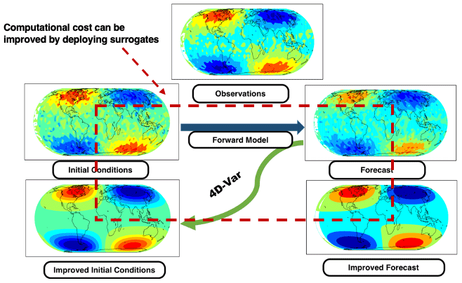
Figure 2 A schematic for 4D-Var. Performing 4D-Var improves the initial conditions of the system, which in turn improves the forecasts. However, 4D-Var requires simulating the expensive model multiple times, and this cost can be mitigated by deploying surrogates.

The prior value represents the current knowledge of the system and is frequently referred to as background in the DA community (Kalnay, 2003). The background is usually an estimate of the state x^b, along with the corresponding error covariance matrix B.

The imperfect predictions are generated by a model that approximates the physical laws that govern system evolution. The model evolution uses an initial state x₀∈ℝⁿ at initial time t₀ to obtain states x_i∈ℝⁿ at future times t_i, i.e.,

$$\begin{array}{}\text{(8)}& {\mathit{x}}_i={\mathcal{M}}_{t_{\mathrm{0}}\to t_i}\left({\mathit{x}}_{\mathrm{0}}\right),i=\mathrm{1},\mathrm{\cdots },N.\end{array}$$

The noisy data are partial observations of the true state available at discrete time instances. Specifically, measurements y_i∈ℝ^m of the true physical state x^true(t_i) are taken at discrete times t_i:

$$\begin{array}{}\text{(9)}& {\mathit{y}}_i=\mathcal{H}\left({\mathit{x}}_i\right)+{\mathit{\epsilon }}_i,{\mathit{\epsilon }}_i\sim \mathcal{N}(\mathbf{0},{\mathbf{R}}_i),i=\mathrm{1},\mathrm{\cdots },N,\end{array}$$

where the observation operator $\mathcal{H}:{\mathbb{R}}^n\to {\mathbb{R}}^m$ maps the high-dimensional model state space onto the partial (and potentially sparse) observation space. The random observation errors ε_i are assumed to be normally distributed. In general, both the model and the observation operator are nonlinear. These concepts are detailed in the following references: Daley (1993), Kalnay (2003), Sandu and Chai (2011), Sandu et al. (2005), and Carmichael et al. (2008).

Through variational methods, one may solve the DA problem by adjusting a control variable (e.g., model parameters or initial conditions) in order to minimize the discrepancy between model forecasts and observations, in a manner similar to an optimal-control framework. We next review the variational DA formulation.

3.1 Four-dimensional variational data assimilation

Strong-constraint four-dimensional variational (4D-Var) DA processes simultaneously all observations at all times $t_{\mathrm{1}},t_{\mathrm{2}},\mathrm{\dots },t_T$ within the assimilation window (see Fig. 2 for a schematic representation). The control parameters are typically given by the initial conditions x₀, which uniquely determine the state of the system at discrete instances in the future under the assumption that the model of Eq. (8) perfectly represents reality. The background state (i.e., the prior state) is the best estimate of the initial conditions ${\mathit{x}}_{\mathrm{0}}^{\mathrm{b}}$ and comes with a background error covariance matrix B₀. The 4D-Var method obtains an estimate ${\mathit{x}}_{\mathrm{0}}^{\mathrm{a}}$ of the true initial conditions by solving the following optimization problem:

$$\begin{array}{}\text{(10a)}& {\mathit{x}}_{\mathrm{0}}^{\mathrm{a}}=\underset{{\mathit{x}}_{\mathrm{0}}}{\text{arg min}}\mathcal{J}\left({\mathit{x}}_{\mathrm{0}}\right)\text{subject to}\text{Eq. (8)},\end{array}$$

$$\begin{array}{}\text{(10b)}& \begin{array}{rl}\mathcal{J}\left({\mathit{x}}_{\mathrm{0}}\right)=& {\displaystyle \frac{\mathrm{1}}{\mathrm{2}}}\Vert {\mathit{x}}_{\mathrm{0}}-{\mathit{x}}_{\mathrm{0}}^{\mathrm{b}}{\Vert }_{{\mathbf{B}}_{\mathrm{0}}^{-\mathrm{1}}}^{\mathrm{2}}+{\displaystyle \frac{\mathrm{1}}{\mathrm{2}}}\sum _{i=\mathrm{1}}^T\\ & \Vert \mathcal{H}\left({\mathit{x}}_i\right)-{\mathit{y}}_i{\Vert }_{{\mathbf{R}}_i^{-\mathrm{1}}}^{\mathrm{2}}.\end{array}\end{array}$$

The first term of the sum of Eq. (10b) captures the mismatch of the solution x₀ from the background ${\mathit{x}}_{\mathrm{0}}^{\mathrm{b}}$ at t₀. The second term measures the discrepancy between the forecast trajectory (model solutions x_i) and partial observations y_i at future times t_i in the assimilation window. The covariance matrices B₀ and R_i are usually specified a priori, and their quality influences the accuracy of the resulting solution.

3.2 Data assimilation with a surrogate model

Given a low-dimensional differentiable surrogate model, for instance, the proposed POD–LSTM, which approximates the dynamics of the full-order numerical model, the variational DA process can be accelerated dramatically. If such a surrogate model has predicted ${\widehat{\mathit{x}}}_{\mathrm{1}}$ to ${\widehat{\mathit{x}}}_T$ for a range of time steps in the reduced space (i.e., $\widehat{\mathit{x}}\approx P\mathit{x}$, $\widehat{\mathit{x}}\in {\mathbb{R}}^K$, with K≪N) and observations from the real system, y₁ to y_T are available; the objective function of the DA problem may be obtained by reconstructing the model state from the compressed representation. Here, $P:{\mathbb{R}}^N\to {\mathbb{R}}^K$ is the function that maps from physical space to reduced space. In the case of POD-based compression, P is a linear operation that projects from the physical space to the basis spanned by the truncated set of the left singular vectors of an SVD performed on snapshots from full-state model evaluation. If inversion from the truncated subspace is represented as P^†, this gives us

$$\begin{array}{}\text{(11)}& \begin{array}{rl}\mathcal{J}\left({\widehat{\mathit{x}}}_{\mathbf{0}}^{\mathbf{*}}\right)& ={\displaystyle \frac{\mathrm{1}}{\mathrm{2}}}\Vert P{\widehat{\mathit{x}}}_{\mathbf{0}}^{\mathbf{*}}-P{{\widehat{\mathit{x}}}_{\mathbf{0}}}^{\mathrm{b}}{\Vert }_{{\mathbf{B}}_{\mathrm{0}}^{-\mathrm{1}}}^{\mathrm{2}}\\ & +{\displaystyle \frac{\mathrm{1}}{\mathrm{2}}}\sum _{i=\mathrm{1}}^T\Vert \mathcal{H}\left(P^{†}{\widehat{\mathit{x}}}_i\right)-{\mathit{y}}_i{\Vert }_{{\mathbf{R}}_i^{-\mathrm{1}}}^{\mathrm{2}}.\end{array}\end{array}$$

Note that ${\widehat{\mathit{x}}}_i$, which is an approximation to the compressed state at time t_i, is evaluated using the surrogate model – that is, by propagating ${\widehat{\mathit{x}}}_{\mathbf{0}}^{\mathbf{*}}$ using the surrogate model (LSTM in this case). The operation $P^{†}{\widehat{\mathit{x}}}_i$ represents reconstruction of the full-order state from its compressed representation. Given a projection operation P with an effective compression ratio (obtained from our dimensionality reduction technique), Eq. (10b) becomes a cost function as shown in Eq. (11) expressed in K dimensions which is amenable to rapid updates of the initial conditions. Moreover, gradients of this objective function with respect to the initial conditions are trivially computable because of the use of automatic differentiation of our LSTM neural network. The overall approach is as follows:

• For each forecast window, collect random observations from the true state.

• Perform an optimization of Eq. (11) by perturbing the inputs to the LSTM neural network. This input is the projected version of the initial-condition state.

• If optimization has converged, perform one forecast with the optimized initial condition. This is the DA-improved forecast.

The optimization methodology used in this article is the sequential least-squares programming approach (Nocedal and Wright, 2006) implemented in SciPy. The neural architecture was deployed using TensorFlow 2.4. Our overall implementation is in Python.

4 Results

We describe the dataset used in our experiments and then present our experimental results.

4.1 Dataset

The data used in this study are a subset of 20 years of output from the regional climate model Weather Research and Forecasting (WRF) version 3.3.1, prepared with methods and configurations described by Wang and Kotamarthi (2014). WRF is a fully compressible and nonhydrostatic regional numerical weather prediction system with proven suitability for a broad range of applications. The WRF simulations used by this study are driven by reanalysis data of NCEP Reanalysis 2 (NCEP-R2) for the period 1984–2003. The NCEP-R2 dataset assimilates many of the observational datasets available to build dynamically consistent gridded fields that are typically used for initialization and the boundary condition setting for forecasting models. The WRF simulation domain is centered at 52.24^∘ N, 105.5^∘ W and has dimensions of 600×516 horizontal grid points in the west–east and south–north directions with a grid spacing of 12 km, covering most of North America. A spectral-nudging technique is applied for zonal and meridional winds, temperature, and geopotential height at each vertical level above 850 hPa (e.g., around 1.5 km).

We use geopotential height of the 500 hPa pressure surface (Z500 hereafter) from WRF output to demonstrate the approach developed in this study. The geopotential height represents the height of pressure surface above sea level; for Z500, it is around 5.5 km, and it is often referred to as a steering level. The weather systems beneath, near to Earth's surface, roughly move in the same direction as the winds at the 500 hPa level. This is also the level where one can look for vertical motions. Z500 has been used as one of the standard fields for weather forecasting because it does not have very strong local gradients (in contrast to fields such as humidity or precipitation) and does not depend on local conditions such as topography, yet most of the important global flow patterns – such as midlatitude jets and a gradient between poles and Equator – are visible in Z500. Low Z500 values indicate troughs and cyclones (e.g., favorable to precipitation) in the middle troposphere, while high Z500 values indicate ridges and anticyclones.

We retrieve the Z500 data from the WRF output at a grid spacing of 12 km and at 3 h intervals with 515×599 grid cells in the south–north and west–east directions, respectively. We then calculate per-grid-point daily averages to obtain one data value per grid point per day. Spatially, we coarsen the data by five strides (uniform subsampling), which still maintains the spatial patterns of Z500 but reduces the data size significantly. Each daily Z500 snapshot therefore comprises 102×119 grid points of 60×60 km. We have 3287 such daily snapshots for the period 1 January 1984 to 31 December 1991. Despite the coarsening of the original 12 km data, the typical eastward-propagating waves are clearly visible in the Northern Hemisphere. Such waves are also observed in the real atmosphere and are one of the main features of midlatitude weather variability on timescales of several days.

We use the first 6 years of the daily averaged Z500 WRF data (1984–1989) for surrogate training and optimization. Of those data, we select 70 % at random as training data, for use in training the supervised ML formulation, and keep the remaining 30 % as validation data, for use in tuning the neural-architecture hyperparameters and to control overfitting (a situation in which the trained network predicts well on the training data but not on the test data). We also construct a set of test data consisting of 1 year of records (1991) for prediction and evaluation. We skip 1990 so as to ensure that there is no overlap in input windows.

We assume that the observation errors are uncorrelated. This is realistic, as the sensors can be assumed to be independent. However, this assumption might not hold in the case of certain instruments such as lidar, where the errors can be spatially and temporally correlated. We will explore the use of correlated observation errors in our future research. We assume the standard deviation of the observation errors to be approximately 1.5 % of the mean value. In our future studies, in addition to using a realistic observation error covariance matrix, we will also pursue using a flow-dependent background error covariance matrix, as described in Buehner (2005).

4.2 Experiments

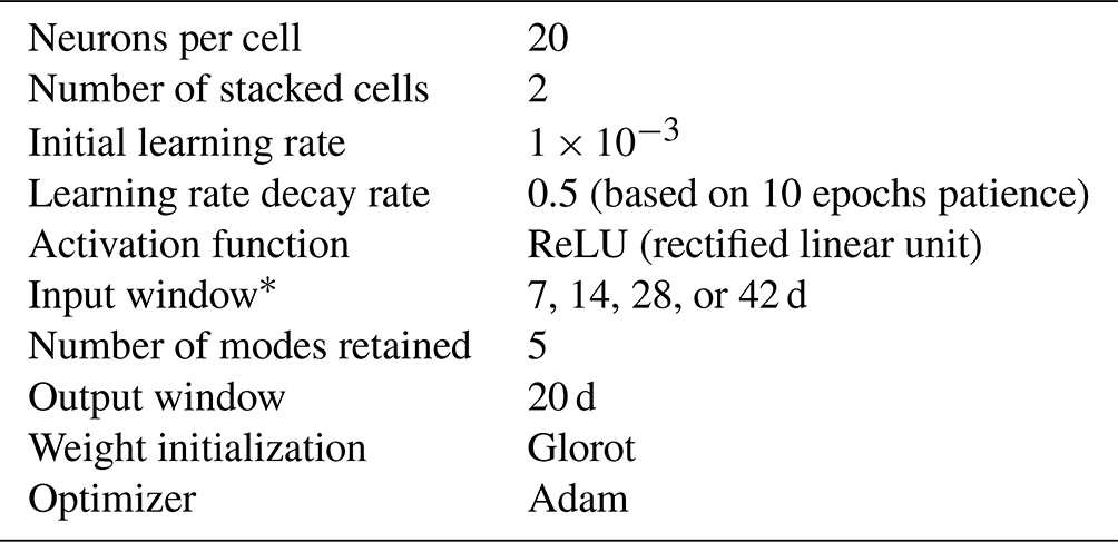
We conduct a number of experiments to evaluate the performance of our emulator-assisted DA approach. In the first one, we perform a grid-based search in which we vary both the number of POD modes (5, 10, and 15) and the size of the input window (7, 14, 28, or 42 d of lead-time information) to identify the optimal combination for forecasting. Other hyperparameters such as learning rate, learning rate scheduler, number of LSTM cells, and number of neurons are determined by a combination of experience in previous modeling tasks, considerations of computational efficiency, and limited manual tuning. We set the output forecast window to 20 d to represent a difficult forecast task for the emulator.

We give the complete set of hyperparameters for our problem in Table 1. We found that the lowest validation errors were achieved when just five modes were retained, a result that matches earlier studies (Lario et al., 2021), where increasing the number of modes is seen to cause difficulties in long-term forecasting (for example, for more than 2 weeks). The training and validation data are used in this phase of our experimentation to identify the best model for performing accelerated DA. We train the neural network architecture by penalizing the loss function on the training data while using the validation data to enforce an early stopping criterion (i.e., prevent overfitting). Once the different models have been trained, the best model is determined by studying the validation losses of all the different architectures. This model is then used for testing on unseen data and for DA. For a further sensitivity analysis of this model, we trained four other models with varying input window sizes (7, 28, 35, and 42) and different random seeds, with other hyperparameters fixed, and utilized them for obtaining ensemble test results. We trained and validated architectures using multiple hyperparameters in parallel by using Ray (Moritz et al., 2018), a TCP/IP-based (Transmission Control Protocol–Internet Protocol) parallelization protocol, on Nvidia A100 graphics processing units (GPUs) of the Argonne Leadership Computing Facility's Theta supercomputer.

Table 1 LSTM hyperparameters used when training the low-dimensional surrogate. The quantity with an asterisk is varied, in addition to random seeds, for sensitivity analyses of the surrogate model where, in addition to the best chosen model here, several other models are trained with different weight initializations and input window sizes.

Our first set of assessments test the POD–LSTM emulator without any DA. We show in Fig. 3 (in the left column) how emulator predictions for day 15 (for all forecasts in the test dataset) compare to climatology. Climatology, here, refers to the average forecast on a specific forecast day based on averaged training data. For instance, if geopotential height is to be forecast on 7 December 1991, the climatology prediction would be the average of 7 December geopotential height values for 1984–1989. The metrics we use for comparison first include the cosine similarity improvement as shown in Fig. 3a. Here, the cosine similarity (which captures the alignment between prediction and truth) obtained from climatology is subtracted from that obtained from the emulator forecast. Thus, in this case, negative (blue) regions are where climatology captures the temporal trend of the forecast better than our emulator. In Fig. 3c, we subtract the mean absolute error (MAE) of the emulator predictions from that of climatology. Here, the blue regions are where climatology is more accurate on average than the emulator. Figure 3e merely shows the MAE for the emulator. From this analysis, it is clear that for large regions in the data domain (particularly in the north), the emulator performs quite poorly.

We next assess results from applying DA through random observations at 5000 locations of the domain to see if results obtained with the emulator can be improved. Here, sparse observations at each time step of the output window are used within the optimization statement introduced in Eq. (11) to update the initial conditions (i.e., the input window). We emphasize that the observations are obtained randomly from the true state of the system during forecasts, which corresponds to the test data introduced previously.

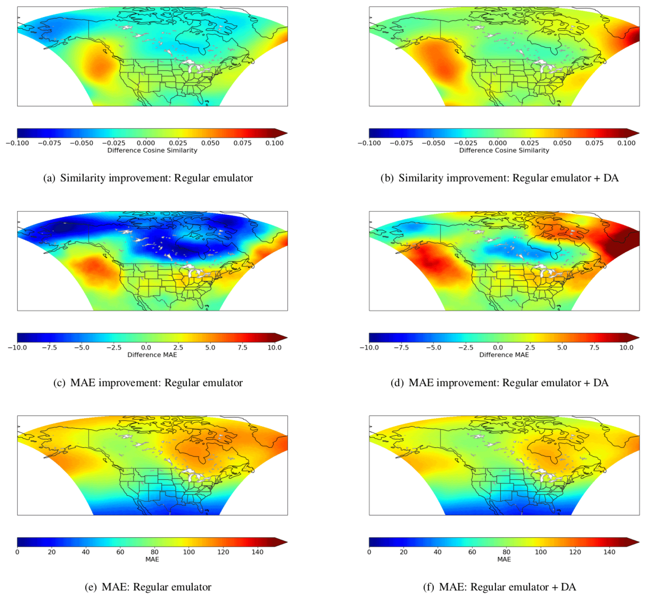
Figure 3 Improvements over climatology for the regular emulator (a, c, e) and DA-corrected emulator (b, d, f) when using the best set of hyperparameters as determined on validation data. Here cosine similarity captures an agreement in the trend between forecast and truth, and MAE refers to the mean absolute error between the same. These contours are averaged over all forecasts.

Figure 4 Geopotential height forecast MAEs for 20 d, relative to the true test data, for seven National Climate Assessment subregions of continental North America (Reidmiller et al., 2018), from both a regular ML emulator and the same emulator corrected by variational DA. Confidence intervals, for five separately trained emulators, encapsulate the effects of perturbations to the random seed and the input window. DA-based correction gives both lower MAEs and narrower confidence intervals.

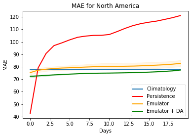
Figure 5 Geopotential height forecast MAEs for 20 d for continental North America, relative to the true test data. Results describe performance of a regular ML emulator and the same emulator corrected by variational data assimilation. Here we also show the results of persistence, which is outperformed in the long-term prediction regime as expected.

The results for using DA, in the right column of Fig. 3, show that the use of sensor information aids the forecast immensely, improving performance in all metrics significantly by virtue of DA. In particular, the proposed augmentation (i.e., the use of DA during forecasts) reduces forecast errors considerably in regions where the sole use of the emulator was not competitive. We provide MAE assessments for our 20 d output averaged over the testing data range in Fig. 4, where we compare the raw emulator outputs, climatology, persistence, and the DA-corrected outputs. We also provide confidence intervals for the regular (i.e., without DA) and DA-corrected emulators, where the five different emulators are trained with different random seeds and input window durations to assess the sensitivity to the initialization of the training as well as the automatic-differentiation-based optimization. The results indicate that the DA-corrected emulation is the most accurate and consistent forecast technique.

We also provide in Fig. 5 a comparison with another benchmark, persistence, which uses the state of the last day in the input window as the forecast for each day of the output window. Persistence is seen to be more accurate for short lead times but is outperformed by both climatology and data-driven methods for longer forecast durations.

Our choice of 20 d for the forecast window was motivated by the results of Rasp et al. (2020) and Rasp and Thuerey (2021), who performed analyses for 5 d forecasts. Our study increased the forecast window to 4 times the original assessments for geopotential height to demonstrate the possibility of improved forecasting of any emulator using automatic-differentiation-enabled variational DA. In many subregions of the computational domain, the use of DA with the emulator is also seen to improve on climatology predictions – even at large lead times (20 d out), where classical data-driven and numerical forecast models are typically less accurate than climatology.

Our method also delivers large computational gains. A 1-year forecast with the emulator-assisted DA performed each day takes approximately 1 h on a single processor core without any accelerator hardware. In contrast, the original PDE-based simulation required 21 600 core hours for a 1-year forecast with a 515×599 grid. (A coarse-grained forecast for 1 year on the 103×120 grid used here takes 172 core hours, but the resulting flow field does not adequately reproduce the fidelity of the 515×599 grid.) One can observe significant speedup (∼ 10⁴ times) for the emulation of the geopotential height, even without factoring the cost of an additional variational DA step. Furthermore, the solution to the 4D-Var problem, which yields an improved initial condition, requires on the order of 100 model runs, where each model run can be several orders of magnitude more expensive than our emulator.

5 Conclusions

We have described how a differentiable reduced-order surrogate geophysical forecasting model may be integrated into an outer-loop optimization technique whereby real-time observations of the true solution are used to improve the forecast of the surrogate. We use such observations to improve the initial condition of the surrogate model such that an optimization statement given by the classical four-dimensional variational DA objective function is minimized. The use of the reduced-order surrogate converts a high-dimensional optimization to one that is given by the dimensionality of the compressed representation and the duration of the input window for forecasting. Our optimization is thus performed rapidly, given sparse and random observations from the true flow field, without any access to high-performance computing resources. Computational costs are reduced by 4 orders of magnitude, by virtue of the surrogate-assisted forecasting and variational DA, when compared to a classical equation-based forecasting of the dynamics. We assess our model on a real-world forecasting task for geopotential height in the continental US and obtain competitive results with respect to climatology and persistence baselines for mean absolute error and cosine similarity.