Evaluation of a quasi-steady-state approximation of the cloud droplet growth equation (QDGE) scheme for aerosol activation in global models using multiple aircraft data over both continental and marine environments

This research introduces a numerically efficient aerosol activation scheme and evaluates it by using stratus and stratocumulus cloud data sampled during multiple aircraft campaigns in Canada, Chile, Brazil, and China. The scheme employs a quasi-steady-state approximation of the cloud droplet growth equation (QDGE) to efficiently simulate aerosol activation, the vertical profile of supersaturation, and the activated cloud droplet number concentration (CDNC) near the cloud base. The calculated maximum supersaturation values using the QDGE scheme were compared with multiple parcel model simulations under various aerosol and environmental conditions. The differences are all below 0.18 %, indicating good performance and accuracy of the QDGE scheme. We evaluated the QDGE scheme by specifying observed environmental thermodynamic variables and aerosol information from 31 cloud cases as input and comparing the simulated CDNC with cloud observations. The average of mean relative error ($\stackrel{\mathrm{‾}}{\mathrm{MRE}}$) of the simulated CDNC for cloud cases in each campaign ranges from 17.30 % in Brazil to 25.90 % in China, indicating that the QDGE scheme successfully reproduces observed variations in CDNC over a wide range of different meteorological conditions and aerosol regimes. Additionally, we carried out an error analysis by calculating the maximum information coefficient (MIC) between the MRE and input variables for the individual campaigns and all cloud cases. MIC values were then sorted by aerosol properties, pollution level, environmental humidity, and dynamic condition according to their relative importance to MRE. Based on the error analysis, we found that the magnitude of MRE is more relevant to the specification of input aerosol pollution level in marine regions and aerosol hygroscopicity in continental regions than to other variables in the simulation.

1 Introduction

Aerosols play an important role in determining the radiation balance of the Earth–atmosphere system by scattering and absorbing shortwave radiation and altering the cloud reflectivity and lifetime (Twomey, 1974, 1977; Ghan, 2013; Forster et al., 2016; Ramaswamy et al., 2019; Wang et al., 2020). Currently, aerosol–cloud interactions are one of the largest sources of climate modeling uncertainty (IPCC AR6, Forster et al., 2021).

Aerosol–cloud interactions are largely driven by the activation of aerosols to form cloud droplets. The addition of activated aerosol to existing clouds can directly change the concentration and size of cloud droplets and thereby affect the microphysical properties and radiative forcing of the clouds. Aerosol activation is controlled by rapid and non-linear aerosol and cloud microphysical processes (Meskhidze et al., 2005), which have not been explicitly resolved in climate models yet (Fountoukis et al., 2007; Kang et al., 2015). Nenes et al. (2001) pointed out that the cloud droplet activation process is subject to kinetic limitations, including inertial, evaporation, and deactivation mechanisms, which further adds to the complexity of the aerosol activation.

Early parameterizations of aerosol activation in climate models were based on observations and derived through parameter fitting, using the aerosol number or mass concentration or other cloud condensation nuclei (CCN) proxies (e.g., sulfate mass) to empirically determine the activated cloud droplet number concentration (CDNC) (Jones et al., 1994; Boucher and Lohmann, 1995; Jones and Slingo, 1996; Lohmann, 1997; Kiehl et al., 2000; Menon et al., 2002). Although these parameterizations have the advantages of convenience and low computational burden (Fountoukis et al., 2007), substantial uncertainties result from limited spatiotemporal representativeness and unresolved variations in aerosol properties (Meskhidze et al., 2005). In the two recent decades, physically based parameterization schemes of aerosol activation have emerged (Abdul-Razzak and Ghan, 2000; Cohard et al., 2000; Fountoukis and Nenes, 2005; Ming et al., 2006; Kivekäs et al., 2008; Khvorostyanov and Curry, 2009; Shipway and Abel, 2010; Zhang et al., 2015). These schemes are based on the Köhler theory and are used in climate models to parameterize aerosol activation near the cloud base. As Köhler theory fundamentally describes the process by which water vapor condenses and forms liquid cloud droplets, it can be applied to a wide range of atmospheric conditions and aerosol pollution levels. However, considerable approximations of the Köhler theory are employed for application in climate models, which leads to potential biases in comparison with results from more rigorous and accurate simulations of cloud droplet growth with adiabatic parcel models (e.g., Ghan et al., 2011). The ongoing increase in computing power (Herrington and Reed, 2020) reduces the need for cost-saving approximations in climate models. In the following, we will introduce a quasi-steady-state approximation of the cloud droplet growth equation (QDGE) that provides an efficient alternative to parameterizations of activated CDNC in climate models.

Parameterization schemes of aerosol activation have often been evaluated using adiabatic parcel model simulations. These models explicitly solve aerosol activation and droplet growth processes by mimicking vertical uplifting of an air parcel containing a specified number of aerosol particles, predicting changes in temperature, humidity or supersaturation, activation of aerosols, and droplet growth from the cloud base upward. When utilizing identically specified aerosols, the results of a parcel model can be used as a benchmark to evaluate parameterizations. This approach has been used extensively to evaluate activation schemes (Table 1). However, a less commonly used approach is to evaluate parameterizations by conducting a “closure experiment”, that is, to carry out a parameterized calculation by specifying observed aerosol concentrations and environmental thermodynamic conditions and then compare the calculated and observed CDNC (e.g., Snider and Brenguier, 2000; Guibert et al., 2003; Fountoukis and Nenes, 2005; Kivekäs et al., 2008). Though some parameterizations have been evaluated based on comparisons of simulated and observed CDNC from aircraft campaigns, mostly regional datasets have been used for very specific meteorological conditions and pollution levels. It is essential to select a wide range of cloud data for different atmospheric conditions and pollution levels to arrive at meaningful conclusions for global climate model (GCM) simulations.

In this study, we introduce the QDGE scheme and evaluate it by using cloud data from multiple aircraft campaigns in four different regions over the world, covering marine and continental conditions. This paper is organized as follows. The next section describes the QDGE scheme, and Sect. 3 summarizes the data and methods used for the closure experiment. Section 4 illustrates the results of the closure experiment and analyzes the sources of simulation errors, followed by conclusions and discussion in Sect. 5.

Table 1 A summary of activation parameterizations and the evaluation methods in previous studies.

2 QDGE scheme

2.1 Scheme description

Aerosol particles suspended in an air parcel grow into cloud droplets by condensation of water vapor if supersaturation with respect to water exceeds a critical value. In stratus and convective clouds, aerosol activation is particularly efficient in the vicinity of the cloud base, where supersaturation typically reaches its local maximum. Although observations provide evidence that aerosol activation is not limited to the region near the cloud base, this is omitted in the aerosol activation scheme described here, similar to most models and parameterizations.

In order to determine the portion of the aerosols that activate and form cloud droplets, a numerical solution of the condensational droplet growth equation (e.g., Seinfeld and Pandis, 2016) is employed to simulate the growth of an ensemble of aerosol particles near the cloud base. The number of activated cloud droplets above the cloud base is simulated by solving a series of equations that describe a vertically ascending air parcel containing aerosols. The vertical velocity of the air parcel, w_c (in m s⁻¹), is either specified or parameterized, as described in Sect. 3.2.3.

The change in wet aerosol particle radius, R_pw, by condensation of water vapor as a function of the environmental supersaturation (S, e.g., Emanuel, 1994) in the scheme is given by

$$\begin{array}{}\text{(1)}& R_{\mathrm{pw}}{\displaystyle \frac{\mathrm{d}{R}_{\mathrm{pw}}}{\mathrm{d}t}}={\displaystyle \frac{S-S_{\mathrm{p}}}{C}},\end{array}$$

where S_p is the equilibrium supersaturation over the surface of the particle, which is obtained from κ-Köhler theory (Petters and Kreidenweis, 2007):

$$\begin{array}{}\text{(2)}& S_{\mathrm{p}}={\displaystyle \frac{A}{R_{\mathrm{pw}}}}-{\displaystyle \frac{B}{R_{\mathrm{pw}}^{\mathrm{3}}}},\end{array}$$

where the parameters A, B, and C account for thermodynamic conditions in the cloud and physiochemical properties of the aerosol particles and droplets (Appendix A).

As described below, the QDGE scheme solves Eqs. (1) and (2) in combination with energy and moisture budgets to calculate changes in S driven by thermodynamic processes. For instance, the thermodynamic equations underlying the QDGE scheme can be used to obtain the temporal evolution of S in the air during adiabatic ascent near cloud base (Ghan et al., 2011):

$$\begin{array}{}\text{(3)}& {\displaystyle \frac{\mathrm{d}S}{\mathrm{d}t}}=D{w}_{\mathrm{c}}-E{\displaystyle \frac{\mathrm{d}{q}_{\mathrm{w}}}{\mathrm{d}t}},\end{array}$$

where the parameters D and E are weak functions of temperature and pressure, and q_w is the liquid water mixing ratio, which is related to the activated particle size distribution (Appendix A).

Theoretically, each growing aerosol particle will compete with others for the water vapor in the environment, and the particle size increases according to Eq. (1) and affects the environmental supersaturation through Eq. (3). Equations (1)–(3) are coupled in a complex manner; thus, they hardly have an analytical solution. For example, Eq. (3) indicates that the balance between the enhancement of S due to the air parcel uplifting, and the reduction of S due to the condensation growth of activated particles, leads to a highly non-linear variation of S with time in the ascending parcel of cloudy air. The condensation growth is non-linearly related to the environmental conditions and aerosol properties (Eqs. 1–2). Therefore, a time step much shorter than 1 s is typically required to numerically solve these equations, which implies computational expenses that would prohibit applications in climate models (Khain et al., 2015). For instance, adiabatic ascending parcel models (e.g., Chen et al., 2016; Peng et al., 2005) to numerically solve Eqs. (1)–(3) require a very high time resolution, typically with a time step of 10⁻³ to 10⁻⁴ s.

In large-scale stratus clouds, the maximum supersaturation (usually less than 0.2 %) occurs about 100 m above the cloud base; that is, the rate of S change is 0.002 % m⁻¹ or so. A similar conclusion can be derived from the change of supersaturation and temperature (combined with a lapse rate of atmospheric temperature; Pandis et al., 1990). Therefore, it is reasonable to assume a scale of several seconds (or meters) at which the supersaturation is approximately constant in the air parcel. Consequently, we use the QDGE, which assumes that the local S is approximately constant. Equation (1) can then be conveniently expressed as follows:

$$\begin{array}{}\text{(4)}& {\displaystyle \frac{\mathrm{d}x}{\mathrm{d}u}}=\mathit{\delta }-a\left({\displaystyle \frac{b}{x^{\mathrm{1}/\mathrm{2}}}}-{\displaystyle \frac{\mathrm{1}}{x^{\mathrm{3}/\mathrm{2}}}}\right),\end{array}$$

for the time period from t to t+Δt_s (Δt_s is a sub-time step, roughly several tens of seconds), with variable substitutions for particle size, $x=R_{\mathrm{pw}}^{\mathrm{2}}/\mathrm{2}$, and for time, $u=t\mathrm{|}S\mathrm{|}/C$, and parameters that are given by

$$\begin{array}{}\text{(5)}& \mathit{\delta }=\left\{\begin{array}{lll}-\mathrm{1},& \mathrm{if}& S<\mathrm{0},\\ \mathrm{1},& \mathrm{if}& S\ge \mathrm{0},\end{array}\right.,\end{array}$$

$$\begin{array}{}\text{(6)}& {\displaystyle }a={\displaystyle \frac{B}{{\mathrm{2}}^{\mathrm{3}/\mathrm{2}}\left|S\right|}},\text{(7)}& {\displaystyle }b={\displaystyle \frac{\mathrm{2}A}{B}}.\end{array}$$

In the QDGE scheme, pre-calculated solutions of Eq. (4) are used, which are provided in the form of look-up tables (LUTs) for different values of a, b, and δ in the model to calculate R_pw. The S-dependent parameters a and δ, and u are determined through an iterative procedure for each time step and vertical level near cloud base, as described in the following.

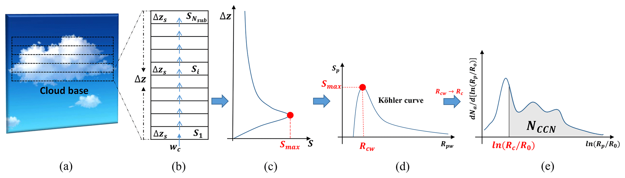
The major steps of the QDGE scheme are shown in Fig. 1. A vertical grid with N_sub sublevels (grid spacing $\mathrm{\Delta }{z}_{\mathrm{s}}=\mathrm{\Delta }z/N_{\mathrm{sub}}$) is employed in the QDGE scheme, where Δz is the grid spacing in the atmospheric host model, near cloud base (Fig. 1a–b). Calculations are only performed for the first host model grid layer above the cloud base, with typical values Δz_s≈1–10 m. The local approximation with constant S applies in each sublevel Δz_s, and a vertical profile of S is eventually obtained within the host model grid Δz (Fig. 1c). The iterative calculation to obtain S at each sublevel is described below.

Figure 1 A schematic diagram to show the major steps of the QDGE scheme.

In each sublevel Δz_s, supersaturation (i.e., S_i in Fig. 1b, where $i=\mathrm{1},\mathrm{\dots }{N}_{\mathrm{sub}}$) and the S-dependent parameters in Eq. (4) are obtained through an iterative calculation, which explicitly requires the conservation of mass and energy. The flow chart of the iterative calculation is shown in Fig. 2.

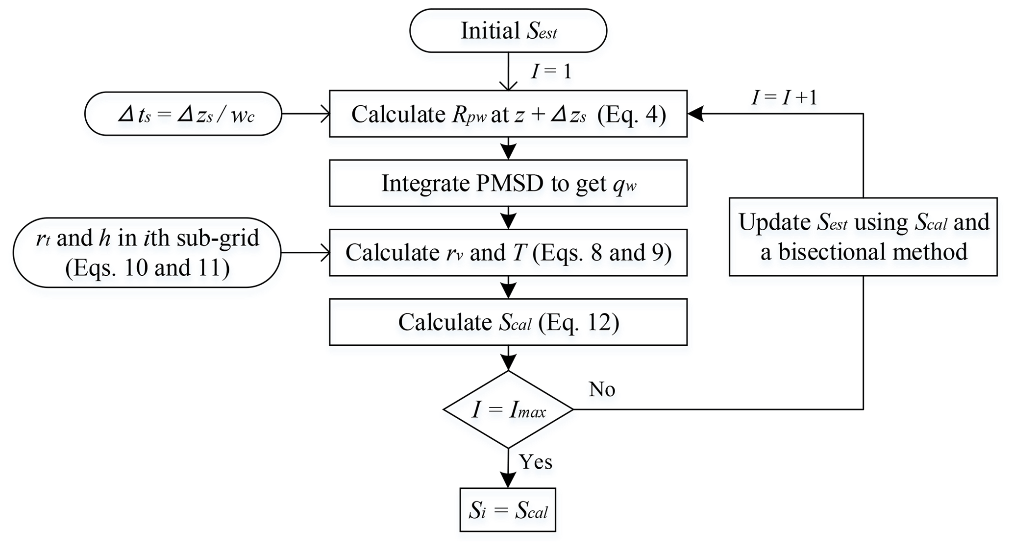
Figure 2 The flow chart of the iterative calculation for the subgrid supersaturation S_i. I is the number of iterations. PMSD is the particle mass-size distribution. Total water mass mixing ratio, r_t, and liquid water static energy, h, are conserved.

At the beginning of an iteration, an initial value of supersaturation (S_est) is specified and Eq. (4) is integrated over the sub-time step $\mathrm{\Delta }{t}_{\mathrm{s}}=\mathrm{\Delta }{z}_{\mathrm{s}}/w_{\mathrm{c}}$ to obtain a first estimate of the particle wet size R_pw at the sublevel z+Δz_s. Next, an integration over the particle mass-size distribution (PMSD) yields a first estimate of the liquid water mixing ratio q_w at z+Δz_s (Fig. 2).

The subsequent calculations are based on the total water mass mixing ratio, r_t, and liquid water static energy, h, defined as

$$\begin{array}{}\text{(8)}& {\displaystyle }{r}_{\mathrm{t}}=r_{\mathrm{v}}+q_{\mathrm{w}},\text{(9)}& {\displaystyle }h=gz+c_{\mathrm{p}}T-L_{\mathrm{v}}{q}_{\mathrm{w}},\end{array}$$

where, r_v is the water vapor mass mixing ratio, T is the temperature, g is the gravitational constant, and c_p is the heat capacity at a constant pressure of dry air. The total water mass mixing ratio and liquid water static energy at the lower and upper boundaries of the current host model grid (with the superscripts L and U, respectively) are first calculated using Eqs. (8) and (9). Then, the total water mass mixing ratio ($r_{\mathrm{t}}^i$) and liquid water static energy (hⁱ) in the ith sublevel are obtained by linear interpolation, given by

$$\begin{array}{}\text{(10)}& {\displaystyle }{r}_{\mathrm{t}}^i={\displaystyle \frac{N_{\mathrm{sub}}-i+\mathrm{1}}{N_{\mathrm{sub}}}}{r}_{\mathrm{t}}^{\mathrm{L}}+{\displaystyle \frac{i-\mathrm{1}}{N_{\mathrm{sub}}}}{r}_{\mathrm{t}}^{\mathrm{U}},\text{(11)}& {\displaystyle }{h}^i={\displaystyle \frac{N_{\mathrm{sub}}-i+\mathrm{1}}{N_{\mathrm{sub}}}}{h}^{\mathrm{L}}+{\displaystyle \frac{i-\mathrm{1}}{N_{\mathrm{sub}}}}{h}^{\mathrm{U}}.\end{array}$$

Knowing $r_{\mathrm{t}}^i$ and hⁱ, r_v and T in the ith sublevel can be derived from Eqs. (8) and (9) using the estimated q_w. Subsequently, the supersaturation S is calculated, based on the standard definition of the water vapor saturation ratio,

$$\begin{array}{}\text{(12)}& S+\mathrm{1}={\displaystyle \frac{r_{\mathrm{v}}}{r_{\ast }}}\left({\displaystyle \frac{\mathrm{1}+r_{\ast }/\mathit{\epsilon }}{\mathrm{1}+r_{\mathrm{v}/\mathit{\epsilon }}}}\right),\end{array}$$

where ε≡0.622, and r_∗ is the saturation water vapor mass mixing ratio in the air parcel, which depends on T.

The calculated supersaturation (S_cal) after each iteration is compared to the initial estimate S_est. An improved estimate of S is determined using a bisectional method that minimizes the difference between different available estimates of S through iteration, as shown in Fig. 2. The method enables quick convergence to a good-enough estimated value of S, which solves Eq. (4) and satisfies all necessary constraints according to Eqs. (8), (9), and (12). Here, the maximum number of iterations (I_max) was set to 4 for the model applications discussed below. The iterations are repeated in each sublevel to calculate S_i until the vertical profile of supersaturation is available at all N_sub levels (Fig. 1b).

The maximum value of the simulated vertical supersaturation profile, S_max, is used to diagnose the critical particle size, R_cw, based on Eq. (2) (Fig. 1c–d). Correspondingly, the dry particle size (R_c) for activation can be determined according to R_cw and the aerosol size distribution. All particles with a radius larger than R_cw are taken as the activated particles to become cloud condensation nuclei. Consequently, the cloud condensation nuclei number concentration (N_CCN) is obtained by integrating the activated aerosol size distribution accordingly (Fig. 1e). Above cloud base, a uniform number of the activated particles is assumed, equal to the value calculated at cloud base, in good agreement with observations and detailed simulations using cloud resolving models (Gerber et al., 2008; Slawinska et al., 2012; Jarecka et al., 2013).

In each grid of the host model, the dry aerosol number-size distribution is represented as particle numbers at regular size intervals, $\mathrm{\Delta }\mathit{\chi }=\mathrm{1}/p\mathrm{\Delta }\mathit{\phi }$, where p is the number of size bins. Δφ is the particle size range covering both Aitken and accumulation modes, expressed in terms of a dimensionless particle size parameter $\mathit{\phi }=\ln (R_{\mathrm{p}}/R_{\mathrm{0}})$, with $R_{\mathrm{0}}={\mathrm{10}}^{-\mathrm{6}}$ m. In this study, we set p to 6, meaning that six discrete aerosol particle size bins are used. The continuous aerosol size distribution (such as Fig. 1e) can be obtained from linear interpolation using the particle numbers in six discrete size bins.

Currently, only adiabatic processes are considered in each sublevel, and therefore total water mass mixing ratio (r_t) and liquid water static energy (h) are conserved as the parcel ascends from z to z+Δz_s. However, energy and moisture profiles in clouds may be affected by entrainment processes. Therefore, we additionally consider the impact of entrainment on r_t and h above the cloud base by using

$$\begin{array}{}\text{(13)}& {\displaystyle }{r}_{\mathrm{t}}^{\mathrm{U}e}=r_{\mathrm{t}}^{\mathrm{L}}+(r_{\mathrm{t}}^{\mathrm{U}}-r_{\mathrm{t}}^{\mathrm{L}})\exp (-e\mathrm{\Delta }z),\text{(14)}& {\displaystyle }{h}^{\mathrm{U}e}=h^{\mathrm{L}}+(h^{\mathrm{U}}-h^{\mathrm{L}})\exp (-e\mathrm{\Delta }z),\end{array}$$

where $r_{\mathrm{t}}^{\mathrm{U}e}$ and h^Ue are the total water mass mixing ratio and liquid water static energy considering the entrainment of air, with a specified entrainment rate given by e, respectively. These can be used to replace $r_{\mathrm{t}}^{\mathrm{U}}$ and h^U in Eqs. (10) and (11) when entrainment needs to be considered.

Note that Eq. (3) can only be used for an adiabatic process and does not work if there is entrainment or radiative cooling of the air, e.g., the formation of cloud droplets in radiation fog. In contrast, the QDGE scheme is much more general, as outlined above. The QDGE scheme can be easily modified for simulations of entrainment and radiation fog if required.

2.2 Comparison with a parcel model

In this subsection, we examine the performance of the QDGE scheme by comparing it with parcel model results by conducting a series of experiments as described in Ghan et al. (2011). The parcel model can numerically solve the droplet growth equation in a most accurate way by representing aerosol size distributions with finely discretizing bins and utilizing a very short time step to trace the supersaturation variation with time/height (Ghan et al., 2011).

For the comparisons, we assume a trimodal lognormal size distribution (Whitby, 1978) of ammonium sulfate aerosol, consistent with the experimental setup in Ghan et al. (2011) (Table B1). The environmental conditions in the simulations cover a wide range of w_c values (0.1–10 m s⁻¹) and four different aerosol regimes (marine, clean continental, background, and urban). When conducting QDGE simulations, we set the number of sublevels (N_sub), the maximal number of iterations (I_max), and the number of size bins (p) as 60, 4, and 6, respectively, which are the same as those in the following closure experiment (Sect. 4.1). Comparison between the results from the simulations are shown in Fig. 3, in which the parcel model results are identical to those in Ghan et al. (2011). In general, the QDGE scheme performs well with lower w_c but overestimates the S_max when w_c is larger than 2 m s⁻¹. The differences in S_max between parcel model and the QDGE scheme in all experiments are within 0.18 % (with an average of 0.05 %), much lower than the differences between parcel model and four state-of-the-art activation schemes (within approximately ±1.5 %) in Ghan et al. (2011). This indicates that the QDGE scheme achieves a high accuracy in simulating the processes of activation and condensation growth of cloud droplets under the specified conditions.

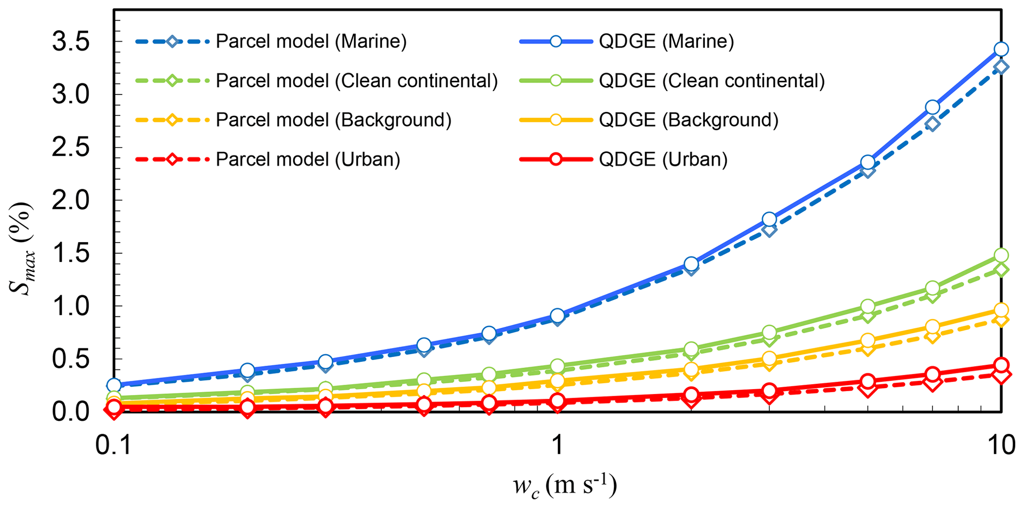
Figure 3 Comparison between the calculated maximum supersaturation (S_max) from the QDGE scheme (solid line) and the parcel model (dashed line, Ghan et al., 2011).

In contrast to the QDGE scheme, the four activation schemes considered by Ghan et al. (2011) are based on parameterized and simplifying assumptions about the physical processes involved in the formation of clouds droplets, using the vertical grid of the host model. Therefore, the QDGE scheme can be used for a broader range of environmental and aerosol conditions than these schemes, in general. Although the QDGE scheme mimics the parcel model well, it is also numerically efficient. Typically, a parcel model simulation will take several minutes, while the QDGE scheme only consumes 0.1 s for the same case using a single core on Intel Xeon E5-2660 v2.

One more advantage of the QDGE scheme is the potential scale adaptivity for different vertical grids. The accuracy of the simulated supersaturation profile increases with the specified number of sublevels (N_sub) and the number of iterations (I_max). Therefore, as the supercomputer capabilities for climate model simulations are improved, the QDGE scheme will provide a more accurate solution for the activation process and easily adapts to the accuracy requirement for high-resolution GCMs in the future.

An earlier version of the QDGE scheme has been successfully used for simulations with the fifth generation of the Canadian atmospheric global climate model (CanAM5). It is currently being tested in additional models.

3 Data and methods

3.1 Campaign description

The worldwide cloud data used for the evaluation were sampled from four aircraft campaigns. The locations and instrument information of the four campaigns are shown in Fig. 4 and Table 2. The Canada (CAN) campaign provided marine stratus cloud data observed during the Radiation, Aerosol and Cloud Experiment (RACE) in the fall of 1995 off the coast of Nova Scotia, Canada (Peng et al., 2002). The Chile (CL) campaign provided marine stratocumulus cloud data observed during the VAMOS Ocean-Cloud-Atmosphere-Land Study Regional Experiment (VOCALS-REx), for near-climatological atmospheric conditions off northern Chile and southern Peru (Wood et al., 2011). The Brazil (AMA) campaign provided continental stratus clouds data observed in Manaus, Brazil, during the Green Ocean Amazon (GoAmazon2014/5) Experiment (Martin et al., 2016). The China (CN) campaign provided polluted continental stratus cloud data sampled in Beijing, China, by the Beijing Weather Modification Office (Liu et al., 2020). These worldwide datasets comprise continental (CN and AMA), coastal (CAN), and marine (CL) meteorological conditions. Additionally, they cover different levels of human influence on clouds, with an observed range of the mean aerosol number concentration (N_a) within 100 m below the cloud base from 282 to 1350 cm⁻³.

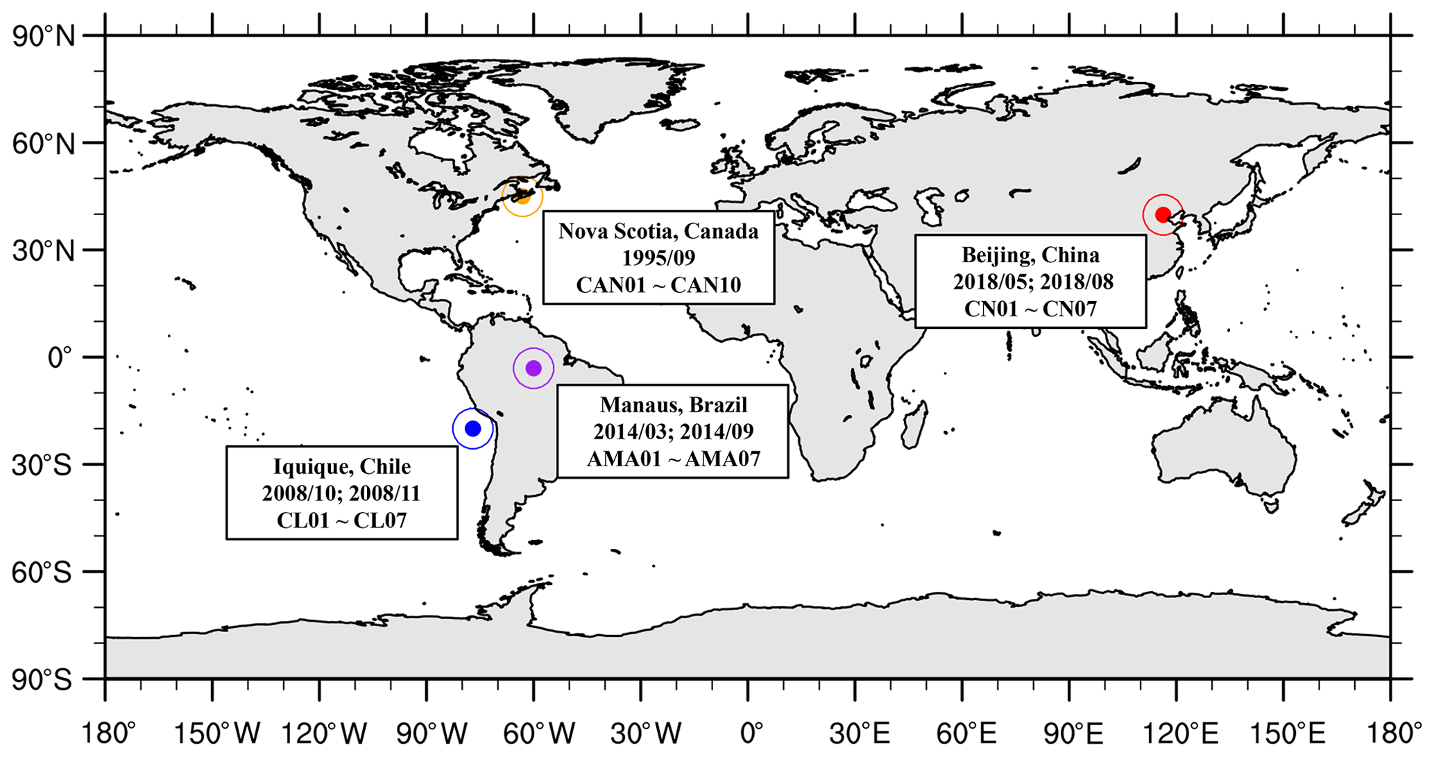
Figure 4 The geographical distribution of 31 selected cloud cases in the four aircraft campaigns. The text boxes provide the locations, the periods, and the names of the cloud cases for each campaign.

Table 2 An overview of the four aircraft campaigns in this study.

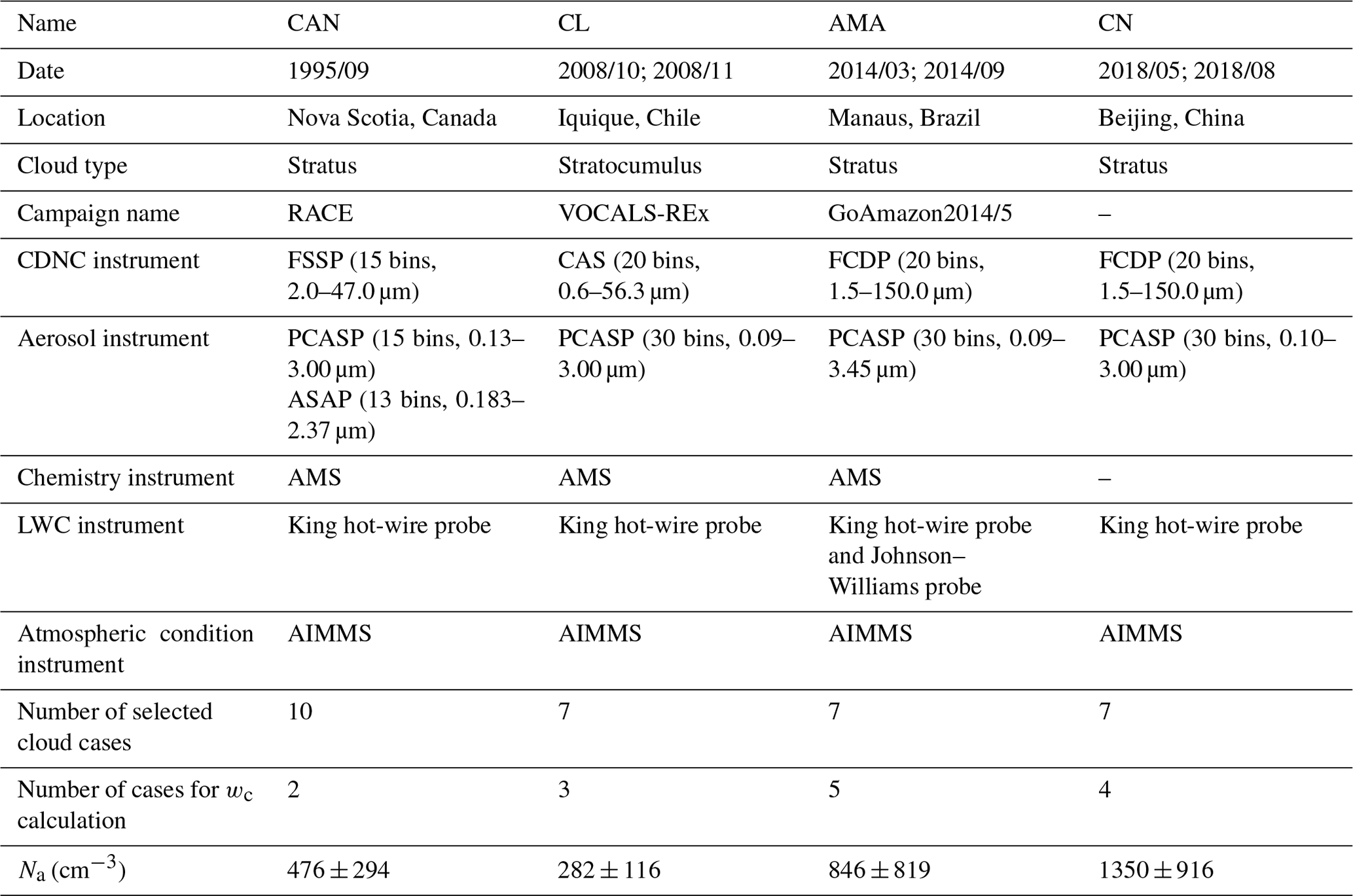
Note: N_a (cm⁻³) is the integrated number of particles detected by aerosol instruments and averaged within 100 m below the cloud base. The definition of cloud base and selection of cloud cases refer to Sect. 3.2.1. Calculation of w_c refers to Sect. 3.2.3.

Aerosol- and cloud-measuring instruments utilized in the four campaigns are briefly presented in Table 2. The observed variables mainly include the CDNC, the cloud liquid water content (LWC), the aerosol number-size distribution, the chemical compositions of aerosol, and atmospheric condition parameters. For the measurement of the CDNC, the forward scattering spectrometer probe (FSSP) was used in the CAN campaign. The cloud, aerosol, and precipitation spectrometer (CAS) was used in the CL campaign. The fast cloud droplet probe (FCDP) was used in the AMA and CN campaigns. Although FCDP, FSSP, or CAS can observe cloud droplets with a particle size up to 150 µm, we only integrated the number for droplets with a particle size of 2 to 30 µm to derive the CDNC. Because cloud droplets larger than 30 µm are subject to collision–coalescence, and droplets smaller than 2 µm may be deactivated by evaporation (Fountoukis and Nenes, 2005). For the measurements of the LWC, the King hot-wire probe was used in all campaigns, and the Johnson–Williams probe was also equipped as an alternative option in GoAmazon2014/5. In terms of the aerosol observation, all the four campaigns utilized an onboard passive cavity aerosol spectrometer probe (PCASP), and some flights during the CAN campaign used the atmospheric solids analysis probe (ASAP), providing aerosol number concentration in multiple size bins roughly from 0.1 to 3 µm. We integrated the number for particles within the detected size range to determine N_a. In the CAN, AMA, and CL campaigns, the mass concentrations of aerosol chemical species, including NH${}_{\mathrm{4}}^{+}$, NO${}_{\mathrm{3}}^{-}$, SO${}_{\mathrm{4}}^{\mathrm{2}-}$, Cl⁻, and organic aerosol (OA), were measured using the aerodyne aerosol mass spectrometer (AMS). The CN campaign lacked data for aerosol chemical composition (see Sect. 3.2.2). For the CL campaign, five aircraft (i.e., Lockhead C-130, BAe-146, Gulfstream-1, Dornier-228, and Twin Otter) carried out observations (Wood et al., 2011). In order to ensure data integrity and consistency for aerosol number-size distribution and chemical composition measurements in the subsequent analysis, we only selected data from the Gulfstream-1 flights. The atmospheric condition parameters (T, pressure (P), relative humidity (RH), vertical velocity (w)) were mainly observed by the airborne integrated meteorological measurement system (AIMMS), in all campaigns. For the CL campaign, vertical velocity data were not available from the Gulfstream-1 flights; thus, we used the observed w data from the Twin Otter flights that occurred simultaneously with Gulfstream-1 flights. Some meteorological variables that are required by the QDGE scheme, particularly including r_v, r_t, and h, were not available from the aircraft observations. Therefore, we calculated these based on other variables (Sect. 3.2.4). Detailed descriptions of the aforementioned observational instruments and data quality control procedures can be obtained from the relevant publications for the different aircraft campaigns (Li et al., 1998; Peng et al., 2002; Wood et al., 2011; Kleinman et al., 2012; Martin et al., 2016, 2017; Wang et al., 2020).

3.2 Data processing for closure experiment

3.2.1 Data extraction

The flow chart of data extraction and processing is shown in Fig. 5. In the first step, we conducted a screening of observational data to obtain suitable cloud cases fulfilling the following conditions (step 1 in Fig. 5). First, we selected cloud cases with continuous LWC profile with T>0^∘ and LWC ≥0.05 g cm⁻³ in each layer, identifying the height of the cloud base as H_low (see Fig. B1). Second, we checked whether the LWC near the cloud base approximately satisfies the wet adiabatic assumption, that is, nearly free from entrainment. As shown in Fig. B1, we plotted the observed LWC and the adiabatic LWC (LWC_ad) profiles, the later ones were calculated by assuming that LWC increases linearly with the height above cloud base (H_c), i.e., LWC_ad=C_wH_c. C_w is the adiabatic liquid water lapse rate, which is a function of temperature (Brenguier, 1991). For liquid clouds, the value of C_w varies from $\mathrm{0.5}\times {\mathrm{10}}^{-\mathrm{3}}$ to $\mathrm{3.0}\times {\mathrm{10}}^{-\mathrm{3}}$ g m⁻⁴ (Peng et al., 2002). For the cases shown in Fig. B1, C_w ranges from $\mathrm{0.6}\times {\mathrm{10}}^{-\mathrm{3}}$ to $\mathrm{2.8}\times {\mathrm{10}}^{-\mathrm{3}}$ g m⁻⁴. The mean of C_w in each cloud case is shown in Table B2. Considering that the entrainment rate e was set to $\mathrm{1.0}\times {\mathrm{10}}^{-\mathrm{3}}$ m⁻¹ (weak entrainment, Barahona and Nenes, 2007) when running the QDGE scheme to be close to the real atmosphere, we identify the nearly adiabatic part in the cloud case (i.e., data sampled between H_low and H_high in Fig. B1) for obtaining the observed cloud properties for evaluating the simulation. Third, we exclude the impact of collision–coalescence in the selected cloud cases, by ensuring that the water contents of cloud droplets with size greater than 30 µm were less than 0.05 g cm⁻³. Finally, we checked to make sure each cloud case has N_a larger than CDNC. Ultimately, 31 eligible cloud cases were selected, as shown in Fig. B1. Table B2 listed the observed data in the selected cloud cases, CDNC_O and LWC were averaged over the adiabatic part of each cloud case, and N_a and RH were averaged within 100 m below the cloud base.

As shown in step 2 of Fig. 5, we classified data samples of each cloud case into cloudy and clear conditions by utilizing the following criteria. Data samples inside the cloud (cloudy condition) require that LWC ≥0.05 g cm⁻³, CDNC >10 g cm⁻³, and RH ≥99.5 %, and data samples outside the cloud (clear condition) require that LWC <0.05 g cm⁻³, N_a>10 cm⁻³, and RH <99.5 %.

During each flight, the sampling along the horizontal flight track was continuous, which allowed us to better characterize the cloudy conditions or atmospheric conditions inside or outside the cloud. In all 31 selected cloud cases, we were able to extract data samples at nl levels (l_d, $d=\mathrm{1},\mathrm{2}$, …, nl from the cloud base, where nl is usually 4 and at least 2) along horizontal flight tracks in each cloud case and calculated the mean value of the observed variable v ($V_{v,l_{\mathrm{d}}}$) along the horizontal track in each level l_d. $V_{v,l_{\mathrm{d}}}$ is then extended to the vertical model levels (L_f, f=1, 2, …, NL, where L_f refers to the interfaces of the vertical layers in the model, i.e., $\mathrm{\Delta }z=L_{f+\mathrm{1}}-L_f$) for running the QDGE scheme, which is step 3, as shown in Fig. 5. The extension proceeded with the following rules: the meteorological variable profiles in clear conditions, such as T, P, and r_t, were extended downwards to the surface by using hydrostatic equation and ideal gas law, then extended to the top by linear extrapolation, and interpolated between l₁ and l_nl. The aerosol mass and number profiles were extended to surface and top by linear extrapolation and interpolated between l₁ and l_nl. RH was filled between l₁ and l_nl by linear interpolation.

For each cloud case, the data samples in the clear air were used to obtain aerosol-related input information for the model simulations (number and mass concentrations of aerosol components in different particle size sections) and the profiles of meteorological parameters. The data samples in cloudy conditions were used to obtain the vertical velocity and LWC as input for the model and to provide measured CDNC for comparisons with model results and closure verification. Here, LWC of the host model was converted into q_w to calculate the initial r_t and h in the QDGE scheme (Fig. 2 and Eqs. 8–12). These are steps 4, 5, and 6, as shown in Fig. 5 and described in the next three subsections.

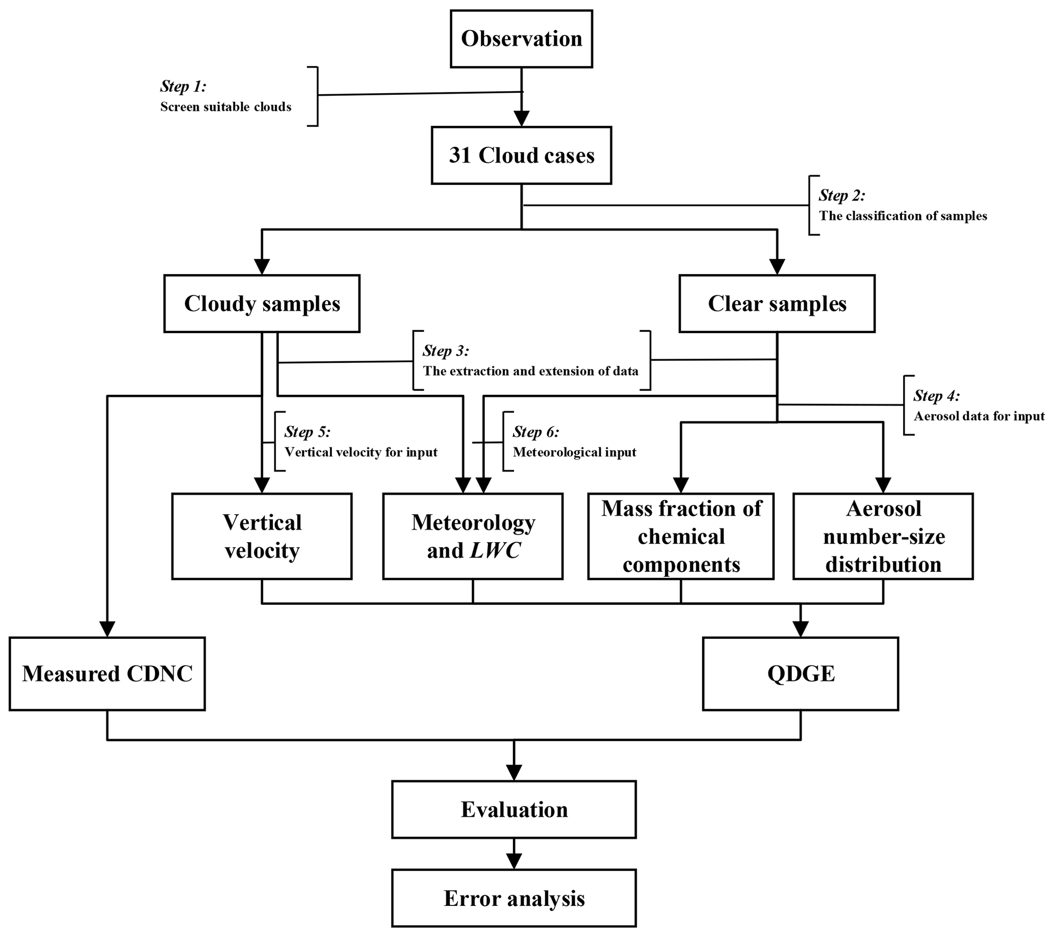
Figure 5 A flow chart to schematically show the data extraction and processing for this work.

3.2.2 Aerosol data for input

In each of the cloud cases from the different aircraft campaigns, aerosol number concentrations N_{a_j} ($j=\mathrm{1},\mathrm{\dots },nj$, where nj is the number of size bins detected in observation; see Table 2) sampled by ASAP or PCASP were categorized in 13, 15, or 30 bins. The size-resolved aerosol number concentrations were subsequently interpolated to a common particle size distribution (PSD) with six prescribed size sections for model input based on the following method (as depicted in Fig. 6). First, we used the aerosol number concentration in each size bin of the PCASP (or ASAP) data to fit a continuous PSD using cubic spline interpolation (Fig. 6b). Second, we integrated the fitted PSD to obtain the aerosol number concentration N_{a_k} (k=1, …, 6) in the aerosol size sections employed by the QDGE scheme (the dry aerosol particle radius boundaries are at 0.050, 0.088, 0.155, 0.274, 0.483, 0.851, 1.500 µm, as shown in Fig. 6c). By utilizing this method, the total N_a obtained by integration over the six QDGE sections was slightly different from the observed total aerosol number due to the fitting of PSD; thus, we further weighed the total fitted aerosol number concentration by the observed aerosol number to ensure the conservation of total number concentration (i.e., the total N_a integrated over the QDGE sections in Fig. 6c is the same as the aerosol number integrated over the observed PSD in Fig. 6a). Finally, the PSD of the aerosol number concentration in six sections (Fig. 6c) was used as input to the QDGE scheme.

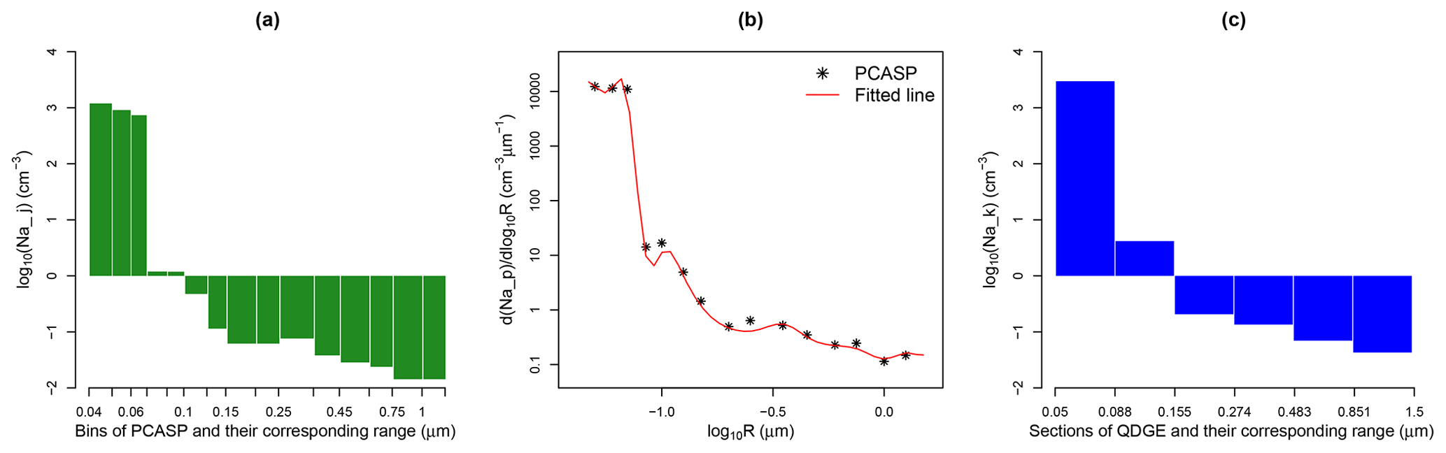
Figure 6 The processing of the observed aerosol number-size distribution for the input to the QDGE scheme: (a) the observed aerosol number concentration in each size bin sampled by PCASP, (b) the particle size distribution curve (red line) fitted to the observations (the asterisks refer to the observations that were derived from panel a), and (c) aerosol number concentration in six size sections, as prescribed in model simulations with the QDGE scheme.

For each of the CAN, AMA, and CL campaigns, the AMS provided measurements of chemical components over the entire campaign, providing concentrations of NH${}_{\mathrm{4}}^{+}$, NO${}_{\mathrm{3}}^{-}$, SO${}_{\mathrm{4}}^{\mathrm{2}-}$, Cl⁻, and OA. The various chemical components in the aerosol were assumed to be internally mixed; thus, all aerosol particles with the same size have the same composition. To obtain the PSD of mass concentration of each chemical component, we made use of the AMS measurements. For continental campaigns such as CN and AMA, we assumed that aerosols are composed of NH₄NO₃, (NH₄)₂SO₄, NH₄Cl, and OA (Shilling et al., 2018; Zhou et al., 2019; Li et al., 2020). For coastal or oceanic campaigns such as CAN and CL, we took sea salt (NaCl) into account, too. For the CAN, AMA, and CL campaigns, we converted the AMS data of ion mass (AMS_ci, ci is NO${}_{\mathrm{3}}^{-}$, SO${}_{\mathrm{4}}^{\mathrm{2}-}$, Cl⁻, or OA) to the mass of each chemical component (m_c, c is NH₄NO₃, (NH₄)₂SO₄, NH₄Cl, OA, or NaCl).

$$\begin{array}{}\text{(15)}& {\displaystyle }{m}_{{\mathrm{NH}}_{\mathrm{4}}{\mathrm{NO}}_{\mathrm{3}}}={\displaystyle \frac{{\mathrm{AMS}}_{{\mathrm{NO}}_{\mathrm{3}}^{-}}}{M_{{\mathrm{NO}}_{\mathrm{3}}^{-}}}}{M}_{{\mathrm{NH}}_{\mathrm{4}}{\mathrm{NO}}_{\mathrm{3}}},\text{(16)}& {\displaystyle }{m}_{({\mathrm{NH}}_{\mathrm{4}}{)}_{\mathrm{2}}{\mathrm{SO}}_{\mathrm{4}}}={\displaystyle \frac{{\mathrm{AMS}}_{{\mathrm{SO}}_{\mathrm{4}}^{\mathrm{2}-}}}{M_{{\mathrm{SO}}_{\mathrm{4}}^{\mathrm{2}-}}}}{M}_{({\mathrm{NH}}_{\mathrm{4}}{)}_{\mathrm{2}}{\mathrm{SO}}_{\mathrm{4}}},\text{(17)}& {\displaystyle }{m}_{{\mathrm{NH}}_{\mathrm{4}}\mathrm{Cl}}={\displaystyle \frac{(\mathrm{1}-\mathit{\alpha }){\mathrm{AMS}}_{{\mathrm{Cl}}^{-}}}{M_{{\mathrm{Cl}}^{-}}}}{M}_{{\mathrm{NH}}_{\mathrm{4}}\mathrm{Cl}},\text{(18)}& {\displaystyle }{m}_{\mathrm{NaCl}}={\displaystyle \frac{\mathit{\alpha }{\mathrm{AMS}}_{{\mathrm{Cl}}^{-}}}{M_{{\mathrm{Cl}}^{-}}}}{M}_{\mathrm{NaCl}},\text{(19)}& {\displaystyle }{m}_{\mathrm{OA}}={\mathrm{AMS}}_{\mathrm{OA}},\end{array}$$

where M_ci and M_c are the molecular weights of ion ci and chemical component c, respectively. Here, we assume that concentrations of NH${}_{\mathrm{4}}^{+}$ are sufficiently high to balance all anions. The mass of sea salt in different campaigns is controlled by a given factor α to partition the amount of Cl⁻ in sea salt and continental chemical components. We set the values of α as 0, 90 %, and 95 % for the AMA, CAN, and CL campaigns. That is, 90 % and 95 % of Cl⁻ are attributed to sea salt in the coastal campaign CAN and the oceanic campaign CL, respectively. Based on the calculated mass concentration of each chemical component, the average density of aerosol can be obtained:

$$\begin{array}{}\text{(20)}& {\mathit{\rho }}_{\mathrm{a}}={\displaystyle \frac{{\sum }_{c=\mathrm{1}}^{\mathrm{5}}{m}_c}{{\sum }_{c=\mathrm{1}}^{\mathrm{5}}{m}_c/{\mathit{\rho }}_c}},\end{array}$$

where ρ_c is the density of each component c, and they are 1725, 1769, 1527, 1900, and 1400 kg m⁻³ for NH₄NO₃, (NH₄)₂SO₄, NH₄Cl, NaCl, and OA, respectively (Ferek et al., 1998; Nakao et al., 2013). Consequently, we can obtain the mass concentration (unit kg cm⁻³) of each component c in section k following this equation:

$$\begin{array}{}\text{(21)}& {\mathrm{Mass}}_{c,k}={\displaystyle \frac{m_c}{{\sum }_{c=\mathrm{1}}^{\mathrm{5}}{m}_c}}\cdot N_{\mathrm{a}\mathit{\_}k}{\displaystyle \frac{\mathrm{4}\mathit{\pi }}{\mathrm{3}}}{R}_k^{\mathrm{3}}{\mathit{\rho }}_{\mathrm{a}},\end{array}$$

where R_k is the median radius of section k.

Since no AMS data are available for the CN campaign, we assumed the mass fraction of different chemical components according to contemporaneous measurements in Beijing, China (Zhou et al., 2019; Li et al., 2020), as shown in Table B3. Under the assumption of ρ_a=1600 kg m⁻¹ (Zamora et al., 2019), Mass_c,k in the CN campaign can be obtained from Eq. (21).

Finally, we obtained the number concentration of total aerosol and the mass concentration of each chemical component from PCASP/ASAP and AMS measurements in each cloud case and calculated aerosol number and mass concentrations in six prescribed size sections following the above procedures (step 4 in Fig. 5). We then used the aerosol information as input to drive the QDGE scheme.

3.2.3 Vertical velocity for input

The averaged updraft velocity (w₊) and subgrid vertical velocity (w_sub) obtained from the observed vertical velocity (w) samples in clouds were used to calculate w_c ($w_{\mathrm{c}}=w_{+}+w_{\mathrm{sub}}$) as input for running the QDGE scheme (step 5 in Fig. 5). The updraft velocity is a key variable for parameterizing aerosol activation. Peng et al. (2005) pointed out that using a characteristic value of the vertical velocity distribution (0.8 times the standard deviation of the distribution) is a good approximation for simulating the nucleated cloud droplet number of marine stratus when running the parcel model. Meskhidze et al. (2005) also gave a method to calculate w₊, which had the optimal closure for cumulus and stratocumulus clouds. Here, we derived a universal method for calculating w₊ in stratus and stratocumulus based on the above two studies.

According to Meskhidze et al. (2005), the averaged updraft velocity (w₊) can be calculated by probability density function (PDF) of w, p(w):

$$\begin{array}{}\text{(22)}& w_{+}={\displaystyle \frac{{\int }_{\mathrm{0}}^{\mathrm{\infty }}wp\left(w\right)\mathrm{d}w}{{\int }_{\mathrm{0}}^{\mathrm{\infty }}p\left(w\right)\mathrm{d}w}}.\end{array}$$

For the normal PDF with the mean velocity w₀ and standard deviation σ, p(w) can be represented as

$$\begin{array}{}\text{(23)}& p\left(w\right)={\displaystyle \frac{\mathrm{1}}{\sqrt{\mathrm{2}\mathit{\pi }}\mathit{\sigma }}}\exp \left(-{\displaystyle \frac{(w-w_{\mathrm{0}}{)}^{\mathrm{2}}}{\mathrm{2}{\mathit{\sigma }}^{\mathrm{2}}}}\right)=\mathit{\beta }\mathit{\varphi }\left(\mathit{\omega }\right),\end{array}$$

where $\mathit{\omega }=\mathit{\beta }w+\mathit{\gamma }$, $\mathit{\beta }=\mathrm{1}/\mathit{\sigma }$, $\mathit{\gamma }=-w_{\mathrm{0}}/\mathit{\sigma }$, and ϕ(ω) is the standard normal PDF.

Using Eq. (23) in Eq. (22), we obtain

$$\begin{array}{}\text{(24)}& w_{+}={\displaystyle \frac{\mathit{\varphi }\left(\mathit{\gamma }\right)}{(\mathrm{1}-\mathrm{\Phi }(\mathit{\gamma }\left)\right)\mathit{\beta }}}-{\displaystyle \frac{\mathit{\gamma }}{\mathit{\beta }}}={\displaystyle \frac{\mathit{\varphi }\left(\mathit{\gamma }\right)}{\left(\mathrm{1}-\mathrm{\Phi }\left(\mathit{\gamma }\right)\right)}}\mathit{\sigma }+w_{\mathrm{0}},\end{array}$$

where Φ(γ) is the cumulative distribution function of the standard normal PDF that can be represented by error function (erf):

$$\begin{array}{}\text{(25)}& \mathrm{\Phi }\left(\mathit{\gamma }\right)=\underset{-\mathrm{\infty }}{\overset{\mathit{\gamma }}{\int }}\mathit{\varphi }\left(t\right)\mathrm{d}t={\displaystyle \frac{\mathrm{1}}{\mathrm{2}}}\left(\mathrm{1}+\mathrm{erf}\left({\displaystyle \frac{\mathit{\gamma }}{\sqrt{\mathrm{2}}}}\right)\right).\end{array}$$

Especially, when w₀=0,

$$\begin{array}{}\text{(26)}& w_{+}={\displaystyle \frac{\mathit{\varphi }\left(\mathrm{0}\right)}{(\mathrm{1}-\mathrm{\Phi }(\mathrm{0}\left)\right)}}\mathit{\sigma }=\sqrt{{\displaystyle \frac{\mathrm{2}}{\mathit{\pi }}}}\mathit{\sigma }\cong \mathrm{0.8}\mathit{\sigma },\end{array}$$

which is consistent with the characteristic velocity pointed by Peng et al. (2005) used for assessing cloud droplet closure for stratocumulus clouds sampled in the CAN campaign.

A subgrid vertical velocity (w_sub) is needed for the QDGE scheme, and it can be derived from the square root of the turbulent kinetic energy (TKE) following Morrison and Pinto (2005):

$$\begin{array}{}\text{(27)}& w_{\mathrm{sub}}=\sqrt{{\displaystyle \frac{\mathrm{2}}{\mathrm{3}}}\mathrm{TKE}},\end{array}$$

where the TKE is given by

$$\begin{array}{}\text{(28)}& \mathrm{TKE}={\displaystyle \frac{\mathrm{1}}{\mathrm{2}}}\left(\stackrel{\mathrm{‾}}{(u^{\prime }{)}^{\mathrm{2}}}+\stackrel{\mathrm{‾}}{(v{}^{\prime }{)}^{\mathrm{2}}}+\stackrel{\mathrm{‾}}{(w{}^{\prime }{)}^{\mathrm{2}}}\right),\end{array}$$

In this study, we assume that no horizontal movement occurs in cloud during the horizontal flight tracks, that is, $\stackrel{\mathrm{‾}}{(u{}^{\prime }{)}^{\mathrm{2}}}=\stackrel{\mathrm{‾}}{(v{}^{\prime }{)}^{\mathrm{2}}}=\mathrm{0}$ and $\stackrel{\mathrm{‾}}{(w{}^{\prime }{)}^{\mathrm{2}}}={\mathit{\sigma }}^{\mathrm{2}}$. Therefore, the subgrid vertical velocity can be represented by σ:

$$\begin{array}{}\text{(29)}& w_{\mathrm{sub}}={\displaystyle \frac{\mathit{\sigma }}{\sqrt{\mathrm{3}}}}.\end{array}$$

If the observed w in each selected cloud case obeyed the normal distribution, we could calculate w_c ($w_{\mathrm{c}}=w_{+}+w_{\mathrm{sub}}$) following Eqs. (24) and (29) as input for running the QDGE scheme easily. We checked the normality of w distribution by drawing a quantile–quantile (Q–Q) plot using the observed w values along the horizontal flight track of the cloud case, taking CN01 as an example in Fig. 7. The linearity between the Q–Q plot of observed w samples and a standard normal distribution indicates that w data do indeed follow the normal distribution.

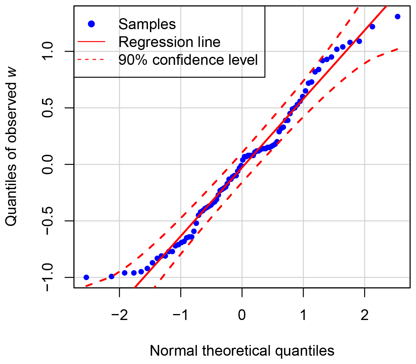
Figure 7 A normal quantile–quantile plot for comparing the observed w sampled by aircraft in cloud case CN01 with a standard normal distribution. The linearity of the data points (blue) suggests that the observed w are normally distributed.

In the four campaigns of this study, four cloud cases in CN, two cases in CAN, five cases in AMA, and three cases in CL have enough data samples to obtain the PDF of w (Table 2), as plotted for checking the normality of w distribution in Fig. B2. However, the w PDF in two of the CAN cloud cases does not conform to the normal distribution very well (panels 5 and 6 in Fig. B2). So, we used the mean and standard deviation of w distribution in Peng et al. (2005) to obtain w_c in the CAN campaign. For the CN, AMA, and CL campaigns, we directly calculated the w_c from available data samples for the cloud cases plotted in Fig. B2 and used their mean values for cloud cases lacking enough w values in each campaign (Table B2).

3.2.4 Meteorological input

Some meteorological variables (T, P, RH, and LWC) can be obtained from AIMMS measurements directly, though others (r_v, r_t, and h) need to be calculated according to available variables (step 6 in Fig. 5). We obtained r_v by the following equation:

$$\begin{array}{}\text{(30)}& r_{\mathrm{v}}={\displaystyle \frac{\mathit{\epsilon }{e}_{\ast }\mathrm{RH}}{P-e_{\ast }\mathrm{RH}}},\end{array}$$

where e_∗ can be estimated by referring to Murray (1967):

$$\begin{array}{}\text{(31)}& e_{\ast }=\mathrm{6.1078}{e}^{\left(\frac{\mathrm{17.2694}(T-\mathrm{273.16})}{T-\mathrm{35.86}}\right)}.\end{array}$$

Then, r_t and h can be obtained by Eqs. (8) and (9) from r_v and other available variables. All meteorological variables were extracted and interpolated to model levels, as described in Sect. 3.2.1. The profiles of measured meteorological variables served as the initial state to drive the QDGE scheme.

3.2.5 Determination of N_sub

As mentioned in Sect. 2.1, the QDGE scheme simulates vertical profiles of supersaturation to determine S_max, for a vertical grid with the size $\mathrm{\Delta }{z}_{\mathrm{s}}=\mathrm{\Delta }z/N_{\mathrm{sub}}$, where Δz is the grid size of the atmospheric host model. The accuracy of the simulated supersaturation profile generally increases with N_sub, though large values of N_sub imply higher computational burdens. For applications of the QDGE scheme in atmospheric models, it is therefore important to determine an optimal value of N_sub that yields sufficiently accurate supersaturation profiles at acceptable costs.

Figure 8a plots the vertical profiles of S simulated by the QDGE scheme with different N_sub values for cloud case CN01. The results show that each profile with N_sub≥3 produces a well-defined maximum of S (S_max), which approaches a stable value as N_sub is further increased. All cases seem to converge to a similar value as S_max with N_sub=150, as plotted in Fig. 8a. Figure 8b shows the variation of S_max with the increasing N_sub for all cloud cases in the four campaigns. Overall, S_max fluctuates dramatically with N_sub<10, but plateaus when N_sub is greater than 60 (10 for CAN). Results obtained for N_sub=150 and N_sub=60 are similar. The mean relative error and correlation coefficient between S_max with N_sub=150 and that with N_sub=60 are 1.97 % and 0.9997, respectively. Therefore, we used N_sub=60 in this study (N_sub=10 for CAN). Further discussion regarding the selection of N_sub is provided in Sect. 5.

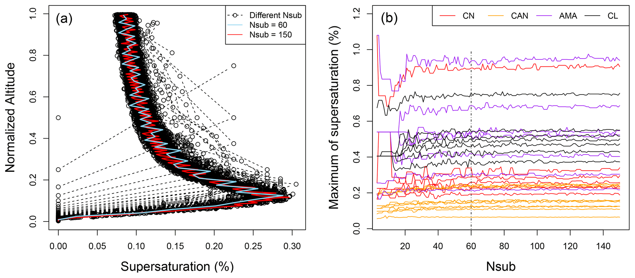
Figure 8 (a) Vertical profiles of the simulated supersaturation for different N_sub (1–150) in the QDGE scheme for cloud case CN01. (b) Changes of the maximum supersaturation with different N_sub for all cloud cases in the four campaigns.

3.3 Statistical parameters for evaluation and error analysis

The QDGE scheme simulates the CDNC (CDNC_M) in each cloud case, based on S_max. Noting that CDNC_M is not exactly the same as N_CCN here, as we take wet particles with a size between 2 and 30 µm to compare with the observed one. Considering that aerosol activation is particularly efficient in the vicinity of the cloud base in stratus and convective clouds, the QDGE scheme only calculates the CDNC at the cloud base (Sect. 2.1). Here, we considered the effect of weak entrainment on the vertical profile of the cloud droplet number mixing ratio to be close to the real cloud base in the atmosphere (Sect. 3.2.1). Therefore, we evaluated the performance of the QDGE scheme by comparing CDNC_M with the vertically average value of the observed CDNC (CDNC_O) in the nearly adiabatic part of the cloud (between H_low and H_high in Fig. B1) (Sect. 3.2.1), given by

$$\begin{array}{}\text{(32)}& {\mathrm{CDNC}}_O={\displaystyle \frac{\mathrm{1}}{N_O}}{\sum }_{H=H_{\mathrm{low}}}^{H_{\mathrm{high}}}{\mathrm{CDNC}}_{O,H},\end{array}$$

where N_O is the number of samples between H_low and H_high, and CDNC_O,H is the observed CDNC in height H.

Correspondingly, the mean relative error (MRE) of each cloud case can be calculated, as follows:

$$\begin{array}{}\text{(33)}& \mathrm{MRE}=\left|{\displaystyle \frac{{\mathrm{CDNC}}_M-{\mathrm{CDNC}}_O}{{\mathrm{CDNC}}_O}}\cdot \mathrm{100}\mathit{\%}\right|,\end{array}$$

where MRE of each cloud case will also be used for subsequent error analysis.

To evaluate the overall accuracy of the QDGE scheme, we also calculated the mean values of CDNC_O, CDNC_M, MRE for cloud cases in each campaign, namely $\stackrel{\mathrm{‾}}{{\mathrm{CDNC}}_O}$, $\stackrel{\mathrm{‾}}{{\mathrm{CDNC}}_M}$, and $\stackrel{\mathrm{‾}}{\mathrm{MRE}}$. Besides, the R² (R is the Pearson correlation coefficient) between the CDNC_O and CDNC_M in each campaign was also calculated.

To quantify the contributions of different physical variables to errors in the simulated CDNC with the QDGE scheme, we calculated the maximum information coefficient (MIC) (Reshef et al., 2011), which provides a measure for the strength of the relationship between each input variable and MRE. MIC can be a good measure to capture the association between the attributive variable and MRE for different types of relationships, such as linear, exponential, and many complex functional relationships (Reshef et al., 2011). There is no need to standardize the data before the MIC calculation, and the calculations have low computational complexity and high robustness. However, it should be noted that the association here does not refer to a specific correlation, such as temporal or spatial correlation, or positive or negative correlation, but refers to the strength of a certain relationship between the variable and MRE. The MIC value is always between 0 and 1. The higher the MIC value, the stronger the association between the input variable and MRE; that is, the input variable contributes more significantly to the MRE. Here, we calculated the MIC base on the minepy package in Python (Albanese et al., 2018), and set the parameters required in MIC as the default settings suggested by the code developers. Different parameters had an insignificant effect on the relative importance of variables and MRE.

We calculated the MIC between MRE and each one of the following input variables: the relative humidity (RH), the mean vertical velocity (w₊), and the subgrid vertical velocity (w_sub) to represent environmental and dynamic conditions; the total aerosol number (N_a) as a proxy of pollution level, the hygroscopicity of aerosol (K_m) weighted by composition volume fraction, and the effective radius of aerosol PSD (R_e,a) to represent the chemical and size properties of the aerosol. Here, K_m and R_e,a are defined as

$$\begin{array}{}\text{(34)}& {\displaystyle }{K}_m={\displaystyle \frac{{\sum }_{c=\mathrm{1}}^{\mathrm{5}}\frac{m_c}{{\mathit{\rho }}_c}{\mathit{\kappa }}_c}{{\sum }_{c=\mathrm{1}}^{\mathrm{5}}\frac{m_c}{{\mathit{\rho }}_c}}},\text{(35)}& {\displaystyle }{R}_{\mathrm{e},\mathrm{a}}={\displaystyle \frac{{\sum }_{j=\mathrm{1}}^{nj}{R}_j^{\mathrm{3}}{N}_{a\mathit{\_}j}}{{\sum }_{j=\mathrm{1}}^{nj}{R}_j^{\mathrm{2}}{N}_{a\mathit{\_}j}}},\end{array}$$

where κ_c, the hygroscopicity of component c, is accounted for variations with relative humidity in the QDGE scheme (Appendix A). R_j represents the middle radius in the jth particle size bin observed by PCASP or ASAP (see Sect. 3.2.2 and Table 2). For MIC calculation, the values of input variables derived from observations are listed in Table B2 for each cloud case.

4 Results

4.1 Closure experiment

The results of the closure experiment are shown in Fig. 9. Almost all CDNC_M values fall within 30 % of the mean observations in the clouds. R² is above 0.94 for all campaigns, which indicates a good agreement between simulation and observation. For the four campaigns covering marine to continental conditions, the $\stackrel{\mathrm{‾}}{\mathrm{MRE}}$ values are all below 26 %. The AMA campaign produces the best agreement between model results and observations, with a $\stackrel{\mathrm{‾}}{\mathrm{MRE}}$ value of 17.30 %. On the other hand, the CN campaign produces a poor agreement, with a $\stackrel{\mathrm{‾}}{\mathrm{MRE}}$ value of 25.90 %. However, cloud droplet number concentrations are underestimated for all cloud cases for the CL campaign (Fig. 9c), which may be related to the high activation ratio (AR, the ratio of N_a to CDNC_O; see Table B2) in this region. AR in all CL cases are higher than 60 %, suggesting that the marine environment is favorable for more aerosol particles to be activated. If particles with a smaller size than the detection limit of PCASP (about 10 nm) are activated, it could lead to an underestimation of the simulated CDNC in the CL campaign.

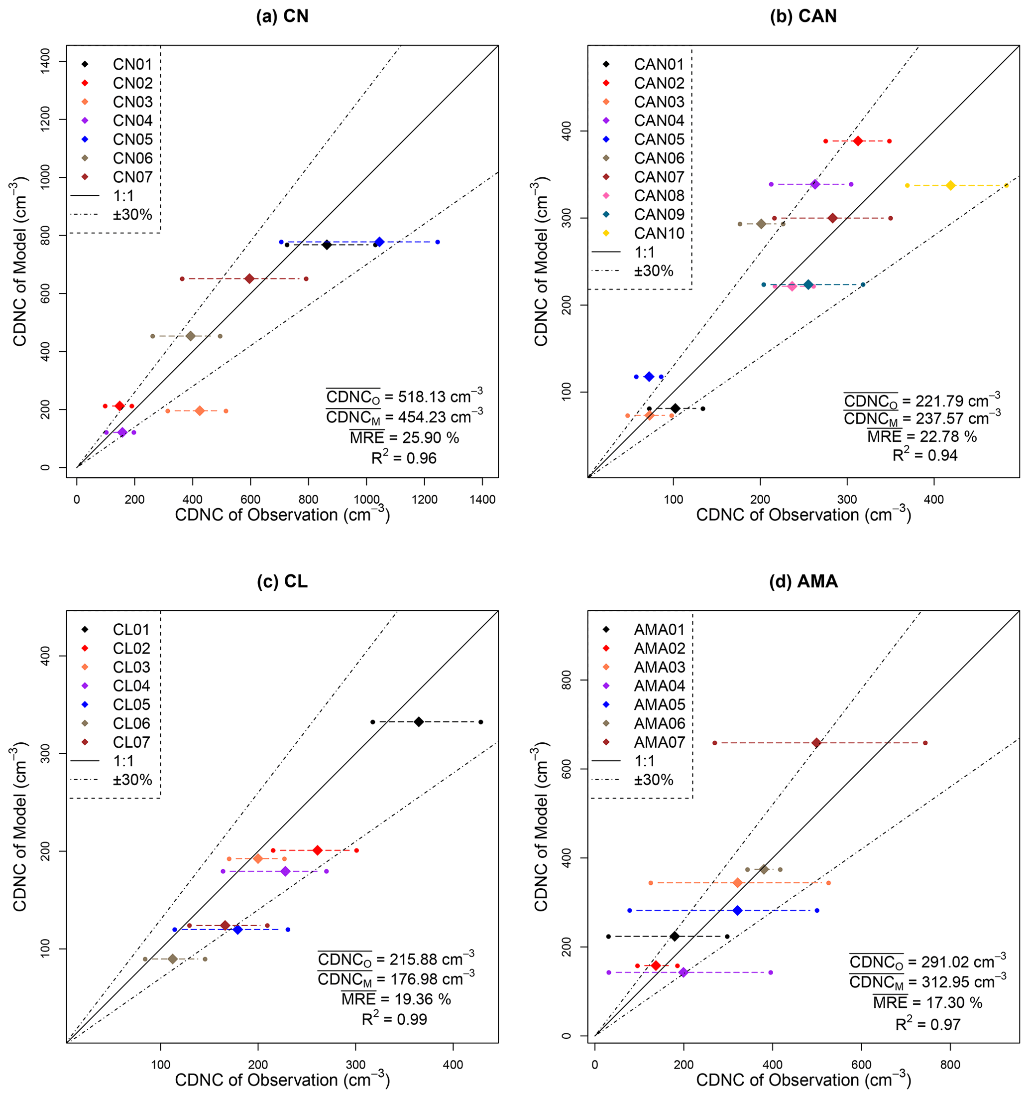
Figure 9 A closure experiment between CDNC_O and CDNC_M for each cloud case in the (a) CN, (b) CAN, (c) CL, and (d) AMA campaigns. The horizontal dashed lines represent the range of the observed CDNC within the 25 % and 75 % quantiles.

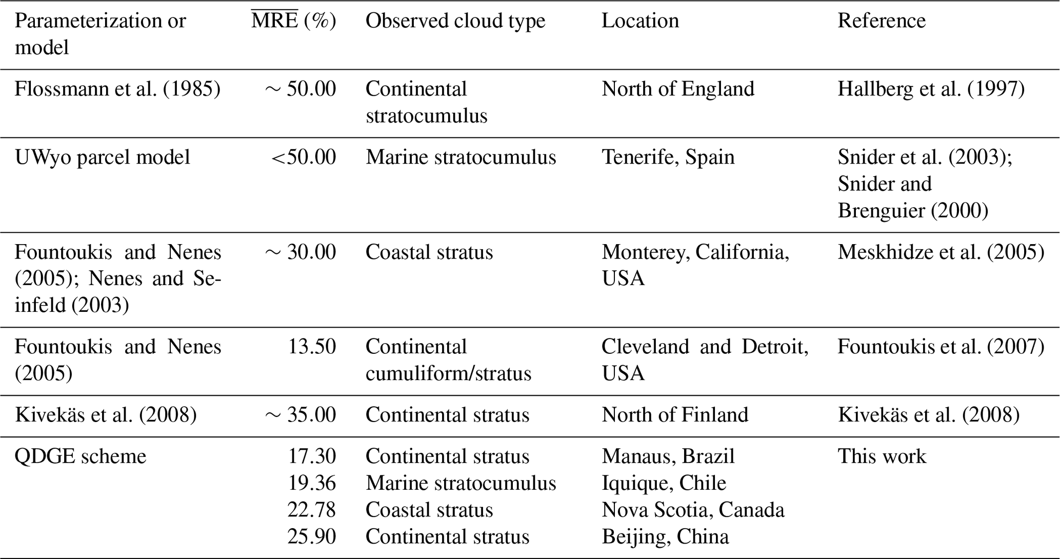
In order to provide further context, we compare the $\stackrel{\mathrm{‾}}{\mathrm{MRE}}$ values of this study to previous studies with different aerosol activation parameterizations and aircraft measurements, as shown in Table 3. The $\stackrel{\mathrm{‾}}{\mathrm{MRE}}$ values are relatively high for those early parameterizations, basically around 50 %. In the two recent decades, the performance of physically based parameterization has been significantly improved, as is evident from a reduction of the $\stackrel{\mathrm{‾}}{\mathrm{MRE}}$ to about 30 %. For instance, one of the schemes (Fountoukis and Nenes, 2005) achieved remarkable closure (with $\stackrel{\mathrm{‾}}{\mathrm{MRE}}$ of 13.5 %) for continental cumuliform/stratus. In this study, the QDGE scheme performs decently (the $\stackrel{\mathrm{‾}}{\mathrm{MRE}}$ values are all below 26 %) in four different regions, indicating that the scheme is suitable for simulations of cloud droplet number concentrations over a wide range of different meteorological conditions and different levels of aerosol pollution.

Table 3 Comparison of results from simulations with previous activation schemes (mainly referring to Fountoukis et al., 2007) and the QDGE method.

4.2 Error analysis

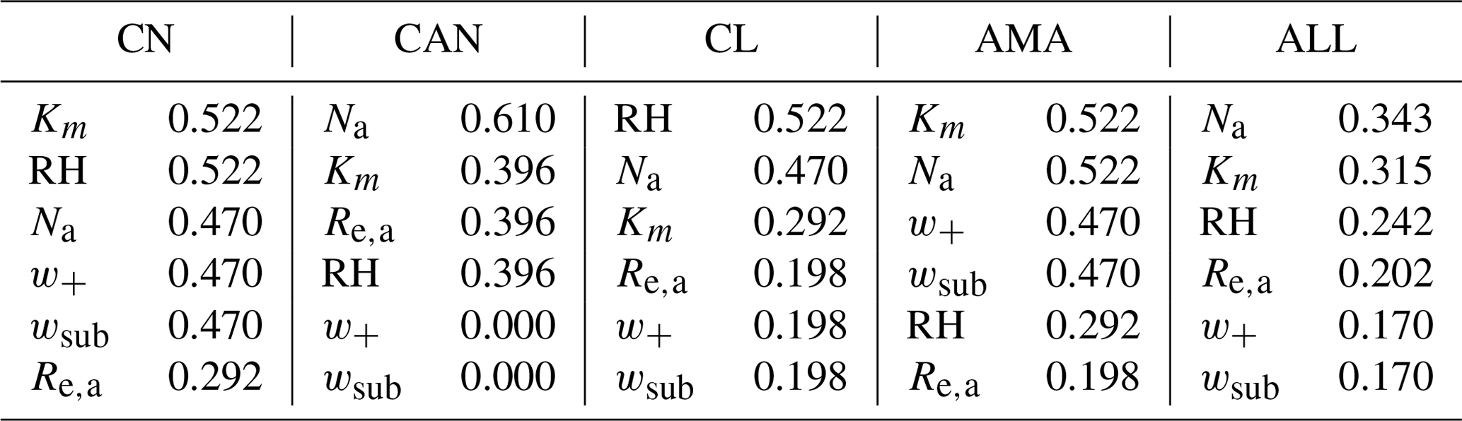
Although the performance of the QDGE scheme is good in different aircraft campaigns, it is useful to analyze sources of biases in the simulations. Following the procedures described in Sect. 3.3, we calculated the MIC between MRE and the input variables of the QDGE scheme, including aerosol properties (K_m and R_e,a), thermodynamic state (RH), pollution level (N_a), and atmosphere dynamic conditions (w₊ and w_sub), as shown in Table B2. The MIC values for all cloud cases and each campaign have been shown in Table 4.

For almost all campaigns, the aerosol number concentration and the hygroscopicity have the most significant impacts on MRE. This is consistent with the change of environmental supersaturation (Eq. 3), according to which the variation of supersaturation S with height is essentially determined by the competition between the production of S by adiabatic cooling and the reduction in S from condensational growth of the particles, the latter mainly depends on the number and solubility of the aerosol particles. In detail, N_a has a greater impact on MRE in marine regions (CAN and CL), but K_m is more significant in continental regions (CN and AMA). In marine regions, where N_a is relatively low (Table 2), a small fluctuation in N_a can cause noticeable changes in the simulated S_max and CDNC, which makes MRE more sensitive to N_a. However, in continental areas, N_a is relatively high, and the change in hygroscopicity becomes more important to MRE. The atmospheric humidity and the dry size of the aerosol particle also have non-negligible impacts on MRE. Both affect the hygroscopic growth of aerosol particles and the reduction in S. Overall, the atmosphere dynamic conditions have the most insignificant impact on MRE, which may be attributed to the weak variation of them in stratus and stratocumulus clouds (Table B2).

The MIC values also help to explain the relatively poor simulation performance of some campaigns. The chemical properties of the aerosol, which affect K_m, are very important for the simulation in the continental region, but the CN campaign lacks AMS data, and we applied the same chemical composition for all cloud cases, based on earlier measurements in this region (Sect. 3.2.2). Given the importance of the chemical properties, simultaneous measurements of chemical components probably would have helped to enhance the accuracy of simulated CDNC for the CN campaign. Another possible cause of biases in simulated CDNC for the CN campaign is a much larger standard deviation of observed N_a (see Table 2) than that of other campaigns, which could be responsible for the error in the simulated CDNC. However, it should be noted that although the CAN campaign is characterized by the presence of coastal clouds and smaller variations in N_a, its MRE is higher than the AMA campaign, which may be related to the application of uniform updraft velocity in simulations for the CAN campaign (Sect. 3.2.3 and Table B2).

Overall speaking, the errors in the simulated CDNC are largely relevant to the missing data in observations (such as CN and CAM campaign); the analysis of MIC and error sources here could provide a good reason to develop and improve measurement strategies in the future aircraft campaigns.

Table 4 The calculated MIC values between MRE and different input variables for each campaign and all cloud cases.

5 Conclusions and discussion

In this paper, we introduce a numerically efficient aerosol activation scheme, which calculates the maximum cloud supersaturation and cloud droplet number concentration (CDNC) by employing a quasi-steady-state approximation of the cloud droplet growth equation (QDGE) scheme. The QDGE scheme utilizes the look-up table and iterative calculation for solving the sublevel variation of supersaturation and deriving the maximum supersaturation and the activated particle number-size distribution in the large-scale grid of climate models. The comparison between the results of the QDGE scheme and a parcel model shows that biases in the maximum supersaturation under different environmental and aerosol conditions are within 0.18 % (with an average of 0.05 %), consistent with the high accuracy of the QDGE scheme. Whereafter, we evaluated the simulated CDNC with worldwide cloud data sampled during four aircraft campaigns, covering a wide range of different meteorological conditions and different levels of aerosol pollution. The aerosol information, updraft velocity, and meteorological conditions were carefully extracted from aircraft measurements and applied to drive the QDGE scheme. The simulated CDNC is compared with the observed correspondence in the nearly adiabatic part of the cloud, for evaluating the performance of the scheme. The average values of the mean relative error in the four campaigns are all within 26 %, indicating that the QDGE scheme can reasonably simulate the activated CDNC on a regional or global scale. We also investigated the potential sources of error in the simulated CDNC and found that the magnitude of the mean relative error is mostly relevant to the aerosol number concentration in marine regions and to aerosol hygroscopicity in continental regions than to other variables in the simulation.

Several points are worthy of mentioning for future work. The QDGE scheme can be further optimized in several aspects. First, N_sub=60 generates reasonably good results in four different regions in this study, but this number is a little high and the computation will be too demanding to apply in general circulation models. Second, the iterative calculation to derive supersaturation in each subgrid level can be computationally expensive. Therefore, both adjustments on N_sub number and optimization on the iteration would be necessary before the QDGE scheme is applied in the climate model. These works would be considered in future studies.

Appendix A: Parameters

The parameters A, B, C, D, and E in Eqs. (1)–(3) are given by

$$\begin{array}{}\text{(A1)}& {\displaystyle }A={\displaystyle \frac{\mathrm{2}{M}_{\mathrm{w}}\mathit{\sigma }}{RT{\mathit{\rho }}_{\mathrm{w}}}},\text{(A2)}& {\displaystyle }B=\mathit{\kappa }{R}_{\mathrm{p}}^{\mathrm{3}},\text{(A3)}& {\displaystyle }C={\displaystyle \frac{{\mathit{\rho }}_{\mathrm{w}}RT}{e_{\ast }{D}_{\mathrm{v}}{}^{\prime }{M}_{\mathrm{w}}}}+{\displaystyle \frac{L_{\mathrm{v}}{\mathit{\rho }}_{\mathrm{w}}}{K_{\mathrm{a}}{}^{\prime }T}}\left({\displaystyle \frac{L_{\mathrm{v}}{M}_{\mathrm{w}}}{RT}}-\mathrm{1}\right),\text{(A4)}& {\displaystyle }D={\displaystyle \frac{g{M}_{\mathrm{w}}{L}_{\mathrm{v}}}{c_{\mathrm{p}}R{T}^{\mathrm{2}}}}-{\displaystyle \frac{g{M}_{\mathrm{a}}}{RT}},\text{(A5)}& {\displaystyle }E={\displaystyle \frac{P{M}_{\mathrm{a}}}{e_{\ast }{M}_{\mathrm{w}}}}+{\displaystyle \frac{M_{\mathrm{w}}{L}_{\mathrm{v}}^{\mathrm{2}}}{c_{\mathrm{p}}R{T}^{\mathrm{2}}}},\end{array}$$

where κ is the aerosol hygroscopicity, σ is the surface tension of the solution–air interface (which is approximated by the surface tension of water here), ρ_w is the density of water, M_w is the molecular weight of water, R is the universal gas constant, T is the temperature, R_p is the dry aerosol particle radius, e_∗ is the saturation vapor pressure, L_v is the latent heat of vaporization, K_a^′ is the modified thermal conductivity of air accounting for non-continuum effects, D_v^′ is the modified diffusivity of water vapor in air accounting for non-continuum effects (Seinfeld and Pandis, 2016), g is the gravitational constant, M_a is the molecular weight of dry air, P is the atmospheric pressure, and c_p is the heat capacity at a constant pressure of dry air.

Petters and Kreidenweis (2007) proposed a parameter κ for representing the hygroscopicity of aerosol with a variety of chemical compounds and provided tabulated values of κ based on laboratory data and modeling. They found that the aerosol water content (the ratio of wet aerosol volume to the dry aerosol volume) parameterized on κ was generally within the experimental uncertainty but biased at low relative humidity (Kreidenweis et al., 2008; Petters and Kreidenweis, 2007). Kreidenweis et al. (2008) evaluated the calculated aerosol water content based on κ with the Aerosol Inorganic Model (AIM; Wexler and Clegg, 2002), which gives evidence for systematically different results at low aerosol water contents for some compounds. In order to improve biases at low relative humidity, the original method was extended to account for variations in κ with relative humidity in the QDGE scheme. Specifically, piecewise-linear relationships between κ and aerosol water activity for different chemical components were determined based on results from AIM.

Appendix B: Tables and figures

Table B1 Aerosol distribution and property parameters (κ and e are aerosol hygroscopicity and entrainment rate, as mentioned in Appendix A and Sect. 2.1, respectively), referring to Whitby (1978) and Ghan et al. (2011).

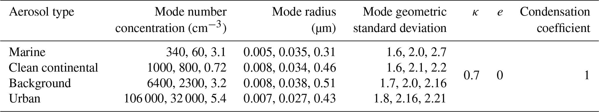
Table B2 A summary of observed (CDNC_O, N_a, RH, and LWC), derived (AR as mentioned in Sect. 4.1, C_w as mentioned in Sect. 3.2.1, K_m and R_e,a as mentioned in Sect. 3.3, and w₊ and w_sub as mentioned in Sect. 3.2.3), simulated, and evaluative (CDNC_M and MRE) variables of each cloud case in four campaigns.

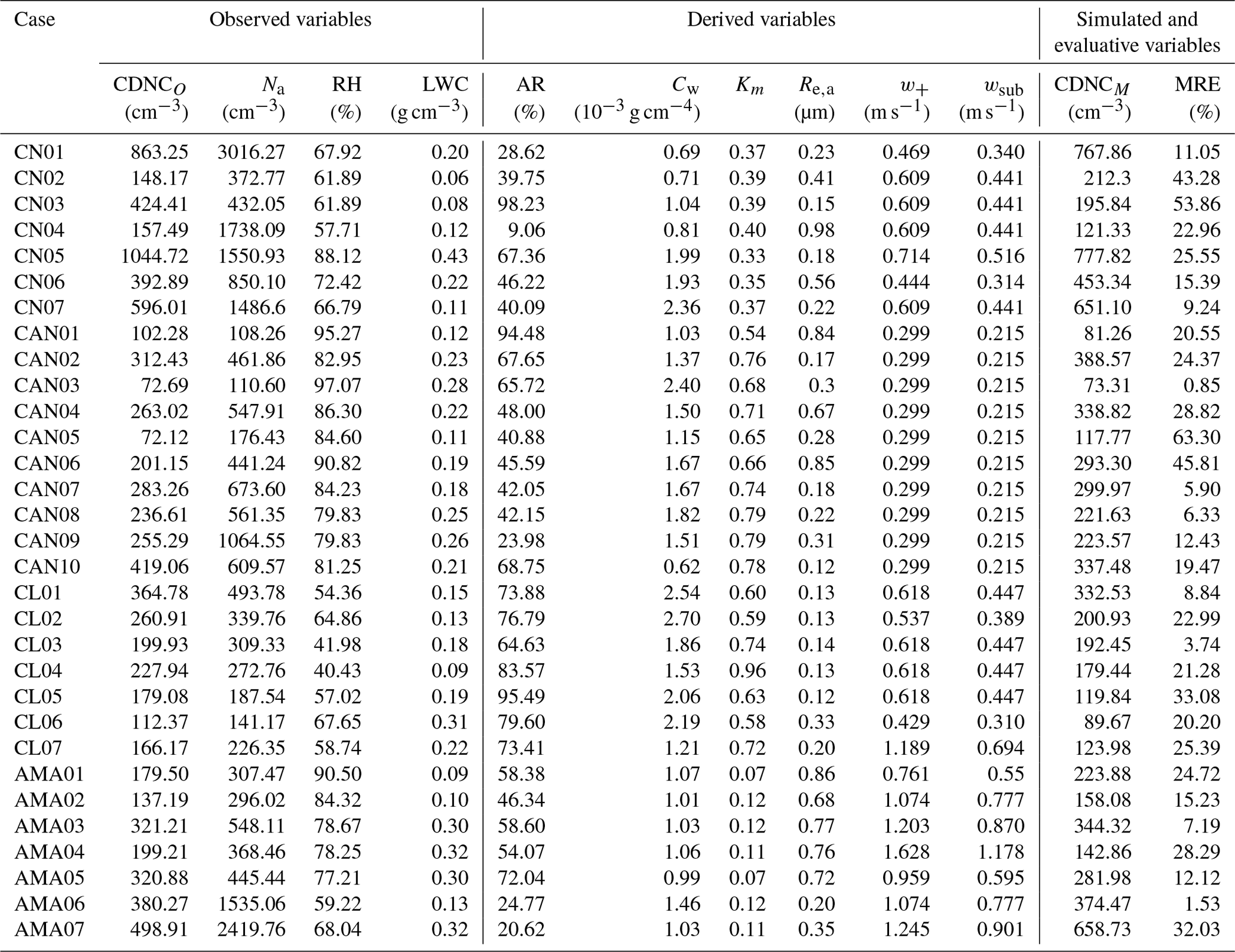
Table B3 The observed mass fractions of different aerosol compositions in Beijing, China, in two previous studies, as well as the assumed fractions used in this work.

^* ACSM: Aerosol Chemical Speciation Monitor.

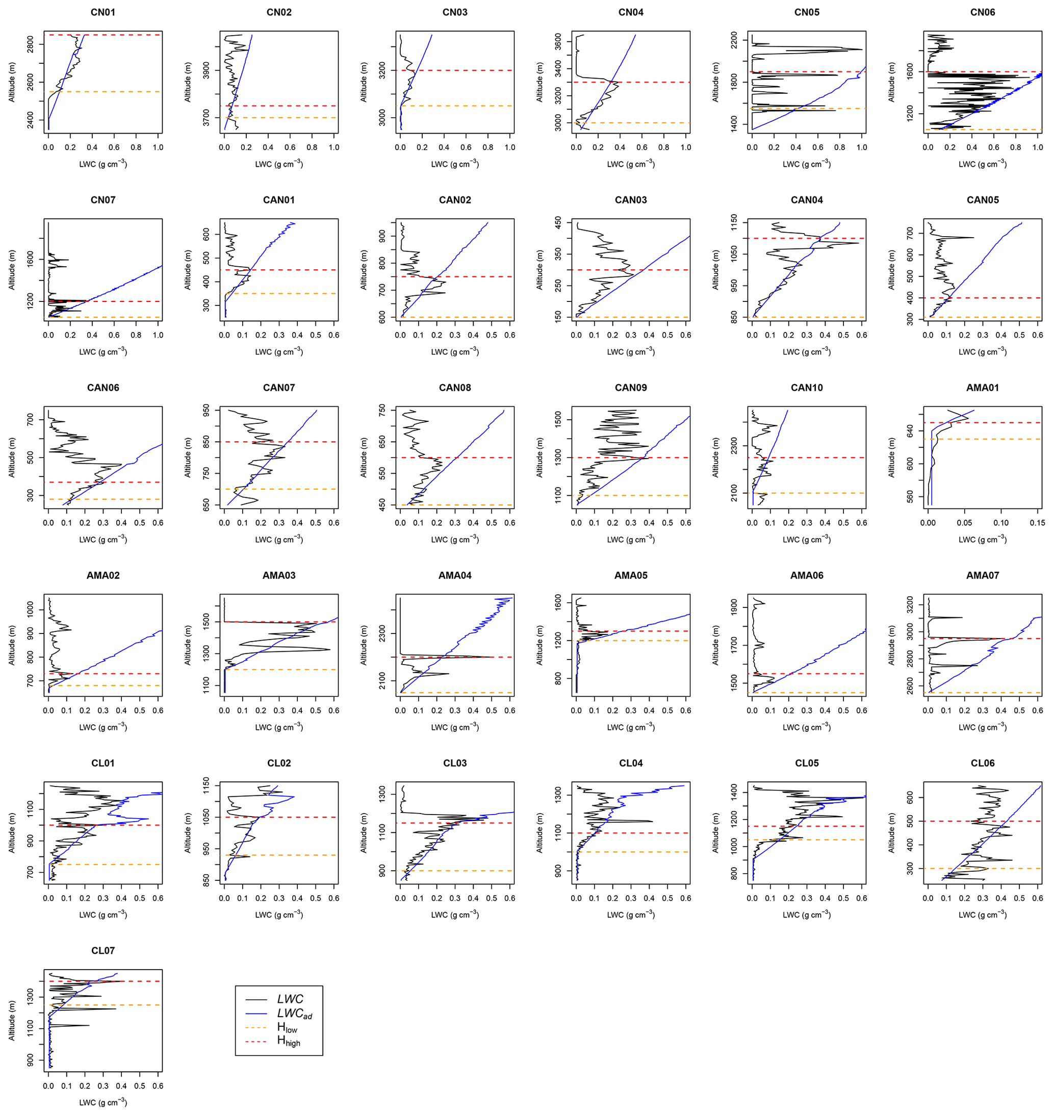
Figure B1 The profiles of observed LWC (black) and adiabatic LWC (LWC_ad, blue) for 31 cloud cases.

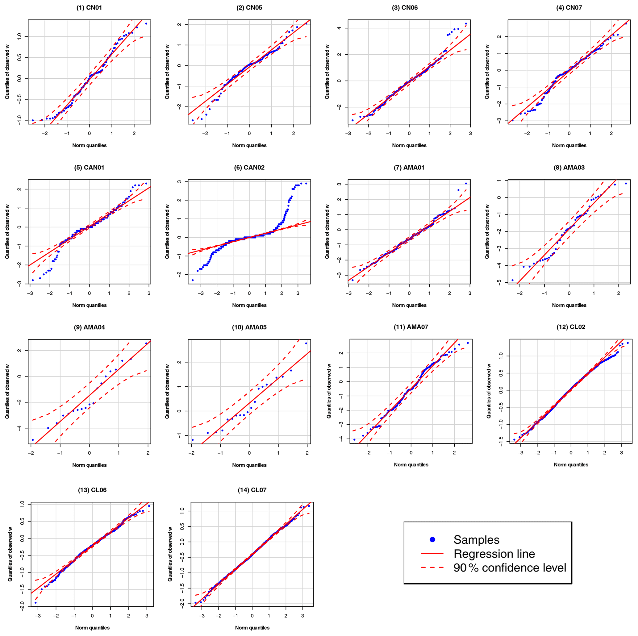
Figure B2 The normal quantile–quantile plot for comparing the observed w sampled by aircraft with a standard normal distribution for each cloud case with sufficient data. The linearity of the data points (blue dots) suggests that the observed w values are normally distributed under a 90 % confidence level.